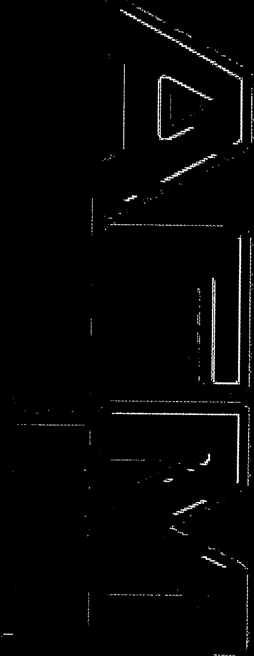
TT-AFM. v 2.2. Users Guide 1 ~ ~ I I I I I I I I I I

Transcription

1 TT-AFM Users Guide v ~ ~

2 Definitions and Symbols The following terms and symbols are used in this document and also appear on the product where safety-related issues occur. General Warning or Caution The exclamation symbol may appear in warning and caution tables in this document. This symbol designates an area where personal injury or damage to the equipment is possible. European Union CE Mark CE The presence of the CE Mark on AFMWorkshop equipment means that it has been designed, tested and certified as complying with all applicable European Union (CE) regulations and recommendations. Warnings/Cautions/Notes The following are definitions of the warnings, cautions and notes that may be used in this manual to call attention to important information regarding personal safety, safety and preservation of the equipment, or important tips. WARNNG Situation has the potential to cause bodily harm or death. CAUTON Situation has the potential to cause damage to property or equipment. NOTE Additional information the user or operator should consider.

3 1. ntroduction to Atomic Force Microscopy ntroduction to the TT-AFM Computer Stage..., Ebox Video Optical Microscope Measuring mages With the T-AFM Operating the Video Microscope Preparing Samples Exchanging Probes Aligning the Light Lever Force Sensor Optically-Assisted Tip Approach Contact Mode maging Vibrating Mode lmaging Software nstallation Procedure... B 3.2. AFM-View Software Pre-Scan Window Files Modes Laser Align Tune Frequency Manual Z Motor Control Range Check Automated Tip Approach Topo Scan Window mage Window Oscilloscope Window Scan Setup Z Feedback Display Tip Retract Scan :3. System Window Tip Approach Z Parameters XYZ Calibration XY Parameters Other Controls Force Distance Curves Video-View Software Contents

4 5. Troubleshooting Saturation of the Photo-Detector Sample Not Mounted Correctly Probe Not Seated Correctly Resonance Saturated False Feedback Scanner at End of Z Range Defective Probe High Resolution lmaging Appendix A: Setting Up the TT-AFM A.1. Selecting a Location A.2. Setting Up the Optical Microscope A.3. Connecting the TT-AFM to the Cables A.4. System Check A.5. Aligning the Video and TT-AFM Microscopes A.6. First Alignment of the Light Lever A.7. nstalling an XYZ Piezoelectric Scanner A.S. Leveling Sample Holder... : A.9. Grounding the TT-AFM Appendix 8: TT-AFM Files Parameter Files Scanner Files Data Files Appendix C: Calibration Appendix D: Noise Floor Appendix E: Probes Appendix F: Technical nformation F.1. Electronic Block Diagrams F.2. Ebox and Modes Pin Assignments Appendix G: Optimizing GPD Parameters Appendix H: Renaming National nstruments DAQ Device Appendix 1: Analyzing Force/Distance Curves... 65

5 n anafm (atomic force microscope), a probe is scanned over a surface and the motion of the probe is monitored to create a three-dimensional image of the surface. These unique instruments are capable of measuring high-resolution images in both ambient air and liquids, with surface features of only a few nanometers in size. The three-dimensional motion of the sample (or probe) is generated by piezoelectric ceramics. These sensitive ceramics allow motions as small as a fraction of a nanometer. Typically, the sample (or probe) is moved in a raster pattern as the probe glides across the surface. _v_2_.2_ 1_ TT_ _A_FM_ u_s_e_rs_g_u_l_de Mi!.!.ilil The light lever can be made more sensitive by vibrating the cantilever with a small piezoelectric ceramic and modulating the light. When the vibrating probe interacts with the surface, the amplitude of vibration may be monitored and used to control the probe's force on the surface. Modern atomic force microscopes include not only a probe and piezoelectric scanner, but additional hardware for bringing the probe rapidly into the proximity of a surface. A video optical microscope is very helpful for operating an AFM. The video microscope helps with aligning the light lever and probe approach, and for finding features for scanning. For an in-depth description of AFM instrumentation, we recommend the book Atomic Force Microscopy by Peter Eaton and Paul West. This book provides a complete theoretical, as well as practical explanation for the design and application of AFMs. OXil'OR.D ATOMC FORCE M CROSCOPY i'ete:r EATON PAUL WEST With this light lever, forces as small as a pica-newton are possible. With such small forces, very small probes may be used. With micro-machining methods, probes can have diameters of only a few nanometers. A light lever sensor is used for controlling the force of the probe on the surface while the sample is scanned. The light lever reflects a laser beam off the surface of a cantilever into a photo-detector. As the probe interacts with a surface, the cantilever deflects, and this motion is sensed by the photo-detector. 2. ntroduction to Atomic Force Microscopy

6 2. ntroduction to the TT-AFM When fully assembled, the TT-AFM comprises four subunits. They are the control computer, the Ebox, the stage, and the video optical microscope. 2.1 Stage Samples are held and scanned on the AFM stage. On the upright inside the stage is a linear translator which moves the light lever force sensor in a vertical direction. The stage also includes the light lever, precision XY translators, and the piezoelectric scanner. Samples are held magnetically on a 1" diameter plate at the top of the piezoelectric scanner. Optimal images are measured with the AFM stage if it is in a vibration- and acoustic-free environment. f necessary, a vibration and acoustic isolation system should be used. Appendix A provides more information on the best location for the AFM stage. On the back cover of the stage is a modes connector. Signals required for implementing additional modes such as conductive AFM, STM and EFM are provided. Additional information on the cable configuration is provided in Appendix A. 2.2 Computer The control computer is a standard BM/PC-type computer with a Microsoft Windows operating system. There are two programs required to operate the TT-AFM: the AFM control software and the software for the color video camera. TT-AFM stage combined with the video microscope Standard control computer V 2.2 TT-AFM Users Guide -

7 2.3 Ebox The Ebox sends and receives signals from the computer through a single USB cable. Electronic signals are then sent to the stage through a 60-pin ribbon cable. Additionally, a grounding cable is connected between the stage and the Ebox. All cables are connected at the rear of the Ebox. n addition to the cable to the stage, there is a plug for an auxiliary 50-pin cable that gives access to the Ebox's internal electronic signals. --- Front and back views of the TT-AFM Ebox showing indicator lights and connectors for ribbon cables and USB 2.4 Video Optical Microscope Aligning the light lever force sensor is greatly facilitated by the aid of the video optical microscope. The video microscope can help locate features on a surface for scanning. With the aid of the video microscope, tip approach can be executed much more rapidly. mages from the video microscope are displayed on the computer's video monitor. V 2.2 TT-AFM Users Guide Video microscope with XY translators and focus adjust

8 3.1.1 Gwyddion mage Analysis Software Gwyddion is open-source software and the latest version of this image-analysis software is available on the nternet at: The functions of the Gwyddion image analysis software are: 1. Processes such as leveling, deglitching, and smoothing which alter the images. 2. Display functions which change how the data is viewed, including 2-D, 3-0, light shading, and color mapping. 3. Analysis options that are used for obtaining measurements from images, such as line profiling and histogram analysis. V 2.2 TT-AFM Users Guide 3. Software The TT-AFM includes three separate software modules on the AFM nstallation DVD: AFM Workshop Acquisition Software, Video Microscope Software, and Gwyddion mage Analysis Software. This installation guide is targeted towards a computer running Windows 7 OS. 1 J:. _.1/J _ r 3.1 nstallation Procedure /l/;tl;{~ ~;;;,,b / D 2" ~ 3. )( 8-/f> NOTE: f the target computer has a previous version of Lab VEW installed, it is imperative that it first be completely removed. To install the three software modules, insert the AFM nstallation DVD, click on the setup bat file and follow the prompts. The user will be asked to input his/her scanner size, so that the setup procedure will copy the files that correlate with that scanner size onto the desktop. Reboot when directed. All instructions can be found in the readme file. NOTE: A Windows Security pop-up will appear when installing the Video Microscope driver that states that Windows cannot verify the publisher of the driver software. Choose the option to "nstall this driver software anyway." Upon initializing the AFM-View software, the user will be asked to confirm the serial number of the National nstruments DAQ card in the Ebox. The software will display this pop-up every time the user plugs in a different Ebox. DAQ Module Selection The correct serial no. for the AFM DAQ module is not in the scanner_default.dg file in the \data folder. Choose a number from the list below and hit OK. The number you select will be saved in the scanner_defautt.dg file. 170A2FC ~

9 - 3.2 AFM-View Software Once launched, the AFM-View software has four screens that can be viewed by pressing the tabs at the top right-hand side of the screen. The first tab is for the Pre-Scan window (section ) and the second tab is for the Scan window (section ). These two windows are all that are needed for measuring AFM images. The third tab labeled System (section ) is used for several other functions, such as measuring the Z noise floor and XYZ scanner calibration. There is a fourth tab that, when activated, permits force-distance curve measurements (section ) Pre-Scan Window The Pre-Scan window contains all of the functions that require adjustment before an image is measured. n this window, when a function is being used it appears within a green frame. When the green frame is activated, no other functions can be performed at this time Files Parameter File ] C:\Users\AFM User\Desktop\ Micron AFM Workshop\data\afm_default.dg _V_2_.2_ 1_ TT_ -A_F_M_ U_s_ers_ G_u_i_de...J_fili.Jidil Scanner File 4 C:\Users\AFM User\De.sktop\ M1cron AFM Workshop\data\scanner_d~ault.dg Two files are required to operate the AFM-View software. The Parameter File contains parameters that are used to operate the microscope. The Scanner File contains calibration parameters for a specific scanner. Upon launching the AFM-View software, default files are loaded into the software. Changing the files used by the program is possible with the File buttons. These files may be edited to change parameters with a text editor such as Notepad. Appendix B lists the contents of both the configuration and scanner files.

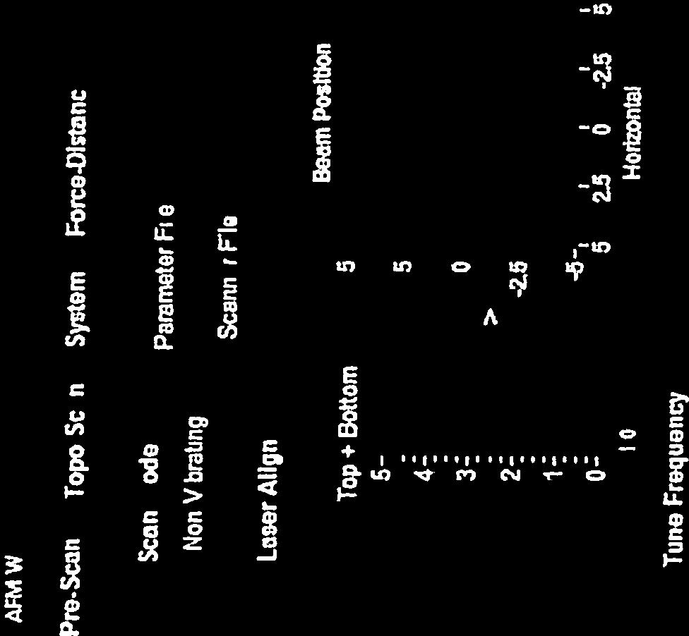
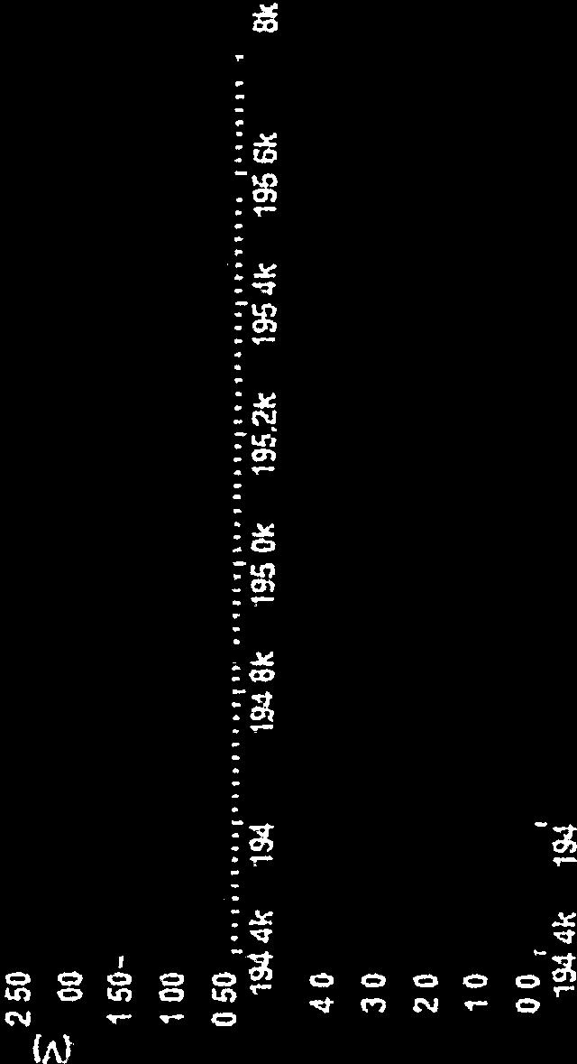
10 Tune Frequency The Tune Frequency window is used for selecting the optimal conditions for producing vibrating-mode images. There are two oscilloscope windows: the upper window shows the amplitude of the probe's vibration, while the lower window shows the phase between the drive frequency and the measured frequency. The variable controls are: 1. Amplitude and Phase sliders: Adjusting the amplitude scroll bar will alter the driving amplitude of the probe's vibration. Adjusting the phase scroll bar alters the phase degree. For optimal scanning, the amplitude should not exceed 2.5V or the resonance will become saturated (see section 5.4). 2. Lower, Selected, and Upper Frequency: The lower, selected, and upper frequencies correspond to green, blue, and red vertical bars in the oscilloscope windows, respectively. V 2.2 TT-AFM Users Guide Modes There are two TT-AFM modes: Vibrating mode and Non-Vibrating, or contact mode. The modes are selected with the Scan Mode button. When Vibrating mode is selected, the frequency sweep window is activated. When Non-Vibrating mode is selected, the frequency sweep window is deactivated. Scan Mode QJ Non-Vibrating Laser Align The position of the laser on the four-quadrant photo-detector is presented numerically and visually in the Laser Align window. These two indicators are both updated in real time and are used for aligning the light lever. There is a switch for turning the laser On and Off. This switch will automatically turn the laser off after the system has been inactive for a certain length of time. NOTE: After the TT-AFM light lever is set up for the first time (see Appendix A.6), the thumb screws used for laser alignment should not need to be turned more than a few turns. Laser Align Top+ Bottom 5: 4: 3: 2: Beam Po&lllon Laser Power Top- Bottom Left- Right 1133 Hortzontal

11 of the resonance peak and on the steepest part of the slope of the phase curve, owing to attractive and repulsive forces at work on the cantilever's oscillation. 3. Start and Stop: These buttons can be used to start and stop frequency sweeps. 4. Demod Gain: This function adjusts the gain used when driving the tickler piezo. 4dB is a good starting value for a reference sample, but should be altered in conjunction with the drive amplitude with different probes/samples to maintain a resonance peak under 2.5V. Ph (deg) 25: 360-; 2 ~ 300 ~ - _v_2_.2_ 1_ TT_-_A_F_M_u_s_e_rs_G_u_i_d_e -'_.fii!.piii The usable range of the piezoelectric scanner is measured with the Range Check option. When started, the scanner is moved in a square pattern, which can be readily observed with the video optical microscope. This function must be completed before beginning a scan. Start ~ Complete Range Check Range Check Up 1 Jog Size (microns) Down Speed ~~(ii' mm/sec ~[15.0 Manual Z Motor Control Esc j E-Stop 4 CAUTON: Always visually monitor the position of the Z motor. The Z motor can drive the cantilever into the sample stage and damage both the probe holder and the scanner. The Z motor, which raises and lowers the light lever, is activated with this window. The speed of this motion can be controlled with the speed slider. When the Up and Down buttons are held down the motor slews. The motor is jogged by touching the Up and Down buttons. The jog size can also be controlled. The E-Stop button is the emergency stop function, and can be accessed via the Esc button Manual Z Motor Control 1~ 0..5~ 100.;: o ~ ~ oll ;) "' ;.)f90oo DemodGain~ 1 5~ 200.:; When trying to find the resonance peak of a new probe, it is advised to set the lower and upper frequencies to the boundaries of the frequency of the probe itself, which should be located on the probe box. The selected frequency should fall just to the left

12 Automated Tip Approach The Automated Tip Approach button starts the process of the probe moving toward the surface. A woodpecker motion is used, which results in noticeable clicking sounds from the microscope stage. This sound is from two sources: the stepper motor being energized and the Z piezoelectric ceramic being retracted. When the system is engaged in feedback, the Open Loop button will light up and say "n Feedback." A small Adv button on the far right of the Z Drive range allows advanced users to manually manipulate tip approach, by altering the setpoint and jogging the Z motor. This can achieve a lighter feedback for high resolution scanning. See section 6 for more information on high resolution scanning Topo Scan Window Automated Tip Approach Automated Tip Approach Opm loop to-,llzonv. r,.d;l -to.: ~ : (V) After the Pre-Scan functions are ready, the Topo Scan window is used for measuring AFM images. -- j eoooaao=~ r.:<- J : ~ 1,... M A<N V 2.2 TT-AFM Users Guide.. CAUTON: Before activating the Range Check function, make sure that the probe is moved away from the sample surface. f the probe is too close to the surface, the probe may be damaged. : (V) ~_] ~ Setpoint{mV) 1730 n 10:1 Z_Enor Ft:~back O~ ZOrM: l...amplitude: _10;1 Jog Down j j 0.00 (um) ~

13 40.0 ];,.. 1 G. 20.0, ~ t i Grid OFf 4n.O ~r---~~~-----, 10.0 V 2.2 TT-AFM Users Guide SHC buttons on the right side of the mage Windows allow users to open the scans in a larger window and adjust the color scheme and histogram in real time. Each of the windows is opened by clicking on S, H, or C; the window can be closed by re-clicking on the s, H, ore. 40, mage Window Two images are displayed simultaneously while scanning. The type of images and their appearances are selected in the Display menu window. As the images are displayed, there is a constant normalization of the data so that the images appear in full scale.

14 The histogram (H) can be adjusted by moving the red and green vertical bars. The C button allows the user to choose between a number of color schemes. The S button opens a larger version of the image in a new window Oscilloscope Window AZ vs. X position plot of the probe as it scans across a surface is plotted in two screens. The data plotted is selected in the Display window. 100 i ~!i: -50 ~ o 1 o o o o o o o ' o o X Position (lim) X Position (J.m) V 2.2 TT-AFM Users Guide!

15 3. Scan Lines: The number of lines in the y-axis and the number of pixels measured in the x-axis. S<an Rate J07"" Hz E.:,.l Scan Unes f256 o.~.. - V 2.2 TT-AFM Users Guide 3. ntegral: Scale factor for the integral term in the PD feedback controller. Setpoint (mv) J 0 1. Gain: Scale factor for the feedback control signal. 2. Proportional: Scale factor for the proportional term in the PD feedback controller. ntegral ~ 1000 Derivative ~ 0 Reset to Config ] All of the parameters for maintaining feedback are provided here. The parameters are: Gain.;1] Proportional ~ Z Feedback ZFeedback 10. Zoom Box: This shows the position and size of the scan in a grid. The scan area must be within the zoom box area. 9. Scan Complete: This indicator turns green when a scan is completed. 8. Current YX Position: The position of the probe along the y-axis as a scan is taken at 0", along the x-axis for a 90" scan. 7. Center. The center of the scan in x and y coordinates. 6. Rotation: A scan can be completed with 0" or 90" rotation. 4. Scan Size: The range of the scan, from 0.1 micron to either 15 or 50 microns (depending on scanner size). 5. Samples/Pixel: The number of data points signal averaged per pixel while a scan is being taken. Scan Size rso ""' >- Samples/Pixelf"iO" Rotation r-cr- Center X 25 ""' y f25 ""' X posftion (~m) ~=~ ~m) Saln Complete Scan Setup All of the parameters required for scanning are presented in the Scan Setup window. Once scanning is started, these parameters may not be changed. The parameters are: 1. Type: The scan can be either 2-D, which scans just the x-axis, or 3-D, which scans both the x- and y-axis. 2. Scan Rate: The rate in Hertz that the probe is scanned across the surface (max 2Hz). Scan Setup Type (3D

16 4. Derivative: Scale factor for the derivative term in the PD feedback controller. 5. Setpoint: Parameter that controls the magnitude of interaction between the probe and surface Display CAUTON: f the Z Feedback parameters are too high, the Z ceramic can begin to oscillate and potentially cause damage to the ceramic. There are several options for changing the appearance of the images displayed in the Scan window. They are: 1. Left mage: The source of the image displayed in the left image window. 2. Right mage: The source of the image displayed in the right image window. 3. Background: When Line Leveling is selected, the background is subtracted from the image one line at a time. 4. Display: Two types of displays may be selected: Color Map and Light Shaded. 5. mage Add: This function allows the user to overlay the left and right images while scanning. The opacity may be adjusted by the % value. Display Left mage j Z_DRVE Right mage J Z_ERR Background Line Leveling Display J Color Map Add ~!} 0.16 Source of signals displayed in the "Display Left/Right" drop down boxes GPD ZAMP ZPHASE V 2.2 TT-AFM Users Guide.. mago ~ i'l ZERR ZDRVE ZSENSE

17 Tip Retract After scanning a sample, this function is used to move the tip away from the surface. The Tip Retract function should always be used to assure that the probe does not get damaged after scanning Scan These buttons allow the user to start and stop scans. Tip Retract Up ~ Complete Stop ] Scan V 2.2 TT AFM Users Guide System tab in vibrating mode System tab in non-vibrating mode ,_ 1~ 1 - ~ -:._a. ',_,... ~ - -f'i' - -1'"'...::.:P.i= 1 ~-~, l r- -'- 1~ 1 =R= r-r-;-- y... ~ ~ --G~,,... --ruo "' i"-"",~"'~"'frioo'--._,... ~ rrr-,...,... ~ 1 :::c 1 --r--.=.:j? "'--F" le.p!m,- ~ The system tab has several parameters that control the functionality of the TT-AFM. These parameters should not be changed without a detailed understanding of the function that is being modified. ncorrect use of the system functions can damage the TT-AFM System Window

18 Tip Approach This sub-window controls the step used for the stepper motor in tip approach. These functions are very useful for high resolution imaging (see section 6). The Tip Approach motor jog value automatically adjusts to changes in the Z HV Gain (reduces by a factor of 1/3rd). When the advanced tip approach options are not selected on the Pre-Scan tab, the Tip Approach motor jog function moves to the Other Controls sub-window Z Parameters ~Appro.cft r.--ten TpApGal" ~ 20000,,... :r-..- TpAp """"' ;,f10oo TpAp Dtnv.tift -ro- Tl p AppG PD~ &!:tnd hdor f.l o.eoo Rctracto.ttl~ FHdbRkDtted ~...-:omo- Vibrating mode values Tip~,.,... TpApGoi» fto'oo,..._... :r-;;- TpAf!lnt.p~,... r-;- '"'""'~ ExtlllldD. roro; Rebe<tDeh~ FmlbKitDaeet~ Non-vibrating mode values The high-voltage amplifier that drives the Z ceramic in the ZPamneters XYZ scanner has 15 gain settings. This function allows reduction of the Z gain of the high-voltage amplifier. Reducing the Z S«tuo r Gi in~ ZHV Ga in~ gain reduces the dynamic range of the ceramic, which also reduces the noise floor of the instrument. & NOTE: A new high voltage gain value is entered into the system when tip approach is being undertaken. Without enabling tip approach, the Z setting will not change XYZ Calibration The calibration values in this sub-window can be adjusted when scanning a standard reference sample. Appendix C explains how to calibrate the TT-AFM in detail. NOTE: Changing the calibration values will change the scale on images measured with the TT-AFM. Only change the values when calibrating with a reference sample. NOTE: The Save button will turn green when pushed. However, the new values will not be saved in the Scanner configuration file until the Exit button is pushed in the Topo Scan window. The user must have administrator rights in order to save the calibration values. calibration X_ cal ; v_cal ; Z_cal,.lr----- ~ Save 1 V 2.2 TT-AFM Users Guide

19 the X and Y ceramics, which can be used for measuring and reducing Z noise in images (see Appendix D for instructions on how to complete a Noise Floor). XY HV Gain allows gain reduction of the X and Y high-voltage amplifiers, similar to Z HV Gain. Reducing the X and Y GPD settings will decrease strain gauge activity. This will affect linearization, but will also reduce the noise floor of the system Other Controls X Proportional ~ 256 Xlnteg<al # 4096 XDerivatiw ~ Y Gain(%) ~ 100 Y Proportional ~ 256 y lntegal ~ 4096 vo.-.. j}l XYHVGain ~ 15 - V 2.2 TT-AFM Users Guide Other Controls for vibrating mode Other Controls for non-vibrating mode feedback limit ro:or- Ttp Approuh motor jog (lim) ~ lip Approach motor jog~ fftdbfl:khma r;:o:;- ~ ~plitude~ l..amplitude f'ojs7 EdendOdtt ~ 8uperEn1ble ~OFF S.VeConfigSettings ~ SlveConfrgSettings BeeperEMblc goff ~ Other Cont rols 6. Tip Approach motor jog: This function will appear in the Other Controls sub-window when the advanced tip approach options are not visible. 5. Extend Delta: This function determines the amount of probe deflection on the surface in non-vibrating mode. Extend delta is typically 0.1, meaning the Top-Bottom signal will deflect by 0.1V before feedback is initiated. 4. Extend Factor. This function determines the percent decrease of vibrational amplitude of the probe in vibrating mode. The typical range for extend factor is , with 0.95 creating a 5% reduction in vibrational amplitude for high resolution scanning. 3. Feedback Limit This function controls the feedback LED that turns green when Tip Approach has achieved feedback. f the feedback light is flickering when the tip is in feedback, increase this value by 0.01V. 2. Amplitude Value: Displays the current Z amplitude used in Tip Approach. This value should correspond with the Selected Frequency on the Pre Scan tab. 1. Beeper. Enables a beeper that notifies an operator that a scan is completed with an audible tone. (Speakers must be enabled) XY Parameters Adjusting these parameters will alter the voltages applied to X Gain(%) ~ 100

20 3.2.4 Force/Distance Curves Force/distance curves are created by measuring the deflection of the cantilever as the sample is moved towards and then away from the probe at the end of the cantilever. The shape of a F/D curve depends primarily on the cantilever stiffness and the thickness of a surface contamination layer. For information about how to analyze F/D curves, see Appendix. Measurement of F/D curves is found on the Force-Distance tab. The AFM must be in feedback in non-vibrating mode before a F/D curve is measured. There are three important parameters that must be set before the F/D curve is measured. They are: 1. Down: The distance in nanometers that the sample will be moved away from the probe when the F/D curve measurement is initiated. 2. Up: The distance in nanometers that the sample will be moved up from the feedback position during the F/D curve. During this part of the curve, the probe is touching the sample surface. 3. Rate: The rate or velocity of the sample as it is moved towards and away from the probe. v'.... _. -- \} ;1 =rr:::::: V 2.2 TT-AFM Users Guide..

21 - 3.3 Video-View Software The video optical microscope software allows real time visualization of the probe and surface. The software also allows for real time capture of both images and videos. Operation of the video software requires substantial computer processing speed; when computers with slower processing speeds are used, the image can often change contrast. The change in contrast is triggered by other programs using the computer's processing capacity. Below is a brief description of the function found in the software package. t is recommended to optimize the parameters for each type of sample. Before operating the video camera, it must be properly aligned; see Appendix A. G.rm~: ---{}- ~ Gait ---{} R i]--- 5Zl G:;}- 500 Sao..atm Q ~ 0/biC(: 0 ~ ~ OeldOsetSa DllsetY:O UoaX 0 0 ejshowrebclt ~ ~ - 1 ~ Many of the video camera's adjustments can be accessed by selecting the P for parameter settings. These adjustments include exposure, contrast, gamma, gain, and offset in X and Y. The software also allows users to measure features on the screen, cell count, and export their screen captures to Excel or Word. See the tool bar below. The quality of the image viewed with the video microscope depends directly on the reflectivity of the sample being viewed. Therefore, it is not possible to give instructions for optimizing the video microscope images. t is recommended that operators experiment to find the best parameters. V 2.2 TT-AFM Users Guide t File View Video mage Musure Cell count Setting Advanced H!lp lct:i 0 o a ~ C D llil ll Lrl o fa + 0 ~ 2043'1536 ~~'iii x "" «> ls lti:l L ll !!!!!! " 1.- /~ D 0 & 0 0:: 0 Jt t ~ (j) (j) w A R N Ci 0 Oofd UoaY 0 - ~ Defd.Relidlloc B.-1]-- n9 QroQst ---(}- ~ []RNQoneAE EPOUe:..-{}--- - ~

22 4. Focus Adjust: The user can manually alter the microscope's focus with these z-motion adjustment knobs. NOTE: f the operation of the video optical microscope does not seem familiar, please review the contents of Appendix A, section 2. _v _2_.2_ t_ TT_-_A_FM_ u_s_e_rs_g_u_l_de fib.!!ip Measuring mages With the TT-AFM Once the TT-AFM is assembled, users can expect to take a few hours to learn how to measure images. t is very important to learn how to: 1. Operate the video microscope. 2. Prepare samples. 3. Exchange probes. 4. Align the light lever force sensor. 5. Perform video-microscope-assisted tip approach. Once these techniques have been mastered, measuring images is relatively simple. 4.1 Operating the Video Microscope Operating the video microscope is essential for efficient operation of the TT-AFM. t allows for proper viewing of the sample, assists in manual tip approach, and is critical for laser and photo-detector alignment. t is advised to practice operating the video microscope before attempting to replace probes or measure images. The components of the video microscope are: 1. XY Position Translator. At the base of the support pole are XY position translators used for centering the probe in the video microscope window. 2. Zoom Adjust: The zoom lens allows for viewing of a surface at high or low magnification. The light intensity must be adjusted when using the zoom lens. 3. Light ntensity Adjust: t is often critical to adjust the intensity of the light on a sample to get the best image. (not shown)

23 4.2 Preparing Samples Metal disks serve as sample holders for the TT AFM. Attach the sample to a metal disk with double-stick tape or glue. Once a sample is attached to the disk, it is held onto the microscope's sample holder magnetically. t is critical that the sample be tightly bound to the sample disk in order to avoid vibrations, which degrade the image resolution Exchanging Samples Follow the steps below to successfully exchange samples with the TT-AFM. 1. Raise the Z motor until the probe is at least Y." from the sample's surface. 2. Remove the probe holder (see section 4.3). 3. Place the sample disk on the top of the sample holder. Adjust with small, sharp tweezers until the sample is visible in the video microscope. CAUTON: Do not place excessive force on the sample holder, as it could break away from the piezoelectric ceramic. 4. Align the sample using the video optics (see section 4.1 ). 5. Replace the probe holder with the probe tip facing the sample. ltmii!!.!.@ v_2_.2_ 1_ T_T-_A_F_M_u_s_e_rs_ G_ui_de

24 7. Once the new probe is positioned correctly, place the probe holder back into the microscope. NOTE: f the probe holder does not sit completely level with the probe exchange mechanism, it is possible to adjust to the screws on the bottom of the exchange tool to achieve the desired height. _v_2_.2_ 1_ TT_-_A_F_M_U_s_e_rs_G_u_i_de._ il.!i@ifj 4.3 Exchanging Probes When a tip becomes damaged or broken, these steps can be followed to exchange probes quickly and efficiently. NOTE: Make sure the new probe is close at hand and facing in the same orientation as the probe exchange tool. 1. Raise the Z motor until the probe is at least Y." from the sample's surface. 2. Remove the probe holder from the light lever. 3. Place the probe holder on the probe exchange tool with the spring facing up. 4. Push down on the probe holder, such that the spring releases the probe. 5. Tap the probe exchange tool lightly on a flat surface at a 30" angle until the probe slides down through the narrow channel of the exchange tool. Gently dispose of the old probe with tweezers. CAUTON: The exchange tool will not prevent expulsion of the probe if the tapping angle is too extreme. 6. Using the tips of very sharp tweezers, pick up the new probe and, while pressing down on the probe holder, gently slide the probe into place. Take care not to touch the cantilever with the tweezers.

25 4.4 Aligning the Light Lever Force Sensor Aligning the light lever force sensor is greatly facilitated by understanding the optical path of the light in the sensor. The following figure shows the light path and the effect of turning the adjustment knobs on the light lever. Gain Switch Motion of the red dot in the Pre Scan window when the detector adjust knobs are turned clockwise Tips for aligning the light lever force sensor Motion of the laser spot when the laser adjust knobs are turned clockwise. 1. Bringing the cantilever within a milimeter of the sample's surface can help the user see the laser on the sample. 2. f the cantilever does not align within a few minutes, try another cantilever. 3. After replacing a cantilever, the laser and photo-detector adjustments are usually less than a single turn. 4. The adjustment screws have backlash; sometimes the motion is not perfectly linear. 5. The detector has two modes: high and low gain. High gain allows more laser light through the detector than low gain. High gain is commonly used for most scanning purposes because it has a better signal to noise ratio. 6. When in vibrating mode, if the resonance peak appears inverted at the top, reduce the amplitude slider. f further adjustments are necessary, switch the detector gain from high to low. 7. f the Beam Position is not aligned within a few turns of the adjustment knobs, the photodetector can be manually adjusted by loosening the set screws holding the detector down and repositioning the detector so that the Top + Bottom signal is maximized while the Beam Position is mostly centered. V 2.2 TT-AFM Users Guide

26 4.5 Optically-Assisted Tip Approach Tip approach with the TT-AFM is achieved using a woodpecker algorithm activated in the Pre-Scan window. To save time during tip approach, move the probe as close to the surface as possible before activating the Automatic Tip Approach function. The video microscope can prove very helpful for manual probe approach. Below are two images of a probe as it moves toward a standard reference sample surface Perform optically assisted tip approach 1. Focus the video microscope on the sample surface. 2. Carefully lower the Z motor with the Manual Z Motor Control, or manually with the motor knob, until the cantilever is visible in the video microscope image. Make sure the Jog Size has been set to a low step size and the Z motor speed is set to 0.00 mm/sec in order to avoid crashing the probe into the sample. 3. Slowly jog the probe down until it is only slightly out of focus. 4. As the probe approaches the surface, a second laser spot will appear on the surface if the sample is reflective. Once the second laser spot merges with the spot on the cantilever, the tip is flush with the surface. This effect is useful for judging the distance from the probe to the sample. V 2.2 TT-AFM Users Guide Tip Far Away From Suface Sample Tip Near Surface CAUTON : f the tip touches the surface before the feedback is activated, the tip may be damaged or even broken.

27 4.6 Contact Mode maging These instructions assume the AFM-View software is properly loaded and working, and that the material presented in section 4 has been reviewed Pre-Scan Tab 1. Follow the instructions in section 4.2. and place a sample in the instrument. 2. Follow the instructions in section 4.3. and place a contact mode probe in the instrument. See Appendix E for probe recommendations. 3. Focus the video optical microscope on the AFM probe. 4. Follow the instructions in section 4.4. to align the laser on the probe. Make sure the Top - Bottom signal is between 0.4 and 0.8 for contact-mode imaging. 5. Select Non-Vibrating in the Scan Mode window. 6. Focus the video microscope on the sample surface. 7. f this is the first scan since opening the AFM-View software, click on Start in the Range Check window f ~1. NOTE: The probe must NOT be in contact with the sample surface during Range Check. The piezoelectric ceramics will move to measure the usable range, which may cause damage to the tip. Use the Manual Z Motor Control to move the light lever towards the sample (see section 4.5.). nitiate Automated Tip Approach. Wait for the green light to indicate that feedback was achieved. f the Z Drive indicator is above the center of its range, click the Adv button and use the Re-Center function. f the Re-Center function does not initiate a new tip approach, increase the setpoint value by 1 OOmV. f the Z Drive indicator is below the center of its range, click the Adv button and jog the motor up by small increments until the indicator is at the center of the Z range. 12. Once true feedback has been achieved, open the Topo Scan tab at the top of the AFM Workshop window. W!!.J.F-' V-2_.2_ /_ T_T-_A_F_M_U_s_e_rs_G_ ui_de

28 5 ) _v_z_._z_ J_T_T-_A_F_M_ u_s_e_r_s_g_u_i_d_e Mi!.iifHii j Top Bottom j Left-Right 250 ~,,. ~150 J1oo 0 ~s4 4k. '-i94'gk.. 'i94' 6k... ;gs Ok. "i95.2i.:' 'i954k"' 196Sk'" i~ 8k 40 f" :20 ~10 0 1~4k t 1~Bk t~ok 1ss'2k 1954k 1iSGk 195Sk Fr«p.~nty(:Hz) 7 Pre-Scan J Topo Stln ~ System J Fof'C.()stance } Top+Botlom 5: -- 4~ J~ 2~ ;ll '"' Tune Frequency A~tudl - (Vpp) (d : 2i :;oo: 1 s~ 200' 1~ 0 5~ o;.., 100,] F~nc:ySeloct DemodG.bn 4dB 8

29 4.6.2 Topo Scan Tab 1. Select scan parameters such as Scan Size, Scan Rate and the number of lines. Samples may be scanned at o or go by adjusting the Rotation parameter. NOTE: A scan rate of 0.5 Hz and 256 scan lines will achieve a basic low resolution scan. 2. Select the desired images to be displayed in the Display window. The Display window also allows for control of leveling, as well as the ability to transpose both the Left and Right mages with the mage Add button. Some display options for contact mode scanning include: Z-Drive, the change in voltage through the z-piezoelectric ceramic, shows the sample's topography. t is common to set Z-Drive to the Left mage. Z-Error, the error signal, is used to help optimize the Z Feedback parameters. When initially setting up a scan, it is common to use Z-ERR as the Right mage. L-R, lateral force, detects cantilever torsion as the tip applies constant force along the surface. This mode is unique to contact mode scanning, and can only be properly used when scanning at go. 3. Begin a scan by pressing the Start button in the Scan window. NOTE: When the GPD parameters are optimized, the Z piezoelectric ceramic will more closely follow the probe tip as it scans the surface. When tip movement is minimized the Z error signal is decreased. ncreasing the setpoint by small increments ( mv) sharpens the image by pushing the tip harder on the surface. 4. While scanning, optimize the GPD and setpoint parameters (see Appendix G). 5. Once the parameters are optimized, stop the scan by pressing the Stop button. 6. Before beginning a new scan, check to see if Z Drive is still near the center of its range. f not, see sections Begin a new scan. When the scan is completed, the light turns green. 8. f desired, the user can open a larger window of both the Left and Right mages by selecting the S button to the right of the scan window. The H and C buttons allow the user to alter the histogram and color scheme of the scans, accordingly. g. When finished scanning, press Tip Retract. This function lightly releases the probe from the sample surface. ll:h f!.\.i_. v_2_.2_ 1_ T_T-_A_F_M_u_s_e_rs_ G_u_ide

30 0.0,,,,.,., JO XPositlon(llfTl) ,...,...,..,..,., 500.co.o r,.,. flil SCin FUte ros- Hz Sein Lints f'ts6 :Jf :S """""' rsr-...! Se""'-f'O" Rolltioor;o:- C..UJXr;s... lvf25 ""' ~ t - 21)75 ~ ~300! ~"' -' > ,,...,..,.., X Position bun) 8ackgrot.lnd J Linelevehr1{1 Display Color Map -=e~ ~ - _v_2_.2, _rr _._A_F_M_ u_s_e_rs_ G_u_id_e ii!.! M 6 2

31 4.7 Vibrating Mode maging These instructions assume the AFM-View software is properly loaded and working, and that the material presented in section 4 has been reviewed Pre-Scan Tab 1. Follow the instructions in section 4.2. and place a sample in the instrument. 2. Follow the instructions in section 4.3. and place a vibrating mode probe in the instrument. See Appendix E for probe recommendations. 3. Focus the video optical microscope on the AFM probe. 4. Follow the instructions in section 4.4. to align the laser on the probe. Make sure the Top -Bottom signal is close to 0.0 for vibrating mode imaging. 5. Select Vibrating in the Scan Mode window. NOTE: The probe must NOT be in contact with the sample surface during Range Check. The piezoelectric ceramics will move to measure the usable range, which may cause damage to the tip. 6. f this is the first scan since opening the AFM-View software, initiate the Range Check function. 7. Select the frequency under the Tune Frequency window. a. Set the Lower limit to the lowest frequency on the probe box. b. Set the Higher limit to the highest frequency on the probe box. c. Set the Selected value to any frequency between the two limits. f the selected frequency exceeds either limit, the software will automatically change the values. d. Set the number of steps (50-100) and the Demod Gain (4dB). e. Scan the frequency. f. Move the green and red cursors toward the resonance peak to decrease the range, and place the blue cursor corresponding with the selected frequency 80% up the left side of the resonance peak. g. Repeat steps (d) and (e) until a resonance peak no greater than 2.5V is observed. f the amplitude of the resonance peak exceeds 2.5V, adjust the driving amplitude of vibration by altering the Amplitude scroll bar. h. For phase mode imaging, the resonance peak must correspond with the slope of the phase curve. To alter the phase degree, adjust the Phase scroll bar accordingly. 8. Focus the video microscope on the sample surface. 9. Use the Manual Z Motor Control to move the light lever towards the sample (see section 4.5.). 10. nitiate Automated Tip Approach. Wait for the green light to indicate that feedback was achieved. Mt8i!!.ng v_2_.2_ 1_ T_T-_A_F_M_u_s_e_rs_G_ ui_de

32 11. f the Z Drive indicator is above the center of its range, click the Adv button and use the Re-Center function. f the Re-Center function does not initiate a new tip approach, increase the setpoint value by 1 OOmV. 12. f the Z Drive indicator is below the center of its range, click the Adv button and jog the motor up by small increments until the indicator is at the center of the Z range. 13. Once true feedback has been achieved, open the Topo Scan tab at the top of the AFM Workshop window f't>.s..n l Topo S..n ) s,...m j F.,...o...,e j, ~ f PerameterFde J C:\Uws\AfMUsel\tl<e1ktop\2.0J-50Mic,ooAFM\'/Olbhop\dltl\fm_defult.dg :, ~- &annet File f C.\UsenWM lhet\desktop\2.0.3 SO Miaoo AFMWOJbhopW.t.\suooc,_defult.dg La~erAtlgn 2;,, '; Amplitude (Vpp) ~5~ 2~ Pho,. (deg) 360: 300' 1.5~ 200' 1~ 100.: 0.5~ o= ~,] ro;oo rrooo "'""""" Frequency Select ~ Low.,('H:r) j S<Ud{ktlt ~ UJ~P«{tH ).. floo ttumsteps ~ DemGd Gtio j4d9"' ~ fl.o Spetd JogSiu(micnms),~{'000 FsO mmjsec i2.0 ~ ~.4k k t!u.bk 1!i.Ok 195.2k t95.4k ts5.61t 1!JS.Bk Frequency (l!hz) Esc~ AutomatedTipAppmach Setpoint(mV) 0 z..<= l..amptitud ~ 0.00 (um) 11 '12 _v_2_.2, _rr _ -_A_F_M_ u_s_e_rs_ G_u_i_d_e!!.J.iliil... ]

33 4.7.2 Topo Scan Tab 1. Select scan parameters such as Scan Size, Scan Rate and the number of lines. Samples may be scanned at o or 90" by adjusting the Rotation parameter. NOTE: A scan rate of 0.5 Hz and 256 scan lines will achieve a basic low resolution scan. 2. Select the desired images to be displayed in the Display window. The Display window also allows for control of line leveling, as well as the ability to transpose both the Left and Right mages with the mage Add button. Some display options for vibrating mode scanning include: Z-Drive, the change in voltage through the z-piezoelectric ceramic, shows the sample's topography. t is common to set Z-Drive to the Left mage. Z-Error, the error signal, is used to help optimize the Z Feedback parameters. When initially setting up a scan, it is common to use Z-ERR as the Right mage. Z-Phase, phase imaging mode, uses the differences in the probe's oscillation to form image contrast. The phase shifts when the probe comes into contact with areas of the sample surface with differing stiffness, adhesion, etc. Thus phase imaging mode is optimal for composite samples, those with varying surface densities and characteristics. 3. Begin a scan by pressing the Start button in the Scan window. 4. While scanning, optimize the GPD and setpoint parameters (instructions in Appendix G). NOTE: When the GPD parameters are optimized, the Z piezoelectric ceramic will more closely follow the probe tip as it scans the surface. When tip movement is minimized the Z e rror signal is decreased. Decreasing the setpoint by small increments ( mv) sharpens the image by pushing the tip harder on the surface. 5. Once the parameters are optiized,stop the scan by pressing the Stop button. 6. Before beginning a new scan, check to see if Z Drive is still at the center of its range. f not, see sections Begin a new scan. When the scan is completed, the light turns green. 8. f desired, the user can open a larger window of both the Left and Right mages by selecting the S button to the right of the scan window. The H and C buttons allow the user to alter the histogram and color scheme of the scans, accordingly. 9. When finished scanning, press Tip Retract. This function lightly releases the probe from the sample surface. lt4i6".!1!-' v-2_.2_ 1_T_T-_A_F_M_u_s_e_rs_G_ui_de

34 _V_2_ _T_T_ _A_F_M_ U_s_e_rs_ G_u_ld_e..J_ffii!.J. MW {1211 1~~><-! ,. o: M : ZDrive. Display J CoiD'Map ~ ~ ;)Oi' Ruottoeo..., j o~o io'.o ~ ' ' 20.0 JOO '40.0 X... (Jmol.:,...,...,...,...,...., nsetup , XPolltlon{J.un)

35 5. Troubleshooting - What Can Go Wrong When Measuring mages Although the operation of the TT-AFM is quite simple, some problems can occur while imaging samples. The following sections detail some of the most common problems that may occur. t is important to keep these potential problems in mind when operating the TT-AFM. 5.1 Saturation of the Photo-Detector Highly-reflective cantilevers can sometimes pass too much laser light to the photo-detector. When this occurs, the light lever force sensor will not work properly. When there is too much light, the Top + Bottom signal in the Laser Align window displays a value greater than 3. This problem can often be solved by flipping the gain switch on the photo-detector down to low gain (see section 4.4 for the location of the gain switch). 5.2 Sample Not Mounted Correctly t is essential that the sample is rigidly mounted on the sample holding plate. f the sample is not mounted rigidly, it can be difficult to get into feedback, and images appear to have excessive vibrations. 5.3 Probe Not Seated Correctly f the probe is seated correctly, it will be in essentially the same place before and after the probe is removed from the AFM. f it is too difficult to align the light lever after a probe exchange, examine the probe holder closely to make sure that the probe is seated correctly. mproper probe alignment may cause resonance saturation. V 2.2 TT-AFM Users Guide

36 5. 7 Defective Probe n the event that none of the above problems exist and it is not possible to get an image, the probe may be defective. _v_2_.2 1_T_T_-_A_FM u_s_e_~_g_u_i_de ~~i@h flhihi}ii _:-"",;.. oj: ~= ,.., _... ~, --, _,---:... ~ ~.-..,- 5.4 Resonance Saturated When scanning the frequency of the cantilever produces a double-peaked resonance, as shown on the right, decrease the driving amplitude of the probe by lowering the Amplitude scroll bar until the resonance peak sits below 2.5V. f the resonance is still saturated, the probe may have to be re-seated. 5.5 False Feedback n vibrating mode, the probe can go into false feedback, resulting in wispy, featureless images. False feedback is created when the probe is caught up in the surface contamination layer. This can be corrected by activating the tip approach function a second or third time, as well as by utilizing the advanced tip approach functions to jog the tip toward the surface (see section 6). 5.6 Scanner at End of Z Range When the Z ceramic expands or retracts to the end of its range while scanning, the image will suddenly lose contrast and appear flat. To solve this problem, relocate the sample so that the area being scanned lies directly over the center of the z piezo, (the screw hole of the sample holder). Next, redo tip approach so that the Z ceramic is in the center of its range (see section 4.6. j-k).

37 6. High Resolution maging High resolution images are measureable with the TT-AFM. However, as with any AFM, obtaining those images requires that the AFM be optimally set up and that the operator knows the critical parameters for measuring high resolution images. The table below illustrates the difficulty in measuring images as a function of the desired dimensions. very hard hard easy : Nanometer.. -. ; "" t '..., -._.. '.. l.. "''..; "., r 1-3 nm Test Particles 0.3 nm Si Terraces 1.2x1.2 1Jm Tobacco Mosaic Virus ~. -~.=~ :~<i''., _,. _.!;;.. '. '... '..._... ("7- ' ' ~-.. ;,~~~ }-.- #'~. '.:i.h'.o;.:...,_, _bw,,. v._...:.. _. '...-r" ~ - -~"'"'.:; 2x2 1Jm ndium Tin Oxide V 2.2 TT-AFM Users Guide. :-, )". Examples of high resolution images obtained with the TT-AFM include:,...,.. \ '.' ,,. :... -.:..... '... -,....,.~... ~-.. ' ~...,, _,,.... <~"'...J.,. ~. ' ~ ~... _ '. :'... \. ~. ' ' ~ i ".,.,,!"~. _, ~-.0::. - -~ : ',.. ~:.._~,_,...,' ~--.:... ~ : ~-~,,. t '. -~ ~-.. ~ '....::-~:-~, ,~ ~~ -~ : : - ~.~ J:.

38 _v_2_.2_ J_ r_r_-a_f_m_ u_se_rs_ G_u_i_de,_!t.!!ipfi There are three critcal requirements for measuring high resolution images with the TT-AFM: 1. The instrument must not be influenced by structural and acoustic vibrations. For high resolution imaging, the AFM must be placed in an environment with minimal vibrations. Typically, both a vibration table as well as an acoustic enclosure is required. Often measurements must be made in the middle of the night when there are minimal structural vibrations. Measuring the noise floor of the AFM establishes the Z resolution of the AFM. Measuring images of structures with 0.3 nm in vertical dimension requires a Z noise floor below 0.1 nm. See Appendix D to learn how to measure the noise floor of the TT-AFM. 2. The Electronics Gain must be properly set up. The scanner used for the measurements must be cabable of resolving the desired features. The resolution of the scanner depends on the electronic noise in the control electronics and the mechanical gain of the piezoelectric ceramics in the scanner. n the TT-AFM the electronic noise can be reduced by reducing the Gain on the high voltage amplifiers that drive the scanner piezolectric ceramics. Alternatively, use a scanner with a small mechanical gain. The 15 micron scanner has a mechanical gain of 1:1 and the 50 micron scanner has an XY mechanical gain of 5:1. Theoretical resolution for 151Jm and S01.1m scanners 501Jm Scanner 151Jm Scanner Z HV Gain Z Range (nm) Z Noise (nm) Z Range (nm) Z Noise (nm)

39 - As lower Z high voltage gains are used, the maximum Z range decreases. Therefore, the step size of the Z motor must be reduced when lower Z gains are used. This will assure that the probe does not crash into the sample surface on tip approach. The software automatically adjusts the tip approach motor jog for changes in the Z HV Gain. 3. Tip approach must be made such that the tip is not broken. Preserving a sharp tip for imaging requires making a perfect tip approach. This means that the probe must not crash into the surface and break the tip off. The best method for preserving the tip in probe approach is to bring the tip to the surface and engage in a false feedback. Then, very gently bring the tip into feedback such that the tip is interacting with the surface. The following graph shows the interaction forces of the probe with the surface. Distance There are 4 regions of interaction forces between the tip and surface: No interaction force Acoustic interaction forces nteraction of the tip with the surface contamination Direct interaction between the probe and the surface. These interaction forces will cause the vibrating cantilever to decrease in its amplitude as it passes through each of these interaction regimes. The method for getting into perfect feedback is to stop the tip approach in the green regime, and then slowly bring the probe into the direct interaction regime. This is achieved by setting the feedback threshold low such that the tip approach stops when the probe is interacting with the surface contamination (Extend Factor< 0.9). Then the probe can be slowly jogged towards the surface using the advanced tip approach functions. The user will know when the tip has entered the direct interaction regime when the yellow Z Drive slider no longer moves as the sample is pulled toward the tip via small setpoint changes. The AFM control software is designed to make a careful probe approach under manual control. This is achieved with the Advanced Tip Approach window under the Pre-Scan tab in conjunction with the Tip Approach Parameters window under the System tab. if:hjif,@-' v-2_.2_ /_ T_T-_A_F_M_U_s_e_rs_G_ui_de

40 The initial value for the setpoint when feedback is established is the Z Amplitude multiplied by the Extend Factor. -A!pruch~ T~OM ~ '"""'-~ """... :floio '"'""""' :ro """pgf'd~ Start V 2.2 TT-AFM Users Guide Automated Tip Approach Stop 1 1 Setpoint (mv) Z_Error Jog Down 1 ) 0.00 {um) Re-Center 1 j Fixed Set Pt l 1730 n 10= O.OOO Feedback 0 ~ Z Drive 1 Adv 1 Z...Amplitude o-'l ;j : (V) Jog Up GPD Z Piezo Light Lever Force Sensor Tip Approach Sequence in Vibrating Mode Step Description Result Tip Approach Parameter Measure vibration Amplitude used for initial Z Amplitude value in amplitude of the probe tip approach. Setpoint is the Automated Tip away from the surface. raised and lowered around Approach Window this value which causes the sample to move up and down. Raise setpoint. Z piezo moves toward the Extend Factor probe. Check for feedback. f in feedback, end tip Feedback Detect approach. Lower setpoint. Moves sample away from Retract Delta probe. Activate stepper motor. Moves probe towards Tip Approach Motor Jog sample. Repeat steps 2-5. Feedback achieved with full Z Drive range t is advantageous to move the sample up and down towards the probe at a slow rate to avoid crashing the probe into the surface. The rate at which the sample moves up and down depends on: The magnitude of the initial Z Amplitude Tip approach GPD parameters Extend Factor Retract Delta

41 - Appendix A: Setting Up the TT-AFM A.1 Selecting a Location Structural vibrations from a building's floor and acoustic vibrations can greatly reduce the resolution of an AFM. deally, the AFM would be placed in a vibration-free environment, but this is typically not possible. A few tips: Set the AFM up in the basement or lower floor near a bearing wall. Avoid setting the AFM near fans or other sources of wind turbulence. Avoid locations where there are elevators, a lot of foot traffic, or freeways. f you must place the AFM in an undesirable location, consider purchasing a vibration table and/or acoustic enclosure. A simple test to see if a location has a problem is to fill a coffee cup with coffee and set it in the potential location. f there are ripples in the coffee's surface, there are going to be problems. A.2 Setting Up the Optical Microscope The video optical microscope is essential for efficient operation of the D-AFM.After setting up the microscope, we recommend spending some time learning to operate it by viewing some samples. 1. Assemble the Video Microscope a. Attach the X-Y translators to the base. b. Attach the post to the X-Y translator through the small adapter piece. c. Place the Z translator on the post and tighten. d. nstall the zoom tube and CCD camera. e. Attach the USB cable to the CCD and computer. f. Attach the LED to the zoom tube, and connect the light power cable from the LED to the light intensity adjuster. g. Remove the black cap at the bottom of the zoom tube. V 2.2 TT-AFM Users Guide

42 V 2.2 TT-AFM Users Guide WARNNG: Failure to connect the ground wire can cause damage to the stage and/or Ebox electronic circuits. WARNNG: Always turn off the master power to the Ebox before plugging or unplugging any of the cables on the TT-AFM. 60-pin Ribbon Cable 2. Test the microscope and verify its operation. a. Launch the Video View software (see section 3.3). b. Turn on the light and adjust the intensity to its mid-range. c. Adjust the height of the zoom tube so that the bottom of the tube is 115 mm from the surface of the table. d. Place a coin or other metal object under the objective. The light should be visible on the object. e. On the zoom tube, turn the zoom adjustment counter clockwise all the way, thus reducing the magnification. f. At this time, an image should be visible on the computer screen; use the focus adjust on the video microscope to sharpen the image. g. ncrease the magnification with the zoom tube adjuster and increase the light intensity as needed. A.3 Connecting the TT-AFM to the Cables 1. Connect the USB cable between the computer and the Ebox. 2. Connect the 60-pin ribbon cable between the Ebox and the TT-AFM stage. 3. Connect the grounding wire between the Ebox and the TT-AFM stage.

43 A.4 System Check 1. Turn on the computer and the Ebox Launch the AFM View software. Using the Manual Z Motor Control in the Pre-Scan tab, move the Z motor a few steps. 4. f the Z motor does not respond and the Top-Bottom numbers in the Laser Align section of the Pre-Scan tab are not flickering, the Ebox is not communicating with the computer. n this case, cycle power to the Ebox and restart the AFM View software. A.5 Aligning the Video and TT-AFM Microscopes 1. Raise the zoom tube on the optical microscope so that the light lever can fit under the bottom of the zoom tube. 2. Move the micrometers on the video microscope XY translators to their central position. Move the micrometers on the TT-AFM stage to their central position. 3. Place the TT-AFM stage under the zoom tube such that the hole in the light lever is directly below the zoom tube optical objective. 4. Adjust the height of the zoom tube so that the bottom of the tube is about 115 mm from the top of the AFM sample holder. Move the stage by hand and adjust the optical focus. 5. Place a probe in the probe holder (see section 4.3.) and place it into the light lever. 6. With the Z motor control, move the probe such that is about Y. in. above the sample plate. 7. With the focus adjustment knob, raise the zoom tube approximately Y. in. 8. Slowly move the stage by hand until the probe is viewed in the video microscope window. As required, adjust the focus, the lighting, and the position of the stage until the probe is in the center of the optical view V 2.2 TT-AFM Users Guide

44 Move the laser spot out to the edge of the cantilever. Set screw holding Release the set screws that hold the photo-detec- photo-detector tor in place. ~ Move the photo-detector in and out until the T-8 signal is zero. Tighten the set screws. Move the L-R signal to zero by adjusting the detector translation thumb screws. V 2.2 TT-AFM Users Guide ~~-. ~'": ~~,, rn -.. -~ ~ : ~~,} J A.6 First Alignment of the Light Lever This procedure assumes that the light lever was correctly aligned at the factory or by an authorized agent. 1. Place the sample disk on the sample holder. 2. Place the probe holder in the light lever with a contact or vibrating mode probe installed. 3. Adjust the optical microscope until the probe/substrate can be viewed on screen. 4. Center the laser and detector translation mechanisms with thumb screws. 5. Turn on the laser. 6. Use a flathead screwdriver to rotate the mirror until the laser spot is on the back side of the cantilever. 7. Lower the Z motor until the probe is just above the sample disk. 8. Rotate the mirror to move the laser light until it is visible on the probe. 9. Loosen the set screws that hold the laser. 10. Slide the laser in or out until it is focused. 11. Tighten the set screws to hold the laser in place.

45 A. 7 nstalling the XYZ Piezoelectric Scanner 1. f not already turned off, turn off the Ebox electronics. 2. Place the scanner on the TT-AFM XY translator and locate the ribbon cable that plugs into the scanner. 3. Plug in the ribbon cable. The connector is located on the back of the scanner. 4. Screw in the three socket screws that hold the scanner onto the XY translator. A.8 Leveling Sample Holder CAUTON: Do not twist the ribbon cable. Doing so will damage the TT-AFM electronics. The leveling sample holder allows the user to better adjust the tilt of the sample being scanned. To use, simply place the leveling sample holder on the regular sample holder on the scanner, aligning the magnets. To adjust, tighten or loosen the three adjustment screws on the leveling sample holder until proper leveling is achieved. A.9 Grounding the TT-AFM There are several grounding options for the TT-AFM. The green ground wire should be used to connect the stage with the Ebox. The probe is grounded by a grounding connector, which should be attached to the Modes/10 connection on the back of the stage. A wire can be added to the ground connector to receive signals from the probe. V 2.2 TT-AFM Users Guide

46 Position - 0 Jog s1ze (um) 15.0 [Tune Frequency] Ampl1tude (V) Phas e (deg) ~ 90. oo Lower Freq ~Hz~ m:~t~~e~re~z (H;) 1 ; 5 m963 Num steps 100 Tune per1od (ms) 500 HPP!~~~oi~~t~~~lb Ga1n 2048 T1p Approach NoV1b 1 Proportional ~ 64 i~ ~ :c~~~:~~ ~g~~ ~ ~~~~e~~ ~ v; ~og T1 p A.pproach v1 b 1 Ga1 n 1024 Proport1onal T1p A.pproach v1b T1p Approach v1b ntegral o scan Nov1b Ga1n scan NOV1b 1 Proport1onal ~ 100 scan Nov1 b 1 ntegra scan NoVib Derivative "" 0 scan vib 1 Gain '"" 2048 scan vib Proportional scan v1b 1 ntegral 1000 scan v1b oer1vat1ve - o V 2.2 TT-AFM Users Guide scan type - 1 state - o f1 rst_f1 ag 0 new_line_scan_data - 0 curre nt vertical Position (um)... o. 000 line_index ~m_ l~~:le s :-~~?ggo Y...A um Y_B um - o. 000 line_de ta scan_rate (Hz) - o. so s 1 ze (um) - so. 000 points_per_bin- 20 oemod Gain - 4 Laser control - 1 Rotation - o Feedback_L imi~ - o. 040 [o1sp1ay] Left mage - 1 Right ma~e - 2 g~~~~~~u~ 0-1 Left Pallet - 4 Right Pallet - 4 mage Add " mage Add sw - o Appendix 8: TT-AFM Files The TT-AFM software uses three separate files. The first is a parameter file which stores all of the parameters used for operating the microscope. The second is a scanner file, which is unique for each scanner and has range and calibration information. Finally, data files contain images measured by the microscope. Parameter File C:\Users\AFM User\Desktop\ Micron AFM Workshop\data\afm_default.cfg Scanner File C:\Users\AFM User\Desktop\ Micron AFM Workshop\data\scanner_default.cfg 8.1 Parameter Files When the AFM-View software is launched, the default parameter file is used to set all of the parameters that are displayed on the screen. A new parameter file may be created from the default parameter file and stored with a different name. The new parameter file can be loaded in the Pre-Scan window. Below is a list of all of the functions in the parameter file. f"'11**"*"*** **~~~'* "'*.,.* -. - rr-so Micron * AFM workshop * - Atomic Force Microscope - configuration F1le Jan. 4, 2013 i:~~9~:mi_~ath.. "Test Data" Testda'ta...fil e_ext - "wsf" ~~a=~~:~i~-p.g~h "Diagnostic'' oegug_f 1 ag - o ShOVJ Adv.- "1" scan_comp 1 e'te_\'jav.,. "windows XP shutdown. wav" [scan Mode] scan Mode.. o [system Control] T-B_OFF a 0 xvz_relay_wait_time scan Rate limits- 2,2,2,2,2 samples/ Pixel 11m1'ts - 25,25,25,25,25 [Motor] or1ve ( %) - so Acceleration (mi crosteps/ seca2) 1000 velocity (microsteps/ sec) [Tip App values] TipApp_Novib_ext_del~a TipApp_NOVib_ret_del~a TipApp_NoVib_feedback_de~ect TipApp_Novib_ext._~imeou~ TipApp_Novib_ret_timeout TipApp_vib_ ext_factor T1pApp_v1b_ret_de1ta TipApp_v1b_feedback_detect TipApp_vib_ext_timeout TipApp_vib_ret_timeout TipApp_mo-cor_jog_'t.imeout""" 3.0 [Tip Retract values] Tip_Re~_NoVib_ret_del~a Tip_Ret_Novib_ret_timeout 60.0 Tip_Re't._Vib_ret_del~a Tip_Ret_vib_ret_timeout: Tip_Ret_update_time_ms Tip_Re~_motor_jog_um Tip_Ret_motor_jog_timeout 3. 0 [Z Pi ezo sett:i ngs] Z HV Gain - 15 z sensor Gain [XV Piezo sutings] XV Acceleration xv velocity - o XV HV Gain - 15 X sensor Gain - Y sensor Gain - [scann1ng]

47 8.2 Scanner Files Every scanner has its own corresponding file. These files have the calibration and range information used by the AFM-View software. The contents of the file for the 50 and 15 ~m scanners are: ~***~******************************* - * TT-50 Micron * = AFM workshop Atomic Force Microscope scanner File Jan. 4, 2013 [system nformation] S stem_seria1-~o. = 0 F1rmware_Rev1s1on = 0 OAQ...Serial_No. = '" '" [Range check] Max Y = [Cal size] [calibration] [XY Positioning] x offset = 0 Y offset = 0 x.._oerivative = 0 Y_Oerivative = Data Files ~**************** ****** ********** *** * TT-15 Micron * AFM workshop Atomic Force Microscope scanner File Jan. 4, 2013 [system nformation] S stem_seria1-~o. = 0 F1rmware_Rev1s1on = 0 DAQ.._Seri al_no. = '"18F9A1E'" [Range check] [cal size] Z_Range (um) = 8 [ca 1 i br ati on] [XY Positioning] x offset = 0 v offset = o x...oerivative 0 v_oerivative = 0 TT-AFM data files are stored in a text format. At the top of the data file are the parameters used for the scan. Max x = Min X= Min Y = Margin (%) = 3.0 cal size (um) = Zoom Box ncrement = 10 Range span (counts) = Z_Range (um) = 17 x.._cal Y_cal = z_cal = x scale = 1 v scale = 1 [XY Piezo control (GU)] JLGain{%) = Y_Gain(%) = JLProportional = 256 Y_Proportional = 256 JLintegral = 4096 Y_ntegral = 4096 V 2.2 TT-AFM Users Guide Max x = Max Y = Min X= Min Y = Margin{%)= 3.0 cal size (um) = 15.0 zoom sox ncrement = 3 Range span (counts) = x...cal v_cal = z_c:al = X scale = 1 Y scale = 1 [XY Piezo control (GU)] X...Gain{%) = Y_Gain{%) = X...Proportional = 256 Y_Proportional = 256 X...ntegral = 4096 Y_ntegral = 4096

48 l. oi ~~. ~ ~ 1 ~. will- w... n.,_,,-a'' 2.40 U<l "" 1 1. = ljl 0 (1LlOO.C9Dirm~lJSlrm V 2.2 TT-AFM Users Guide tl 0 11& 255 llli l.l! ~ ljs, ljj ll! ~... [im] llj 2.B '-- ""' r--a 1'-- '- ~ L..-' v 10 lo JO., " ~~ GiLl Appendix C: Calibration Calibration of the TT-AFM requires scanning a standard sample that has known X,Y and Z dimensions. f a sample with squares is used, the pitch in X and Y should be around 10 )Jm. The height of the features in Z should be around 100 nm. 1. Scan a standard sample with known dimensions in X,Y and Z in both X (0 ) and Y (90 ). 2. Open the AFM Calibration software. Make sure to allow blocked content. New X: NewY: NewZ: ~ iiw] o 3. nsert the current calibration values, located on the System tab, under System Cal in the calibration software. 4. nsert the known values for the calibration standard in the Actual column in the calibration software. 5. To calibrate X, open the completed oo scan in Gwyddion and level the image. 6. Extract a profile over the nicest row of squares, in this case, and click Apply.

49 Using the Measure Distances feature on the bottom left-hand corner of the extracted profile, create vertical lines that bisect each square at approximately the same poin -c~ Mdbod: lh~ Poiots X[llfll] Y[nm] l.tri!jill[~ml Hright[nm],..[deg) 9.85D1l.S !.7... U BJl JV... Ol.., 2.38 l!l!l 2) " "' ~ ~ f'w- "' ~~ iu U8 0 " \_,J RJ [JJil8'l~rl """U!67'm ~ ~ ~ nsert the values in the Length column into each X Measures blanks in the calibration software. New X : NewY: New Z : x(!1fl] Updlle Cnlibrations D V 2.2 TT-AFM Users Guide '-...! v ~ ~! 20 ]Q Gnph 1Dm C~nt~

50 V 2.2 T-AFM Users Guide g. Repeat steps 5-8 with the completed go scan to obtain Y Measures values. Make sure to extract a profile along the best looking column of squares in they-direction. ll ~.ill ~ ll ~~ ll ~~~ ~s ~Q ~bl '!lpm,ldju~ -tiijnm ~ JJ 1J 1J ~.~ l lll ow m ~ > ~.~.1},70 <Op&os llnl M 30 ~ ~ ~~~ 10. To calibrate Z, the user may either use the o or go scan. Extract a profile, and measure distances from the top of each square to the bottom of each pit. Enter the Height values in the Z Measures blanks in the calibration software. ( -_, x 1, - OX C~ncl

51 - 11. Once the calibration software is completely filled out, select Calculate to obtain the new calibration values. Enter these values in the System tab and click Save. New X : New Y : New Z : Updote Cclibrctions D Calibration X_cal Y_cal.}-cal Save ] CAUTON: Do not twist the ribbon cable. Doing so will damage the TT-AFM electronics. NOTE: To obtain the most accurate calibration values for the scanner, the user may have to complete multiple calibration iterations. V 2.2 TT-AFM Users Guide ~J ~J ~J

52 Crop the data, if necessary. lu Level the image by pressing the Level Data by Mean Subtraction button, and the Correct Lines by Matching Height Median button. Find the noise value with the Statistical Quantities button, under Ra (Sa) for surface roughness. V 2.2 TT-AFM Users Guide Appendix D: Noise Floor To measure the noise floor, it is necessary to scan the sample with no voltage applied to the X and Y piezoelectric ceramics. The AFM-View software can measure the structural noise of the system when the tip is in feedback with the surface. 1. Make sure the tip is a sizeable distance from the surface. nitiate the Tip Retract function, if necessary. 2. Under the System tab in XY Parameters, change the value of the XY HV Gain to zero. This shuts off the voltage to both the X and Y ceramics. 3. Under the Topo Scan tab, set the scan parameters for noise measurements: Scan Size = 0.5 Jm Scan Rate = 1 Hz Scan Lines= 512 X,Y Center= (2, 2) for 50 Jm scanner, (0.5, 0.5) for 15 1Jm scanner Left, Right mage = Z-Drive, Z-Error 4. Using the Manual Z Motor Control, move the probe toward the sample until the probe begins to come into focus. 5. nitiate Automated Tip Approach. 6. Begin a scan. t is not necessary to complete a whole scan; 50 scan lines is plenty. 7. To analyze the noise floor measurement, open the completed Z-Drive scan in Gwyddion.

53 - 10 f ile: ;dit ~olumedata nfo. ~ El G raph. R ~ ~~ ill Slze O.Onm O.Onm W.dth 129.9nm Exclude mnked region QptioM ~ lnrtjntupdates E~ P' E~ px ~~a ' E EJ px P..rameters 9 8 Mu:imum: -l09.302nm """' -(1,0418 Su1hcearea: 6.78Sx10'lSm~ ProjectedarN: 6.469:o:10'15 m2 Noise can be reduced by lowering the Z HV Gain in the System tab. When the Z gain is lowered, a new tip approach must be initiated because the Z ceramic's dynamic range has been reduced. ij J V 2.2 TT-AFM Users Guide CAUTON: ncreasing the Z HV Gain will increase the Z ceramic's dynamic range, and will raise the sample stage. Make sure the tip is removed from the surface before increasing Z HV Gain. (104.8 nm. 0.7 nm): nm."1". '" lbo 1100 ~ [_~date : [ &le~j ~ 0 nclude only mnked region -211» 0 Use entire image {ignore mask) Height 49.8nm nm Origin ~ ~ l;;? ~ )J.. &Wt ~~ ~.fj' ~ nclination&. O.Odeg lnclinationcp: deg Rms(Sq]' 0.213nm Rms (grain-wise): OlUnm Kurtosi5: 2.1B Ra(Sa): Ol..56nm Minimum: nm Median: nm Avu4gevalu1!: nm

54 CM28-A probes from Applied Nanostructures recommended. V 2.2 TT-AFM Users Guide Appendix E: Probes There are two major types of probes, vibrating mode and non-vibrating mode probes. Each of these probes may have a coating, which makes them more reflective. 1. Vibrating Mode (VM) Probes Vibrating mode probes are in the shape of a rectangle. Typical VM probe specifications: Resonance Frequency khz Length micron Width micron Thickness micron Force Constant N/M TM190-A or ACLA probes from Applied Nanostructures recommended. 2. Non-Vibrating Mode (NVM) Probes Non-vibrating mode probes can be in the shape of a V or rectangular. Typical NVM probe specifications are: Resonance Frequency khz Length micron Width micron Thickness micron Force Constant N/M

55 c: 0 :;:; ns E...E c: ns (J c:.c: (J ~ u...~ "C c: Q) c. c. <( ' c E~ "' Cl Q) o.s::... o ~ o:z Clu. ~.s:: 0... :2 ; - c f/).0 :::~..!!! Q) "iii >.cu ~ ~... o cu - :S(ii - 0 cu c e= 1ij:g ;:: <(.s::. o:z -;;;< Q)U. c;;t-! ~1- Q) cut-!.s::t -o.s:: c... Q).S:: a.s: a.~ cu c ~:8 ~--~ V E E Cl ll i5.x (,) 0 ffi (,) ;: (,) Q) iii... u.: la!t AiD 40 1 var, Ga V Hlfl<n1> ~ D G!lli~"O: ~--- ~;: 150 \' ~ ' '! i\oc :.. iioc ADC M C D<C i\dc ADC AOC -----~ ~ ~ -! : Gon1rol linog G! MOt<:< j, ~ (-C ~====~~~Z~SG~n~~~======~ T ~ - 24 BT VD ~c r.,: ~==- Notes: 1) ADC lines are shared 2) All control lines are from the micro controller 3) ADC, DAC, 1/0 from National nstruments Card l C) --ru;.e,.:indff nl ~.. P,U.>;P,DC M:x! PtOzO 1 ell "C :; (!)!! ell ll :::> ::!E u. <(...:. 1- N.,; >.~ Q).. i\uxi\dc:t c:ru '- c E ~.E c ~ cu.5 :8.0 > 0 Q) : SCU<:r 1-.5: <( -~ m E c ~ 0 ~ ai

56 17 G18 ] _1_ V 2.2 TT-AFM Users Guide 6, s, REF ACy - ~ 6, g. REF AC~, E71 ~ LZR Pv\'R ~ 4 1 ;; 4$ _;; 49_;::: o 6-o.,-o 8-<J.{"') 9.n 10.;:; u.;:.. 12 _;::: B.Q o n;: &.(; 19.;.. 2C.{;.,., ~ 21.;:; ;:: -o ;! -o -" -C'l -~..(') 26...() 2'i 1 ;., 2&.0 29.;: :, -o ~1 ::: -o ""...(') 34.;; 35 _;; :7 -o ~6 3a -o ~go-o 40.Q " _roo, 41 4"~ -o 4:: -o "-Cl 44.{') 45...() 45-l"l.. R.;::F E125 -:;:: F.2 Ebox and Modes Pin Assignments 13, 3 X SE~SE ~ 1 13, 3jx REF - 3, 9 X DRVE 3, 3 ' y SDtSE ' 13, 3! Y P..EP 0, 3 Y DPJVE B Z SDlSE 7 11, 1!, 1 3,,4 Z DPJVE 1, 12, 4 Z_ERR " 12, 4 Z S.ET 13, 6, Z,:\MP'L., - - : 13, 6 Z PH.. ~SE ' 12, 13, 5 T-B 12, 5 L-R 12, 5 "l'+b 2, 13, 4,. Z D.-\C / 2, 13 ( At.'X ADC 1 L 12, 13 < AL'X _:::o..rn.;_.2 ' L B, Sl' TC.bK

57 Appendix G: Optimizing GPD Parameters The Z feedback scan parameters, such as the setpoint voltage and the GPD parameters, are adjusted as the line scan is being made. The goal for adjusting these parameters is to have the probe perfectly track the surface. The probe is tracking the surface when the Z error image has a minimal signal. Establishing the optimal conditions requires practice and some intuition. When first learning to operate an AFM, it is helpful to scan a reference sample in 20 and adjust the GPD settings to see the effect on the Z voltage and the Z error signal, as shown in the figure below. S9ltings F""dbo!tk ali Feoobaclo; "perf;,d" ' Elf act l]) loo;- pily - 7 Result on image l D_1 l)eflecuon Hllignt L~~~- Oeflll(:loon ~V\J- H9ighl ~~.r LlLf Hcighl Ocflodion OefleG1ion l D_1 He'lJ1l V 2.2 TT-AFM Users Guide

58 V 2.2 TT-AFM Users Guide i O<Yim and lntertam fj' N USB-6l090EM2 ""' '. ''.1-b.1 Network Dvim ~ SoH ffi Scales 'fl TffiPan~s. Software ~ ResotO<Yico ole Systems ~ CroaloTask... <$ Configuro TEOS. Rona me H~p ~ Self-Calibrate ' " Value Ox19JDJ40 955f4 Appendix H: Renaming National nstruments DAQ Device The following procedure will allow the user to reset the National nstruments DAQ card registry with the device number corresponding with the user's Ebox. This may be useful if the user's AFM-View Software does not initialize. Open the Nl MAX: Measurement and Automation Explorer software as follows: file Edit View Took Help ~-t.lj-~ 1> :i Data Neighborhood ~> idev~ctsilndlnttrfm:s ~ Scales ' /)lsoftwnt 1 9Romo~ Syuru National nstruments Measurement & Automation Explorer ~l easurement &Automation Explorer (LAX) prcmdts access to )our NaUonat lflstuments prodocts. <{ What do you want to do? l.lanagem} de\1cesandml~rfam 61 Uanage m1 mstatled Nationaltnsiuments soltkaje l!l ManageY!tJJalehannetsortasl:sformrde'Aces ~ Createscalesformy\utuaiJnslruments 8 Con~gure my M insbument driv!t5... tmportlexporfmyd!liteco'fi~uruonfite 1. Expand Devices and nterfaces under My System on the left scroll tab. 2. Making sure the correct Ebox USB is plugged into the computer, delete any devices that are not green. There should only be one green device, corresponding with the DAQ card in the user's Ebox. 3. Rename the only remaining green device as Dev1. This can be accomplished by right-clicking on the device and selecting Rename. File Elf~ Vii!W Tools Hap ~ My Sy~em - -= ===='====Jr:~=== ~ [i Data N~ghborhood Name S<f=.T=ffi==~=T=ffi=P=an=ols=... =~==R.,=ot=O=..,=."=;J

59 - V 2.2 TT-AFM Users Guide n a light lever AFM, the user must convert the T-B signal into the cantilever deflection. This is achieved by measuring the change in the T-B signal as the sample is directly pushing against the probe. This is labeled slope data in the first figure above. The force constant for the cantilever is supplied by the manufacturer. K = force constant d = deflection of the cantilever Force=- K * d The deflection of the cantilever can be converted to Force using Hook's law: What is actually measured is the deflection of the cantilever, or the Top- Bottom (T-B) signal of the photo-detector. Appendix Analyzing Force/Distance Curves A force/distance curve is a graph that shows the amount a cantilever tip bends as it is systematically pushed into a sample. The probe may be lowered onto the surface, or the surface may be raised into the probe.

60 The force/distance curve from the TT-AFM is illustrated in the figure below. The data is measured using a TM 190-A probe from Applied Nanostructures on a hard silicon surface. Data was analyzed using an industry standard spreadsheet program. The blue line shows the curve measured as the samp[e is moved towards the probe, and the red line is the curve measured as the sample is pulled away from the probe '1.15 T-B(V) '1 ' Blue - Sample Up ~1: Red - Sample Down ~~~ ~\)~~ 11 3'1 5' '11' '123" )1 32' The spring constant for TM190-A probes in 40 N/m. Thus, to calculate the adhesion force from the data in the figure above: Fad = (( v) (.05 v/nm)) * 40 nn/nm = 7.2 nn V 2.2 TT-AFM Users Guide ~ppendl'<: 59 ~ -' "1~\4....., - 1--:- ~ - -