ezafm OPERATING MANUAL

Transcription

1 ezafm OPERATING MANUAL 2013rev 2.0 1

2 Table of Contents CHAPTER 1:ezAFM Introduction System Components Unpacking and Packing the Instrument Before Installation Unpacking the Instrument Installing ezafm Software Storing the Instrument Packing the Instrument CHAPTER 2:Measurement Installation Making the Connections ezafm Software Setup and Configuration Installing the Cantilever Selecting Cantilever Compatible Cantilevers Installing Cantilever Preparing Sample Mounting Sample ezafm Reference Samples CHAPTER 3:First Measurement Preparing the Instrument LEDs on the Controller Cantilever Tuning Approaching Starting a Measurement Finishing Measurement Saving the Image CHAPTER 4:ezAFM Software Advanced Dialogs Photo Diode PID Control Z Motor Control

3 Auto-Tune XY Offsets Scan Image Dialog Operating Modes Contact Mode Imaging Lateral Force Microscopy ( LFM) Tapping Mode and Phase Imaging Magnetic Force Microscopy FD Curves Cut and Rescan Color Palette Image Processing D Image Ruler Options CHAPTER 5:Improving Imaging Quality Laser Power Adjustment PID Adjustment Oscillation Amplitude Mechanical vibration noise Electrical or light noise Judging tip quality CHAPTER 6:Optional Modules Manual Sample Stage Signal Access Module Problems and solutions Quick Start Tapping Mode Quick Start Contact Mode Quick Start MFM Mode

4 CHAPTER 1: ezafm 4

5 1.1. Introduction The NanoMagnetics Instruments ezafm system is an atomic force microscope that can measure the topography and magnetic features of materials in nanometer scale. This system consists of a scan head which is operated using the ezafm controller and software System Components Components may vary depending on the configuration of the system. Typical components are shown below. Refer to invoice for particular contents. 1. ezafm with Vibration Isolation Unit 2. Controller 3. ezafm Cable 4. USB Cable (2) 5. Power Cable 6. Flash disc 7. User Kit 8. Signal Module ( optional) Figure 1- ezafm components 5

6 1.3. Unpacking and Packing the Instrument Before Installation Minimum computer requirements to operate the ezafm : - Windows 7/8 (32-64 bit) - 2 GB RAM - Free 2 USB 2.0 port By design, the ezafm is resistant to environmental vibration. For optimum performance it is still best practice to install the system in a suitable workspace. Ideally, a stable table or desk that is far from building vibrations, working pumps, electrical fields and air circulation should be used as a work station. Assure a well-grounded power supply is available to avoid electrical noise, a line filter is not required but may be used Unpacking the Instrument The system will be delivered in a fitted carrying case. Upon receipt, inspect the system components and promptly contact your NanoMagnetics Instruments representative should there be any damage. Prior to software installation it is necessary to connect the Controller to the computer for installation of the USB drivers. - Place the electronic controller unit on a stable table or desk and connect to main power using the supplied cable. Using the flat multi-pin ezafm cable, connect the controller unit to the ezafm scan head. Connect USB-B connector of both supplied USB cables to the appropriate port on the rear of the controller unit as shown in Figure 2. Figure 2- ezafm connections - Place the vibration isolation unit on controller making sure that the edges of the isolation system don t touch the controller and that it freely floats. 6

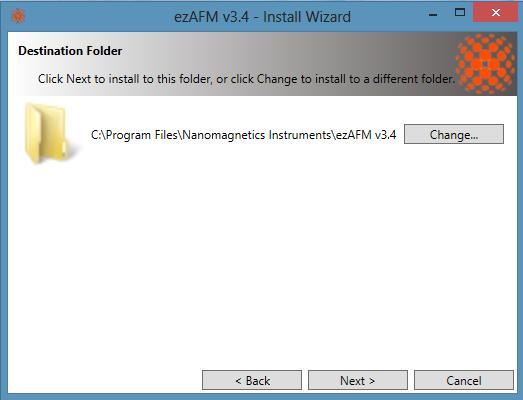
7 Figure 3- ezafm with vibration isolation unit - Place the ezafm scan head in the middle of the vibration isolation unit Installing ezafm Software - Before starting installation, make sure the cables between the USB ports and the computer are connected and switch on the power to the controller unit. - Insert the flash disc. - Open folder to view files. 7

8 - Install the ezafm software by double clicking EzAFM Setup Launcher. - Select Next 8

9 - Select Next - SelectNext 9

10 - Select Install - Select Finish and software will be launched Once both the electronics and the ezafm software are initialized, system drivers will be automatically installed. The ezafm software requires Microsoft.NET Framework 4.5 software. If not on the system computer you will be prompted during the ezafm software installation of the need for installation. For convenience, a setup file is included with the ezafm software. Please double click and start to installation. 10

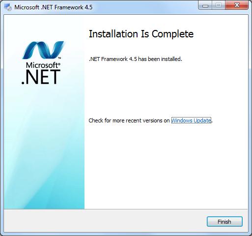
11 - Select Install - Select Finish 11

12 Storing the Instrument To avoid damage, for storage it is advisable to retract the cantilever to a safe position and then close software and shut off controller. Cantilevers may be left mounted in the instrument. When not in use it is preferred to leave an empty sample holder attached to the ezafm to protect the cantilever and holder Packing the Instrument Every main item has a fitted location in the instrument case. To protect the components, assure all cables are detached and put each item is stored in the proper location. Figure 4- ezafm package content 12

13 CHAPTER 2: Measurement 13

14 2. Installation Making the Connections - Make sure that the controller is connected to main power with power cable. - Connect the controller to ezafm with the ezafm multi-pin cable. - Connect the controller to the system computer using the supplied USB cables. Insert one each of the USB-B cables into the Camera and PC USB ports on the rear of the Controller. Insert opposite end of each cable into an available USB port on the system computer - Locate the vibration isolation unit to a suitable surface and assure that it is floating. - Place the ezafm scan head on the top of vibration isolation unit. Figure 5- Installed ezafm 14

15 WARNING!!! To avoid damage to the scan head, both shipping support pins MUST be removed prior to use as shown in Figure 6. Figure 6- Removing shipping support pins The pins are designed to lock the head in place for safe transportation. The pins may be reinserted for transport by selection of the Go to Park Position option in the Options menu which will align the scanner and allow for the pins to be replaced to the shipping position ezafm Software Setup and Configuration - Install ezafm software as detailed in Section 1 using the supplied flash disc, install the software. For each mode of operation a unique Serial key must be entered into the ezafm program. The keys are located in the Serial key text file located with the installation software. Additional scan modes may be added at any time by the purchase of mode specific Serial keys. Upgrades are completed using the same process of entering the Serial key text in the appropriate prompt within the software interface. 15

16 - Select and open Serial key text file. - Copy the key for the desired mode. - Paste the key into the window and select OK. 16

17 WARNING!!! To avoid potential damage to the scan head, calibration data must be entered prior to use. - Click Options on the top of the screen, select load calibration and load the calibration file located on the flash disc. Figure 7- Loading calibration file from the flash disc - Select Load Calibration and load the calibration file found on the software flash disc through a double click of the.txt file. - Select OK to acknowledge installation of calibration file and close the Options window by selecting X 17

18 2.2. Installing the Cantilever The ezafm uses a self-alignment system so there is no need for traditional alignment of the laser beam or photo detector adjustment. This feature allows the cantilever to be installed, removed and reinstalled quickly. The alignment system has an alignment chip with structures that correspond to matching the grooves at the back side of the cantilever. Care should be used to avoid contamination of the alignment chip as debris may interfere with proper cantilever positioning. In the event of contamination, the alignment chip may be cleaned using isopropanol and lint-free swabs. Compressed air or nitrogen gas may be used to remove loose debris from the alignment chip. Figure 8- Nanosensors alignment chip with alignment grooves Selecting Cantilever Cantilever selection is made based on operating mode. For dynamic mode, harder and shorter cantilevers, for contact mode more flexible and longer cantilever are suitable. For magnetic measurements cantilevers must be magnetically coated Compatible Cantilevers Compatible cantilevers for ezafm must have alignment grooves. These types of cantilevers are readily available from manufacturers such as Nanosensors, Budget sensor, Nanoworld, Applied nanostructures and Vista probes. Nominal length of cantilever must be at least 225 µm and 40 µm width Installing Cantilever There are two methods available for cantilever exchange, Manual and Auto Cantilever exchange. 18

19 Manual - Invert the ezafm scan head to gain access to the alignment chip. Figure 9- Inverted ezafm Thread thumbscrew into the tapped hole at the bottom of the scan head until the spring loaded fulcrum tension is released and there is sufficient access to the cantilever. Figure 10- Relieving fulcrum tension - Use supplied cantilever tweezers to select cantilever. 19

20 Figure 11- Select a cantilever - Place the cantilever on the alignment chip. Figure 12- Mounting the cantilever - Assure that the cantilever is properly seated by gently tapping the cantilever face with tweezers. Care should be used not to displace the cantilever or damage the tip. If there is movement of the cantilever it may be necessary to place the cantilever again. - When placed correctly, the equal reflection on the cantilever and alignment chip side walls will be visible. Also, small triangles between the back of cantilever and alignment chip will be visible. - Release the spring tension by removing the thumbscrew. 20

21 Figure 13- Mounted cantilever Auto-Cantilever Change An automated cantilever exchange process is available to simplify the replacement process through software control of the alignment chip position and spring loaded fulcrum. During the Change Tip process the laser is powered down and the fulcrum is opened to facilitate exchange. To initiate the process, select Start Change Tip from the Change Tip tab of the Home Page. Select Yes to initiate operation. Once selected, the laser will automatically power off at which point it will be necessary to invert the scan head as prompted by the program. 21

22 Select OK Once selected the scan head will move to the open fulcrum position to allow for the exchange of the cantilever. Exchange cantilever as detailed in the Manual Exchange process above. Once the cantilever has been exchanged, select Yes to return the scan head to service. This will retract the alignment chip to an operational position and power up the laser. Check the laser position on the under main Page->Approach Tab->Photodiode from ezafm software. When the cantilever is correctly indexed in the chip carrier the laser location on photodiode will be indicated as near to center in the Photo Diode display as shown in Figure 14.If the cantilever is properly indexed within the alignment chip, it is possible to vary the laser power between 0 and ~4V. Prior to tuning the cantilever adjust the laser power to ~3V through adjustment of the slider under the photodiode window. The FN and FL should be smaller than 2V, if not the cantilever should be refitted assuring proper location. 22

23 Figure14- Photo diode window NOTE: Numeric values and position indicated in the Photo Diode window do not need to be absolute Preparing Sample For all types of AFM, sample preparation is an important step. For optimal resolution, substrate selection should be considered based on sample size and composition. Substrates should be chosen considering your structure sizes. For example to image small particles such as nanoparticles or nanospheres, anatomically flat substrates such as mica, silicon should be chosen. For large sample structures such as cells glass may be used as a substrate Mounting Sample Once sample preparation is complete it is necessary to mount it to an ezafm s sample holder. The ezafm sample holders are manufactured of magnetic stainless steel which is held in place magnetically. Double sided tape, glue or silver paint may be used to attach samples to sample holder. Please be sure that sample properly attached to sample holder. If not it may damage the cantilever when you mount the sample. 23

24 - Place double sided tape onto the sample holder. - Remove the non-adhesive backing from the double sided tape. - Place sample on tape. Maximum sample size is that which fits within a 10mm diameter circle up to 5mm deep or a 7x7x5 mm square. - Mount the sample holder at the bottom of ezafm which will be held in place magnetically. - Make sure your sample is under the cantilever by looking through the viewing port on the ezafm. Figure 15- Mounting a sample using double sided tape 24

25 ezafm Reference Samples Included with each ezafm system is a number of reference samples including: Gypsum (Hydrated Calcium Sulfate): Gypsum is a very soft natural mineral with the chemical formula CaSO4.2H2O. Atomic steps are visible using a 10x10 µm 2 scan area as shown in the following image. Figure 16-10x10 µm 2 AFM image of gypsum mineral - iphone 3GS CMOS Chip: This sample is 3.2 MP camera s sensor chip manufactured by Omni Vision Tech. Period of the sample is 1.7 µm and height of each structure is 400nm. This sample may be used to check XY and Z calibration. Figure 17-20x20 µm 2 AFM image of iphone 3G CMOS chip 25

26 - Bluray DVD section: Bluray DVD s area optical disk storage device which has a 320 nm track pitch. Scanning 10x10 µm 2 area will reveal data storage bits as shown below. Figure 18-10x10 µm 2 AFM image of Bluray DVD - Hard disk Sample: This sample is useful when using the MFM option. Magnetic bits on the surface are shown when scanned at 10x10 µm 2 areas. Using the multiple scan image channels available, it is possible to see the difference between topography and MFM images with 100 nm lift off. Figure 19-10x10 µm 2 AFM image of hard disk sample. Topography (left), MFM phase shift (right) 26

27 CHAPTER 3: First Measurement 27

28 3.1. Preparing the Instrument Prepare the instrument as described in section 2. Select and install a suitable cantilever for the mode in which you want to operate the system. Prepare a sample and attach magnetically to ezafm LEDs on the Controller There are four LEDs on the front face of the controller. 1. Power LED: Controller is switched on. 2. PC LED: ezafm controller connected to computer. 3. Cam LED : ezafm controller connected to computer 4. Status LED : White LED: Software connected to ezafm controller Blinking red LED: Scanning a sample Blue LED: Motor is moving, cantilever is being tuned, getting F-d curve etc. Green LED: Approach is done. Figure 20- Led on the ezafm controller 3.3. Cantilever Tuning The cantilever must be tuned any time the software is started, the ezafm power cycled or physical changes made to the cantilever. Through this process the ezafm is tuned to the specific resonant frequency of the cantilever. This is an automated process in the ezafm software with the exception of setting the expected frequency range of the cantilever. Prior to cantilever tuning assures that the laser voltage is approximately ~3.0V as described in section

29 Default values are preset to bracket the resonance frequencies of standard cantilevers (PPP-NCLR). If alternative cantilevers are used, adjust the starting and ending frequencies found within the Auto-tune window by clicking button. Using the Excitation slide in the General window, adjust the percentage to approximately ~10% and select Auto-Tune option. Once the Auto-tune has completed the Oscillation Amplitude should be adjusted to approximately ~2.0V using the Excitation slide. Auto Tune dialog on the General tab (Figure 21) tunes the cantilever automatically but not shows the resonance curve of cantilever. The last resonance curve is accessible all the time Within the Auto Tune window as in Figure 22. Figure 21- Auto tune dialog Within the Auto Tune window, confirm the shape generated in the RMS curve displays a smooth Gaussian shape with the peak approximating the resonant frequency of the cantilever as shown in Figure 20. There is also Start (Hz) and End (Hz) textboxes that you can adjust frequency sweep range if you are using a cantilever which has a resonance peak in a different frequency range. Figure 22- Auto tune graph 29

30 3.4. Approaching To scan a sample, the tip of the cantilever must be extremely close to the sample surface. Great care during approach is required. There are two types of approach; manual and automatic. Manual: If the cantilever is positioned far from the sample surface you can choose manual approach to decrease the spacing between tip and sample. To approach, lower the arrow on the approach bar. You should observe the distance between cantilever and sample through the window on ezafm or onboard video camera, to assure that the cantilever will not touch the sample thereby damaging the cantilever or potentially the sample surface. During approach the blue led will illuminate on the controller. To halt approach, press the Stop button on the left. When the approach is done blue LED will turn to green. Figure 23- Course approach form Fine adjustment is possible by single steps by pressing Approach or Retract button. You can adjust the step size by moving up or down the arrow on the approach bar. Automatic: To automatically land the cantilever with the sample surface, select the auto-landing check box activate auto landing. In this option the cantilever automatically approaches to surface until it reaches the certain set point. When the landing is completed the blue LED on the controller will turn to green and the instrument is ready to start scanning. Once the auto-land has completed it is occasionally desirable to fine tune the cantilever position based on experimental conditions. Fine tuning is accomplished manually using 30

31 the Approach button until Vz=~0V and/or the blue arrow shown within the Tip View details is approximately centered. Figure 24- Auto land activation 3.5. Starting a Measurement Once the cantilever has been lowered to interact with the sample surface it is necessary to select the desired scanning parameters. The ezafm software allows for several channels to be collected simultaneously. Selection of the desired channel is made through highlighting the check box adjacent to the listed channel. Each channel will be displayed in an individual window within the home screen of the ezafm program and may be toggled during and after data collection. Scan parameters such as scan area, scan speed, etc. should be selected. Select the channels to be collected, both forward and reverse images of each channel will be displayed. Define all scan options than select Start Scan to start scan. Figure 25- Scan window 31

32 Scan Area: Defines the scan area in X and Y direction Width and Height: Pixel point per line. Square: When checked it will scan the same area in XY direction with same pixels size. Angle: Angle entry +/- will allow for the baseline of scan to be rotated to a user defined vector to aid in imaging features of interest. Scan Speed: Speed in micrometers per second Image Name: Root file name which will be appended with date and time stamp of the completed scan, i. e. SAMPLE Image Directory: Defines the folder where the raw data will be saved. To change, select the browse button to the right of the defined directory. Navigate to the desired path using the directory tree in the left window. Selection of the desired directory is made by highlighting path in the directory tree in the right window. A new directory is made using a right mouse click in the right window. Start Scan Selection will initiate imaging scan line by line defined area. Figure 26- Scanning in progress Forward and reverse data are collected during each pass of the cantilever across the sample surface. Live surface profile information is indicated by the lines under the forward and backward windows. Line profile can be enabled or disabled from the Options icon. 32

33 - Click Show Scan Profiles for activating line profile Finishing Measurement When a scan has completed, the cantilever will return to the starting point. At this point a new measurement may be initiated or the cantilever may be retracted for sample exchange. The results are saved automatically to the predefined folder. The measurement may be stopped at any point by pressing Stop Scan button on scan options window. Whenever a scan is halted, the data collected to that point are saved automatically to the predefined folder. To protect the cantilever from accidental damage it is not advised to leave in contact with the sample surface. For storage, retract the cantilever to a safe distance from the sample, close the software first than switch off the controller. For storage it is advisable to mount an empty sample holder to the ezafm to protect cantilever and cantilever holder Saving the Image - To save an image, right click the image to be saved and select Save As Image the option is available to save the image with or without scales depending on preference. 33

34 - Enter a file name for the data to be saved as well as select from the listed variety of file formats based on user preference. - Select Save to store the image for further use. 34

35 CHAPTER 4: ezafm Software 35

36 4.1. Advanced Dialogs Photo Diode Photodiode dialog displays the current position of the AFM laser to the detector and the used laser power. FN (Normal Force) shows the laser position for the vertical axis. It can be negative or positive value and FN: 0V corresponds to center of vertical axis on photodiode. FL (Lateral Force) shows the laser position for the horizontal axis. FL: 0V corresponds to center of horizontal axis on photodiode. Photodiode dialog window shown in Figure 27. FT shows the total laser power on photodiode. Laser checkbox controls the laser light on/off. The slider controls the laser power. If the cantilever is properly indexed within the alignment chip, it is possible to vary the laser power between 0 and ~4V. Figure 27- Photodiode dialog window PID Control The Proportional Integral Derivative control is a control feedback mechanism to account for differences in measured values when compared to a set point. Variations in sample conditions such as substrate hardness, depth of features and topography can greatly affect image resolution. PID control settings are used to calculate an error value as the difference between a measured process variable and a desired set point. The controller attempts to minimize the error by adjusting the process control inputs thereby increasing image quality. 36

37 Figure 28- PID Parameters Dialog P(%) - Proportional gain :The feedback controller simply multiplies the error by the Proportional Gain to adjust the controller output. Increasing the P-gain decreases the error signal. I(%) Integral Gain :The integral term sums the error history over time which reduces the final error in a system. Increasing the I-gain decreases the error signal over time. D(%) Derivative Gain :Counteracts the P and I terms when the output changes quickly which helps to reduce overshoot and ringing. Increasing the D-Gain decreases fast changes in the error signal. Set Point(%): The set point is basically a measure of the force applied by the tip to the sample. In contact and lateral force mode, it is a certain deflection of the cantilever. This deflection is maintained by the feedback, so that the force between the tip and sample is kept constant. In dynamic modes, it is certain amplitude (amplitude of oscillation of the cantilever), which controls the force with which the tip taps on the sample. Again, the set amplitude is maintained by the feedback electronics. A small setpoint, means a large force applied to the sample. A large force applied to the sample, means better imaging, but also means more wear on the tip, and the sample. The best setpoint can vary from tip to tip, and sample to sample. The PID controller algorithm is shown in Figure

38 Figure 29- PID-Controller Z Motor Control To scan a sample, the tip of the cantilever must be extremely close to the sample surface. Great care during approach is required. There are two types of approach; manual and automatic. If the cantilever is positioned far from the sample surface you can choose manual approach to decrease the spacing between tip and sample. To manually control the Z- motor, select and drag the button in the middle of the Retract/Approach slider in the direction of change desired. The speed of change increases relative to the distance from center and will remain constant if released. You should observe the distance between cantilever and sample through the window on ezafm or onboard video camera, to assure that the cantilever will not touch the sample thereby damaging the cantilever or potentially the sample surface. During approach the blue led will illuminate on the controller. To halt approach, press the Stop button on the right. When the approach is done blue LED will turn to green. The Z Motor Control dialog is shown in Figure 30. The ruler on the Z Motor Control dialog shows the current position of head relative to the sample mount. To protect the approach mechanism, the coarse movement of the stage is limited such that it is not possible to drive the motor beyond preset parameters. Figure 30- Course approach form 38

39 Fine adjustment is possible by single steps by pressing Approach or Retract button. You can adjust the step size by moving up or down the arrow on the approach bar. To automatically land the cantilever with the sample surface, select the auto-landing check box. Using this option the cantilever automatically approaches the sample surface is detected at which point the approach will terminate. When the landing is completed, the blue LED on the controller will turn to green and the instrument is ready to start scanning. Once the auto-land has completed it is occasionally desirable to fine tune the cantilever position based on experimental conditions. Fine tuning is accomplished manually using the Approach button until Vz=~0V and/or the blue arrow bar in the Z window is centered. Figure 31- Auto land activation Auto-Tune The cantilever must be tuned any time the software is started, the ezafm power cycled or physical changes made to the cantilever if you are using dynamic mode AFM. For convenience two user interfaces are available for tuning the cantilever. The Auto Tune dialog in the General tab allows the user to tune the cantilever automatically without display of the resonance or phase curves of cantilever (Figure 32). NOTE: Prior to cantilever tuning assure that the laser voltage is approximately ~3.0V as described in section Using the Excitation slide in the General window, adjust the percentage to approximately ~10% and select Auto-Tune to initiate sequence. Once the Auto-tune has completed the Oscillation Amplitude should be adjusted to ~2.0V by dragging the button on the Excitation slide. 39

40 Figure 32- Auto Tune dialog An additional window is provided to provide tuning functions as well as the display of calibration curves (resonance and frequency) and cantilever specific parameters. Access to the Auto Tune dialog is started by selecting the button from the main menu. Calibration operations are much the same as detailed above. Additional features provided include Start (Hz) and End(Hz) textboxes to define frequency sweep ranges for non-standard cantilevers or those with a resonance peak outside of the default value. The set frequency can be set the minimum or maximum slope of resonance curve. The last resonance curve collected is displayed within the Auto Tune window as in Figure 33. Figure 33- Auto tune graph 40

41 XY Offsets When a feature of interest lies slightly outside the region of a standard scan it is possible to adjust the initial starting point by entering alternative coordinates. Approximate the distance in the X and Y directions from the standard starting point (0,0) of the feature and enter these as Cartesian coordinates to revise the starting point. Alternately, enabling the Chip tool in the Ruler Options dialog (Right mouse click on an image ruler bar to initiate as detailed in Section 4.7) window will display red position indicators along with coordinates on the scale bars of an image. By holding the mouse curser over a feature of interest record provides coordinates to be entered as offsets. Figure 34- Ruler Options Dialog For example: for a point of interest lying approximately 10μm northwest of the starting point, enter X= , Y= The XY Scan offset and Tip View dialogs are shown in Figure 34. The current tip position is shown on tip position window with a + sign. The green square box shows the area which is scanning. Figure 35- XY Scan Offsets and Tip View Dialog 41

42 Scan Image Dialog Once the cantilever has been lowered to interact with the sample surface it is necessary to select the desired scanning parameters. The ezafm software allows for several channels to be collected simultaneously. Selection of the desired channel is made through highlighting the check box adjacent to the listed channel. Each channel will be displayed in an individual window within the home screen of the ezafm program and may be toggled during and after data collection. Scan parameters such as scan area, scan speed, etc. should be selected. Select the channels to be collected, both forward and reverse images of each channel will be displayed. Scan speed affects the quality of measurement. Set your scan speed according to the scan area and the roughness of your sample surface. Maximum scan speed is 80μm/s. Decreasing scan speed will increase the resolution of an image at the sacrifice of throughput. Sample roughness is the most important parameter for determining the scan speed. If the roughness of the sample surface is high, scan speed should be decreased experimentally until satisfactory resolution is achieved. Routinely the scan speed is set equal to the scan area. Figure 36- Scan Image dialog Scan Area: Defines the scan area in X and Y direction Width and Height: Pixel point per line. Square: When checked it will scan the same area in XY direction with same pixels size. Angle: Angle entry +/- will allow for the baseline of scan to be rotated to a user defined vector to aid in imaging features of interest. Scan Speed: Speed in micrometers per second 42

43 Image Name: Root file name which will be appended with date and time stamp of the completed scan, i.e. SAMPLE Image Directory: Defines the folder where the raw data will be saved. To change, select the browse button to the right of the defined directory. Navigate to the desired path using the directory tree in the left window. Selection of the desired directory is made by highlighting path in the directory tree in the right window. A new directory is made using a right mouse click in the right window Operating Modes Contact Mode Imaging In contact mode operation, the tip deflection is used as a feedback signal. Contact mode AFM is always done in contact where the overall force is repulsive; the force between the tip and the surface is kept constant during scanning by maintaining a constant deflection. Because the measurement of a constant signal is prone to noise and drift, low stiffness cantilevers are used to boost the deflection signal. The procedure for a first contact mode measurement is; - Select the suitable cantilever for the contact mode.(e.g. PPP-CONTR) - Install the cantilever as described in section Select the contact mode from the General tab. - Set FN ( normal force) 43

44 - Select the Approach tab and click Auto-landing, when the tip is in contact with the surface, PID feedback controller keeps the force constant. - Select the Scan button. - After setting the scan area and scan speed select the Start Scan button Lateral Force Microscopy ( LFM) Lateral Force Microscopy measures lateral deflections of the cantilever that arise from forces on the cantilever parallel to the plane of the sample surface. LFM studies are useful for imaging variations in surface friction that can arise from heterogeneity on the material surface and also for obtaining edge-enhanced images of any surface. - Select the suitable cantilever for the mode. (e.g PPP-LFM) - Install the cantilever as described in part Select the LFM mode from the General tab. 44

45 The remaining procedure of the LFM mode measurement is identical to that described for contact mode Tapping Mode and Phase Imaging In Dynamic Mode AFM operation, the cantilever is occasionally in physical contact with the surface. For ultimate sensitivity and low damage to the sample, stiff cantilevers micro fabricated from Silicon must be used. In dynamic mode AFM, the cantilever is vibrated at its free resonance frequency using a fixed frequency signal source. The cantilever-sample forces change the oscillation amplitude and the relative phase of the resultant oscillations. The system measures the Phase Shifts (ΔF) and RMS Amplitude of the vibrations. The feedback circuit keeps the RMS Amplitude constant. The adjustable parameters are excitation amplitude and the feedback loop gain of the Control Electronics. All system parameters are accessed through the user interface of the ezafm software. In Phase mode imaging, the phase shift of the oscillating cantilever relative to the driving signal is measured. This phase shift can be correlated with specific material properties that effect the tip/sample interaction. By mapping the phase of the cantilever oscillation during the Tapping Mode scan, phase imaging goes beyond simple topographical mapping to detect variations in composition, adhesion, friction, viscoelasticity, and perhaps other properties. Applications include identification of contaminants, mapping of different components in composite materials, and differentiating regions of high and low surface adhesion or hardness. The procedure for a first tapping mode measurement is; - Select the suitable cantilever for the mode. (e.g. PPP-NCLR) - Install the cantilever as described in part Select the Tapping mode from the General tab. 45

46 - Set initial Excitation to approximately about 10% from the Auto Tune tab. - Press the Smart Tune button. - Following the Auto Tune, set the Osc. Amp. Value to approximately 2V by dragging the Excitation slide to increase or decrease percentage. - Navigate to the Approach tab and select Auto-landing, when the approach is done, PID feedback controller keeps the oscillation amplitude constant according to set oscillation amplitude. - Press the Scan button from the General tab. - After setting the scan area and scan speed select the Start Scan button. 46

47 Magnetic Force Microscopy In MFM mode, the cantilever is driven to oscillate at near its resonance frequency by a small piezoelectric element mounted in the AFM tip holder as in dynamic mode imaging. As in all scan modes, data collection is accomplished via dual pass (forward/reverse) scanning. During MFM measurements forward data provides the topography of the surface, while the reverse scan is used to determine magnetic force gradient in the liftoff mode. When the tip scans the surface of a sample at a close distances (< 100 nm), not only magnetic forces are sensed, but also atomic and electrostatic forces as well. Thus, the lift height parameter is experimentally adjusted to enhance the magnetic contrast by doing the following; - First, the topographic profile of each scan line is measured. That is, the tip is brought into close proximity of the sample to take AFM measurements. - The magnetized tip is then lifted further away from the sample. - On the return pass, the magnetic signal is extracted. The phase change is measured to determine the magnetic forces exerted on the cantilever by the sample. The procedure for collection of initial magnetic force microscopy measurement is; - Select the suitable cantilever for the mode. (PPP-MFMR) - Select the MFM mode from the General tab. 47

48 - Enter an initial head lift height (nm) dimension in the Offset (nm) box. - Set initial Excitation to approximately about 10% from the Auto Tune tab. - Press the smart tune button. - Following the Auto Tune, set the Osc. Amp. Value to approximately 2V by dragging the Excitation slide to increase or decrease percentage. - Navigate to the Approach tab and select Auto-landing, when the approach is done, PID feedback controller keeps the oscillation amplitude constant according to set oscillation amplitude. - Push the Scan button from the General tab. - After setting the scan area and scan speed press the Start Scan button. 48

49 Upon evaluation of the resulting MFM scan data, subsequent passes may be made following adjustment of the Offset value to yield the desired data FD Curves Force vs. distance curves are used to measure the vertical force that the tip applies to the surface while a contact-afm image is being taken. This technique can also be used to analyze surface contaminants viscosity, lubrication thickness, and local variations in the elastic properties of the surface. FD curve button is on the general tab. There are 4 types of FD curves. Single FD curve is used to get single point FD curve. It takes FD curve current scanner position. 49

50 Figure 37- Single point FD The Multiple FD curve setting is used to determine multiple point FD curves. A FD curve is generated for each selected point. Figure 38- Multiple point FD The Grid FD curve setting is used to determine uniformly distributed FD curves generated from the intersection of user defined numbers of rows and columns. Select the quantity of rows and columns desired by entry into the appropriate fields as shown below. Figure 39- Grid FD curve Offset: Depth of FD curve. At first it retracts the cantilever half of the offset, approaches up to offset and finally retracts until the current position of tip. Sensitivity: Conversion factors are used to change photo detector output of cantilever deflection from mv to nm. User defined conversion factors may be entered manually in the Sensitivity field. Alternatively, selection of the Auto Sensitivity feature will default to factory defined calibrated sensitivity data. Stiffness: Stiffness specification of cantilever. 50

51 4.3. Cut and Rescan To aid in imaging features of interest, it is possible to define location and rescan the region with adjusted settings. - Select Cut and Rescan from the Home menu. - Define the area of interest to be scanned using the left mouse button in a click, hold and drag motion. Release the mouse button once the area is defined. - After determining the area, right click within the red frame and select Rescan This Area. Figure 40- Cut and rescan Scan offset values will change according to the area selected and a scan will commence Color Palette Upon completion of sample imaging it is possible to alter the color palette used to highlight the z axis. To access the color palette, double left click on the z height bar. Numerous default themes are available and may be chosen by selection from the pull down box. Custom themes may be made through manually changing the positions red 51

52 green or blue lines. Select the color of interest by dragging the line using a click and hold selection. Release the line when the desired color gradient is found. Figure 41- Color palette window 4.5. Image Processing A comprehensive suite of image processing tools are available through the Analysis tab in the ezafm software. Cross-section: Measures the x, y and z heights along a line. Using the left mouse button, select an initial starting point and using a click, hold and drag motion position the resulting line trace along the features of interest will be displayed automatically. 52

53 Figure 42- Image cross-section Crop: Any part of the image may be cropped using a click, hold and drag motion to select the region of interest. Original pixel size will change when the image is cropped. Zoom: Any part of the image may be zoomed using a click, hold and drag motion to select the region of interest. Original pixel size will not change when the image is cropped. Filter: Artifacts and/or image roughness may be corrected by application of one of the suite of filter modes. 53

54 The filtering techniques in the program are divided to four groups: Smooth Filters (Gaussian, Mean, Low Pass, Motion Blur). Edge Enhancement Filters (Roberts, PreWitt, Sobel). Sharpen Filters (High Pass, Emboss, Laplacian, Laplacian of Gaussian). Custom Filter. Smooth Filters: Gaussian: Filter is a 2-D convolution operator that is used to `blur' images and remove detail and noise. In this sense it is similar to the mean filter, but it uses a different kernel that represents the shape of a Gaussian ( bell-shaped ) hump. This kernel has some special properties which are detailed below. G x, y = 1 e (x2+y 2) 2πσ 2 2σ 2 A two-dimensional Gaussian Kernel defined by its kernel size and standard deviation(s) Mean filter or average filter: Filter of linear class, that smoothes signal (image). The filter works as low-pass one. The basic idea behind filter is for any element of the signal (image) take an average across its neighborhood, including itself. It is usually thought of as a convolution filter, therefore; it is based around a kernel, which represents the shape and size of the neighborhood to be sampled when calculating the mean. Often a 3 3 square kernel is used. 54

55 Low Pass Filter: Employed to remove high spatial frequency noise from an image and is given by a 3x3 kernel where the coefficients are determined by a factor Weight. In special case, weight=1, the Low Pass filter equal to a mean filter. The Kernel is detailed below. C w = 1 w w 1 w w 2 w 1 w 1 Motion Blur Filter: Allows an image to be blurred in one direction. Angles of 0, 45, 90 and 135 degrees are available. Edge Enhancement Filters Sobel Filter: Filters use to detect edges based applying a horizontal and vertical filter in sequence. Both filters are applied to the image and summed to form the final result. It identifies areas of high slope in the input image through the calculation of slopes in the x and y directions. For example Sobel Horizontal filter mask is: Prewitt Filter: Filter is use to detect edges based applying a horizontal and vertical filter in sequence. Both filters are applied to the image and summed to form the final result. The Prewitt filter is similar to the Sobel filter, in that it identifies areas of high slope in the input image through the calculation of slopes in the x and y directions. For example Prewitt Horizontal filter mask is: Robert Filter: Filter performs a simple, quick to compute, 2-D spatial gradient measurement on an image. Pixel values at each point in the output represent the estimated absolute magnitude of the spatial gradient of the input image at that point. Sharpen Filters: High Pass: Filter used to make an image appear sharper. These filters emphasize fine details in the image exactly the opposite of the low-pass filter. High-pass filtering works in exactly the same way as low-pass filtering; it just uses a different convolution kernel. 55

56 Laplacian: Filter is a 2-D isotropic measure of the 2nd spatial derivative of an image. The Laplacian of an image highlights regions of rapid intensity change and is therefore often used for edge detection. The Laplacian is often applied to an image that has first been smoothed with something approximating a Gaussian smoothing filter in order to reduce its sensitivity to noise. Laplacian of Gaussian Filter is a 2-D isotropic measure of the 2 nd spatial derivative of an image. The Laplacian of an image highlights regions of rapid intensity change and is therefore often used for edge detection. The Laplacian is often applied to an image that has first been smoothed with something approximating a Gaussian Smoothing filter in order to reduce its sensitivity to noise. The operator normally takes a single gray level image as input and produces another gray level image as output. Emboss: Filter used to make an image appear sharper in selected directions. Choose button indicating direction desired such as North, East, etc. Custom Filters In this filter that is work as convolution matrix, the custom filter with selecting dimension and factor of matrix produced. Median Filter: Like the mean filter, the median filter considers each pixel in the image in turn and looks at its nearby neighbors to decide whether or not it is representative of its surroundings. Instead of simply replacing the pixel value with the mean of neighboring pixel values, it replaces it with the median of those values. The median is calculated by first sorting all the pixel values from the surrounding neighborhood into numerical order and then replacing the pixel being considered with the middle pixel value. If the neighborhood under consideration contains an even number of pixels, the average of the two middle pixel values is used. Plane correction: SPM instruments often have a non-linear coupling between the lateral plane and the Z-axis causing unwanted bow in the image. Plane correction corrects for height differences between features known to be on the same plane. Select three points known to have the same relative height. The Plane correction tool automatically adjusts the image. 56

57 Flip Horizontally: Flip horizontally command reverses the active image horizontally, that is, from left to right. In this action, the dimensions and the pixel information of filliped image stayed as original image. Flip Vertically: Flip horizontally command reverses the active image vertically, that is, from top to bottom. In this action, the dimensions and the pixel information of filliped image stayed as original image. Multiple Image Operations: This tool provides the capability to Add, Subtract, or Average the same channels of two or more images. The Multiple Image Operation option includes three windows: Images List, Operations and Preview. When activated all active image channels will be displayed in the Images List with the option of adding additional images using the Add Image(s) from File button at the bottom of the window. Individual images are selected or deselected by highlighting the image of interest followed by selection of the forward or reverse arrow in the Operations window. Operations of Add, Subtract or Average are achieved by selection from the pull down menu in the Operations window. Preliminary results are displayed in the Preview Window. Once desired actions are completed select Apply to load image to the main window. Measure Distance: The measure distance tool is a simple way of find the distance between two points on an image. Operation consists of a left mouse button click hold and drag motion. Angle Distance: The angle distance tool is a simple way of find the angle between three points on an image. Operation consists of three left mouse button clicks defining point-vertex-point. XY Cross Section: The XY Cross Section tool displays perpendicular cross sections (horizontal and vertical) for any user defined point within an image. Operation consists of a left mouse button click and hold to locate desired features. Release the 57

58 mouse button to accept location. Both X and Y cross sections are displayed in the resulting window. Path Cross Section: The Path Cross section tool displaysuser defined image path(s). Operation consists of multiple left mouse button clicks to highlight a feature path for which cross section data is desired. To terminate path selection use right mouse button. Additional paths may be created in using the same left click process. Cross section data is displayed in the resulting window. Line Roughness: The Line Roughness tool is used for computing roughness along a selected line. Operation consists of a left mouse button click hold and drag motion. Roughness data will be displayed in the resulting text window D Image 3D representation of an image is achieved by first editing a scanned image using the preceding tool set. Once the scan size and parameters have been modified, select 3D View from the Image pull down on the main menu bar. A 3D representation will automatically be generated of the current image. Figure 43-3D View of the getting image 58

59 Once generated the 3D image may be customized for background color, scale color and fonts. Grids and scales may be toggled on or off as well as auto rotation and rotation speed. The rotation of the image may be changed by holding the left mouse button and dragging and releasing the curser to affect the desired degree of change. The depth of the image may be changed by holding the right mouse button and dragging and releasing the curser to affect the desired degree of change. Color gradient based on maximum and minimum height may be highlighted by dragging the arrows on the z height ruler. To save the 3D image, select Save Image from the File pull down on the main menu bar. Define the file details and select Save Ruler Options On your first installation, the software opens with default values. However you can change the x, y and z scales ruler units. For changing the ruler units, select Edit> Options> Scales and select one of a unit between the options µm, nm, A or pm. Figure 44- Options dialog 59

60 The ruler options can be changed by right clicking on rulers. The Ruler Options dialog is shown in Figure 44. The ruler font size, type, color can be changed. Chip option enables the current mouse position to be shown on images. Figure 45- Ruler Options Dialog 60

61 CHAPTER 5: Improving Imaging Quality 61

62 mv/nm 5.1. Laser Power Adjustment Deflection sensitivity of the ezafm pickup is given in the following graph. The oscillation amplitude can be converted from voltage to nm using slope of graph. It is possible to use a wide variety of oscillation amplitudes by adjusting FT (Laser Power). Deflection Sensitivity FT (V) To image small particles and where lateral resolution is important, smaller oscillation amplitude is preferred. When small oscillation amplitude is used the tip rarely contacts the surface and it protects the cantilever. Generally nm oscillation amplitude is used in dynamic mode AFM. Using small amplitude oscillation is not a good choice for all of the time. If there are large local forces on the surface and the cantilever oscillation energy is too low, the tip can be snap on to surface and can damage the tip and surface. It is preferable to use larger oscillation amplitudes when scanning rough surfaces. Also, large oscillation amplitude allows for faster scanning. When scanning small area (<2um) and lateral resolution is important issue, FT (Laser Power): ~3V should be used. When scanning a larger areas for example 100 um and with a high scan speed (80um), FT(Laser Power) : ~1.5V is suggested PID Adjustment Image quality is directly proportional to PID controller performance; therefore, proper adjustment of the PID coefficients is paramount to the collection of high resolution imaging. Some samples or Z scan range may require PID coefficient adjustment. If the coefficients are set too high the resulting image may be excessively noisy due to oscillation. The Amplitude channel images show the PID feedback error in dynamic 62

63 modes from which the defined coefficients used for analyzing amplitude images may be judged. Figure 45 shows an example scan with high PID coefficients with the resulting amplitude image showing elevated noise (right image). For this example P:90, I:60, D:80 and set :%50 were used with a small area scanner head. PID feedback controller response is exceeded and is unable to keep the oscillation amplitude constant for this case. Figure 46- Sample image with high PID coefficients Figure 46 shows an image with ideal PID coefficients. There is no noise on amplitude image (right image). For this case P:50, I:1, D:40 and set :%50 was used with a small area scanner head. PID feedback controller response is correct to maintain response and keep the oscillation amplitude constant for this case. 63

64 Figure 47- Sample image with ideal PID coefficients Figure 47 shows an image with low PID coefficients. The topography image (left image) is blurred and the amplitude image (right image) contrast is too high. PID feedback controller insufficient to give adequate response to keep the oscillation amplitude constant for this case. For this case we used P: 20, I:1, D:10 and set :%50 with a small area scanner head. Figure 48- Sample image with low PID coefficients 64

65 When scanning large scan areas, the Z range is higher requiring he need for smaller PID coefficients. Use the following table as a starting point when scanning ranges near the stated range boundaries of the instrument. The D should be smaller than P coefficient. If there is high contrast on amplitude image and topography image is blurred, increase the P and D. The I parameter may remain constant. P and D should be set as high as possible while remaining below the point at which oscillation is introduced. Small Area Scanner Low Lateral Resolution Small Area Scanner High Lateral Resolution Large Area Scanner Low Lateral Resolution Large Area Scanner High Lateral Resolution FT ~2V ~3V ~1.5V ~3V Osc. Amplitude ~2.5V ~1V ~2.5V ~1.5V P(%) I(%) D(%) Set(%) Oscillation Amplitude Oscillation is very important issue in dynamic mode AFM. If you have small particles on the surface and lateral resolution is important, it is better to use small oscillation amplitudes. When you use small oscillation amplitude, the tip taps the surface rarely and it protects the cantilever. Generally nm oscillation amplitude is used in dynamic mode AFM. Using small amplitude oscillation settings are recommended for all measurements. If there are some large local forces on the surface and the cantilever oscillation energy is too low, the tip can be snap on to surface causing damage to the tip and surface. It is preferable to use larger oscillation amplitudes when scanning rough surfaces. Also, large oscillation amplitude allows for faster scanning. The effect of oscillation amplitudes to lateral resolution is shown in Figure 48. Notice the large lateral resolution difference between two images. The spacing between particles is very clear on left image which is taken with a small oscillation amplitude setting. The 65

66 right image is taken with the same sample but at higher oscillation amplitude. The spacing between particles shows better definition in the image on the right. Figure 49- Effects of Free Oscillation Amplitude to image quality: Left Image Free Oscillation Amplitude: 20nm, Right Image Free Oscillation Amplitude: 120nm 5.4. Mechanical vibration noise The mechanical noise in the room or building may negatively affect AFM resolution. Presence of pumps, noisy instruments, elevators, etc. adjacent to or nearby the instrument installation may introduce vibration affecting system performance. The vibration table supplied with the ezafm is able to compensate for standard room mechanical noises. If determined that ambient or terrestrial vibration is in excess of what can be mitigated by the standard table, it may be necessary to use an optional upgraded vibration platform. Both passive and active vibration stages are available as options for the system. The effect of building noise is shown in Figure 49. Please aware that PID coefficient adjustment etc. cannot solve this type of noise. Also cases of high acoustic noise can affect the AFM resolution. It may be required to use an acoustic isolation hood to cut the acoustic noise. Contact your NanoMagnetics Instruments representative for available solutions. 66

67 5.5. Electrical or light noise Figure 50- AFM images with mechanical noise Electrical line noise or ground line noise can affect the resolution of AFM. To remedy elevated noise on electric lines, it may be required to use line regulators or filters. A quality line path to ground is also required for proper system operation. Potential between ground and neutral line exceeding 1V may affect the AFM and AFM controller. If no solution for the aforementioned line problems is available an online UPS to isolate the line noises may be required. A light source with a high intensity near to the ezafm may bias the photomultiplier. If this is suspected, remove the light source or shield the scan head from light and rescan sample following a reset of operating parameters. If this remedies the issue steps should be taken to mitigate the light source Judging tip quality When all mentioned prerequisites are optimal, AFM resolution mainly depends on the quality of cantilever. The quality factor of cantilever should be higher than Q=400. Cantilever tip radius should also be considered important for lateral resolution as too broad of tip may prevent reaching the full depth of sample structures. A compromise must be made between tip life and resolution as very fine tips will typically have shorter life spans. When the image quality deteriorates dramatically during a previously good scan, the tip has most probably become contaminated with sample material. In this case it is advised to perform a scan with the scan angle set at ± 90 degrees in an effort to dislodge any contaminants. 67

68 CHAPTER 6: Optional Modules 68

69 6.1. Manual Sample Stage The manual stage movement range is 2x2mm with 10um resolution. Sample positioning is achieved using a flexure stage with movement controlled through manual screws. The coarse position of sample can be adjusted by moving the sample on magnets. Sample fine positioning can be done using manual stage. Figure 51- ezafm manual stage 6.2. Signal Access Module The signal access module has two spare ADC inputs and 5 analog outputs. Figure 52- ezafm signal access module 69

70 The cantilever RMS and Phase signals are accessible. Also you can access scanner X,Y and Z signals. The signal access module technical specifications listed below: Input channels, ±10V, 24 bit resolution. Spare ADC1, Spare ADC2 Output Channels, ±5V. RMS, Phase, X, Y, Z: 24 bit resolution. Force, Excitation Out: 16 bit resolution Figure 53- ezafm signal access module connection for electronics Figure 54- ezafm signal access module connection for the module 70

71 Problems and solutions 1) Before installing the ezafm software,.net Framework 4.5 and TE_USB_FX2- drivers must be installed on your computer. After you switch on the power if you have any connection problems check that if the driver is successfully installed. (Select Computer>Properties> Device Manager>TE_USB_FX2 on your computer) 2) When you first open the software check that if you read to the left corner connected or not connected. If it is not connected check the connections (especially check the port on your PC) and power switch. 3) When you first open the software you need to load calibration file manually. Select Options >Load calibration from the ezafm software. Find the calibration file on your flash disc and open it. 4) Tapping Mode oscillation amplitude voltage after increasing the excitation and selecting the auto-tune function resulting in oscillation amplitude about 0. Assure that the cantilever is lying perfectly in the alignment chip. If the cantilever alignment appears to be correct, remove the cantilever and check that there is no debris on the alignment chip. 5) Changing Fuse - The fuse is on the back of the electronics. - Release the fuse box with the help of a screwdriver. 71

72 - Pull the box and demount it. - Change the fuse with its substitute. 72

73 Quick Start Tapping Mode Select Tapping mode from the list. Increase the laser power up to ~3V. Control Panel> Others> Photo Diode Increase the excitation about %10 and push the Smart Tune button. Make the Osc. Amp. value ~2V with the help of the excitation slider. Control Panel>General> Auto Tune Set the PID and Set coefficients. P:%60, I:%1,D:%50 Set Point:%50 73

74 Click the Auto Land checkbox. Control Panel>General>Z Motor Control Check that Vz voltage has a value between -2.8 to 2.8V. Control Panel> General> Tip Position Click the Scan icon on the top of the page. Write the scan parameters which you want to change and click Start Scan. 74

75 Quick Start Contact Mode Select Contact mode from the list. Increase the laser power up to ~3V. Control Panel> Others> Photo Diode 75

76 Set FN value. Control Panel> General> PID Click the Auto Land checkbox. Control Panel> General> Z Motor Control Check that Vz voltage has a value between -2.8 to 2.8V. Control Panel> General> Tip Position 76

77 Click the Scan icon on the top of the page. Write the scan parameters which you want to change and click Start Scan. Quick Start MFM Mode Select MFM mode from the list. Increase the laser power up to ~3V. Control Panel> Others> Photo Diode 77

78 Increase the excitation about %10 and push the Auto Tune button. Make the Osc. Amp. value ~2V with the help of the excitation slider. Control Panel> General> Auto Tune Write the head-lift value on the offset box near the Afm mode box. Set the PID and Set coefficients. P:%60, I:%1,D:%50 Set Point:%50 78