rainstorm User Guide STORM/PALM Image Processing Software

Transcription

1 rainstorm User Guide STORM/PALM Image Processing Software Eric Rees, Clemens Kaminski, Miklos Erdelyi, Dan Metcalf, Alex Knight Laser Analytics Group, University of Cambridge & Biotechnology Group, National Physical Laboratory

2 Contents Introduction 3 Launching rainstorm in Matlab 4 Launching rainstorm compiled version 5 Processing a dataset to create a super-resolution image 6-8 Reviewer quality control parameter definitions 9 Generating a high quality reviewed super-resolution image 10 Saved file types 11 Resolution and image quality metrics Comparison of visualisation methods 14 Box tracking and fiduciary drift correction: Detecting drift 15 Box tracking and fiduciary drift correction: Drift correction 16 Optical offset evaluation and correction 17 Batch processing 18 Particle tracking 19 3D astigmatism 20

3 Introduction We have developed a MATLAB application for Localisation Microscopy image processing, with a simple GUI interface. This application is a set of MATLAB scripts and functions, named rainstorm, was developed as part of a super-resolution research collaboration between the Laser Analytics Group at the University of Cambridge and the Biotechnology Group at the National Physical Laboratory. The rainstorm software performs the image processing part of Localisation Microscopy. It reads raw data, typically a TIF stack, and performs (a) Localisation, (b) Quality Control, and (c) Visualisation of the super-resolution image. Please refer to these publications, and cite as appropriate to acknowledge this software: 1. Rees et al. Optical Nanoscopy 1:12 (2012), doi: / Metcalf et al. Journal of Visualised Experiments, In Press 3. Rees et al. Journal of Optics, In Press (September Edition 2013) Capabilities: Localisation using a "Sparse Segmentation and Gaussian Fitting" algorithm (See Journal of Optics paper for a brief review of alternatives) Quality Control using a range of parameters. Simple, one-parameter Quality Control using the Thompson Precision estimate of each localisation is implemented. Visualisation using "simple histogram image or jittered histogram visualisation One-click save of super-resolution images, together with quality-control histograms, and metadata in a text file. The resolution of the super-resolved image is also estimated and saved in the text file, using the analysis we developed in: "Blind Assessment of Localisation Microscope Image Resolution," Optical Nanoscopy 1:12, doi: / Additional Capabilities: Image simulation, based on a "test card object." Sample Localisation Microscopy images can be simulated, which is useful for (a) demonstration purposes, and (b) software validation. X-Y-time scatter plots for particle tracking, and image quality inspection. Translational drift correction, using fiducial markers tracked by the above method. Evaluation and correction of chromatic aberration distortion between 2 super-resolved colour channels. Batch processing. Included: Testcard image for simulation of "crossed line" data for resolution and validation studies Powerpoint introduction to the use of this software The rainstorm software is available for use by any interested groups. It is made available with a LGPL_v3 license (i.e. it is free software, as specified in its license file). It will shortly be uploaded here:

4 Launching rainstorm in MATLAB (1) Launch Matlab (2) Open (3) Browse to rainstorm.m file and open (4) Press run in the editor window (5) Select change folder if asked (6) rainstorm GUI will appear Alternative you can set the MATLAB working directory to the rainstorm folder and type rainstorm at the console and hit enter.

5 Launching rainstorm compiled version The advantage of this version is that no MATLAB software, licences or toolboxes are required to run rainstorm. Full GUI functionality is available however no access to the code or workspace information is possible. (1) Launch rainstorm compiled.exe (2) rainstorm GUI will appear

6 Processing a dataset to create a super-resolution image (1) Browse to a.tif file which contains the raw data of blinking fluorophores (2) Select an algorithm. In most cases the Least-Squares Gaussian Halt 3 is the best one to use for sparse blinking datasets* (3) Input the pixel width. This will be dependent on your camera and magnification used on the microscope. Typically it will be between 100 & 160 nm. (4) PSF sigma (the initial guess of the PSF standard deviation in each direction (X and Y) can vary with magnifcation and wavelength. However 1.3 will work in most cases. (5) Radius of ROI sets the pixel area that the algorithm will search for single molecules. ROI = 2 or 3 is appropriate for a pixel width of 160 nm. ROI = 3 or 4 is appropriate for a pixel width of 100 nm. (6) Tolerance, signal counts and maximum interations should be left at default values in almost all cases. If using the Thorough algorithm it is advisable to increase the signal counts threshold. See following page for more details. (7) Select scale bar and sum image options if desired. (8) Press Process Images *For the algorithm in (2), the algorithm is broadly similar to: Wolter, Sauer, Journal of Microscopy, Vol. 237, Pt , pp doi: /j x

7 Processing a dataset to create a super-resolution image (9) A waitbar may appear This will only appear if the algorithm is not parallel processing. Parallel processing is dependent on the appropriate toolbox being available in MATLAB (when not using the compiled version) and having a multi-core processor on your computer. If you are parallel processing there will be no indication that the data is being processed other than your computer running slower. Image processing time is dependent on the image size, number, number of candidate molecules and processing power of your computer. Also, if using the Thorough algorithm rather than the Halt3 the processing time will be longer as the algorithm tries to fit every local maximum in an image: this will be slow unless the Signal Counts number on the rainstorm GUI is set appropriately. The Localisation algorithm will then skip maxima whose 3x3 pixel core contains fewer camera counts than this number. The Halt 3 algorithm sets a threshold heuristically, so Signal Counts can be left on the default value of zero for this algorithm frame sequences (128 x 128 pixels) of actin and EGF data (320 MB files) took 23 and 25 seconds to process respectively using a PC with an Intel Xeon E5420 CPU. Using the same computer without a parallel processing toolbox in Matlab, or with a computer without multiple core processing, times were 66 and 81 seconds respectively.

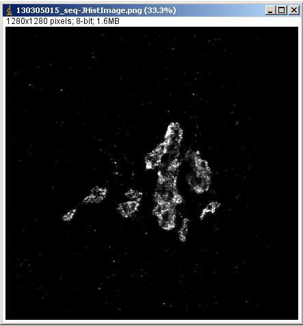
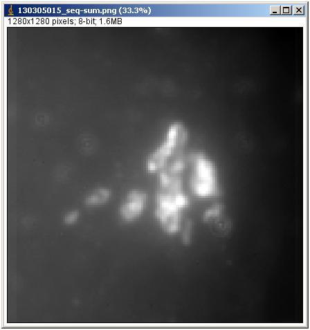
8 Processing a dataset to create a super-resolution image (10) An initial super-resolution image will be generated once the localisation algorithm has completed. This is a preview without any further Quality Control factors than are specified in the main algorithm. (11) A sum (diffraction-limited) image will be generated if selected in the rainstorm GUI (12) Press Open Reviewer and a new GUI will appear

9 Reviewer Quality Control Parameter Definitions Localisations must pass ALL of the following quality control criteria to be accepted into a reviewed image. Updated Signal Counts: This is a minimum brightness threshold. The higher this number the brighter a candidate must be to be accepted as a localistion in the final image. It can be a good way to prevent any dim static background signal from getting into the final super-resolution image. Updated Tolerance: excludes fitted candidates with a high least-squares residual. In practice, it is often best to leave this as a permissive value such as 0.1 (10%). Updated PSF Sigma Range: This is the width of each candidate that is acceptable. Using Alexa 647 or similar with a 160 nm pixel size the theoretical value should be 1.3. Values larger than this can be a result of defocused fluorophores, multiple overlapping fluorophores or spherical aberration. A restrictive range here can remove slightly out of focus molecules, ie. provide some optical sectioning and prevent mislocalisations (the averaging of the positions of 2 or more simultaneously activated fluorophores). Counts Per Photon: This is a calibration value that can be found in the datasheet of the camera. It is dependent on the camera and the gain setting used. Inputting the correct value is required for accurate assessment of precision and resolution. Localisation Precision: This applies a cutoff to reject localisations with a poor localisation precision*. More stringent values (ie. less than 50 nm) will generate images with better mean localisation precisions but with fewer localisations in the final image. *Calculated by the Thompson Formula [Biophys. J. 82(5), (2002) ]. Reconstruction Scale Factor: This determines the size of the pixel in the superresolution image. For example with a pixel width of 160 nm in the raw data a reconstruction scale factor of 5 will generate super-resolution pixels of 32 nm. This is used for the Simple Histogram Visualisation but currently ignored by the Jittered Histogram Visualisation which is able to determine a suitable pixel width for itself. Limit frame range: Can process subsets of the raw data. Often frames early in the sequence can suffer from mislocalisations where the blinking density is too high to fiind single molecules. Later frames may suffer from focus drift.

10 Generating a high quality reviewed super-resolution image (1) Input preliminary review parameters as indicated in the boxes (2) Press Run Reviewer (4) View Histograms (5) Further refine quality control parameters (3) Adjust Contrast (6) Select jittered histogram from Visualisation menu (7) Run Reviewer (8) Adjust contrast (9) Save Image In order for the on screen image and histogram images to be saved the windows must be open and on screen. If the jittered histogram visualisation option is selected then both jitteredhistogram and simple histogram files will be saved. Data gets saved in the same folder as the raw data. Changing any parameters and clicking Save Image again will overwrite previous data.

11 Saved File Types hists info JHistImage onscreenimage STORMdataImage sum

12 Resolution and Image Quality Metrics Candidate brightness: This is related to the number of photons per candidate molecule. If the dye blinking density is high (non-sparse) a large tail or second peak can be seen at higher signal counts. Localisations per Frame: In sparse blinking samples illuminated with constant laser power a gradual decline in accepted localisations will be seen (as above). A sudden drop in localisation number can be a result of focus drift or inappropriate change in illumination conditions, resulting in either many overlapping signals (non-sparse) blinking or no blinking at all. A gradually increasing accepted localisation number tends to indicate a transition from too dense to sparse blinking as more dyes are bleached. Pixel Widths (PSF Sigma): Represents the width of each candidate position in the raw image. Assuming a pixel size of 160 nm and using Alexa 647 or similar this value should be at 1.3. Larger values are indicative of spherical aberration (check the glass thickness, immersion oil and objective lens correction collar), defocus (poor focusing and/or a sample with fluorophores at variable Z positions, or too high blinking densities resulting in mislocalisations). Thompson Localisation Precisions: Is generated from every localisation and is based on the emitted photons (signal counts calibration). A large peak between nm should be seen in good quality datasets. Greyed out regions show data that has been excluded from the reviewed super-resolution image. Large differences in row and column directions are indicative of high density blinking (non-sparse) in samples with orientation such as actin filaments or microtubules. Rees et al. Opt. Nanoscopy 1(1), 12 (2012). Alternative approaches to quantifying resolution are explained by Ram et al, PNAS, 2005, doi pnas and Nieuwenhuizen et al., Nature Methods, 2013, doi: /nmeth.2448

13 Resolution and Image Quality Metrics For more on this see Rees et al, Journal of Optical Nanoscopy, 2012 Precision Limit: This is an estimate of the image resolution based on the signal counts calibrated to photons from the raw data. In this case it is a guide line for the best case ability to discriminate two objects as being separate. If certain parts of the raw images contained high background signal these areas will have worse resolution than indicated. Areas with much higher contrast than the rest of the image will have better resolution. This resolution number does not account for labelling size (in the case of antibody labelling up to 15 nm of distance may be added between fluorophore and molecule of interest). It also does not account for any drift during the image acquisition. Mean Precision Estimate: This is based on the calculated Thompson localisation precisions. Number of accepted localisations: The number of data points in the final image. Being more stringent with quality control criteria will reduce the number of localisations in the final image and can lead to a pointillist (dotty) image. In other words, it has been undersampled. 1 localisation 1 blink. If that blink is spread out across more than one frame it will get localised in each one, i.e. no time-based assessments are made. Overall image quality is dependent on: Structures of interest being well labelled i.e. there is fluorophore attached to most or all of the molecules of interest Accepted localisation number a sufficient number of those labelled molecules have been imaged Mean precision estimate each of those molecules has been imaged well enough to be accurately positioned (a function of photons against background and being in focus) Drift minimal or no movement of the sample in relation to the objective lens throughout the image acquisition Visualisation an appropriate pixel size in simple histogram visualisation method (recommended to use a value the same as the mean precision estimate value). This does not apply when using the jittered histogram method, which is better in most cases than the simple histogram.

14 Comparison of Visualisation methods Simple histogram (10 nm pixels) Simple histogram (25 nm pixels) Simple histogram (40 nm pixels) Simple histogram (25 nm pixels) Jittered histogram In localisation microscopy, a visualisation method is used to convert the localised positions into a reconstructed image of the underlying specimen. Several different visualisation algorithms exist [Baddeley, 2010, Microsc. Microanal ], and the best of these tend to be based on Density Estimation Theory [Silverman, Density Estimation for Statistics and Data Analysis, CRC Press 1985]. A Simple Histogram visualisation reconstructs an image in which the brightness of each of its pixels is proportional to the number of localisations that fall within it. This benefits from simplicity, but requires an optimal choice of pixel size to be made by the user, and also suffers from arbitrary variation due to pixel edge-position. The method of Gaussian Rendering (Baddeley) plots each localisation as a smooth Gaussian bump of density the width of each bump may be optimally scaled (by Adaptive Kernel Density Estimation ) to suit the precision and density of localisations. The Jittered Histogram visualisation [Kricek Opt. Express ] is effectively a digitised form of Gaussian rendering, and in rainstorm the Jittered Histogram visualisation does employ a form of adaptive width smoothing.

15 Box Tracking and Fiduciary Drift Correction : Detecting Drift (1) Process the data review and save images as described (2) Using the zoom tool identify a region of interest with distinctive structure (in this case what looks like a thick actin filament) For more see Metcalf et al, JoVE, 2013 (3) Press Box Tracking & highlight an ROI with the cross hairs on the reviewed image (4) Wait a few seconds and a Boxed Positions image will appear, with localisations colour coded as a function of frame number (ie. time). A displacement of the different colours is an indication that there may be drift present in the image

16 Box Tracking and Fiduciary Drift Correction: Drift Correction For more see Metcalf et al, JoVE, 2013 (1) Process the data review and save images as described (2) Using the zoom tool identify a fiducial marker (3) Press Box Tracking & highlight the bead with cross hairs (4) Wait a few seconds and a Boxed Positions image will appear, with localisations colour-coded as a function of frame number (i.e. time). (5) Press Set Anchor (6) Press Subtract Drift (7) Run Reviewer to generate a new drift corrected image (without the bead included) (8) To remove other beads from the image use box tracking to highlight a bead then press Delete Boxed to remove it. Repeat for additional beads and then run reviewer a final time.

17 Optical Offset Evaluation and Correction (1) Add Tetraspeck beads (or similar) with dyes of appropriate wavelengths using the same type of glass as the sample. (2) Take a single image at each relevant wavelength (with appropriate laser lines and filters) for example 640 nm excitation for a red channel and 561 nm for a green channel (3) Process channel 1 (eg. red), review and save image. (4) Press Capture Ch1 (5) Process channel 2 (eg. green), review and save image. (6) Press Capture Ch2 (7) Press Eval Ch2 offset (8) Capture the red channel from the sample, process, review and save data. (9) Capture the green channel from the sample, process and review. (10) Press Subt Ch2 offset, run reviewer and save data (this channel has now been corrected with respect to Ch1). This chromatic offset correction can be applied to all images acquired at the same wavelengths so long as there are no changes to detection path of the microscope. For more see Erdelyi et al., Optics Express, 2013 Tetraspeck beads before and after Offset Correction Before After

18 Batch Processing Only available in the MATLAB (not compiled) version of rainstorm (1) Process a file, review and save as normal. All subsequent batch processed files will be processed using the same settings as this one. (2) In MATLAB, open file and select rainstorm_extras_batch process.m (3) In the editor window click run and then navigate to a folder containing tif files to be batch processed. Select a file. (4) rainstorm will now process all of the files in that folder. If not parallel processing a waitbar will be displayed for each image. Make sure the computer doesn t go into screen saver or auto-logout modes as the histogram and on screen images will not be properly saved.

19 Particle Tracking Only available in the MATLAB (not compiled) version of rainstorm (1) Process a file, review and save as normal. (2) In MATLAB, open file and select rainstorm_extras_trajectoryfitting.m In development (3) In the editor window click run and trajectory images will be generated

20 3D Astigmatism In development