Microwave Devices & Radar

Transcription

1 Naval Postgraduate School Distance Learning Microwave Devices & Radar LECTURE NOTES VOLUME I by Professor David Jenn Contributors: Professors F. Levien, G. Gill, J. Knorr and J. Lebaric ver4.7

2 Table of Contents (ver4.7) I-1 Table of Contents (1) I-2 Table of Contents (2) I-3 Table of Contents (3) I-4 Table of Contents (4) I-5 Table of Contents (5) I-6 Electromagnetic Fields and Waves (1) I-7 Electromagnetic Fields and Waves (2) I-8 Electromagnetic Fields and Waves (3) I-9 Electromagnetic Fields and Waves (4) I-10 Electromagnetic Fields and Waves (5) I-11 Electromagnetic Fields and Waves (6) I-12 Electromagnetic Fields and Waves (7) I-13 Electromagnetic Fields and Waves (8) I-14 Electromagnetic Fields and Waves (9) I-15 Wave Reflection (1) I-16 Wave Reflection (2) I-17 Wave Reflection (3) I-18 Wave Reflection (4) I-19 Wave Reflection (5) I-20 Wave Reflection (6) I-21 Antenna Patterns, Directivity and Gain I-22 Polarization of Radiation I-23 Wave Polarization I-24 Electromagnetic Spectrum I-25 Radar and ECM Frequency Bands I-26 Radar Bands and Usage I-27 Joint Electronics Type Designation I-28 Examples of EW Systems I-29 Radio Detection and Ranging (RADAR) I-30 Time Delay Ranging I-31 Information Available From the Radar Echo I-32 Radar Classification by Function I-33 Radar Classification by Waveform I-34 Basic Form of the Radar Range Equation (1) I-35 Basic Form of the Radar Range Equation (2) I-36 Basic Form of the Radar Range Equation (3) I-37 Characteristics of the Radar Range Equation I-38 Maximum Detection Range I-39 Generic Radar Block Diagram I-40 Brief Description of System Components I-41 Coordinate Systems I-42 Radar Displays I-43 Pulsed Waveform I-44 Range Ambiguities I-45 Range Gates I-46 Range Bins and Range Resolution I-47 Radar Operational Environment I-48 Ground Clutter From Sidelobes I-49 Survey of Propagation Mechanisms (1) I-50 Survey of Propagation Mechanisms (2) I-51 Survey of Propagation Mechanisms (3) I-52 Radar System Design Tradeoffs I-53 Decibel Refresher I-54 Thermal Noise I-55 Noise in Radar Systems I-56 Noise in Radar Systems I-57 Ideal Filter I-58 Noise Bandwidth of an Arbitrary Filter I-59 Signal-to-noise Ratio (S/N) I-60 Example: Police Radar I-61 Attack Approach I-62 Defeating Radar by Jamming 1 I-63 Jammer Burnthrough Range (1) I-64 Jammer Burnthrough Range (2) I-65 Noise Figure I-66 Probability & Statistics Refresher (1) I-67 Probability & Statistics Refresher (2) I-68 Probability & Statistics Refresher (3) I-69 Probability & Statistics Refresher (4) I-70 Rayleigh Distribution (1) I-71 Rayleigh Distribution (2) I-72 Central Limit Theorem I-73 Transformation of Variables I-74 Fourier Transform Refresher (1) I-75 Fourier Transform Refresher (2) I-76 Fourier Transform Refresher (3) I-77 Fourier Transform Refresher (4) I-78 Fourier Transform Refresher (5) I-79 Modulation of a Carrier (1) I-80 Modulation of a Carrier (2) I-81 Modulation of a Carrier (3) I-82 Fourier Transform of a Pulse Train (1) I-83 Fourier Transform of a Pulse Train (2) I-84 Fourier Transform of a Pulse Train (3) I-85 Response of Networks (1) I-86 Response of Networks (2) I-87 Response of Networks (3) I-88 Signals and Noise Through Networks (1) I-89 Signals and Noise Through Networks (2) I-90 Signals and Noise Through Networks (3) I-91 Rician Distribution I-92 Probability of False Alarm (1) I-93 Probability of False Alarm (2) I-94 Probability of False Alarm (3) I-95 Probability of Detection (1) I-96 Probability of Detection (2) I-97 Probability of Detection (3) I-98 Probability of Detection I-99 SNR Improvement Using Integration I-100 Illustration of Coherent Integration I-101 SNR Improvement Using Integration I-102 Approximate Antenna Model I-103 Number of Pulses Available I-104 Integration Improvement Factor I-105 RRE for Pulse Integration I-106 RRE for Pulse Integration I-107 RRE for Pulse Integration I-108 Radar Cross Section (1) I-109 Radar Cross Section (2) I-110 Radar Cross Section of a Sphere I-111 Radar Cross Section of a Cylinder I-112 Target Scattering Matrix (1) I-113 Target Scattering Matrix (2) I-114 Example: Antenna as a Radar Target I-115 Scattering Mechanisms I-116 Scattering Sources for a Complex Target I-117 Two Sphere RCS (1) I-118 Two Sphere RCS (2) I-119 RCS of a Two Engine Bomber I-120 RCS of a Naval Auxiliary Ship I-121 RCS of a Geometrical Components Jet I-122 Geometrical Components Jet I-123 Fluctuating Targets I-124 Swerling Types

3 I-125 Correction & Improvement Factors (1) I-126 Correction & Improvement Factors (2) I-127 Detection Range for Fluctuating Targets I-128 Example I-129 Defeating Radar by Low Observability I-130 Methods of RCS Reduction and Control I-131 Reduction by Shaping: Corner Reflector I-132 Application of Serrations to Reduce Edge Scattering I-133 Application of Serrations to Reduce Edge Scattering I-134 Traveling Waves I-135 Trailing Edge Resistive Strips I-136 Application of Reduction Methods I-137 Low Observable Platforms: F-117 I-138 Low Observable Platforms: B-2 I-139 Low Observable Platforms: Sea Shadow II-1 Other Sources of Loss II-2 Atmospheric Attenuation II-3 Rain Attenuation II-4 Transmission Line Loss II-5 Antenna Beamshape Loss II-6 Collapsing Loss II-7 Noise Figure & Effective Temperature (1) II-8 Comments on Noise Figure & Temperature II-9 Noise in Cascaded Networks (1) II-10 Noise Figure & Effective Temperature (2) II-11 Noise Figure From Loss II-12 Examples (1) II-13 Examples (2) II-14 Examples (3) II-15 Examples (4) II-16 Examples (5) II-17 Examples (6) II-18 Examples (7) II-19 Doppler Frequency Shift (1) II-20 Doppler Frequency Shift (2) II-21 Doppler Frequency Shift (3) II-22 Doppler Filter Banks II-23 Example II-24 Example II-25 I and Q Representation II-26 Doppler Frequency Shift (4) II-27 CW Radar Problems (1) II-28 CW Radar Problems (2) II-29 CW Radar Problems (3) II-30 Frequency Modulated CW (FMCW) II-31 FMCW (2) II-32 FMCW (3) II-33 FMCW (4) II-34 FMCW Complications II-35 FMCW Complications II-36 MTI and Pulse Doppler Radar II-37 MTI (1) II-38 MTI (2) II-39 MTI (3) II-40 PD and MTI Problem: Eclipsing II-41 PD and MTI Problem: Range Ambiguities II-42 Range Ambiguities (2) II-43 Range Ambiguities (3) II-44 Example II-45 PD and MTI Problem: Velocity Ambiguities II-46 Velocity Ambiguities (2) II-47 II-48 Surface Clutter (1) II-49 Surface Clutter (2) Airborne MTI and Pulse Doppler Operation II-50 Surface Clutter (3) II-51 Two-Way Pattern Beamwidth II-52 Surface Clutter (4) II-53 Backscatter From Extended Surfaces II-54 Backscatter From Extended Surfaces II-55 Clutter Spectrum (1) II-56 Clutter Spectrum (2) II-57 Clutter Spectrum (3) II-58 Clutter Spectrum (4) II-59 Clutter Spectrum (5) II-60 Clutter Spectrum (6) II-61 Clutter Spectrum (7) II-62 Sea States II-63 Sea Clutter II-64 Example: AN/APS-200 II-65 Example: AN/APS-200 II-66 Example: AN/APS-200 II-67 Delay Line Canceler (1) II-68 Delay Line Canceler (2) II-69 Delay Line Canceler (3) II-70 Delay Line Canceler (4) II-71 Staggered and Multiple PRFs (1) II-72 Staggered and Multiple PRFs (2) II-73 Staggered and Multiple PRFs (3) II-74 Synchronous Detection (I and Q Channels) II-75 Analog vs Digital Processing for MTI II-76 Single Channel Receiver Block Diagram II-77 Synchronous Receiver Block Diagram II-78 SNR Advantage of Synchronous Detection (1) II-79 SNR Advantage of Synchronous Detection (2) II-80 Processing of a Coherent Pulse Train (1) II-81 Sampling Theorem (1) II-82 Sampling Theorem (2) II-83 Processing of a Coherent Pulse Train (2) II-84 Processing of a Coherent Pulse Train (3) II-85 Processing of a Coherent Pulse Train (4) II-86 Discrete Fourier Transform (DFT) II-87 Doppler Filtering Using the DFT (1) II-88 Doppler Filtering Using the DFT (2) II-89 Pulse Doppler Receiver II-90 Pulse Burst Mode II-91 MTI Improvement Factors II-92 MTI Limitations (1) II-93 MTI Limitations (2) II-94 MTI Canceler Improvement Factors II-95 MTI Canceler Improvement Factors II-96 Example II-97 Coherent and Noncoherent Pulse Trains II-98 Noncoherent Pulse Train Spectrum (1) II-99 Noncoherent Pulse Train Spectrum (2) II-100 Search Radar Equation (1) II-101 Search Radar Equation (2) II-102 Search Radar Equation (3) II-103 Search Radar Equation (4) II-104 Radar Tracking (1) II-105 Radar Tracking (2) II-106 Radar Tracking (3) II-107 Gain Control II-108 Example II-109 Example II-110 Monopulse Tracking (1) II-111 Monopulse Tracking (2) II-112 Monopulse Tracking (3) II-113 Monopulse Tracking (4) II-114 Monopulse Tracking (5) II-115 Monopulse Tracking (6) II-116 Monopulse Tracking (7) II-117 Low Angle Tracking (1) 2

4 II-118 Low Angle Tracking (2) II-119 Low Angle Tracking (3) II-120 Low Angle Tracking (4) II-121 Tracking Error Due to Multipath II-122 Low Angle Tracking (5) II-123 Low Angle Tracking (6) II-124 Atmospheric Refraction (1) II-125 Atmospheric Refraction (2) II-126 Atmospheric Refraction (3) III-1 Receiver Types (1) III-2 Receiver Types (2) III-3 Noise Power Spectral Density III-4 Matched Filters (1) III-5 Matched Filters (2) III-6 Matched Filters (3) III-7 Matched Filters (4) III-8 Matched Filters (5) III-9 Matched Filters (6) III-10 Matched Filters (7) III-11 Complex Signals III-12 Ambiguity Function (1) III-13 Ambiguity Function (2) III-14 Ambiguity Function (3) III-15 Ambiguity Function (4) III-16 Ambiguity Function (5) III-17 Range Accuracy (1) III-18 Range Accuracy (2) III-19 Range Accuracy (3) III-20 Range Accuracy (4) III-21 Velocity Accuracy III-22 Uncertainty Relation III-23 Angular Accuracy III-24 Pulse Compression III-25 Linear FM Pulse Compression (Chirp) III-26 Linear FM Pulse Compression (Chirp) III-27 Linear FM Pulse Compression (Chirp) III-28 Linear FM Pulse Compression (Chirp) III-29 Chirp Filter Output Waveform III-30 Range Resolution (1) III-31 Range Resolution (2) III-32 Pulse Compression Example III-33 Chirp Complications III-34 Digital Pulse Compression III-35 Barker Sequences III-36 Pulse Compessor/Expander III-37 The Ideal Radar Antenna III-38 Antenna Refresher (1) III-39 Lens Antenna III-40 Solid Angles and Steradians III-41 Antenna Far Field III-42 Antenna Pattern Features III-43 Antenna Refresher (2) III-44 Antenna Refresher (3) III-45 Directivity Example III-46 Antenna Polarization Loss III-47 Parabolic Reflector Antenna III-48 Parabolic Reflector Antenna Losses III-49 Example III-50 Example III-51 Radiation by a Line Source (1) III-52 Radiation by a Line Source (2) III-53 Array Antennas (1) III-54 Array Antennas (2) III-55 Visible Region III-56 Array Antennas (3) III-57 Array Antennas (4) III-58 Array Factor for 2D Arrays III-59 Gain of Phased Arrays III-60 Array Elements and Ground Planes III-61 Array of Dipoles Above a Ground Plane III-62 Series Fed Waveguide Slot Array III-63 Low Probability of Intercept Radar (LPIR) III-64 Low and Ultra Low Sidelobes III-65 Antenna Pattern Control III-66 Tapered Aperture Distributions III-67 Calculation of Aperture Efficiency III-68 Cosecant-Squared Antenna Pattern III-69 Example III-70 Array Example (1) III-71 Array Example (2) III-72 Array Example (3) III-73 Array Example (4) III-74 Calculation of Antenna Temperature III-75 Multiple Beam Antennas (1) III-76 Multiple Beam Antennas (2) III-77 Radiation Patterns of a Multiple Beam Array III-78 Beam Coupling Losses for a 20 Element Array III-79 Active vs Passive Antennas III-80 SNR Calculation for a Lossless Feed Network III-81 SNR Calculation for a Lossless Feed Network III-82 Passive Two-Beam Array (1) III-83 Passive Two-Beam Array (2) III-84 Active Two-Beam Array (1) III-85 Active Two-Beam Array (2) III-86 Comparison of SNR: Active vs Passive III-87 Example III-88 Active Array Radar Transmit/Receive Module III-89 Digital Phase Shifters III-90 Effect of Phase Shifter Roundoff Errors III-91 Digital Phase Shifters III-92 True Time Delay Scanning III-93 Time Delay vs Fixed Phase Scanning III-94 Beam Squint Due to Frequency Change III-95 Time Delay Networks III-96 Time Delay Using Fiber Optics III-97 Digital Beamforming (1) III-98 Digital Beamforming (2) III-99 Monopulse Difference Beams III-100 Sum and Difference Beamforming III-101 Waveguide Monopulse Beamforming Network III-102 Antenna Radomes III-103 Conformal Antennas & "Smart Skins" III-104 Testing of Charred Space Shuttle Tile III-105 Antenna Imperfections (Errors) III-106 Smart Antennas (1) III-107 Smart Antennas (2) III-108 Microwave Devices III-109 Transmission Line Refresher (1) III-110 Transmission Line Refresher (2) III-111 Transmission Line Refresher (3) III-112 Multiplexers III-113 Rotary Joints III-114 Microwave Switches III-115 Circulators III-116 Waveguide Magic Tee III-117 Filter Characteristics III-118 Mixers (1) III-119 Mixers (2) III-120 Mixers (3) III-121 Input-Output Transfer Characteristic III-122 Intermodulation Products III-123 Intermodulation Example 3

5 III-124 Amplifiers III-125 Low-Noise Amplifier III-126 Intermodulation Products of Amplifiers III-127 Sample Microwave Amplifier Characteristic III-128 Power Capabilities of Sources III-129 Development of Sources III-130 Transmitters (1) III-131 Transmitters (2) III-132 Klystrons III-133 Klystron Operation III-134 Cavity Magnetron III-135 Magnetron Operation III-136 Eight Cavity Magnetron III-137 Magnetron Basics (1) III-138 Magnetron Basics (2) III-139 Free-Electron Laser (FEL) Operation III-140 Free-Electron Lasers III-141 Radar Waveform Parameter Measurements (1) III-142 Radar Waveform Parameter Measurements (2) III-143 Radar Waveform Parameter Measurements (3) III-144 Radar Waveform Parameter Measurements (4) III-145 Radar Waveform Parameter Measurements (5) IV-1 Special Radar Systems and Applications IV-2 AN/TPQ-37 Firefinder Radar IV-3 Firefinder Radar Antenna (1) IV-4 Firefinder Radar Antenna (2) IV-5 AN/TPQ-37 Subarray IV-6 Firefinder Radar Antenna (3) IV-7 Patriot Air Defense Radar (1) IV-8 Patriot Air Defense Radar (2) IV-9 SCR-270 Air Search Radar IV-10 SCR-270-D Radar IV-11 SPY-1 Shipboard Radar IV-12 X-Band Search Radar (AN/SPS-64) IV-13 AN/SPS-64 IV-14 C-Band Search Radar (AN/SPS-67) IV-15 AN/SPS-67 IV-16 Combat Surveillance Radar (AN/PPS-6) IV-17 AN/PPS-6 IV-18 Early Air Surveillance Radar (AN/APS-31) IV-19 AN/APS-31 IV-20 AN/APS-40 IV-21 AN/APS-40 IV-22 Plan Position Indicator (PPI) IV-23 Radiometers (1) IV-24 Radiometers (2) IV-25 Radiometers (3) IV-26 Radiometers (4) IV-27 Radiometers (5) IV-28 Harmonic Radar (1) IV-29 Harmonic Radar (2) IV-30 Harmonic Radar Tracking of Bees IV-31 Synthetic Aperture Radar (SAR) IV-32 SAR (2) IV-33 SAR (3) IV-34 Comparison of Array Factors IV-35 Image Resolution IV-36 Unfocused SAR (1) IV-37 Unfocused SAR (2) IV-38 Focused SAR IV-39 Example IV-40 Cross Range Processing (1) IV-41 Cross Range Processing (2) IV-42 Cross Range Processing (3) IV-43 Motion Compensation IV-44 Radar Mapping IV-45 SAR Image IV-46 SAR Range Equation IV-47 SAR Problems (1) IV-48 SAR Problems (2) IV-49 Inverse Synthetic Aperture Radar (ISAR) IV-50 ISAR (2) IV-51 ISAR (3) IV-52 ISAR (4) IV-53 HF Radars (1) IV-54 HF Radars (2) IV-55 HF Radars (3) IV-56 Typical HF OTH Radar Parameters IV-57 Typical HF Clutter and Target Spectrum IV-58 Relocatable OTH Radar (ROTHR) IV-59 HF Coastal Radar (CODAR) IV-60 HF Radar Example (CONUS-B) IV-61 Stepped Frequency Radar (1) IV-62 Stepped Frequency Radar (2) IV-63 Stepped Frequency Radar (3) IV-64 Stepped Frequency Radar (4) IV-65 Stepped Frequency Radar (5) IV-66 Stepped Frequency Radar (6) IV-67 Imaging of Moving Targets IV-68 Stepped Frequency Imaging (1) IV-69 Stepped Frequency Imaging (2) IV-70 Stepped Frequency Imaging (3) IV-71 Ultra-Wide Band Radar (1) IV-72 Ultra-Wide Band Radar (2) IV-73 Ultra-Wide Band Radar (3) IV-74 Ultra-Wide Band Radar (4) IV-75 Ultra-Wide Band Radar (5) IV-76 Ultra-Wide Band Radar (6) IV-77 Ultra-Wide Band Radar (7) IV-78 Ultra-Wide Band Radar (8) IV-79 RCS Considerations IV-80 Time Domain Scattering IV-81 F-111 Resonant Frequencies IV-82 Currents on a F-111 at its First Resonance IV-83 Excitation of the First Resonance IV-84 Antenna Considerations IV-85 Brown Bat Ultrasonic Radar (1) IV-86 Brown Bat Ultrasonic Radar (2) IV-87 Doppler Weather Radar (1) IV-88 Doppler Weather Radar (2) IV-89 Doppler Weather Radar (3) IV-90 Doppler Weather Radar (4) IV-91 Doppler Weather Radar (5) IV-92 Implementation and Interpretation of Data (1) IV-93 Implementation and Interpretation of Data (2) IV-94 Implementation and Interpretation of Data (3) IV-95 Implementation and Interpretation of Data (4) IV-96 Implementation and Interpretation of Data (5) IV-97 Clear Air Echoes and Bragg Scattering IV-98 Weather Radar Example IV-99 Monolithic Microwave Integrated Circuits IV-100 Tile Concept IV-101 Module Concept IV-102 MMIC Single Chip Radar (1) IV-103 MMIC Single Chip Radar (2) IV-104 MMIC FMCW Single Chip Radar (1) IV-105 MMIC FMCW Single Chip Radar (2) IV-106 Defeating Radar Using Chaff IV-107 Chaff (1) IV-108 Chaff (2) IV-109 Chaff (3) IV-110 Chaff and Flares 4

6 IV-111 Bistatic Radar (1) IV-112 Bistatic Radar (2) IV-113 Flight-Tracking Firm Takes Off IV-114 Bistatic Radar (3) IV-115 Bistatic Radar (4) IV-116 Bistatic Radar Example (1) IV-117 Bistatic Radar (5) IV-118 Bistatic Radar (6) IV-119 Bistatic Radar (7) IV-120 Bistatic Radar (8) IV-121 Bistatic Radar (9) IV-122 Bistatic Radar (10) IV-123 Bistatic Radar Example (2) IV-124 Line-of-Sight Constrained Coverage (1) IV-125 Line-of-Sight Constrained Coverage (2) IV-126 Bistatic Radar (11) IV-127 Bistatic Radar (12) IV-128 Bistatic Footprint and Clutter Area (1) IV-129 Bistatic Footprint and Clutter Area (2) IV-130 Bistatic Radar Cross Section (1) IV-131 Bistatic Radar Cross Section (2) IV-132 Bistatic Radar Example Revisited IV-133 Bistatic Radar Cross Section (3) IV-134 Cross Eye Jamming (1) IV-135 Cross Eye Jamming (2) IV-136 ECM for Conical Scanning IV-137 Ground Bounce ECM IV-138 Suppression of Sidelobe Jammers (1) IV-139 Suppression of Sidelobe Jammers (2) IV-140 CSLC Equations for an Array Antenna IV-141 CSLC Performance IV-142 Adaptive Antennas IV-143 Laser Radar (1) IV-144 Laser Radar (2) IV-145 Laser Radar (3) IV-146 Laser Radar (4) IV-147 Laser Radar (5) IV-148 Laser Radar (6) IV-149 Laser Radar (7) IV-150 Laser Radar (8) IV-151 Ground Penetrating Radar (1) IV-152 Ground Penetrating Radar (2) IV-153 Ground Penetrating Radar (3) IV-154 Ground Penetrating Radar (4) IV-155 Ground Penetrating Radar (5) IV-156 Ground Penetrating Radar (6) IV-157 Ground Penetrating Radar (7) IV-158 Ground Penetrating Radar (8) 5

7 Electromagnetic Fields and Waves (1) Radar is based on the sensing of electromagnetic waves reflected from objects. Energy is emitted from a source (antenna) and propagates outward. A point on the wave travels with a phase velocity u p, which depends on the electronic properties of the medium in which the wave is propagating. From antenna theory: if the observer is sufficiently far from the source, then the surfaces of constant phase (wavefronts) are spherical. At even larger distances the wavefronts become approximately planar. SPHERICAL WAVE FRONTS PLANE WAVE FRONTS RAYS 6

8 Electromagnetic Fields and Waves (2) Snapshot of a spherical wave propagating outward from the origin. The amplitude of the wave E ( R,t) = θ ˆ E o cos(ωt βr) in the x-y plane is plotted at time t = 0 R 7

9 Electromagnetic Fields and Waves (3) Snapshot of a plane wave propagating in the + y direction E (y,t) = z ˆ E o cos(ωt βy) at time t = 0 8

10 Electromagnetic Fields and Waves (4) Electrical properties of a medium are specified by its constitutive parameters: permeability, µ = µ o µ r (for free space, µ µ o = 4π 10 7 H/m) permittivity, ε = ε o ε r (for free space, ε ε o = F/m) conductivity, σ (for a metal, σ ~ 10 7 S/m) Electric and magnetic field intensities: E ( x, y, z,t) V/m and H (x, y,z,t) A/m vector functions of location in space and time, e.g., in cartesian coordinates E (x,y,z,t) = x ˆ E x (x,y,z,t) + y ˆ E y (x,y,z,t) + z ˆ E z (x,y,z,t) similar expressions for other coordinates systems the fields arise from current J and charge ρ v on the source ( J is the volume current density in A/m 2 and ρ v is volume charge density in C/m 3 ) Electromagnetic fields are completely described by Maxwell s equations: (1) E = µ H (3) H = 0 t (2) H = J + ε E t (4) E = ρ v / ε 9

11 Electromagnetic Fields and Waves (5) The wave equations are derived from Maxwell s equations: 2 E 1 2 E 2 u p t 2 = 0 2 H 1 2 H 2 u p t 2 = 0 The phase velocity is u p = ω µ ε (in free space u p = c = m/s) The simplest solutions to the wave equations are plane waves. An example for a plane wave propagating in the z direction is: E (z,t) = x ˆ E o e αz cos(ω t βz) α = attenuation constant (Np/m); β = 2π / λ = phase constant (rad/m) λ = wavelength; ω = 2π f (rad/sec); f = frequency (Hz); f = u p λ Features of this plane wave: propagating in the + z direction x polarized (direction of electric field vector is x ˆ ) amplitude of the wave is E o 10

12 Electromagnetic Fields and Waves (6) Time-harmonic sources, currents, and fields: sinusoidal variation in time and space. Suppress the time dependence for convenience and work with time independent quantities called phasors. A time-harmonic plane wave is represented by the phasor E (z) ( α + { j β ) o z j ω E z t xe e e t } { E z e j ω (, ) = Re ˆ = Re ( ) t } E (z) is the phasor representation; E ( z, t) is the instantaneous quantity Re {} is the real operator (i.e., take the real part of ) j = 1 Since the time dependence varies as e jω t, the time derivatives in Maxwell s equations are replaced by / t jω : (1) E = jωµ H (3) H = 0 (2) H = J + jωε E (4) E = ρ v /ε The wave equations are derived from Maxwell s equations: 2 E γ 2 E = 0 2 H γ 2 H = 0 where γ = α + jβ is the propagation constant. 11

13 Electromagnetic Fields and Waves (7) Plane and spherical waves belong to the to a class called transverse electromagnetic (TEM) waves. They have the following features: 1. E, H and the direction of propagation k ˆ are mutually orthogonal 2. E and H are related by the intrinsic impedance of the medium η = µ (ε jσ /ω ) η o = µ o ε o 377 Ω for free space The above relationships are expressed in the vector equation H k = ˆ E η The time-averaged power propagating in the plane wave is given by the Poynting vector: W E o 2 For a plane wave: W (z) = 1 2 η For a spherical wave: W (R) = 1 2η { E H * } 1 = Re W/m 2 2 ˆ z E o 2 R 2 ˆ R (inverse square law for power spreading) 12

14 Electromagnetic Fields and Waves (8) A material s conductivity causes attenuation of a wave as it propagates through the medium. Energy is extracted from the wave and dissipated as heat (ohmic loss). The attenuation constant determines the rate of decay of the wave. In general: 1/ 2 1/ σ µε 1 1 σ + β = ω ωε 2 ωε µε α = ω For lossless media σ = 0 α = 0. Traditionally, for lossless cases, k is used rather than β. For good conductors (σ /ωε >> 1), α π µ fσ, and the wave decays rapidly with distance into the material. 1 Sample plot of field vs. distance ELECTRIC FIELD STRENGTH (V/m) DEPTH INTO MATERIAL (m) 13

15 Electromagnetic Fields and Waves (9) For good conductors the current is concentrated near the surface. The current can be approximated by an infinitely thin current sheet, or surface current, J s A/m and surface charge, ρ s C/m Current in a good conductor ˆ k i J E i BOUNDARY Surface current approximation ˆ k i J s E i BOUNDARY At an interface between two media the boundary conditions must be satisfied: (1) n ˆ 21 ( E 1 E 2 ) = 0 (2) n ˆ 21 ( H 1 H 2 ) = J s REGION 1 REGION 2 ˆ n 21 (3) n ˆ 21 ( E 1 E 2 ) = ρ s /ε (4) n ˆ 21 ( H 1 H 2 ) = 0 J s ρ s INTERFACE 14

16 Wave Reflection (1) For the purposes of applying boundary conditions, the electric field vector is decomposed into parallel and perpendicular components E = E + E E is perpendicular to the plane of incidence E lies in the plane of incidence The plane of incidence is defined by the vectors k ˆ i and n ˆ PLANE WAVE INCIDENT ON AN INTERFACE BETWEEN TWO DIELECTRICS MEDIUM 2 MEDIUM 1 θ i NORMAL TRANSMITTED θ t θ r ε 2,µ 2 ε 1,µ 1 DECOMPOSITON OF AN ELECTRIC FIELD VECTOR INTO PARALLEL AND PERPENDICULAR COMPONENTS INTERFACE z ˆ n θ i ˆ k i E E E y INCIDENT REFLECTED x 15

17 Wave Reflection (2) Plane wave incident on an interface between free space and a dielectric REGION 1 REGION 2 FREE SPACE ε o µ o ˆ n ˆ k r η o = θ i θ r ˆ k i sin θ i = sin θ r = µ o ε o and η = DIELECTRIC ε r µ r θ t INTERFACE ε r µ r sin θ t µ r µ o ε r ε o = η o µ r ε r Reflection and transmission coefficients: Perpendicular polarization: Γ = ηcosθ i η 0 cosθ t ηcosθ i + η 0 cosθ t 2ηcosθ τ = i ηcosθ i +η 0 cosθ t E r = Γ E i and E t = τ E i Parallel polarization: Γ = ηcosθ t η 0 cosθ i ηcosθ t +η 0 cosθ i 2ηcosθ τ = i ηcosθ t + η 0 cosθ i E r = Γ E i and E t = τ E i 16

18 Wave Reflection (3) Example of a plane wave incident on a boundary between air and glass (ε r = 4, θ i = 45 ) 10 INCIDENT WAVE TRANSMITTED 8 6 GLASS θ t 4 z 2 0 BOUNDARY AIR θ i θ r -2 NORMAL -4-6 INCIDENT REFLECTED x 17

19 Wave Reflection (4) Example of a plane wave reflection: reflected and transmitted waves (ε r = 4, θ i = 45 ) 10 REFLECTED WAVE 10 TRANSMITTED WAVE z BOUNDARY z BOUNDARY x x 18

20 Wave Reflection (5) Example of a plane wave reflection: total field 10 8 The total field in region 1 is the sum of the incident and reflected fields 6 z BOUNDARY If region 2 is more dense than region 1 (i.e., ε r2 > ε r1 ) the transmitted wave is refracted towards the normal If region 1 is more dense than region 2 (i.e., ε r1 > ε r2 ) the transmitted wave is refracted away from the normal x 19

21 Wave Reflection (6) Boundary between air (ε r = 1) and glass (ε r = 4) AIR-GLASS INTERFACE,WAVE INCIDENT FROM AIR AIR-GLASS INTERFACE,WAVE INCIDENT FROM GLASS PERPENDICULAR POLARIZATION PERPENDICULAR POLARIZATION gamma PARALLEL POLARIZATION BREWSTER'S ANGLE gamma PARALLEL POLARIZATION theta, degrees theta, degrees 20

22 Antenna Patterns, Directivity and Gain The antenna pattern is a directional plot of the received or transmitted) signal From a systems point of view, two important antenna parameters are gain and beamwidth Both gain and beamwidth are measures of the antenna s capability to focus radiation Gain includes loss that occurs within the antenna whereas directivity refers to a lossless antenna of the same type (i.e., it is an ideal reference) In general, an increase in gain is accompanied by a decrease in beamwidth, and is achieved by increasing the antenna size relative to the wavelength With regard to radar, high gain an narrow beams are desirable for long detection and tracking ranges and accurate direction measurement LOW GAIN HIGH GAIN ANTENNA DIRECTIONAL RADIATION PATTERN 21

23 Polarization of Radiation Example of a plane wave generated by a linearly polarized antenna: 1. Finite sources generate spherical waves, but they are locally planar over limited regions of space 2. Envelopes of the electric and magnetic field vectors are plotted 3. E and H are orthogonal to each other and the direction of propagation. Their magnitudes are related by the intrinsic impedance of the medium (i.e., TEM) 4. Polarization refers to the curve that the tip of E traces out with time at a fixed point in space. It is determined by the antenna geometry and its orientation relative to the observer E λ kˆ H PROPAGATION DIRECTION ANTENNA 22

24 Wave Polarization LINEAR POLARIZATION 1 2 PARTIALLY POLARIZED CIRCULAR POLARIZATION UNPOLARIZED (RANDOM POLARIZATION) 3 4 ELLIPTICAL POLARIZATION ELECTRIC FIELD VECTOR AT AN INSTANT IN TIME

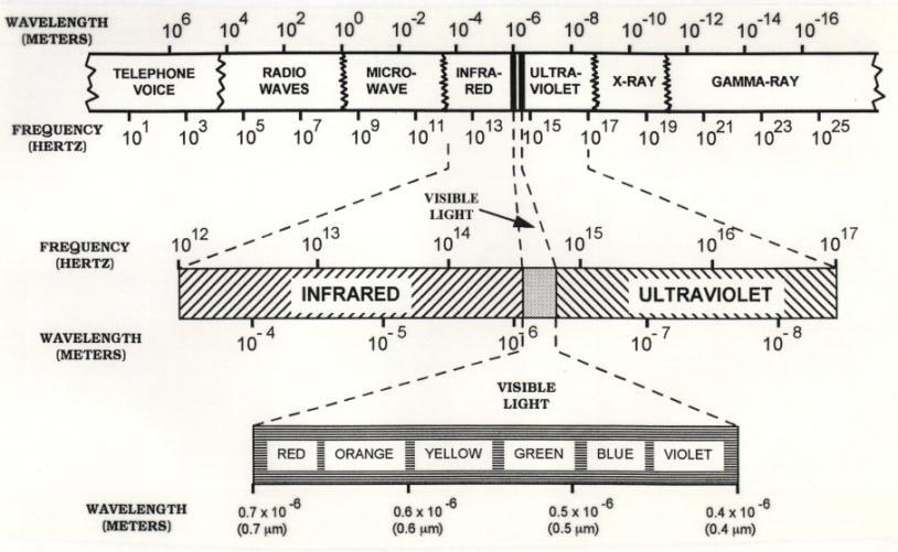
25 Electromagnetic Spectrum 24

26 Radar and ECM Frequency Bands 25

27 Radar Bands and Usage 8 26

28 Joint Electronics Type Designation 27

29 Examples of EW Systems 28

30 Radio Detection and Ranging (RADAR) RECEIVER (RX) TRANSMITTER (TX) R r SCATTERED WAVE FRONTS R t θ TARGET INCIDENT WAVE FRONTS Bistatic: the transmit and receive antennas are at different locations as viewed from the target (e.g., ground transmitter and airborne receiver, θ 0) Monostatic: the transmitter and receiver are colocated as viewed from the target (i.e., the same antenna is used to transmit and receiver, θ = 0) Quasi-monostatic: the transmit and receive antennas are slightly separated but still appear to be at the same location as viewed from the target (e.g., separate transmit and receive antennas on the same aircraft, θ 0) 29

31 Time Delay Ranging Target range is the fundamental quantity measured by most radars. It is obtained by recording the round trip travel time of a pulse, T R, and computing range from: bistatic: R t + R r = ct R monostatic: R = ct R 2 (R r = R t R) where c m/s is the velocity of light in free space. AMPLITUDE TRANSMITTED PULSE RECEIVED PULSE T R TIME 30

32 Information Available From the Radar Echo "Normal" radar functions: 1. range (from pulse delay) 2. velocity (from doppler frequency shift) 3. angular direction (from antenna pointing) 4. target size (from magnitude of return) Signature analysis and inverse scattering: 5. target shape and components (return as a function of direction) 6. moving parts (modulation of the return) 7. material composition The complexity (cost & size) of the radar increases with the extent of the functions that the radar performs. 31

33 Radar Classification by Function Radars Civilian Weather Avoidance Navagation & Tracking Search & Surveillance High Resolution Imaging & Mapping Military Space Flight Sounding Proximity Fuzes Countermeasures Many modern radars perform multiple functions ("multi-function radar") 32

34 Radar Classification by Waveform Radars CW Pulsed FMCW Noncoherent Coherent Low PRF Note: CW = continuous wave FMCW = frequency modulated continuous wave PRF = pulse repetition frequency Medium High PRF PRF ("Pulse doppler") 33

35 Basic Form of the Radar Range Equation (1) Quasi-monostatic geometry TX P t G t R RX P r G r σ σ = radar cross section (RCS) in square meters P t = transmitter power, watts P r = received power, watts G t = transmit antenna gain in the direction of the target (assumed to be the maximum) G r = receive antenna gain in the direction of the target (assumed to be the maximum) P t G t = effective radiated power (ERP) From antenna theory: G r = 4πA er λ 2 A er = A p ρ = effective area of the receive antenna A p = physical aperture area of the antenna λ = wavelength (= c / f ) ρ = antenna efficiency 34

36 Basic Form of the Radar Range Equation (2) Power density incident on the target P t G t R POWER DENSITY AT RANGE R W i = P t G t 4πR 2 (W / m 2 ) Power collected by the radar target INCIDENT WAVE FRONT IS APPROXIMATELY PLANAR AT THE TARGET TARGET EFFECTIVE COLLECTION AREA IS σ P c = σw i = P t G t σ 4πR 2 35

37 Basic Form of the Radar Range Equation (3) The RCS gives the fraction of incident power that is scattered back toward the radar. Therefore, P s = P c and the scattered power density at the radar is obtained by dividing by 4πR 2. RECEIVER (RX) SCATTERED POWER DENSITY AT RANGE R FROM THE TARGET W s = P s TARGET RCS σ 4πR 2 The target scattered power collected by the receiving antenna is W s A er. Thus the maximum target scattered power that is available to the radar is P r = P t G t σa er (4πR 2 ) 2 = P t G t G r σλ2 (4π) 3 R 4 This is the classic form of the radar range equation (RRE). 36

38 Characteristics of the Radar Range Equation P r = P t G t σa er (4πR 2 ) 2 = P t G t G r σλ2 (4π) 3 R 4 For monostatic systems a single antenna is generally used to transmit and receive so that G t = G r G. This form of the RRE is too crude to use as a design tool. Factors have been neglected that have a significant impact on radar performance: noise, system losses, propagation behavior, clutter, waveform limitations, etc. We will discuss most of these in depth later in the course. This form of the RRE does give some insight into the tradeoffs involved in radar design. The dominant feature of the RRE is the 1/ R 4 factor. Even for targets with relatively large RCS, high transmit powers must be used to overcome the 1/ R 4 when the range becomes large. 37

39 Maximum Detection Range The minimum received power that the radar receiver can "sense" is referred to a the minimum detectable signal (MDS) and is denoted S min. P r P r 1 / R 4 S min R max R Given the MDS, the maximum detection range can be obtained: P r = S min = P t G t G r σλ2 (4π) 3 R 4 R max = P t G t G r σλ2 (4π) 3 S min 1 / 4 38

40 Generic Radar Block Diagram This receiver is a superheterodyne receiver because of the intermediate frequency (IF) amplifier. 39

41 Brief Description of System Components DUPLEXER TRANSMITTER LOW NOISE AMPLIFIER (LNA) MIXER MATCHED FILTER IF AMPLIFIER DETECTOR VIDEO AMPLIFIER DISPLAY An antenna switch that allows the transmit and receive channels to share the antenna. Often it is a circulator. The duplexer must effectively isolate the transmit and receive channels. Generates and amplifies the microwave signal. Amplifies the weak received target echo without significantly increasing the noise level. Mixing (or heterodyning) is used to translate a signal to a higher frequency Extracts the signal from the noise Further amplifies the intermediate frequency signal Translates the signal from IF to baseband (zero frequency) Amplifies the baseband signal Visually presents the radar signal for interpretation by the operator 40

42 Coordinate Systems Radar coordinate systems: spherical polar: (r,θ,φ) azimuth/elevation: (Az,El) or (α,γ ) The radar is located at the origin of the coordinate system; the earth's surface lies in the x-y plane. Azimuth is generally measured clockwise from a reference (like a compass) but the spherical system azimuthal angle φ is measured counterclockwise from the x axis. Therefore α = 360 φ and γ = 90 θ degrees. ZENITH z CONSTANT ELEVATION P α φ θ γ r y x HORIZON 41

43 Radar Displays RECEIVED POWER "A" DISPLAY TARGET RETURN RANGE (TIME) "B" DISPLAY RANGE TARGET BLIP AZIMUTH PLAN POSITION INDICATOR (PPI) "C" DISPLAY TARGET BLIP AZIMUTH RANGE UNITS RADAR AT CENTER ELEVATION 90 0 TARGET BLIP AZIMUTH 42

44 Pulsed Waveform In practice pulses are continuously transmitted to: 1. cover search patterns, 2. track moving targets, 3. integrate (sum) several target returns to improve detection. The pulse train is a common waveform T p P o τ where: P o = pulse amplitude (may be power or voltage) τ = pulse width (seconds) T p = pulse period (seconds) The pulse repetition frequency is defined as PRF = f p = 1 T p TIME 43

45 Range Ambiguities For convenience we omit the sinusoidal carrier when drawing the pulse train T p P o τ When multiple pulses are transmitted there is the possibility of a range ambiguity. TIME TRANSMITTED PULSE 1 TRANSMITTED PULSE 2 TARGET RETURN TIME T R2 T R1 To determine the range unambiguously requires that T p 2R c R u = ct p 2 = c where f p is the PRF. 2 f p. The unambiguous range is 44

46 Range Gates Typical pulse train and range gates DWELL TIME = N / PRF M M M M t M RANGE GATES TRANSMIT PULSES Analog implementation of range gates OUTPUTS ARE CALLED "RANGE BINS" RECEIVER TO SIGNAL PROCESSOR Gates are opened and closed sequentially The time each gate is closed corresponds to a range increment Gates must cover the entire interpulse period or the ranges of interest For tracking a target a single gate can remain closed until the target leaves the bin 45

47 Range Bins and Range Resolution Two targets are resolved if their returns do not overlap. The range resolution corresponding to a pulse width τ is R = R 2 R 1 = cτ /2 TIME STEP 1 TIME STEP 2 t o t o +τ /2 cτ / 2 R 1 R 1 R 2 cτ / 2 R 2 cτ TARGET R 1 R 1 R 2 R 2 TIME STEP 3 TIME STEP 4 to + τ to +3τ /2 46

48 Radar Operational Environment TX RX INTERFERENCE DIRECT PATH MULTIPATH TARGET CLUTTER GROUND Radar return depends on: 1. target orientation (aspect angle) and distance (range) 2. target environment (other objects nearby; location relative to the earth's surface) 3. propagation characteristics of the path (rain, snow or foliage attenuation) 4. antenna characteristics (polarization, beamwidth, sidelobe level) 5. transmitter and receiver characteristics 47

49 Ground Clutter From Sidelobes Sidelobe clutter competes with the mainbeam target return RANGE GATE SPHERICAL WAVEFRONT (IN ANTENNA FAR FIELD) TARGET ANTENNA MAIN LOBE SIDELOBE CLUTTER IN RANGE GATE GROUND 48

50 Survey of Propagation Mechanisms (1) There are may propagation mechanisms by which signals can travel between the radar transmitter and receiver. Except for line-of-sight (LOS) paths, their effectiveness is generally a strong function of the frequency and radar/target geometry. 1. direct path or "line of sight" (most radars; SHF links from ground to satellites) TX o SURFACE 2. direct plus earth reflections or "multipath" (UHF broadcast; ground-to-air and airto-air communications) TX o SURFACE 3. ground wave (AM broadcast; Loran C navigation at short ranges) RX o o RX TX o SURFACE RX o 49

51 Survey of Propagation Mechanisms (2) 4. tropospheric paths or "troposcatter" (microwave links; over-the-horizon (OTH) radar and communications) TX o SURFACE o TROPOSPHERE 5. ionospheric hop (MF and HF broadcast and communications) RX TX o SURFACE o RX F-LAYER OF IONOSPHERE E-LAYER OF IONOSPHERE 6. waveguide modes or "ionospheric ducting" (VLF and LF communications) TX o SURFACE o RX D-LAYER OF IONOSPHERE (Note: The distinction between waveguide modes and ionospheric hops is based more on the analysis approach used in the two frequency regimes rather than any physical difference.) 50

52 Survey of Propagation Mechanisms (3) 7. terrain diffraction TX o o RX MOUNTAIN 8. low altitude and surface ducts (radar frequencies) TX o SURFACE o RX SURFACE DUCT (HIGH DIELECTRIC CONSTANT) 9. Other less significant mechanisms: meteor scatter, whistlers 51

53 Radar System Design Tradeoffs Choice of frequency affects: size transmit power antenna gain/hpwb atmospheric attenuation ambient noise doppler shift high frequencies have smaller devices generally favors lower frequencies small high gain favors high frequencies smaller loss a low frequencies lowest in 1-10 GHz range greater at high frequencies Polarization affects: Waveform selection affects: clutter and ground reflections RCS of the targets of interest antenna deployment limitations signal bandwidth (determined by pulse width) PRF (sets the unambiguous range) average transmitter power (determines maximum detection range) 52

54 Decibel Refresher In general, a dimensionless quantity Q in decibels (denoted Q db ) is defined by Q db = 10log 10 (Q) Q usually represents a ratio of powers, where the denominator is the reference, and log 10 is simply written as log. Characters are added to the "db" to denote the reference quantity, for example, dbm is decibels relative to a milliwatt. Therefore, if P is in watts: P = 10 log( P /1) or P = 10 log( P /0.001) dbw Antenna gain G (dimensionless) referenced to an isotropic source (an isotropic source radiates uniformly in all directions, and its gain is 1): G db = 10 log( G) Note that: 1. Positive db values > 1; negative db values < db represents an order of magnitude change in the quantity Q 3. When quantities are multiplied their db values add. For example, the effective radiated power (ERP) can be computed directly from the db quantities: dbm ERP dbw = (PG) dbw = P dbw + G db Note: The ERP is also referred to as the effective isotropic radiated power, EIRP. 53

55 Thermal Noise Consider a receiver at the standard temperature, T o = 290 degrees Kelvin (K). Over a range of frequencies of bandwidth B n (Hz) the available noise power is N o = kt o B n where k = (Joules/K) is Boltzman's constant. Other radar components will also contribute noise (antenna, mixer, cables, etc.). We define a system noise temperature T s, in which case the available noise power is N o = kt s B n. (We will address the problem of computing T s later.) The quantity kt s is the noise spectral density (W/Hz) NOISE POWER TIME OR FREQUENCY 54

56 Noise in Radar Systems In practice the received signal is "corrupted" (distorted from the ideal shape and amplitude): 1. Noise is introduced in the radar system components (antenna, receiver, etc.) and by the environment (interference sources, propagation path, etc.). 2. Signal dispersion occurs. Frequency components of the waveform are treated differently by the radar components and the environment. 3. Clutter return exits. Typical return trace appears as follows: RECEIVED POWER TARGET RETURNS A RANDOM NOISE DETECTION THRESHOLD (RELATED TO S ) min TIME Threshold detection is commonly used. If the return is greater than the detection threshold a target is declared. A is a false alarm: the noise is greater than the threshold level but there is no target. B is a miss: a target is present but the return is not detected. B 55

57 Noise in Radar Systems Conflicting requirements: To avoid false alarms set the detection threshold higher To avoid misses set the detection threshold lower Noise is a random process and therefore we must use probability and statistics to assess its impact on detection and determine the "optimum" threshold level. Thermal noise is generated by charged particles as they conduct. High temperatures result in greater thermal noise because of increased particle agitation. Thermal noise exists at all frequencies. We will consider the noise to be constant with frequency ("white noise") and its statistics (average and variance) independent of time ("stationary"). NOISE POWER TIME OR FREQUENCY 56

58 Ideal Filter A filter is a device that passes signals with the desired frequencies and rejects all others. Below is shown the filter characteristic of an ideal bandpass filter. Filters are linear systems and the filter characteristic is the transfer function H ( f ) in the frequency domain. (Recall that H ( f ) is the Fourier transform of its impulse response, h(t ). For convenience H ( f ) is normalized.) 1 H( f ) f L f C f H f The bandwidth of this ideal filter is B = f H fl. The center frequency is given by f C = ( fh + fl )/2. Signals and noise in the pass band emerge from the filter unaffected. Therefore the noise power passed by this filter is N o = kt s B. The noise bandwidth of an ideal filter is equal to the bandwidth of the filter: B n = B. 57

59 Noise Bandwidth of an Arbitrary Filter In practice H ( f ) is not constant; in fact it may not even be symmetrical about the center frequency. 1 H( f) f L f C f H The noise bandwidth is defined as the bandwidth of an equivalent ideal filter with H ( f ) =1: B n = H( 2 H( f ) f C ) 2 df Furthermore, real filters are not strictly bandlimited (i.e., the characteristic is not zero outside of the passband). In this case we usually use the actual filter characteristic inside the 3dB (or sometimes 10 db) points and zero at frequencies outside of these points. 58

60 Signal-to-Noise Ratio (S/N) Considering the presence of noise, the important parameter for detection is the signal-to-noise ratio (S / N ). We already have an expression for the signal returned from a target (P r from the radar equation), and therefore the signal-to-noise ratio is SNR = P r N o = P t G t G r σλ 2 (4π) 3 R 4 kt s B n At this point we will consider only two noise sources: 1. background noise collected by the antenna (T A ) 2. total effect of all other system components (system effective noise temperature, T e ) so that T s = T A + T e 59

61 Example: Police Radar A police radar has the following parameters: B n =1kHz P t = 100mW D = 20cm ρ = 0.6 f = 10.55GHz T s = 1000K (S/N) min = 10dB σ = 0.2m 2 A er = A p ρ = π(d/ 2) = m 2, λ = c / f = / = m G = 4πA er λ 2 = 4π( ) = = 24.66dB N o = kt s B n = ( )(1000)(1000) = SNR = P r N o = P t G2 σλ 2 (4π) 3 R 4 N o =10 db =10 (10/10) =10 R 4 = P G t (4π ) 3 2 σλ 2 10N o = (0.1)(292.6) (4π ) 3 2 (0.2)(0.028) ( ) 2 = R = 1490 m = 1.49km 0.9mi 60

62 Attack Approach GROUND TARGET R max FORWARD EDGE OF BATTLE AREA (FEBA) ATTACK APPROACH RADAR DETECTION RANGE, R max A network of radars are arranged to provide continuous coverage of a ground target. Conventional aircraft cannot penetrate the radar network without being detected. 61

63 Defeating Radar by Jamming AIR DEFENSE RADAR GROUND TARGET ATTACK APPROACH STANDOFF JAMMER RACETRACK FLIGHT PATTERN The barrage jammer floods the radar with noise and therefore decreases the SNR The radar knows it's being jammed 62

64 Jammer Burnthrough Range (1) Consider a standoff jammer operating against a radar that is tracking a target TRANSMIT ANTENNA P rj, G(θ), A er. G θ G o. R J R JAMMER G J, P J TARGET σ The jammer power received by the radar is P rj = W i A er = P J G J λ2 G(θ) 2 = P J G J λ2 G(θ) 4π R J 4π ( 4π R J ) 2 Defining G o G(θ = 0), the target return is P r = P t G o 2 λ 2 σ ( 4π ) 3 R 4 63

65 Jammer Burnthrough Range (2) The signal-to-jam ratio is SJR = S J = P r P rj = P t G o P J G J R J 2 R 4 σ 4π G o G(θ) The burnthrough range for the jammer is the range at which its signal is equal to the target return (SJR=1). Important points: 1. R J 2 vs R 4 is a big advantage for the jammer. 2. G vs G(θ ) is usually a big disadvantage for the jammer. Low sidelobe radar antennas reduce jammer effectiveness. 3. Given the geometry, the only parameter that the jammer has control of is the ERP (P J G J ). 4. The radar knows it is being jammed. The jammer can be countered using waveform selection and signal processing techniques. 64

66 Noise Figure Active devices such as amplifiers boost the signal but also add noise. For these devices the noise figure is used as a figure of merit: F n = (S / N) in (S / N) out = S in / N in S out / N out For an ideal network that does not add noise F n = 1. Solve for the input signal: S in + N in AMPLIFIER S out + N out S in = S out N out F n N in = S F N n (kt o B n ) out Let S in = S min and find the maximum detection range R 4 max = 2 ( 4π ) kt B F ( S / N o P G t n t n A er σ out out ) min This equation assumes that the antenna temperature is T o. 65

67 Probability & Statistics Refresher (1) Probability density function (PDF) of a random variable x p(x) Probability that x lies between x 1 and x 2 : P(x 1 < x < x 2 ) = Since p(x) includes all possible outcomes x 1 x 2 x x 2 p(x)dx x 1 p(x)dx = 1 66

68 Probability & Statistics Refresher (2) The expected value (average, mean) is computed by x = x = x p(x)dx In general, the expected value of any function of x, g( x) g(x) = g(x) = g(x) p(x)dx Moments of the PDF: x = x is the first moment,..., x m = x m is the mth moment Central moments of the PDF: ( x x ) m mth central moment The second central moment is the variance, σ 2 = (x x ) 2 σ 2 = (x x ) 2 p(x)dx = (x 2 2xx + x 2 ) p(x)dx σ 2 = x 2 p(x)dx 2x x p(x)dx + x 2 p(x)dx with the final result: σ 2 = (x x ) 2 = x 2 x 2 Physical significance: x is the mean value (dc); σ 2 is the rms value 67

69 Probability & Statistics Refresher (3) Special probability distributions we will encounter: 1. Uniform PDF p(x) p(x) = Expected value: Variance: 1 b a, a < x < b 0, else x = x = 1 b a x p(x)dx = 1 2 a b 2 a 2 b a = b + a 2 σ 2 = (x x ) 2 b (x x ) 2 = dx = b a a (b a)2 12 b x 68

70 Probability & Statistics Refresher (4) 2. Gaussian PDF p(x) p(x) = 1 2π σ 2 exp (x x o ) 2 / (2σ 2 ) { } σ 1 Expected value: x = x = 2π σ 2 x exp{ ( x x o ) 2 /(2σ 2 )}dx = x o Variance: x 2 1 = 2π σ 2 x 2 exp{ (x x o ) 2 /(2σ )} dx = x o +σ σ 2 = x 2 x 2 = σ 2 The standard normal distribution has x = 0 and σ 2 =1. x o x 69

71 Rayleigh Distribution (1) Consider two independent gaussian distributed random variables x and y 1 p x (x) = 2π σ 2 exp x2 /(2σ 2 1 { )}and p y (y) = 2π σ 2 exp y2 /(2σ 2 ) The joint PDF of two independent variables is the product of the PDFs: p xy (x,y) = 1 2π σ 2 exp { (x 2 + y 2 ) /(2σ 2 )} { } If x and y represent noise on the real and imaginary parts of a complex signal, we are interested in the PDF of the magnitude, ρ 2 = x 2 + y 2. Transform to polar coordinates (ρ,φ) p xy (x, y) dx dy = p ρφ (ρ,φ) ρ dρdφ 2π In polar form the PDF is independent of φ 1 p ρφ (ρ,φ) = 2π σ 2 exp ρ2 / 2σ 2 Therefore, the φ integration simply gives a factor of 2π. 0 0 { } 70

72 Rayleigh Distribution (2) The Rayleigh PDF is: p ρ (ρ) p ρ (ρ) = ρ σ 2 exp { ρ2 /(2σ 2 )} e 1/2 / σ σ ρ σ is the "mode" or most probable value ρ = π σ is the expected value of ρ 2 ρ 2 = 2σ 2 (noise power) and the variance is 2 π 2 σ 2 71

73 Central Limit Theorem The central limit theorem states that the probability density function of the sum of N independent identically distributed random variables is asymptotically normal. If x = x 1 + x x N, where the x i have mean x and variance σ then lim P(a x N x N σ N b) = 1 2π e u Samples from any distribution will appear normally distributed if we take "enough" samples. Usually 10 samples are sufficient. For our purposes, the central limit theorem usually permits us to model most random processes as gaussian. Example: N uniformly distributed random variables between the limits a and b. The central limit theorem states that the joint PDF is gaussian with mean: x = N b + a 2 variance: σ 2 = N b + a b a 2 / 2 du 72

74 Transformation of Variables Given that a random variable has a PDF of p x (x) we can find the PDF of any function of x, say g( x). Let α = g(x) and the inverse relationship denoted by x = g ˆ (α ). Then p α (α) = p x (x) dx dα = p x ( g ˆ (α)) dg ˆ (α) dα Example: A random signal passed through a square law detector is squared (i.e., the output is proportional to x 2 ). Thus let α = x 2 g(x) or x = α g ˆ (α) and d g ˆ (α) dα = d (α )1/ 2 = 1 dα 2 α Therefore, 1 p α (α) = p x ( α ) 2 α Let p x (x) = e x, x > 0 0, else with the final result: p α (α) = 1 2 α e α for α > 0 73

75 Fourier Transform Refresher (1) We will be using the Fourier transform and the inverse Fourier transform to move between time and frequency representations of a signal. A Fourier transform pair f (t ) and F(ω) (whereω = 2π f ) are related by f (t) = 1 2π F(ω)e jωt dω F(ω) = f(t)e jωt dt Some transform pairs we will be using: f (t) V o gaussian pulse F(ω) 2π V o τ σ = τ f (t) = V o e t 2 /(2τ) 2 t σ =1/ τ F(ω) = 2π V o τ e τ 2 ω 2 /2 ω 74

76 Fourier Transform Refresher (2) f(t) rectangular pulse f (t) = V o, t < τ / 2 0, else τ / 2 τ / 2 V o t F(ω) = V o τ sin(ωτ / 2) ωτ / 2 V o τ sinc(ωτ / 2) F(ω) V o τ 0 ω Bandwidth between first nulls for this signal: 4π / τ 2(2π B 1 ) = 4π /τ B 1 =1/τ 75

77 Fourier Transform Refresher (3) triangular pulse f(t) f (t ) = V o(1 t /τ ), t < τ 0, else τ V o F(ω) τ t V o τ F(ω) = V o τ sinc 2 (ωτ / 2) ω 0 76

78 Fourier Transform Refresher (4) Important theorems and properties of the Fourier transform: 1. symmetry between the time and frequency domains 2. time scaling 3. time shifting 4. frequency shifting if f (t) F(ω ), then F(t) 2π f ( ω) f (at) 1/ a F(ω / a) f (t t o ) F(ω)e jωt o f (t)e jω ot F(ω ωo ) 5. time differentiation d n f (t) dt n ( jω) n F(ω ) 6. frequency differentiation ( jt) n f (t) dn F(ω) dω n 77

79 Fourier Transform Refresher (5) 7. conjugate functions 8. time convolution f * (t) F * ( ω ) f 1 (t) F 1 (ω) f 2 (t) F 2 (ω) f 1 (t) f 2 (t) = 9. frequency convolution f 1 (τ) f 2 (t τ)dτ F 1 (ω)f 2 (ω ) f 1 (t) f 2 (t) F 1 (ω) F 2 (ω) 10. Parseval's formula F(ω) = A(ω)e jφ(ω ), F(ω) = A(ω ) f (t) 2 1 dt = 2π A(ω ) 2 dω 78

80 Modulation of a Carrier (1) A carrier is modulated by a pulse to shift frequency components higher. (High frequency transmission lines and antennas are more compact and efficient than low frequency ones.) A sinusoidal carrier modulated by the waveform s(t) is given by A 0 [ ] s m (t) = s(t) cos(ω c t) = s(t) 2 ejω ct + e jω c t s(t) τ t s m (t) The Fourier transform of the modulated wave is easily determined using the shifting theorem F m (ω) = 1 [ 2 F(ω + ω c) + F(ω ω c )] where s(t) F(ω) and s m (t) F m (ω). Thus, in the case of a pulse, F(ω) is a sinc function, and it has been shifted to the carrier frequency. A τ t 79

81 Modulation of a Carrier (2) The frequency conversion, or shifting, is achieved using a modulator (mixer) which essentially multiplies two time functions s(t) s m (t) = s(t)cos(ω c t) cos(ω c t) To recover s(t) from s m (t) we demodulate. This can be done by multiplying again by cos(ω c t) [ ] s m (t)cos(ω c t) = s(t) cos 2 (ω c t) = s(t) [ cos(2ω ct) ]= s(t) 2 + s(t) 4 e j2ω ct j2ω + e c t s(t) / 2 is the desired baseband signal (centered at zero frequency). The other terms are rejected using filters. s m (t) FILTER s(t) / 2 cos(ω c t) 80

82 Modulation of a Carrier (3) We can save work by realizing that s(t) is simply the envelope of s m (t). Therefore we only need an envelope detector: INPUT s m (t) DIODE OUTPUT s(t) In a real system both signal and noise will be present at the input of the detector s in = s m (t) + n(t) The noise is assumed to be gaussian white noise, that is, constant noise power as a function of frequency. Furthermore, the statistics of the noise (mean and variance) are independent of time. (This is a property of a stationary process.) An important question that needs to be addressed is: how is noise affected by the demodulation and detection process? (Or, what is the PDF of the noise out of the detector?) 81

83 Fourier Transform of a Pulse Train (1) A coherent pulse train is shown below: T p A τ Coherent implies that the pulses are periodic sections of the same parent sinusoid. The finite length pulse train can be expressed as the product of three time functions: 1. infinite pulse train which can be expanded in a Fourier series where ω o = 2π T p = 2π f p and f 1 (t) = a 0 + a n cos(nω o t) τ / 2 n=1 a 0 = 1 (1) dt = τ T p τ / 2 T p τ / 2 a n = 2 cos(nω o t) T p τ / 2 dt = 2τ T p sinc(nω o T p / 2) TIME 82

84 Fourier Transform of a Pulse Train (2) 2. rectangular window of length N p T p that turns on N p pulses. f 2 (t) = 1, t N pt p / 2 0, else 3. infinite duration sinusoid f 3 (t) = Acos(ω c t) where ω c is the carrier frequency. Thus the time waveform is: f (t) = f 1 (t) f 2 (t) f 3 (t) = Aτ 1+ 2 cos(nω T o t)sinc(nω o τ /2) p n=1 cos(ω ct) for t N p T p /2. Now we must take the Fourier transform of f (t ). The result is: F(ω) = AτN p T p sinc (ω + ω c ) N pt p + sinc τ nω 2 o sinc (ω + ω 2 c + nω o ) N pt p + sinc (ω + ω 2 c nω o ) N pt p n=1 2 + sinc (ω ω c ) N pt p τ + sinc nω o sinc (ω ω 2 2 c + nω o ) N pt p + sinc (ω ω c nω o ) N pt p n=

85 Fourier Transform of a Pulse Train (3) A plot of the positive frequency portion of the spectrum for the following values: N p = 5, f c = 1 GHz, τ = sec, T p = 5τ sec. NORMALIZED F(ω) PRF = 1 / T p FREQUENCY (GHz) 1/τ AτN p 2 sinc(nω o τ / 2) The envelope is determined by the pulse width; first nulls at ω c ± 2π /τ. The "spikes" are located at ω c ± nω o ; the width between the first nulls of each spike is 4π /(N p T p ). The number of spikes is determined by the number of pulses. 84

86 Response of Networks (1) Consider a network that is: linear, time invariant, stable (bounded output), causal input: f (t) F(ω); output: g(t) G(ω); impulse response: h(t ); transfer function (frequency response): H(ω ) = A(ω )e jφ(ω) g(t) = 1 2π H(ω)F(ω)e jωt dω G(ω) = H(ω )F(ω) input f (t) LINEAR NETWORK h(t) output g(t) As an example, consider an ideal linear filter (constant amplitude and linear phase). 85

87 Response of Networks (2) Linear filter with cutoff frequency ω o = 2πB. What is the output if f(t) is a pulse? A(ω ) Φ(ω ) ω o A ω o ω ω o ω o ω Now F(ω) = V o τ sinc(ωτ /2) and G(ω) = V o τ sinc(ωτ / 2)A e jφ(ω). Let Φ(ω) = t o ω : g(t) = AV o τ ω o sinc ωt e jω(t t o ) dω 2π 2 g(t) = AV o τ 2π ω o ω o ωt 2 sinc cos[ω(t t 2 o )] dω 0 Use trig identity (cosa cosb =...) and substitution of variables to reduce the integrals to "sine integral" form, which is tabulated. 86

88 Response of Networks (3) Final form of the output signal: where Si( B) = RISE TIME. B g(t) = AV o π { Si [ω o (t t o +τ / 2)] + Si [ω o (t t o τ / 2)] } sinc(α) dα. Rule of thumb: B 1/τ for good pulse fidelity. 0 g(t) / V o A 1 OVERSHOOT g(t) / V o A B 1 / τ B 5 / τ B 1 / 5τ. t o t t o t 87

89 Signals and Noise Through Networks (1) Consider white noise through an envelope detector and filter WHITE NOISE FILTER n(t) CENTERED AT ω c The noise at the output is a complex random variable n(t) = r(t)e j(ω ct+θ(t)) = x(t)cos(ωc t) + y(t)sin(ω c t) The right-hand side is a rectangular form that holds for a narrowband process. The cosine term is the in-phase (I) term and the sine term the quadrature (Q) term. Assume that the Fourier transform of s(t) is bandlimited, that is, its Fourier transform is zero except for a finite number of frequencies F(ω) FOURIER TRANSFORM OF A BANDLIMITED SIGNAL ω 88

90 Signals and Noise Through Networks (2) If the filter characteristic has the same bandwidth as s(t) and is shifted to the frequency ω c then the carrier modulated signal s m (t) will pass unaffected. The signal plus noise at the output will be s out (t) = [s(t) + x(t)] x', in -phase term cos(ω c t) + y(t)sin(ω c t) quadrature term If x and y are normally distributed with zero mean and variance σ 2, their joint PDF is the product p xy (x, y) = e (x2 +y 2 ) /(2σ ) 2πσ 2 When the signal is added to the noise, the random variable x is shifted p x y ( x, y) = x x+s ) 2 +y 2 ]/(2σ ) e [( 2πσ 2 Now transform to polar coordinates: x = r cosθ and y = rsinθ and use a theorem from probability theory p rθ (r,θ) drdθ = p x y ( x, y) d x dy 89

91 Signals and Noise Through Networks (3) With some math we find that p rθ ( r, θ ) = 1 2πσ 2 e s 2 /(2σ 2 ) rexp 2 2 { ( r 2rscosθ )/(2σ )} At the output of the detector we are only dealing with p r (r), the phase gets integrated out. Thus we end up with the following expression for the PDF of the signal plus noise p r (r) = r 2πσ 2 e (s+r) 2 /(2σ 2 2π ) rs cosθ / σ 2 e 0 2π I o (rs / σ 2 ) dθ where I o ( ) is the modified Bessel function of the first kind (a tabulated function). Final form of the PDF is p r (r) = r +r ) 2 /(2σ 2 )Io 2 e (s (rs/σ 2 ) σ This is a Rician PDF. Note that for noise only present s = 0 Io (0) = 1 and the Rician PDF reduces to a Rayleigh PDF. (Note that Skolnik has different notation: s A, r R, σ 2 ψ o ) 90

92 Rician Distribution Some examples of the Rician distribution: p r (r) NOISE ONLY s = 0 LARGE SIGNAL S N = s2 2σ 2 >> 1 0 σ s r For s = 0 the Rician distribution becomes a Rayleigh distribution. For s2 2σ 2 >>1 the Rician distribution approaches a normal distribution. 91

93 Probability of False Alarm (1) For detection, a threshold is set. There are two cases to consider: s = 0 and s s = 0: If the signal exceeds the threshold a target is declared even though there is none present p r (r) FALSE ALARM CASE OF s=0 0 σ r The probability of a false alarm is the area under the PDF to the right of V T P fa = p r (r)dr = V T V T r 2 /(2σ 2 ) dr = e V T 2 /(2σ 2 ) V T σ 2 e r 92

94 Probability of False Alarm (2) Probability of a false alarm vs. threshold level (this is essentially Figure 2.5 in Skolnik) log 10 (P fa ) V T / σ Probability of a false alarm can also be expressed as the fraction of time that the threshold is crossed divided by the total observation time: P fa time that the threshold has been crossed = time that the threshold could have been crossed 93

95 Probability of False Alarm (3) T 1 T 2 t 1 t 2 t 3 or, referring to the figure (see Figure 2.4) TIME P fa = t n n T n n = t n T n 1/ B n T fa wheret fa is the false alarm time, a quantity of more practical interest than P fa. Finally, 1 P fa = = e V 2 T /(2σ 2 ) T fa B n 94

96 Probability of Detection (1) 2. s 0: There is a target present. The probability of detecting the target is given by the area under the PDF to the right of V T p r (r) MISS DETECTION 0 VT s r P d = p r (r) dr = V T V T r σ 2 e (s2 r 2 )/(2σ 2 ) Io (rs/ σ 2 ) dr The probability of a miss is given by the area under the PDF to the left of V T, or since the total area under the curve is 1, P m = 1 P d 95

97 Probability of Detection (2) For a large SNR = s2 2σ 2 >>1 and a large argument approximation for the modified Bessel function can be used in the expression for the PDF: I o (x) e x /(2πx). The Rician PDF is approximately gaussian p r (r) = Use the standard error function notation 1 2 /(2σ 2 ) 2πσ 2 e (s r) erf(x) = 1 π z e u2 du 0 which is tabulated in handbooks. The probability of detection becomes Recall that P d = 1 V 1 erf 2 T 2σ 2 P fa = e V T 2 /(2σ 2 ) SNR, SNR >>1 96

98 Probability of Detection (3) Eliminate V T and solve for the SNR SNR A AB + 1.7B where A = ln( 0.62 / P ) and B = ln[p d /(1 P d )]. This is referred to as Albertsheim s fa approximation, and is good for the range 10 7 P fa 10 3 and 0.1 P d 0.9 Note: The SNR is not in db. This equation gives the same results as Figure 2.6 Design Process: 1. choose an acceptable P fa (10 3 to ) 2. find V T for the chosen P fa 3. choose an acceptable P d (0.5 to 0.99) 4. for the chosen P d and V T find the SNR 97

99 Probability of Detection (4) Figure 2.6 in Skolnik 98

100 SNR Improvement Using Integration The SNR can be increased by integrating (summing) the returns from several pulses. Integration can be coherent or noncoherent. 1. Coherent integration (predetection integration): performed before the envelope detector (phase information must be available). Coherent pulses must be transmitted T p τ Returns from pulses 1 and 2 are delayed in the receiver so that they contiguous (i.e., they touch) and then summed coherently. The result is essentially a pulse length n times greater than that of a single pulse when n pulses are used. The noise bandwidth is B n 1/(nτ) compared to B n 1/τ for a single pulse. Therefore the noise has been reduced by a factor n and SNR n ( P r) 1 B n where ( P r ) 1 is the received power for a single pulse. The improvement in SNR by coherently integrating n pulses is n. This is also referred to as a perfect integrator. t 99

101 Illustration of Coherent Integration For coherent integration to be effective the propagation medium and target cannot randomize the phases of the pulses. The last trace shows the integrated signal. 100

102 SNR Improvement Using Integration 2. Noncoherent integration (postdetection integration): performed after the envelope detector. The magnitudes of the returns from all pulses are added. Procedure: N samples (pulses) out of the detector are summed the PDF of each sample is Ricean the joint PDF of the N samples is obtained from a convolution of Ricean PDFs once the joint PDF is known, set V T and integrate to find expressions for P fa and Pd Characteristics: noise never sums to zero as it can in the coherent case does not improve signal-to-clutter ratio only used in non-coherent radars (most modern radars are coherent) Improvement: SNR n eff ( P r ) 1 B n where the effective number of pulses is n eff n for small n and n eff n for large n 101

103 Approximate Antenna Model HALF POWER ANGLE ANTENNA POWER PATTERN (POLAR PLOT)... HPBW MAXIMUM VALUE OF GAIN For systems analysis an approximation of the actual antenna pattern is sufficient. We ignore the beam shape and represent the antenna pattern by G = G o, within HPBW (=θ B ) 0, outside of HPBW where G o is the maximum antenna gain. Thus the sidelobes are neglected and the gain inside of the half power beamwidths is constant and equal to the maximum value. 102

104 Number of Pulses Available The antenna beam moves through space and only illuminates the target for short periods of time. Use the approximate antenna model G, < ( = ) = o θ θ H θ G θ 0, else ( B where G o is the maximum gain and θ H the half power angle and θ B the half power beamwidth (HPBW). If the aperture has a diameter D and uniform illumination, then dθ s θb λ / D. The beam scan rate is ω s in revolutions per minute or = θ s in degrees per dt second. (The conversion is dθ s dt or look) is / 2) = 6ω s.) The time that the target is in the beam (dwell time 1 t = θ θ and the number of pulses that will hit the target in this time is ot n = t B s B ot f p 1 The term dwell time does not have a standardized definition. It can also mean the time that a pulse train is hitting the target, or data collection time. By this definition, if multiple PRFs are used while the target is in the beam, then there can be multiple dwells per look. 103

105 Naval Postgraduate School Microwave Devices & Radar Distance Learning Integration Improvement Factor The integration efficiency is defined as E i (n) = SNR 1 n (SNR n ) where SNR 1 is the signal-tonoise ratio for one pulse and SNR n is that to obtain the same P d as SNR 1 when integrating n pulses. The improvement in signal-to-noise ratio when n pulses are integrated is the integration improvement factor: I i (n) = n E i (n) Skolnik Figure 2.7 (a) for a square law detector false alarm number n = 1/ P = T fa fa fa B n 104

106 RRE for Pulse Integration To summarize: Coherent (predetection) integration: E i (n) =1 and I i (n) = n SNR n = 1 n SNR 1 Noncoherent (postdetection) integration: I i (n) < n In the development of the RRE we used the single pulse SNR; that is For n pulses integrated ( SNR out ) min = SNR 1 ( SNR out ) min = SNR n = SNR 1 ne i (n) This quantity should be used in the RRE. 105

107 RRE for Pulse Integration Integrating pulses increases the detection range of a radar by increasing the signalto-noise ratio 4 R max = P t G t A er σ n E i (n) (4π ) 2 k T s B n (SNR) 1 where (SNR) 1 is the signal-to-noise ratio for single pulse detection. In the RRE, P t is the peak pulse envelope power. The duty cycle is the fraction of the interpulse period that the pulse is on (= τ /T p ) τ P t P av T p t P av is the average power: computed as if the energy in the pulse (= P t τ) were spread over the entire interpulse period T p : P av = P t τ / T p. Using the average power gives a form of the RRE that is waveform independent. 106

108 RRE for Pulse Integration Note that ordinarily P t is the time-averaged power (one half the maximum instantaneous) when working with a pulse train waveform R 4 max PG = t (4π ) Design process using Figures 2.6 and 2.7: t 2 A er σ ne ( n) kt B s n i SNR 1. choose an acceptable P fa from P fa = 1/( T fabn ) 2. choose an acceptable P d (0.5 to 0.99) and with P fa find SNR 1 from Figure for the chosen P d, and false alarm number n fa = 1 / Pfa = T fabn find the integration improvement factor, I i (n), from Figure 2.7(a) Design process using Albertsheim s approximation: The SNR per pulse when n pulses are integrated noncoherently is approximately ( / n ) log( A AB 1.7B) SNR n,db 5log n + + where A = ln( 0.62 / Pfa ) and B = ln[p d /(1 P d )], P d P fa 10 3, and 107

109 Radar Cross Section (1) Definition of radar cross section (RCS) power reflected toward source per unit solid angle σ = = lim 4π R 2 incident power density/4π R W i = power density incident on the target (Poynting vector) W s = scattered power density from target returned to the radar Expressed in decibels relative to a square meter (dbsm): σ dbsm = 10log 10 (σ). RCS is used to describe a target's scattering properties just as gain (or directivity) is used for an antenna. An isotropic scatterer will scatter equally in all directions (i.e., a spherical wave) spherical wavefront W s W i small section of spherical wavefront looks locally planar R P (observation point) isotropic scatterer 108

110 Radar Cross Section (2) RCS is a function of: 1. wave properties (polarization and frequency) 2. aspect angle (viewing angle) Typical values of RCS: m dbsm INSECTS BIRDS CREEPING & TRAVELING WAVES FIGHTER AIRCRAFT BOMBER AIRCRAFT SHIPS Consider an arbitrary target with a "characteristic dimension," L. The RCS has three distinct frequency regions as illustrated by the RCS of a sphere: 1. low frequencies (Rayleigh region): kl << 1 σ 1/ λ 4,σ vs kl is smooth, σ (volume) 2 2. resonance region (Mie region): kl 1, σ vs kl oscillates 3. high frequencies (optical region): kl >> 1, σ vs kl is smooth and may be independent of λ 109

111 Radar Cross Section of a Sphere Monostatic RCS of a sphere, β = 2 π / λ ( = k), a = radius, illustrates the three frequency regions: (1) Rayleigh, (2) Mie, and (3) optical OPTICAL σ πa RESONANCE 10-3 RAYLEIGH β a 110

112 Radar Cross Section of a Cylinder Monostatic RCS of a cylinder, polarization. L is the length. β = 2 π / λ ( = k), a = radius, illustrates dependence on PARALLEL σ βal E PARALLEL E PERPENDICULAR 10-2 PERPENDICULAR βa 111

113 Target Scattering Matrix (1) z E CONSTANT ELEVATION α φ θ γ E θ r P E φ y x HORIZON Arbitrary wave polarization can be decomposed into spherical components. E i = E iθ θ ˆ + E iφ φ ˆ Similarly for the scattered field E s = E sθ θ ˆ + E sφ φ ˆ 112

114 Target Scattering Matrix (2) Define the RCS for combinations of incident and scattered wave polarizations σ pq = lim R 4πR2 E sp 2 E iq 2 where p,q = θ or φ. The index p denotes the polarization of the scattered wave and q the polarization of the incident wave. In general, a scattering matrix can be defined that relates the incident and scattered fields E sθ E sφ = 1 s θθ s θφ 4πR 2 s φθ s φφ E iθ E iφ where s pq = σ pq e jψ pq, ψ pq = tan 1 Im(E sp / E iq ) Re(E sp / E iq Copolarized RCS: p = q cross polarized: p q 113

115 Example: Antenna as a Radar Target Antenna at range R σ A ea G a P r G r R Received power is P t G t TRANSMIT/RECEIVE P r TARGET PG t t 4πA 1 = 2 ea 2 4πR λ 4πR ( A ) ea ( A ) Compare this result with the original form of the radar equation and find that P 2 λ 2 σ A ea = 4π σ = 4πA ea s λ πA 2 p λ 2 Important result -- applies to any large relatively flat scattering area. er P c 114

116 Scattering Mechanisms SPECULAR SURFACE WAVES MULTIPLE REFLECTIONS CREEPING WAVES DUCTING, WAVEGUIDE MODES EDGE DIFFRACTION Scattering mechanisms are used to describe wave behavior. Especially important for standard radar targets (planes, ships, etc.) at radar frequencies: specular = "mirror like" reflections that satisfy Snell's law surface waves = the body acts like a transmission line guiding waves along its surface diffraction = scattered waves that originate at abrupt discontinuities (e.g., edges) 115

117 Scattering Sources for a Complex Target Typical for a target in the optical region (i.e., target large compared to wavelength) SCATTERED WAVE IS A SUM OF CONTRIBUTIONS FROM A COLLECTION OF SCATTERERS In some directions all scattering sources may add in phase and result in a large RCS. In other directions some sources may cancel other sources resulting in a very low RCS. 116

118 Two Sphere RCS (1) Consider the RCS obtained from two isotropic scatterers (approximated by spheres). σ o RADAR θ 1 θ 2 R 1 R R 2 l / 2 θ θ l / 2 θ z ISOTROPIC SCATTERERS Law of cosines: σ o R 1 = R 2 = R 2 + (l / 2) 2 2 R(l/ 2)cos(θ +π / 2) = R 1 + (l /2 R) 2 + 2(l/ 2 R)sinθ R 2 + (l/ 2) 2 2R(l / 2)cos(θ π / 2) = R 1+ (l / 2R) 2 2(l/ 2R)sin θ Let α = lsinθ / R and note that (1± α) 1/ 2 =1± 1 2 α 3 8 α 2 ± NEGLECT SINCE α <<1 117

119 Two Sphere RCS (2) Keeping the first two terms in each case leads to the approximate expressions R 1 R + (l/ 2)sin θ and R 2 R (l/ 2)sinθ. Total received field for two spheres is: P tot σ o R 1 2 e j2kr1 + σ o R 2 2 e j2kr 2 2 ( ) 2 = σ o R 4 e jklsinθ + e + jklsin θ =4 cos 2 (klsin θ) where k = 2π / λ. The "effective RCS" of the two spheres is σ eff = 4σ o cos 2 (klsin θ ). This can easily be extended to N spheres NORMALIZED PLOT OF σ eff / σ o FOR 2 SPHERES SPACED 10λ σ on = (1,1) NORMALIZED PLOT OF σ eff / σ o FOR 7 SPHERES SPACED 2λ σ on = (1,1,1,10,1,1,1)

120 RCS of a Two Engine Bomber S-Band (3000 MHz) Horizontal Polarization Maximum RCS = 40 dbsm 119

121 RCS of a Naval Auxiliary Ship S-Band (2800 MHz) Horizontal Polarization Maximum RCS = 70 dbsm (Curves correspond to 20 th, 50 th and 80 th percentiles) 120

122 RCS of a Geometrical Components Jet Frequency = 1 GHz Bistatic and monostatic azimuth patterns Bistatic advantages: always a large RCS in the forward direction ( φ = φ i +180 ) forward scatter can be larger than backscatter lobes are wider (in angular extent) Bistatic disadvantage: restricted radar transmit/receive geometry z, (m) x, (m) 5 y, (m) 121

123 Geometrical Components Jet 50 Forward Backscatter Scatter Bistatic RCS, dbsm Monostatic RCS, dbsm Azimuth, degrees Bistatic, φ i = Azimuth, degrees Monostatic 122

124 Fluctuating Targets The target return appears to vary with time due to sources other than a change in range: 1. meteorological conditions and path variations 2. radar system instabilities (platform motion and equipment instabilities) 3. target aspect changes For systems analysis purposes we only need to know the "gross" behavior of a target, not the detailed physics behind the scattering. Let the σ be a random variable with a probability density function (PDF) that depends on the factors above. Two PDFs are commonly used: 1 σ / σ 1. p ( σ ) = e (this is a negative exponential PDF) σ These are Rayleigh targets which consist of many independent scattering elements of which no single one (or few) predominate. 4σ 2σ / σ 2. p( σ ) = e 2 σ These targets have one main scattering element that dominates, together with smaller independent scattering sources. 123

125 Swerling Types Using PDFs #1 and #2 we define four Swerling target types: Type I: PDF #1 with slow fluctuations (scan-to-scan) Type II: PDF #1 with rapid fluctuations (pulse-to-pulse) Type III: PDF #2 with slow fluctuations (scan-to-scan) Type IV: PDF #2 with rapid fluctuations (pulse-to-pulse) When the target scattering characteristics are unknown, Type I is usually assumed. Now we modify our design procedure (same as in Skolnik s 2 nd edition) 1. Find the SNR for a given P fa and P d as before 2. Get a correction factor from Figure 2.23 in Skolnik (reproduced on the next page) 3. Get I i (n) from Figure 2.24 (2 nd edition in Skolnik if more than one pulse is used 4. Use σ in the radar equation for RCS Note: There are many charts available to estimate the SNR from integrating n pulses for fluctuating targets (e.g., charts by Swerling, Blake, Kantor and Marcum). Although the details of the processes are different, they all involve modifying the SNR for a single pulse by the appropriate fluctuation loss and estimating the integration improvement factor. 124

126 Correction & Improvement Factors (1) Figure 2.23 in Skolnik 125

127 Correction & Improvement Factors (2) Figure 2.24 in Skolnik (2 nd edition) 126

128 Detection Range for Fluctuating Targets The maximum detection range for a fluctuating target is given by 4 R max = P av G t A er σ n E i (n) (4π ) 2 kt s B n τ f p SNR 1 where I i (n) = n E i (n) and SNR 1 = (SNR1 for P d and P fa from Figure 2.6) (correction factor from Figure 2.23) (Note: if the quantities are in db then they are added not multiplied.) In general, the effect of fluctuations is to require higher SNRs for high probability of detection and lower values for low probability of detection, than those with nonfluctuating targets. 127

129 Example A target's RCS is described by a single predominant scatterer whose echo fluctuates from pulse-to-pulse (Type IV). Find the SNR required if P fa = 10 10, n = 15 and P d = Method 1: (as described in Skolnik 2 nd edition) 1. From Figure 2.6: SNR 1 = 15.5 db= From Figure 2.23, the correction factor (fluctuation loss, L f ) for the Type IV target and P d = 0.95 is about 5.5 db. Thus, for one pulse,snr min =15.5 db db = 21dB 3. From Figure 2.24 I i (n) 15 db. For n pulses SNR n = SNR 1 / I i ( n), or in db SNR = SNR 1 ( n) = 21dB 15dB = 6dB n I i Method 2: (as described in Skolnik 3 nd edition, generally less accurate than Method 1) 1. Follow steps 1 and 2 from above 2. Adjust the fluctuation loss according to L e f ( ne ) = ( L f ) where n e is defined on page 69. (For Swerling Types I and III n e = 1; for Types II and IV n e = n.) Working in db L ( 15) = 5.5/15 = 0.37 db f 3. Use Figure 2.7 to get the integration improvement factor, I i 10 db 4. SNR = SNR1 + L ( n ) I ( n) = 15.5dB+ 0.37dB 10dB = 5.87dB n f e i 1/ n 128

130 Defeating Radar by Low Observability AIR DEFENSE RADAR GROUND TARGET ATTACK APPROACH Detection range depends on RCS, R max 4 σ, and therefore RCS reduction can be used to open holes in a radar network. Want to reduce RCS with a particular threat in mind: clutter environment, frequency band, polarization, aspect, radar waveform, etc. There are cost and performance limitations to RCS reduction 129

131 Method of RCS Reduction and Control Four approaches: 1. geometrical shaping - Direct the specular or traveling waves to low-priority directions. This is a high-frequency technique. 2. radar absorbing material (RAM) - Direct waves into absorbing material where it is attenuated. Absorbers tend to be heavy and thick. 3. passive cancellation - A second scattering source is introduced to cancel with scattering sources on the "bare" target. Effective at low frequencies for small targets. 4. active cancellation - Devices on the target either modify the radar wave and retransmits it (semi-active) or, generates and transmits its own signal. In either case the signal radiated from the target is adjusted to cancel the target's skin return. Requires expensive hardware and computational resources on the target. Except for shaping, these methods are narrowband reduction techniques. Wideband radar is an effective way to defeat narrowband reduction methods. 130

132 Corner Reflector Reduction by Shaping A 90 degree corner reflector has high RCS in the angular sector between the plates due to multiple reflections. Dihedrals are avoided in low observable designs (e.g., aircraft tail surfaces are canted). 131

133 RCS of Shaped Plates RCS contours of square and diamond shaped plates. Both have an area of m. 10λ 10λ 22λ 9.1λ V 0 V U U 132

134 Application of Serrations to Reduce Edge Scattering GENERAL PLATE APPLICATION APPLICATION TO A WING 133

135 Application of Serrations to Reduce Edge Scattering (RESULTS FOR a = 4λ, b = λ, c = 0.577λ, M = 4, N = 2) 134

136 Traveling Waves A traveling wave is a very loosely bound surface wave that occurs for gently curved or flat conducting surfaces. The surface acts as a transmission line; it "captures" the incident wave and guides it until a discontinuity is reached. The surface wave is then reflected, and radiation occurs as the wave returns to the leading edge of the surface. INCIDENT TM WAVE TRAVELING WAVE REFLECTION REDUCED CONDUCTING PLATE θ e MOST RADIATION OCCURS IN THE FORWARD DIRECTION LEADING EDGE L TRAILING EDGE RESISTIVE STRIP For a conducting surface the electric field must have a component perpendicular to the leading and trailing edges for a traveling wave to be excited. This is referred to as transverse magnetic (TM) polarization because the magnetic field is transverse to the plane of incidence. (Recal that the plane of incidence is defined by the wave propagation vector and the surface normal. Therefore, TM is the same as parallel polarization.) Transverse electric (TE) polarization has the electric field transverse to the plane of incidence. (TE is the same as perpendicular polarization.) 135

137 Trailing Edge Resistive Strips Quarter wave resistive strips can be used to eliminate traveling wave reflections at trailing edges Normalized RCS of a plate with and without edge strips Angle from plate normal, degrees 136

138 Application of Reduction Methods From Prof. A. E. Fuhs 137

139 Low Observable Platforms: F-117 (USAF Photo) 138

140 Low Observable Platforms: B-2 (USAF Photo) 139

141 Low Observable Platforms: Sea Shadow (USN Photo) 140