MULTI AIRCRAFT DYNAMICS, NAVIGATION AND OPERATION

Transcription

1 MULTI AIRCRAFT DYNAMICS, NAVIGATION AND OPERATION A DISSERTATION SUBMITTED TO THE DEPARTMENT OF AERONAUTICS AND ASTRONAUTICS AND THE COMMITTEE ON GRADUATE STUDIES OF STANFORD UNIVERSITY IN PARTIAL FULFILLMENT OF THE REQUIREMENTS FOR THE DEGREE OF DOCTOR OF PHILOSOPHY Sharon Wester Houck April 2001

2 Copyright 2001 by Sharon Wester Houck All Rights Reserved ii

3 I certify that I have read this dissertation and that in my opinion it is fully adequate in scope and quality, as a dissertation for the degree of Doctor of Philosophy. Prof. J. David Powell (Principal Advisor) I certify that I have read this dissertation and that in my opinion it is fully adequate in scope and quality, as a dissertation for the degree of Doctor of Philosophy. Prof. Per Enge I certify that I have read this dissertation and that in my opinion it is fully adequate in scope and quality, as a dissertation for the degree of Doctor of Philosophy. Prof. Ilan Kroo Approved for the University Committee on Graduate Studies: iii

4 Abstract Air traffic control stands on the brink of a revolution. Fifty years from now, we will look back and marvel that we ever flew by radio beacons and radar alone, much as we now marvel that early aviation pioneers flew by chronometer and compass alone. The microprocessor, satellite navigation systems, and air-to-air data links are the technical keys to this revolution. Many airports are near or at capacity now for at least portions of the day, making it clear that major increases in airport capacity will be required in order to support the projected growth in air traffic. This can be accomplished by adding airports, adding runways at existing airports, or increasing the capacity of the existing runways. Technology that allows use of ultra closely spaced (750 ft to 2500 ft) parallel approaches would greatly reduce the environmental impact of airport capacity increases. This research tackles the problem of multi aircraft dynamics, navigation, and operation, specifically in the terminal area, and presents new findings on how ultra closely spaced parallel approaches may be accomplished. The underlying approach considers how multiple aircraft are flown in visual conditions, where spacing criteria is much less stringent, and then uses this data to study the critical parameters for collision avoidance during an ultra closely spaced parallel approach. Also included is experimental and analytical investigations on advanced guidance systems that are critical components of precision approaches. Together, these investigations form a novel approach to the design and analysis of parallel approaches for runways spaced less than 2500 ft apart. This research has concluded that it is technically feasible to reduce the required runway spacing during simultaneous instrument approaches to less than the current minimum of 3400 ft with the use of advanced navigation systems while maintaining the currently accepted levels of safety. On a smooth day with both pilots flying a tunnel-in-the-sky display and being guided by a Category I LAAS, it is technically feasible to reduce the runway spacing to 1100 ft. If a Category I LAAS and an intelligent auto-pilot that executes both the approach and emergency escape maneuver are used, the technically achievable required runway spacing is reduced to 750 ft. Both statements presume full aircraft state informa- iv

5 tion, including position, velocity, and attitude, is being reliably passed between aircraft at a rate equal to or greater than one Hz. The technology to accomplish ultra closely spaced parallel approaches will require new equipment in aircraft and on the ground. It will be such that all aircraft using an airport will need to be equipped with the new technology in order to reap the full capacity benefits. The airframe manufacturers and their airline customers do not easily accept this situation. The easy solution for them is to lobby for no such mandatory re-equipage and to argue for airport expansion with conventional runway spacing. However, a wider view is necessary for the best overall solution for the taxpayers, the airline passengers, and freight shippers who ultimately have to pay for the full system costs, including airport expansions. The wider view also should take into account the welfare of airport neighbors, residents of areas that might become new airports, and the environmental damage brought by expanding airports into areas that are now water. v

6 Acknowledgements The process of getting a Ph.D. is very similar to running a marathon; endurance and perseverance are key ingredients, but also critical is the support of those who populate and cheer along the route as we run this race. To all those who have given me refreshing water along the way, I am so grateful to you and hope to pass along your generosity and support to others who I may have the privilege to encourage as they press on toward their goals. Particularly, I would like to say thank you to my major advisor, Prof. David Powell, with whom it has been a privilege to work. He allowed me tremendous freedom in choosing my area of research and has given me outstanding guidance all along the way. His outside of the box thinking has taught me to do the same and for that, I am grateful. It has also been a privilege to work with Prof. Per Enge, principle investigator of the Wide Area Augmentation Laboratory. His business acumen as well as his engineering skills have given me great examples to follow and I am sure his influence will extend way beyond my time at Stanford. I would also like to thank Prof. Ilan Kroo for the guidance and wisdom he has given to me from day one of my arrival on campus. He was critical to my surviving the transition from project manager in industry to graduate student at Stanford and helped me to thrive in my new environment. Thank you also to Prof. Claire Tomlin who is spearheading efforts to bring new technology to the air traffic control system and who has lent her expertise to this research. Without the financial assistance of Stanford University, the Federal Aviation Administration, Zonta International and the American Association of University Women, I would not have even attempted returning to graduate school. Thank you so much to these organizations for their generous support over the last five years. Much of this research has been built around flight tests of not just one, but two airplanes, which is exponentially harder to coordinate than a single aircraft. Without an outstanding flight test team, there is no way much of the data could have been gathered and for their unparalleled support and team-player attitudes, I d like to thank Doug Archdeacon, Frank Bauregger, Andy Barrows, Demoz Gebre-Eghziaber, Rich Fuller, Roger Hayward, Wendy Holforty, Ben Hovelman, Chad Jennings, Kevin McCoy, and Sky. I d also like to thank Dr. vi

7 Todd Walter, director of the WAAS lab, for his moral and financial support of the flight testing. In the work hard, play hard spirit of Stanford, there are many who have made my time outside of the lab quite the adventure over the last five years. To those who have shared abundantly of their time and friendship, I value that as much or more than the education I ve received. Outside of Stanford, the love of my parents and brother and sister-in-law is invaluable. Together with those friends from my previous lives, I am truly a fortunate being to have the unconditional love with which I am blessed both from those on this earth and from on high. vii

8 Table of Contents 1 Introduction Multiple Aircraft in the Terminal Area National Airspace Capacity Specific Contributions of This Research Unique, Ultra Closely Spaced Parallel Approach Research Background Current Precision Approach Types Instrument Landing System (ILS) Precision Approach Radar (PAR) Area Navigation (RNAV) Current Parallel Runway Operations Simultaneous, Independent Parallel Approaches - over 4300 ft Precision Runway Monitor Approaches ft PRM Procedures Dependent, Parallel Approaches to 4300 ft Objectives Previous Work on Parallel Approaches Airborne Information for Lateral Spacing (AILS) to 3400 ft Runway Spacing less than 2500 ft Research Approach Ultra Closely Spaced Parallel Approach Simulation and Sensitivity Study Introduction Ultra Closely Spaced Parallel Approach Model Dual Airplane Kinematic Equations Evader Airplane-Referenced Frame Equations of Motion Runway-Referenced Frame Equations of Motion Blunderer s Position in Runway-Referenced Coordinates Sensitivity Studies General Sensitivity Analysis Baseline Case Parameter Range Variation TSE Airspeed Difference viii

9 Roll Rate Difference Delay Maximum Bank Angle Difference Longitudinal Spacing Safety Buffer Coordinate Normalization Parametric Gradient Example Collision Limits Comparison of the Relative Sensitivities Results of Sensitivity Study Safety buffer Heading Change Trade-off Studies Additional Trade-off Studies Conclusions Visual, Cruise Formation Flying: Pilot Response Time Flight Test Setup Definitions Instrumentation Formation Flight Procedure Parameter Identification Flight Pilot Response Time Roll Angle Change Maneuvers Caravan Roll Dynamics WAAS Velocity Accuracy INS time versus GPS time Determining the Start Time of the Lead Maneuver Summary of Roll Response Errors Pilot Response Results for the Roll-Towards-Trail Maneuvers Response to Climb and Descent Maneuvers Determining Aircraft Pitch Response Pilot Response to Climb and Descent Maneuvers Response to Wings-Level Yaw Maneuvers Aircraft/Pilot Response to Yaw Summary of Pilot Response Results Conclusions Visual, Cruise Formation Flying Dynamics ix

10 5.1 Physical model of Formation Flying Parameter Identification Example Single Input vs. Multi-input Modeling Residual Error Analysis Model Output Performance Summary of Modeling Techniques VFR Formation-keeping Characteristics Roll Tracking Characteristics - Frequency Domain Climb Tracking Characteristics - Frequency Domain Yaw Tracking Characteristics Conclusions Total System Error Introduction Navigation Sensor Error The Instrument Landing System Overview ILS Technical Concept ILS Accuracy (NSE) Microwave Landing System Overview MLS Technical Concept MLS Accuracy (NSE) Special Category I (SCAT-1) NSE Overview SCAT-1 Accuracy (NSE) WAAS and LAAS Overview WAAS NSE LAAS NSE Model Airborne Receiver Pseudorange Error Model Ground Receiver Pseudorange Error Model Atmospheric Pseudorange Error Models Ionospheric Model Summary of Pseudorange Error Pseudorange Error to Lateral NSE Flight Technical Error Overview x

11 6.3.2 Experimental FTE Precision Runway Monitor Tests NASA Langley B-757 Auto-pilot Tests Stanford Flight Tests Approach Specifications Results of ILS-like Angular versus Corridor Approaches Discussion of Angular vs. Corridor approach Results Summary of TSE Probabilistic Studies of Ultra Closely Spaced Parallel Approaches Probability of Collision Aircraft Model NSE and FTE models Delay models Delay due to Electronics and Actuators Delay due to Data Link and Collision Detection Delay due to the Pilot or Auto-Pilot Longitudinal Position Distribution Airspeed Distribution Summary of Monte Carlo Parameters Monte Carlo Results Accuracy of the Monte Carlo Simulation Results of the Probability of Collision During a Blunder Ultra Closely Spaced Parallel Approach Safety Conclusions Conclusions and Future Work Conclusions Environmental Impacts Future Work Optimal Evasion Maneuver Distributed, Four-Dimensional Control Closing Remarks xi

12 List of Tables Table 2-1. Breakdown of spacing components, 4300 ft separation...11 Table 3-1. Baseline trajectory...22 Table 3-2. Values at which a collision occurs, varied from the baseline case...27 Table 3-3. Top three parameters with highest gradients at each runway spacing.29 Table 3-4. Distance between the centers of mass of two airplanes...31 Table 3-5. Baseline trajectory...32 Table 4-1. WAAS velocity errors...46 Table 5-1. Parameter identification models tested...62 Table 6-1. ICAO ILS permitted guidance errors...76 Table 6-2. ICAO MLS accuracy requirements...78 Table 6-3. SCAT-1 tolerances...79 Table 6-4. Coefficients for the airborne receiver noise model...82 Table 6-5. Coefficients for the overall ground receiver pseudorange error model82 Table 6-6. FTE baseline values from DO-208 [51]...86 Table 6-7. Summary of Lincoln Lab s Memphis TSE results...86 Table 6-8. B-757 FTE data with the auto-pilot coupled...87 Table 6-9. Composite FTE standard deviations for WAAS Approaches, 10nm to 0.5nm from threshold (ft)...97 Table Incremental FTE standard deviations for ILS-like Approaches, 10nm to 0.5nm from threshold (ft)...97 Table 7-1. B-747 data Table 7-2. NSE and FTE for Monte Carlo study Table 7-3. Components comprising the total delay distributions Table 7-4. Probability of collision during a blunder. 95% confidence interval is +/- 0.3% Table 7-5. Number of blunder-free UCSPAs, given the P(collision) in Table Table 7-6. Minimum component requirements for 750 and 1100 ft runway spacing 116 Table 8-1. Minimum dynamic performance required to avoid collision, baseline blunder trajectory xii

13 List of Figures Figure 1-1. Airports with closely spaced parallel approaches, courtesy NASA...4 Figure 2-1. Allotted distances for each component, 4300 ft runway spacing Figure 3-1. Evader airplane-referenced coordinate frame...19 Figure 3-2. Runway-referenced coordinate frame...20 Figure 3-3. Individual parametric sensitivity gradients at 1100 ft...26 Figure 3-4. Relative sensitivities...28 Figure 3-5. Parametric trade-off between TSE, delay time, and centers of mass separation...31 Figure 3-6. Effect of initial longitudinal offset and delay time...33 Figure 3-7. Effect of the difference between maximum roll angles and delay time34 Figure 3-8. Effect of difference in roll rates...34 Figure 3-9. Effect of difference in airspeeds and delay time...35 Figure 4-1. Definition of Euler angles. Photo courtesy of Raytheon Figure 4-2. Block diagram of formation flying dynamics...40 Figure 4-3. Queen Air and Caravan ground track angles during a right roll...42 Figure 4-4. Experimental and modeled Caravan roll response to a step aileron deflection Figure 4-5. Modeled Caravan ground tracks for various steady state roll rates at 130 kts...45 Figure 4-6. Pilot response times versus rolling maneuver and separation distance48 Figure 4-7. Modeled versus actual change in height during step elevator input..50 Figure 4-8. Model of aircraft response to a pushover...51 Figure 4-9. Pilot response to pitch-type maneuvers...52 Figure Pilot response to wings level yaw maneuvers...53 Figure Composite of pilot response times with error estimations...54 Figure 5-1. Physical basis of formation flying model...57 Figure 5-2. Root Sum Square error vs. pilot response time, alpha...60 Figure 5-3. Auto- and cross-correlation functions for MISO case, modeled data set 63 Figure 5-4. Auto- and cross-correlation of MISO model using validation data...64 Figure 5-5. Modeled ground track angle change based only on lead aircraft ground track angle change...65 Figure 5-6. Modeled ground track angle change based only on lead aircraft roll angle input...66 Figure 5-7. Modeled ground track angle change based on lead aircraft ground track angle change and roll angle...66 Figure 5-8. Time history of two roll maneuvers at 500 ft separation...68 Figure 5-9. Time history of two yaw maneuvers, 2300 ft separation...68 Figure Pole locations for roll maneuvers at various separation distances...69 Figure Frequency response to a climb, normal and zoom view...70 Figure Frequency response to a wing s level yaw...71 xiii

14 Figure 6-1. ILS coverage. Graphic courtesy of the FAA...75 Figure 6-2. MLS coverage area...77 Figure 6-3. Zones for SCAT-1 accuracy specification. Graphic courtesy of the FAA...79 Figure 6-4. Lateral LAAS coverage. Graphic courtesy of the FAA...81 Figure 6-5. Vertical LAAS coverage. Graphic courtesy of the FAA...81 Figure 6-6. LAAS lateral NSE for best and worst models...85 Figure 6-7. Time history of B-757 lateral error during 15 approaches with the auto-pilot coupled...88 Figure 6-8. Simulated Course Deviation Indicator (CDI)...89 Figure 6-9. tunnel-in-the-sky interface...89 Figure Cockpit of the Queen Air. Note the 6 inch LCD display to the pilot s left Figure Horizontal FTE, ILS and WAAS ILS-like approaches with CDI. Runway is at zero on horizontal axis Figure Horizontal FTE for WAAS constant-width, corridor approaches with a CDI...93 Figure Horizontal FTE for constant width, tunnel-in-the-sky display approaches...93 Figure Visual, parallel approach FTE...94 Figure Histogram for Horizontal FTE, ILS and WAAS ILS-like Approaches from 10 nm...95 Figure Histogram for Horizontal FTE, WAAS constant-width, corridor with CDI...95 Figure Histogram for Horizontal FTE, WAAS constant-width corridor with tunnel-in-the-sky...96 Figure Actual vs. best fit Gaussian 1-sigma standard deviations of FTE...98 Figure Standard Deviation as a Function of Distance to the Runway, ILS-like Approaches...99 Figure th and 95th Percentile Events of Corridor Approaches Using CDI or tunnel-in-the-sky Figure 7-1. Time history of roll angle of modeled B-747 with 40 deg aileron input. 104 Figure 7-2. LAAS and ILS NSE distributions Figure 7-3. Pilot and auto-pilot lateral FTE distributions Figure 7-4. Probability of collision during a 30 deg blunder for various sensor/pilot combinations Figure 7-5. Confidence interval vs. error for Monte Carlo simulations 112 xiv

15 Chapter 1 Introduction Air traffic control stands on the brink of a revolution. Fifty years from now, we will look back and marvel that we ever flew by radio beacons and radar alone, much as we now marvel that early aviation pioneers flew by chronometer and compass alone. The microprocessor, satellite navigation systems, and air-to-air data links are technical keys to this revolution. The first small steps have occurred; a satellite navigation system is typically installed in every new American aircraft coming off of the assembly line, transport and general aviation alike. The first precision approach where the American satellite navigation system, the Global Positioning System (GPS) plays a critical role was certified in 1996 by Alaska Airlines as part of its Required Navigation Performance approaches into Juneau, Alaska [1]. As far as surveillance is concerned, it is those outside of the cockpit that have the almost exclusive rights to the big picture, except when a pilot can physically see another aircraft. This is gradually changing and the advent of the Traffic Alerting and Collision Avoidance System (TCAS), mandatory equipage in transports as of 1993, marked the first time that pilots were given direct information about aircraft of which he or she lacked physical sight [2]. Not only did TCAS impart information to the pilot, but that pilot could and was mandated to maneuver to avoid a collision without direct air traffic control (ATC) involvement. Allowing high accuracy and integrity information about other aircraft into the cockpit will enable a profound change to current ATC operations: the sharing of separation responsibility between ATC and the aircrew, where the aircrew may be a pilot or an auto-pilot. This profound change is the revolution realized. The technical keys of microprocessors, GPS and data links are mere gadgets in the cockpit without policy and procedures implemented 1

16 to use their capabilities. It is on the cusp of this sharing of separation responsibilities that we now stand. 1.1 Multiple Aircraft in the Terminal Area Although separation among aircraft is critical during en route operations, it is in the vicinity of an airport on which multiple aircraft are converging that separation becomes increasingly time critical. It is here that two opposing goals fight for priority: the efficient throughput of aircraft at the airport, which requires tight spacing, and the unquestioned safety of every person aloft, which opposes tight spacing. Except in the case of TCAS, the air traffic controllers have sole responsibility for separation assurance between aircraft in the vicinity of an airport. If in visual meteorological conditions (VMC) and ATC has requested that a pilot...maintain visual separation..., it is only at that point that ATC has passed separation responsibility to those in the cockpit. Then it is up to the pilot to maintain this undefined, safe visual separation distance from the other aircraft. Under an instrument flight rules (IFR) flight plan, it is presumed that visual acquisition of adjacent aircraft is impossible and at no time is the controller able to pass separation authority to the pilot. The predefined IFR spacing criteria are enforced, with severe penalty to that controller if two aircraft lose required separation while under his or her control. This highlights the primary difference between operations in good weather and those in poor weather: available information. Once a pilot can see the other aircraft, he or she can very accurately define its relative position and velocity. Based on known aircraft performance as well as the presumed-known intent of that aircraft, a pilot can even predict the future flight trajectory of an adjacent aircraft with reasonable accuracy. Should the aircraft deviate from its expected flight path, the pilot of the following aircraft maneuvers in order to avoid a collision. If equivalent information could be passed between aircraft while flying in the clouds, it stands to reason that an on-board information fusion algorithm, be it computer or pilot, can then react accordingly to nearby aircraft, even without visual contact. 2

17 1.2 National Airspace Capacity Commercial air traffic is projected to grow approximately 5% per year over the coming decades. Many airports are at or near capacity now for at least portions of the day, making it clear that major increases in airport capacity will be required in order to support the projected growth in air traffic. This can be accomplished by adding airports, adding runways at existing airports, or increasing the capacity of the existing runways. In an ongoing series of articles, the well-known aerospace weekly, Aviation Week and Space Technology, has described an airspace crisis that is gripping the United States and western Europe [3][4]. Record delays over the past two summers (1999 and 2000) have given rise to mutual blame between the government and the airlines for inefficiencies within their respective systems. Weather is the primary cause of delay, but with the expected rise in air traffic over the next two decades, the capacity of the airspace will become sorely stressed, if not exceeded. One major initiative to reduce delays is to transition from the beacon to beacon routing system to a departure to destination flight trajectory. Rather than flying from San Francisco to Chicago via a series of VHF Omnidirectional Ranging (VOR) stations, the pilot will fly from San Francisco direct to Chicago, thereby reducing the number of miles flown and thus, time en route. This concept is termed free flight [5] and relies heavily on the implementation of GPS and a common air-to-air data link such as Automatic Dependent Surveillance - Broadcast (ADS-B) in a majority of the aircraft in order to optimize trajectories and forecast potential conflicts. In addition to shorter flights, reduced in-trail and altitude spacing between aircraft will increase the capacity of the airspace. Free flight offers a solution to the delays incurred en route, but airports must have the capacity for additional throughput in order to realize the capacity gains offered by free flight. NASA Ames Research Center is researching and implementing several software tools for the terminal area [6], all designed to help controllers work more effectively within existing ATC protocols. Other initiatives, such as the Federal Aviation Administration (FAA)/NASA Langley Research Center s Low Visibility Landing and Surface Operations being tested at Dallas-Ft. Worth airport [7] are looking to improve airport surface operations, increasing both safety and efficiency of ground movement. Yet a third initiative is 3

18 the now discontinued NASA Ames Terminal Area Productivity program that sponsored the NASA Langley/Honeywell Airborne Information for Lateral Spacing (AILS) research on closely spaced parallel approaches [8], which is further described in Chapter 2. The AILS research focused on approaches with greater than 2500 ft between the runways. In the longer term, technology that allows use of ultra closely spaced (750 ft to 2500 ft) parallel approaches (UCSPA) would have a huge impact on the environmental impact of airport capacity increases. To support airport capacity increases by a factor of two or three over the next two decades, new runways will be required. As the required spacing between runways decreases, the required additional land on which to build runways is reduced, thus reducing the environmental impact. Figure 1-1 lists the major airports with dual runways less than 4300 ft apart. These airports use both runways to land aircraft simultaneously during visual conditions; however, they must either drop to dependent approaches or single runway operations in instrument conditions, reducing throughput by up to a factor of two. If the means of safely conducting ultra closely spaced parallel approaches in instrument conditions were discovered, these airports would benefit greatly without any new runways. Figure 1-1. Airports with closely spaced parallel approaches, courtesy NASA 4

19 1.3 Specific Contributions of This Research The contributions of this research address reducing required runway separation below the 2500 ft that was reported achievable in [8]. New technology in surveillance, navigation, and guidance will become available to commercial and business aviation over the next decade. This research addresses how these technologies will benefit closely spaced parallel approaches and how their levels of performance translate into reducing runway spacing requirements. The following specific contributions were made in this research: Using a system s engineering approach that relied heavily upon realistic, flight test experiments and computer simulation, it was determined that ultra closely spaced parallel approaches may be safely accomplished down to runway separations of 1100 ft with the use of future navigation systems. The FAA has established procedures and assumptions in order to certify the safety of multiple aircraft simultaneously approaching an airport. Using these procedures and a kinematic, two dimensional, probabilistic model of a parallel approach and blunder, the probability of collision during an approach was found to be acceptable within the maximum allowable blunder rate of 2000/year using a combination of advance navigation aids and novel auto-pilot procedures. Quantified the parametric sensitivities influencing parallel approach spacing and blunder evasion. A parametric sensitivity study was performed to determine the effect of six critical components upon the miss distance during a blunder: total system error, delay time, longitudinal spacing, relative velocity, relative maximum bank angle, and the relative maximum roll rate. These sensitivities then define the particular component trade-offs, i.e., if the delay time was three seconds, what is the necessary longitudinal spacing to assure that the aircraft miss each other by 200 ft. This type of trade study is used to specify the technological development of that component or the information required to be shared among the aircraft. Using flight test data and system identification techniques, quantified visual, pilot-in-the-loop, dual airplane cruise formation flying dynamics. 5

20 In visual conditions, the FAA allows simultaneous parallel approaches to be conducted to runways spaced as closely as 700 ft apart. The airplanes are aligned roughly side-by-side on the glide path and the pilots must see each other. The underlying presumption of this procedure is that the pilots can safely diagnose a potential collision, react in sufficient time, and have sufficient aircraft performance to avoid a blundering aircraft. The formation flying experiments conducted under this research quantifies the system dynamics and the pilot reaction times associated with various maneuvers at various separation distances. Experimentally determined flight technical error as a function of the type of navigation path and display type and determined their effect on parallel runway spacing. In order to conduct parallel approaches, the pilot or auto-pilot must be able to place the aircraft very precisely on the desired glideslope. This research measured the accuracy of a pilot flying instrument approaches while varying two critical variables: the type of approach path (either angular, as is currently implemented, or constant width, a new concept which is based on differential GPS) and the human machine interface, using either the current, course deviation indicator or a novel, tunnel-in-the-sky display. 1.4 Unique, Ultra Closely Spaced Parallel Approach Research This research tackles the problem of multi aircraft dynamics, navigation, and operation, specifically in the terminal area, and presents new findings on how ultra closely spaced parallel approaches may be accomplished. The underlying approach considers how multiple aircraft are flown in visual conditions, where spacing criteria is much less stringent, and then uses this data to study the critical parameters for collision avoidance during an ultra closely spaced parallel approach. Also included is experimental and analytical investigations on advanced guidance systems that are critical components of precision approaches. Together, these investigations form a novel approach to the design and analysis of parallel approaches for runways spaced less than 2500 ft apart. Chapter 2 presents background information on precision and parallel approaches as well as previous research on closely spaced parallel approaches. Chapter 3 establishes the technical requirements for the components of a parallel approach. Chapter 4 experimentally deter- 6

21 mines pilot response time during visual, formation flying maneuvers while Chapter 5 uses system identification techniques to quantify pilot in the loop visual formation flying system dynamic characteristics. Chapter 6 presents analytical and experimental results on the accuracy of aircraft positioning during a precision approach. Finally, Chapter 7 utilizes data from each of the preceding chapters to determine the probability of collision during an ultra closely spaced parallel approach. A summary of the current research and possible future work on parallel approaches are presented in Chapter 8. 7

22 Chapter 2 Background A precision approach may be broadly defined as an approach that provides both positive horizontal and vertical guidance to the aircraft, in contrast to a non-precision approach which provides positive horizontal guidance only. There are several types of precision approach procedures for single runway operations. While the initial part of the approach may be curved or segmented, all of the procedures eventually result in a final, straight-in segment, where the aircraft is lined up with the runway and is following both horizontal and vertical guidance. The following sections present a detailed procedural description of three types of precision approaches and then describes current and potential, future parallel runway procedures. 2.1 Current Precision Approach Types Instrument Landing System (ILS) Described in detail in Chapter 6, the ILS is based on radio frequency transmitters located near the runway that give horizontal and vertical guidance, termed the localizer and glideslope, respectively. The ILS is used for straight in approaches only and is often supplemented with additional marker beacons (outer, middle, and inner) and/or distance measuring equipment (DME). Angular in nature, the resolution of the guidance decreases with distance from the runway threshold, but is precise enough to enable auto-land with appropriately equipped aircraft. Category I ILS has a minimum decision height (DH) of 200 ft above ground level, Category II reduces the DH to 100 ft, Category IIIa further reduces the DH to less than 100 ft, Category IIIb to less than 50 ft, and Category IIIc ILS enables auto-land and roll-out [9]. A typical ILS approach begins with air traffic control providing vectors to intercept the glideslope. If vectors are not provided, a holding pattern or procedure turn may be used to 8

23 set up the proper glideslope intercept angle. An aircraft should be established on the approach at or prior to reaching the final approach fix, often the outer maker, at about seven nautical miles from the runway threshold. The pilot is expected to remain on the final approach course until the decision height is reached, at which point the pilot will either land or execute a missed approach. The decision height varies with each airport as does the missed approach procedure, which has no positive guidance with an ILS Precision Approach Radar (PAR) A PAR approach (also known in the military as a Ground Controller Approach or GCA) provides aural rather than visual cues to the pilot for precise guidance. Using a precision approach radar and display, the controller will vector the airplane onto final approach and then proceed to give guidance such as slightly high and well left of course. Range from touchdown is given at least once each mile. A missed approach must be executed if the controller determines that the aircraft is operating outside of the safe approach zone. This kind of approach is very similar to a No-Gyro approach, in which the controller commands turn right, turn left or stop [10]; however, no vertical guidance is given in the No-Gyro approach Area Navigation (RNAV) Area navigation uses a blend of onboard sensors including GPS, DME, and inertial navigation systems (INS) in order to navigate to predefined three dimensional waypoints. Area navigation may be further broken down into its Lateral and Vertical Navigation (LNAV/ VNAV) components for use during precision approaches. Increasingly, RNAV is used to navigate through airspace defined by some Required Navigation Performance (RNP) limit, such as RNP-10, which means that 95% of the time, the aircraft must remain within 10 nm of the centerline of the route. The RNP airspace itself is defined to be twice the width of the limit, in this case, 20 nm on either side of the route s centerline. RNP defines only the lateral performance of the aircraft while the vertical component is typically measured by the barometric altimeter. Currently, the only authorized RNP approaches using LNAV/VNAV are defined by RNP- 0.3 airspace and are performed by Alaska Airlines in Alaska. Using dual redundant GPS, INS, flight management systems (FMS), and auto-pilot systems, the FAA approved RNP 9

24 approaches into Juneau in early This reduced the decision height on runway 8 from 2880 ft to 724 ft [11]. Note that the Wide Area and Local Area Augmentation Systems are planning to use RNAV procedures for their approaches. 2.2 Current Parallel Runway Operations During visual conditions, the FAA permits approaches to be conducted under a see and avoid criteria. Separation responsibility in the landing pattern shifts from the controllers to the pilots and simultaneous landings on parallel runways may be conducted at airports with runway separations as small as 700 ft; however, during instrument meteorological (IMC), the controllers are responsible to ensure safe separation between aircraft that may not be able to visually acquire each other. Currently, runways must be 4300 ft apart in order to conduct independent parallel approaches under IMC [12] or, if a Precision Runway Monitor radar is installed, required runway separation drops to 3400 ft [13]. At airports with runways between 4300 and 2500 ft apart, dependent parallel approaches may be conducted with a diagonal spacing of 2 and 3 nm, respectively, between aircraft landing on different runways. Airports with runways separated by less than 2500 are limited to single runway operations during IMC. Safe in-trail spacing between aircraft is based on the strength of the wake vortices generated by the preceding aircraft. In general, the heavier the aircraft, the stronger the vortices and the further back the following aircraft must fly to ensure adequate vortex dissipation of the leading aircraft. The terminal area separation criteria of 3nm is driven primarily by the accuracy of the Airport Surveillance Radar (ASR-7/ASR-9) and its 4.8 sec update rate. Based on data gathered at San Francisco International Airport (SFO) in 1990 with the ASR-7 monitoring approaches, at 10 nm from the runway threshold an aircraft s position may be determined within a box 360 ft along track and 374 ft crosstrack. These numbers are heavily dependent on radar location with respect to the runway [14]. An even larger concern, though, is the 1000 ft an airplane travels between radar updates and the 2000 ft it would travel if an update was missed. This delay in the system means that an aircraft could blunder toward the flight path of a neighboring aircraft and controllers might not realize it until almost 10 sec later. With the close spacing of parallel approaches, it is not difficult to envision a scenario where the midair collision is a real possibility in IMC with radar as the only surveillance sensor. 10

25 2.2.1 Simultaneous, Independent Parallel Approaches - over 4300 ft Initially, the FAA required 5000 ft between runway centerlines for simultaneous, independent parallel approaches. In 1974, the FAA approved a reduction in that distance to 4300 ft separation, benefiting primarily Los Angeles and Atlanta. Analyses conducted by the MITRE Corporation in support of the 4300 ft requirement divided the spacing between the runways into various components. Table 2-1 presents the distances allotted to these components [15]. Additional discussions of these component values may be found in [16]. The presumed blunder used in the model was a turn to 30 deg off heading. Table 2-1. Breakdown of spacing components, 4300 ft separation Component Allotted distance (ft) Normal Operating Zone 1150 (NOZ) Detection Zone (DZ) 900 Delay 1000 Correction Zone (CZ) 600 Miss distance 200 Navigation Buffer 450 Total 4300 Figure 2-1. Allotted distances for each component, 4300 ft runway spacing. Triple, simultaneous approaches may also be conducted, but the Normal Operating Zone for each runway is increased to 1500 ft, requiring at least 5000 ft between runway centerlines [17]. Normal precision approach procedures are in effect for either dual or triple 11

26 simultaneous approaches, with emphasis that the pilots should remain particularly alert and fly the approach as precisely as possible Precision Runway Monitor Approaches ft The FAA realized the shortcoming of the ASR-7/9 in providing coverage for closely spaced parallel runways and initiated the Precision Runway Monitor (PRM) program in 1988 in order to reduce required runway spacing to 3400 ft during simultaneous parallel approaches. The result of this effort was the PRM electronically scanned, monopulse radar with an update rate of 1.0 sec and azimuth errors of one mrad, one-third that of the ASR-9. In addition to more precise sensing, a new final monitor controller position was created with the sole responsibility of monitoring the two airplanes on approach using a new, high resolution, final monitor aid display system that shows current aircraft position and a 10 second predictive track based on aircraft velocity. The system provides both visual and aural warnings to the controller if an aircraft has entered or is predicted to enter the 2000 ft No Transgression Zone between runways. The controller then broadcasts a warning and instructions to the off-course aircraft. Lincoln Laboratories was primarily responsible for the analysis and testing of the new radar and new procedures at Memphis International Airport [18][19][20][21], again using the 30 deg off heading blunder for collision avoidance analyses. The PRM is now installed at two airports, Minneapolis-St. Paul and St. Louis Lambert Field, and is scheduled to be installed at three more, New York s JFK, San Francisco, and Philadelphia airports [22]. San Francisco will use the PRM in order to reduce the ceilings at which visual approaches may continue to be conducted from 3500 to 1600 ft. Airports in Sydney, Australia and Hong Kong have also recently received PRM systems in order to improve traffic capacity PRM Procedures In order to fly a PRM approach, the pilot must have received specific FAA training on the procedure. If the pilot or aircraft is unable to comply with the requirements for a PRM approach, the pilot must notify approach control at least 200 nm out, otherwise, approach control will direct the two aircraft to the initial approach fix, maintaining at least 3 nm horizontal or 1000 ft vertical separation until each are established on the final approach course. Two tower frequencies are used during the approach with the pilots in each aircraft moni- 12

27 toring both, but broadcasting only on the frequency assigned to their particular runway. This redundancy is required in order to decrease the likelihood of a stuck microphone or overlapping voice communication in the event of a blunder. Aircraft equipped with TCAS must switch to Traffic Advisory mode only. If an aircraft actually enters the No Transgression Zone, the controller must transmit instructions to the blundering aircraft and if necessary, direct the evading aircraft to execute a breakout maneuver. Although it is recommended that PRM approaches be executed with the auto-pilot engaged, a breakout maneuver must be hand flown. Radar coverage is provided for the first 0.5 nm after the departure end of the runway at which point the pilot will continue the missed approach without radar coverage Dependent, Parallel Approaches to 4300 ft In 1978, the FAA created the dependent parallel approach, allowing staggered approaches to parallel runways with less than 4300 ft spacing. According to the Aeronautical Information Manual [23], at least 1.5 nm diagonal separation is provided between adjacent aircraft. According to [15], for runway distances between 3000 and 4300 ft, 2 nm diagonal aircraft spacing is necessary, while 3 nm diagonal spacing is required for runway spacing between 2500 and 3000 ft. Below 2500 ft, only single runway operations are permitted due to the potential wake vortex hazard. 2.3 Objectives The objectives of this research were twofold: Determine if the required runway spacing for independent, parallel approaches may be reduced while maintaining current safety standards. With more precise advanced navigation sensors and systems planned by the FAA, what effect will the change in capabilities have on parallel approaches? It seems intuitive that if the sensors are more accurate, if the pilots can more precisely place the aircraft on the desired path in the sky, and if adjacent traffic information is presented to both the pilots and the controllers, that required spacing may certainly be reduced without compromising safety. The second objective of this research undertakes a more fundamental question: 13

28 Given that the FAA now has substantially reduced flight separation spacing requirements between two airplanes during visual conditions, what are the fundamental pilot-in-the-loop characteristics of visual parallel approaches? Assuming then that a pilot s response to an encroaching aircraft in visual conditions is acceptable for safety, one may quantify this response and use it as a baseline for acceptable response to a blunder in instrument conditions.this research experimentally examines the characteristics of pilot response time and formation flying dynamics during visual conditions. 2.4 Previous Work on Parallel Approaches Airborne Information for Lateral Spacing (AILS) to 3400 ft NASA Ames, NASA Langley, and Honeywell s outstanding work in parallel approaches culminated in a Boeing 757/Gulfstream IV flight test at Wallops Island in 1999 which demonstrated the feasibility of safe, parallel approaches down to 2500 ft spacing even with an adjacent aircraft blundering toward the B-757 [24][25]. The AILS program used a Special Category I (SCAT-1) local area differential GPS mimicking an offset, angular ILS for guidance, a standard auto-pilot for glideslope intercept and steering, the Mode S ADS-B implementation, and collision alerting algorithms embedded into the TCAS processor and display. The approach path of the B-757 was offset two degrees from the runway heading. This research was ground-breaking, particularly in the area of using traffic information in the cockpit to evaluate potential collision hazards. The goal of the AILS program was to implement technology and procedures which would enable safe approaches down to 2500 ft runway separation. There was no attempt to identify required system-wide component performance that would enable approaches to runways with less than 2500 ft spacing, nor were auto-pilot coupled evasion maneuvers considered. While the research presented in the following chapters does not specify exact equipment implementation, it does specify required equipment performance and trade-offs in order to safely execute parallel approaches to runways with less than 2500 ft spacing. 14

29 2.4.2 Runway Spacing less than 2500 ft Until recently, there has been very little research on simultaneous approaches to runways with less than 2500 ft spacing because of the presumed wake vortex hazard. This is a very real concern with the current dependent approach procedure since the adjacent aircraft are staggered longitudinally; however, this research proposes to align adjacent aircraft side by side, as is currently done in visual conditions. The eliminates the possibility of a wake vortex encounter for either aircraft. Previous work on increasing throughput to airports with runway spacing less than 2500 ft has emphasized using existing navigation guidance systems to guide the two aircraft below the cloud ceiling and then requiring visual acquisition before being allowed to continue the approach. One example of this is a simultaneous offset instrument approach (SOIA). Similar to localizer directional aid (LDA) approach, which is basically an ILS without the glideslope component, the distinguishing feature of a SOIA is that at least one of the aircraft approaches the runway at an angle offset from the runway heading. This offset is typically two to three degrees and creates a larger lateral separation from an adjacent aircraft than if the aircraft were on straight-in flight paths. The drawback to this procedure is the turn to final required relatively late in the approach. Currently, St. Louis uses an LDA for increased throughput on their parallel runways during IMC. SOIA has been proposed for San Francisco. With San Francisco Airport posting record delays due to weather over the past two years, researchers at Georgia Tech and Stanford have investigated determining safe zones between aircraft on approach to runways with spacing of 750 ft [26][27]. These safe zones vary longitudinal spacing by modeling the wake vortex and considering collision avoidance spacing requirements, thereby determining an optimal relative longitudinal position. Rockwell Collins and the Massachusetts s Institute of Technology have also investigated paired approaches into San Francisco, which use an offset localizer for one of the runways and longitudinally staggered aircraft positions [28][29]. These analyses presume certain technical component characteristics such as delay time and navigation accuracy in order to calculate these optimal spacings. The approach of the research presented here reverses this 15

30 process and analyzes the technical component characteristics in order to provide some desired safe zone or miss distance. 2.5 Research Approach The final analysis of this work determines the probability of collision during an ultra closely spaced parallel approach, using methods followed by the FAA for approaches at 2500 and 3400 ft runway separation. Underpinning that analysis are experimental and analytical models of the various components comprising a multi aircraft system in the airport terminal area. 16

31 Chapter 3 Ultra Closely Spaced Parallel Approach Simulation and Sensitivity Study 3.1 Introduction In anticipation of future advanced navigation technology and practices that may permit parallel, instrument approaches to runways less than 2500 ft apart, it is the goal of this investigation to determine the sensitivity of ultra low runway separation to seven parameters which impact the successful resolution of a blunder/escape scenario: (1) safety buffer, (2) evader aircraft delay time, (3) differences between evader and blunderer roll rates, (4) differences between evader and blunderer maximum roll angles, (5) total system error (TSE), composed of navigation sensor error and flight technical error, (6) differences in airspeed, and (7) variation in initial longitudinal spacing. The relative sensitivities will then rank the parameter(s) which impact the successful completion of a blunder/escape maneuver during an ultra closely spaced parallel approach. In turn, this information will define future autopilot, data link, and approach guidance specifications. While this research identifies the key parameters associated with executing standard, straight-in approaches for each aircraft, other methods such as offset approaches may even further reduce the probability of collision. Alternative blunder scenarios would also affect the outcome of this sensitivity study. Fortunately, the simulation program is highly flexible and accommodates virtually any dual aircraft approach geometry. Future researchers may use this model to analyze differing scenarios and conduct sensitivity studies of myriad configurations. 3.2 Ultra Closely Spaced Parallel Approach Model The model created for the sensitivity analysis defines a continuous, two-dimensional, nonlinear, time-dependent trajectory for two point masses possessing kinematic airplane prop- 17

32 erties. Co-planar point masses represent a worst case collision scenario as any separation in the vertical would decrease the collision likelihood. Therefore, the third dimension was not included in the simulations. All properties of the airplanes are deterministic. One airplane is designated the blundering aircraft or blunderer, the second is designated as the evading aircraft or evader. Two virtual runways are defined in an inertial reference frame while the aircraft trajectories are propagated in a leader/follower, translating, rotating, relative reference frame. The origin of the runway-referenced frame is placed at the approach end of the runway of the evader; the origin of the relative reference frame is the center of mass of the evader aircraft. After numerical integration of the equations of motion, a coordinate transformation is performed at each time step to calculate both the relative and inertial positions and velocities of the airplanes. 3.3 Dual Airplane Kinematic Equations Using the evader airplane-referenced frame, the position of the blunderer relative to the evader is first calculated. Independently, the inertial position of the evader relative to the runway is determined in the runway-referenced coordinate frame. A coordinate transformation is then performed to rotate the blunderer airplane into the inertial, runway-referenced frame Evader Airplane-Referenced Frame Equations of Motion The evader airplane referenced coordinate frame is a lead/trail concept [30]. The origin of the relative frame is the translating and rotating center of mass of the evader airplane, shown in Figure 3-1. The x-direction is out the nose, the positive y-direction is out the right wing of the evader aircraft. 18

33 Figure 3-1. Evader airplane-referenced coordinate frame The reference frame (denoted by capital X and Y) is rotating and translating with the evader airplane. Using this geometry, assuming no wind and a coordinated turn, the differential equations of motion of the blunderer airplane relative to the inertial frame of the evader airplane are presented in Eqn 3-1 to Eqn 3-5:, = V B sin( ψ B ψ E ) ψ E X Y BRel 3-1 ψ B() t X BRel, = V B cos( ψ B ψ E ) V E + ψ EY gtanφ B () t = dt ψ E() t = V B gtanφ E () t dt φ B () t = φ B()t t d φ E () t = φ E() t dt 3-5 where and are the relative X and Y velocities of the blunderer with respect X BRel, Y BRel, to the reference frame attached to the center of mass of the evader, ψ E is the heading rotation rate of the evader aircraft (positive clockwise), is the relative angle between the velocity vectors of the two aircraft, φ E and φ B are the roll angles of the evader and the blunderer (right roll being positive), g is the gravitational constant, and VE and VB are the airspeeds of the evader and blunderer, respectively. Note that and are relative to the evader aircraft s center of mass and are independent of runway location. V E ψ B () t = ψ B()t t d ψ E () t = ψ E() t dt ψ B ψ E X BRel, Y BRel, Runway-Referenced Frame Equations of Motion In order to position the aircraft relative to a fixed set of runways, an inertial runway-referenced coordinate frame is presented in Figure 3-2 with a fixed origin at the threshold of the evader s 19

34 intended runway. The along track coordinate down the runway centerline is X while the crosstrack dimension is Y. With prescribed initial conditions, the evader aircraft s trajectory is calculated in this frame using Eqn 3-6 and Eqn 3-7. Figure 3-2. Runway-referenced coordinate frame X E() t = V E cosψ E () t Y E() t = V E sinψ E () t where X E and Y E are the velocities of the evader aircraft relative to the runway-fixed frame originating at the approach end of the runway centerline Blunderer s Position in Runway-Referenced Coordinates There are now two coordinate frames: one centered at the evader s center of mass, the second originating on the centerline of the runway threshold. The difference between these two reference frames is merely the X and Y coordinates of the evader aircraft from the runway threshold. Once the runway-referenced position of the evader and the relative position of the blunderer to the evader are calculated, the position of the blunderer relative to its runway may be calculated by rotating and translating its position into the runway frame using Eqn 3-8 and Eqn 3-9. X B () t = X E () t + X BRel, () t cos( ψ E () t ) + Y BRel, () t sin( ψ E () t ) Y B () t = Y E () t + ( X B, Rel () t sin( ψ E () t ) + Y BRel, () t cos( ψ E () t ))

35 The state vector is formed from Eqn 3-1 to Eqn 3-9 which are numerically integrated at each time step using a fourth order Runge-Kutta method with an automatic step size which varies according to the gradient of the solution. 3.4 Sensitivity Studies General Sensitivity Analysis The goal of a sensitivity analysis is to estimate the change in output of some model with respect to the change in certain parameters [31]. In this case, let us define a dynamic, deterministic, continuous process of the form { L t : t > 0} 3-10 L t where the output = L t ( Yt) is a function of input vector, Yt = ( Y1, Y2 Yt) which is a history of the input process up to time t. { L t ( )} is a sequence of real-valued functions [32]. The goal is then to estimate the expected performance of the system with respect to various parameters, υ, f( υ) = E υ { LY ( )} 3-11 and to examine the system sensitivities, k f( υ), k 1. For this investigation, only the first order gradients, k = 1, were examined. The parameter, υ, is comprised of six variables of interest. The performance parameter, f, is defined as the distance between the mass centers of the airplanes at the closest point of approach (CPA). This sensitivity analysis was performed about a set of baseline parameters,, with variation in υ. The input vector, Y, contains initial conditions and maximum allowable values of the state vector. Additional conditions included in Y are timing specifications and threshold values for maneuver initiation and termination. The model output, υ 0, contains the complete time dependent trajectory of the state vector, the closest point of approach of the two airplanes, f( υ), and the time at which the closest point of approach occurred. The closest point of approach for a given set of initial conditions is defined by L t f( υ) = min ( X E () t X B () t ) 2 + ( Y E () t Y B () t ) 2 The results of the sensitivity analysis will rank the critical parameters that affect f during an ultra closely spaced parallel approach. Based on these parameters, a detailed trade-off

36 study will determine the specifications of the technological components underlying the system, including data link message content and update rate, navigation sensor accuracy, and relative positioning requirements Baseline Case The baseline trajectory chosen for the sensitivity study of UCSPA is based on the 30 deg blunder scenario used in NASA s Airborne Information for Lateral Spacing program [33]. Initially, the two airplanes, modeled for all cases as Boeing s, are exactly abeam each other at matched airspeeds of 140 kts and matched headings aligned with the runways. Each airplane has a 100 ft TSE toward the other airplane, which means the airplanes are initially 200 ft closer to each other than if they were each on the centerline of their respective runway, which is a worst case scenario. The blunderer then rolls at a rate of 10 deg/s to a maximum bank angle of 30 deg toward the evader and a maximum heading change of 30 deg. After a 2 sec delay from the onset of the blunderer s roll rate, the evader performs an escape maneuver consisting of a roll rate of 10 deg/s to a maximum bank angle of 30 deg and a maximum heading change of 45 deg. This is similar to the trajectory proposed in [34], but in two-dimensional form. A summary of the baseline trajectory is presented in Table 3-1. Table 3-1. Baseline trajectory start time, sec Roll rate, deg/s Max roll angle, deg Max heading change, deg Airspeed, kts TSE, ft Initial longitudinal separation, ft t 0 Blunderer Evader t Three runway separation distances were investigated: 750, 1100, and 1500 ft. The baseline values of the sensitivity parameters are presented in Eqn The blunderer and evader had matched airspeeds and roll rates, resulting in a delta airspeed and delta roll rate of 0 kts and 0 deg/s, respectively. The delay time encompasses the on-board collision detection algorithm, the air-to-air data link, airplane roll performance, and the pilot/auto-pilot response time. The TSE of each airplane towards the other includes error due to the navigation sensor system and the pilot path following error. To summarize, the baseline parameters are presented in Eqn 3-13: 22

37 TSE each = 100 ft υ 0 = airspeed= 0 kts φ = 0 deg/s delay= 2 sec φ = 0 deg/s Longitudinal spacing = 0 ft Parameter Range Variation Around this baseline trajectory, the six parameters of υ were individually varied over the ranges defined in Eqn 3-14 to create a six-dimensional spatial field composed of thousands of trajectories. Since the parametric sensitivity is directly related to the range of parameter variation, it is critical for this range to be composed of reasonable values. For each parameter, a range was chosen which seemed reasonable to this author, based on experimental and analytical values as well as the possible performance of certain aircraft. Summarizing, TSE each = 0 to 200 ft airspeed = Evader -20 to +20 kts υ = φ Evader= -10 to +10 deg/s delay = 0 to 5 sec φ Evader = -30 to +30 deg Longitudinal spacing = -500 to +500 ft TSE The TSE range for each aircraft was from zero (on centerline) to 200 ft toward the other aircraft. For the sensitivity study, each aircraft had the same TSE, meaning that at the extreme end value, the aircraft were 400 ft closer to each other than the runway centerlines. This is a worst case TSE that includes navigation system errors and assumes the pilot or auto-pilot both err toward the adjacent aircraft Airspeed Difference The airspeed of the evader was varied +/- 20 kts around the blunderer s airspeed of 140 kts. This variation accounts for aircraft of the same type, but differing weight during approach, or aircraft of differing types. 23

38 Roll Rate Difference The roll rate of the evader aircraft was varied from 10 deg/s faster to 10 deg/s slower relative to the blunderer s roll rate of 10 deg/s. In this case then, the absolute values of the evader roll rate ranged from a 20 deg/s roll rate to 0 deg/s, meaning no roll at all. The 20 deg/s roll rate is a maximum performance roll achievable by a commuter aircraft. It should be noted that in this coordinate system a left turn or bank is identified by a negative number. For instance, the baseline trajectory s left roll rate of 10 deg/s is actually a -10 deg/s roll rate. The same convention is true for heading change and bank angle Delay The delay time is defined as the time between when the blunderer s absolute roll rate is greater than zero and when the evader s absolute roll rate becomes greater than zero. It includes data link latency, pilot/auto-pilot response time, the collision detection and resolution algorithm, and the dynamics of the aircraft. Although a delay time of zero is not realistic, this lower limit was chosen to demonstrate necessary performance at the lower runway spacing. The five second upper limit was determined from experimental data discussed in Chapter Maximum Bank Angle Difference The maximum relative bank angle of the evader was varied between +/- 30 deg around the blunderer s baseline maximum bank angle of 30 deg. This means the maximum absolute bank angle of the evader aircraft varied between 0 and 60 deg, the later resulting in a 2-g turn away from the blunderer. This maximum bounds represents the best possible performance of a commuter-sized aircraft Longitudinal Spacing The initial relative, longitudinal position of the blundering aircraft was varied from 500 ft in front of the initial position of the evader to 500 behind. This distance represents the allowable spacing in the four dimensional relative control of the two aircraft Safety Buffer Not listed in the parameter vector because it does not impact the trajectory is a seventh parameter of interest, the safety buffer. This safety buffer is defined as the desired miss distance between the blundering and evading aircraft, where miss distance is defined as the 24

39 distance between the centers of mass less the maximum dimension of the airplane. If one permits less distance between two aircraft, then certain maneuvers may be permitted which would not be allowed under more stringent separation requirements. The safety buffer was varied from 0 to 500 ft. Although not related to technology or aircraft performance, the safety buffer greatly influences whether a procedure is acceptable or not, especially at reduced runway spacings. A safety buffer of zero is defined as two B s just missing each other, while a safety buffer of 500 ft implies that the aircraft missed by 500 ft Coordinate Normalization From this six dimensional spatial field, the first order gradient of the performance, k f( υ), k= 1, where performance is defined as the distance between the airplanes at the closest point of approach (CPA), was determined for each parameter by taking an effective partial derivative with respect to that parameter in the vicinity around the baseline trajectory. Determining the first order gradient (or partial derivative) was done by plotting the variation in the particular parameter versus the miss distance, fitting a straight line to the curve using a least squares fit over the selected range of variation, and then quantifying the slope of that line. Prior to fitting the line, the coordinates of each parameter were transformed into a normalized coordinate system ranging in value from 0 to 5 units, as defined in Eqn units value in units = (value of parameter) max - min of parameter range The gradients of each parameter with respect to miss distance may then be compared directly, with a steeper gradient indicative of greater sensitivity over the range of variation. Those with higher sensitivity exhibit greater impact on miss distance over the range of varation. The relative sensitivities then define the procedural changes or impact of the technological component on miss distance Parametric Gradient Example An example of individual parametric data is presented in Figure 3-3 for the 1100 ft case. Four of the parameters, longitudinal spacing, velocity difference, maximum roll angle and roll rate difference exhibit nonlinear sensitivities. In order to estimate the first order gradi- 25

40 ents for these parameters, the parameter was divided into two regions that each exhibited linear behavior, effectively a piecewise linear fit. Figure 3-3. Individual parametric sensitivity gradients at 1100 ft slower 26

41 One can visually inspect the plots and qualitatively determine that the delay time and an evader with slower roll rate have steeper gradients than the rest of the parameters Collision Limits The zero crossing of the closest point of approach defines the critical value of that individual parameter at which collision (of the modeled B s) occurs, with all other parameters of the baseline trajectory remaining unchanged. The zero crossings for each parameter at each runway spacing are presented in Table 3-2. The double dashes indicate no collisions within the range of values of that parameter (shown in Eqn 3-14) about the baseline trajectory. The maximum safety buffer for the baseline trajectory is presented in the last row. Table 3-2. Values at which a collision occurs, varied from the baseline case Parameter 750 ft 1100 ft 1500 ft TSE 147 ft airspeed φ 3.8 deg/s slower than the blunderer 8.8 deg/s slower delay time 2.9 s 7 sec maximum φ 7 deg less bank than the blunderer 26 deg less bank Initial longitudinal spacing maximum safety buffer (B modeled) 88 ft 434 ft Comparison of the Relative Sensitivities For the six parameters of interest in Eqn 3-14 and the safety buffer, composite, relative sensitivities are presented for runway spacings of 750, 1100, and 1500 ft in Figure 3-4. The percentages indicate the relative magnitude between the gradients of the parameters, i.e., at 1100 ft, the closest point of approach is nine times more sensitive to delay time than to the evader velocity slower parameter. 27

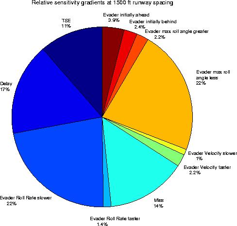
42 Figure 3-4. Relative sensitivities 28

43 From the pie charts, one may directly obtain the top three parameters exhibiting the greatest sensitivity at each runway spacing. These parameters are presented in Table 3-3. Table 3-3. Top three parameters with highest gradients at each runway spacing 750 ft 1100 ft 1500 ft Most sensitive parameter(s) Safety buffer (18%) Delay (18%) Evader with slower roll rate, Evader with lower bank angle (both 22%) Second most sensitive parameter(s) Third most sensitive parameter(s) Delay (16%) TSE (14%) Evader with lower slower roll rate (17%) Safety buffer, evader with lower bank angle (both 16%) -- Delay (17%) 3.6 Results of Sensitivity Study Overall, the delay time between the onset of the roll rate of the blunderer and the onset of the evader s roll rate significantly influenced the closest point of approach at all three runway spacings. At 1100 and 1500 ft runway separation, ensuring the evading aircraft at least matches the roll rate and maximum roll angle of the blunderer also figures prominently. Minimal advantage is gained by exceeding the blunderer s roll rate and maximum roll angle; however, significant sensitivity is exhibited if the evader fails to match the roll rate and maximum roll angle. At 750 ft, the accuracy of the guidance system becomes more critical. A detailed study of the permissible delay time and the necessary guidance accuracy is presented in the next section Safety buffer Although visual formation flying is safely performed every day, it is because of the large amount of information that the trail pilot has about the lead aircraft that this maneuver may be safely accomplished. In IMC, the safety buffer, typically 500 ft, is factored into maneuvers in order to compensate for a lack of high fidelity information about the neighboring aircraft. While any blunder is a fundamentally dangerous scenario for neighboring aircraft, this event occurs so rarely that no cases of a blunder during an IMC parallel approach have ever been officially documented. Anecdotal evidence suggests that blunders have occurred 29

44 and, therefore, two fundamental capabilities must be given to pilots performing UCSPA: 1) the ability to fly a very precise, high integrity approach to landing and 2) the activities of the adjacent aircraft to sufficient detail that a successful escape maneuver may be accomplished should the other aircraft blunder. When these two capabilities exist, then the safety buffer may be reduced Heading Change While the maximum allowable heading change was fixed at 45 deg for the evader, the closest point of approach typically occurred near the point where both aircraft were on parallel courses with a 30 deg heading change. Therefore, it is important that the evader aircraft match the heading change by the blundering aircraft, but it is not critical that the evader aircraft exceed the blunderer s heading change. 3.7 Trade-off Studies Having gained an understanding of which parameters affect the miss distance most significantly, the values of the parameters may then be cross-plotted to determine the trade-off in capabilities with respect to miss distance. Since delay time was determined to be significant at all runway spacings, it is presented in all of the following surface plots. For each tradeoff study, the parameters of interest were varied about the baseline trajectory presented in Table 3-1. The first study is presented in Figure 3-5 which gives a composite view of three parameters for runway spacings of 700, 1100, and 1500 ft. The x-axis is delay time in seconds, the y-axis is TSE in feet, and the z-axis is runway spacing, in feet. The colors at each runway spacing correspond to the centers of mass separation (f from Eqn 3-13), with dark red indicating a collision and dark blue indicating a miss distance of more than 500 feet. From this four dimensional plot, one may assess the design space when determining permitted delay time and necessary guidance accuracy for desired runway spacing and miss distance. Note that the centers of mass separation colors correspond to a distance between two point masses. To determine the miss distance of two actual airplanes of the same type, the largest dimension of that type must be considered. For example, the fuselage of the B is almost 232 ft long, longer than its wingspan. In Figure 3-5, for two B s to avoid 30

45 collision, the centers of mass separation would need to be at least 232 ft, corresponding to orange. Table 3-4 lists the distances between centers of mass for various aircraft. Table 3-4. Distance between the centers of mass of two airplanes Airplane Model Centers of mass miss separation to avoid collision B-747X 264 ft B ft B ft B ft B ft A ft A ft A ft Figure 3-5. Parametric trade-off between TSE, delay time, and centers of mass separation separation, ft 31

46 As an example, suppose two, B s were on approach to runways spaced 700 ft apart and it was desired to have a 200 ft safety buffer between aircraft during a blunder. This means that the desired center of mass separation is 113 ft plus 200 ft, a total of 313 ft, which corresponds to orange on the color bar. At 700 ft, one may trace the orange contour and note that if each aircraft had a 100 ft TSE toward the other, the maximum permitted delay time is 2 sec. With a 50 ft TSE, the delay time increases to 3.5 sec. The direct trade-off between precisely positioning the aircraft and the time to respond is readily apparent. Implicit in this study is the assumption that the evader has perfect knowledge of the blunderer s position, velocity, and attitude Additional Trade-off Studies Surface plots are presented in Figure 3-6 to Figure 3-9 for the other parameters of interest. In each case, the unvaried parameters remained at their baseline values. The baseline trajectory specification is repeated here for reference. Table 3-5. Baseline trajectory start time, sec Roll rate, deg/s Max roll angle, deg Max heading change, deg Airspeed, kts TSE, ft Initial longitudinal separation, ft t 0 Blunderer Evader t Figure 3-6 presents the effect of initial longitudinal offset between the two aircraft. In the nominal case, the blundering aircraft began its maneuver while abeam the evader aircraft. By varying the initial offset between plus and minus 500 ft, the effect of initial position versus delay time shows that the most dangerous position is for the blundering aircraft to be ahead of the evader. If the blunderer is at least 250 ft behind the evader initially, the blunderer will turn behind and be no factor to the flight path of the evader, regardless of the evader s response. 32

47 Figure 3-6. Effect of initial longitudinal offset and delay time ahead behind Figure 3-7 and Figure 3-8 present the effects of relative maximum roll angle and roll rate, respectively. The separation distance contours are very similar in shape, illustrating the basic principle that it is always better for the evading aircraft to roll further and at a faster rate than the evader. It is critical for the evader to at least match maximum roll angle and roll rate, however, it is only marginally beneficial to exceed the blunderer s parameters. It clearly is dangerous to either not have the information to match the blunderer s parameters or to not have the aircraft capability. This need for performance matching may require the pairing of similar aircraft for ultra closely spaced parallel approaches. 33

48 Figure 3-7. Effect of the difference between maximum roll angles and delay time Figure 3-8. Effect of difference in roll rates 34

49 Figure 3-9 presents the effect of different aircraft approach speeds, varying between plus or minus 20 knots of the nominal 130 kts. Recall that the aircraft are initially abeam each other. The worst case occurs when the evader is slower than the blunderer, within this range of airspeeds. If the evader is faster, they are more likely to outrun the blundering aircraft. The data indicates that if the approach speeds differ by more than 30 kts, the likelihood of collision is substantially reduced. The only danger then would be the resulting longitudinal separation during the course of the approach and the potential for hazardous wake vortex conditions. Figure 3-9. Effect of difference in airspeeds and delay time 3.8 Conclusions This parametric sensitivity study has determined that the delay time between the onset of the roll rate of the blunderer and the onset of the evader s roll rate significantly influenced the miss distance at all three runway spacings. This delay time includes the pilot or autopilot reaction time, the collision detection and resolution algorithm computational time, any delay incurred by the electronics, and the dynamics of the aircraft. Assuming the existence of an air-to-air data link, the fast response times (< 5 sec) required at runway separations 35

50 less than 1100 ft will require either new displays for pilot-in-the-loop operations or distributed, intelligent auto-pilots with high-integrity collision detection algorithms that automatically execute the emergency escape maneuver. An intelligent auto-pilot combination may be envisioned whereby the individual auto-pilots of the two aircraft are coupled via data link and the pilots monitor the approach with a different display. Although the ADS-B specifications [35] call for a two Hz update rate with 50% probability of reception, effectively making it, on average, a one Hz data link, it is clear that ultra closely spaced parallel approaches would benefit from guaranteed update rates of two Hz or better during the approach. At 1100 and 1500 ft runway separation, ensuring the evading aircraft at least matches the roll rate and maximum roll angle of the blunderer also figures prominently. This brings up the issue of requiring similar aircraft for ultra closely spaced parallel approaches. If a light commuter aircraft was to aggressively blunder toward a fully loaded heavy transport, it is unlikely that the heavy could match the commuter s roll angle and roll rate, and to do so in a timely manner. Given the criticality of these two parameters, aircraft with similar performance capabilities should be paired, particularly with a runway spacing less than 1500 ft. At 750 ft, the accuracy of the guidance system is second in importance only to the delay time. Controlling Total System Error to better than 100 ft for each aircraft allows delay times up to 3 seconds, which is aggressive, but achievable if the auto-pilots of the individual airplanes are coupled via a high update rate data link and automatically execute the escape maneuver. To limit total system error to less than 100 ft for pilot in the loop operations will require new displays, such as the tunnel-in-the-sky display, as well as a differential GPS for navigation. With a modern auto-pilot coupled for the approach, 100 ft of total system error may be obtained using either the instrument landing system or a differential GPS system for guidance. Both of these scenarios presume relatively low atmospheric turbulence on the final approach course. Further data on total system error is presented in the next chapter. 36

51 Chapter 4 Visual, Cruise Formation Flying: Pilot Response Time In the previous chapter, the parameters critical to the success of ultra closely spaced parallel approaches were identified. Next, we explore ways of determining actual or expected values of these parameters. We begin by investigating the parameters governing the accepted procedure of visual parallel approaches. Although ultra closely spaced parallel approaches (UCSPA) are not permitted in instrument meteorological conditions (IMC), they are allowed in visual meteorological conditions (VMC) with the pilots providing separation assurance. Assuming then that a pilot s response to an encroaching aircraft in visual conditions is acceptable for safety, one may quantify this response and use it as a baseline for acceptable response to a blunder in instrument conditions. Executing an ultra closely spaced parallel approach closely resembles loose formation flying as each aircraft attempts to maintain a minimum acceptable spacing relative to the adjacent aircraft while also flying a straight-in approach to the runway. Thus, an experimental evaluation of pilot-in-the-loop, dual aircraft cruise formation flying system dynamics in VMC was undertaken to examine pilot response time and system frequency response characteristics. These characteristics will then be used as a basis for modeling pilot response behavior during a blunder. Other researchers have investigated optimal performance of close formation flying; however, there has been little experimental research on the characteristics of piloted, cruise (> 100 ft separation) formation flying [36][37]. One key concern in collision avoidance during a blunder in IMC is the delay time between when the blunder starts and when the evading pilot commences the escape maneuver. In other words, how long does it take for the pilot to 1) determine that the other aircraft has maneuvered and 2) maneuver their own airplane in response. In visual formation flying, the 37

52 pilot is responsible for both collision detection and resolution. The envisioned scenarios in IMC are: 1) a computer-based on-board collision detection algorithm to alert the pilot to a potential collision who then either manually or with the auto-pilot engaged, executes the escape maneuver and/or 2) for the pilot to have a display showing the neighboring aircraft position and attitude, thus enabling human collision detection, as in visual conditions. Since visual parallel approaches are performed daily, the question is, how fast does a pilot respond to another aircraft maneuvering towards them and what parameters affect this response time? We may then use this information to model realistic pilot-in-the-loop response times and to baseline the response time of the human collision detection and resolution algorithm against that of a computer-derived algorithm. The primary variables of interest in determining pilot response time are the specific maneuver of the blundering aircraft and the initial separation distance. In order to determine the pilot reaction time as a function of adjacent aircraft maneuver, a series of two airplane formation flights were conducted in which various single axis maneuvers such as roll inputs, pitch changes, and wings-level yaw were performed by the lead aircraft. The trail pilot s task was to attempt to maintain the current separation distance by following the lead s maneuver, thus requiring the trail pilot to accurately diagnose and anticipate the lead aircraft s intent. These maneuvers were then repeated at different ranges in order to also model the pilot s response as a function of initial separation distance. 4.1 Flight Test Setup Three formation flights were performed using a Beechcraft Queen Air as the maneuvering, lead airplane and a Cessna Caravan as the evading, trail aircraft. The same pilots flew each airplane for all flights. In addition to the three formation flights, a solo parameter identification flight with the Caravan was performed to gather dynamic response data Definitions Throughout this chapter, reference will be made to aircraft pitch, roll, and yaw angles, their angular rates, and ground track angle. Aircraft pitch, roll, and yaw angles are illustrated in Figure 4-1 and are the Euler angles which define the motion of the aircraft body coordinate frame relative to the earth-fixed, inertial frame. In this document, angular rates are denoted 38

53 by the angle with a dot over it, such as φ for roll rate, in rad/sec. Ground track angle, a parameter referenced extensively in the following analysis, is defined by Eqn 4-7. Figure 4-1. Definition of Euler angles. Photo courtesy of Raytheon Instrumentation The Queen Air and Caravan both had a prototype Wide Area Augmentation System (WAAS) installed to produce differentially corrected GPS position and velocity. The WAAS system broadcasts corrections from a geosynchronous satellite at the rate of one Hz on the L1 frequency (1575 MHz). A Novatel Millennium receiver passed GPS and WAAS correction messages to a Stanford University algorithm [38][39] at a rate of 4 Hz which then calculated corrected aircraft position and velocity. All of these flights were performed prior to the removal of selective availability from the GPS signal. During the formation flights, the Queen Air (lead aircraft) also had a Honeywell HG1150 Inertial Navigation System (INS) installed which recorded roll, pitch, and heading angles at up to 50 Hz. For the parameter identification flight, the INS was installed on the Caravan. Control surfaces were not instrumented nor were the yoke or rudder pedals. Video footage was acquired during the second formation flight Formation Flight Procedure The nominal Caravan test conditions were 4000 ft MSL and 130 kts. The Queen Air flew at 3900 ft at the Caravan s 9 to 11 o clock position. A block of up to seven test points were given to both pilots and the Queen Air pilot randomly chose the order. Each test point was 39

54 performed twice (not consecutively) at each separation distance. Nominal initial lateral separation distances tested were 2500, 2000, 1700, and 500 ft. In order to ensure safety, but avoid predictable maneuver times, ready for maneuver calls would be confirmed by both pilots and at some time subsequent to those calls, typically five to twenty seconds later, the lead pilot would maneuver the Queen Air. Roll and yaw maneuvers discussed in the following sections are for maneuvers only toward the trail aircraft Parameter Identification Flight A separate flight with only the Caravan was performed in order to gather data on the Caravan s dynamic response. Using this data, one may then identify appropriate time constants and frequencies, which were then used in post-processing the pilot response times. Step and hold inputs as well as doublets were performed to gather data on roll mode time constant, steady state roll rate, dutch roll characteristics, and pitch dynamics. Data on long period phenomena such as phugoid and spiral divergence were not obtained. 4.2 Pilot Response Time A block diagram of the dual airplane formation flying system is presented in Figure 4-2. With instrumented yokes, the pilot response time would simply be the time difference between the pilot yoke inputs. The aircraft used in this experiment did not have instrumented yokes because certification constraints prevented it. Thus, the aircraft response must be separated from the pilot response analytically. Figure 4-2. Block diagram of formation flying dynamics To separate pilot response time from the total response of the pilot/aircraft combination to the lead aircraft maneuver, the aircraft dynamics for a particular maneuver, say a roll, were 40

55 modeled. Using WAAS velocities, one can determine the ground track angle change as a function of time for a roll at various roll rates. Ground track angle change is defined as instantaneous change in ground track from the initial ground track direction. Mathematically, it is the arctangent of the ratio of the two dimensional components of GPS velocity at each point in time (see Eqn 4-7). If it takes two seconds for a Caravan at 4000 ft and 130 kts to change its ground track angle by half of a degree (0.5 deg) while rolling at 9 deg/sec (this is strictly a function of aircraft dynamics), and the total time recorded for the pilot/ aircraft combination to change ground track angle by 0.5 deg is three seconds, then one may say that the pilot response time for this maneuver is one second. For these flights, a ground track angle change of 0.5 deg was chosen as the critical point for two reasons: 1) the signal to noise ratio of WAAS velocity could clearly capture this small change in angle and 2) it is more accurate to estimate pilot response time early in the maneuver before other factors such as wind, unmodeled aircraft dynamics and station keeping factors all become significant. Note that ground track angle is different from flight path angle when wind is present. For a maneuver such as a climb and descent, a height change of 2 meters was chosen for identical reasons Roll Angle Change Maneuvers As an example of removing aircraft dynamics from the total system response, let us examine flight test maneuvers that had a significant roll angle change component: rolls (15 and 30 deg) and climbing turns. Only turns toward the flight path of the trail aircraft were analyzed. A representative ground track is presented in Figure 4-3, where the x-axis is time and the y-axis is change in ground track angle, which was derived from WAAS-based instantaneous velocity measurements. In order to back out the pilot s response, the roll dynamics of the Caravan must be accurately modeled and the various errors sources determined and quantified. 41

56 Figure 4-3. Queen Air and Caravan ground track angles during a right roll Caravan Roll Dynamics One flight was performed in order to estimate the dynamic response of the Caravan at the test conditions of the formation flight: 130 knots and 4000 ft. Step inputs and doublets were used to excite the various modes, with time history data being recorded at approximately 50 Hz by the Honeywell HG1150 INS. Based on the data obtained, the roll mode time constant and steady state roll rate were determined, which in turn were used to generate predicted flight path trajectories. Beginning with the linearized, small perturbation aircraft dynamic equations of motion [40], assuming x-z plane symmetry and simple roll without perturbation in the other axes: L L δa + p = φ Ix 4-1 δ a p where L is rolling moment, is aileron deflection, p is roll rate, is moment of inertia about the x axis, and φ is roll angle. ( L δ a ) δ a is the roll moment due to the deflection of the ailerons and ( L p) p is the roll-damping moment [41]. Eqn 4-1 may be rewritten as δ a I x 42

57 τ p + p = L δa δ a L p 4-2 where τ 1 L p L δ = and L p = and L a δa = L p I x and τ is defined as the roll mode time constant. The time constant indicates how quickly the airplane will reach a steady state roll rate given a step input in aileron deflection. For a step change in aileron deflection, Eqn 4-2 may be analytically solved to produce I x 4-3 p() t L δa L p As t->, the steady state roll rate becomes = ( 1 e t τ ) δ a 4-4 p ss L δa = δ a L p Substituting this expression into Eqn 4-4 results in an expression for roll rate as a function of time with only two unknowns: the time constant, τ, and the steady state roll rate, p ss : p() t = p ss ( 1 e t τ ) Using this expression and a step input in aileron deflection, a time history of roll rate may be generated during flight test [42] from which and τ may be determined. With different aileron deflections, a family of roll rate time histories would be generated since each aileron deflection produces different steady state roll rates. For the flight test, an approximately constant amplitude step input in aileron was performed by marking the desired yoke input on the yoke housing. Time histories of two roll events are shown by the dotted lines in Figure 4-4. From this time history, a steady state roll rate of 18 deg/s and a time constant of 0.5 sec were calculated, which produced the modeled roll response (the solid line). p ss

58 Figure 4-4. Experimental and modeled Caravan roll response to a step aileron deflection. Using this modeled data of roll response and Eqn 4-7, ground tracks were produced that model how the Caravan would respond to a roll input with no pilot delay. All integrations were performed using a variable step size, fourth order Runge-Kutta method. t - τ φ() t = p 1 e dt ss g ψ() t = V --- tan φ () t dt V y () t = Vsinψ() t 4-7 Assuming the roll mode time constant remains the same regardless of the aileron deflection, the steady state roll rate, p ss V x () t = Vcosψ() t V y ground track angle = atan V x,was varied between 5, 9 and 18 deg/s and the resulting ground track angle change is plotted in Figure 4-5 for a specific ground speed of 130 kts. These curves will change as a function of ground speed. In order to model values of ground track angle change due to aircraft dynamics only, ground speed was calculated at each test point 44

59 during the formation flight, thus enabling specific ground track angle change models to be calculated at each test condition. Figure 4-5. Modeled Caravan ground tracks for various steady state roll rates at 130 kts groundspeed = 130 kts time to 0.5 deg without pilot delay Specifically, at 130 kts ground speed, without pilot delay and a steady state roll rate of 9 deg/sec, the modeled Caravan time to a ground track angle change of 0.5 deg is approximately 1.25 sec, as shown in Figure 4-5. The total time to 0.5 deg during the formation maneuver presented in Figure 4-3 is approximately 2.5 sec. Using the simple formula in Eqn 4-8, pilot delay time = total measured time to 0.5 deg modeled Caravan time to 0.5 deg the calculated pilot delay time would be 2.5 sec sec = 1.25 sec. 4-8 Since roll rate was not available on the trail airplane during the formation flights, an estimate of 9 deg/s was used for modeling purposes. This is based primarily on the measured, average lead aircraft roll rate of 9 deg/s. Allowing for the range of actual roll rates to be within plus or minus 3 deg/s of the nominal 9 deg/s, errors of +0.3 sec and -0.1 sec are possible. This effectively translates to a pilot delay time error of +0.1/-0.3 sec. 45

60 WAAS Velocity Accuracy Since WAAS is being used as the primary flight path sensor, one must account for WAAS velocity inaccuracy in assessing the final error of the pilot response time. WAAS velocity accuracy was measured using data taken from a static antenna. The velocity of the antenna should always be zero, so any indicated WAAS velocity may be modeled directly as noise. The following table presents WAAS velocity errors from data gathered over 15 hours at Stanford. Relative to the ground speed of about 67 m/s, the error in ground track caused by the inaccuracy of WAAS velocity is negligible. Table 4-1. WAAS velocity errors 68th percentile (m/s) 95th percentile (m/s) East North Up INS time versus GPS time The two primary sensors used in these tests, the INS and WAAS, did not share the same time stamp on the data for the first two flight tests. In the first two flights, the INS data was tagged with an arbitrary time stamp and manually aligned with GPS data. WAAS and INS velocities were plotted on the same time history (east and north velocities only), the velocities were then manually lined up and the time difference recorded. This time change was then applied to all of the INS data. The error associated with this manual process is within +/ sec. On the third flight test, one computer housed both INS and GPS interface cards and the INS data was tagged with GPS time Determining the Start Time of the Lead Maneuver The start of the lead aircraft s maneuver was defined to be the point at which roll angle begins to change from its steady state value just prior to the maneuver. The determination of the time of roll angle change was performed manually and is estimated to be accurate to within +/- 0.1 sec Summary of Roll Response Errors From the preceding discussions, the following list summarizes the estimated, maximum error for each of the components contributing to the overall error. 46

61 Mismodeling of Caravan roll dynamics: +0.3/-0.1 sec Airspeed vs. ground speed: +/ sec WAAS velocity inaccuracy: negligible INS/GPS time alignment: +/ sec Start of Lead Maneuver: +/- 0.1 sec In order to give some indication of the measurement accuracy, the errors are added and result in maximum error bounds on the calculated pilot response times. Maximum error bound on pilot response to roll maneuvers: +0.3/-0.5 sec Pilot Response Results for the Roll-Towards-Trail Maneuvers Figure 4-6 presents pilot response time as a function of separation distance and type of roll maneuver: roll to 15 or 30 deg and climbing turns. Below 2000 ft separation, the pilot response time to the roll maneuver generally shows no particular trend; the pilot usually responds in less than 2 sec, with an average time of about one second. For the case of the lead aircraft rolling to 30 deg, there is a trend with distance and the solid line shows the best fit for that set of data. The polynomial equation for the curve fit is expressed as t = e 7 d e 4 d where t is pilot response time in seconds and d is separation distance in feet

62 Figure 4-6. Pilot response times versus rolling maneuver and separation distance Curve fit is for 30 deg roll only Response to Climb and Descent Maneuvers The approach to separating aircraft response from pilot response time for climbs (and descents) is different from that employed in separating roll dynamics. Climb dynamics are a function of not only pitch and pitch rate, but static stability and angle of attack. As such, simply using pitch angle and a time constant does not adequately describe the motion of the airplane. Instead, an approach using the conservation of energy was employed which enabled better prediction of aircraft time to climb Determining Aircraft Pitch Response For a given initial specific energy, the time to reach some predefined change in height may be measured by performing step inputs in elevator. This time would then be subtracted from the combined pilot/aircraft response to isolate the pilot response when responding to a climb or descent maneuver during formation flying. This method is reasonable for up to about three seconds after the climb or descent is initiated. After that, induced drag becomes 48

63 significant and conservation of energy is no longer valid. Specific energy, or energy per unit mass, is defined by where E is the energy, m is the mass of the aircraft, V is the airspeed, g the gravitational constant and 4-10 is the change in height of the aircraft. For this flight test, airspeed as a function of time was not recorded; however, three-dimensional groundspeed was recorded. The initial airspeed was manually recorded for each test point and from this, one may calculate the initial specific energy just prior to the maneuver: where V i h E = --V i = constant is the initial airspeed. Since the initial airspeed was the same for each maneuver in each flight test, this expression will be the same regardless of change in aircraft weight, since energy required to reach the initial airspeed will increase proportionally. Substituting Eqn 4-11 into Eqn 4-10 and re-arranging results in In order to calculate --- E m 4-12 Vt (), the windspeed is determined by subtracting the known initial airspeed (in this case, 130 kts) from the calculated three dimensional WAAS groundspeed. At each time step then, the windspeed is removed from the calculated groundspeed before determining change in altitude resulting in h() t This calculated change in altitude may be compared with actual change in altitude measured by WAAS during step inputs in elevator. Figure 4-7 shows a comparison of actual versus calculated altitude change. = h() t 1 --V() t 2 + g h() t g 2 --V 1 = i --V() t g 2 --V 1 = i -- ( V 2 g () t V wind )

64 Figure 4-7. Modeled versus actual change in height during step elevator input For this maneuver, the model matches the data within 0.2 sec at the 2 m mark, giving a confidence check on the WAAS vertical position measurement. Using the data, the time to a height change of 2 meters exclusive of pilot delay is 1.53 seconds. This time will then be subtracted from the time to 2 meters during the formation flying maneuver. Although total airplane weight changed from flight to flight, the specific energy did not, so this delay time will be valid for all maneuvers begun at 130 kts. The additional parameter which did change and will affect the delay time is static margin, which is a function of aircraft center of gravity. A weight and balance was performed for each flight configuration and the center of gravity moved forward for the three formation flights by up to 3.7 inches. This will result in the aircraft response to elevator input being slightly longer; however, since the change in center of gravity location is so small, this effect will be neglected for the pilot response studies. Figure 4-8 shows the model of a pushover or descent maneuver. Time to a change in height of 2 meters was averaged between the two data sets and determined to be 1.15 seconds. 50

65 Figure 4-8. Model of aircraft response to a pushover Pilot Response to Climb and Descent Maneuvers Pilot response time as a function of separation distance and pitch maneuver is shown in Figure 4-9. Approximate error is +0.10/-0.25 sec, based on an analysis similar to that detailed in Section A second order polynomial curve fit is also presented for climbing and descending maneuvers. One can see that the response to a climb is quicker than to a descent, but that responses to both do slightly increase with increasing separation distance. Climb response may be represented by the second order polynomial shown in Figure 4-9 and written as t = e 7 d e 4 d where t is pilot response time in seconds and d is separation distance in feet. Pilot response to pushovers may be expressed as t = e 7 d e 4 d Eqn 4-14 and Eqn 4-15 are used to illustrate the trends of climbing and descent maneuvers and may be used in future models of pilot response time

66 Figure 4-9. Pilot response to pitch-type maneuvers Response to Wings-Level Yaw Maneuvers The final class of maneuver performed in formation flying was a wings level yaw, with varying maximum yaw angle. Although such maneuvers are rarely performed during normal flight operations, they may represent the effect of an aircraft drifting or a sideslip maneuver during a glideslope recapture Aircraft/Pilot Response to Yaw In the case of yaw, the pilot was not accustomed to making a pure rudder input as a response and would typically respond with a combination of roll and yaw. Since the response was variable, it is very challenging to accurately remove the airplane response without an INS on the Caravan to record aircraft attitude. For this analysis then, it is presumed that the trail pilot made a roll-only input, thus enabling us to use the procedure outlined for the roll maneuvers. Using these results, Figure 4-10 presents the pilot response characteristics to a 1/4 or 1/2 of maximum rudder pedal input by the lead aircraft. The error estimate is approximately -0.4/+0.4 sec, again, following an analysis similar to that presented in 52

67 Section The larger errors are due to the presumption of a roll-only response to the yaw maneuver. Figure Pilot response to wings level yaw maneuvers no pilot response The feature unique to this series of maneuvers is that the trail pilot did not respond to five out of the eleven maneuvers. Although the pilot responded to all of the maneuvers occurring around 500 ft separation, at distances greater than 1500 ft, he could only perceive changes in either attitude or spacing 37.5% of the time. In this case, it appears that maneuver maximum amplitude is critical to successful yaw identification, a phenomenon that was not exhibited by the roll or climb/descent maneuvers. 4.3 Summary of Pilot Response Results A composite graph of the data from the previous sections is presented in Figure Error bars generated around each test point delineate the possible range of pilot response. One can see that the pilot generally responds the fastest to roll angle changes, followed by pitch changes, and is the least responsive to heading angle changes. Both pitch and heading angle changes exhibit some sensitivity to separation distance; however, pilot response to roll angle change at separation distances less than 2000 ft is consistently less than 2 seconds. Above 2000 ft, pilot response is slower by half a second, but the quantity of data 53

68 above 2000 ft is significantly lower than that below 2000 ft and additional data should be obtained before direct comparison made. Figure Composite of pilot response times with error estimations no pilot response 4.4 Conclusions The preceding analysis suggests that a pilot discerns roll angle change more quickly than either pitch or yaw angle changes. This response time averages about one second for separations less than 2000 ft. Response to a climb maneuver is faster than that to a descent and is probably because pitching the nose up to climb is a more natural response than pushing over in order to descend. Pilot response to a wings-level yaw maneuver is between one and five seconds, but frequently there is no response at all. This series of flights forms a basis for analyzing pilot response; however, additional issues such as individual differences in pilot response, differences in lead aircraft maneuver entry characteristics, and atmospheric factors such as sun angle, background terrain, and cloud coverage have not been addressed. The superior trail pilot response to lead aircraft roll maneuvers compared to yaw maneuvers strongly suggests that roll information is valuable 54

69 to the pilots for collision avoidance in situations such as ultra closely spaced parallel approaches and thus, should be included in any air to air data link. 55

70 Chapter 5 Visual, Cruise Formation Flying Dynamics The previous chapter quantified pilot response time to maneuvers performed during visual, cruise formation flying. In this chapter, the same data sets were used to analyze the overall dynamics of a two aircraft, pilot-in-the-loop cruise formation flying system. The system dynamics will then indicate the trail pilot s ability to accurately track and respond to the maneuver of the lead aircraft, thus creating an analytical model of the dynamics of the human collision detection and resolution algorithm. One way to create a system model is to use experimental data along with system identification techniques to model the overall dual aircraft system dynamics. The input to the system is the lead aircraft maneuver while the output of the system is the trail aircraft s response. This chapter follows that approach and describes the system identification methods in detail as applied to example data gathered from a lead aircraft abruptly rolling towards the trail aircraft. The merits of both single input/single output and multiple input/ single output models were analyzed and the resulting models validated in order to determine the necessary information required to satisfactorily anticipate system behavior. This information must then be present in any air-to-air data link designed for cooperative, multi aircraft cruise formation flying. 5.1 Physical model of Formation Flying A simplified physical model of formation flying is the spring-mass-damper system illustrated in Figure

71 Figure 5-1. Physical basis of formation flying model The airplanes are modeled as point masses and assuming no external forces (primarily wind in the case of flight), the linear equation of motion for the x-direction is m 1 x 1 + bx 1 + kx 1 = m 2 x 2 + bx 2 + kx where x 1 and x 2 are deviations of the aircraft from their nominal positions, 1 is the mass of the lead aircraft, m 2 is the mass of the trail aircraft, b and k are damping and spring coefficients, respectively, and x, x, and x are acceleration, velocity, and position. Solving for x 2, the trail aircraft position, and accounting for the fact that the trail aircraft pilot response time to a lead aircraft maneuver will be delayed by α seconds, the generalized formation flying model may be written: x 2 () t = ax 2 ( t α) + bx 1 ( t α) + cx 1( t α) + dx 1( t α) + fx 2() t + gx 2() t where a, b, c, d, f, and g are generalized linear coefficients and α is the trail pilot response time. Note that b now refers to a generalized coefficient rather than the damping coeffcient. Performing a Laplace transform and rearranging the equation into transfer function form results in: X 2 ( s) be αs + cse αs + ds 2 e αs = X 1 ( s) 1 fs gs 2 ae αs where the input, X 1 ( s), is the lead aircraft position and the output, X 2 ( s), is the trail aircraft position. Using a first order Pade approximation for the delay, 5-2 e αs the transfer function may be rewritten as 2 αs αs 5-4 X 2 ( s) = X 1 ( s) αds 3 + ( 2d αc)s 2 + ( 2c αb)s + 2b αgs 3 + ( αf 2g)s 2 + ( α+ αa 2f)s +( 2 2a)

72 Using this form of the transfer function and data from carefully controlled experiments, a variety of parameter identification methods may be used to estimate the values of the coefficients. The values of these coefficients determine the system dynamics. 5.2 Parameter Identification Example The experimental formation flying setup is described in detail in Chapter 4. In summary, two aircraft flew in formation at nominal conditions of 130 kts and 4000 ft at some predetermined initial lateral separation distance. The lead aircraft would then execute an abrupt maneuver toward the trail aircraft for 10 to 20 sec. This maneuver would be either in the roll, pitch or yaw axis. The trail pilot was tasked to mimic the maneuver and attempt to maintain the initial separation distance. The maneuver concluded when the lead aircraft removed the input and resumed straight and level flight. Over the course of three formation flights, maneuvers in all three axes were performed at initial lateral separation distances varying between 500 and 2500 ft Two example maneuvers were chosen to illustrate the parameter identification (PID) techniques. The first was the lead aircraft executing an abrupt roll to a roll angle of 15 deg towards the trail airplane from an initial separation distance of 1900 ft. The second was the lead aircraft executing an abrupt roll to 30 deg towards the trail airplane from an initial separation distance of 500 ft. Two data sets were taken at each test point, one with which to estimate the parameters and the second for model validation. The primary variables of interest were velocity, provided by the Wide Area Augmentation System (WAAS), and attitude, provided by a Honeywell navigation grade inertial navigation system installed on the lead aircraft. In system identification, it is important to capture all of the system dynamics, yet avoid including the process or measurement noise. Most parametric models handle this by estimating the noise dynamics separately. This separation between system and noise dynamics becomes increasingly challenging as the signal to noise ratio decreases. Fortunately, because of the excellent signal to noise ratio of WAAS velocity in this application (approximately 100:1), the error dynamics are negligible. Thus, a relatively simple parameter identification model, the Auto-Regression with extra inputs (ARX) model, provided good modeling of the formation flying system dynamics. In the ARX model, the current esti- 58

73 mated output is a linear function of the past inputs and outputs. In most cases, a second order ARX model with a two-step time delay exhibited the best fit for the physical system [43]. The ARX model form may be described by Ay = Bu + e 5-6 where y is the output vector, A is the output vector coefficient matrix, u is the input vector, B is the input vector coefficient matrix, and e is the noise. For a second order model with a two step time delay, the resulting discrete transfer function is of the form b Gz ( ) 0 z + b = zz ( 2 + a 1 z+ a 2 ) The Tustin approximation (trapezoidal rule) was used to convert the transfer function to the continuous time domain. At each separation distance, a best model was then created to fit the dynamics of the formation flight system for a particular maneuver. In this example case of the lead aircraft executing a 15 deg roll toward the trail aircraft, the best fit ARX model may be expressed as X 2 ( s) s s s = X 1 ( s) s s s where X 1 is the ground track angle of the lead aircraft and X 2 is the ground track angle of the trail aircraft. The ground track angle effectively translates two dimensional position information into a single variable by using the ratio of the instantaneous velocity vector components ground path angle = V y atan V x 5-9 where V y is the component of the aircraft velocity in the y direction and V x is the component of the aircraft velocity in the x direction. The ground track angle of each aircraft at the beginning of the lead aircraft s maneuver is subtracted out, effectively making X 1 and X 2 changes in ground track angle. The pilot response time may be extracted by comparing Eqn 5-5 with Eqn 5-8 and solving for the pilot response time, α. To do this, α must be iteratively chosen in order to create a linear system in a, b, c, d, f, and g. The best solution then corresponds to the α which produces the lowest root sum square of the errors. Once α is 59

74 chosen, we have eight equations and six unknowns, so the system is overdetermined and a least squares solution may be used. Forming the linear system, Hx + m = y α α α α α 2 α where x contains the solution vector [a b c d f g] from Eqn 5-5, H contains the coefficients of the solution vector, m contains constants, and y comes from the coefficients in Eqn 5-8. A range of values of α was chosen and using a least squares method to solve for x, xˆ = ( H T H) 1 H T y 5-12 where xˆ is the estimation of x. For each value of α, the root sum square of the errors, x - xˆ, was calculated. The α which results in the lowest root sum square error is the best solution to the linear system. As illustrated by Figure 5-2, the resulting best solution for the coefficients a, b, c, d, f and g corresponds to Figure 5-2. Root Sum Square error vs. pilot response time, alpha a b c d f g α 2 α = 0.3 = sec

75 There is an additional near-minimum at With α =0.3, the resulting solution vector is α = 0.5 ; however it is not the global minimum. Comparing the calculated pilot delay time of 0.3 sec with the pilot delay time determined in Chapter 4 for a lead roll to a roll angle of 15 deg toward the trail aircraft at 1900 ft separation, one can see that this falls well within the range of 0.4 sec +0.5/-0.3 sec, thus providing a secondary check between two entirely different methods of calculating pilot response time. a b c d f g = Single Input vs. Multi-input Modeling The first parameter identification was performed using the ground track angle change of each aircraft in a single input/single output (SISO) model. This model is simple and the data readily available to any aircraft equipped with WAAS or other precise positioning system. With selective availability now turned off, even stand-alone GPS may be sufficient for this analysis. However, given the assumption that the pilot likely senses roll angle change as the first indication of a roll maneuver, pilot in the loop formation flying may be better modeled by using multiple inputs, i.e., ground track angle and roll angle. This situation creates a multi input/single output (MISO) system where the lead aircraft s ground track angle change and roll angle are the inputs and the trail aircraft s ground track angle change is the output. The MISO system was also modeled using a second order ARX model where the input is now a matrix of values rather than a vector Residual Error Analysis The residual error is defined as the difference between the actual and modeled system output. In order to determine the goodness of the model, the residuals should be a normally distributed, white noise process with zero mean that is uncorrelated with past inputs. 61

76 To determine if the residuals are a white noise process and uncorrelated with past inputs, an output auto-correlation of the residuals and a cross-correlation of the residuals with the inputs, respectively, may be performed. The auto-correlation is defined as N 1 Rˆ ε = --- N ε()εt t ( τ) 5-14 t = τ where N is the number of data points, τ is the delay time, and ε is the output residual. The cross-correlation is N 1 Rˆ εu = --- N ε()ut t ( τ) 5-15 t = τ where u is the input value. To determine if the residuals are small enough, one may define a confidence interval for a normal distribution whereby if all of the residuals fall within the 99% confidence interval, one may say that the residuals are gaussian and all fall within three sigma of the mean. In order to determine the best model for the second example, that of the lead aircraft rolling to a roll angle of 30 deg towards the trail at an initial separation distance of 500 ft, the two SISO cases and one MISO case presented in Table 5-1 were modeled: Table 5-1. Parameter identification models tested Case Input 1 Input 2 Output 1 Lead aircraft ground track angle -- Trail aircraft ground track angle 2 Lead aircraft roll angle -- Trail aircraft ground track angle 3 Lead aircraft ground track angle Lead aircraft roll angle Trail aircraft ground track angle Not only does a model have to exhibit acceptable residual behavior for the data subsuming the model, but the residuals on the validation data set must also be acceptable. The autoand cross-correlations for the MISO case using the data set used to create the model are presented in Figure 5-3. There are two cross-correlation figures, one for the ground track angle input and the second for the roll input. All of the data lies within the 99% confidence inter- 62

77 val, from which we may conclude that the model adequately captures the highest order dynamics and accurately models the system delays. The residual analysis of the validation data set showed that this model also adequately captured the dynamics of a second roll maneuver at the same separation distance. From this we may conclude that the ARX MISO model adequately captures the formation flight dynamics of a right roll maneuver starting at 500 ft separation distance. Figure 5-3. Auto- and cross-correlation functions for MISO case, modeled data set 63

78 Figure 5-4. Auto- and cross-correlation of MISO model using validation data The residual analysis for the two SISO cases showed slightly poorer modeling performance, but still adequately model system behavior as may be shown in the output analysis Model Output Performance Another means to assess the goodness of the ARX model is to compare the predicted system output with actual system output and examine the average error. Figure 5-5 to Figure 5-7 present modeled and actual output data for the two SISO and one MISO case. In each plot, there are two data sets: the data used for creating the model and the data used for validation. The same ARX model is used to create both predicted system outputs. 64

79 The goodness of fit number presented in each graph is the mean square fit, calculated by fit = norm( ŷ y) ( N) where ŷ is the modeled output value, y is the actual output value, and N is the number of output elements. The SISO models were better at predicting the behavior of the data set used for modeling ( model in the plot); however, the MISO model performed better on the validation data ( validated ). Figure 5-5. Modeled ground track angle change based only on lead aircraft ground track angle change 5-16 Goodness of fit: modeled: validated:

80 Figure 5-6. Modeled ground track angle change based only on lead aircraft roll angle input Goodness of fit: modeled: validated: Figure 5-7. Modeled ground track angle change based on lead aircraft ground track angle change and roll angle Goodness of fit: modeled: validated:

81 5.2.3 Summary of Modeling Techniques The preceding analysis was performed for all lead aircraft test points, covering roll, pitch, and yaw maneuvers at initial separation distances between 500 and 2500 ft. The resulting models are then used to quantify formation flying system characteristics. 5.3 VFR Formation-keeping Characteristics Once the trail aircraft s pilot has determined the intent of the lead aircraft, how well can he or she follow the lead s maneuver? Obviously, for formation flight at distances closer than 50 feet or so, the trail pilot must follow the lead exactly or risk collision. For distances larger than that, there is more uncertainty in diagnosing the intentions of the lead as well as more airspace in which to maneuver. For this test, the trail pilot was instructed to attempt to maintain initial separation distance and to do so, as much as possible, by matching inputs. For instance, if the lead aircraft executed a yaw maneuver, the trail airplane should also execute a yaw maneuver. Formation keeping characteristics, defined as how well the trail pilot could match the lead aircraft s maneuver and maintain initial separation distance, were quantified in terms of the damping ratio and natural frequency of the formation flight dynamics. The characteristics were generated from models created using the parameter identification method outlined in the previous section for the SISO case with lead aircraft ground track angle change being the sole input, except in the case of climb, which used the SISO case with pitch angle being the sole input. From the damping ratio, one may infer how well the trail pilot/aircraft combination can track the maneuver of the lead aircraft. The natural frequency of the system is indicative of the pilot input frequency as well as the aircraft dynamics. At each of the test points, the lead pilot provided a step input maneuver for approximately ten to twenty seconds in one of the different axes: roll, pitch or yaw. As one may see from the following plots, the trail pilot responds quite differently to the different maneuvers. For instance, Figure 5-8 presents a time history of a roll maneuver. The response of the trail aircraft (solid lines) is well damped and the pilot is able to formation-keep on the lead aircraft (dashed lines) well. However, when the lead input is a wing s level yaw maneuver, the trail aircraft ground track is much more oscillatory, as shown in Figure 5-9. The implication is that either the pilot or the pilot/aircraft dynamics combination prevent a well damped 67

82 response to the yaw maneuver. Translating to the frequency domain, one may examine damping ratio and the poles of the system. Figure 5-8. Time history of two roll maneuvers at 500 ft separation Lead Trail Figure 5-9. Time history of two yaw maneuvers, 2300 ft separation Lead Trail 68

83 5.3.1 Roll Tracking Characteristics - Frequency Domain The poles of the open loop formation flying system for roll maneuvers at various separation distances are presented in Figure Roll response is a third order system consisting of a pilot delay time and an oscillatory characteristic. Note that there are overlapping poles at s = -8. Except for the hard right roll at 480 ft, all of the poles have damping ratios between 0.5 and 0.6. The natural frequencies are between 0.3 and 1.1 rad/s, translating to a period of 20.9 sec and 5.7 sec, respectively. In general, the pilot must adjust his formation-keeping position more frequently at further separation distances. Intuitively, this may be due to the need to re-estimate closure rates more frequently and adjust accordingly. The fast pole at s = -8 rad/sec is due to the pilot delay time. Using Eqn 5-5 and Eqn 5-8 and solving for α, one finds that a pole at s = -8 corresponds to a pilot delay time of 0.25 sec, which is very close to the calculated delay time of 0.3 sec of Chapter 4. It is not identical due to the fact that pilot delay is also embedded in the second order response. Figure Pole locations for roll maneuvers at various separation distances Climb Tracking Characteristics - Frequency Domain The formation-keeping characteristics of a climb are presented in Figure 5-11 and demonstrate that the system is primarily composed of pilot delay and a translation mode. 69

84 Figure Frequency response to a climb, normal and zoom view ZOOM If modeled as a second order system, the damping ratio and period is approximately 0.62 and 14 sec, respectively. The short period dynamics, with a time constant of 3 sec and very small amplitude, are not a factor. The pilot is able to estimate and match a climb maneuver with high confidence and accuracy. 70

85 5.3.3 Yaw Tracking Characteristics Since the pilot neglected to respond to roughly half of the yaw test points, there are two possible valid models then for yaw tracking: one that has no response and one that is second order with undamped oscillations. The period of the oscillatory response is approximately 18 sec. Undoubtedly, the dutch roll mode is excited, but the primary factor influencing the light damping ratio of the formation-keeping response is the strong directional stability of the trail aircraft, a Cessna Caravan. The large vertical tail exerts a restoring moment whenever the pilot reduces pressure on a rudder pedal. Thus, if the pilot does not exert a constant rudder pedal force, the system will oscillate. This does not account completely for the oscillations, but does exacerbate any change in pilot input. Figure Frequency response to a wing s level yaw 5.4 Conclusions Using system identification techniques, human-in-the-loop, visual formation flying characteristics have been quantified for this particular pilot/aircraft combination. The signal to noise ratio for the system is on the order of 100:1 and permits use of the relatively simple ARX parameter identification model. MISO and SISO models were also applied to the roll, climb, and yaw responses. In the case of roll and yaw, the MISO model was superior; how- 71

86 ever, the SISO model using ground track angle change as the input may be adequate for predicting system behavior and requires less information. In the case of climb, the SISO case using pitch angle as the input exhibited the best behavior. Although the specific system response characteristics are unique to this aircraft/pilot combination, a few observations may be made. In general, the open loop, formation-keeping characteristic of a climb maneuver is critically damped, while the response to a roll maneuver is moderately damped. The response to a yaw maneuver is either non-existent or exhibits virtually undamped oscillations, in part due to the strong directional stability of the trail aircraft. The short period and dutch roll dynamics do not factor significantly into the formation-keeping response due to their higher frequency and smaller amplitude. The roll maneuver is the only system with sufficient data to remark upon the effect of separation distance on the natural frequency of the system. Excluding the test point at 2445 ft, the pilot makes more inputs as the separation distance increases, possibly due to the additional uncertainty induced by the reduced resolution in observing the maneuver. 72

87 Chapter 6 Total System Error 6.1 Introduction Total system error (TSE), composed of navigation sensor error and flight technical error, defines how well a pilot/aircraft combination can accurately follow a pre-defined path in the sky. Although valid for all phases of flight, TSE typically becomes most important during the approach phase of operation, particularly when other aircraft are operating in the vicinity. Navigation sensor error (NSE) is the difference between where the navigation suite says the aircraft is and where it actually is. An example of this occurs when the course deviation indicator (CDI) needles are improperly calibrated for an instrument landing system (ILS) approach. Another example of NSE occurs if terrain obstacles cause the ILS beam to bend. Flight technical error (FTE) is the difference between the desired flight path as shown by the navigation system and the actual location of the aircraft. FTE is a direct measure of the pilot or auto-pilot s path following capability. For instance, if the pilot flies a one-dot ILS approach, the FTE is the distance between where the airplane is and where it would be if the pilot were flying with a centered course deviation indicator needle. One of the main difficulties in using an existing ILS approach path with a conventional CDI for ultra closely spaced parallel approaches is that the acceptable deviation paths from two angular ILS paths will eventually overlap. Although the ILS nominally guides an aircraft down the center of the approach path, it is permissible to deviate and still remain on the approach. For instance, if the runways were separated by 750 ft, the overlap at full CDI needle deflection would occur 1.2 nm from the threshold. If the pilot was flying a good one-dot approach (1/5 needle deflection), the overlap would occur approximately 6 nm from the threshold. For this reason, a novel, corridor type of approach path using a prototype of the Wide Area Augmentation System was created and flight tested to investigate the efficacy of using such geometry to prevent interfering approach paths. 73

88 The above description references instrument approach procedures, but TSE may also be defined for a visual approach. The navigation sensor is the pilot s eyes and the path following error is the deviation about the mean flight path for that approach. So, in this case, TSE equals FTE and NSE is zero. This is because for a visual approach, there is no defined path in the sky that the navigation sensor must follow - the pilot can choose his or her own approach to the runway. The different values of TSE during visual and instrument meteorological conditions directly affect the capacity of an airport, particularly if the airport has two or more parallel runways. In this chapter, we investigate the current values of TSE and explore novel ways to decrease the value of TSE, particularly with a view toward enabling ultra closely spaced parallel approaches (UCSPA). 6.2 Navigation Sensor Error The Instrument Landing System Overview The Instrument Landing System (ILS) consists of an angular radio beam, typically 3 to 6 deg wide horizontally, shown in Figure 6-1, and 1.4 deg wide vertically. These maximum angular deviations result in a full-scale needle deflection on the CDI. The ILS consists of two components: the localizer beam for horizontal guidance and the glideslope beam for vertical guidance. The localizer transmits in the to MHz range while the glideslope transmits in the to 335 MHz range [44]. As a result of the angular guidance, the further the aircraft is from the runway, the lower the position resolution for a given aircraft s CDI needle deflection. For instance, at the runway threshold, the ILS full-scale width (full left to full right needle swing on the CDI) is 700 ft; at 8.2nm, the localizer width is 16,000 ft, which is a reduction in resolution of 2200%. 74

89 Figure 6-1. ILS coverage. Graphic courtesy of the FAA ILS Technical Concept The ILS landing system was certified for Category I (200 ft decision height) operations in 1947, with Category II (100 ft decision height) and Category III (0 to 50 ft decision height) operations following in the 1960s and 1970s, respectively. Approximately 1500 ILSs are deployed throughout the world with the US alone accounting for over 1000 systems. Typical cost for an ILS installation is $2M. The localizer antenna provides lateral guidance by transmitting a radio frequency (RF) carrier that is amplitude modulated with two frequencies, 90 Hz and 150 Hz. The 90 Hz modulation is associated with the left side of the course centerline while the 150 Hz modulation is associated with the right side. The two carrier plus modulations are differenced to produce a null at the course centerline. When off centerline, one or the other modulation will dominate, with the onboard avionics then producing a go right or go left indication to the pilot. The glideslope course guidance is very similar to a localizer turned on its side. This purely analog RF system is quite different from the Microwave Landing System, which is discussed in a subsequent section. A complete description of the ILS RF subsystems is provided in [45] ILS Accuracy (NSE) The ILS accuracy is driven by its sensitivity to the local environment. Multipath due to hangars, taxiing aircraft, and terrain cause bending or scalloping of the indicated glidepath. Additional interference caused by other radio frequency sources reduce the accuracy of the 75

90 ILS. The FAA s Standard Flight Inspection Manual defines the procedures for testing the accuracy of the ILS [46]. ICAO standards for ILS accuracy are presented in Table 6-1 [45]. Table 6-1. ICAO ILS permitted guidance errors Approach position Outer Marker (5nm) Inner Marker (1000 ft) ILS element Glideslope Localizer Glideslope Localizer Bias, ft (Max) Category I Category II Category III Bends, ft (95%) Total NSE, ft Bias, ft (Max) Bends, ft (95%) Total NSE, ft Bias, ft (Max) Bends, ft (95%) Total NSE, ft Microwave Landing System Overview The Microwave Landing System (MLS) had originally been adopted by ICAO in 1985 for world-wide transition from ILS, but the potential of Global Positioning System (GPS)- based landing systems has postponed any significant adoption of the system. The MLS offers several advantages over an ILS including elimination of ILS/FM broadcast interference problems, provision for all-weather coverage up to ±60 degrees from runway centerline and 0.9 to 15 deg in elevation out to 20 nautical miles, accommodation of both segmented and curved approaches, and provision of a back-azimuth for missed approaches and departure guidance [47]. Its main components are azimuth and elevation ground stations, distance measuring equipment (DME) and a data link, all except the DME broadcast on one of 200 frequencies between and MHz [45]. The coverage geometry of MLS is shown in Figure

91 Figure 6-2. MLS coverage area MLS Technical Concept The MLS uses electronically scanned phased array antennas at a high scanning rate (20,000 deg/s) to produce a narrow beamwidth azimuth and elevation signal with higher resistance to multipath and other noise sources. The ground stations transmit timing information in each data message. Also included is the direction in which the sweep is occurring. As the antenna sweeps through the angular range of coverage at a fixed rate, the airborne receiver measures the time interval between sweeps and is then able to determine its angular position on the glideslope. With the high scan rate, the airborne receiver can calculate its position 40 times a second, well beyond the control needs of most aircraft MLS Accuracy (NSE) Because of its higher resistance to environmental affects compared to the ILS system, only one accuracy standard was specified for the MLS: the Category III ILS standard. A summary of the MLS accuracy at various ranges is shown in Table

92 Table 6-2. ICAO MLS accuracy requirements Approach position Outer Marker (5nm) Inner Marker (1000 ft) MLS element Bias, ft (Max) Category III Bends, ft (95%) Total NSE, ft Glideslope Localizer Glideslope Localizer Special Category I (SCAT-1) NSE Overview The first differential GPS-based precision landing system to be certified for operational use in the United States is the SCAT-1 system. It is a local area differential GPS system composed of GPS satellites, a ground reference station, a VHF data link and an airborne receiver. The ground reference station uplinks pseudorange corrections to the airborne receiver via the data link. When combined with an onboard data base, the SCAT-1 system produces a series of waypoints that conform to the published instrument approach procedure. The SCAT-1 system interfaces with the navigation system instruments to produce ILS-like CDI deflections. Much of the SCAT-1 development was based upon Required Navigation Performance (RNP) procedures [48] SCAT-1 Accuracy (NSE) The SCAT-1 Flight Standards Manual [49] defines the acceptable tolerances for the angular deviation of the system in each of the zones shown in Figure 6-3. Based on the angular tolerance of the zone, an average NSE was calculated for each zone, shown in Table

93 Figure 6-3. Zones for SCAT-1 accuracy specification. Graphic courtesy of the FAA. Table 6-3. SCAT-1 tolerances Distance from runway threshold Maximum permitted Glideslope Deviation (deg) Maximum permitted Horizontal Deviation (deg) Overall Alignment +0.3/ ±0.2 Zone 1 ±0.14 ±0.14 (4 to20nm) Zone 2 (3500 ft to 4nm) ±0.14 Zone 3 (missed approach point to 3500 ft) ±0.4 at 4nm linear decrease to ±0.2 at 3500 ft ±0.14 ± WAAS and LAAS Overview The Wide Area Augmentation System (WAAS) and Local Area Augmentation System (LAAS) are differential GPS schemes slated to become the primary navigation sensors in future United States air traffic control. WAAS will be used primarily for en route naviga- 79

94 tion and precision approach at smaller airports while LAAS will be the primary precision landing system at larger airports. Because WAAS and LAAS approaches are specified by three dimensional waypoints in space, their NSE is defined with respect to the necessary accuracy to successfully complete the instrument approach procedure for given levels of integrity, continuity, and availability WAAS NSE The WAAS system is comprised of four basic components: 1) the GPS satellites, 2) the geostationary satellites which broadcast corrections, 3) the ground network of reference and integrity monitoring stations, and 4) the on-board aircraft equipment. The reference stations monitor the GPS satellites and provide the data with which to calculate the differential corrections and other information. A master station then uplinks this information to the geostationary satellites which then broadcast these messages over the same frequency as the GPS satellites. According to [50], WAAS NSE is specified to have an 95% error less than 7.6 meters or 24.9 ft for approach operations. The current system is operating for visual use only and errors have been measured to be less than 4 meters, 95% of the time in the continental United States. The primary benefactors of the WAAS approaches with vertical and lateral guidance will be smaller, regional airports that do not have an ultra closely spaced parallel approach requirement. It is envisioned that all large airports, particularly those with high traffic volume, will have a LAAS installed LAAS NSE Model Each LAAS system consists of three major subsystems: 1) the GPS satellites, 2) the on-airport reference stations, VHF data link and possibly, airport pseudolites, and 3) the aircraft equipment. The GPS satellites provide both the ground and airborne subsystems with ranging signals. The ground-based system then calculates differential pseudorange corrections as well as integrity information, which is then broadcast to the airborne system via the VHF data link. The VHF data link also contains waypoints that define the approach corridor. If required, the airport pseudolites may also provide additional ranging signals to the airborne subsystem. The LAAS coverage volume is defined as the region within which continuity, 80

95 accuracy, and integrity requirements are met for the particular performance level desired and is shown in Figure 6-4 and Figure 6-5. Figure 6-4. Lateral LAAS coverage. Graphic courtesy of the FAA. Plan View +/- 35 degrees +/- 450 ft RDP Final Approach Path 15 nmi 20 nmi +/- 10 degrees Figure 6-5. Vertical LAAS coverage. Graphic courtesy of the FAA Profile View 10,000 ft greater of 7 deg or 1.75θ GPIP θ θ: glidepath angle The LAAS model used for the study in Chapter 7 is based on the Ground Accuracy Designator B (GADB) and Airborne Accuracy Designator A (AADA) models of LAAS, defined in [51] and developed by researchers at several institutions. The accuracy, integrity, continuity, and availability of the GADB/AADA model are likely to be slightly worse than the final Category I precision landing system supported by LAAS, so it represents a worst case LAAS NSE. The final NSE numbers were compared to a best case Category III model, GADC/AADB, to determine how inflated the final values may be. A derivation of the LAAS NSE model follows. For each case, a satellite elevation of 15 deg was used and only one ground reference receiver calculated the differential correction. Combining these assumptions gives a reasonable, but conservative value of NSE Airborne Receiver Pseudorange Error Model The airborne receiver s pseudorange error is modeled as the root sum square of the thermal noise (n) and airframe multipath errors (mp), 81

96 where, for θ = 15 deg, and 2 σ air = σ n + 2 σ mp σ n ( θ) a 0 a 1 e θ θ c = σ mp ( θ) = e θ 10 ( ) The coefficients for Eqn 6-2 are given in Table 6-4 for the different airborne models. 6-3 Table 6-4. Coefficients for the airborne receiver noise model Airborne Model a 0 (m) a 1 (m) θ c (deg) AADA (worst) AADB (best) Ground Receiver Pseudorange Error Model The ground reference receiver pseudorange error is modeled by σ gr ( θ) = where the coefficients are presented in Table 6-5 a 0 + a 1 e θ θ c, θ 35 σ max, θ < Table 6-5. Coefficients for the overall ground receiver pseudorange error model Ground station Model (m) (m) (deg) a 0 a 1 θ c σ max GADA (worst) GADC (best) Atmospheric Pseudorange Error Models The troposphere and ionospheric pseudorange error models must be included in the LAAS NSE model and will be broadcast as part of the LAAS data link message. The tropospheric pseudorange error is modeled by σ N h σ tropo e h h 0 = ( ) ( sinθ) 2 where σ N = 30, h is the difference in height between the ground station antenna and the airborne antenna, θ = 15 deg, and h 0 may be calculated by 82

97 N h dry h + 0dry N wet h 0wet 0 = N R N R = N dry + N wet N dry = 77.6P s T s N wet RH = T s ( T s 273K) T s 38.3K 6-6 h 0dry = h s 5 h 0wet = h s 5 where P s is the atmospheric pressure in mbars, T s is the temperature in Kelvin, h s is the height of the ground station antenna above the ground, in meters, and RH is the relative humidity in percent. For this study, a sea level, standard pressure and temperature day was used for the atmospheric variables, mbars and 288 K, respectively. Relative humidity was 50%. The height of the LAAS reference antenna, ground. 6-7 h s, was 2 meters above the Ionospheric Model The ionospheric psuedorange error may be modeled by di v σ I = F pp ( x 6-8 dx air + 2τ air v air ) di where v = 4mm/km, x is the user to ground station distance, in meters, dx air τ air = 100s which is the airborne carrier-smoothing time constant, and = 70m s, the typical approach speed for a transport aircraft. The obliquity factor,, is approximated as where is the earth s radius, km, and is the height of the maximum electron R e density of the ionosphere, 350 km. R e cosθ F pp = R e h I h I 1 2 v air F pp

98 Summary of Pseudorange Error The four components of the overall pseudorange error, airborne receiver thermal noise and multipath, ground receiver thermal noise and multipath, troposphere, and ionosphere errors are root sum squared to obtain the final, modeled pseudorange error σ pr ( θ, x air, h) = σ air 2 2 σ grnd 2 σ tropo σ iono Pseudorange Error to Lateral NSE To convert the pseudorange error into the position domain, the following equations are used where VDOP is the vertical dilution of precision, VAL is the vertical alarm limit maximum of 10 meters and the denominator in the VDOP equation is the smallest error in the range domain that poses an integrity threat when converted to vertical position. The factor in the lateral dilution of precision (LDOP) equation comes from [52] and is a representative ratio between the standard deviations of the vertical and horizontal NSE components. The 7.5 km is a result of the approximate distance from the ground station to the runway threshold. This 7.5 km is then also added to the distance between the airplane and the runway threshold for purposes of computing lateral NSE. Figure 6-6 presents the lateral LAAS NSE for both models. The GADB/AADA model will be used in Chapter 7 for the Monte Carlo simulations. σ NSE ( x air ) = σ pr ( x air ) LDOP LDOP = VDOP VAL VDOP = σ pr ( 7.5km)

99 Figure 6-6. LAAS lateral NSE for best and worst models 6.3 Flight Technical Error Overview The ability of the pilot or auto-pilot to follow a desired path through the sky is measured through flight technical error (FTE). For pilot-in-the-loop operation, FTE is heavily influenced by the display that guides the pilot though the sky. Additional factors include turbulence levels, aircraft dynamics, and the geometry of the approach path. With an auto-pilot flying the approach, primary factors are the noise of the sensors passing information to the auto-pilot, the control system gains, the turbulence levels and the aircraft dynamics. Current, actual FTE values for various airplanes under various conditions have not been publicly documented, nor has there been substantial discussion on a means of reducing FTE, which is critical for the accomplishment of ultra closely spaced parallel approaches. The standard FTE values used for baseline analyses of new FAA-approved approaches are contained in [53] and are shown in Table

100 Table 6-6. FTE baseline values from DO-208 [51] Mode of Flight Manual, nm Flight Director, nm Auto-pilot, nm Oceanic or 3,038 ft 0.25 or 1519 ft En route Terminal Approach or 759 ft Experimental FTE Precision Runway Monitor Tests It is extremely difficult to find experimental data on FTE. Part of the difficulty lies in accessing data from the on-board sensors of commercial aircraft which measure aircraft position. Alternatively, flight technical error may also be bounded by off-board sensors, such as radar. A large amount of total system error (TSE) data for transport-sized aircraft were gathered by MIT s Lincoln Labs from the Precision Runway Monitor (PRM) tests in Memphis, TN in The position sensor was the PRM radar, with a range error of 30 ft root mean square (rms), and an azimuthal rms error of 90 ft at 15nm [54]. Selected results are presented in Table 6-7. Over 900 flight paths were used in the statistical treatment of the instrument flight rules (IFR) and marginal visual flight rules (MVFR) data, which makes it the largest known database of its kind. The manual and auto-pilot data came from a specific test involving Fedex airplanes. Between 25 and 125 data tracks were used at each distance to generate the manual/auto-pilot statistics. Table 6-7. Summary of Lincoln Lab s Memphis TSE results Condition Range, nm Bias, ft Standard Deviation, ft (1 σ ) Marginal VFR IFR Manual Auto-pilot

101 Because the position measurement sensor was off-board and the NSE of the Memphis ILS would vary over the course of two years, it is impossible to separate out FTE; however, FTE must be less than the TSE numbers and the quantity of data makes it a valuable resource for comparison with other flight tests NASA Langley B-757 Auto-pilot Tests In the fall of 1999, NASA Langley and Honeywell performed a series of simulator and actual flight tests in support of the Airborne Information for Lateral Spacing (AILS) program [25]. The purpose of this program was to demonstrate technology and methodology that would enable safe, independent closely spaced parallel approaches down to 2500 ft separation. The approach path was angular in nature, offset two deg from the runway centerline, and guided by a local area differential GPS system. Raw differential GPS position data provided to this researcher from the B-757 flight tests at Wallops Island produced the FTEs shown in Table 6-8 for 15 simulated IFR approaches, where FTE is defined as the variation about a mean course centerline fit to the data. Bias from the actual course centerline is not included. Table 6-8. B-757 FTE data with the auto-pilot coupled Test condition Range from runway, nm FTE, ft (1 σ ) Coupled, Auto-pilot 4 to FTE vs. distance from runway is presented in Figure 6-7 for fifteen, auto-pilot coupled, ILS-like approaches. Atmospheric turbulence levels were minimal. The auto-pilot was a production, off-the-shelf, B-757 avionics box. No unique, control system gains were programmed for this test. The extremely tight path following capability of the B-757 auto-pilot on an angular, ILS-like approach path defined by differential GPS is far superior to the 759 ft used by the FAA for runway spacing analysis (see Table 6-6). The reason the FTE error is not centered about zero is probably due to a correlation of error with time associated with the SCAT-1 system. 87

102 Figure 6-7. Time history of B-757 lateral error during 15 approaches with the auto-pilot coupled Stanford Flight Tests In the fall of 1998 and then again in the fall of 1999 and spring of 2000, flight tests were performed with a Beechcraft Queen Air and a Cessna Caravan in order to determine FTE under different conditions such as visual meteorological conditions (VMC) or simulated instrument meteorological conditions (IMC), traditional or non-traditional displays, and angular or constant width approach paths [55]. The flight test experiments were designed to test the effects of two primary variables: (1) a navigation sensor that allowed angular lateral deviation from the runway centerline, like an ILS, or a sensor where the allowable deviations were linear, similar to a constant width corridor, and (2) a traditional CDI with needles or a tunnel-in-the-sky presented to the pilot for guidance symbology. Data from visual approaches were gathered as a baseline. Four types of simulated IMC approaches were conducted: 1) normal ILS with the CDI, 2) a WAAS approach that closely approximated the Moffett Field ILS, with the CDI, 3) linear, constant width corridor with WAAS and the CDI, and 4) linear, constant width corridor WAAS with a tunnel-in-the-sky display. The displays are presented in Figure 6-8 and Figure 6-9. The location of the display in the cockpit is presented in Figure

103 Figure 6-8. Simulated Course Deviation Indicator (CDI) Figure 6-9. tunnel-in-the-sky interface 89

104 Figure Cockpit of the Queen Air. Note the 6 inch LCD display to the pilot s left. LCD Display Four flight tests with the Queen Air occurred on Oct. 23, 26, Nov. 28, and Dec. 13, 1998 at Moffett Field, California. A total of 27 simulated IMC approaches were flown. Two pilots were used as test subjects. Pilot #1 was a commercial pilot with 3500 hours total flight time while pilot #2 was a former military pilot with an Airline Transport Pilot rating and 1600 hours total flight time Approach Specifications The ILS approach at Moffett has a three deg glideslope and three deg localizer half angle. A three deg glideslope refers to the glidepath projection angle above horizontal while the three deg localizer half angle refers to the full scale fly right or fly left commands. The full scale (full scale fly right to full scale fly left) width of the localizer at runway threshold is 700 ft. The WAAS approach imitated the ILS approach with a three deg glideslope and a three deg half angle localizer. Full scale width of the localizer at runway threshold was also 700 ft. The WAAS constant width, corridor approach with the tunnel-in-the-sky display had a glideslope of 3 deg and tunnel dimensions 100 m wide by 60 m high for the entire approach. 90

105 The WAAS constant width, corridor approach with CDI needles imitated the tunnel-in-thesky dimensions so that direct comparison might be made with the tunnel. For the entire approach, the corridor was 100m (328 ft) wide by 60m (197 ft) high at full needle deflection. Note that the 328 ft width is half that of the ILS width at the runway threshold. Thus, the sensitivity of the CDI needles was twice that of an ordinary ILS at decision height, requiring the pilots to fly very precise approaches. This is also true of the WAAS tunnelin-the-sky approaches. For each approach, WAAS position data was collected which was then used to calculate FTE, where FTE is defined as the distance from the center of the tunnel or the distance from the center of the circle on the CDI. For the majority of the flights, in order to capture the glideslope, the tunnel was displayed to the pilot until the approach was established at approximately 10nm. At that point, if the ILS was being flown, the display was covered and the GPS-driven horizontal situation indicator (HSI) was turned off so that only the CDI was referenced for glidepath information. If a WAAS approach was being flown, the ILS and HSI were not used. The pilot flew from the left seat and wore foggles until decision height, at which point he removed the foggles and executed either a touch and go or low approach. A safety pilot occupied the right seat. All of the approaches were performed in VFR conditions, with varying wind and turbulence levels. The airplane was flown with gear down at 100 to 130 kts ground speed. Roll, pitch and yaw were provided to the tunnel-in-the-sky display from a Trimble TANS-based shortbaseline, GPS attitude system [56]. There is no auto-pilot on the Queen Air Results of ILS-like Angular versus Corridor Approaches Data from the ILS and WAAS ILS-like approaches were combined to form one data set while the WAAS constant width, corridor approaches flown with reference to the CDI needles and WAAS constant width, corridor approaches flown with reference to the tunnel-inthe-sky display formed comparison data sets. Figure 6-11 to Figure 6-13 present the time histories of horizontal FTE for ILS and WAAS ILS-like, WAAS corridor with CDI needles, and tunnel-in-the-sky approaches. Data is presented beginning 10 nm from the runway and represent smooth atmospheric conditions except for the red line shown in Figure 6-12 which corresponds to a day with mild turbulence. Note that the vertical scales 91

106 are identical for all three plots. The baseline case for a visual approach is presented in Figure Both the Queen Air and the Caravan were test aircraft for the visual data, which was gathered while the pilots were flying simultaneous, visual parallel approaches into Moffett field. Simulated instrument FTE is defined as the distance from the center of the indicated glidepath. Visual FTE is defined as the deviation about the best fit second order polynomial to the pilot s flight path from 10 to 0.5 nm. Figure Horizontal FTE, ILS and WAAS ILS-like approaches with CDI. Runway is at zero on horizontal axis. 92

107 Figure Horizontal FTE for WAAS constant-width, corridor approaches with a CDI Figure Horizontal FTE for constant width, tunnel-in-the-sky display approaches 93

108 Figure Visual, parallel approach FTE The time histories were converted into histogram form in order to look at the distribution of FTE and its standard deviations. Figures Figure 6-15 to Figure 6-17 present histograms corresponding to the time histories in Figure 6-11 to Figure 6-13, which show nine, ten, and four approaches, respectively. Also shown is the best-fit Gaussian distribution. The data begins at 10 nm from the runway and is truncated at 0.5 nm from the threshold, which corresponds to when the pilot transitioned from simulated instrument to visual flight. 94

109 Figure Histogram for Horizontal FTE, ILS and WAAS ILS-like Approaches from 10 nm Figure Histogram for Horizontal FTE, WAAS constant-width, corridor with CDI 95

110 Figure Histogram for Horizontal FTE, WAAS constant-width corridor with tunnel-in-the-sky Since the data is not truly gaussian, pseudo standard deviations were generated for each data set by a counting technique. Each data point was assigned to a particular bin. After all data points were binned, the FTE was taken from the bins, counting out from zero on the histogram, that contained the 68 th and 95 th percentile data points. The FTEs in these bins bound 68 and 95 percent, respectively, of the other data points. Since the WAAS corridor and tunnel approach path widths are not a function of distance from the runway, composite statistics may be formed starting 10 nm from the threshold. The allowable lateral deviations of an angular approach is indeed a function of distance, so pseudo standard deviations were calculated for one nm increments. Table 6-9 and Table 6-10 present the 68th and 95th percentile horizontal and vertical FTEs as well as the first standard deviation and mean from the best fit gaussian distribution for the WAAS corridor/cdi, corridor/tunnel and ILS-like angular/cdi approaches. 96

111 Table 6-9. Composite FTE standard deviations for WAAS Approaches, 10nm to 0.5nm from threshold (ft) NM from runway 68th/ 95th horz Gauss 1 σ, horz mean horz 68th/ 95th vert Gauss 1 σ, vert mean, vert Corridor 49/ / Tunnel 10/ / Table Incremental FTE standard deviations for ILS-like Approaches, 10nm to 0.5nm from threshold (ft) NM from runway 68th/ 95th horz / / / / / / / / / 217 Gauss 1 σ, horz mean horz 68th/ 95th vert / / / / / / / / / 69 Gauss 1 σ, vert mean, vert Discussion of Angular vs. Corridor approach Results In order to determine the error associated with modeling the FTE of ILS-like angular approaches as a gaussian distribution, Figure 6-18 presents plots of the 68th percentile FTE and the best fit gaussian one sigma value. The gaussian is generally more conservative than the actual data, so modeling FTE in this way will result in more conservative separation distances between airplanes. 97

112 Figure Actual vs. best fit Gaussian 1-sigma standard deviations of FTE It should also be noted that the resolution of an ILS increases as the airplane nears the runway, so one would expect a decrease in standard deviation. This is due in part to the fact that the increased sensitivity of the CDI needles allows a pilot to track a course more precisely. Also, the pilot is well tuned to flying the approach by the time he or she approaches the runway and prepares to land. Figure 6-19 plots Table 6-10, the pseudo standard deviations. As expected, the FTE on the ILS decreases markedly with proximity to the airport; however, one notices a spike at 4 nm. Given that only nine data sets were used to generate the distribution, even one larger than average FTE can heavily influence the standard deviations. This curve should smooth with a larger data set. 98

113 Figure Standard Deviation as a Function of Distance to the Runway, ILS-like Approaches For corridor approaches, one would expect integrated standard deviation over time to be constant. Figure 6-20 shows that while this is true for the tunnel-in-the-sky display, there is a trend, albeit slight, toward decreased FTE as the distance to the runway decreases when flying with reference to the CDI. It is speculated that this trend is related to a settling time undergone by the pilot after establishing on the approach. It appears to take a finite amount of time for the pilot to adjust himself to the control inputs necessary to maintain a tight track. This may also be related to wind compensation or may be solely a function of transitioning from en route to approach flight techniques. 99

114 Figure th and 95th Percentile Events of Corridor Approaches Using CDI or tunnel-in-the-sky The dimensions of the defined path through space were identical for the tunnel-in-the-sky and the constant width corridor with CDI needles. The only difference was the pilot display. The tunnel-in-the-sky enables the pilot to fly a more precise glideslope and localizer throughout the entire approach. The flight observer also noted that the tunnel greatly reduced the input frequency of corrections, thus reducing pilot workload. The human/ machine interface of the tunnel appears to be much more intuitive than the CDI and the FTE bears out this result [57]. 6.4 Summary of TSE From the above discussions, it is clear that both NSE and FTE may be substantially reduced from the currently accepted values. This is primarily due to the advent of differential GPS as a primary navigation sensor for civilian navigation. In addition, the potential of new displays to more accurately guide the pilot through the sky has yet to be realized other than in prototype form, although several companies are avidly pursuing certification of this technology. The principal argument for inflating the FTE values for use in analysis of ultra closely spaced parallel approaches has to do with wind gusts. It is reasoned that although very low FTE numbers are valid, a safety buffer must be incorporated into any analysis in 100

115 order to account for atmospheric turbulence. This is valid, although increasing FTE from the demonstrated 12 ft to the current 750 ft may be excessively conservative. In the case of truly gusty conditions, it may be noted that a wind gust will likely affect each airplane in the same direction during an ultra closely spaced parallel approach, thus resulting in no net decrease in distance between adjacent aircraft. Finally, given the tight constraints required in ultra closely spaced parallel approaches, it may be appropriate to place restrictions on the level of atmospheric turbulence permitted during this procedure. 101

116 Chapter 7 Probabilistic Studies of Ultra Closely Spaced Parallel Approaches The probabilistic study undertaken in this chapter is based upon the generalized sensitivity study of Chapter 3. That study was based on deterministic parameters, which in reality are not deterministic, but probabilistic. While appropriate for sensitivity studies, to study the likelihood of collision for any given approach it is necessary to model the probabilistic parameters with representative distributions. The resulting distribution of closest points of approach for thousands of trajectories may then be studied and the probability of collision assessed during a blunder for various approach guidance system/pilot interface combinations. The results may then be combined with an assessment of the probability of a blunder occurring during an approach to determine the overall likelihood of a collision for any given ultra closely spaced parallel approach. 7.1 Probability of Collision Using the results of the sensitivity analysis as well as the approach model, the data presented in Chapter 6 on navigation sensor error and flight technical error, and the data from Chapter 4 and [25] with respect to pilot response time, a Monte Carlo simulation was created that modeled the FTE, the NSE, the delay time, the relative velocity, and the relative longitudinal spacing as probabilistic variables rather than the deterministic variables of the sensitivity study. Equations derived in Chapter 3 were used to propagate the relative aircraft motion in the simulation. For each simulation, it was presumed that the evading aircraft pilot or auto-pilot had enough state information to diagnose the beginning of the blunder, the maximum roll angle and roll rate of the blunderer, and the maximum heading change of the blundering aircraft. 102

117 7.1.1 Aircraft Model In order to more accurately model the aircraft dynamic response for the blunder and evasion maneuvers, linearized aerodynamic coefficients for an older model B-747 were used to create roll input trajectories for a given aileron input for both the evader and blunderer airplanes. Table 7-1 presents the geometric and aerodynamic data for the B-747 from [41]. Table 7-1. B-747 data Parameter I x ( slug ft 2 ) Value 18.2e6 ft 2 Wing area, S, 5500 Wing span, b, ft C lp C lδa Beginning with the linearized, small perturbation aircraft dynamic equations of motion, assuming x-z plane symmetry and simple roll without perturbation in the other axes: L δa δ a L + p = Ix p p 7-1 where L is rolling moment, δ a is aileron deflection, p is roll rate, I x is moment of inertia in the x-plane, and p is roll acceleration. ( L δ a ) δ a is the roll moment due to the deflection of the ailerons and ( L p) p is the roll-damping moment. Eqn 7-1 may be rewritten as τ p + p = L δa δ a L p 7-2 where τ QSb 2 C 1 lp QSbC lδa = L L p = L p 2I x u δa = I x

118 and τ is defined as the roll mode time constant, Q is the dynamic pressure and u 0 is the airspeed. For a step change in aileron deflection, Eqn 7-2 may be analytically solved to produce p() t L δa = ( 1 e t τ ) δ L a p 7-4 The baseline blunder trajectory for the Monte Carlo runs was the same as that of the sensitivity studies only in order to generate a 10 deg/s roll rate, a step aileron input of 40 deg was specified and the roll rate time history proceeded from Eqn 7-4. The 40 deg aileron input produced the roll rate time history presented in Figure 7-1. The roll responses of both the evader and the blundering aircraft were modeled in this way. Figure 7-1. Time history of roll angle of modeled B-747 with 40 deg aileron input NSE and FTE models The navigation sensors used in this study were the Category II Instrument Landing System (ILS) and Local Area Augmentation System (LAAS), the current and future United States precision approach guidance systems. Each was modeled as a gaussian distribution with the modeled Category II ILS lateral NSE one sigma error being 132 ft and the LAAS one sigma being 4.9 ft. These numbers are based on NSE allowed for a Category II ILS just outside 5nm from the runway threshold and a Category I type of LAAS model at 5nm, both described in detail in Chapter 6. The Category II ILS FTE assumes the bias in the ILS installation has been calibrated to near zero or to the outside of the dual aircraft approach 104

119 path. In the case of parallel runways, each with an ILS for guidance, each runway will produce a different NSE as each ILS installation is an independent guidance system. In the case of a single LAAS system serving multiple runways, the NSE will be approximately the same for each runway since the same GPS satellites will be used to create the differential corrections. It is assumed that both airplanes will be observing the same GPS satellites while on simultaneous approaches. The NSE distributions are presented in Figure 7-2. Figure 7-2. LAAS and ILS NSE distributions The FTE models were based on demonstrated pilot-in-the-loop performance using a corridor approach path with a tunnel in the sky as the pilot display and the demonstrated NASA Langley B-757 auto-pilot performance while tracking a DGPS-generated angular approach path. Use of the tunnel-in-the-sky presumes that LAAS is available to provide position and velocity information while an INS is available to supply attitude, thus precluding the use of 105

120 the tunnel-in-the-sky with only an ILS for guidance. The one sigma value for FTE for the piloted case was 16 ft while the auto-piloted one sigma FTE was 11.9 ft, both in smooth air. Distributions of the FTE are presented in Figure 7-3. A complete description of the origin of the FTE numbers is presented in Chapter 6. Note that FTE numbers currently used by industry for similar calculations are approximately 700 ft. Figure 7-3. Pilot and auto-pilot lateral FTE distributions The NSE and FTE data are summarized in Table 7-2. Table 7-2. NSE and FTE for Monte Carlo study Parameter 1σ value (ft) Piloted FTE 16 Auto-pilot FTE