Fundamentals of Spectrum Analysis. Christoph Rauscher

Transcription

1 Fundamentals o Spectrum nalysis Christoph Rauscher

2 Christoph Rauscher Volker Janssen, Roland Minihold Fundamentals o Spectrum nalysis

3 Rohde & Schwarz GmbH & Co. KG, 21 Mühldorstrasse München Germany Sixth edition 28 Printed in Germany ISBN PW ll copyrights are reserved, particularly those o translation, reprinting (photocopying), and reproduction. lso, any urther use o this book, particularly recording it digitally, recording it in microorm, and distributing it, e.g. via online databases, the ilming o it, and the transmission o it are prohibited. However, the use o excerpts or instructional purposes is permitted provided that the source and proprietorship are indicated. Even though the contents o this book were developed with utmost care, no liability shall be assumed or the correctness and completeness o this inormation. Neither the author nor the publisher shall be liable under any circumstances or any direct or indirect damage that may result rom the use o the inormation in this book. The circuits, equipment, and methods described in this book may also be protected by patents, utility models, or design patterns even i not expressly indicated. ny commercial use without the approval o possible licensees represents an inringement o an industrial property right and may result in claims or damages. The same applies to the product names, company names, and logos mentioned in this book; thus, the absence o the or symbol cannot be assumed to indicate that the speciied names or logos are ree rom trademark protection. I this book directly or indirectly reers to laws, regulations, guidelines, and standards (DIN, VDE, IEEE, ISO, IEC, PTB, etc), or cites inormation rom them, neither the author nor the publisher makes any guarantees as to the correctness, completeness, or up-to-dateness o the inormation. The reader is advised to consult the applicable version o the corresponding documentation i necessary.

4 T a b l e o Co n t e n t s Table o Contents 1 Introduction 7 2 Signals Signals displayed in time domain Relationship between time and requency domain 9 3 Coniguration and Control Elements o a Spectrum nalyzer Fourier analyzer (FFT analyzer) nalyzers operating in accordance with the heterodyne principle Main setting parameters 3 4 Practical Realization o an nalyzer Operating on the Heterodyne Principle RF input section (rontend) IF signal processing Determination o video voltage and video ilters Detectors Trace processing Parameter dependencies Sweep time, span, resolution and video bandwidths Reerence level and RF attenuation Overdriving 86

5 F u n d a m e n t a l s o Sp e c t r u m n a l y s i s 5 Perormance Features o Spectrum nalyzers Inherent noise Nonlinearities Phase noise (spectral purity) db compression point and maximum input level Dynamic range Immunity to intererence LO eedthrough Filter characteristics Frequency accuracy Level measurement accuracy Uncertainty components Calculation o total measurement uncertainty Measurement error due to low signal-to-noise ratio Sweep time and update rate Frequent Measurements and Enhanced Functionality Phase noise measurements Measurement procedure Selection o resolution bandwidth Dynamic range Measurements on pulsed signals Fundamentals Line and envelope spectrum Resolution ilters or pulse measurements nalyzer parameters Pulse weighting in spurious signal measurements 185

6 T a b l e o Co n t e n t s Detectors, time constants Measurement bandwidths Channel and adjacent-channel power measurement Introduction Key parameters or adjacent-channel power measurement Dynamic range in adjacent-channel power measurements Methods or adjacent-channel power measurement using a spectrum analyzer Integrated bandwidth method Spectral power weighting with modulation ilter (IS-136, TETR, WCDM) Channel power measurement in time domain Spectral measurements on TDM systems 21 Reerences 24 The current spectrum analyzer models rom Rohde & Schwarz 27 Block diagram o spectrum analyzer described in this book 22 Measurement Tips Measurements in 75 W system 33 Measurement on signals with DC component 37 Maximum sensitivity 11 Identiication o intermodulation products 112 Improvement o input matching 147

7 F u n d a m e n t a l s o Sp e c t r u m n a l y s i s

8 I n t r o d u c t i o n 1 Introduction One o the most requent measurement tasks in radiocommunications is the examination o signals in the requency domain. Spectrum analyzers required or this purpose are thereore among the most versatile and widely used RF measuring instruments. Covering requency ranges o up to 4 GHz and beyond, they are used in practically all applications o wireless and wired communication in development, production, installation and maintenance eorts. With the growth o mobile communications, parameters such as displayed average noise level, dynamic range and requency range, and other exacting requirements regarding unctionality and measurement speed come to the ore. Moreover, spectrum analyzers are also used or measurements in the time domain, such as measuring the transmitter output power o time multiplex systems as a unction o time. This book is intended to amiliarize the uninitiated reader with the ield o spectrum analysis. To understand complex measuring instruments it is useul to know the theoretical background o spectrum analysis. Even or the experienced user o spectrum analyzers it may be helpul to recall some background inormation in order to avoid measurement errors that are likely to be made in practice. In addition to dealing with the undamentals, this book provides an insight into typical applications such as phase noise and channel power measurements. For urther discussions o this topic, reer also to Engelson [1-1] and [1-2]. 7

9 S i g n a l s 2 Signals 2.1 Signals displayed in time domain In the time domain the amplitude o electrical signals is plotted versus time a display mode that is customary with oscilloscopes. To clearly illustrate these waveorms, it is advantageous to use vector projection. The relationship between the two display modes is shown in Fig. 2-1 by way o a simple sinusoidal signal. Fig. 2-1 jlm t.4.2 Re T T 1.5 T 2 T t Sinusoidal signal displayed by projecting a complex rotating vector on the imaginary axis The amplitude plotted on the time axis corresponds to the vector projected on the imaginary axis (jim). The angular requency o the vector is obtained as: w = 2 p (Equation 2-1) where w angular requency signal requency sinusoidal signal with x(t)= sin(2 p t ) can be described as x(t)= Im{e j 2p t }. 8

10 R e l a t i o n s h i p Be t w e e n Ti m e a n d Fr e q u e n c y Do m a i n 2.2 Relationship between time and requency domain Electrical signals may be examined in the time domain with the aid o an oscilloscope and in the requency domain with the aid o a spectrum analyzer (see Fig. 2-2). t Time domain t Frequency domain Fig. 2-2 Signals examined in time and requency domain The two display modes are related to each other by the Fourier transorm (denoted F), so each signal variable in the time domain has a characteristic requency spectrum. The ollowing applies: - j2pt X ( ) = F{ x() t } = x() t e d t (Equation 2-2) and j2pt xt () = F { X ( ) } = X ( ) e dt - where F{x(t)} Fourier transorm o x(t) F 1 {X( )} inverse Fourier transorm o X( ) x(t) signal in time domain X ( ) complex signal in requency domain (Equation 2-3) To illustrate this relationship, only signals with periodic response in the time domain will be examined irst. 9

11 S i g n a l s Periodic signals ccording to the Fourier theorem, any signal that is periodic in the time domain can be derived rom the sum o sine and cosine signals o dierent requency and amplitude. Such a sum is reerred to as a Fourier series. The ollowing applies: xt () = + sin( n w t) + B cos( n t) n w 2 n = 1 n = 1 (Equation 2-4) The Fourier coeicients, n and B n depend on the waveorm o signal x(t) and can be calculated as ollows: T 2 = xt t ()d (Equation 2-5) T T 2 n = xt n t t T () sin( w )d (Equation 2-6) B n T 2 = xt () cos( n w t) dt (Equation 2-7) T where 2 x(t) n T w DC component signal in time domain order o harmonic oscillation period angular requency Fig. 2-3b shows a rectangular signal approximated by a Fourier series. The individual components are shown in Fig. 2-3a. The greater the number o these components, the closer the signal approaches the ideal rectangular pulse. 1

12 R e l a t i o n s h i p Be t w e e n Ti m e a n d Fr e q u e n c y Do m a i n a) Harmonics x(t) n = 1 n = 3 n = 5 n = 7 b) Sum o harmonics t x(t) Fig. 2-3 pproximation o a rectangular signal by summation o various sinusoidal oscillations In the case o a sine or cosine signal a closed-orm solution can be ound or Equation 2-2 so that the ollowing relationships are obtained or the complex spectrum display: { ( )} = ( - ) =- ( - ) 1 F sin 2 p t j j d d (Equation 2-8) and { ( )} = ( - ) F cos 2 p t d (Equation 2-9) t where d( - ) is a Dirac unction d( - ) = i - =, and = d( - ) =, otherwise + d ( - ) = d 1-11

13 S i g n a l s It can be seen that the requency spectrum both o the sine signal and cosine signal is a Dirac unction at (see also Fig. 2-5a). The Fourier transorms o sine and cosine signal are identical in magnitude, so that the two signals exhibit an identical magnitude spectrum at the same requency. To calculate the requency spectrum o a periodic signal whose time characteristic is described by a Fourier series in accordance with Equation 2-4, each component o the series has to be transormed. Each o these elements leads to a Dirac unction, that is a discrete component in the requency domain. Periodic signals thereore always exhibit discrete spectra which are also reerred to as line spectra. ccordingly, the spectrum shown in Fig. 2-4 is obtained or the approximated rectangular signal o Fig X() Fig. 2-4 Magnitude spectrum o approximated rectangular signal shown in Fig. 2-3 Fig. 2-5 shows some urther examples o periodic signals in the time and requency domain. Non-periodic signals Signals with a non-periodic characteristic in the time domain cannot be described by a Fourier series. Thereore the requency spectrum o such signals is not composed o discrete spectral components. Non-periodic signals exhibit a continuous requency spectrum with a requencydependent spectral density. The signal in the requency domain is calculated by means o a Fourier transorm (Equation 2-2). Similar to the sine and cosine signals, a closed-orm solution can be ound or Equation 2-2 or many signals. Tables with such transorm pairs can be ound in [2-1]. For signals with random characteristics in the time domain, such as noise or random bit sequences, a closed-orm solution is rarely ound. 12

14 R e l a t i o n s h i p Be t w e e n Ti m e a n d Fr e q u e n c y Do m a i n The requency spectrum can in this case be determined more easily by a numeric solution o Equation 2-2. Fig. 2-6 shows some non-periodic signals in the time and requency domain. a) Time domain Frequency domain T t Sinusoidal signal = 1 T b) t T S mplitude-modulated signal T T + S c)  p sin x Envelope si(x) = x  n p =  p 2 T p sin ( n Tp ) n Tp T p t Periodic rectangular signal 1 Tp Fig. 2-5 Periodic signals in time and requency domain (magnitude spectra) 13

15 S i g n a l s a) Time domain Frequency domain b) t Band-limited noise 1 Envelope si(x) = sin x x c) T Bit t 1/T Bit 2/T Bit 3/T Bit Random bit sequence I lg t Q t QPSK signal C Fig. 2-6 Non-periodic signals in time and requency domain Depending on the measurement to be perormed, examination may be useul either in the time or in the requency domain. Digital data transmission jitter measurements, or example, require an oscilloscope. For determining the harmonic content, it is more useul to examine the signal in the requency domain: 14

16 R e l a t i o n s h i p Be t w e e n Ti m e a n d Fr e q u e n c y Do m a i n The signal shown in Fig. 2-7 seems to be a purely sinusoidal signal with a requency o 2 MHz. Based on the above considerations one would expect the requency spectrum to consist o a single component at 2 MHz. On examining the signal in the requency domain with the aid o a spectrum analyzer, however, it becomes evident that the undamental (1st order harmonic) is superimposed by several higher-order harmonics i.e.multiples o 2 MHz (Fig. 2-8). This inormation cannot be easily obtained by examining the signal in the time domain. practical quantitative assessment o the higher-order harmonics is not easible. It is much easier to examine the short-term stability o requency and amplitude o a sinusoidal signal in the requency domain compared to the time domain (see also chapter 6.1 Phase noise measurement). 1 Fig. 2-7 Sinusoidal signal ( = 2 MHz) examined on oscilloscope Ch1 5 mv M 1. ns CH1 56 mv 15

17 C o n i g u r a t i o n a n d Co n t r o l El e m e n t s o a Sp e c t r u m n a l y z e r Re 2 dbm P CLRWR tt 5 db *RBW 3 khz Marker 1 [T1 CNT] *VBW 3 khz dbm SWT 175 ms 2. MHz Delta 2 [T1] db 2.88 MHz 2 PRN Center 39 MHz 6.2 MHz/ Span 62 MHz Fig. 2-8 The sinusoidal signal o Fig. 2-7 examined in the requency domain with the aid o a spectrum analyzer 16

18 F o u r i e r n a l y z e r (FFT n a l y z e r ) 3 Coniguration and Control Elements o a Spectrum nalyzer Depending on the kind o measurement, dierent requirements are placed on the maximum input requency o a spectrum analyzer. In view o the various possible conigurations o spectrum analyzers, the input requency range can be subdivided as ollows: u F range up to approx. 1 MHz u RF range up to approx. 3 GHz u microwave range up to approx. 4 GHz u millimeter-wave range above 4 GHz The F range up to approx. 1 MHz covers low-requency electronics as well as acoustics and mechanics. In the RF range, wireless communication applications are mainly ound, such as mobile communications and sound and TV broadcasting, while requency bands in the microwave or millimeter-wave range are utilized to an increasing extent or broadband applications such as digital radio links. Various analyzer concepts can be implemented to suit the requency range. The two main concepts are described in detail in the ollowing sections. 3.1 Fourier analyzer (FFT analyzer) s explained in chapter 2, the requency spectrum o a signal is clearly deined by the signal s time characteristic. Time and requency domain are linked to each other by means o the Fourier transorm. Equation 2-2 can thereore be used to calculate the spectrum o a signal recorded in the time domain. For an exact calculation o the requency spectrum o an input signal, an ininite period o observation would be required. nother prerequisite o Equation 2-2 is that the signal amplitude should be known at every point in time. The result o this calculation would be a continuous spectrum, so the requency resolution would be unlimited. It is obvious that such exact calculations are not possible in practice. Given certain prerequisites, the spectrum can nevertheless be determined with suicient accuracy. 17

19 C o n i g u r a t i o n a n d Co n t r o l El e m e n t s o a Sp e c t r u m n a l y z e r In practice, the Fourier transorm is made with the aid o digital signal processing, so the signal to be analyzed has to be sampled by an analog-digital converter and quantized in amplitude. By way o sampling the continuous input signal is converted into a time-discrete signal and the inormation about the time characteristic is lost. The bandwidth o the input signal must thereore be limited or else the higher signal requencies will cause aliasing eects due to sampling (see Fig. 3-1). ccording to Shannon s law o sampling, the sampling requency S must be at least twice as high as the bandwidth B in o the input signal. The ollowing applies: S 2 B and where S in B in T S sampling rate signal bandwidth sampling period S = 1 (Equation 3-1) T S For sampling lowpass-iltered signals (reerred to as lowpass signals) the minimum sampling rate required is determined by the maximum signal requency in,max. Equation 3-1 then becomes: S 2 (Equation 3-2) in, max I S = 2 in,max, it may not be possible to reconstruct the signal rom the sampled values due to unavorable sampling conditions. Moreover, a lowpass ilter with ininite skirt selectivity would be required or band limitation. Sampling rates that are much greater than 2 in,max are thereore used in practice. section o the signal is considered or the Fourier transorm. That is, only a limited number N o samples is used or calculation. This process is called windowing. The input signal (see Fig. 3-2a) is multiplied with a speciic window unction beore or ater sampling in the time domain. In the example shown in Fig. 3-2, a rectangular window is used (Fig. 3-2b). The result o multiplication is shown in Fig. 3-2c. 18

20 F o u r i e r n a l y z e r (FFT n a l y z e r ) a) Sampling with sampling rate S S 2 b) in t in S S + in 2 S 3 S S in in,max < S 2 S 2 in,max t in,max S 2 S 3 S c) in,max > S 2 liasing S 2 in,max > 2 t in,max S 2 S 3 S Fig. 3-1 Sampling a lowpass signal with sampling rate S a), b) in, max < S /2, c) in, max > S /2, thereore ambiguity exists due to aliasing The calculation o the signal spectrum rom the samples o the signal in the time domain is reerred to as a discrete Fourier transorm (DFT). Equation 2-2 then becomes: N-1 -j Xk () = xnt ( S ) e 2 n = pkn/ N (Equation 3-3) where k index o discrete requency bins, where k =, 1, 2, n index o samples x(nt S ) samples at the point n T S, where n =, 1, 2, N length o DFT, i. e. total number o samples used or calculation o Fourier transorm 19

21 C o n i g u r a t i o n a n d Co n t r o l El e m e n t s o a Sp e c t r u m n a l y z e r The result o a discrete Fourier transorm is again a discrete requency spectrum (see Fig. 3-2d). The calculated spectrum is made up o individual components at the requency bins which are expressed as: ( ) = = k k S N 1 k NT S (Equation 3-4) where (k) k S N discrete requency bin index o discrete requency bins, where k =, 1, 2 sampling requency length o DFT It can be seen that the resolution (the minimum spacing required between two spectral components o the input signal or the latter being displayed at two dierent requency bins (k) and (k + 1) depends on the observation time N T S. The required observation time increases with the desired resolution. The spectrum o the signal is periodicized with the period S through sampling (see Fig. 3-1). Thereore, a component is shown at the requency bin (k = 6) in the discrete requency spectrum display in Fig. 3-2d. On examining the requency range rom to S in Fig. 3-1a, it becomes evident that this is the component at S - in. In the example shown in Fig. 3-2, an exact calculation o the signal spectrum was possible. There is a requency bin in the discrete requency spectrum that exactly corresponds to the signal requency. The ollowing requirements have to be ulilled: u the signal must be periodic (period T ) u the observation time N T S must be an integer multiple o the period T o the signal. These requirements are usually not ulilled in practice so that the result o the Fourier transorm deviates rom the expected result. This deviation is characterized by a wider signal spectrum and an amplitude error. Both eects are described in the ollowing. 2

22 F o u r i e r n a l y z e r (FFT n a l y z e r ) a) Input signal x(t) 1 Samples X() 1 T T e b) Window w(t) 1 t W() in = 1 T in N T S c) x(t) w(t) 1 t N = N T S N T S 1 d) x(t) w(t), continued periodically 1 t X() W() k = 2 k = 6 1 N T LS t k = k = 1 e requency bins 1 2 N T Fig. 3-2 DFT with periodic input signal. Observation time is an integer multiple o the period o the input signal 21

23 C o n i g u r a t i o n a n d Co n t r o l El e m e n t s o a Sp e c t r u m n a l y z e r a) Input signal x(t) 1 Samples X() 1 T S T e b) Window w(t) 1 t W() in = 1 T in N T S c) x(t) w(t) 1 t N = N T S N T S 1 d) x(t) w(t), continued periodically 1 t X() W() N = 8 1 Fig. 3-3 N T S t k = k = 1 in requency bins DFT with periodic input signal. Observation time is not an integer multiple o the period o the input signal S 2 1 S N T in S 22

24 F o u r i e r n a l y z e r (FFT n a l y z e r ) The multiplication o input signal and window unction in the time domain corresponds to a convolution in the requency domain (see [2-1]). In the requency domain the magnitude o the transer unction o the rectangular window used in Fig. 3-2 ollows a sine unction: sin ( 2p N TS/ 2) W ( ) = N TS si ( 2p N TS/ 2) = N TS 2p N T / 2 where W ( ) windowing unction in requency domain N T S window width S (Equation 3-5) In addition to the distinct secondary maxima, nulls are obtained at multiples o 1 / (N T S ). Due to the convolution by means o the window unction the resulting signal spectrum is smeared, so it becomes distinctly wider. This is reerred to as leakage eect. I the input signal is periodic and the observation time N T S is an integer multiple o the period, there is no leakage eect o the rectangular window since, with the exception o the signal requency, nulls always all within the neighboring requency bins (see Fig. 3-2d). I these conditions are not satisied, which is the normal case, there is no requency bin that corresponds to the signal requency. This case is shown in Fig The spectrum resulting rom the DFT is distinctly wider since the actual signal requency lies between two requency bins and the nulls o the windowing unction no longer all within the neighboring requency bins. s shown in Fig. 3.3d, an amplitude error is also obtained in this case. t constant observation time the magnitude o this amplitude error depends on the signal requency o the input signal (see Fig. 3-4). The error is at its maximum i the signal requency is exactly between two requency bins. 23

25 C o n i g u r a t i o n a n d Co n t r o l El e m e n t s o a Sp e c t r u m n a l y z e r max. amplitude error in Frequency bins (k) Fig. 3-4 mplitude error caused by rectangular windowing as a unction o signal requency By increasing the observation time it is possible to reduce the absolute widening o the spectrum through the higher resolution obtained, but the maximum possible amplitude error remains unchanged. The two eects can, however, be reduced by using optimized windowing instead o the rectangular window. Such windowing unctions exhibit lower secondary maxima in the requency domain so that the leakage eect is reduced as shown in Fig Further details o the windowing unctions can be ound in [3-1] and [3-2]. To obtain the high level accuracy required or spectrum analysis a lattop window is usually used. The maximum level error o this windowing unction is as small as.5 db. disadvantage is its relatively wide main lobe which reduces the requency resolution. 24

26 F o u r i e r n a l y z e r (FFT n a l y z e r ) Rectangular window Hann window mplitude error Leakage Fig. 3-5 Leakage eect when using rectangular window or Hann window (MatLab simulation) The number o computing operations required or the Fourier transorm can be reduced by using optimized algorithms. The most widely used method is the ast Fourier transorm (FFT). Spectrum analyzers operating on this principle are designated as FFT analyzers. The coniguration o such an analyzer is shown in Fig Input D RM FFT Lowpass Memory Display Fig. 3-6 Coniguration o FFT analyzer To adhere to the sampling theorem, the bandwidth o the input signal is limited by an analog lowpass ilter (cuto requency c = in,max ) ahead o the /D converter. ter sampling the quantized values are saved in a memory and then used or calculating the signal in the requency domain. Finally, the requency spectrum is displayed. Quantization o the samples causes the quantization noise which causes a limitation o the dynamic range towards its lower end. The higher the resolution (number o bits) o the /D converter used, the lower the quantization noise. 25

27 C o n i g u r a t i o n a n d Co n t r o l El e m e n t s o a Sp e c t r u m n a l y z e r Due to the limited bandwidth o the available high-resolution /D converters, a compromise between dynamic range and maximum input requency has to be ound or FFT analyzers. t present, a wide dynamic range o about 1 db can be achieved with FFT analyzers only or lowrequency applications up to 1 khz. Higher bandwidths inevitably lead to a smaller dynamic range. In contrast to other analyzer concepts, the phase inormation is not lost during the complex Fourier transorm. FFT analyzers are thereore able to determine the complex spectrum by magnitude and phase. I they eature suiciently high computing speed, they even allow realtime analysis. FFT analyzers are not suitable or the analysis o pulsed signals (see Fig. 3-7). The result o the FFT depends on the selected section o the time unction. For correct analysis it is thereore necessary to know certain parameters o the analyzed signal, such as the triggering a speciic measurement. Window N T S = n T N T S T t 1 T 1 T Fig. 3-7 FFT o pulsed signals. The result depends on the time o the measurement 26

28 n a l y z e r s Op e r a t i n g c c o r d i n g t o t h e He t e r o d y n e Pr i n c i p l e 3.2 nalyzers operating in accordance with the heterodyne principle Due to the limited bandwidth o the available /D converters, FFT analyzers are only suitable or measurements on low-requency signals. To display the spectra o high-requency signals up to the microwave or millimeter-wave range, analyzers with requency conversion are used. In this case the spectrum o the input signal is not calculated rom the time characteristic, but determined directly by analysis in the requency domain. For such an analysis it is necessary to break down the input spectrum into its individual components. tunable bandpass ilter as shown in Fig. 3-8 could be used or this purpose. Input Tunable bandpass ilter mpliier Detector y Display x Sawtooth Tunable bandpass ilter Fig. 3-8 Block diagram o spectrum analyzer with tunable bandpass ilter in The ilter bandwidth corresponds to the resolution bandwidth (RBW) o the analyzer. The smaller the resolution bandwidth, the higher the spectral resolution o the analyzer. Narrowband ilters tunable throughout the input requency range o modern spectrum analyzers are however technically hardly easible. Moreover, tunable ilters have a constant relative bandwidth with 27

29 C o n i g u r a t i o n a n d Co n t r o l El e m e n t s o a Sp e c t r u m n a l y z e r respect to the center requency. The absolute bandwidth thereore increases with increasing center requency so that this concept is not suitable or spectrum analysis. Spectrum analyzers or high input requency ranges thereore usually operate in accordance with the principle o a heterodyne receiver. The block diagram o such a analyzer is shown in Fig Input Mixer IF ampliier IF ilter Logarithmic ampliier Envelope detector Video ilter Local oscillator y x Fig. 3-9 Sawtooth Block diagram o spectrum analyzer operating on heterodyne principle The heterodyne receiver converts the input signal with the aid o a mixer and a local oscillator (LO) to an intermediate requency (IF). I the local oscillator requency is tunable (a requirement that is technically easible), the complete input requency range can be converted to a constant intermediate requency by varying the LO requency. The resolution o the analyzer is then given by a ilter at the IF with ixed center requency. In contrast to the concept described above, where the resolution ilter as a dynamic component is swept over the spectrum o the input signal, the input signal is now swept past a ixed-tuned ilter. The converted signal is ampliied beore it is applied to the IF ilter which determines the resolution bandwidth. This IF ilter has a constant center requency so that problems associated with tunable ilters can be avoided. 28

30 n a l y z e r s Op e r a t i n g c c o r d i n g t o t h e He t e r o d y n e Pr i n c i p l e To allow signals in a wide level range to be simultaneously displayed on the screen, the IF signal is compressed using o a logarithmic ampliier and the envelope determined. The resulting signal is reerred to as the video signal. This signal can be averaged with the aid o an adjustable lowpass ilter called a video ilter. The signal is thus reed rom noise and smoothed or display. The video signal is applied to the vertical delection o a cathode-ray tube. Since it is to be displayed as a unction o requency, a sawtooth signal is used or the horizontal delection o the electron beam as well as or tuning the local oscillator. Both the IF and the LO requency are known. The input signal can thus be clearly assigned to the displayed spectrum. IF ilter Input signal converted to IF IF IF ilter Input signal converted to IF Fig. 3-1 Signal swept past resolution ilter in heterodyne receiver IF 29

31 C o n i g u r a t i o n a n d Co n t r o l El e m e n t s o a Sp e c t r u m n a l y z e r In modern spectrum analyzers practically all processes are controlled by one or several microprocessors, giving a large variety o new unctions which otherwise would not be easible. One application in this respect is the remote control o the spectrum analyzer via interaces such as the IEEE bus. Modern analyzers use ast digital signal processing where the input signal is sampled at a suitable point with the aid o an /D converter and urther processed by a digital signal processor. With the rapid advances made in digital signal processing, sampling modules are moved urther ahead in the signal path. Previously, the video signal was sampled ater the analog envelope detector and video ilter, whereas with modern spectrum analyzers the signal is oten digitized at the last low IF. The envelope o the IF signal is then determined rom the samples. Likewise, the irst LO is no longer tuned with the aid o an analog sawtooth signal as with previous heterodyne receivers. Instead, the LO is locked to a reerence requency via a phase-locked loop (PLL) and tuned by varying the division actors. The beneit o the PLL technique is a considerably higher requency accuracy than achievable with analog tuning. n LC display can be used instead o the cathode-ray tube, which leads to more compact designs. 3.3 Main setting parameters Spectrum analyzers usually provide the ollowing elementary setting parameters (see Fig. 3-11): Frequency display range The requency range to be displayed can be set by the start and stop requency (that is the minimum and maximum requency to be displayed), or by the center requency and the span centered about the center requency. The latter setting mode is shown in Fig Modern spectrum analyzers eature both setting modes. Level display range This range is set with the aid o the maximum level to be displayed (the reerence level), and the span. In the example shown in Fig. 3-11, a reerence level o dbm and a span o 1 db is set. s will be described later, the attenuation o an input RF attenuator also depends on this setting. 3

32 M a i n Se t t i n g Pa r a m e t e r s Frequency resolution For analyzers operating on the heterodyne principle, the requency resolution is set via the bandwidth o the IF ilter. The requency resolution is thereore reerred to as the resolution bandwidth (RBW). Sweep time (only or analyzers operating on the heterodyne principle) The time required to record the whole requency spectrum that is o interest is described as sweep time. Some o these parameters are dependent on each other. Very small resolution bandwidths, or instance, call or a correspondingly long sweep time. The precise relationships are described in detail in chapter 4.6. Fig Graphic display o recorded spectrum 31

33 P r a c t i c a l Re a l i z a t i o n o a n n a l y z e r Op e r a t i n g o n t h e h e t e r o d y n e Pr i n c i p l e 4 Practical Realization o an nalyzer Operating on the Heterodyne Principle This chapter provides a detailed description o the individual components o an analyzer operating on the heterodyne principle as well as o the practical implementation o a modern spectrum analyzer or the requency range 9 khz to 3 GHz/7 GHz. detailed block diagram can be ound on the old-out page at the end o the book. The individual blocks are numbered and combined in unctional units. 4.1 RF input section (rontend) Like most measuring instruments used in modern telecommunications, spectrum analyzers usually eature an RF input impedance o 5 W. To enable measurements in 75 W systems such as cable television (CTV), some analyzers are alternatively provided with a 75 W input impedance. With the aid o impedance transormers, analyzers with 5 W input may also be used (see measurement tip: Measurements in 75 W system). quality criterion o the spectrum analyzer is the input VSWR, which is highly inluenced by the rontend components, such as the attenuator, input ilter and irst mixer. These components orm the RF input section whose unctionality and realization will be examined in detail in the ollowing. step attenuator (2)* is provided at the input o the spectrum analyzer or the measurement o high-level signals. Using this attenuator, the signal level at the input o the irst mixer can be set. The RF attenuation o this attenuator is normally adjustable in 1 db steps. For measurement applications calling or a wide dynamic range, attenuators with iner step adjustment o 5 db or 1 db are used in some analyzers (see chapter 5.5: Dynamic range). * The colored code numbers in parentheses reer to the block diagram at the end o the book. 32

34 RF In p u t Se c t i o n (Fr o n t e n d ) Measurements in 75 W system In sound and TV broadcasting, an impedance o 75 W is more common than the widely used 5 W. To carry out measurements in such systems with the aid o spectrum analyzers that usually eature an input impedance o 5 W, appropriate matching pads are required. Otherwise, measurement errors would occur due to mismatch between the device under test and spectrum analyzer. The simplest way o transorming 5 W to 75 W is by means o a 25 W series resistor. While the latter renders or low insertion loss (approx. 1.8 db), only the 75 W input is matched, however, the output that is connected to the RF input o the spectrum analyzer is mismatched (see Fig. 4-1a). Since the input impedance o the spectrum analyzer deviates rom the ideal 5 W value, measurement errors due to multiple relection may occur especially with mismatched DUTs. Thereore it is recommendable to use matching pads that are matched at both ends (e. g. Π or L pads). The insertion loss through the attenuator may be higher in this case. a) Source 75 1 Spectrum analyzer 25 Z out = 75 Z in = 5 Fig. 4-1 Input matching to 75 W using external matching pads b) Source Z out = Matching pad 5 Spectrum analyzer Z in = 5 33

35 P r a c t i c a l Re a l i z a t i o n o a n n a l y z e r Op e r a t i n g o n t h e h e t e r o d y n e Pr i n c i p l e The heterodyne receiver converts the input signal with the aid o a mixer (4) and a local oscillator (5) to an intermediate requency (IF). This type o requency conversion can generally be expressed as: m ± n = LO in IF (Equation 4-1) where m, n LO in IF 1, 2, requency o local oscillator requency o input signal to be converted intermediate requency I the undamentals o the input and LO signal are considered (m, n = 1), Equation 4-1 is simpliied to: ± = (Equation 4-2) LO in IF or solved or in = ± (Equation 4-3) in LO IF With a continuously tunable local oscillator, a urther input requency range can be implemented at constant requency. For speciic LO and intermediate requencies, Equation 4-3 shows that there are always two receive requencies or which the criterion set by Equation 4-2 is ulilled (see Fig. 4-2). This means that in addition to the wanted receive requency there are also image requencies. To ensure unambiguity o this concept, input signals at such unwanted image requencies have to be rejected with the aid o suitable ilters ahead o the RF input o the mixer. 34

36 RF In p u t Se c t i o n (Fr o n t e n d ) Conversion Input ilter Image requency reponse = IF IF in,u LO in,o Fig. 4-2 mbiguity o heterodyne principle Conversion Overlap o input and image requency range LO requency range Input requency range Image requency range IF in,min LO,min im,min e,max LO,max im,max Fig. 4-3 Input and image requency ranges (overlapping) Fig. 4-3 illustrates the input and image requency ranges or a tunable receiver with low irst IF. I the input requency range is greater than 2 IF, the two ranges are overlapping, so an input ilter must be implemented as a tunable bandpass or image requency rejection without aecting the wanted input signal. To cover the requency range rom 9 khz to 3 GHz, which is typical o modern spectrum analyzers, this ilter concept would be extremely complex because o the wide tuning range (several decades). Much less complex is the principle o a high irst IF (see Fig. 4-4). 35

37 P r a c t i c a l Re a l i z a t i o n o a n n a l y z e r Op e r a t i n g o n t h e h e t e r o d y n e Pr i n c i p l e Conversion Input ilter Input requency range IF = LO in LO requency range Image requency range IF = im LO Fig. 4-4 Principle o high intermediate requency IF In this coniguration, image requency range lies above the input requency range. Since the two requency ranges do not overlap, the image requency can be rejected by a ixed-tuned lowpass ilter. The ollowing relationships hold or the conversion o the input signal: IF = LO - in (Equation 4-4) and or the image requency response: IF = im - LO (Equation 4-5) Frontend or requencies up to 3 GHz The analyzer described here uses the principle o high intermediate requency to cover the requency range rom 9 khz to 3 GHz. The input attenuator (2) is thereore ollowed by a lowpass ilter (3) or rejection o the image requencies. Due to the limited isolation between RF and IF port as well as between LO and RF port o the irst mixer, this lowpass ilter also serves or minimizing the IF eedthrough and LO reradiation at the RF input. In our example the irst IF is MHz. For converting the input requency range rom 9 khz to 3 GHz to an upper requency o MHz, the LO signal (5) must be tunable in the requency range rom MHz to MHz. ccording to Equation 4-5, an image requency range rom MHz to MHz is then obtained. 36

38 RF In p u t Se c t i o n (Fr o n t e n d ) Measurement on signals with DC component Many spectrum analyzers, in particular those eaturing a very low input requency at their lower end (such as 2 Hz), are DCcoupled, so there are no coupling capacitors in the signal path between RF input and irst mixer. DC voltage may not be applied to the input o a mixer because it usually damages the mixer diodes. For measurements o signals with DC components, an external coupling capacitor (DC block) is used with DC-coupled spectrum analyzers. It should be noted that the input signal is attenuated by the insertion loss o this DC block. This insertion loss has to be taken into account in absolute level measurements. Some spectrum analyzers have an integrated coupling capacitor to prevent damage to the irst mixer. The lower end o the requency range is thus raised. C-coupled analyzers thereore have a higher input requency at the lower end, such as 9 khz. Due to the wide tuning range and low phase noise ar rom the carrier (see chapter 5.3: Phase noise) a YIG oscillator is oten used as local oscillator. This technology uses a magnetic ield or tuning the requency o a resonator. Some spectrum analyzers use voltage-controlled oscillators (VCO) as local oscillators. lthough such oscillators eature a smaller tuning range than the YIG oscillators, they can be tuned much aster than YIG oscillators. To increase the requency accuracy o the recorded spectrum, the LO signal is synthesized. That is, the local oscillator is locked to a reerence signal (26) via a phase-locked loop (6). In contrast to analog spectrum analyzers, the LO requency is not tuned continuously, but in many small steps. The step size depends on the resolution bandwidth. Small resolution bandwidths call or small tuning steps. Otherwise, the input signal may not be ully recorded or level errors could occur. To illustrate this eect, a ilter tuned in steps throughout the input requency range is shown in Fig To avoid such errors, a step size that is much lower than the resolution bandwidth (such as.1 B N ) is selected in practice. 37

39 p r a C T i C a l re a l i z a T i o n o a n an a l y z e r op e r a T i n g o n T h e h e T e r o d y n e pr i n C i p l e a) Input signal Tuning step >> resolution bandwidth in Displayed spectrum in b) Input signal Tuning step >> resolution bandwidth in Displayed spectrum in Fig. 4-5 Eects o too large tuning steps a) input signal is completely lost b) level error in display o input signal The reerence signal is usually generated by a temperature-controlled crystal oscillator (TCXO). To increase the requency accuracy and longterm stability (see also chapter 5.9: Frequency accuracy), an oven-controlled crystal oscillator (OCXO) is optionally available or most spectrum analyzers. For synchronization with other measuring instruments, the reerence signal (usually 1 MHz) is made available at an output connector (28). The spectrum analyzer may also be synchronized to an externally applied reerence signal (27). I only one connector is available or coupling a reerence signal in or out, the unction o such connector usually depends on a setting internal to the spectrum analyzer. 38

40 RF In p u t Se c t i o n (Fr o n t e n d ) s shown in Fig. 3-9, the irst conversion is ollowed by IF signal processing and detection o the IF signal. With such a high IF, narrowband IF ilters can hardly be implemented, which means that the IF signal in the concept described here has to be converted to a lower IF (such as 2.4 MHz in our example). 2nd conversion Image rejection ilter 2nd IF Image 1st IF Fig nd LO Conversion o high 1st IF to low 2nd IF With direct conversion to 2.4 MHz, the image requency would only be oset MHz = 4.8 MHz rom the signal to be converted at MHz (Fig. 4-6). Rejection o this image requency is important since the limited isolation between the RF and IF port o the mixers signals may be passed to the irst IF without conversion. This eect is reerred to as IF eedthrough (see chapter 5.6: Immunity to intererence). I the requency o the input signal corresponds to the image requency o the second conversion, this eect is shown in the image requency response o the second IF. Under certain conditions, input signals may also be converted to the image requency o the second conversion. Since the conversion loss o mixers is usually much smaller than the isolation between RF and IF port o the mixers, this kind o image requency response is ar more critical. Due to the high signal requency, an extremely complex ilter with high skirt selectivity would be required or image rejection at a low IF o 2.4 MHz. It is thereore advisable to convert the input signal rom the irst IF to a medium IF such as 44.4 MHz as in our example. ixed LO signal (1) o 372 MHz is required or this purpose since the image requency or this conversion is at MHz. Image rejection is then 39

41 P r a c t i c a l Re a l i z a t i o n o a n n a l y z e r Op e r a t i n g o n t h e h e t e r o d y n e Pr i n c i p l e simple to realize with the aid o a suitable bandpass ilter (8). The bandwidth o this bandpass ilter must be suiciently large so that the signal will not be impaired even or maximum resolution bandwidths. To reduce the total noise igure o the analyzer, the input signal is ampliied (7) prior to the second conversion. The input signal converted to the second IF is ampliied again, iltered by an image rejection bandpass ilter or the third conversion and converted to the low IF o 2.4 MHz with the aid o a mixer. The signal thus obtained can be subjected to IF signal processing. Frontend or requencies above 3 GHz The principle o a high irst IF calls or a high LO requency range ( LO, max = in, max + 1st IF ). In addition to a broadband RF input, the irst mixer must also eature an extremely broadband LO input and IF output requirements that are increasingly diicult to satisy i the upper input requency limit is raised. Thereore this concept is only suitable or input requency ranges up to 7 GHz. To cover the microwave range, other concepts have to be implemented by taking the ollowing criteria into consideration: u The requency range rom 3 GHz to 4 GHz extends over more than a decade, whereas 9 khz to 3 GHz corresponds to approx. 5.5 decades. u In the microwave range, ilters tunable in a wide range and with narrow relative bandwidth can be implemented with the aid o YIG technology [4-1]. Tuning ranges rom 3 GHz to 5 GHz are ully realizable. Direct conversion o the input signal to a low IF calls or a tracking bandpass ilter or image rejection. In contrast to the requency range up to 3 GHz, such preselection can be implemented or the range above 3 GHz due to the previously mentioned criteria. ccordingly, the local oscillator need only be tunable in a requency range that corresponds to the input requency range. In our example the requency range o the spectrum analyzer is thus enhanced rom 3 GHz to 7 GHz. ter the attenuator, the input signal is split by a diplexer (19) into the requency ranges 9 khz to 3 GHz and 3 GHz to 7 GHz and applied to corresponding RF rontends. 4

42 RF In p u t Se c t i o n (Fr o n t e n d ) In the high-requency input section, the signal passes a tracking YIG ilter (2) to the mixer. The center requency o the bandpass ilter corresponds to the input signal requency to be converted to the IF. Direct conversion to a low IF (2.4 MHz, in our example) is diicult with this concept due to the bandwidth o the YIG ilter. It is thereore best to convert the signal irst to a medium IF (44.4 MHz) as was perormed with the low-requency input section. In our example, a LO requency range rom MHz to MHz would be required or converting the input signal as upper sideband, (that is or IF = in - LO ). For the conversion as lower sideband ( IF = LO - in ), the local oscillator would have to be tunable rom MHz to MHz. I one combines the two conversions by switching between the upper and lower sideband at the center o the input requency band, this concept can be implemented even with a limited LO requency range o MHz to MHz (see Fig. 4-7). Tracking preselection Input signal converted as lower sideband LO requency range Input requency range IF Input signal converted as upper sideband LO requency range Input requency range IF in,min in,max Fig. 4-7 Input requency range = Tuning range o bandpass ilter Conversion to a low IF; image rejection by tracking preselection 41

43 P r a c t i c a l Re a l i z a t i o n o a n n a l y z e r Op e r a t i n g o n t h e h e t e r o d y n e Pr i n c i p l e The signal converted to an IF o 44.4 MHz is ampliied (23) and coupled into the IF signal path o the low-requency input section through a switch (13). Upper and lower requency limits o this implementation are determined by the technological constraints o the YIG ilter. maximum requency o about 5 GHz is easible. In our example, the upper limit o 7 GHz is determined by the tuning range o the local oscillator. There are again various possibilities or converting input signals above 7 GHz with the speciied LO requency range: Fundamental mixing The input signal is converted by means o the undamental o the LO signal. For covering a higher requency range with the speciied LO requency range it is necessary to double, or instance, the LO signal requency by means o a multiplier beore the mixer. Harmonic mixing The input signal is converted by a means o a harmonic o the LO signal produced in the mixer due to the mixer s nonlinearities. Fundamental mixing is preerred to obtain minimal conversion loss, thereby maintaining a low noise igure or the spectrum analyzer. The superior characteristics attained in this way, however, require complex processing o the LO signal. In addition to multipliers (22), ilters are required or rejecting subharmonics ater multiplying. The ampliiers required or a suiciently high LO level must be highly broadband since they must be designed or a requency range that roughly corresponds to the input requency range o the high-requency input section. Conversion by means o harmonic mixing is easier to implement but implies a higher conversion loss. LO signal in a comparatively low requency range is required which has to be applied at a high level to the mixer. Due to the nonlinearities o the mixer and the high LO level, harmonics o higher order with suicient level are used or the conversion. Depending on the order m o the LO harmonic, the conversion loss o the mixer compared to that in undamental mixing mode is increased by: 42

44 RF In p u t Se c t i o n (Fr o n t e n d ) Da M = 2 db lg m (Equation 4-6) where Da M m increase o conversion loss compared to that in undamental mixing mode order o LO harmonic used or conversion The two concepts are employed in practice depending on the price class o the analyzer. combination o the two methods is possible. For example, a conversion using the harmonic o the LO signal doubled by a multiplier would strike a compromise between complexity and sensitivity at an acceptable expense. External mixers For measurements in the millimeter-wave range (above 4 GHz), the requency range o the spectrum analyzer can be enhanced by using external harmonic mixers. These mixers also operate on the principle o harmonic mixing, so that a LO signal in a requency range that is low compared to the input signal requency range is required. The input signal is converted to a low IF by means o a LO harmonic and an IF input inserted at a suitable point into the IF signal path o the low-requency input section o the analyzer. In the millimeter-wave range, waveguides are normally used or conducted signal transmission. Thereore, external mixers available or enhancing the requency range o spectrum analyzers are usually waveguides. These mixers do not normally have a preselection ilter and thereore do not provide or image rejection. Unwanted mixture products have to be identiied with the aid o suitable algorithms. Further details about requency range extension with the aid o external harmonic mixers can be ound in [4-2]. 43

45 P r a c t i c a l Re a l i z a t i o n o a n n a l y z e r Op e r a t i n g o n t h e h e t e r o d y n e Pr i n c i p l e 4.2 IF signal processing IF signal processing is perormed at the last intermediate requency (2.4 MHz in our example). Here the signal is ampliied again and the resolution bandwidth deined by the IF ilter. The gain at this last IF can be adjusted in deined steps (.1 db steps in our example), so the maximum signal level can be kept constant in the subsequent signal processing regardless o the attenuator setting and mixer level. With high attenuator settings, the IF gain has to be increased so that the dynamic range o the subsequent envelope detector and /D converter will be ully utilized (see chapter 4.6: Parameter dependencies). The IF ilter is used to deine that section o the IF-converted input signal that is to be displayed at a certain point on the requency axis. Due to the high skirt selectivity and resulting selectivity characteristics, a rectangular ilter would be desirable. The transient response, however, o such rectangular ilters is unsuitable or spectrum analysis. Since such a ilter has a long transient time, the input signal spectrum could be converted to the IF only by varying the LO requency very slowly to avoid level errors rom occurring. Short measurement times can be achieved through the use o Gaussian ilters optimized or transients. The transer unction o such a ilter is shown in Fig lg (H v ()) / db Fig. 4-8 Voltage transer unction o Gaussian ilter In contrast to rectangular ilters eaturing an abrupt transition rom passband to stopband, the bandwidth o Gaussian ilters must be speciied or ilters with limited skirt selectivity. In spectrum analysis it is common practice to speciy the 3 db bandwidth (the requency spacing 44

46 IF Si g n a l Pr o c e s s i n g between two points o the transer unction at which the insertion loss o the ilter has increased by 3 db relative to the center requency). H V () H 2 V () H V,.5 Voltage transer unction Pulse bandwidth B I H 2 V,.5 Power transer unction Noise bandwidth B N Fig. 4-9 Voltage and power transer unction o Gaussian ilter For many measurements on noise or noise-like signals (e. g. digitally modulated signals) the measured levels have to be reerenced to the measurement bandwidth, in our example the resolution bandwidth. To this end the equivalent noise bandwidth B N o the IF ilter must be known which can be calculated rom the transer unction as ollows: B N 1 2 = H d V ( ) 2 H V, + (Equation 4-7) where B N noise bandwidth H V ( ) voltage transer unction H V, value o voltage transer unction at center o band (at ) This can best be illustrated by looking at the power transer unction (see Fig. 4-9). The noise bandwidth corresponds to the width o a rectangle with the same area as the area o the transer unction H V2 ( ). The eects o the noise bandwidth o the IF ilter are dealt with in detail in chapter 5.1 Inherent noise. 45

47 P r a c t i c a l Re a l i z a t i o n o a n n a l y z e r Op e r a t i n g o n t h e h e t e r o d y n e Pr i n c i p l e For measurements on correlated signals, as can typically be ound in the ield o radar, the pulse bandwidth is also o interest. In contrast to the noise bandwidth, the pulse bandwidth is calculated by integration o the voltage transer unction. The ollowing applies: B I + 1 = H d V ( ) H V, (Equation 4-8) where B I pulse bandwidth H V ( ) voltage transer unction H V, value o voltage transer unction at center o band (at ) The pulse bandwidth o Gaussian or Gaussian-like ilters corresponds approximately to the 6 db bandwidth. In the ield o intererence measurements, where spectral measurements on pulses are requently carried out, 6 db bandwidths are exclusively speciied. Further details o measurements on pulsed signals can be ound in chapter 6.2. Chapter 6 concentrates on pulse and phase noise measurements. For these and other measurement applications the exact relationships between 3 db, 6 db, noise and pulse bandwidth are o particular interest. Table 4-1 provides conversion actors or various ilters that are described in detail urther below. Initial value is 3 db bandwidth 4 ilter circuits (analog) 5 ilter circuits (analog) Gaussian ilter (digital) 6 db bandwidth (B 6 db ) 1.48 B 3 db B 3 db B 3 db Noise bandwidth (B N ) B 3 db B 3 db 1.65 B 3 db Pulse bandwidth (B I ) 1.86 B 3 db B 3 db 1.56 B 3 db Initial value is 6 db bandwidth 3 db bandwidth (B 3 db ).676 B 6 db.683 B 6 db.77 B 6 db Noise bandwidth (B N ).763 B 6 db.761 B 6 db.753 B 6 db Pulse bandwidth (B I ) 1.22 B 6 db B 6 db 1.65 B 6 db Table 4-1 Relationship between 3 db / 6 db bandwidths and noise and pulse bandwidths 46

48 IF Si g n a l Pr o c e s s i n g I one uses an analyzer operating on the heterodyne principle to record a purely sinusoidal signal, one would expect a single spectral line in accordance with the Fourier theorem even when a small requency span about the signal requency is taken. In act, the display shown in Fig. 4-1 is obtained. Re dbm 1 P 1 CLRWR tt 3 db T *RBW 1 khz *VBW 3 Hz SWT 68 ms T2 Marker 1 [T1] 5.16 dbm 1. GHz ndb [T1] 3. db BW 9.8 khz Temp 1 [T1 ndb] dbm MHz Temp 2 [T2 ndb] 8.22 dbm 1.5 GHz PRN Center 1 GHz 1 khz/ Span 1 khz Fig. 4-1 IF ilter imaged by a sinusoidal input signal The display shows the image o the IF ilter. During the sweep, the input signal converted to the IF is swept past the IF ilter and multiplied with the transer unction o the ilter. schematic diagram o this process is shown in Fig For reasons o simpliication the ilter is swept past a ixed-tuned signal, both kinds o representations being equivalent. 47

49 p r a C T i C a l re a l i z a T i o n o a n an a l y z e r op e r a T i n g o n T h e h e T e r o d y n e pr i n C i p l e Input signal IF ilter Image o resolution bandwidth Fig IF ilter imaged by an input signal swept past the ilter (schematic representation o imaging process) s pointed out beore, the spectral resolution o the analyzer is mainly determined by the resolution bandwidth, that is, the bandwidth o the IF ilter. The IF bandwidth (3 db bandwidth) corresponds to the minimum requency oset required between two signals o equal level to make the signals distinguishable by a dip o about 3 db in the display when using a sample or peak detector (see chapter 4.4.). This case is shown in Fig. 4-12a. The red trace was recorded with a resolution bandwidth o 3 khz. By reducing the resolution bandwidth, the two signals are clearly distinguishable (Fig. 4-12a, blue trace). 48

50 IF Si g n a l Pr o c e s s i n g I two neighboring signals have distinctly dierent levels, the weaker signal will not be shown in the displayed spectrum at a too high resolution bandwidth setting (see Fig. 4-12b, red trace). By reducing the resolution bandwidth, the weak signal can be displayed. In such cases, the skirt selectivity o the IF ilter is also important and is reerred to as the selectivity o a ilter. The skirt selectivity is speciied in orm o the shape actor which is calculated as ollows: SF 6/3 B db = 6 (Equation 4-9) B 3dB where B 3 db B 6 db 3 db bandwidth 6 db bandwidth For 6 db bandwidths, as is customary in EMC measurements, the shape actor is derived rom the ratio o the 6 db bandwidth to the 6 db bandwidth. The eects o the skirt selectivity can clearly be seen in Fig One Kilohertz IF ilters with dierent shape actors were used or the two traces. In the blue trace (SF = 4.6), the weaker signal can still be recognized by the dip, but a separation o the two signals is not possible in the red trace (SF = 9.5) where the weaker signal does not appear at all. 49

51 P r a c t i c a l Re a l i z a t i o n o a n n a l y z e r Op e r a t i n g o n t h e h e t e r o d y n e Pr i n c i p l e Re 1 dbm 1 2 tt 2 db *RBW 3 khz *VBW 3 khz SWT 45 ms * 1P 3 CLRWR 4 5 PRN Center 1.15 MHz 2 khz/ Span 2 khz Re 1 dbm 1 2 tt 2 db *RBW 3 khz *VBW 1 khz SWT 135 ms * PRN Center 1 MHz 2 khz/ Span 2 khz Fig Spectrum o input signal consisting o two sinusoidal carriers with same and with dierent level, recorded with dierent resolution bandwidths (blue traces RBW = 3 khz, red traces RBW = 3 khz) 5

52 IF Si g n a l Pr o c e s s i n g Re Lvl 1 dbm 11 Center 1 MHz RBW 1 khz VBW 2 khz SWT 3 ms 2 khz/ RF tt 2 db Unit SF = 9.5 SF = 4.6 dbm * Span 2 khz 1S 2P Fig Two neighboring sinusoidal signals with dierent levels recorded with a resolution bandwidth o 1 khz and a shape actor o 9.5 and 4.6 I the weaker signal is to be distinguished by a ilter with a lower skirt selectivity, the resolution bandwidth has to be reduced. Due to the longer transient time o narrowband IF ilters, the minimum sweep time must be increased. For certain measurement applications, shorter sweep times are thereore easible with ilters o high skirt selectivity. s mentioned earlier, the highest resolution is attained with narrowband IF ilters. These ilters, however, always have a longer transient time than broadband ilters, so contemporary spectrum analyzers provide a large number o resolution bandwidths to allow resolution and measurement speed to be adapted to speciic applications. The setting range is usually large (rom 1 Hz to 1 MHz). The individual ilters are implemented in dierent ways. There are three dierent types o ilters: u analog ilters u digital ilters u FFT 51

53 P r a c t i c a l Re a l i z a t i o n o a n n a l y z e r Op e r a t i n g o n t h e h e t e r o d y n e Pr i n c i p l e nalog IF ilters nalog ilters are used to realize very large resolution bandwidths. In the spectrum analyzer described in our example, these are bandwidths rom 1 khz to 1 MHz. Ideal Gaussian ilters cannot be implemented using analog ilters. very good approximation, however, is possible at least within the 2 db bandwidth so that the transient response is almost identical to that o a Gaussian ilter. The selectivity characteristics depend on the number o ilter circuits. Spectrum analyzers typically have our ilter circuits, but models with ive ilter circuits can be ound, too. Shape actors o about 14 and 1 can thus be attained, whereas an ideal Gaussian ilter exhibits a shape actor o 4.6. The spectrum analyzer described in our example uses IF ilters that are made up o our individual circuits. Filtering is distributed so that two ilter circuits each (29 and 31) are arranged beore and ater the IF ampliier (3). This coniguration oers the ollowing beneits: u The ilter circuits ahead o the IF ampliier provide or rejection o mixture products outside the passband o the IF ilter. Intermodulation products that may be caused by such signals in the last IF ampliier without preiltering can thus be avoided (see chapter 5.2: Nonlinearities). u The ilter circuits ater the IF ampliier are used to reduce the noise bandwidth. I they were arranged ahead o the IF ampliier, the total noise power in the subsequent envelope detection would be distinctly higher due to the broadband noise o the IF ampliier. Digital IF ilters Narrow bandwidths can best be implemented with the aid o digital signal processing. In contrast to analog ilters, ideal Gaussian ilters can be realized. Much better selectivity can be achieved using digital ilters instead o analog ilters at an acceptable circuit cost. nalog ilters consisting o ive individual circuits, or instance, have a shape actor o about 1, whereas a digitally implemented ideal Gaussian ilter exhibits a shape actor o 4.6. Moreover, digital ilters eature temperature stability, are ree o aging eects and do not require adjustment. Thereore they eature a higher accuracy regarding bandwidth. The transient response o digital ilters is deined and known. Using suitable correction actors, digital ilters allow shorter sweep times than analog ilters o the same bandwidth (see chapter 4.6: Parameter dependencies). 52

54 IF Si g n a l Pr o c e s s i n g In contrast to that shown in the block diagram, the IF signal ater the IF ampliier must irst be sampled by an /D converter. To comply with the sampling theorem, the bandwidth o the IF signal must be limited by analog preilters prior to sampling. This band limiting takes place beore the IF ampliier so that intermodulation products can be avoided, as was the case or analog ilters. The bandwidth o the preilter is variable, so depending on the set digital resolution bandwidth, the smallest possible bandwidth can be selected. The digital IF ilter provides or limiting the noise bandwidth prior to envelope detection. The digital IF ilter can be implemented by conigurations as described in [3-1] or [3-2]. In our example, the resolution bandwidths rom 1 Hz to 3 khz o the spectrum analyzer are realized by digital ilters. FFT Very narrow IF bandwidths lead to long transient times which considerably reduce the permissible sweep speed. With very high resolution it is thereore advisable to calculate the spectrum rom the time characteristic similar to the FFT analyzer described in chapter 3.1. Since very high requency signals (up to several GHz) cannot directly be sampled by an /D converter, the requency range o interest is converted to the IF as a block, using a ixed-tuned LO signal, and the bandpass signal is sampled in the time domain (see Fig. 4-14). To ensure unambiguity, an analog preilter is required in this case. For an IF signal with the center requency IF and a bandwidth B, one would expect a minimum sampling rate o 2 ( IF +.5 B) in accordance with the sampling theorem (Equation 3-1). I the relative bandwidth, however, is small (B/ IF «1), then undersampling is permissible to a certain extent. That is, the sampling requency may be lower than that resulting rom the sampling theorem or baseband signals. To ensure unambiguity, adherance to the sampling theorem or bandpass signals must be maintained. The permissible sampling requencies are determined by: 2 + B 2 - B IF IF (Equation 4-1) S k + 1 k where S IF B k sampling requency intermediate requency bandwidth o IF signal 1, 2, 53

55 P r a c t i c a l Re a l i z a t i o n o a n n a l y z e r Op e r a t i n g o n t h e h e t e r o d y n e Pr i n c i p l e The spectrum can be determined rom the sampled values with the aid o the Fourier transorm. Conversion nalog bandpass ilter IF LO Span D RM FFT Fig Spectrum analysis using FFT Display The maximum span that can be analyzed at a speciic resolution by means o an FFT is limited by the sampling rate o the /D converter and by the memory available or saving the sampled values. Large spans must thereore be subdivided into individual segments which are then converted to the IF in blocks and sampled. While analog or digital ilter sweep times increase directly proportional to the span, the observation time required or FFT depends on the desired requency resolution as described in chapter 3.1. To comply with sampling principles, more samples have to be recorded or the FFT with increasing span so that the computing time or the FFT also increases. t suiciently high computing speed o digital signal processing, distinctly shorter measurement times than that o conventional ilters can be attained with FFT, especially with high span/b N ratios (see chapter 4.6 Parameter dependencies). The ar-o selectivity o FFT ilters is limited by the leakage eect, depending on the windowing unction used. The Hann window described in chapter 3.1 is not suitable or spectrum analysis because o the ampli- 54

56 D e t e r m i n a t i o n o Vi d e o Vo l t a g e a n d Vi d e o Fi l t e r s tude loss and the resulting level error. lat-top window is thereore oten used to allow the leakage eect to be reduced so that a negligible amplitude error may be maintained. This is at the expense o an observation time that is by a actor o 3.8 longer than that o a rectangular window. The lat-top window causes a wider representation o the windowing unction in the requency domain (corresponding to the convolution with a Dirac unction in the requency domain). When the lat-top window is implemented, a shape actor o about 2.6 can be attained, which means that selectivity is clearly better than when analog or digital IF ilters are used. FFT ilters are unsuitable or the analysis o pulsed signals (see chapter 3.1). Thereore it is important or spectrum analyzers to be provided with both FFT and conventional ilters. 4.3 Determination o video voltage and video ilters Inormation about the level o the input signal is contained in the level o the IF signal, such as amplitude-modulated signals in the envelope o the IF signal. With the use o analog and digital IF ilters, the envelope o the IF signal is detected ater iltering the last intermediate requency (see Fig. 4-15). IF Envelope Video Envelope detection t t 1 IF Fig Detection o IF signal envelope 55

57 P r a c t i c a l Re a l i z a t i o n o a n n a l y z e r Op e r a t i n g o n t h e h e t e r o d y n e Pr i n c i p l e This unctional coniguration is similar to analog envelope detector circuitry used to demodulate M signals (see Fig. 4-16). The IF signal is detected and the high-requency signal component eliminated by a lowpass ilter and the video voltage is available at the output o this circuit. V IF t V IF V Video V Video t V^ IF B IF V IF R C V Video Video V^ Video ilter IF Video ilter c = R C g IF 2 IF B Video Fig Detection o IF signal envelope by means o envelope detector For digital bandwidths, the IF signal itsel is sampled, i. e. the envelope is determined rom the samples ater the digital IF ilter. I one looks at the IF signal represented by a complex rotating vector (c. chapter 2.1), the envelope corresponds to the length o the vector rotating at an angular velocity o w IF (see Fig. 4-17). The envelope can be determined by orming the magnitude using the Cordic algorithm [4-3]. 56

58 D e t e r m i n a t i o n o Vi d e o Vo l t a g e a n d Vi d e o Fi l t e r s j lm Samples IF Video Re Fig IF signal with sinusoidal input signal, represented by complex rotating vector Due to envelope detection, the phase inormation o the input signal gets lost, so that only the magnitude can be indicated in the display. This is one o the primary dierences between the envelope detector and the FFT analyzer as described in chapter 3.1. The dynamic range o the envelope detector determines the dynamic range o a spectrum analyzer. Modern analyzers eature a dynamic range o about 1 db. It has no sense to simultaneously display so much dierent values in a linear scale. The level is usually displayed in a logarithmic scale on the spectrum analyzer. The IF signal can thereore be ampliied with the aid o a log ampliier (32) ahead o the envelope detector (33), thereby increasing the dynamic range o the display. The resulting video voltage depends on the input signal and the selected resolution bandwidth. Fig shows some examples. The spectrum analyzer is tuned to a ixed requency in these examples, so the displayed span is Hz (zero span). 57

59 P r a c t i c a l Re a l i z a t i o n o a n n a l y z e r Op e r a t i n g o n t h e h e t e r o d y n e Pr i n c i p l e a) in t IF t Video t 1 e IF in IF B IF Video b) in IF in IF Video t t t 1 e 1 IF in IF B IF Video in IF c) m m in t IF t Video 1 m t 1 1 IF in in IF B IF Video in IF m m m Fig Video signal (orange traces) and IF signal ater IF ilter (blue traces) or various input signals (green traces) and resolution bandwidths a) sinusoidal signal b) M signal, resolution bandwidth smaller than twice the modulation bandwidth c) M signal, resolution bandwidth greater than twice the modulation bandwidth 58

60 D e t e r m i n a t i o n o Vi d e o Vo l t a g e a n d Vi d e o Fi l t e r s d) in IF Video t t t in IF B IF Video IF Fig (continued) Video signal (orange traces) and IF signal ater IF ilter (blue traces) or various input signals (green traces) and resolution bandwidths d) noise The envelope detector is ollowed by the video ilter (35) which deines the video bandwidth (B V ). The video ilter is a irst order lowpass coniguration used to ree the video signal rom noise, and to smooth the trace that is subsequently displayed so that the display is stabilized. In the analyzer described, the video ilter is implemented digitally. Thereore, the video signal is sampled at the output o the envelope detector with the aid o an /D converter (34) and its amplitude is quantized. Similar or the resolution bandwidth, the video bandwidth also limits the maximum permissible sweep speed. The minimum sweep time required increases with decreasing video bandwidth (chapter 4.6.1). The examples in Fig show that the video bandwidth has to be set as a unction o the resolution bandwidth and the speciic measurement application. The detector used also has be taken into account in the video bandwidth setting (chapter 4.5). The subsequent considerations do not hold true or RMS detectors (chapter 4.4 Detectors). For measurements on sinusoidal signals with suiciently high signal-to-noise ratio a video bandwidth that is equal to the resolution bandwidth is usually selected. With a low S/N ratio the display can however be stabilized by reducing the video bandwidth. Signals with weak level are thus shown more distinctly in the spectrum (Fig. 4-19) and the measured level values are stabilized and reproducible. In the case o a sinusoidal signal the displayed level is not inluenced by a reduction o the video bandwidth. This becomes quite clear when looking at the video voltage resulting rom the sinusoidal input signal in Fig. 4-18a. The video 59

61 P r a c t i c a l Re a l i z a t i o n o a n n a l y z e r Op e r a t i n g o n t h e h e t e r o d y n e Pr i n c i p l e signal is a pure DC voltage, so the video ilter has no eect on the overall level o the video signal. Re 4 dbm P 8 CLRWR Center 1 MHz tt 1 db 1 MHz/ RBW 3 khz VBW 1 MHz SWT 2.5 ms PRN EXT Span 1 MHz Re 4 dbm P 8 CLRWR Center 1 MHz tt 1 db 1 MHz/ RBW 3 khz *VBW 3 Hz SWT 28 ms Span 1 MHz B Fig Sinusoidal signal with low S/N ratio shown or large (top) and small (bottom hal o screen) video bandwidth To obtain stable and reproducible results o noise measurements, a narrow video bandwidth should be selected. The noise bandwidth is thus reduced and high noise peaks are averaged. s described in greater detail in chapter 4.4, the displayed average noise level will be 2.5 db below the signal s RMS value. veraging should be avoided when making measurements on pulsed signals. Pulses have a high peak and a low average value (depending on mark-to-space ratio). In order to avoid too low display levels, the video bandwidth should be selected much greater than the resolution bandwidth (Fig. 4-2). This is urther discussed in chapter

62 D e t e c t o r s Re 2 dbm P 5 CLRWR Center 1 GHz tt 1 db *RBW 1 MHz *VBW 1 MHz SWT 2.5 ms 1 2 MHz/ Marker 1 [T1] 38.3 dbm 1. GHz PRN EXT Span 2 MHz Re 4 dbm P 5 CLRWR Center 1 GHz tt 1 db *RBW 1 MHz *VBW 1 khz SWT 5 ms 1 2 MHz/ Marker 1 [T1] 43.5 dbm 1. GHz Span 2 MHz B Fig. 4-2 Pulsed signal recorded with large and small video bandwidth (top and bottom hal o screen); note amplitude loss with small video bandwidth (see marker) 4.4 Detectors Modern spectrum analyzers use LC displays instead o cathode ray tubes or the display o the recorded spectra. ccordingly, the resolution o both the level and the requency display is limited. The limited resolution o the level display range can be remedied by using marker unctions (see chapter 4.5: Trace processing). Results can then be determined with considerably high resolution. Particularily when large spans are displayed, one pixel contains the spectral inormation o a relatively large subrange. s explained in chapter 4.1, the tuning steps o the 1st local oscillator depend on the resolution bandwidth so that several measured values, reerred to as samples or as bins, all on one pixel. Which o the samples will be represented by the pixel depends on the selected weighting which is determined by 61

63 P r a c t i c a l Re a l i z a t i o n o a n n a l y z e r Op e r a t i n g o n t h e h e t e r o d y n e Pr i n c i p l e the detector. Most o the spectrum analyzers eature min peak, max peak, auto peak and sample detectors. The principles o the detectors is shown in Fig Samples N = 5 Video voltage Max Peak RMS V uto Peak RMS V Max Peak Sample Min Peak Sample uto Peak Min Peak Pixel n Pixel n+ 1 Displayed sample Figs 4-21 Selection o sample to be displayed as a unction o detector used 62

64 D e t e c t o r s IF signal Logarithmic ampliier lin log Envelope detector Video ilter Max Peak Sample /D converter D Display Fig 4-22 nalog realization o detectors Min Peak These detectors can be implemented by analog circuits as shown in Fig In this igure, the weighted video signal is sampled at the output o the detector. In the spectrum analyzer described, the detectors (36 to 39) are implemented digitally, so that the video signal is sampled ahead o the detectors (in this case even ahead o the video ilter). In addition to the above detectors, average and RMS detectors may also be realized. Quasi-peak detectors or intererence measurements are implemented in this way. Max peak detector The max peak detector displays the maximum value. From the samples allocated to a pixel the one with the highest level is selected and displayed. Even i wide spans are displayed with very narrow resolution bandwidth (span/rbw >> number o pixels on requency axis), no input signals are lost. Thereore this type o detector is particularly useul or EMC measurements. Min peak detector The min peak detector selects rom the samples allocated to a pixel the one with the minimum value or display. uto peak detector The auto peak detector provides or simultaneous display o maximum and minimum value. The two values are measured and their levels displayed, connected by a vertical line (see Fig. 4-21). Sample detector The sample detector samples the IF envelope or each pixel o the trace to be displayed only once. That is, it selects only one value rom the samples allocated to a pixel as shown in Fig to be displayed. I the span to be displayed is much greater than the resolution bandwidth 63

65 P r a c t i c a l Re a l i z a t i o n o a n n a l y z e r Op e r a t i n g o n t h e h e t e r o d y n e Pr i n c i p l e (span/rbw >> number o pixels on requency axis), input signals are no longer reliably detected. The same unreliability applies when too large tuning steps o the local oscillator are chosen (see Fig. 4-5). In this case, signals may not be displayed at the correct level or may be completely lost. RMS detector The RMS (root mean square) detector calculates the power or each pixel o the displayed trace rom the samples allocated to a pixel. The result corresponds to the signal power within the span represented by the pixel. For the RMS calculation, the samples o the envelope are required on a linear level scale. The ollowing applies: V RMS = N N 1 2 vi i = 1 (Equation 4-11) where V RMS N v i RMS value o voltage number o samples allocated to the pixel concerned samples o envelope The reerence resistance R can be used to calculate the power: P V 2 = RMS R (Equation 4-12) V detector The V (average) detector calculates the linear average or each pixel o the displayed trace rom the samples allocated to a pixel. For this calculation the samples o the envelope are required on a linear level scale. The ollowing applies: V V 1 = N N i = 1 v i (Equation 4-13) where V V N v i average voltage number o samples allocated to the pixel concerned samples o envelope Like with the RMS detector, the reerence resistance R can be used to calculate the power (Equation 4-12). 64

66 D e t e c t o r s Quasi peak detector This is a peak detector or intererence measurement applications with deined charge and discharge times. These times are laid down by CISPR 16-1 [4-4] or instruments measuring spurious emission. detailed description o this type o detector can be ound in chapter With a constant sampling rate o the /D converter, the number o samples allocated to a certain pixel increases at longer sweep times. The eect on the displayed trace depends on the type o the input signal and the selected detector. They are described in the ollowing section. Eects o detectors on the display o dierent types o input signals Depending on the type o input signal, the dierent detectors partly provide dierent measurement results. ssuming that the spectrum analyzer is tuned to the requency o the input signal (span = Hz), the envelope o the IF signal and thus the video voltage o a sinusoidal input signal with suiciently high signal-to-noise ratio are constant. Thereore, the level o the displayed signal is independent o the selected detector since all samples exhibit the same level and since the derived average value (V detector) and RMS value (RMS detector) correspond to the level o the individual samples. This is dierent however with random signals such as noise or noiselike signals in which the instantaneous power varies with time. Maximum and minimum instantaneous value as well as average and RMS value o the IF signal envelope are dierent in this case. The power o a random signal is calculated as ollows: T P = 1 2 lim v () t t R T d T T - 2 (Equation 4-14) or or a certain limited observation time T T t P = v () t d t (Equation 4-15) R T T t

67 P r a c t i c a l Re a l i z a t i o n o a n n a l y z e r Op e r a t i n g o n t h e h e t e r o d y n e Pr i n c i p l e In the speciied observation time T, a peak value can also be ound or the instantaneous power. The relationship between the peak value and power can be expressed by the crest actor as ollows: P CF = S 1 db lg P (Equation 4-16) where CF P S P crest actor peak value o instantaneous power in observation time T power With noise, any voltage values may occur theoretically, so the crest actor would be arbitrarily high. Since the probability or very high or very low voltage values is low, a crest actor o about 12 db is usually obtained in practice or Gaussian noise observed over a suiciently long period. Digitally modulated signals oten exhibit a spectrum similar to noise. However, the crest actor usually diers rom that or Gaussian noise. Fig shows the peak and RMS values o Gaussian noise and o a IS-95 CDM signal (orward channel). 66

68 D e t e c t o r s a) Crest actor 12 db Re 5 dbm 5 tt 1 db RBW 3 MHz VBW 1 MHz SWT 1 s 55 1 RM* VIEW 6 2 PK* VIEW SGL PRN EXT Center 2.2 GHz 1 s/ b) Crest actor 13.8 db Re 1 dbm RM* CLRWR 2 2 PK* CLRWR 25 3 tt 2 db RBW 3 MHz VBW 1 MHz SWT 1 s * SGL PRN EXT Center 2.2 GHz 1 s/ Fig Peak (red traces) and RMS values (blue traces) o Gaussian noise (a) and o a IS-95 CDM signal (b), recorded with max peak and RMS detectors 67

69 P r a c t i c a l Re a l i z a t i o n o a n n a l y z e r Op e r a t i n g o n t h e h e t e r o d y n e Pr i n c i p l e The eects o the selected detector and o the sweep time on the results o measurements on stochastic signals are described in the ollowing. Max peak detector When using the max peak detector, stochastic signals are overweighted so that the maximum level is displayed. With increasing sweep time the dwell time in a requency range allocated to a pixel is also increased. In the case o Gaussian noise the probability that higher instantaneous values will occur also rises. This means that the levels o the displayed pixels also become higher (see Fig. 4-24a). With a small ratio between span and resolution bandwidth, the noise displayed or short sweep times is equal to that displayed with a sample detector, since only one sample is recorded per pixel. Min peak detector When using the min peak detector, stochastic signals are underweighted so that the minimum level is displayed. The noise displayed on the spectrum analyzer is strongly suppressed. In the case o Gaussian noise the probability that lower instantaneous values will occur increases with increasing sweep time. This means that the levels o the displayed pixels also become lower (see Fig. 4-24a). I measurements are carried out on sinusoidal signals with low signal-to-noise ratio, the minimum o the noise superimposed on the signal will also be displayed so that the level measurements yield too low values. With a small ratio between span and resolution bandwidth, the noise displayed or short sweep times is equal to that displayed with a sample detector, since only one sample is recorded per pixel. uto peak detector When using the auto peak detector, the results o the max peak and min peak detectors are displayed simultaneously, the two values being connected by a line. With increasing sweep time the displayed noise band becomes distinctly wider. With a small ratio between span and resolution bandwidth, the noise displayed or short sweep times is equal to that displayed with a sample detector, since only one sample is recorded per pixel. 68

70 D e t e c t o r s a) Re 5 dbm RM* CLRWR 7 2 PK* VIEW 8 tt 1 db *RBW 1 MHz VBW 3 MHz *SWT 1 s * SGL 9 PRN Center 1.5 GHz 1 MHz/ Span 1 MHz b) Re 5 dbm MI* CLRWR 7 2 MI* VIEW 8 tt 1 db *RBW 1 MHz VBW 3 MHz *SWT 1 s * SGL 9 PRN Center 1.5 GHz 1 MHz/ Span 1 MHz Fig Displayed noise varying as a unction o sweep time, with max peak detector (a) and min peak detector (b), sweep time 2.5 ms (blue trace) and 1 s (red trace) 69

71 P r a c t i c a l Re a l i z a t i o n o a n n a l y z e r Op e r a t i n g o n t h e h e t e r o d y n e Pr i n c i p l e Sample detector s shown in Fig. 4-21, the sample detector always displays a sample recorded at a deined point in time. Due to the distribution o the instantaneous values, the trace displayed in the case o Gaussian noise thereore varies about the average value o the IF signal envelope resulting rom noise. This average value is 1.5 db below the RMS value. I noise is averaged over a narrow video bandwidth (VBW < RBW) using the logarithmic level scale, the displayed average value is an additional 1.45 db too low. The displayed noise is then 2.5 db below the RMS value. In contrast to the other detectors the sweep time has no eect on the displayed trace since the number o the recorded samples is independent o the sweep time. RMS detector The RMS detector allows measurement o the actual power o an input signal irrespective o its temporal characteristic. When using a sample or max peak detector, the relationship between RMS value and peak value must be precisely known or determining the power o signals with random instantaneous value. This knowledge is not required when using an RMS detector. The RMS value displayed by a speciic pixel is calculated rom all samples pertaining to this pixel. By increasing the sweep time, the number o samples available or the calculation is increased, thus allowing smoothing o the displayed trace. Smoothing by reducing the video bandwidth or by averaging over several traces (see chapter 4.5) is neither permissible nor necessary with the RMS detector. The measurement results would be alsiied, since the displayed values would be too low (max db). To avoid any alsiication o results, the video bandwidth should be at least three times the resolution bandwidth when using the RMS detector. V detector The V detector determines the average value rom the samples using the linear level scale. The actual average value is thus obtained irrespective o the type o input signal. veraging o logarithmic samples (log average) would yield results that were too low since higher signal levels are subject to greater compression by logarithmation. By increasing the sweep time, several samples are available or calculating the average value that is displayed by a speciic pixel. The displayed trace can thus be smoothed. 7

72 D e t e c t o r s narrow video bandwidth causes averaging o the video signal. I samples o the linear level scale are applied to the input o the video ilter, the linear average o the samples is ormed when reducing the video bandwidth. This corresponds to the unction o the V detector so that smoothing by means o narrow video bandwidths is permissible in this case. The same holds true or the analyzer described here, since samples with linear level scale are applied to the input o the video ilter when the V detector is used (see block diagram). I the video bandwidth is reduced, the displayed noise converges or max peak, min peak, auto peak and sample detectors since the samples are averaged by the video ilter beore they are weighted by the detector. I a linear envelope detector is used to determine the IF signal envelope, samples with linear scale are averaged by the video ilter. The resulting display corresponds to the true average value and hence to the displayed noise when using an V detector. I the IF signal is log-ampliied beore the video voltage is ormed, the resulting averaged samples are lower than the true average value. In the case o Gaussian noise the dierence is 1.45 db (see Fig. 4-25a). Since the linear average o the video voltage resulting rom Gaussian noise is already 1.5 db below the RMS value, the samples obtained are all 2.5 db lower than those obtained with the RMS detector (see Fig. 4-25a). Due to this known relationship an RMS detector is not required to determine the Gaussian noise power. The power can be calculated rom the samples collected by the sample detector, taking into account a correction actor o 2.5 db. This relationship does not apply to other random signals whose instantaneous values are not in line with the Gaussian distribution (or example, digitally modulated signals, see Fig. 4-25b). I the crest actor is unknown, the power o such signals can only be determined using an RMS detector. veraging over several measurements s described in the ollowing chapter, modern analyzers eature the possibility o averaging traces over several measurements (trace average). This method o averaging partly leads to results dierent rom those when using narrowband video ilters. Depending on whether the recorded trace is displayed on a linear or logarithmic level scale, linear or logarithmic samples are used or averaging. Whether the trace is alsiied by averaging depends on the display mode. 71

73 P r a c t i c a l Re a l i z a t i o n o a n n a l y z e r Op e r a t i n g o n t h e h e t e r o d y n e Pr i n c i p l e a) RBW 3 khz VBW 3 MHz Re 87 dbm tt 1 db *SWT 5 s 87 1 RM* 88 VIEW 89 2 P* VIEW 9 3 V* 91 CLRWR 1.5 db RMS verage (lin) db 2.5 db uto Peak (log) * SGL PRN EXT Center 1 MHz 1 MHz/ Span 1 MHz b) Re 24 dbm 24 1 RM* VIEW P* VIEW 27 3 V* 28 CLRWR 29 tt 1 db RBW 3 MHz VBW 1 MHz SWT 1 s RMS verage (lin) * SGL PRN EXT 3 >2.5 db 31 uto Peak (log) Center 2.2 GHz 1 ms/ Fig Measurement o Gaussian noise (a) and IS-95 CDM signal (b) using RMS and V detectors (green and red traces) as well as auto peak detector with averaging over narrow video bandwidth (blue trace) 72

74 T r a c e Pr o c e s s i n g In the case o averaging over several measurements, the displayed noise levels do not converge or max peak, min peak and sample detectors. The average is derived rom the maximum and minimum values, whereas with the use o the video ilter, the samples are averaged prior to weighting and thereore converge. The sample detector yields the average noise level. With logarithmic level display, the displayed average value is 1.45 db too low, as already explained above. With linear level display and large video bandwidth (VBW 1 RBW) the true average is obtained, as with the V detector. When using the auto peak detector, averaging over several traces is not recommended since the maximum and minimum value is displayed. When the trace average unction is activated, automatic switchover to sample detector is oten made. For the RMS detector, trace averaging is permitted neither in the linear nor in the logarithmic level mode. 4.5 Trace processing s was explained in chapter 4.4, linear samples are required or V and RMS detectors. For displaying the traces on a logarithmic level scale when these detectors are used, the detectors are ollowed by a log ampliier (4) which may be optionally activated. In modern spectrum analyzers, the measurement results are digitized beore they are displayed. This allows many dierent methods o trace evaluation (41). Measured data memory Several traces can be stored in modern analyzers and simultaneously displayed. This unction is particularly useul or comparative measurements. Trace average With the aid o this unction a displayed trace can be smoothed by averaging over several measurements (sweeps). The user can enter the number o sweeps to be averaged. Depending on the input signal and the detector used, this way o averaging may lead to other results than averaging by reducing the video bandwidth. 73

75 P r a c t i c a l Re a l i z a t i o n o a n n a l y z e r Op e r a t i n g o n t h e h e t e r o d y n e Pr i n c i p l e Marker unctions Marker unctions are particularly useul or the evaluation o recorded traces. They allow requency and level to be displayed at any point o the trace. The limited display accuracy due to the constrained screen resolution can thus be remedied. In addition to unctions which set the marker automatically to a signal with maximum level, level dierences between signals can also be directly displayed using the delta marker eature. Modern spectrum analyzers eature enhanced marker unctions allowing, or instance, direct noise or phase noise measurements, without manual setting o bandwidth or correction actors (see Fig. 4-26). The precise requency o a displayed signal can also be determined with the aid o a marker and a count unction (signal count). In many cases the spectrum analyzer can thus replace a requency counter. Tolerance masks (limit lines) Limit values to be adhered to by the device under test can easily be checked with the aid o tolerance masks. To simpliy use in production, recorded traces are automatically checked or violation o the speciied limit values and the result is output in orm o a pass or ail message (see Fig. 4-27). Channel power measurement In the case o digitally modulated signals, power oten has to be measured within one channel or within a speciic requency range. Channel power is calculated rom the recorded trace, with special unctions being provided or this purpose by modern spectrum analyzers. djacent-channel power measurement with the aid o a spectrum analyzer is described in detail in chapter

76 T r a c e Pr o c e s s i n g Fig Marker unctions or easy phase noise measurement o an input signal Fig Evaluation o traces with the aid o limit lines 75

77 P r a c t i c a l Re a l i z a t i o n o a n n a l y z e r Op e r a t i n g o n t h e h e t e r o d y n e Pr i n c i p l e 4.6 Parameter dependencies Some o the analyzer settings are interdependent. To avoid measurement errors, these parameters are coupled to one another in normal operating mode o modern spectrum analyzers. That is, upon varying one setting all other dependent parameters will be adapted automatically. The parameters can, however, also be set individually by the user. In such a case it is especially important to know relationships and eects o various settings Sweep time, span, resolution and video bandwidths Through the use o analog or digital IF ilters, the maximum permissible sweep speed is limited by the transient time o the IF ilter and video ilter. The transient time has no eect i the video bandwidth is larger than the resolution bandwidth. In this case, the required transient time increases inversely with the square o the resolution bandwidth, so with a decrease o the resolution bandwidth by the actor n the required minimum sweep time becomes n 2 longer. The ollowing applies: T Sweep = k D 2 B IF (Equation 4-17) where T Sweep B IF D k minimum sweep time required (with speciied span and resolution bandwidth) resolution bandwidth span proportionality actor The proportionality actor k depends on the type o ilter and the permissible transient response error. For analog ilters made up o our or ive individual circuits, the proportionality actor k is 2.5 (maximum transient response error approx..15 db). With digitally implemented Gaussian ilters, the transient response is known and exactly reproducible. Compared to analog ilters, higher sweep speeds without amplitude loss can be obtained through appropriate correction actors independent o the type o input signal. k actor o 1 can thus be attained. Fig shows the required sweep time or a span o 1 MHz as a unction o the resolution bandwidth. 76

78 P a r a m e t e r De p e n d e n c i e s Min. sweep time / s k = 1 k = 2.5 FFT ilter (real) FFT ilter (theoretical) Hz 1 Hz 1 Hz 1 khz 1 khz 1 khz 1 MHz Resolution bandwith Fig Theoretically required sweep time as a unction o resolution bandwidth at a span o 1 MHz. Example o sweep times that can be attained with FFT ilters in a modern spectrum analyzer I the video bandwidth is smaller than the resolution bandwidth, the required minimum sweep time is inluenced by the transient time o the video ilter. Similar to the IF ilter, the transient time o the video ilter increases with decreasing bandwidth. The video ilter is usually a 1st order lowpass, or a simple RC section i implemented in analog orm. Thereore there is a linear relationship between video bandwidth and sweep time. Reducing the video bandwidth by a actor n results in an n times longer sweep time. Upon ailure to attain the minimum sweep time, the IF ilter or video ilter cannot reach steady state, causing an amplitude loss and distorted signal display (requency oset). sinusoidal signal, or instance, would be displayed neither at the correct level nor correct requency (see Fig. 4-29). Moreover, the eective resolution would be degraded due to the widened signal display. 77

79 P r a c t i c a l Re a l i z a t i o n o a n n a l y z e r Op e r a t i n g o n t h e h e t e r o d y n e Pr i n c i p l e VG 2VIEW UNCL Re Lvl 2 dbm 12 Center 1 GHz RBW 3 khz VBW 3 khz SWT 5 ms 2 khz/ RF tt 1 db Unit dbm * 1S 2S Span 2 khz Fig mplitude loss i minimum sweep time required is not attained (blue trace) To avoid measurement errors due to short sweep times, resolution bandwidth, video bandwidth, sweep time and span are coupled in normal operating mode o modern spectrum analyzers. Resolution bandwidth is automatically adapted to the selected span. Long sweep times due to narrow resolution bandwidths at large spans or poor resolution due to high resolution bandwidths at small spans are thus avoided. Handling o a spectrum analyzer becomes much easier. The coupling ratio between span and resolution bandwidth can oten be set by the user. Partial coupling o the parameters is also possible. With manual setting o the resolution and video bandwidths, the sweep time can, or instance, be adapted automatically. When using manual settings, i the minimum sweep time is not adhered to, a warning is usually displayed (UNCL in Fig upper let corner). With FFT ilters, the transient time is replaced by the observation time required or a speciic resolution (Equation 3-4). In contrast to the sweep time with analog or digital ilters, the observation time is independent o the span, so even i the span were increased, the observation time would not be increased or constant resolution. The observation 78

80 P a r a m e t e r De p e n d e n c i e s time as a unction o the resolution (yellow trace) shown in Fig is thereore independent o the span. In practice, larger spans are made up o several subranges. t a speciic resolution, the resulting observation time is required or each subrange. The total observation time is directly proportional to the number o subranges. The attainable measurement time thereore is distinctly longer than the theoretically expected one. Fig shows sweep times that can be attained with a modern spectrum analyzer using FFT ilters. It is clearly shown that high span-to-resolution bandwidth ratios allow greatly reduced sweep times with FFT ilters, especially when using very narrow resolution bandwidths. In modern spectrum analyzers, the video bandwidth can be coupled to the resolution bandwidth. When varying the IF bandwidth, the video bandwidth is automatically adapted. The coupling ratio (the ratio between re solution and video bandwidth) depends on the application mode and thereore has to be set by the user (see chapter 4.3). In addition to the user-deined entry o a numeric value, the ollowing options are oten available: u Sine B N /B V =.3 to 1 u Pulse B N /B V =.1 u Noise B N /B V = 1 In the deault setting, the video bandwidth is usually selected so that maximum averaging is achieved without increasing the required sweep time with the video ilter. With a proportionality actor k = 2.5 (Equation 4-17), the video bandwidth must be at least equal to the resolution bandwidth (B N /B V = 1). I the IF ilter is implemented digitally, a proportionality actor k = 1 can be attained through appropriate compensation as described above, and the minimum sweep time required can be reduced by a actor o 2.5. To ensure steady state o the video ilter despite the reduced sweep time, the video bandwidth selected should be about three times greater than the resolution bandwidth (B N /B V =.3). 79

81 P r a c t i c a l Re a l i z a t i o n o a n n a l y z e r Op e r a t i n g o n t h e h e t e r o d y n e Pr i n c i p l e Reerence level and RF attenuation Spectrum analyzers allow measurements in a very wide level range that is limited by the inherent noise and the maximum permissible input level (see chapter 5.1 and chapter 5.4). With modern analyzers this level range may extend rom -147 dbm to +3 dbm (with a resolution bandwidth o 1 Hz), thus covering almost 18 db. It is not possible however to reach the two range limits at a time since they require dierent settings and the dynamic range o log ampliiers, envelope detectors and /D converters is much smaller anyway. Within the total level range only a certain window can be used which must be adapted by the user to the speciic measurement application by selecting the reerence level (maximum signal level to be displayed). The RF attenuation a RF and the IF gain g IF are to be adjusted as a unction o the reerence level. To avoid overdriving or even damaging o the irst mixer and subsequent processing stages, the high-level input signals must be attenuated by the analyzer s attenuator (see Fig. 4-3). The attenuation required or a speciic reerence level depends on the dynamic range o the irst mixer and subsequent stages. The level at the input o the irst mixer (i. e. the mixer level) should be distinctly below the 1 db compression point. Due to nonlinearities, products are generated in the spectrum analyzer whose levels increase over-proportionally with increasing mixer level. I the mixer level is too high, these products may cause intererence in the displayed spectrum so that the socalled intermodulation-ree range will be reduced. 8

82 P a r a m e t e r De p e n d e n c i e s a) L Max. input level Strong input signal Dynamic range limit (reerence level) RF attenuation a RF Dynamic range limit o logarithmic ampliier / /D converter IF gain g IF Mixer level Dynamic range Input 1st mixer Logarithmic ampliier Envelope detector /D converter b) L Max. input level Weak input signal Dynamic range limit o logarithmic ampliier / /D converter Mixer level Dynamic range limit (reerence level) RF attenuation a RF Dynamic range IF gain g IF Input 1st mixer Logarithmic ampliier Envelope detector /D converter Fig. 4-3 daptation o RF attenuation and IF gain to maximum signal level level to be displayed (max. signal level = reerence level) 81

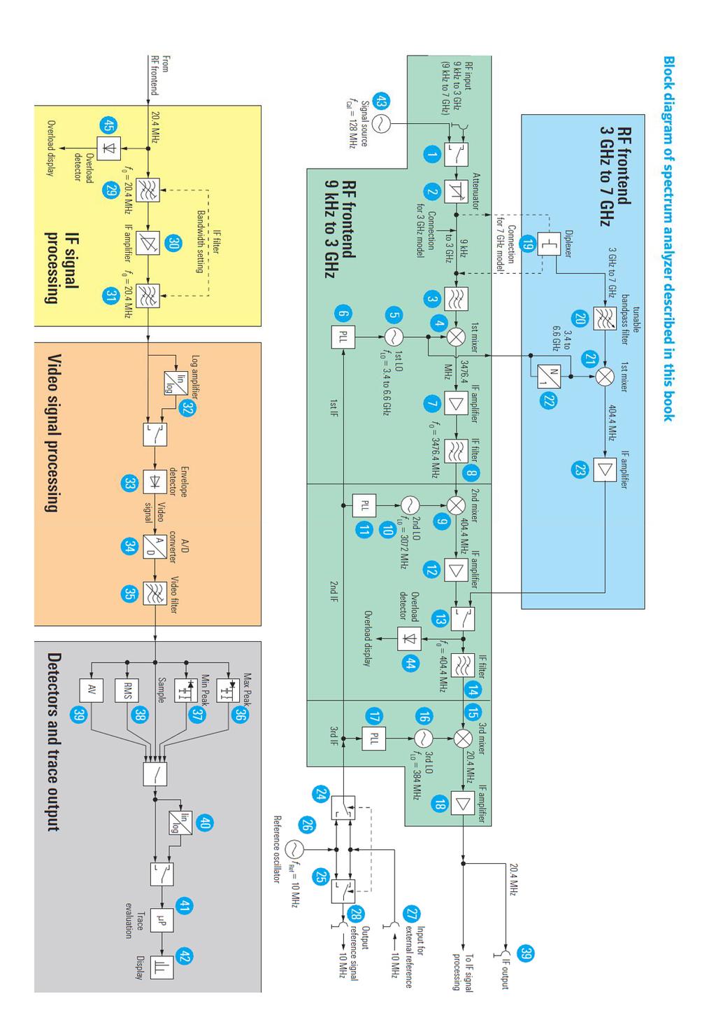
83