Low Frequency Antenna Locator
|
|
|
- Aldous Douglas
- 6 years ago
- Views:
Transcription
1 Project Number: ECE-DC-0801 Low Frequency Antenna Locator A Major Qualifying Project Report: submitted to the Faculty of the WORCESTER POLYTECHNIC INSTITUTE in partial fulfillment of the requirements for the Degree of Bachelor of Science by Brian Janice Matthew Lowe Scott Steinmetz Date: April 30, 2009 Approved: Professor David Cyganski, Advisor Professor Arthur C. Heinricher, Co-Advisor
2 Abstract It is important to be able to find the position of a sensor remotely from a collection of receive signals indoors and outdoors. This is useful when tracking a person s location indoors. The use of GPS is inadequate when used inside. A closed form expression of the integral related to the coupling between two small loop antennas in the near and far fields has been derived. The inverse problem is then solved to locate a transmitter given arbitrary orientation and position based on a received signal. Due to the size of the problem, Maple has been used to assist various computations and simplifications. Two successful approaches to the inverse problem are proposed and tested - one using Procrustes method and one using a self-developed determinant method - providing a complete proof of concept. ii
3 Acknowledgments We would like to thank Professor Cyganski for his great intuition and insight which helped guide us through this project. Also, we would like to thank Professor Heinricher for always challenging us to believe in our work. Finally, we would like to thank Vivek Varshney for providing us with the data he collected for his thesis along the foundation he built concerning the Procrustes searching algorithm. iii
4 Executive Summary It is very helpful to be able to locate and track a sensor based on external received data. One example of this is the case of locating a firefighter as he or she moves throughout a building. The use of Global Positioning System (GPS) is not applicable when trying to track a sensor inside most buildings. This is because high frequency signals are easily reflected off of walls and metal obstacles such as appliances. This Major Qualifying Project (MQP) obtained a general expression describing the coupling between two antennas in the near and far fields. The fields used for this project describe the electromagnetic fields of a small loop antenna. They are shown below. ( 1 E φ = 30β 3 dm H r = β3 dm 2π H θ = β3 dm 4π E θ = E r = H φ = 0 βr ( j (βr) (βr) 3 ( 1 βr j ) (βr) 2 sin θ e jβr ) cos θ e jβr j (βr) 2 1 (βr) 3 ) sin θ e jβr (0.0.1) 1 The terms which are proportional to represent the strict near field. Those which are (βr) 3 proportional to 1 βr correspond to the strict far field. These fields are used in deriving the closed form analytic expression. The integral which needs to be evaluated is shown below. S [E B H A E A H B ] n ds (0.0.2) E A, E B, H A, and H B correspond to the electromagnetic field vectors for two antennas, A and B, as given in the field equations seen in Equation The first step in solving this problem is to define its geometry. The fields describe an antenna pointed vertically. This means that the array of rotation angles (α 1, α 2, α 3 ) must be used to describe an antenna which is already oriented at those angles and must be rotated back to point in the z-direction. This construction of the geometry allowed for various techniques to be applied in deriving a closed form expression of Equation The geometry is visually shown in Figures 1 and 2. iv
5 Figure 1: Spherical Coordinate System Figure 1 shows the angle definitions for representing points in spherical coordinates. Figure 2: Orientation Angles v
6 The integral was then solved using the following approach. 1. Consider antenna A located at the origin oriented in the z direction 2. Place antenna B at an arbitrary point (r 0, θ 0, φ 0 ) with orientation (α 1, α 2, α 3 ) 3. Unrotate antenna B s electromagnetic fields by the negative angles ( α 1, α 2, α 3 ) 4. Construct the surface on which to integrate the fields. These steps required mathematical tricks involving the use of limit properties and using the problem s geometry to apply a useful series representation. Once this closed form expression was derived, it needed to be tested to ensure that is was correct. This relied heavily on analyzing the geometry to find cases of symmetries. These cases include symmetries about axes along with transformational symmetries due to rotations. The phase and amplitude of the expression was used to test these scenarios. One interesting and insightful result shows the near and far field behavior of the phase. The phase remains constant in the strictly near field case and behaves as expected in the far field, as seen in Figure 3. Figure 3: Phase Behavior in the Near and Far Fields Once the closed form expression was thoroughly tested, the inverse problem was considered. This inverse problem used the analytic solution to design a method to locate a transmitters position based on a received signal. A brute force approach is infeasible as it is a 6-dimensional problem. Two methods were created in order to reduce the dimensionality of the problem and provided a solution. In each method, the transmitter was placed somewhere in a 10 by 10 grid with nontrivial orientation and one receive antenna was placed on each of the four corners. These methods both utilized the formation of a coupling matrix. This coupling matrix is defined in Equation c xx c xy c xz CM = c yx c yy c yz (0.0.3) c zx c zy c zz vi
7 The elements c represent the coupling between the corresponding axes of two antenna triplets at points A and B, composed of three orthogonal loop antennas. The first approach of solving the location problem took advantage of a Procrustes-based solution. This involved searching a grid for the minimal error of a rotation of the coupling matrix into an expected coupling matrix at each point. The scenario in which the transmitter was located at (7,7) with four receive antennas located at (0,0), (10,0), (10,10), and (0,10) is shown in Figure 4. Figure 4: Problem Layout The results from this solution are seen in Figure 5 below. Figure 5: Procrustes Approach The second method utilized the fact that the determinant of the coupling matrix is invariant under rotations of the transmitter. This gives powerful information regarding the radial position of the transmitter without knowing the rotation or orientation of the transmitter. Given the vii
8 same layout described above, this method produces the result seen in Figure 6. Figure 6: Determinant Approach This solution provided an accurate estimation of the location of the transmitter. This method was faster than the Procrustes Method but required multiple receive antennas; however, the enhanced Procrustes Method worked well with only one receive antenna. This MQP met the first goal of deriving a general analytic expression describing the coupling between two small loop antennas. Additionally, the project met its other goal of solving the inverse problem of locating a transmitter given a received signal. Two valid approaches for this second problem were designed and tested. There are various topics to consider for future development. First, the algorithms used in both design approaches may be optimized. One potential adaption involves a hybrid method which utilizes the Determinant Method to narrow the region of searching for the Procrustes Method and may result in a faster, more accurate solution. Another topic to consider is the problem of deciding where to optimally place the receive antennas. Also, more research may be conducted regarding the properties of the coupling matrix and the detailed behavior of the coupling expression in the near field. Finally, this project provided a concrete proof of concept for the solution to this problem offering the potential for a physical implementation of this theory to be created, tested, and patented. viii
9 Contents Abstract ii Acknowledgments iii Executive Summary iv 1 Introduction Problem Statement Antenna Background Precision Personnel Locator and The Mantenna Problem Approach Analysis Geometry Coupling Expression Field Rotation Surface of Integration Integration Maple Testing Solution Amplitude Phase Symmetries Coupling Between Modes Phase Information Design Design Intro Coupling Matrix Properties of the Coupling Matrix Procrustes Problem Procrustes Problem Approach Results Enhanced Procrustes Problem Approach Determinant Method Approach Results Conclusions Analysis Design Future Development Bibliography 34 ix
10 6 Maple Worksheets Amplitude Analytic Solve Basic Definitions Determinant Field Ellipses Integrals Phase Power Procrustes Problem Procrustes Problem Rotation Demo x
11 List of Figures 1 Spherical Coordinate System v 2 Orientation Angles v 3 Phase Behavior in the Near and Far Fields vi 4 Problem Layout vii 5 Procrustes Approach vii 6 Determinant Approach viii 7 Geometry Geometry Second Antenna Parallel and above The First Antenna Two Antennas Side-by-Side Log-Log Plot of Amplitude vs. Distance Second Antenna Revolving Horizontally Amplitude Plot of Horizontal Revolution Fields Entering from Top-to-Bottom Amplitude Plot of Vertical Revolution Second Antenna Halfway through Rotation Amplitude Plot of Rotation Plot of Phase vs. Distance Phase Plot of Horizontal Revolution Phase Plot of Vertical Revolution Phase Plot of Rotation Error for antenna K Error for antenna L Error for antenna M Error for antenna N Sum of errors from K, L, M, and N Error for antenna K Error for antenna L Error for antenna M Error for antenna N Sum of errors from K, L, M, and N Determinant Method Locating Transmitter at (7,7) Error from the First Antenna Error from the Second Antenna Error from the Third Antenna Error from the Fourth Antenna Determinant Method Locating Transmitter at (5,7) xi
12 1 Introduction 1.1 Problem Statement In many applications, it is useful to be able to determine the location and orientation of a sensor remotely from a collection of receive antennas. One example of this scenario is the case in which a firefighter s location is to be tracked as he or she explores the interior of a building. The use of Global Positioning System (GPS) will not work for tracking inside most buildings. This project aims to offer a solution to this problem by first deriving an analytic expression describing the general (both near and far field) coupling between two antennas. This solution should be valid for antennas of any arbitrary location and orientation. The second goal of this project is to solve the inverse problem of locating an antenna given the coupling between two antennas. 1.2 Antenna Background An antenna is a common transducer whose purpose is to transmit and receive electromagnetic waves. A transmitting antenna converts a change in electrical current into electromagnetic waves while a receiving antenna converts change in electromagnetic waves into electrical current. When one antenna is brought into the electromagnetic field of another antenna, an effect known as coupling occurs. The coupling between two antennas is described by the power transferred from one to the other. This project will consider the coupling effects between two antennas using a sinusoidally excited circular current loop model for each antenna. This model assumes a theoretical loop antenna with an infinitesimal current source. The small loop antenna creates an electromagnetic field component with terms proportional to 1 βr and 1. It also creates magnetic field components which are proportional to 1 (βr) 2 βr, 1, (βr) 2 1 and. The terms proportional to 1 (βr) 3 βr are commonly known as the far field components. These components consist of both the electric and magnetic fields. The terms which are proportional to are known as the induction terms, or the radiating near field. The terms 1 1 (βr) 2 (βr) 3 are commonly denoted as the reactive near field, or electrostatic field terms. This 1 (βr) 3 is only produced by the magnetic field. In many applications involving high-frequency and/or long distances, these last two terms drop off very quickly and may be neglected. However, this paper will be very concerned with this near field range. When working with low frequencies, the wavelength of an electromagnetic field (λ = c/f) becomes longer, making it less prone to reflections off nearby obstacles. For this reason, this document is mainly concerned with low frequency electromagnetic fields (f = 170kHz) and their behavior within one wavelength from the source. Because the field generated by a low frequency source will reflect less off obstacles, precision indoor location applications where GPS is inadequate may be considered. The near field s behavior is not commonly considered in electrical engineering, as most electromagnetics problems assume that the frame of reference is in the far field. In the far field, the phase of the electromagnetic field varies linearly and is unidirectional. This is not the case when considering the near field, as the phase oscillates nonlinearly along the edge of polarization ellipses. Another factor which far field approximations use is that the Poynting vector, E H, is in the same direction of the unit vector e r and normal to both E and H. In the near field, this is not necessarily the case, however this project deals with a loop antenna which has this property in its near field. Also, in the near field, the Poynting vector decays as 1/R 6 and approaches 1/R 2 when moving into the far field (R is the distance from the radiating 1 term
13 source). Finally, in the far field, the phase of E and H varies linearly with R while is does not in the far field. It is because of these nonlinearities and unusual behaviors that most engineers and scientists do not consider the near electromagnetic field for applications. 1.3 Precision Personnel Locator and The Mantenna The Precision Personnel Locator (PPL) is an ongoing project being developed by WPI. The goal of this project is to create a system to locate and track personnel indoors and outdoors. The PPL utilizes Ultra High Frequency (UHF) in the far field to track movement. Unlike the PPL, the Mantenna operates by homing in on stranded personnel indoors and outdoors instead of tracking. The Mantenna relies on the use of low frequencies in the near field. These projects are being funded by the National Institute of Justice (NIJ) of the US Department of Justice and the Federal Emergency Management Agency (FEMA) of the US Department of Homeland Security (DHS). This project will essentially be a hybrid of these two approaches; utilizing low frequencies in the near field as a method to locate and track personnel 1.4 Problem Approach The coupling expression between two antennas is derived from the following integral 1 ; E A, H A, E B, and H B are the electric and magnetic vector fields for two antennas A and B respectively. [E B H A E A H B ] n ds S This expression is directly proportional to the transimpedance of the two port network composed of antennas A and B. We may find this transimpedance by simply scaling the expression above by the reciprocal of the currents (I A I B ) 1 in each antenna. These currents are representative of those used to generate the electromagnetic fields in antennas A and B not the current induced in one by the other. Although we keep this in mind, we are not concerned with the physicality of the network and thus will disregard this term, as the currents are just a scale factor. The power coupling may also be expressed through this integral as well by taking the magnitude squared of the integral and multiplying by a constant depending on the power radiated by both antennas. Although this is not necessarily what we are interested in, we can see that the integral above is something which we can measure in a real system. This means that if we are to obtain a closed form expression for the integral, we will be able use the data from a receiving antenna to solve for the position of a transmitter in an arbitrary place. This strategy may be enhanced by constructing two antenna units, each composed of three antennas pointed orthogonal to each other. We may then solve for the coupling between each axis of the two units. Once these couplings are solved, we can place the results in a matrix and use the data to better solve for the location of a transmitter. Although this problem seems to be simple once the integral is evaluated, the inverse problem of solving for the position of a transmitter is a six-dimensional problem. Thus we will need to use some close observations along with some results pertaining to linear algebra to solve the problem. 1 Pace, J. Asymptotic Formulas for Coupling between Two Antennas in the Fresnel Region 2
14 2 Analysis 2.1 Geometry Deriving the analytical coupling between two antennas in three dimensions requires a thorough knowledge of the system s geometry. At this point it is crucial to mention that the electromagnetic fields used throughout this paper pertain to a small loop antenna centered on the origin pointing vertically (i.e. current flowing counter-clockwise in the xy-plane). Figure 7 portrays the basic configuration of our loop antenna. Figure 7: Geometry The first thing we should observe is that a system of two arbitrarily oriented elements in 3-space may be generated by holding one in a static condition while translating/rotating the other. We are able to do this because the loop antennas we are dealing with are considered infinitesimally small and symmetric about all axes. Once we have the understanding that we may position one antenna fixed at the origin, we can describe the relative orientations and positions of the remote antenna through 6 dimensions. These include the spherical coordinate triplet (r, θ, φ) and the rotation angles (α 1, α 2, α 3 ). These angles describe counterclockwise rotations about the x, y, and z-axes, allowing us to rotate the remote antenna in any fashion necessary. A picture of this scenario may be seen below in Figure 8 We must take care in understanding the angles describing the orientation of the remote antenna. Recall that fields we are using describe an antenna pointed vertically. This means that the triplet (α 1, α 2, α 3 ) must be used to describe an antenna which is already oriented at those angles and must be rotated back to point in the z-direction. The approach we will be using for deriving the coupling expression may be summarized in the following way: 1. Consider antenna A located at the origin oriented in the z direction 2. Place antenna B at an arbitrary point (r 0, θ 0, φ 0 ) with orientation (α 1, α 2, α 3 ) 3
15 Figure 8: Geometry 3. Unrotate antenna B s electromagnetic fields by the negative angles ( α 1, α 2, α 3 ) 4. Construct the surface on which to integrate the fields. Once we have set up the problem in this manner, we may solve the integral to obtain the analytical expression for the coupling between the two antennas as in the next section. 2.2 Coupling Expression The problem posed in this project pertains to the location of a radiating source in its near electromagnetic field or near field. The separation between near and far electromagnetic fields of a radiating source is ambiguous, thus we will describe it in this section as follows: Near Field: The region of an electromagnetic field where terms of order two and three pertaining to a scaled distance from the source are much larger than those pertaining to unity orders of distance (i.e. 1/(βr) 3 1/(βr) 2 1/(βr), where r is the distance from a source). The term β is crucial to the understanding of the regions of an electromagnetic field. β, called the wavenumber, is inversely proportional to the wavelength of the electromagnetic field. This means lower frequencies that generate longer wavelengths will result in the electromagnetic near field extending farther than a field with a higher frequency. With this definition, we will define the electromagnetic fields pertaining to loop antennas in the near field as described in Strauss 2 : 2 Strauss, I. Near and Far Fields From Statics to Radiation 4
16 ( 1 E φ = 30β 3 dm H r = β3 dm 2π H θ = β3 dm 4π E θ = E r = H φ = 0 βr ( j (βr) (βr) 3 ( 1 βr j ) (βr) 2 sin θ e jβr ) cos θ e jβr j (βr) 2 1 (βr) 3 ) sin θ e jβr (2.2.1) The approach we have used to locate a transmitter in the near field requires us to find a closed form expression of the following integral 3 over the fields generated by two antennas located at arbitrary points A and B: S [E B H A E A H B ] n ds (2.2.2) This may be evaluated using an arbitrary surface around point B with unit normal surface element vector n ds. We have chosen to work in the spherical coordinate system as it is easiest to describe the fields in this fashion. At this time, we will also define our surface of integration as a sphere around the point B Field Rotation This problem requires that the integral be solved for two arbitrarily oriented antennas; to do this, we consider antenna A to be located at the origin and describe the radial and angular displacements of the pair with respect to the antenna at point B alone. This may be done by transforming the vectors E B (r) and H B (r) by rotation matrices. The easiest way we have found to perform this transformation is to reproduce the vectors E B and H B with the standard Cartesian unit vectors. These new representations of the fields will be denoted ẼB(r) and H B (r). The following change of variables is used to express ẼB(r) and H B (r): e r = cos φ sin θe x + sin φ sin θe y + cos θe z e φ = sin φe x + cos φe y (2.2.3) e θ = cos φ sin θe x + sin φ sin θe y sin θe z Taking these new vectors, we assume they are rotated by an arbitrary array of angles, α = (α 1, α 2, α 3 );This implies: Ẽ B (r, α) = R 1 (α)ẽb(r) In other words, the E field produced by an antenna with arbitrary position and orientation is equivalent to an antenna with position r unrotated by the set of angles α 1, α 2, and α 3 about 3 Pace, J. Asymptotic Formulas for Coupling between Two Antennas in the Fresnel Region 5
17 the x, y, and z axes. The following rotation matrix was used for this calculation: R 1 (α) = R 1 z (α 1 )R 1 y (α 2 )R 1 x (α 3 ) R x (α 1 ) = 0 cos α 1 sin α 1 0 sin α 1 cos α 1 cos α 2 0 sin α 2 R y (α 2 ) = sin α 2 0 cos α 2 cos α 3 sin α 3 0 R z (α 3 ) = sin α 3 cos α (2.2.4) It should be noted that when we left-multiply a vector by a matrix, the result will be each component of the original vector times its respective unit vector left-multiplied by the matrix. Since our unit vectors in spherical coordinates are linear combinations of the Cartesian unit vectors, we need only apply these inverse matrices to the unit vectors dependent on r, described in Equation R 1 (α)e r = e r (α) Similarly, we obtain the unit vectors e φ (α) and e θ (α). Applying these new unit vectors to the expressions for E and H, we obtain the same fields rotated by the angles α 1, α 2, and α 3 about the x, y, and z-axes respectively Surface of Integration After rotating the vector fields at point B, we must describe an arbitrary point of the surface of integration. This point will be described as another polar expression with Cartesian bases. First, we will describe the point on the surface of a sphere centered on (x 0, y 0, z 0 ). This defines the surface with respect to antenna A, S A ; S A denotes the boundary of the sphere centered at point B=(x 0, y 0, z 0 ) with respect to point A with radius ε. S A = s A = (x 0, y 0, z 0 ) + ε(cos ϕ sin ϑ, sin ϕ sin ϑ, cos ϑ) = (x 0 + ε cos ϕ sin ϑ, y 0 + ε sin ϕ sin ϑ, z 0 + ε cos ϑ) (2.2.5) Note that the point (r, θ, φ) (ε, ϑ, ϕ). The next step is to describe the same point with respect to the antenna at point B. This point is a bit different since we have antenna B centered on the point (x 0, y 0, z 0 ). We may define a point on the sphere around B in the same way as in substituting x 0 = y 0 = z 0 = 0 S B = s B = (ε cos ϕ sin ϑ, ε sin ϕ sin ϑ, ε cos ϑ) (2.2.6) The normal vector n in Equation may also be written after dividing by the radius of the sphere in Equation n = (cos ϕ sin ϑ, sin ϕ sin ϑ, cos ϑ) Now that we have obtained expressions for the surface, we must transform our coordinates (r, θ, φ) to (ε, ϑ, ϕ). For antenna A, we may just use the spherical coordinates transform on the vector describing S A. That is, 6
18 r A = s A φ A = tan 1 ( sa2 s A1 θ A = cos 1 ( sa3 s A ) ) (2.2.7) Antenna B has a smaller expression for the surface of integration, but the change of variables from r to r B is a bit more complicated. Due to our rotation of the Cartesian basis by α, we must rotate our location of the point on the surface back to where it was before we rotated it. This means we apply the rotation matrix R(α) to the vector s B, and then proceed as in Equation s B (α) = R(α)s B r B = s B (α) ( ) φ B = tan 1 sb2 (α) s B1 (α) ( ) θ B = cos 1 sb3 (α) s B (α) (2.2.8) Now we are able to construct the fields ẼA, H A, ẼB, and H B in terms of (ε, ϑ, ϕ, α 1, α 2, α 3 ) by substituting their respective coordinate transforms Integration The only thing left to do is plug the fields into Equation and integrate over the sphere using ds = ε 2 sin ϑdϑ dϕ as the surface element. This is the Jacobian of the change of variables from Cartesian to spherical coordinates. 2π π 0 0 [ẼB H A ẼA H B ] n (ε 2 sin ϑ dϑ dϕ) (2.2.9) Now we will return the notion that the surface of integration may be arbitrary. This implies that the result of the integral is unaffected by the radius of the sphere which we choose. For example, one may consider the surface to be a hemisphere with infinite radius and integrate over a plane separating antennas A and B. This surface does not offer many advantages; however, the sphere with arbitrarily small radius centered on point B will produce the same expression. That is, if we take the surface around antenna B to be a sphere with radius ε approaching 0, we may express Equation under a limit with hopes of a simpler result in the following way lim ε 0 2π π 0 0 [ẼB H A ẼA H B ] n (ε 2 sin ϑ dϑ dϕ) (2.2.10) Another simplification which can be made at this point is to transform the location of antenna B at point (x 0, y 0, z 0 ) into a spherical representation of terms (r 0, θ 0, φ 0 ). This will 7
19 eliminate some square roots and other transcendental functions which may be unfriendly to integrate. This requires a change of variables x 0 = r 0 cos φ 0 sin θ 0 y 0 = r 0 sin φ 0 sin θ 0 (2.2.11) z 0 = r 0 cos θ 0 Finding the antiderivative, evaluating the integral, and taking the limit is all that is left for deriving the expression we wish to have. This integral has an incredible number of terms and would be impractical to solve by hand. This is because we have multiplied the unit vectors used to express the field at point B with three matrices and took two cross products. We also had to perform a change of variables in which we multiplied a point on a sphere by three matrices in Cartesian coordinates. After these operations are performed, the expression is unmanageable by hand. A numerical result for this could be easily computed, but our goal is to determine a full analytical expression; it is because of this that to turn to Maple Maple Although Maple is capable of handling large symbolic expressions with ease, Equation was still too large for Maple to evaluate. Because of this, we had to use some techniques which were not quite obvious at first. The first simplification was to pass the limit through the integral since ε is not a variable of integration. This resulted in a dead end because of the shear number of terms of the integrand; the limit of such an expression could not be evaluated by Maple. Once passing the limit through the integral failed, the idea of expanding the integrand of Equation into a Maclauren series and taking the leading term independent of ε was proposed. Once this was done, the integrand was largely simplified. Maple was still unable to evaluate the expression even with this simplification. It should be noted that the original expression of the integrand of Equation contains the addition of two extremely large ratios. After taking the constant term of the Maclauren series, the integrand became the addition of 200 terms. This allowed us to break the integral into 200 simpler integrals and tell Maple to integrate them one by one. Many of these 200 terms vanish after integration, and once we evaluated this expression, we obtained the result 8
20 which we had been looking for c zz = 30β 4 dm 2 e jβr [ j βr ( cos α1 sin α 2 sin α 3 sin θ cos θ sin φ + cos α 2 cos α 1 cos 2 θ+ cos α 3 cos α 1 sin α 2 sin θ cos φ cos θ sin α 1 cos α 3 sin θ cos θ sin φ+ sin α 1 sin α 3 sin θ cos φ cos θ cos α 2 cos α 1 ) + 1 (βr) 2 (3 cos α 3 cos α 1 sin α 2 sin θ cos φ cos θ + 3 sin α 1 sin α 3 sin θ cos φ cos θ+ 3 cos α 1 sin α 2 sin α 3 sin θ cos θ sin φ + 3 cos α 2 cos α 1 cos 2 θ cos α 2 cos α 1 3 sin α 1 cos α 3 sin θ cos θ sin φ) + j (βr) 3 (3 cos α 3 cos α 1 sin α 2 sin θ cos φ cos θ + 3 sin α 1 sin α 3 sin θ cos φ cos θ+ 3 cos α 1 sin α 2 sin α 3 sin θ cos θ sin φ + cos α 2 cos α 1 cos 2 θ ] cos α 2 cos α 1 3 sin α 1 cos α 3 sin θ cos θ sin φ) (2.2.12) 9
21 2.3 Testing Solution Throughout the duration of this project, two expressions for were found and shown to be incorrect. Once an expression is obtained, the next step is to create tests to ensure that it is correct. This process relies heavily on physical symmetries about axes and transformational symmetries due to rotations. Another useful technique is considering various asymptotic and limiting cases to ensure appropriate behavior in the strictly near and far fields. This step is very important because the first two solutions obtained were found to exhibited incorrect behavior in certain cases. The expression derived above behaves as expected in all cases which were constructed. The following displays some of the more prominent and interesting cases Amplitude The first case to consider involves observing the limiting and asymptotic behavior of the amplitude as the antennas move towards and away from one another. In the near field, the amplitude is larger when antenna B is above antenna A compared to when antennas A and B are side-byside. However, in the far field, this amplitude should be zero when the antennas are aligned on top of one another and should dominate when they are side-by-side. These configurations are shown in Figure 9 and Figure 10 with results shown in Figure 11. Figure 9: Second Antenna Parallel and above The First Antenna 10
 dominates and the Figure 9 coupling tends to 0. This agrees with the expected behavior.")
22 Figure 10: Two Antennas Side-by-Side Note that this plot is a log-log plot. As r tends to zero, the plot of the Figure 9 coupling (red) dominates. However, as r becomes large, the Figure 10 coupling (green) dominates and the Figure 9 coupling tends to 0. This agrees with the expected behavior. In an effort to inspect the symmetries with respect to rotations, the case of antenna B positioned at θ = π/2 at a distance of λ/40 where λ is the wavelength of the transmitted signal. This distance is well within the near field is considered while revolving the antenna around the origin, from φ = 0 to 2π. Based on the geometry of the situation, the amplitude should remain constant throughout the revolution. The configuration of this case is shown in Figure 12. This configuration does exhibit the expected behavior. This may be seen in Figure

23 Figure 11: Log-Log Plot of Amplitude vs. Distance Figure 12: Second Antenna Revolving Horizontally 12
, the coupling is maximized.")
24 Figure 13: Amplitude Plot of Horizontal Revolution A more interesting configuration consists of antenna B in the near field (λ/40) with φ = 0 and it revolving around antenna A from θ = 0 to π. This involves the antennas moving from Figure 9 to the position in Figure 14. Figure 14: Fields Entering from Top-to-Bottom As this test begins (θ = 0), the coupling is maximized. The antenna revolves about the origin and the coupling begins to decrease in amplitude. Then the field lines become tangential to the revolving loop, there is no coupling (zero amplitude). The amplitude begins to increase again as the antenna moves into the position seen in Figure 14. When the two antennas are aligned side-by-side (θ = π/2), it reaches another localized maximum. The pattern follows clearly as the angle moves from π/2 to π. Note that the angle at which this zero amplitude occurs is dependent on the r chosen. This result is seen to follow the expected behavior in Figure 15. Another case to test involves inspection of the symmetries due to rotations. This case places 13

25 Figure 15: Amplitude Plot of Vertical Revolution the two antennas aligned one above the other (θ = φ = 0) in the near field (λ/40). The angle α 2 is then increased from 0 to 2π. This results in the second antenna rotating in place above the first antenna. The configuration starts at Figure 9 where it has maximum amplitude, then its amplitude begins to decrease as it starts to rotate, and then reaches Figure 16 at π/2 where it has zero coupling. Due to the symmetry, the pattern then will reverse as the antenna move from α 2 = π/2 to π. Figure 16: Second Antenna Halfway through Rotation The result in Figure 17 shows that the solution behaves as expected in this case. 14
26 Figure 17: Amplitude Plot of Rotation Phase The phase is used to test the solution and ensure correct results in the near field and far field. As antennas move away from one another, one expects to see a periodic linearly decreasing phase. In the far field, the phase should follow the periodic behavior of continuously dropping from π to π and then experience a jump from π back to π. On the other hand, the phase should remain constant as the antennas move radially in the near field. Figure 18 shows the results found from testing this case of the solution in Maple. This configuration of the antennas is displayed in Figure 10. This plot shows that the phase remains relatively constant until about λ/9. This corresponds to about 150m in Figure 18 with β = and dm = 1. The phase then smoothly makes its way into the expected far field behavior. This transitional period is when the antenna is beginning to approach its far field behavior. The phase attains strictly far field behavior at approximately one wavelength. Next, the solution is tested in the limiting case with the antenna in the near field (λ/40) and the antenna positioned at θ = π/2. This places the antenna in the xy-plane. The antenna then revolves around the origin by increasing φ from 0 to 2π. This configuration is shown in Figure 12. The phase should remain constant throughout this motion. The resulting behavior is exhibited in Figure 19 with the phase remaining at π/2 throughout the revolution. 15
27 Figure 18: Plot of Phase vs. Distance Figure 19: Phase Plot of Horizontal Revolution 16
28 Another interesting situation in the near field (λ/40) is when φ is fixed to 0 and θ is varied from 0 to π. This configuration is seen in Figure 12 and the result is shown in Figure 20. The phase starts off at π/2, then switches to π/2, and returns to π/2. The values of positive and negative π/2 correspond to the fields exciting the antenna through the bottom and from the top. The angle at which this transfer in sign of the phase occurs depending on the radial distance from the antenna at the origin. Figure 20: Phase Plot of Vertical Revolution Note that the spikes in the plot at the corners of jumps are due to numerical interpolation errors. In order to ensure the solution exhibits appropriate symmetries due to rotations, it is tested in the case where θ and φ are 0 and the antennas are in the near field (λ/40). The arbitrarily oriented antenna is rotated in place as we vary α 2 from 0 to 2π. As the antenna rotates just beyond vertical as seen in Figure 10, the phase should flip in sign. The result is seen in Figure 21 below. 17
29 Figure 21: Phase Plot of Rotation As α 3 goes just beyond π/2, the antenna rotates just beyond vertical and the fields enter from the top causing a flip in phase. As the angle passes 3π/2, the fields begin to pass through the bottom again and the phase returns to π/ Symmetries Once the magnitude falloff and phase information were shown to behave properly, symmetries of the same cases are expected to provide the same results. This may be done by considering antennas pointed along axes different than z and rotating along the corresponding angles. For example, if we are to rotate Figure 9 and Figure degrees clockwise (both antennas facing along the x-axis with antenna B moving along the x-axis/z-axis), we obtain the same results shown in Figure 11 as expected. Another example using Figure 12 may be constructed by rotating the figure 90 degrees clockwise. In this case, we rotate the antenna about θ instead of φ and obtain the same constant phase plot. The convention used for equivalent scenarios is shown below. 1. Initial orientation along x-axis (a) Translate along x-axis. (b) Revolve about θ with initial φ = π/2. 2. Initial orientation along y-axis (a) Translate along y-axis. (b) Revolve about θ with initial φ = Initial orientation along z-axis (a) Translate along z-axis as in Figure 9. 18
30 (b) Revolve about φ with initial θ = π/2 as in Figure 12. The scenarios with different initial orientations of antennas A and B may be tested after finding analytical expressions for separate integrals described in Section 3.2. These test cases show that there are no flaws in the solution and that it is in fact the correct analytic solution. The next step is to consider how to apply this solution practically. 2.4 Coupling Between Modes It is clear that the analytical expression for Equation in Equation depends only on the following powers of r: 1/r, 1/r 2, and 1/r 3. This leads us to question if couplings between separate modes (we will call each of the coefficients of 1/r n a separate mode for each n) of electromagnetic fields are independent of each other. That is, if we shut off the 1/r n (n = 1, 2, 3) component of antenna A s fields, will there be a 1/r n in the coupling to antenna B? Furthermore, if we shut off every component of the fields generated by A except coefficients of 1/r n, will the coupling between A and B be dependent on 1/r n alone? The answer to this question is immediately evident after we create modified expressions for the electromagnetic fields in Equation 2.2.1, replacing coefficients of 1/r n with 0 depending on which scenario is being tested. If we find that one of the modes in question is required to generate a 1/r n term in the coupling between A and B, we may say that the coupling is independent of other modes. There are several cases which must be tested to determine this, all of which may be done with Maple. The cases follow the pattern: 1. Reduce the E & H field for one of the antennas to the 1/r component alone (a) Leave E & H field for other antenna alone (b) Reduce E & H field for other antenna to 1/r terms only (c) Reduce E & H field for other antenna to 1/r 2 terms only (d) Reduce E & H field for other antenna to 1/r 3 terms only (e) Reduce E & H field for other antenna to 1/r and 1/r 2 terms only (f) Reduce E & H field for other antenna to 1/r and 1/r 3 terms only (g) Reduce E & H field for other antenna to 1/r 2 and 1/r 3 terms only 2. Reduce the E & H field for one of the antennas to the 1/r 2 component alone. 3. Reduce the E & H field for one of the antennas to the 1/r 3 component alone. 4. Reduce the E & H field for one of the antennas to the 1/r and 1/r 2 components. 5. Reduce the E & H field for one of the antennas to the 1/r and 1/r 3 components. 6. Reduce the E & H field for one of the antennas to the 1/r 2 and 1/r 3 components. 19
31 It is clear that the result for such configurations as 3(d) will be identically 0 due to E r s independence of 1/r 3 ; however, we would like to be sure that the result is false in other nontrivial cases. When solving case 1(a), we find that the coupling has a 1/r 2 in the expression. When solving case 2(a), we find that the coupling has a 1/r 3 in the expression. This answers our question. We can now say that the radial component of coupling between two electromagnetic fields is not determined by the transmitted modes. 2.5 Phase Information Since the coupling between antennas A and B is complex valued, we are naturally interested in the phase variations produced by changes in position and orientation in the near field. To do this, we observe the argument of the coupling expression. We have already seen such plots in Section These plots portray the phase as a periodic discontinuous function jumping from π to π or simply a constant value when changing α, θ, or φ. Although the plot in Figure 18 varies a bit before going into the far field, we can see it behaves as a constant in the near field. Taking these variations into consideration, there is no immediate advantage of using phase information in the near field to locate a transmitter. 20
32 3 Design 3.1 Design Intro Now that we have an analytical solution for the coupling between two loop antennas, we may apply it to the inverse problem of locating a transmitter using its received data. This problem is a sixdimensional search for the parameters (r, φ, θ) and (α 1, α 3, α 3 ). A brute force approach to search for these parameters would be intractable at this point and will be disregarded. In this section, an accurate and efficient solution must be designed to solve the problem at hand. As mentioned in Section 1.4, we may construct two antenna units composed of three loop antennas orthogonal to each other. In other words, we take three loops of current flowing counterclockwise in the xy-plane, the yz-plane, and the xz-plane centered at the origin. This unit may be considered one antenna triplet. The triplet is not necessarily a realizable structure, however the displacement of such antennas from the origin by a small amount will leave the system relatively unaffected as long as the antennas remain orthogonal. When considering two of these triplets, we may solve for more than just the coupling between the antennas pointing in the z direction; in fact, we may solve for the couplings between every pair of antennas found on the triplets located at points A and B (i.e. x-axis coupling to y-axis coupling). These couplings should be generalized as in the z-axis to z-axis case solved in Section 2.2. In the next section, the notion of the coupling matrix will be introduced. 3.2 Coupling Matrix Once the integral from Section 2.2 is solved for two antennas vertically oriented (we will call this case zz coupling), we can solve for the coupling between every case of antennas A and B facing in the x, y, and z directions. This may be done for each case by right-multiplying the rotation matrix R(α) in Equation by R y ( π 2 ) for x coupling or R x( π 2 ) for y coupling. The cases where antenna A is not oriented along the z-axis requires us to left-multiply the fields at point A by R (x or y) ( π 2 ), and to leftmultiply the vector s A from Equation by R (x or y) (± π 2 ) and following the steps of Equation for (y or x) coupling. Thus we generate nine expressions and create a matrix of the couplings: CM = Properties of the Coupling Matrix c xx c xy c xz c yx c yy c yz c zx c zy c zz (3.2.1) In this section, we will observe some properties of the coupling matrix which are interesting. First, we note that each row vector of has magnitude independent of α. In other words, the magnitude of coupling from three orthogonal antennas to a receiver will solely depend on the location of the transmitter and not its orientation. The expressions for each of these magnitudes are as follows c xx 2 + c xy 2 + c xz dm 4 β 6 = ( 1 cos 2 φ + cos 2 φ cos 2 ) θ r 2 ( 1 5 cos 2 φ + 5 cos 2 φ cos 2 ) θ β 2 r 4 ( cos 2 φ 3 cos 2 φ cos 2 ) θ + β 4 r 6 (3.2.2) 21
33 c yx 2 + c yy 2 + c yz dm 4 β 6 = ( cos 2 θ + cos 2 φ cos 2 φ cos 2 ) θ r 6 ( 4 5 cos 2 θ 5 cos 2 φ + 5 cos 2 φ cos 2 ) θ + β 2 r 4 ( 4 3 cos 2 θ 3 cos 2 φ + 3 cos 2 φ cos 2 ) θ + β 4 r 6 (3.2.3) c zx 2 + c zy 2 + c zz dm 4 β 6 = ( 1 cos 2 θ r 2 ) ( 1 5 cos 2 θ β 2 r 4 ) + ( cos 2 ) θ β 4 r 6 (3.2.4) Next, we compute the determinant of Equation This is also invariant on α and may be expressed as follows c xx c xy c xz [ c yx c yy c yz (j β c zx c zy c zz = 303 β 3 dm 6 5 r 5 + 5β 3 r 3 3βr 5jβ 2 r 2 ] ) 5r 9 e 3jβr (3.2.5) Since this expression is independent of α, φ and θ, we may say that the received data from a transmitter is invariant under orthogonal transforms of the coupling matrix. That is, the received data depends solely on the euclidean distance of B from the origin. These equations are valid for the analytical solution for the location of antenna B in polar coordinates. Although we have a theoretical solution for such a problem, the addition of obstacles or noise to the system may affect the equations and cause the answer to be inaccurate. Thus, we will develop a search method which will hopefully take this into account and be used to augment the location problem to ensure greater accuracy. 22
34 3.3 Procrustes Problem One of the proposed searching algorithms for the location problem is an approach to solving Procrustes Problem created by Shinji Umeyama. Procrustes Problem is a linear algebra problem which, given a matrix, seeks the scaling, rotation, and translation of a different matrix to transform it into the initial matrix. In our case, we are hopeful in assuming that the coupling matrix of received data at point A from a triplet at point B (the transmitter) is multiplied by a rotation matrix when the triplet at point B s orientation is varied. This is a simplified version of Procrustes Problem, as we do not require the scaling or translation of the coupling matrix. It will soon be evident that we will not even require the explicit expression for the rotation matrix in this problem. Umeyama s approach to Procrustes Problem is preceded by the following Lemma: where min A P R B 2 = A 2 + B 2 2tr(DS) S = { I if det (AB T ) 0 diag(1, 1,, 1, 1) if det (AB T ) < 0 and UDV T is the singular value decomposition of AB T (UU T =V V T = I, D = diag(d i ), d 1 d 2 d m 0) (3.3.1) This formula is basic in the sense that it tells us the minimum error any rotation matrix P could produce when assuming two different matrices are rotations of one another. If we are to implement such a formula in our problem, it must be determined whether or not the received coupling matrix, CM, is under the affect of a rotation when the triplet at point B is rotated. To do this, we take a numerical result at first to see if there is an approximate behavior to what we are looking for. That is, if CM is not transformed by a pure rotation, it may be transformed by a matrix extremely close to a rotation. Consider the coupling matrix CM as the received data from a transmitter at point B with orientation α 0, and CM ˆ as the data from a transmitter at the same point with orientation α 1. Assuming CM ˆ is a rotation of CM, ˆ CM = P CM ˆ CMCM 1 = P But P is an orthogonal transform, so P P T = I ( ˆ CMCM 1) ( ˆ CMCM 1) T = I (3.3.2) Checking the result of Equation numerically in Maple, we have found that the coupling matrix does not vary under a rotation while the transmitter is oriented differently. In other words, ( CMCM ˆ 1 )( CMCM ˆ 1 ) T I. Before disregarding this approach, we may c heck if either R{CM} or I{CM} are transformed by rotations when the transmitter is oriented differently. For such cases, we see that R{CM} is under the affect of a matrix P extremely close to a rotation, i.e. ( R{ ˆ CM}R{CM} 1) ( R{ ˆ CM}R{CM} 1) T I However, I{CM} does not behave in this fashion. This is because I{CM} R{CM} in the near field, which tells us that variations in near field coupling magnitude are mostly governed by changes in the imaginary part of the coupling. Using this to our advantage, we will attempt to apply our solution to this simplified Procrustes Problem to the real part of the coupling matrix only Procrustes Problem Approach It is not immediately evident how this approach will aid us in locating an antenna at point B. Lemma will aid us in reducing the problem s dimensionality by 3, thus eliminating the variables α 1, α 2, and 23
, with orientation α = 0 for all i points on the grid.")


35 α 3 from the search for point B. This is done by considering a three dimensional grid of the i possible locations (x i, y i, z i ) of point B (larger i would mean more resolution). Once we construct this grid, we may calculate the coupling matrix, CM i (i = 1, 2,...), with orientation α = 0 for all i points on the grid. Once this is done, we consider the coupling data measured at point A, CM R. Using the formula presented in Lemma 3.3.1, we may calculate the minimum error e i required to transform R{CM R } into R{CM i } for all i points on the grid. Once all i errors are calculated, we may find the best approximate point B= (x k, y k, z k ) by taking k corresponding to min {e k}. That is, we take the minimum of all minimal k errors calculated and say that it corresponds approximately to the point B. The use of multiple antennas will also aid in the accuracy of our search since we may take the collective minimum errors, add them together, and find the minimum over all errors added together. Multiple receive antennas provide a more reliable search, as the results for one antenna may be incorrect at a point. Adding the errors of multiple antennas rotations together at all points is assumed to aid in the precision of the location problem, as it is assumed that on average the processed data from each receiver will be mostly correct Results The results for this idea seem to be promising; however since the matrix R{CM} contains such small values, a large number of digits must be used when calculating its determinant and singular value decomposition (the elements are on the order of for point B spaced approximately 13m away from point A with β = and dm = 1); also, RCM stays relatively constant in broad regions of the grid. This is reflected in our results where there are large regions of close errors. The following plots represent the minimum errors (we take log 10 of the errors for better visualization) computed for all points with transmitter point B = (7, 7, 0), α = (0, π 7, π 3 ) and four receiver antennas located at points K = (0, 0), L = (10, 0), M = (10, 10), and N = (0, 10). The subfigure (a) is the error plot for the range (1, 1) (x, y) (9, 9), (b) is the error plot for the range (4, 4) (x, y) (9, 9), and (c) is the surface composed of the errors in plot (b). (a) (b) (c) Figure 22: Error for antenna K 24
")


36 (a) (b) (c) Figure 23: Error for antenna L (a) (b) (c) Figure 24: Error for antenna M (a) (b) (c) Figure 25: Error for antenna N 25

37 (a) (b) (c) Figure 26: Sum of errors from K, L, M, and N 3.4 Enhanced Procrustes Problem Approach We may come up with a better approach at this point using the full information given by both the imaginary and real parts of the coupling matrix. After Umeyama proves Lemma in his paper, he solves for the matrix P that produces the minimum error. This is done with the formula where P = USV T S = { I if det (U) det (V ) = 1 diag(1, 1,, 1, 1) if det (U) det (V ) = 1 and UDV T is the singular value decomposition of AB T (UU T =V V T = I, D = diag(d i ), d 1 d 2 d m 0) (3.4.1) The rotation matrix P may be computed for all points (x i, y i, z i ) in a grid, given the real part of the received coupling data R{CM R }. It may be shown numerically that P resembles the matrix R 1 (α) from Section with a fixed rotation. We say resembles, because P is equivalent to R 1 (α) with the last two elements in the first column and row (r 12(α), r 13(α), r 21(α), r 31(α)) multiplied by 1. This result was found by calculating the real part of the coupling matrix, R{CM R }, for an arbitrary point (x 0, y 0, z 0 ) with fixed α 0, calculating the matrix P for the point along with R 1 (α 0 ) and comparing their values. Once the matrix P is obtained, we may solve for α 0 by finding the rotations corresponding to the expression min α R 1 (α) P F where F denotes the Frobenius Norm ( ) 1/2 m,n f ij 2 for an m n matrix, F i,j=1 (3.4.2) After solving for α, we may substitute it into the analytic, complex valued, coupling matrix CM i evaluated at (x i, y i, z i ). Once we have computed CM i, we calculate the error at point i e i = CM i CM R F Calculating e i for all i points on a search grid, we may find the best approximate to point B=(x k, y k, z k ) by taking k corresponding to min {e k}. That is, we take the minimum of all errors calculated and say k that it corresponds approximately to the point B. The following plots represent the minimum errors (we take log 10 of the errors for better visualization) computed for all points with transmitter point B = (7, 7, 0), α = (0, π 7, π 3 ) and four receiver antennas 26
.")
 (9, 9), (b) is the surface composed of the errors")


38 located at points K = (0, 0), L = (10, 0), M = (10, 10), and N = (0, 10). The subfigure (a) is the error plot for the range (1, 1) (x, y) (9, 9), (b) is the surface composed of the errors with the range (4, 4) (x, y) (9, 9). These plots are very accurate and the contours are concentrated directly on (7,7). However, this approach takes signifacantly longer than the original Procrustes Method. (a) (b) Figure 27: Error for antenna K (a) (b) Figure 28: Error for antenna L 27


39 (a) (b) Figure 29: Error for antenna M (a) (b) Figure 30: Error for antenna N (a) (b) Figure 31: Sum of errors from K, L, M, and N 28
40 3.5 Determinant Method This design method was self-developed for this project. Similar to the Procrustes Method, it utilizes a grid-search approach. However, this method relies on the coupling matrix s property of the determinant being invariant under rotations of the transmitter. This allows for easy access to the radial location of the transmitter without knowing its orientation. The limitation of only knowing radial information from the receive signal is overcome by using multiple receive antennas Approach This approach uses the same basic simulation layout discussed in Section 3.3. The i th given received signal, R i, is defined in Equation R i = CM r= (xt x i) 2 +(yt y i) 2, θ= π 2, φ=arctan yt y i xt x i, α 1=α 1t, α 2=α 2t, α 3=α 3t (3.5.1) The grid-search approach requires finding the coupling between the i th antenna and a particular point on the grid. This coupling is called M i and is defined in Equation M i (x, y) = CM r= (x x i) 2 +(y y i) 2, θ= π 2, φ=arctan y y i x x i, α 1=0, α 2=0, α 3=0 (3.5.2) The procedure to find the error at a given point (x j, y j ) in the search grid according to the i th receiver is shown in Equation (det (M i (x j, y j )) det (R i )) 2 E i (x j, y j ) = (3.5.3) det (R i ) By using this procedure at each point on the search grid this method finds the difference between det(m i ) and det(r i ) which will be zero if the correct location is scanned or if the position lies on the boundary of the sphere going through the transmitter s location which is centered about the receive antenna. The result is then normalized by dividing by det(r i ). The necessity of this normalization will be more clear as multiple receive antennas are considered. As alluded to above, this method only gives information describing the radial distance between the two antennas. Therefore, the method gives the boundary of the sphere on which the transmitter lies. Using this method with multiple receive antennas allows for the position to be triangulated appropriately by summing the errors. The normalization factor in Equation is needed to ensure that the error from receive antennas which are closer to the transmitter are not overpowering the receive signals from antennas which are more distant. This method appears to be promising but it must be tested for accuracy and performance. 29
, (10,0), (10,10), and (0,10).")

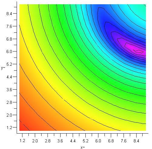
 shows a contour plot of the error with both x and y varying from 1 to 9; (b) shows a contour plot of the error with both x and y varying from 4 to 9; (c) shows a")
 (b) (c) Figure 32: Determinant Method Locating Transmitter at (7,7) The results in Figure 3.5.2 show the error which is seen when the log of each antenna s error is summed.")
 is on the order of 10 42 times larger than the error at the transmitter s actual location, (7,7).")
41 3.5.2 Results One of the major conveniences with this method is the fact that it is very easily implemented in Maple. The code for this implementation is located in the Appendix. The case of interest involves a 10 by 10 grid located in the first quadrant of the xy-plane with one receiver located at each corner of the grid: (0,0), (10,0), (10,10), and (0,10). The transmitter has been positioned at (7,7) with a nontrivial orientation of {α 1 = 0, α 2 = π/7, α 3 = π/3}. This approach gives the results seen in Figures to In all of the figures, (a) shows a contour plot of the error with both x and y varying from 1 to 9; (b) shows a contour plot of the error with both x and y varying from 4 to 9; (c) shows a 3-dimensional plot of the error with x and y varying from 4 to 9. Also note that the logs are taken of all of the individual errors to help emphasize the differences in the contours. (a) (b) (c) Figure 32: Determinant Method Locating Transmitter at (7,7) The results in Figure show the error which is seen when the log of each antenna s error is summed. This shows that this method is capable of finding the transmitter s location very nicely. The error at point (7.1,7.1) is on the order of times larger than the error at the transmitter s actual location, (7,7). This approach has very good potential because the values for M i (x, y) may be computed in advance. This helps make this computation very fast. (a) (b) (c) Figure 33: Error from the First Antenna In Figure 3.5.2, the log of the error is taken for the receive antenna positioned at (0,0). The radial information is clearly seen in all three subfigures. There is a distinct band centered about the antenna which goes right through the point (7,7). The are a number of localized minima along this band. However, the plot has an overall trend of having a significantly smaller error along this curve of constant r. 30


 (b) (c) Figure 35: Error from the Third Antenna Figure 3.")
.")
42 (a) (b) (c) Figure 34: Error from the Second Antenna The plots seen in Figures and consider the cases in which the error from the antennas positioned at (10,0) and (10,0) are measured. Due to the geometry of this situation, these plots behave symmetrically. Each antenna has a circle about itself which goes through the point (7,7). (a) (b) (c) Figure 35: Error from the Third Antenna Figure represents the plot of the error in respect to the antenna positioned at (10,10). Although there was a normalization factor applied to this approach, this antenna still has a significantly cleaner result. This is due to this receive antenna being closer to the transmitter. This causes the contour lines to be more smooth. 31

")


43 (a) (b) (c) Figure 36: Error from the Fourth Antenna As a final case, the scenario involving the transmitter positioned at (5,7) and with an orientation of {α 1 = 0, α 2 = π/7, α 3 = π/3} is considered. The grid and four receive antennas will remain the same. The results in this less symmetric case are seen to be working very well. (a) (b) (c) Figure 37: Determinant Method Locating Transmitter at (5,7) 32
UNIT Explain the radiation from two-wire. Ans: Radiation from Two wire
 UNIT 1 1. Explain the radiation from two-wire. Radiation from Two wire Figure1.1.1 shows a voltage source connected two-wire transmission line which is further connected to an antenna. An electric field
EFFECTS OF PHASE AND AMPLITUDE ERRORS ON QAM SYSTEMS WITH ERROR- CONTROL CODING AND SOFT DECISION DECODING
 Clemson University TigerPrints All Theses Theses 8-2009 EFFECTS OF PHASE AND AMPLITUDE ERRORS ON QAM SYSTEMS WITH ERROR- CONTROL CODING AND SOFT DECISION DECODING Jason Ellis Clemson University, jellis@clemson.edu
( ) 2 ( ) 3 ( ) + 1. cos! t " R / v p 1 ) H =! ˆ" I #l ' $ 2 ' 2 (18.20) * + ! ˆ& "I #l ' $ 2 ' , ( βr << 1. "l ' E! ˆR I 0"l ' cos& + ˆ& 0
 2 ( ) 3 ( ) + 1. cos! t R / v p 1 ) H =! ˆ I #l ' $ 2 ' 2 (18.20) * + ! ˆ& I #l ' $ 2 ' , ( βr << 1. l ' E! ˆR I 0l ' cos& + ˆ& 0") Summary Chapter 8. This last chapter treats the problem of antennas and radiation from antennas. We start with the elemental electric dipole and introduce the idea of retardation of potentials and fields
Summary Chapter 8. This last chapter treats the problem of antennas and radiation from antennas. We start with the elemental electric dipole and introduce the idea of retardation of potentials and fields
THE SINUSOIDAL WAVEFORM
 Chapter 11 THE SINUSOIDAL WAVEFORM The sinusoidal waveform or sine wave is the fundamental type of alternating current (ac) and alternating voltage. It is also referred to as a sinusoidal wave or, simply,
NH-67, TRICHY MAIN ROAD, PULIYUR, C.F , KARUR DT. DEPARTMENT OF ELECTRONICS AND COMMUNICATION ENGINEERING COURSE MATERIAL
 NH-67, TRICHY MAIN ROAD, PULIYUR, C.F. 639 114, KARUR DT. DEPARTMENT OF ELECTRONICS AND COMMUNICATION ENGINEERING COURSE MATERIAL Subject Name: Microwave Engineering Class / Sem: BE (ECE) / VII Subject
Math 122: Final Exam Review Sheet
 Exam Information Math 1: Final Exam Review Sheet The final exam will be given on Wednesday, December 1th from 8-1 am. The exam is cumulative and will cover sections 5., 5., 5.4, 5.5, 5., 5.9,.1,.,.4,.,
9. Microwaves. 9.1 Introduction. Safety consideration
 MW 9. Microwaves 9.1 Introduction Electromagnetic waves with wavelengths of the order of 1 mm to 1 m, or equivalently, with frequencies from 0.3 GHz to 0.3 THz, are commonly known as microwaves, sometimes
2.1 Partial Derivatives
 .1 Partial Derivatives.1.1 Functions of several variables Up until now, we have only met functions of single variables. From now on we will meet functions such as z = f(x, y) and w = f(x, y, z), which
Millimetre-wave Phased Array Antennas for Mobile Terminals
 Millimetre-wave Phased Array Antennas for Mobile Terminals Master s Thesis Alberto Hernández Escobar Aalborg University Department of Electronic Systems Fredrik Bajers Vej 7B DK-9220 Aalborg Contents
Solutions to the problems from Written assignment 2 Math 222 Winter 2015
 Solutions to the problems from Written assignment 2 Math 222 Winter 2015 1. Determine if the following limits exist, and if a limit exists, find its value. x2 y (a) The limit of f(x, y) = x 4 as (x, y)
MULTIPLE CHOICE. Choose the one alternative that best completes the statement or answers the question.
 Trigonometry Final Exam Study Guide Name MULTIPLE CHOICE. Choose the one alternative that best completes the statement or answers the question. The graph of a polar equation is given. Select the polar
(c) In the process of part (b), must energy be supplied to the electron, or is energy released?
 In the process of part (b), must energy be supplied to the electron, or is energy released?") (1) A capacitor, as shown, has plates of dimensions 10a by 10a, and plate separation a. The field inside is uniform, and has magnitude 120 N/C. The constant a equals 4.5 cm. (a) What amount of charge is
(1) A capacitor, as shown, has plates of dimensions 10a by 10a, and plate separation a. The field inside is uniform, and has magnitude 120 N/C. The constant a equals 4.5 cm. (a) What amount of charge is
An insightful problem involving the electromagnetic radiation from a pair of dipoles
 IOP PUBLISHING Eur. J. Phys. 31 (2010) 819 825 EUROPEAN JOURNAL OF PHYSICS doi:10.1088/0143-0807/31/4/011 An insightful problem involving the electromagnetic radiation from a pair of dipoles Glenn S Smith
10 GRAPHING LINEAR EQUATIONS
 0 GRAPHING LINEAR EQUATIONS We now expand our discussion of the single-variable equation to the linear equation in two variables, x and y. Some examples of linear equations are x+ y = 0, y = 3 x, x= 4,
ANTENNA INTRODUCTION / BASICS
 ANTENNA INTRODUCTION / BASICS RULES OF THUMB: 1. The Gain of an antenna with losses is given by: 2. Gain of rectangular X-Band Aperture G = 1.4 LW L = length of aperture in cm Where: W = width of aperture
Functions of several variables
 Chapter 6 Functions of several variables 6.1 Limits and continuity Definition 6.1 (Euclidean distance). Given two points P (x 1, y 1 ) and Q(x, y ) on the plane, we define their distance by the formula
Experiment O11e Optical Polarisation
 Fakultät für Physik und Geowissenschaften Physikalisches Grundpraktikum Experiment O11e Optical Polarisation Tasks 0. During preparation for the laboratory experiment, familiarize yourself with the function
Lecture 3 Complex Exponential Signals
 Lecture 3 Complex Exponential Signals Fundamentals of Digital Signal Processing Spring, 2012 Wei-Ta Chu 2012/3/1 1 Review of Complex Numbers Using Euler s famous formula for the complex exponential The
Polarization Experiments Using Jones Calculus
 Polarization Experiments Using Jones Calculus Reference http://chaos.swarthmore.edu/courses/physics50_2008/p50_optics/04_polariz_matrices.pdf Theory In Jones calculus, the polarization state of light is
Analytic Geometry/ Trigonometry
 Analytic Geometry/ Trigonometry Course Numbers 1206330, 1211300 Lake County School Curriculum Map Released 2010-2011 Page 1 of 33 PREFACE Teams of Lake County teachers created the curriculum maps in order
ANTENNA INTRODUCTION / BASICS
 Rules of Thumb: 1. The Gain of an antenna with losses is given by: G 0A 8 Where 0 ' Efficiency A ' Physical aperture area 8 ' wavelength ANTENNA INTRODUCTION / BASICS another is:. Gain of rectangular X-Band
Final Examination. 22 April 2013, 9:30 12:00. Examiner: Prof. Sean V. Hum. All non-programmable electronic calculators are allowed.
 UNIVERSITY OF TORONTO FACULTY OF APPLIED SCIENCE AND ENGINEERING The Edward S. Rogers Sr. Department of Electrical and Computer Engineering ECE 422H1S RADIO AND MICROWAVE WIRELESS SYSTEMS Final Examination
CHAPTER 6 INTRODUCTION TO SYSTEM IDENTIFICATION
 CHAPTER 6 INTRODUCTION TO SYSTEM IDENTIFICATION Broadly speaking, system identification is the art and science of using measurements obtained from a system to characterize the system. The characterization
RECOMMENDATION ITU-R S.1257
 Rec. ITU-R S.157 1 RECOMMENDATION ITU-R S.157 ANALYTICAL METHOD TO CALCULATE VISIBILITY STATISTICS FOR NON-GEOSTATIONARY SATELLITE ORBIT SATELLITES AS SEEN FROM A POINT ON THE EARTH S SURFACE (Questions
Notes 21 Introduction to Antennas
 ECE 3317 Applied Electromagnetic Waves Prof. David R. Jackson Fall 018 Notes 1 Introduction to Antennas 1 Introduction to Antennas Antennas An antenna is a device that is used to transmit and/or receive
Groundwave Propagation, Part One
 Groundwave Propagation, Part One 1 Planar Earth groundwave 2 Planar Earth groundwave example 3 Planar Earth elevated antenna effects Levis, Johnson, Teixeira (ESL/OSU) Radiowave Propagation August 17,
ANTENNAS AND WAVE PROPAGATION EC602
 ANTENNAS AND WAVE PROPAGATION EC602 B.Tech Electronics & Communication Engineering, Semester VI INSTITUTE OF TECHNOLOGY NIRMA UNIVERSITY 1 Lesson Planning (L-3,P-2,C-4) Chapter No. Name Hours 1. Basic
24. Antennas. What is an antenna. Types of antennas. Reciprocity
 4. Antennas What is an antenna Types of antennas Reciprocity Hertzian dipole near field far field: radiation zone radiation resistance radiation efficiency Antennas convert currents to waves An antenna
AM BASIC ELECTRONICS TRANSMISSION LINES JANUARY 2012 DEPARTMENT OF THE ARMY MILITARY AUXILIARY RADIO SYSTEM FORT HUACHUCA ARIZONA
 AM 5-306 BASIC ELECTRONICS TRANSMISSION LINES JANUARY 2012 DISTRIBUTION RESTRICTION: Approved for Pubic Release. Distribution is unlimited. DEPARTMENT OF THE ARMY MILITARY AUXILIARY RADIO SYSTEM FORT HUACHUCA
THE ELECTROMAGNETIC FIELD THEORY. Dr. A. Bhattacharya
 1 THE ELECTROMAGNETIC FIELD THEORY Dr. A. Bhattacharya The Underlying EM Fields The development of radar as an imaging modality has been based on power and power density It is important to understand some
An induced emf is the negative of a changing magnetic field. Similarly, a self-induced emf would be found by
 This is a study guide for Exam 4. You are expected to understand and be able to answer mathematical questions on the following topics. Chapter 32 Self-Induction and Induction While a battery creates an
CONTENTS. Note Concerning the Numbering of Equations, Figures, and References; Notation, xxi. A Bridge from Mathematics to Engineering in Antenna
 CONTENTS Note Concerning the Numbering of Equations, Figures, and References; Notation, xxi Introduction: Theory, 1 A Bridge from Mathematics to Engineering in Antenna Isolated Antennas 1. Free Oscillations,
1 ONE- and TWO-DIMENSIONAL HARMONIC OSCIL- LATIONS
 SIMG-232 LABORATORY #1 Writeup Due 3/23/2004 (T) 1 ONE- and TWO-DIMENSIONAL HARMONIC OSCIL- LATIONS 1.1 Rationale: This laboratory (really a virtual lab based on computer software) introduces the concepts
MAT187H1F Lec0101 Burbulla
 Spring 17 What Is A Parametric Curve? y P(x, y) x 1. Let a point P on a curve have Cartesian coordinates (x, y). We can think of the curve as being traced out as the point P moves along it. 3. In this
Principles of Radiation and Antennas
 C H A P T E R 1 0 Principles of Radiation and Antennas In Chapters 3, 4, 6, 7, 8, and 9, we studied the principles and applications of propagation and transmission of electromagnetic waves. The remaining
Circuit Analysis-II. Circuit Analysis-II Lecture # 2 Wednesday 28 th Mar, 18
 Circuit Analysis-II Angular Measurement Angular Measurement of a Sine Wave ü As we already know that a sinusoidal voltage can be produced by an ac generator. ü As the windings on the rotor of the ac generator
CHAPTER 9. Sinusoidal Steady-State Analysis
 CHAPTER 9 Sinusoidal Steady-State Analysis 9.1 The Sinusoidal Source A sinusoidal voltage source (independent or dependent) produces a voltage that varies sinusoidally with time. A sinusoidal current source
2.1 BASIC CONCEPTS Basic Operations on Signals Time Shifting. Figure 2.2 Time shifting of a signal. Time Reversal.
 1 2.1 BASIC CONCEPTS 2.1.1 Basic Operations on Signals Time Shifting. Figure 2.2 Time shifting of a signal. Time Reversal. 2 Time Scaling. Figure 2.4 Time scaling of a signal. 2.1.2 Classification of Signals
Exam 2 Summary. 1. The domain of a function is the set of all possible inputes of the function and the range is the set of all outputs.
 Exam 2 Summary Disclaimer: The exam 2 covers lectures 9-15, inclusive. This is mostly about limits, continuity and differentiation of functions of 2 and 3 variables, and some applications. The complete
Bakiss Hiyana binti Abu Bakar JKE, POLISAS BHAB
 1 Bakiss Hiyana binti Abu Bakar JKE, POLISAS 1. Explain AC circuit concept and their analysis using AC circuit law. 2. Apply the knowledge of AC circuit in solving problem related to AC electrical circuit.
The Basics of Patch Antennas, Updated
 The Basics of Patch Antennas, Updated By D. Orban and G.J.K. Moernaut, Orban Microwave Products www.orbanmicrowave.com Introduction This article introduces the basic concepts of patch antennas. We use
EC ANTENNA AND WAVE PROPAGATION
 EC6602 - ANTENNA AND WAVE PROPAGATION FUNDAMENTALS PART-B QUESTION BANK UNIT 1 1. Define the following parameters w.r.t antenna: i. Radiation resistance. ii. Beam area. iii. Radiation intensity. iv. Directivity.
Waveguides. Metal Waveguides. Dielectric Waveguides
 Waveguides Waveguides, like transmission lines, are structures used to guide electromagnetic waves from point to point. However, the fundamental characteristics of waveguide and transmission line waves
The Mathematics of the Stewart Platform
 The Mathematics of the Stewart Platform The Stewart Platform consists of 2 rigid frames connected by 6 variable length legs. The Base is considered to be the reference frame work, with orthogonal axes
CHAPTER 5 CONCEPTS OF ALTERNATING CURRENT
 CHAPTER 5 CONCEPTS OF ALTERNATING CURRENT INTRODUCTION Thus far this text has dealt with direct current (DC); that is, current that does not change direction. However, a coil rotating in a magnetic field
Math 148 Exam III Practice Problems
 Math 48 Exam III Practice Problems This review should not be used as your sole source for preparation for the exam. You should also re-work all examples given in lecture, all homework problems, all lab
Practical Considerations for Radiated Immunities Measurement using ETS-Lindgren EMC Probes
 Practical Considerations for Radiated Immunities Measurement using ETS-Lindgren EMC Probes Detectors/Modulated Field ETS-Lindgren EMC probes (HI-6022/6122, HI-6005/6105, and HI-6053/6153) use diode detectors
Lab 12 Microwave Optics.
 b Lab 12 Microwave Optics. CAUTION: The output power of the microwave transmitter is well below standard safety levels. Nevertheless, do not look directly into the microwave horn at close range when the
Principles of Planar Near-Field Antenna Measurements. Stuart Gregson, John McCormick and Clive Parini. The Institution of Engineering and Technology
 Principles of Planar Near-Field Antenna Measurements Stuart Gregson, John McCormick and Clive Parini The Institution of Engineering and Technology Contents Preface xi 1 Introduction 1 1.1 The phenomena
Test Yourself. 11. The angle in degrees between u and w. 12. A vector parallel to v, but of length 2.
 Test Yourself These are problems you might see in a vector calculus course. They are general questions and are meant for practice. The key follows, but only with the answers. an you fill in the blanks
Alternating current circuits- Series RLC circuits
 FISI30 Física Universitaria II Professor J.. ersosimo hapter 8 Alternating current circuits- Series circuits 8- Introduction A loop rotated in a magnetic field produces a sinusoidal voltage and current.
Antenna Theory EELE 5445
 Antenna Theory EELE 5445 Lecture 6: Dipole Antenna Dr. Mohamed Ouda Electrical Engineering Department Islamic University of Gaza 2013 The dipole and the monopole The dipole and the monopole are arguably
The Discrete Fourier Transform. Claudia Feregrino-Uribe, Alicia Morales-Reyes Original material: Dr. René Cumplido
 The Discrete Fourier Transform Claudia Feregrino-Uribe, Alicia Morales-Reyes Original material: Dr. René Cumplido CCC-INAOE Autumn 2015 The Discrete Fourier Transform Fourier analysis is a family of mathematical
FUNCTIONS OF SEVERAL VARIABLES AND PARTIAL DIFFERENTIATION
 FUNCTIONS OF SEVERAL VARIABLES AND PARTIAL DIFFERENTIATION 1. Functions of Several Variables A function of two variables is a rule that assigns a real number f(x, y) to each ordered pair of real numbers
Embedded Orthogonal Space-Time Codes for High Rate and Low Decoding Complexity
 Embedded Orthogonal Space-Time Codes for High Rate and Low Decoding Complexity Mohanned O. Sinnokrot, John R. Barry and Vijay K. Madisetti eorgia Institute of Technology, Atlanta, A 3033 USA, {sinnokrot,
Chapter 33. Alternating Current Circuits
 Chapter 33 Alternating Current Circuits C HAP T E O UTLI N E 33 1 AC Sources 33 2 esistors in an AC Circuit 33 3 Inductors in an AC Circuit 33 4 Capacitors in an AC Circuit 33 5 The L Series Circuit 33
ELECTROMAGNETIC COMPATIBILITY HANDBOOK 1. Chapter 8: Cable Modeling
 ELECTROMAGNETIC COMPATIBILITY HANDBOOK 1 Chapter 8: Cable Modeling Related to the topic in section 8.14, sometimes when an RF transmitter is connected to an unbalanced antenna fed against earth ground
Transmission Lines. Ranga Rodrigo. January 27, Antennas and Propagation: Transmission Lines 1/72
 Transmission Lines Ranga Rodrigo January 27, 2009 Antennas and Propagation: Transmission Lines 1/72 1 Standing Waves 2 Smith Chart 3 Impedance Matching Series Reactive Matching Shunt Reactive Matching
UNIT Write short notes on travelling wave antenna? Ans: Travelling Wave Antenna
 UNIT 4 1. Write short notes on travelling wave antenna? Travelling Wave Antenna Travelling wave or non-resonant or aperiodic antennas are those antennas in which there is no reflected wave i.e., standing
Review guide for midterm 2 in Math 233 March 30, 2009
 Review guide for midterm 2 in Math 2 March, 29 Midterm 2 covers material that begins approximately with the definition of partial derivatives in Chapter 4. and ends approximately with methods for calculating
Spatial variations in field data
 Chapter 2 Spatial variations in field data This chapter illustrates strong spatial variability in a multi-component surface seismic data set. One of the simplest methods for analyzing variability is looking
Arkansas Tech University MATH 2924: Calculus II Dr. Marcel B. Finan. Figure 50.1
 50 Polar Coordinates Arkansas Tech University MATH 94: Calculus II Dr. Marcel B. Finan Up to this point we have dealt exclusively with the Cartesian coordinate system. However, as we will see, this is
ENGR1 Antenna Pattern Measurements
 ENGR1 Antenna Pattern Measurements November 29, 2006 Instructor: Dr. Milica Marković Office: Riverside Hall 3028 Email: milica@csus.edu Abstract In this lab we will calculate and measure antenna parameters.
Module 2 WAVE PROPAGATION (Lectures 7 to 9)
") Module 2 WAVE PROPAGATION (Lectures 7 to 9) Lecture 9 Topics 2.4 WAVES IN A LAYERED BODY 2.4.1 One-dimensional case: material boundary in an infinite rod 2.4.2 Three dimensional case: inclined waves 2.5
Module 2 WAVE PROPAGATION (Lectures 7 to 9) Lecture 9 Topics 2.4 WAVES IN A LAYERED BODY 2.4.1 One-dimensional case: material boundary in an infinite rod 2.4.2 Three dimensional case: inclined waves 2.5
SECTION 7: FREQUENCY DOMAIN ANALYSIS. MAE 3401 Modeling and Simulation
 SECTION 7: FREQUENCY DOMAIN ANALYSIS MAE 3401 Modeling and Simulation 2 Response to Sinusoidal Inputs Frequency Domain Analysis Introduction 3 We ve looked at system impulse and step responses Also interested
SCATTERING POLARIMETRY PART 1. Dr. A. Bhattacharya (Slide courtesy Prof. E. Pottier and Prof. L. Ferro-Famil)
") SCATTERING POLARIMETRY PART 1 Dr. A. Bhattacharya (Slide courtesy Prof. E. Pottier and Prof. L. Ferro-Famil) 2 That s how it looks! Wave Polarisation An electromagnetic (EM) plane wave has time-varying
SCATTERING POLARIMETRY PART 1 Dr. A. Bhattacharya (Slide courtesy Prof. E. Pottier and Prof. L. Ferro-Famil) 2 That s how it looks! Wave Polarisation An electromagnetic (EM) plane wave has time-varying
On Surfaces of Revolution whose Mean Curvature is Constant
 On Surfaces of Revolution whose Mean Curvature is Constant Ch. Delaunay May 4, 2002 When one seeks a surface of given area enclosing a maximal volume, one finds that the equation this surface must satisfy
KULLIYYAH OF ENGINEERING
 KULLIYYAH OF ENGINEERING DEPARTMENT OF ELECTRICAL & COMPUTER ENGINEERING ANTENNA AND WAVE PROPAGATION LABORATORY (ECE 4103) EXPERIMENT NO 3 RADIATION PATTERN AND GAIN CHARACTERISTICS OF THE DISH (PARABOLIC)
10. Introduction and Chapter Objectives
 Real Analog - Circuits Chapter 0: Steady-state Sinusoidal Analysis 0. Introduction and Chapter Objectives We will now study dynamic systems which are subjected to sinusoidal forcing functions. Previously,
GAIN COMPARISON MEASUREMENTS IN SPHERICAL NEAR-FIELD SCANNING
 GAIN COMPARISON MEASUREMENTS IN SPHERICAL NEAR-FIELD SCANNING ABSTRACT by Doren W. Hess and John R. Jones Scientific-Atlanta, Inc. A set of near-field measurements has been performed by combining the methods
An Introduction to Antennas
 May 11, 010 An Introduction to Antennas 1 Outline Antenna definition Main parameters of an antenna Types of antennas Antenna radiation (oynting vector) Radiation pattern Far-field distance, directivity,
Chapter 6: Periodic Functions
 Chapter 6: Periodic Functions In the previous chapter, the trigonometric functions were introduced as ratios of sides of a right triangle, and related to points on a circle. We noticed how the x and y
Continuous Arrays Page 1. Continuous Arrays. 1 One-dimensional Continuous Arrays. Figure 1: Continuous array N 1 AF = I m e jkz cos θ (1) m=0
 m=0") Continuous Arrays Page 1 Continuous Arrays 1 One-dimensional Continuous Arrays Consider the 2-element array we studied earlier where each element is driven by the same signal (a uniform excited array),
Continuous Arrays Page 1 Continuous Arrays 1 One-dimensional Continuous Arrays Consider the 2-element array we studied earlier where each element is driven by the same signal (a uniform excited array),
Experiment 12: Microwaves
 MASSACHUSETTS INSTITUTE OF TECHNOLOGY Department of Physics 8.02 Spring 2005 OBJECTIVES Experiment 12: Microwaves To observe the polarization and angular dependence of radiation from a microwave generator
Chapter 5. Clock Offset Due to Antenna Rotation
 Chapter 5. Clock Offset Due to Antenna Rotation 5. Introduction The goal of this experiment is to determine how the receiver clock offset from GPS time is affected by a rotating antenna. Because the GPS
Development of a Wireless Communications Planning Tool for Optimizing Indoor Coverage Areas
 Development of a Wireless Communications Planning Tool for Optimizing Indoor Coverage Areas A. Dimitriou, T. Vasiliadis, G. Sergiadis Aristotle University of Thessaloniki, School of Engineering, Dept.
Experiment 2: Transients and Oscillations in RLC Circuits
 Experiment 2: Transients and Oscillations in RLC Circuits Will Chemelewski Partner: Brian Enders TA: Nielsen See laboratory book #1 pages 5-7, data taken September 1, 2009 September 7, 2009 Abstract Transient
Maxima and Minima. Terminology note: Do not confuse the maximum f(a, b) (a number) with the point (a, b) where the maximum occurs.
 (a number) with the point (a, b) where the maximum occurs.") 10-11-2010 HW: 14.7: 1,5,7,13,29,33,39,51,55 Maxima and Minima In this very important chapter, we describe how to use the tools of calculus to locate the maxima and minima of a function of two variables.
10-11-2010 HW: 14.7: 1,5,7,13,29,33,39,51,55 Maxima and Minima In this very important chapter, we describe how to use the tools of calculus to locate the maxima and minima of a function of two variables.
HOW TO CREATE EASE LOUDSPEAKER MODELS USING CLIO
 Daniele Ponteggia A procedure to measure loudspeaker polar patterns using CLIOwin 7 software and thus create a model for EASE 3.0 and EASE 4.1 for Windows software is described. Magnitude
Analysis of a Two-Element Array of 1-Dimensional Antennas
 Analysis of a Two-Element Array of -Dimensional Antennas Steven J. Weiss, Senior Member, IEEE, and Walter K. Kahn, Life Fellow, IEEE Abstract adiation, reception and scattering by -dimensional antennas
Signal Levels and Leak Radiation of Loop Antennas for AM Home Transmitters
 Signal Levels and Leak Radiation of Loop Antennas for AM Home Transmitters Dipl.-Phys. Jochen Bauer 11/15/212 Abstract A considerable number of vintage radio sets for the AM broadcast bands use a build-in
Chapter 6: Periodic Functions
 Chapter 6: Periodic Functions In the previous chapter, the trigonometric functions were introduced as ratios of sides of a triangle, and related to points on a circle. We noticed how the x and y values
REFLECTIONS AND STANDING WAVE RATIO
 Page 1 of 9 THE SMITH CHART.In the last section we looked at the properties of two particular lengths of resonant transmission lines: half and quarter wavelength lines. It is possible to compute the impedance
Application Information Advanced On-chip Linearization in the A1332 Angle Sensor IC
 Application Information Advanced On-chip Linearization in the A Angle Sensor IC By Alihusain Sirohiwala and Wade Bussing Introduction Numerous applications in industries spanning from industrial automation
EC Transmission Lines And Waveguides
 EC6503 - Transmission Lines And Waveguides UNIT I - TRANSMISSION LINE THEORY A line of cascaded T sections & Transmission lines - General Solution, Physical Significance of the Equations 1. Define Characteristic
Antennas and Propagation. Chapter 4: Antenna Types
 Antennas and Propagation : Antenna Types 4.4 Aperture Antennas High microwave frequencies Thin wires and dielectrics cause loss Coaxial lines: may have 10dB per meter Waveguides often used instead Aperture
Localization in Wireless Sensor Networks
 Localization in Wireless Sensor Networks Part 2: Localization techniques Department of Informatics University of Oslo Cyber Physical Systems, 11.10.2011 Localization problem in WSN In a localization problem
Antenna Fundamentals Basics antenna theory and concepts
 Antenna Fundamentals Basics antenna theory and concepts M. Haridim Brno University of Technology, Brno February 2017 1 Topics What is antenna Antenna types Antenna parameters: radiation pattern, directivity,
4.4 Graphs of Sine and Cosine: Sinusoids
 350 CHAPTER 4 Trigonometric Functions What you ll learn about The Basic Waves Revisited Sinusoids and Transformations Modeling Periodic Behavior with Sinusoids... and why Sine and cosine gain added significance
As the Planimeter s Wheel Turns
 As the Planimeter s Wheel Turns December 30, 2004 A classic example of Green s Theorem in action is the planimeter, a device that measures the area enclosed by a curve. Most familiar may be the polar planimeter
Definitions and claims functions of several variables
 Definitions and claims functions of several variables In the Euclidian space I n of all real n-dimensional vectors x = (x 1, x,..., x n ) the following are defined: x + y = (x 1 + y 1, x + y,..., x n +
11.2 LIMITS AND CONTINUITY
 11. LIMITS AND CONTINUITY INTRODUCTION: Consider functions of one variable y = f(x). If you are told that f(x) is continuous at x = a, explain what the graph looks like near x = a. Formal definition of
Lab S-3: Beamforming with Phasors. N r k. is the time shift applied to r k
 DSP First, 2e Signal Processing First Lab S-3: Beamforming with Phasors Pre-Lab: Read the Pre-Lab and do all the exercises in the Pre-Lab section prior to attending lab. Verification: The Exercise section
MATH 255 Applied Honors Calculus III Winter Homework 1. Table 1: 11.1:8 t x y
 MATH 255 Applied Honors Calculus III Winter 2 Homework Section., pg. 692: 8, 24, 43. Section.2, pg. 72:, 2 (no graph required), 32, 4. Section.3, pg. 73: 4, 2, 54, 8. Section.4, pg. 79: 6, 35, 46. Solutions.:
CHAPTER 11 PARTIAL DERIVATIVES
 CHAPTER 11 PARTIAL DERIVATIVES 1. FUNCTIONS OF SEVERAL VARIABLES A) Definition: A function of two variables is a rule that assigns to each ordered pair of real numbers (x,y) in a set D a unique real number
10.1 Curves defined by parametric equations
 Outline Section 1: Parametric Equations and Polar Coordinates 1.1 Curves defined by parametric equations 1.2 Calculus with Parametric Curves 1.3 Polar Coordinates 1.4 Areas and Lengths in Polar Coordinates
How to Graph Trigonometric Functions
 How to Graph Trigonometric Functions This handout includes instructions for graphing processes of basic, amplitude shifts, horizontal shifts, and vertical shifts of trigonometric functions. The Unit Circle
RECENT applications of high-speed magnetic tracking
 1530 IEEE TRANSACTIONS ON MAGNETICS, VOL. 40, NO. 3, MAY 2004 Three-Dimensional Magnetic Tracking of Biaxial Sensors Eugene Paperno and Pavel Keisar Abstract We present an analytical (noniterative) method
University of California, Berkeley Department of Mathematics 5 th November, 2012, 12:10-12:55 pm MATH 53 - Test #2
 University of California, Berkeley epartment of Mathematics 5 th November, 212, 12:1-12:55 pm MATH 53 - Test #2 Last Name: First Name: Student Number: iscussion Section: Name of GSI: Record your answers
Solution: All electromagnetic waves in vacuum, regardless of their wavelength or frequency, travel at the speed of light, c.
 1. Two electromagnetic waves travel through empty space. Wave A as a wavelength of 700 nm (red light), while Wave B has a wavelength of 400 nm (blue light). Which statement is true? A) Wave A travels faster