SECTION 7: FREQUENCY DOMAIN ANALYSIS. MAE 3401 Modeling and Simulation

Transcription

1 SECTION 7: FREQUENCY DOMAIN ANALYSIS MAE 3401 Modeling and Simulation

2 2 Response to Sinusoidal Inputs

3 Frequency Domain Analysis Introduction 3 We ve looked at system impulse and step responses Also interested in the response to periodic inputs Fourier theory tells us that any periodic signal can be represented as a sum of harmonically related sinusoids The Fourier series: 2 cos 2 sin 2 where and are given by the Fourier integrals Sinusoids are basis signals from which all other periodic signals can be constructed Sinusoidal system response is of particular interest

4 Fourier Series 4

5 System Response to a Sinusoidal Input 5 Consider an order system poles:,, Real or complex Assume all are distinct Transfer function is: (1) Apply a sinusoidal input to the system sin Output is given by (2)

6 System Response to a Sinusoidal Input 6 Partial fraction expansion of (2) gives (3) Inverse transform of (3) gives the time domain output cos sin (4) transient steady state Two portions of the response: Transient Decaying exponentials or sinusoids goes to zero in steady state Natural response to initial conditions Steady state Due to the input sinusoidal in steady state

7 Steady State Sinusoidal Response 7 We are interested in the steady state response cos sin (5) A trig. identity provides insight into : where cos sin tan sin Steady state response to a sinusoidal input sin is a sinusoid of the same frequency, but, in general different amplitude and phase sin Where (6) and tan

8 Steady State Sinusoidal Response 8 sin sin Steady state sinusoidal response is a scaled and phase shifted sinusoid of the same frequency Equal frequency is a property of linear systems Note the term in the numerator of (3) will affect the residues Residues determine amplitude and phase of the output Output amplitude and phase are frequency dependent sin

9 Steady State Sinusoidal Response 9 sin Linear System sin Gain the ratio of amplitudes of the output and input of the system Phase phase difference between system input and output Systems will, in general, exhibit frequency dependent gain and phase We d like to be able to determine these functions of frequency The system s frequency response

10 10 Frequency Response A system s frequency response, or sinusoidal transfer function, describes its gain and phase shift for sinusoidal inputs as a function of frequency.

11 Frequency Response 11 System output in the Laplace domain is Multiplication in the Laplace domain corresponds to convolution in the time domain Consider an exponential input of the form where is the complex Laplace variable: Now the output is (1)

12 Frequency Response 12 (1) We re interested in the steady state response, so let the upper limit of integration go to infinity (2) Time domain response to an exponential input is the time domain input multiplied by the system transfer function What is this input? (3) If we let 0, i.e. let, then we have (4)

13 Euler s Formula 13 Recall Euler s formula: cos sin (5) From which it follows that and cos sin (6) (7)

14 Frequency Response 14 We re interested in the sinusoidal steady state system response, so let the input be cos A sum of complex exponentials in the form of (3) We ve let in the first term and in the second 2 (8) According to (4) the output in response to (8) will be (9)

15 Frequency Response 15 (9) is a complex function of frequency Evaluates to a complex number at each value of Has both magnitude and phase Can be expressed in polar form as where It follows that (10) and (11)

16 Frequency Response 16 Using (11), the output given by (9) becomes (12) where, again (13) and (14)

17 Frequency response Function 17 is the system s frequency response function Transfer function, where (15) A complex valued function of frequency at each is the gain at that frequency Ratio of output amplitude to input amplitude at each is the phase at that frequency Phase shift between input and output sinusoids Another representation of system behavior Along with state space model, impulse/step responses, transfer function, etc. Typically represented graphically

18 Plotting the Frequency Response Function 18 is a complex valued function of frequency Has both magnitude and phase Plot gain and phase separately Frequency response plots formatted as Bode plots Two sets of axes: gain on top, phase below Identical, logarithmic frequency axes Gain axis is logarithmic either explicitly or as units of decibels (db) Phase axis is linear with units of degrees

19 Bode Plots 19 Units of magnitude are db Magnitude plot on top Logarithmic frequency axes Units of phase are degrees Phase plot below

20 Interpreting Bode Plots 20 Bode plots tell you the gain and phase shift at all frequencies: choose a frequency, read gain and phase values from the plot For a 10KHz sinusoidal input, the gain is 0dB (1) and the phase shift is 0. For a 10MHz sinusoidal input, the gain is 32dB (0.025), and the phase shift is 176.

21 Interpreting Bode Plots 21

22 Decibels db 22 Frequency response gain most often expressed and plotted with units of decibels (db) A logarithmic scale Provides detail of very large and very small values on the same plot Commonly used for ratios of powers or amplitudes Conversion from a linear scale to db: 20 log Conversion from db to a linear scale: 10

23 Decibels db 23 Multiplying two gain values corresponds to adding their values in db E.g., the overall gain of cascaded systems Negative db values corresponds to sub unity gain Positive db values are gains greater than one db Linear db Linear /

24 Value of Logarithmic Axes db 24 Gain axis is linear in db A logarithmic scale Allows for displaying detail at very large and very small levels on the same plot Gain plotted in db Two resonant peaks clearly visible Linear gain scale Smaller peak has disappeared

25 Value of Logarithmic Axes db 25 Frequency axis is logarithmic Allows for displaying detail at very low and very high frequencies on the same plot Log frequency axis Can resolve frequency of both resonant peaks Linear frequency axis Lower resonant frequency is unclear

26 Gain Response Terminology 26 Corner frequency, cut off frequency, 3dB frequency: Frequency at which gain is 3dB below its low frequency value ~5 of peaking 2 This is the bandwidth of the system Peaking Any increase in gain above the low frequency gain

27 27 Response of 1 st and 2 nd Order Factors This section examines the frequency responses of first and second order transfer function factors.

28 Transfer Function Factors 28 We ve already seen that a transfer function denominator can be factored into firstand second order terms 2 The same is true of the numerator Can think of the transfer function as a product of the individual factors For example, consider the following system 2 Can rewrite as 1 1 2

29 Transfer Function Factors Think of this as three cascaded transfer functions,, or 1 1 2

30 Transfer Function Factors 30 In the Laplace domain, transfer function of a cascade of systems is the product of the individual transfer functions In the time domain, overall impulse response is the convolution of the individual impulse responses Same holds true in the frequency domain Frequency response of a cascade is the product of the individual frequency responses Or, the product of individual factors Instructive, therefore, to understand the responses of the individual factors First and second order poles and zeros

31 First Order Factors 31 First order factors Single, real poles or zeros In the Laplace domain:,,, In the frequency domain Pole/zero plots:,,,

32 First Order Factors Zero at the Origin 32 A differentiator Gain: Phase: 90,

33 First Order Factors Pole at the Origin 33 An integrator 1 1 Gain: 1 1 Phase: 90,

34 First Order Factors Single, Real Zero 34 Single, real zero at Gain: Phase: tan for for for for 0 90

35 First Order Factors Single, Real Zero 35 Corner frequency: For, gain increases at: 20/ 6/ From ~0.1 to ~10, phase increases at a rate of: ~45 / Rough approximation

36 First Order Factors Single, Real Pole 36 Single, real pole at 1 Gain: Phase: for 1 tan for for 1 1 for

37 First Order Factors Single, Real Pole 37 Corner frequency: For, gain decreases at: 20/ 6/ From ~0.1 to ~10, phase decreases at a rate of: ~ 45 / Rough approximation

38 Second Order Factors 38 Complex conjugate zeros 2 Complex conjugate poles 1 2, 1

39 2 nd Order Factors Complex Conjugate Zeros 39 Complex conjugate zeros at 2 Gain: for for for 2 Phase: for 0 for 2 90 for 180

40 2 nd Order Factors Complex Conjugate Zeros 40 Response may dip below low freq. value near Peaking increases as decreases Gain increases at 40/ or 12/ for Corner frequency depends on damping ratio, increases as decreases At, 90 Phase transition abruptness depends on

41 2 nd Order Factors Complex Conjugate Poles 41 Complex conjugate zeros at 1 2 Gain: Phase: for for for 1 2 for for for

42 2 nd Order Factors Complex Conjugate Poles 42 Response may peak above low freq. value near Peaking increases as decreases Gain decreases at 40/ or 12/ for Corner frequency depends on damping ratio, increases as decreases At, 90 Phase transition abruptness depends on

43 Pole Location and Peaking 43 Peaking is dependent on pole locations No peaking at all for 1/ maximally flat or Butterworth response

44 Frequency Response Components Example 44 Consider the following system The system s frequency response function is As we ve seen we can consider this a product of individual frequency response factors Overall response is the composite of the individual responses Product of individual gain responses sum in db Sum of individual phase responses

45 Frequency Response Components Example 45 Gain response

46 Frequency Response Components Example 46 Phase response

47 47 Bode Plot Construction In this section, we ll look at a method for sketching, by hand, a straight line, asymptotic approximation for a Bode plot.

48 Bode Plot Construction 48 We ve just seen that a system s frequency response function can be factored into first and secondorder terms Each factor contributes a component to the overall gain and phase responses Now, we ll look at a technique for manually sketching a system s Bode plot In practice, you ll almost always plot with a computer But, learning to do it by hand provides valuable insight We ll look at how to approximate Bode plots for each of the different factors

49 Bode Form of the Transfer function 49 Consider the general transfer function form: 2 2 We first want to put this into Bode form: The corresponding frequency response function, in Bode form, is Putting into Bode form requires putting each of the first and second order factors into Bode form

50 First Order Factors in Bode Form 50 First order frequency response factors include:,, For the first factor,, is a positive or negative integer Already in Bode form For the second two, divide through by, giving 1 and Here,, the corner frequency associated with that zero or pole, so 1 and

51 Second Order Factors in Bode Form 51 Second order frequency response factors include: 2 and Again, normalize the coefficient, giving 1 and / Putting each factor into its Bode form involves factoring out any DC gain component Lump all of DC gains together into a single gain constant,

52 Bode Plot Construction 52 Frequency response function in Bode form Product of a constant DC gain factor,, and firstand second order factors Plot the frequency response of each factor individually, then combine graphically Overall response is the product of individual factors Product of gain responses sum on a db scale Sum of phase responses

53 Bode Plot Construction 53 Bode plot construction procedure: 1. Put the sinusoidal transfer function into Bode form 2. Draw a straight line asymptotic approximation for the gain and phase response of each individual factor 3. Graphically add all individual response components and sketch the result Next, we ll look at the straight line asymptotic approximations for the Bode plots for each of the transfer function factors

54 Bode Plot Constant Gain Factor 54 Constant gain Constant Phase

55 Bode Plot Poles/Zeros at the Origin 55 0: zeros at the origin 0: poles at the origin Gain: Straight line Slope at 1 Phase: 90

56 Bode Plot First Order Zero 56 Single real zero at Gain: 0 for 20 6 for Straight line asymptotes intersect at,0 Phase: 0 for for 90 for 10 for

57 Bode Plot First Order Pole 57 Single real pole at Gain: 0 for 20 6 for Straight line asymptotes intersect at,0 Phase: for for 90 for 10 for

58 Bode Plot Second Order Zero 58 Complex conjugate zeros: Gain:, 0 for for Straight line asymptotes intersect at,0 2 1 dependent peaking around Phase: 0 for 90 for 180 for dependent slope through Sketch as step change at for low, 90 / for high, or in between

59 Bode Plot Second Order Pole 59 Complex conjugate poles: Gain:, 0 for for Straight line asymptotes intersect at, dependent peaking around Phase: 0 for 90 for 180 for dependent slope through Sketch as step change at for low, 90 / for high, or in between

60 Bode Plot Construction Example 60 Consider a system with the following transfer function The sinusoidal transfer function: Put it into Bode form Represent as a product of factors

61 Bode Plot Construction Example 61

62 Bode Plot Construction Example 62

63 63 Relationship between Pole/Zero Plots and Bode Plots It is also possible to calculate a system s frequency response directly from that system s pole/zero plot.

64 Bode Construction from Pole/Zero Plots 64 Transfer function can be expressed as Numerator is a product of first order zero terms Denominator is a product of first order pole terms is a point on the imaginary axis represents a vector from to represents a vector from to Gain is given by Phase can be calculated as Σ Σ Possible to evaluate the frequency graphically from a pole/zero diagram Not done in practice, but provides useful insight

65 Bode Construction from Pole/Zero Plots 65 Consider the following system: Evaluate at 2.5/ Gain: Phase:

66 66 Frequency and Time Domains A system s frequency response and it s various time domain responses are simply different perspectives on the same dynamic behavior.

67 Frequency and Time Domains 67 We ve seen many ways we can represent a system order differential equation Bond graph model State variable model Impulse response Step response Transfer function Frequency response/bode plot Time domain representations Frequency domain representations All are valid and complete models They all contain the same information in different forms Different ways of looking at the same thing

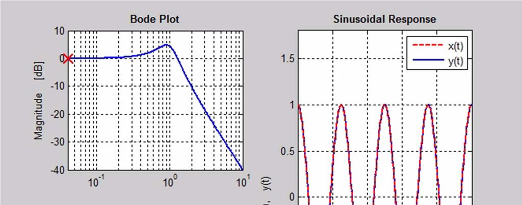
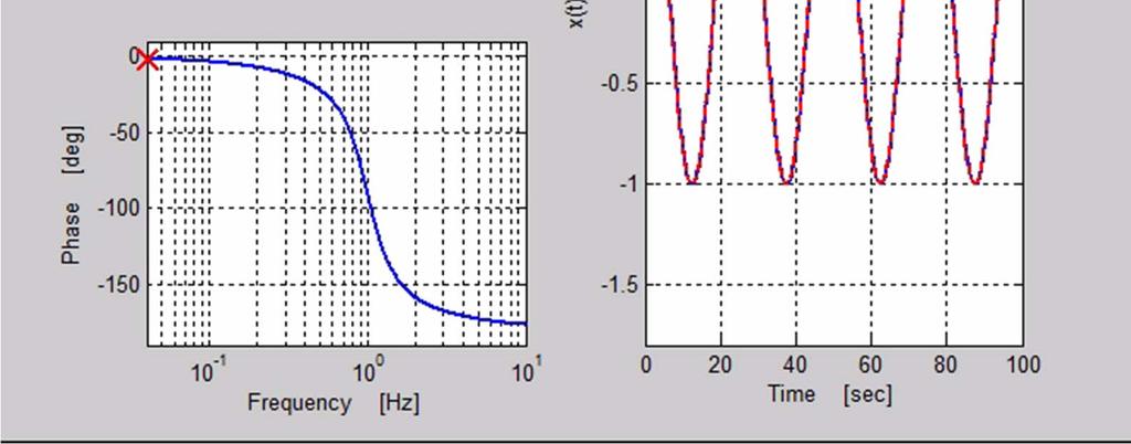
68 Time/Frequency Domain Correlation

69 69 Frequency Domain Analysis in MATLAB As was the case for time domain simulation, MATLAB has some useful functions for simulating system behavior in the frequency domain as well.

70 System Objects 70 MATLAB has data types dedicated to linear system models Two primary system model objects: State space model Transfer function model Objects created by calling MATLAB functions ss.m creates a state space model tf.m creates a transfer function model

71 State Space Model ss( ) 71 A: system matrix B: input matrix C: output matrix D: feed through matrix sys = ss(a,b,c,d) sys: state space model object State space model object will be used as an input to other MATLAB functions

72 Transfer Function Model tf( ) 72 sys = tf(num,den) Num: vector of numerator polynomial coefficients Den: vector of denominator polynomial coefficients sys: transfer function model object Transfer function is assumed to be of the form Inputs to tf( ) are Num = [b1,b2,,br+1]; Den = [a1,a2,,an+1];

73 Frequency Response Simulation bode( ) 73 [mag,phase] = bode(sys,w) sys: system model state space, transfer function, or other w: optional frequency vector in rad/sec mag: system gain response vector phase: system phase response vector in degrees If no outputs are specified, bode response is automatically plotted preferable to plot yourself Frequency vector input is optional If not specified, MATLAB will generate automatically May need to do: squeeze(mag) and squeeze(phase) to eliminate singleton dimensions of output matrices

74 Log spaced Vectors logspace( ) 74 f= logspace(x0,x1,n) x0: first point in f is 10 x1: last point in f is 10 N: number of points in f f: vector of logarithmically spaced points Generates and logarithmically spaced points between Useful for generating independent variable vectors for log plots (e.g., frequency vectors for bode plots) Linearly spaced on a logarithmic axis