Hashemite University Mechatronics Engineering Department Mechatronics Systems Laboratory Manual

Transcription

1 Hashemite University Mechatronics Engineering Department Mechatronics Systems Laboratory Manual Prepared By: Eng.Shatha AlQadomi Eng.Sarah AlBarguothi

2 The Hashemite University Faculty of Engineering Department of Mechatronics Engineering Mechatronics Systems Lab. Experiment 1 Objectives: - Introduce the student to LabVIEW software. - Design simple LabVIEW programs to demonstrate the importance of LabVIEW software in engineering application. Apparatus: LabVIEW software downloaded on the laboratory PCs. Theoretical Background: Part 1: Getting Started with LabVIEW Virtual Instruments LabVIEW programs are called virtual instruments, or VIs, because their appearance and operation imitate physical instruments, such as oscilloscopes and multimeters. LabVIEW contains a comprehensive set of tools for acquiring, analyzing, displaying, and storing data, as well as tools to help you troubleshoot code you write. In LabVIEW, you build a user interface, or front panel, with controls and indicators. Controls are knobs, push buttons, dials, and other input mechanisms. Indicators are graphs, LEDs, and other output displays. After you build the front panel, you add code using VIs and structures to control the front panel objects. The block diagram contains this code. You can use LabVIEW to communicate with hardware such as data acquisition, vision, and motion control devices, as well as GPIB, PXI, VXI, RS232, and RS485 instruments. Part 2: Launching the LabVIEW Environment When you launch LabVIEW, the Getting Started window appears as shown by Figure 1.1. Use the Getting Started window to create new projects and VIs. You can create items from scratch or from templates and samples. You can also open existing LabVIEW files and access LabVIEW community resources and help. The Getting Started window disappears when you open an existing file or create a new file, and reappears when you close all open front panels and block diagrams. You can display the window at any time by selecting View»Getting Started Window. Exp 1: Introduction to LabVIEW 1 of 22

3 Projects Figure 1.1: LabVIEW Getting Started Window VIs are LabVIEW programs, and you can use multiple VIs together to make a LabVIEW application. To group these application-related VIs together, use a LabVIEW project. When you save a LabVIEW project from the Project Explorer window, LabVIEW creates a project file (.lvproj), that includes references to all the LabVIEW files and non-labview files in the project, configuration information, build information, and deployment information. The Project Explorer window includes the following items by default: Project root Contains all other items in the Project Explorer window. The label on the project root includes the filename for the project. My Computer Represents the local computer as a target in the project. Dependencies Includes VIs and items that VIs under a target require. Build Specifications Includes build configurations for source distributions and other types of builds available in LabVIEW toolkits and modules. If you have the LabVIEW Professional Development System or Application Builder installed, you can use Build Specifications to configure stand-alone applications, shared libraries, installers, and zip files. Part 3: VI Components A VI contains the following three components: 1- Front panel Serves as the user interface. Exp 1: Introduction to LabVIEW 2 of 22

4 2- Block diagram Contains the graphical source code that defines the functionality of the VI. 3- Icon and connector pane Identifies the interface to the VI so that you can use the VI in another VI. A VI within another VI is called a subvi. A subvi corresponds to a subroutine in text-based programming languages. 1. Front Panel The front panel, shown as follows, is the user interface of the VI. You build the front panel using controls and indicators, which are the interactive input and output terminals of the VI, respectively. Controls are knobs, push buttons, dials, and other input mechanisms. Indicators are graphs, LEDs, and other output displays. Controls simulate instrument input mechanisms and supply data to the block diagram of the VI. Indicators simulate instrument output mechanisms and display data the block diagram acquires or generates. Figure 1.2: Front Panel Window Figure 1.3: Front Panel Toolbar 2 Click the Run button to run a VI. LabVIEW compiles the VI, if necessary. You can run a VI if the Run button appears as a solid white arrow, in 1. The solid white arrow also indicates you can use the VI as a subvi if you create a connector pane for the VI. While the VI runs, the Run button appears as shown in 2 if the VI is a top-level VI, meaning it has no callers and therefore is not a subvi. If the VI that is running is a subvi, the Run button appears as shown in 3. The Run button appears broken when the VI you are creating or editing contains errors. If the Run button still appears broken as in 4 after you finish wiring the block diagram, the VI is broken and cannot run. Click this button to display the Error list window, which lists all errors and warnings Exp 1: Introduction to LabVIEW 3 of 22

5 Click the Run Continuously button to run the VI until you abort or pause execution. You also can click the button again to disable continuous running. While the VI runs, the Abort Execution button appears. Click this button to stop the VI immediately if there is no other way to stop the VI. If more than one running top-level VI uses the VI, the button is dimmed. Click the Pause button to pause a running VI. When you click the Pause button, LabVIEW highlights on the block diagram the location where you paused execution, and the Pause button appears red. Click the Pause button again to continue running the VI. The following buttons are used to control the size and position of objects on the front panel. 2. Block Diagram After you build the front panel, you add code using graphical representations of functions to control the front panel objects. The block diagram contains this graphical source code, also known as G code or block diagram code. Front panel objects appear as terminals on the block diagram. Figure 1.4: Block Diagram Window Exp 1: Introduction to LabVIEW 4 of 22

6 VI contains several primary block diagram objects terminals, functions, and wires. a. Terminals The terminals represent the data type of the control or indicator. You can configure front panel controls or indicators to appear as icon or data type terminals on the block diagram. By default, front panel objects appear as icon terminals. For example, a knob icon terminal, shown as follows, represents a knob on the front panel. The DBL at the bottom of the terminal represents a data type of double-precision, floating-point numeric. A DBL terminal, shown as follows, represents a double-precision, floating-point numeric control. Terminals are entry and exit ports that exchange information between the front panel and block diagram. Data you enter into the front panel controls (a and b in the previous front panel) enter the block diagram through the control terminals. The data then enter the Add and Subtract functions. When the Add and Subtract functions complete their calculations, they produce new data values. The data values flow to the indicator terminals, where they update the front panel indicators (a+b and a-b in the previous front panel). b. Nodes Nodes are objects on the block diagram that have inputs and/or outputs and perform operations when a VI runs. They are analogous to statements, operators, functions, and subroutines in textbased programming languages. The Add and Subtract functions in the previous block diagram are examples of nodes. c. Structures Structures, a type of node, are graphical representations of the loops and case statements of textbased programming languages. Use structures on the block diagram to repeat blocks of code and to execute code conditionally or in a specific order. d. Wires You transfer data among block diagram objects through wires. In the previous block diagram, wires connect the control and indicator terminals to the Add and Subtract functions. Each wire has a single data source, but you can wire it to many VIs and functions that read the data. Wires are different colors, styles, and thicknesses, depending on their data types. A broken wire Exp 1: Introduction to LabVIEW 5 of 22

7 appears as a dashed black line with a red X in the middle. Broken wires occur for a variety of reasons, such as when you try to wire two objects with incompatible data types. Table 1.1: Data Types in LabVIEW Block Diagram Toolbar Figure 1.5 shows the elements of the block diagram toolbar. Figure 1.5: Block Diagram Toolbar 1) Click the Highlight Execution button to display an animation of the block diagram execution when you run the VI. Notice the flow of data through the block diagram. Click the button again to disable execution highlighting. 2) Click the Retain Wire Values button to save the wire values at each point in the flow of execution so that when you place a probe on the wire you can immediately retain the most recent value of the data that passed through the wire. You must successfully run the VI at least once before you can retain the wire values. 3) Click the Step Into button to open a node and pause. When you click the Step Into button again, it executes the first action and pauses at the next action of the subvi or structure. You also can press the <Ctrl> and down arrow keys. Single-stepping through a VI steps through the VI node by node. Each node blinks to denote when it is ready to execute. 4) Click the Step Over button to execute a node and pause at the next node. You also can press the <Ctrl> and right arrow keys. By stepping over the node, you execute the node without singlestepping through the node. 5) Click the Step Out button to finish executing the current node and pause. When the VI finishes executing, the Step Out button is dimmed. You also can press the <Ctrl> and up arrow keys. By stepping out of a node, you complete single-stepping through the node and navigate to the next node. Exp 1: Introduction to LabVIEW 6 of 22

8 6) Click the Clean Up Diagram button to automatically reroute all existing wires and rearrange objects on the block diagram to generate a cleaner layout. To configure the clean up options, select Tools»Options to display the Options dialog box and select Block Diagram from the Category list. You can configure the settings in the Block Diagram Cleanup section. 3. Icon and Connector Pane After you build a VI front panel and block diagram, build the icon and the connector pane so you can use the VI as a subvi. The icon and connector pane correspond to the function prototype in text-based programming languages. Every VI displays an icon, such as the one shown as follows, in the upper right corner of the front panel and block diagram windows. A VI icon is a graphical representation of a VI. It can contain text, images, or a combination of both. If you use a VI as a subvi, the icon identifies the subvi on the block diagram of the VI. If you add the VI to a palette, the VI icon also appears on the Functions palette. You can doubleclick the icon in the front panel window or block diagram window to customize or edit it. Note Customizing VI icons is recommended, but optional. Using the default LabVIEW icon does not affect functionality. You also need to build a connector pane, shown as follows, to use the VI as a subvi. The connector pane is a set of terminals that correspond to the controls and indicators of that VI, similar to the parameter list of a function call in text-based programming languages. The connector pane defines the inputs and outputs you can wire to the VI so you can use it as a subvi. A connector pane receives data at its input terminals and passes the data to the block diagram code through the front panel controls and receives the results at its output terminals from the front panel indicators. Part 4: Data types - Booleans have only two possible values: True or False and are indicated by green data wires. - Numerics have many sizes and representations: Integers can be signed or unsigned whole numbers and are indicated by blue data wires. Doubles and Singles are signed numbers with a decimal component and are indicated by orange data wires. Exp 1: Introduction to LabVIEW 7 of 22

9 A numeric's size is indicated in bits and determines the range of possible values. - Strings are sequences of characters and are indicated by pink data wires. - Arrays are a groups of one data type and are indicated by thicker data wires. A 1 dimensional array can be thought of as a column, a 2 dimensional array as a table, and so on. - Clusters are a groups of various data types and indicated by a thick brown data wire. - An Error Cluster is a special type of cluster used to indicate warnings and errors. Error clusters are composed of a boolean status, a numeric error code, and a string source. Note: you may need conversions between different data types: on the block diagram, right click programming>>numeric>>conversion, right click programming>>boolean. Part 5: Setting up the Connector Pane Define connections by assigning a front panel control or indicator to each of the connector pane terminals. The connector pane is located to the left of the VI icon in the upper right corner of the front panel window. When you open LabVIEW, you see a default connector pattern. Select a different terminal pattern for a VI by right-clicking the connector pane and selecting Patterns from the shortcut menu. To assign a terminal to a front panel control or indicator, click a terminal of the connector pane, then click the front panel control or indicator you want to assign to that terminal. Click an open space on the front panel window. The terminal changes to the data type color of the control to indicate that you connected the terminal. Part 6: Creating Sub VIs 1- Creating SubVIs from existing VI. Figure 1.6: Connector Pane Prepare the connector pane of the VI you intend to use as a subvi. Then from function palette, choose "Select a VI". Exp 1: Introduction to LabVIEW 8 of 22

10 2- Creating SubVIs from Sections of a VI Convert a section of a VI into a subvi by using the Positioning tool to select the section of the block diagram you want to reuse and selecting Edit»Create SubVI. An icon for the new subvi replaces the selected section of the block diagram. LabVIEW creates controls and indicators for the new subvi, automatically configures the connector pane based on the number of control and indicator terminals you selected, and wires the subvi to the existing wires. Part 7: Using SubVIs To place a subvi on the block diagram, click the Select a VI button on the Functions palette. Navigate to the VI you want to use as a subvi and double-click to place it on the block diagram. Figure 1.7: Adding a SubVI to The Block Diagram You also can place an open VI on the block diagram of another open VI. Use the Positioning tool to click the icon in the upper right corner of the front panel or block diagram of the VI you want to use as a subvi and drag the icon to the block diagram of the other VI. Part 8: Structures 1. While Loop A While Loop executes a subdiagram until a condition occurs. The While Loop is located on the Structures palette. Select the While Loop from the palette then use the cursor to drag a selection rectangle around the section of the block diagram you want to repeat. When you release the mouse button, a While Loop boundary encloses the section you selected. Add block diagram objects to the While Loop by dragging and dropping them inside the While Loop. Tip The While Loop always executes at least once. Changing the value of the controls outside the loop, does not affect the loop because the value is only read once. Exp 1: Introduction to LabVIEW 9 of 22

11 Figure 1.8: How Do While Loop Work? The iteration terminal is an output terminal that contains the number of completed iterations. The iteration terminal provides the current loop iteration count, which is zero for the first iteration. Tunnels feed data into and out of structures like While Loops. The block is the color of the data type wired to the tunnel. Data pass out of a loop after the loop terminates. Figure 1.9: While Loop Elements Use shift registers when you want to pass values from previous iterations through the loop to the next iteration. A shift register appears as a pair of terminals directly opposite each other on the vertical sides of the loop border. Initializing a shift register resets the value the shift register passes to the first iteration of the loop when the VI runs. If you do not initialize the shift register, the loop uses the value written to the shift register when the loop last executed or, if the loop has never executed, the default value for the data type. Stacked shift registers let you access data from previous loop iterations. Stacked shift register remember values from multiple previous iterations and carry those values to the next iterations. To create a stacked shift register, right-click the left terminal and select Add Element from the shortcut menu. Exp 1: Introduction to LabVIEW 10 of 22

12 If you add another element to the left terminal in the previous block diagram, values from the last two iterations carry over to the next iteration, with the most recent iteration value stored in the top shift register. The bottom terminal stores the data passed to it from the previous iteration. 2. For Loop A For Loop executes a sub diagram a set number of times. The count terminal is an input terminal whose value indicates how many times to repeat the sub diagram. The iteration count for the For Loop always starts at zero. An extra conditional terminal can be added by right clicking on the loop border. A For Loop with a conditional terminal executes until the condition occurs or until all iterations are complete, whichever happens first. The for loop may not execute at all. Figure 1.10: How Do For Loop Work? The output tunnel of the for loop can be configured by right-click the tunnel, and select Tunnel Mode» 1. Concatenating: To automatically concatenate an array leaving a loop, wire the array directly to the loop output tunnel. Selecting Concatenating appends all inputs in order, forming an output array of the same dimension as the array input wired. 2. Last Value: this mode displays the last value from the last loop iteration. 3. Indexing builds an array of higher dimension. Note: You can change when LabVIEW writes values to the loop output tunnel based on a condition. Table 1.2: For Loop Vs. While Loop For Loop Executes a set number of times unless a conditional terminal is added Can execute zero times Tunnels automatically output an array of data While Loop Stops executing only if the value at the conditional terminal meets the condition Must execute at least once Tunnels automatically output the last value Exp 1: Introduction to LabVIEW 11 of 22

13 3. Case structure A Case structure has two or more subdiagrams, or cases. Only one subdiagram is visible at a time, and the structure executes only one case at a time. An input value determines which subdiagram executes. The Case structure is similar to switch statements or if...then...else statements in text-based programming languages. The case selector label at the top of the Case structure contains the name of the selector value that corresponds to the case in the center and decrement and increment arrows on each side. Click the decrement and increment arrows to scroll through the available cases. You also can click the down arrow next to the case name and select a case from the pull-down menu. Wire an input value, or selector, to the selector terminal to determine which case executes. You must wire an integer, Boolean value, string, or enumerated type value to the selector terminal. You can position the selector terminal anywhere on the left border of the Case structure. If the data type of the selector terminal is Boolean, the structure has a True case and a False case. If the selector terminal is an integer, string, or enumerated type value, the structure can have any number of cases. If you do not specify a default case for the Case structure to handle out-of-range values, you must explicitly list every possible input value. For example, if the selector is an integer and you specify cases for 1, 2, and 3, you must specify a default case to execute if the input value is 4 or any other unspecified integer value. Part 9: Timing VIs When a loop finishes executing an iteration, it immediately begins executing the next iteration, unless it reaches a stop condition. Most often, you need to control the iteration frequency or timing. 1. Wait Functions Place a wait function inside a loop to allow a VI to sleep for a set amount of time. This allows your processor to address other tasks during the wait time. Wait functions use the millisecond clock of the operating system. a. The Wait (ms) function waits until the millisecond counter counts to an amount equal to the input you specify. This function guarantees that the loop execution rate is at least the amount of the input you specify. Exp 1: Introduction to LabVIEW 12 of 22

14 When LabVIEW calls a VI for example, if millisecond timer value is 112 ms and milliseconds to wait is 10 ms, the VI finishes when millisecond timer value equals 122 ms. b. The Wait Until Next ms Multiple function waits until the value of the millisecond timer becomes a multiple of the specified millisecond multiple. Use this function to synchronize activities. You can call this function in a loop to control the loop execution rate. When LabVIEW calls a VI for example, if millisecond multiple is 10 ms and millisecond timer value is 112 ms, the VI waits 8 more milliseconds until the millisecond timer value is 120 ms, a multiple of Elapsed Time Indicates the amount of time that has elapsed since the specified start time. Part 10: Plotting data 1. Waveform Graphs and Charts Display data typically acquired at a constant rate. a. Waveform Chart The waveform chart is a special type of numeric indicator that displays one or more plots of data typically acquired at a constant rate. Waveform charts can display single or multiple plots. Configure how the chart updates to display new data. Right-click the chart and select Advanced»Update Mode from the shortcut menu to set the chart update mode. The waveform chart maintains a history of data, or buffer, from previous updates. Exp 1: Introduction to LabVIEW 13 of 22

15 Figure 1.11: Waveform Chart b. Waveform Graphs The waveform graph displays one or more plots of evenly sampled measurements. The waveform graph plots only single-valued functions, as in y = f(x), with points evenly distributed along the x-axis, such as acquired time-varying waveforms. The following front panel shows an example of a waveform graph. Figure 1.12: Waveform Graph Note: If you want to pass multiple points per plot in a single update, wire an array of clusters of numeric values to the chart/graph. Each numeric represents a single y value point for each of the plots. You can use "Bundle" or "Merge" depending on the signal data type. Exp 1: Introduction to LabVIEW 14 of 22

16 2. XY Graphs Display data acquired at a non-constant rate and data for multivalued functions. You input the x and y data to the plot. The XY graph is a general-purpose, Cartesian graphing object that plots multivalued functions, such as circular shapes or waveforms with a varying time base. The XY graph displays any set of points, evenly sampled or not. You also can display Nyquist planes, Nichols planes, S planes, and Z planes on the XY graph. Part 12: Configuring DAQ Using LabVIEW 1. Inserting a DAQ assistant Figure 1.13: XY Graph Figure 1.14: Inserting a DAQ Assistant Exp 1: Introduction to LabVIEW 15 of 22

17 The following dialog box will open: Figure 1.15: DAQ Assistant Dialog Box - Select Acquire Signals to read inputs such as sensors and push buttons. - Select Generate Signals to write output signals such as operating leds or drive circuits. 2. Acquiring signal Selecting "Acquire signal" will open the following options: - Analog inputs: You can select the proper analog input based on the measurement you are making provided that your Data Acquisition Card supports that type of measurement. Exp 1: Introduction to LabVIEW 16 of 22

18 Figure 1.16: Analog Signals - Counter input: You can select the proper counter input based on the measurement you are making provided that your Data Acquisition Card supports that type of measurement. Counter input maybe used with encoders. Figure 1.17: Counter signals Exp 1: Introduction to LabVIEW 17 of 22

19 - Digital inputs You can select the proper digital input based on the measurement you are making provided that your Data Acquisition Card supports that type of measurement. Digital inputs have only two types: either configure the DAQ as a port where all 8 pins are dealt with as one single input or you can deal lines where each pin is used as a digital input. Figure 1.18: Digital Signals The following inputs are obtained when configuring an analog voltage input: Figure 1.19: Analog Input Voltage Channals Select the channel your hardware connected to from ai0 to ai7 and click Finish. 1. The following dialog box will open where you have to fill the following: - Max: maximum value of the input voltage you are reading as long as it doesn t exceed the maximum input voltage that can be read by the DAQ. - Min: minimum value of the input voltage you are reading as long as it doesn t exceed the minimum input voltage that can be read by the DAQ. - Terminal configuration: select "Differential" for differential inputs and "RSE" for single ended inputs. Exp 1: Introduction to LabVIEW 18 of 22

20 Figure 1.20: Configuring Analog Input Voltage - Acquisition mode: it can be "one sample" where the DAQ reads only one sample and the update rate depends on the timing of the program. You can select "N samples" where a predefined number of samples "N" is read, then the program is updated with all of the readings at once. To read another "N" samples, you have to put your DAQ inside a loop. "Continuous samples" is equivalent to "N sample" inside a loop. - Samples to read (N): what is the total number of samples you want your program to get updated with after each reading is finished. - Rate (Hz): how frequent you want your samples to get read. Its unit is S/s (sample per second). i.e. during 1sec how many samples you want read. Exp 1: Introduction to LabVIEW 19 of 22

21 How to calculate the time needed to get an update in the program (total time needed to read all the samples)? This time is calculated as follows: Time=N/Hz If you want to read 1000 sample and your rate is 1KHz then you will get an update each 1sec with 1000 sample read. If you want to read 100 sample and your rate is 1KHz then you will get an update each 0.1 sec with 100 sample read. Notes: - The Express Task at the top of the dialog box is used to test the acquired or the generated signal before finishing the configuration. - Dealing with digital inputs is not much different but will less options. 3. Generating signal Generating signals is not much different except that it has less options since mostly the actuators has much less operating signals that the variety of input signals that can be generated by measurements. Figure 1.21: Generating Output Signals It is recommended to have 6 DAQ at max. one for all the analog inputs, one for all the analog outputs, one for all the digital inputs, one for all the digital outputs, one for all the counter inputs and one for all the counter outputs. 4. Dynamic Data Type When acquiring signals from or generating signals to the actual world, these signals are called dynamic data type. Ordinary indicators and controls cant deal with such data type. You will need the following convertors: Exp 1: Introduction to LabVIEW 20 of 22

22 Figure 1.22: Dynamic Data Type Converters To obtain them, right click the block diagram the select Express from the drop down menu >> signal manipulation. The following dialog box will open when you insert DDT: Figure 1.23: Configuring "From DDT" Floating is selected when dealing with analog data while Boolean is selected for digital data. The Resulting data type is selected to meet your demand mostly for the lab application it is a Single scalar. Exp 1: Introduction to LabVIEW 21 of 22

23 Procedure: 1. Design the LabVIEW program to meet the requirements of the exercise provided by your lab supervisor. 2. Run and test your program. 3. Save it with the proper name on the proper directory. Discussion and Analysis: 1. Based on the front panel and block diagram below, if all default values are zeroes, answer the related questions: Figure 1.24: Front Panel and Block Diagram for Question 1 1. How many controls are there in the Figure? 2. How many indicators are there in the Figure? 3. What will happen if "Stop" push button is pressed after three iterations? 4. Locate the subvi in the Figure? References: LabVIEW TM Core 1 Course Manual Exp 1: Introduction to LabVIEW 22 of 22

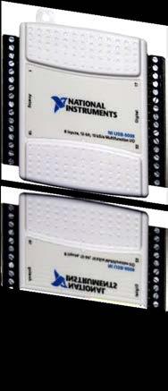
24 The Hashemite University Faculty of Engineering Department of Mechatronics Engineering Mechatronics Systems Lab. Experiment 2 Objectives: - Familiarize the student with the concept of Data Acquisition Systems. - Familiarize the student with connecting analog input/outputs, digital inputs/outputs and counter inputs/outputs to the DAC. - Learning the basic signal conditioning, interfacing and drive circuits required with DAQ. Apparatus: The systems used during this experiment are Data Acquisition Cards (DAQ) including USB 6008 DAQ. Theoretical Background: What is DAQ? Figure 2.1: USB 6008 DAQ Data acquisition (DAQ) is the process of measuring an electrical or physical phenomenon such as voltage, current, temperature, pressure, or sound with a computer. A DAQ system consists of sensors, DAQ measurement hardware, and a computer with programmable software. Compared to traditional measurement systems, PC-based DAQ systems exploit the processing power, productivity, display, and connectivity capabilities of industry-standard computers providing a more powerful, flexible, and cost-effective measurement solution. Data acquisition applications are usually controlled by software programs developed using various general purpose programming languages such as Assembly, BASIC, Fortran, LabVIEW, Java, etc. Stand-alone data acquisition systems are often called data loggers. Exp 2: Data Acquisition 1 of 11

25 A complete data acquisition system consists of: Sensors and Actuators (Plant). Signal Conditioning circuit (which in modern systems is integrated within the DAQ hardware). DAQ Measurement Hardware (Interface Devices). DAQ Software and Device Driver. Figure 2.2: Data Acquisition System Different types of DAQ cards available in the mechatronics system design laboratory include: PCI DAQ, USB DAQ, Compact DAC and Compact RIO. Part 1: Connecting Analog Current Inputs NI DAQ devices measure current by means of an internal, precision shunt resistor. Most devices can measure ± 20 ma, which maps to the output range of most current transducers and 4 ma to 20 ma current loops. Before making signal connections, check the specifications of your device. When making signal connections, you must be careful with the voltage level of the signal going into the device. You can make two types of connections: - Differential Measurements (Current Loop Measurements) Devices capable of different current measurements have two terminals per measurement channel: AI+ and AI-. Connect the positive side of the current source to the AI+ terminal, and connect the negative side of the current source to the AI terminal. Exp 2: Data Acquisition 2 of 11

26 Figure 2.3: Connecting a Differential Current Measurement This measurement is made using a DAQ containing a shunt resistor. The main components of a current loop include a DC power supply, transducer, a data acquisition device, and wires connecting them together in a series, as shown below. Figure 2.4: Current Loop System - Single-Ended Measurements (3-wire current transducer) Devices capable of single-ended measurements have one terminal per measurement channel (AI), a supply terminal and a common ground terminal (COM). Connect the positive lead of the current signal to the AI terminal. Connect the negative lead to the COM terminal. Figure 2.5: Connecting a Single-Ended Current Measurement Exp 2: Data Acquisition 3 of 11

27 Part 2: Connecting Analog Voltage Inputs - Floating Vs. Referenced Signal Sources Floating Signal Sources Figure 2.6: 3-Wire Current Transducer A floating signal source is not connected to the building ground system but has an isolated ground reference point. Some examples of floating signal sources are outputs of transformers, thermocouples, battery-powered devices, optical isolators, and isolation amplifiers. An instrument or device that has an isolated output is a floating signal source. The ground reference of a floating signal must be connected to the ground of the device to establish a local or onboard reference for the signal. Ground Referenced Signal Sources A ground referenced signal source is connected to the building system ground, so it is already connected to a common ground point with respect to the device, assuming that the measurement device is plugged into the same power system as the source. Non-isolated outputs of instruments and devices that plug into the building power system fall into this category. - Single Ended Vs. Differential Single ended Sources The voltage is measured between a point and the ground. This type of configuration allows for the DAQ system to support more channels but is susceptible to noise from the common ground. Examples for this type include outputs of NPN sensors (such as proximity), outputs of amplifier circuits and outputs of voltage divider circuits. Differential Sources The voltage is measured between two individual points within a common mode range. The measurement is independent of the ground which makes it more immune to noise. The reason for this is that the noise source is present on both signal leads and when in differential mode only the difference between the two leads is measured. Examples for this type include outputs of bridge circuits, thermocouple and strain gauges. Exp 2: Data Acquisition 4 of 11

28 The figure below shows the different types of signal source types as well as the optimal connection diagrams based on the individual measurement method. Please note that depending on the type of signal, a particular voltage measurement method may provide better results than others. Figure 2.7: Optimal Connection Diagrams for Different Types of Sources Part 3: Connecting Digital Inputs/Outputs The configurations shown below represent what the DAQ internal digital lines look like and how to deal with them. The push pull configuration (to the left) has both NPN and PNP transistors which means that it can be either a sinking or sourcing [input/output]. Either pull up or pull down resistors can be connected to it. The open collector configuration (to the right) can be used only as a sourcing [input/output]. This mode can be used only with pull up resistors. Exp 2: Data Acquisition 5 of 11

29 Figure 2.8: Push Pull Vs. Open Collector Configurations The table below illustrates the different connection of digital inputs and output to DAQ based on the system current requirements. Table 2.1: Open Collector Different connections as Input and Output Open collector as input Open collector as output Sourcing input with internal pull up Digital output without a resistor (load doesn't consume high currents) Sourcing input with external pull up, this configuration will increase the current of the input. Digital output without a resistor to decrease load current Exp 2: Data Acquisition 6 of 11

30 Digital output with external pull up resistor to increase the load current Examples for digital inputs include digital proximity sensors, push buttons and limit switches. LEDs, Buzzers and digital control signal are considered as digital outputs. Part 4: Connecting Counter Inputs/Outputs Counter inputs/outs are basically dealt with as any digital input. Part 5: Connecting Analog Output Voltage Signals Connecting analog outs is mostly a simple process. You connect the output pin to the output device and the other terminal of the device to the analog GND. Exp 2: Data Acquisition 7 of 11

31 Figure 2.9: Connecting analog outputs Sometimes the level of the voltage that operates the output device doesn t match the range of the DAQ signal. In these cases some interfacing and drive circuits maybe required such as H- bridges, inverters, optical isolators. Figure 2.10: Connecting to analog outputs using transistors 2.11: Connecting to dc motor using H-Bridge Exp 2: Data Acquisition 8 of 11

32 Part 6: Signal Conditioning 2.12: Connecting to induction motor using Inverter Many applications involve environmental or structural measurements, such as temperature and vibration, from sensors. These sensors, in turn, require signal conditioning before a data acquisition device can effectively and accurately measure the signal. Signal conditioning is one of the most important components of a data acquisition system because without optimizing realworld signals for the digitizer in use, you cannot rely on the accuracy of the measurement. The following list offers common signal conditioning types. Amplification Amplifiers increase voltage level to better match the DAQ analog-to-digital converter (ADC) range thus increasing the measurement resolution and sensitivity. Typical sensors that require amplification are thermocouples and strain gages. Attenuation Attenuation, the opposite of amplification, is necessary when voltages to be digitized are beyond the ADC range. This form of signal conditioning decreases the input signal amplitude so that the conditioned signal is within the ADC range. Attenuation is typically necessary when measuring voltages that are more than 10 V. Filtering Filters reject unwanted noise within a certain frequency range. Often, lowpass filters are used to block out noise in electrical measurements, such as 50/60 Hz power. Isolation Voltage signals well outside the range of the digitizer can damage the measurement system and harm the operator. For that reason, isolation is usually required in conjunction with attenuation to protect the system and the user from dangerous voltages or voltage spikes. Isolation may also be needed when the sensor is on a different ground plane from the measurement sensor, such as a thermocouple mounted on an engine. Exp 2: Data Acquisition 9 of 11

33 Excitation Excitation is required for many types of transducers. For example, strain gages, accelerometers thermistors, and RTDs require external voltage or current excitation. RTD and thermistor measurements are made with a current source that converts the variation in resistance to a measureable voltage. Accelerometers often have an integrated amplifier, which requires current excitation provided by the measurement device. Strain gages, which are very-low-resistance devices, are typically used in a Wheatstone bridge configuration with a voltage excitation source. Linearization Linearization is necessary when sensors produce voltage signals that are not linearly related to the physical measurement. Linearization, the process of interpreting the signal from the sensor, can be implemented either with signal conditioning or through software. A thermocouple is the classic example of a sensor that requires linearization. Procedure: 1. Inspect the USB 6008 DAQ provided by your lab supervisor. 2. Design and implement the circuit using the components available with the DAQ, to meet the requirements the task handed to you by your supervisor. 3. Using LabVIEW, design the proper program needed to operate your circuit. 4. Run your program and test your circuit. Discussion and Analysis: 1. Draw a schematic of the circuit you connected in the lab using Figure Figure 2.13: USB 6008 Pinout. Exp 2: Data Acquisition 10 of 11

34 2. Show all the calculation you made in order to select the values of the external resistors added to the circuit. References: Exp 2: Data Acquisition 11 of 11

35 The Hashemite University Faculty of Engineering Department of Mechatronics Engineering Mechatronics Systems Lab. Experiment 3 Objectives: - Familiarize the student with USB 6008 DAQ. - Study the basic features of the DAQ. Apparatus: The system used during this experiment is the USB 6008 DAQ. Theoretical Background: Figure 3.1: USB 6008 DAQ USB 6008 is the data acquisition card available in the mechatronics lab to which the students can connect their designed systems. During this experiment, the basic points related to using and connecting to USB 6008 DAQ will be illustrated by means of the data sheet of the DAQ. The National Instruments USB-6008 is a low-cost, multifunction data acquisition device (DAQ). It has 8 analog inputs, 2 analog outputs, and 12 digital input/outputs. The digital channels are divided into two ports. When one or more channels on each port is set to either input or output, the port is locked into that particular mode. Introduction The NI USB-6008/6009 provides connection to eight analog input (AI) channels, two analog output (AO) channels, 12 digital input/output (DIO) channels, and a 32-bit counter when using a full-speed USB interface. Exp 3: USB 6008 DAQ 1 of 12

36 Table 3.1: Differences between the USB-6008 and USB-6009 Feature USB-6008 USB-6009 AI Resolution 12 bits differential, 14 bits differential, Maximum AI Sample bi 10 i ks/s l dd bi 48 i ks/s l dd DIO Configuration Open-drain Open-drain or push-pull Hardware Open drain is the same as open collector The following block diagram shows key functional components of the USB-6008/6009. From DAQ: the DAQ can supply any external circuit with 5 V provided that the total current consumed by all circuits doesn t exceed 200mA. Only input counter Configurable as input or output using the program Very low current output Analog inputs; 4 differential or 8 single ended 2 analog outputs Figure 3.2: Device block diagram Exp 3: USB 6008 DAQ 2 of 12

37 Signal Description Table 3.2 describes the signals available on the I/O connectors. Table 3.2 Signal Descriptions Signal Name Reference Direction Description GND Ground The reference point for the single-ended AI measurements, bias current return point for differential mode measurements, AO voltages, digital signals at the I/O connector, +5 VDC supply, and the +2.5 VDC reference. AI <0..7> Varies Input Analog Input Channels 0 to 7 For single-ended measurements, each signal is an analog input voltage channel. For differential measurements, AI 0 and AI 4 are the positive and negative inputs of differential analog input channel 0. The following signal pairs also form differential input channels: <AI 1, AI 5>, <AI 2, AI 6>, and <AI 3, AI 7>. AO 0 GND Output Analog Channel 0 Output Supplies the voltage output of AO channel 0. AO 1 GND Output Analog Channel 1 Output Supplies the voltage output of AO channel 1. P1.<0..3> P0.<0..7> GND Input or Output Digital I/O Signals You can individually configure each signal as an input or output V GND Output +2.5 V External Reference Provides a reference for wrap-back testing. +5 V GND Output +5 V Power Source Provides +5 V power up to 200 ma. PFI 0 GND Input PFI 0 This pin is configurable as either a digital trigger or an event counter input. Exp 3: USB 6008 DAQ 3 of 12

38 Analog Input You can connect analog input signals to the USB-6008/6009 through the I/O connector. Refer to Table 3.3 for more information about connecting analog input signals. Analog Input Circuitry Figure 3.3 illustrates the analog input circuitry of the USB-6008/6009. The mux selects 1 channel to read at a time - MUX Figure 3.3: Analog Input Circuitry The USB 6008/6009 has one analog-to-digital converter (ADC). The multiplexer (MUX) routes one AI channel at a time to the PGA. - PGA The programmable-gain amplifier provides input gains of 1, 2, 4, 5, 8, 10, 16, or 20 when configured for differential measurements and gain of 1 when configured for single-ended measurements. The PGA gain is automatically calculated based on the voltage range selected in the measurement application. - A/D Converter The analog-to-digital converter (ADC) digitizes the AI signal by converting the analog voltage into a digital code. - AI FIFO The USB-6008/6009 can perform both single and multiple A/D conversions of a fixed or infinite number of samples. A first-in-first-out (FIFO) buffer holds data during AI acquisitions to ensure that no data is lost. Exp 3: USB 6008 DAQ 4 of 12

39 Analog Input Modes You can configure the AI channels on the USB-6008/6009 to take single-ended or differential measurements. - Connecting Differential Voltage Signals For differential signals, connect the positive lead of the signal to the AI+ terminal, and the negative lead to the AI terminal. Figure 3.4: Connecting a Differential Voltage Signal Peak to peak voltage The differential input mode can measure ±20 V signals in the ±20 V range. However, the maximum voltage on any one pin is ±10 V with respect to GND. For example, if AI 1 is +10 V and AI 5 is 10 V, then the measurement returned from the device is +20 V. - Connecting Reference Single-Ended Voltage Signals To connect reference single-ended voltage signals (RSE) to the USB-6008/6009, connect the positive voltage signal to the desired AI terminal, and the ground signal to a GND terminal. Figure 3.5: Connecting a single ended Voltage Signal Exp 3: USB 6008 DAQ 5 of 12

40 Analog Output The USB-6008/6009 has two independent AO channels that can generate outputs from 0 5 V. All updates of AO lines are software-timed. Analog Output Circuitry Figure 3.6 illustrates the analog output circuitry for the USB-6008/6009. DACs Figure 3.6: Analog Output Circuitry Connecting a Load Digital-to-analog converts (DACs) convert digital codes to analog voltages. - Connecting Analog Output Loads The 50Ω output resistor must be accounted of when connecting loads. To connect loads to the USB-6008/6009, connect the positive lead of the load to the AO terminal, and connect the ground of the load to a GND terminal. Digital I/O Figure 3.7: Connecting a Load The USB-6008/6009 has 12 digital lines, P0.<0..7> and P1.<0..3>, which comprise the DIO port. GND is the ground-reference signal for the DIO port. You can individually program all lines as inputs or outputs. Digital I/O Circuitry Figure 3.8 shows P0.<0..7> connected to example signals configured as digital inputs and digital outputs. You can configure P1.<0..3> similarly. Exp 3: USB 6008 DAQ 6 of 12

41 This configuration is not valid in DAQ 6008 Source/Sink Information Figure 3.7: Example of Connecting a Load The default configuration of the USB-6008/6009 DIO ports is open-drain, allowing 5 V operations, with an onboard 4.7 kω pull-up resistor. An external, user-provided, pull-up resistor can be added to increase the source current drive up to a 8.5 ma limit per line as shown in Figure 3.8. This resistor is an internal pull resistor inside the DAQ, so it is NOT a necessity to add an external pull up resistor when connection a digital input. In this case you are limited to a current of 0.6mA.You may add an external resistor in case you want to increase the output current to its full capacity of 8.5mA. Figure 3.8: Example of Connecting External User-Provided Resistor Exp 3: USB 6008 DAQ 7 of 12

42 Complete the following steps to determine the value of the user-provided pull-up resistor: 1. Place an ammeter in series with the load. 2. Place a variable resistor between the digital output line and the +5 V. 3. Adjust the variable resistor until the ammeter current reads as the intended current. The intended current must be less than 8.5 ma. 4. Remove the ammeter and variable resistor from your circuit. 5. Measure the resistance of the variable resistor. The measured resistance is the ideal value of the pull-up resistor. 6. Select a static resistor value for your pull-up resistor that is greater than or equal to the ideal resistance. 7. Re-connect the load circuit and the pull-up resistor. Power-On States At system startup and reset, the hardware sets all DIO lines to high-impedance inputs. The DAQ device does not drive the signal high or low. Each line has a weak pull-up resistor connected to it. At floating conditions(when the program is not running and the input or output state is decided), during such cases the pull resistor will case 5V to appear at the digital pin regardless it is configured as input or output. Event Counter You can configure PFI 0 as a source for a gated invertor counter input edge count task. In this mode, falling-edge events are counted using a 32-bit counter. Only works at falling edges and is used as input Specifications The following specifications are typical at 25 C, unless otherwise noted. Analog Input Number of bits reflected the size of the register in the microprocessor used in the ADC process Resolution=Vin(max)/ (2^(number of bits) -1) Resolution is defined as the minimum voltage change required to be detected by DAQ Converter type... Successive approximation Analog inputs... 8 single-ended/4 differential, software selectable Input resolution USB bits differential, 11 bits single-ended Exp 3: USB 6008 DAQ 8 of 12

43 USB bits differential, 13 bits single-ended Max sampling rate USB ks/s USB ks/s Up to how many samples can the DAQ acquire during a second S/s: Sample per second Input range Single-ended... ±10 V Differential... ±20 V, ±10 V, ±5 V, ±4 V, Peak to peak voltage ±2.5 V, ±2 V, ±1.25 V, ±1 V Working voltage... ±10 V Input impedance kω Overvoltage protection... ±35 Input impedance: high input impedance which means that the DAQ will not draw current from analog input devices reducing the loading effect (ideally this value should be infinity Analog Output Converter type...successive approximation Analog outputs 2 Output resolution...12 bits Resolution= Vout(max)/((2^12)-1) Maximum update rate Hz, software-timed Power-on state...0 V Output range...0 to +5 V Exp 3: USB 6008 DAQ 9 of 12

44 Output impedance...50 Ω Output current drive...5 ma Each analog output has an on-board 50Ω resistor and can drive loads with a maximum current of 5mA. Figure 3.9: Analog output calculations Digital I/O P0.<0..7>... 8 lines PI.<0..3>... 4 lines Direction control... Each channel individually programmable as input or output Output driver type USB Open-drain Open collector USB Each channel individually programmable as push-pull or open-drain Compatibility... TTL, LVTTL, CMOS Absolute maximum voltage range to 5.8 V with respect to GND Pull-up resistor kω to 5 V Power-on state... Input (high impedance) Exp 3: USB 6008 DAQ 10 of 12

45 Table 3.3 Signal Descriptions Level Min Max Units Input low voltage V Input high voltage When used as input V Input leakage current 50 µa Output low voltage (I = 8.5 ma) 0.8 V Output high voltage Not supported by DAQ 6008 Push-pull, I = 8.5mA V Open-drain, I = 0.6mA, nominal V Open-drain, I = 8.5mA, with external pull-up resistor 2.0 V When used as output Only 4.7KΩ onboard the Counter Number of counters Resolution...32 bits Counter measurements...edge counting (falling-edge) Pull-up resistor kω to 5 V Maximum input frequency...5 MHz Bus Interface Power Requirements External Voltage USB specification...usb 2.0 full-speed USB bus speed...12 Mb/s USB 4.10 to 5.25 VDC...80 ma typical, 500 ma max USB suspend µa typical, 500 µa max +5 V output (200 ma maximum) V typical, V minimum +2.5 V output (1 ma maximum) V typical Very low current; the supply is used for self test only Exp 3: USB 6008 DAQ 11 of 12

46 Procedure: 1. Inspect the USB 6008 DAQ provided by your lab supervisor. 2. Design and implement the circuit using the components available with the DAQ, to meet the requirements of your design problem. 3. Using LabVIEW, design the proper program needed to operate your circuit. 4. Run your program and test your circuit. Discussion and Analysis: 1. Draw a schematic of the circuit you connected in the lab using Figure Figure 3.10: USB 6008 Pinout. 2. Show all the calculation you made in order to select the values of the external resistors added to the circuit. Exp 3: USB 6008 DAQ 12 of 12

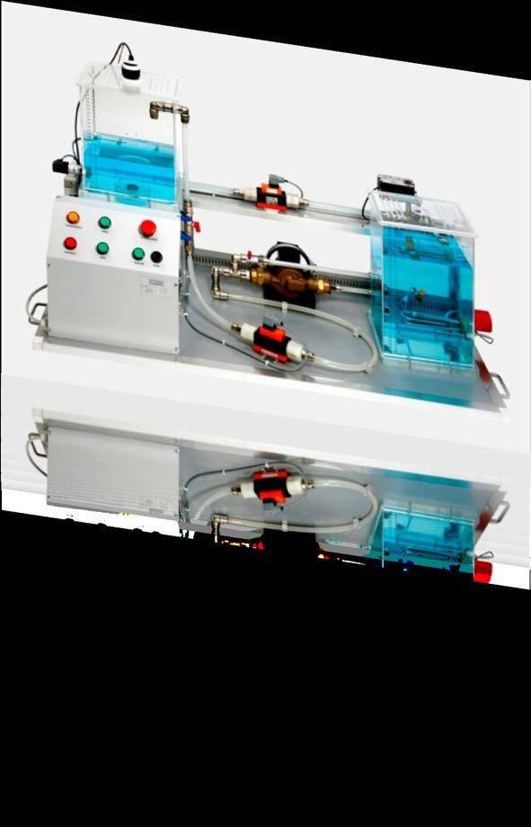
47 The Hashemite University Faculty of Engineering Department of Mechatronics Engineering Mechatronics Systems Lab. Experiment 4 Objectives: - Familiarize the student with the process trainer system (PT001). - Lean how to model simple level and flow control systems. Apparatus: The system used during this experiment is the PT001 System. Theoretical Background: Figure 4.1: PT001 Trainer The PT001 Process Trainer is a bench-mounted, Process Trainer for Level, Flow, Temperature, and Pressure control. It comprises all the required sensors to perform the many control operations. Exp 4: Process Trainer System 1 of 11

48 1. Hardware: a. Description: The setup consists of the following components: Figure 4.2: Indicated Components for the Process Trainer System Table 4.1: The Components of the Process Trainer System 1. Electric Control Box 2. Tank 1 3. Tank 2 4. Pressure Sensor 5. Ultrasonic Level Meter 6. Thermocouple Tank 1 7. Thermocouple Tank2 8. Flow Meter (Upper) 9. Flow Meter (Lower) 10. Electric Flow Control Valve 11. Manual Flow Control Valve 12. Heater 13. Pump 14. Level Switch Exp 4: Process Trainer System 2 of 11

49 The main buttons of the Electric Control Box are as follows: Figure 4.3: Indicated Components for the Process Trainer System Table 4.2: The Components of the Process Trainer System 1. Emergency Switch 2. Main Power 3. Pump Indicator 4. Level Alarm 5. Process Indicator 6. Heater Indicator b. Specifications: Table 4.3 summarizes the specification related to the sensors and actuators of the system. These specifications are important when you want to configure the DAQ assistant in the LabVIEW programs need to run the process trainer. Table 4.3: Sensors and Actuators specifications 1. Pressure Sensor Measuring Range: 0 to 0.1 bar Supply Voltage: 24 VDC Output: 4-20mA Temperature Range: 0-80 ºC Media: Water Housing: Stainless Steel Accuracy: ±0.5% of the full range 2. J-Type Thermocouple Type: J-Type With Protective Tube Immersion Length: 10 cm Exp 4: Process Trainer System 3 of 11

50 3. Ultrasonic Level Meter Measuring Range: 5 to 30 cm Supply Voltage: 24 VDC Output: 4-20mA Temperature Range: ºC Accuracy: ±0.15% of span in air Dead Band: 5 cm 5. Level Switch Temperature: -10º - 50º Pressure: 100 psig 7. Pump Power: 0.17 HP Supply Voltage: 220 VAC, Single Phase Maximum Fluid Temperature: 100 ºC 9. Inline Flow sensors Measuring Range: L/min Supply Voltage: 24 VDC Output: 4-20 ma Temperature Range: 0-60 ºC 4. Flow Control Valve Supply Voltage: 24 VAC Control Signal: 0 10 VDC Feedback Signal: 0-10 VDC Angle of Rotation: 0º - 95º Running Time: 108 sec 6. Heater Power: 1200 W Supply Voltage: 220 VAC, Single Phase 8. Variable Speed Drive Motor Output Rating: 0.5 HP Supply Voltage/ Phases: 220/ 1Ø Output Voltage/ Phases: 0-240/ 1Ø Supply Frequency: 48 to 62 Hz Max. Ambient Temperature 50 ºC Storage Temperature ºC 10. Plexiglas Tanks Maximum Medium Temperature: 70 ºC Medium: Water c. Data Acquisition: The acquisition system is done with sensors and actuators are connected to a Compact DAQ. Compact DAQ USB chassis provide the plug-and-play simplicity of USB to sensor and electrical measurements on the benchtop, in the field, and on the production line. By combining more than 50 sensor-specific NI C Series I/O modules with patented NI Signal Streaming technology, the NI Compact DAQ platform delivers high-speed data and ease of use in a flexible, mixedmeasurement system. The DAQ system in the lab is composed from a chassis and 4 modules as illustrated below. Exp 4: Process Trainer System 4 of 11

51 Figure 4.4: cdaq & Its Modules 1. National Instruments, NI CompactDAQ 4-Slot USB Chassis (NI cdaq-9174) Choose from more than 50 hot-swappable I/O modules with integrated signal conditioning Four general-purpose 32-bit counter/timers built into chassis (access through digital module) Run up to seven hardware-timed analog I/O, digital I/O, or counter/timer operations simultaneously Stream continuous waveform measurements with patented NI Signal Streaming technology 2. National Instruments 16-Channel AI (8 Voltage and 8 Current) (NI 9207) 8 current inputs (±21.5 ma) and 8 voltage (±10 V) High-resolution mode with 50/60 Hz rejection 500 S/s sample rate (high-speed mode) Vsup pins for external power routing (2 A/30 V max) 3. National Instruments 4-Channel, 100 ks/s, 16-bit, ±10 V, Analog Output Module (NI 9263) 4 simultaneously updated analog outputs, 100 ks/s 16-bit resolution Hot-swappable operation 4. National Instruments 4-Channel, 14 S/s, 24-Bit, ±80 mv Thermocouple Input Module (NI 9211) 4 thermocouple or ±80 mv analog inputs 24-bit resolution; 50/60 Hz noise rejection Exp 4: Process Trainer System 5 of 11

52 Hot-swappable operation NIST-traceable calibration 5. National Instruments 8-Channel 24 V Logic, 100 μs, Sourcing Digital Output Module (NI 9472) 8-channel, 100 μs digital output 6 to 30 V range, sourcing digital output D-Sub or screw-terminal connector options Hot-swappable operation Extreme industrial certifications/ratings The voltage ranges and DAQ module numbers are necessary when configuring the DAQ assistant. d. Hardware Connection: Table 4.4 illustrates the connection of the sensors and actuators to their proper modules and channels. 2. Software The system is driven by means of LabVIEW programs designed from the manufacturer or else designed by the students to meet certain requirements. Figure 4.5: Manufacturer Designed Software Exp 4: Process Trainer System 6 of 11

53 Table 4.4: Connection Table 3. Fluid System Modeling In fluid systems there are three basic building blocks: Resistance, capacitance and inertance. Figure 4.6: Hydraulic examples: (a) resistance, (b) capacitance, (c) inertance Exp 4: Process Trainer System 7 of 11

54 1. Fluid Resistance Hydraulic resistance is the resistance to flow which occurs as a result of a liquid flowing through valves or changes in a pipe diameter. The relationship between the change in flow rate of liquid q through the resistance element and the resulting pressure difference (p1 p2) is given as (4.1) P P R * q 1 2 = Where R is a constant called the hydraulic resistance. The higher the resistance, the higher the pressure difference for a given rate of flow. Equation 4.1 like that for the electrical resistance and Ohm s law, assumes a linear relationship. Such hydraulic linear resistances occur with orderly flow through capillary tubes and porous plugs but nonlinear resistances occur with flow through sharp-edge orifices or if the flow is turbulent. 2. Hydraulic Capacitance Figure 4.7: Hydraulic Resistance Hydraulic capacitance is the term used to describe energy storage with a liquid where it is stored in the form of potential energy as shown in Figure 4.8. A height of liquid in the container shown in Figure 4.8 (called pressure head) is one form of such storage. Figure 4.8: Hydraulic Capacitance For such a capacitance, the rate of change of volume V in the tank (dv/dt) is equal to the difference between the volumetric rate at which liquid enters the container q1 and the rate at which it leaves the container q2 q q = 2 dv dt 1 (4.2) Exp 4: Process Trainer System 8 of 11

55 But V = Ah, where A is the cross-sectional area of the container and h is the height of liquid in it. Hence d( Ah) q q2 = = dt dh A dt 1 (4.3) The pressure difference between the input and output is p, where p = hρg with ρ being the liquid density and g the acceleration due to gravity. Therefore, if the liquid is assumed to be incompressible (density does not change with pressure), then Equation (4.3) can be written as q q The hydraulic capacitance C is defined as d( p / ρg) = dt A dp = ρg dt 1 2 (4.4) Therefore C A ρ g = (4.5) dp q q 2 = C dt 1 (4.6) 3. Hydraulic Inertance Hydraulic inertance is the equivalent of inductance in electrical systems or a spring in mechanical systems. To accelerate a fluid and to increase its velocity a force is required. Consider a block of liquid of mass m as shown in Figure 4. The net force acting on the liquid is Figure 4.9: Hydraulic Inertance F F = p A p A = p p ) A ( 1 2 (4.7) Where (p1 p2) is the pressure difference and A the cross-sectional area. This net force causes the mass to accelerate with an acceleration a, and so Exp 4: Process Trainer System 9 of 11

56 ( 2 p p ) A = ma However, a is the rate of change of velocity dv/dt, therefore 1 (4.8) dv p p ) A = m dt ( 2 1 (4.9) The mass of liquid concerned has a volume of AL, where L is the length of the block or the distance between the points in the liquid where the pressures p1 and p2 are measured. If the liquid has a density ρ then m = ALρ, and ( p p2) A = But the volume rate of flow q = Av, hence p dv ALρ dt 1 (4.10) dq p ) A = Lρ dt ( 2 1 (4.11) dq p p ) = I dt ( 2 Where the hydraulic inertance I is defined as 1 (4.12) I Lρ A = (4.13) The following system represents the system laboratory: Figure 4.10: Process Trainer System Exp 4: Process Trainer System 10 of 11

57 Procedure: 1. Inspect Tables 4.3 and Design a LabVIEW program to meet the task provided by your lab supervisor. You may need the following formulas: - For the ultrasonic level meter : H= *I For any analog signal, select "one sample on demand". - The flow control valve at 0V is fully opened. 3. Fill the following Table to help you configure your DAQ assistant. Table 4.5: Hardware Configuration Actuator1 Sensor1 Actuator2 Sensor2 Input/output Digital/Analog Discussion and Analysis: Signal type (voltage/current) Range of Signal Module name Channel number 1. How many sensors are there in the system you designed? List them? 2. How many actuator are there in the system you designed? List them? 3. Draw a flow chart of the program you designed. 4. How many DAQ assistant you used in your program? What are their types? 5. How many samples per second do the analog modules support? References: 1. Mechatronics: electronic control systems in mechanical and electrical engineering, 4 th edition, W.Bolton. Exp 4: Process Trainer System 11 of 11

58 The Hashemite University Faculty of Engineering Department of Mechatronics Engineering Mechatronics Systems Lab. Experiment 5 Objectives: - Familiarize the student with the concept of PID controller. - Study the effect of each action of the PID controller. - Learn how tune the PID controller gains. Apparatus: The system used during this experiment is the PT001 System. Theoretical Background: Introduction: Figure 5.1: PT001 Trainer Proportional-Integral-Derivative (PID) control is the most common control algorithm used in the industry and has been universally accepted in industrial control. The popularity of PID controllers can be attributed partly to their robust performance in a wide range of operating Exp 5: PID Controller: Concept and Tuning 1 of 7

59 conditions and partly to their functional simplicity, which allows engineers to operate them easily. As the name suggests, PID algorithm consists of three basic coefficients; proportional, integral and derivative, which are varied to get optimal response. de( t) PID = K p * e( t) + Ki * e( t) dt + Kd * (5.1) dt - Proportional Response Figure 5.2: PID Controller Algorithm The proportional component depends only on the difference between the setpoint and the process variable. This difference is referred to as the Error term. The proportional gain (Kc) determines the ratio of output response to the error signal. For instance, if the error term has a magnitude of 10, a proportional gain of 5 would produce a proportional response of 50. In general, increasing the proportional gain will increase the speed of the control system response. However, if the proportional gain is too large, the process variable will begin to oscillate. If Kc is increased further, the oscillations will become larger and the system will become unstable and may even oscillate out of control. - Integral Response P K * e( t) out = p (5.2) The integral component summates the error term over time. The result is that even a small error term will cause the integral component to increase slowly. The integral response will continually increase over time unless the error is zero, so the effect is to drive the Steady-State error to zero. Steady-State error is the final difference between the process variable and setpoint. A phenomenon called integral windup results when integral action saturates a controller without the controller driving the error signal toward zero. I = K e( t dt out i ) * (5.3) Exp 5: PID Controller: Concept and Tuning 2 of 7

60 - Derivative Response The derivative component causes the output to decrease if the process variable is increasing rapidly. The derivative response is proportional to the rate of change of the process variable. Increasing the derivative time (Td) parameter will cause the control system to react more strongly to changes in the error term and will increase the speed of the overall control system response. Most practical control systems use very small derivative time (Td), because the Derivative Response is highly sensitive to noise in the process variable signal. If the sensor feedback signal is noisy or if the control loop rate is too slow, the derivative response can make the control system unstable. D out T d de( t) * dt = (5.4) Table 5.1: PID controller's Elemet Actions PID Tuning Using Ziegler and Nichols Ziegler and Nichols described simple mathematical procedures, the first and second methods respectively, for tuning PID controllers. These procedures are now accepted as standard in control systems practice. Both techniques make a priori assumptions on the system model, but do not require that these models be specifically known. Ziegler-Nichols formula for specifying the controllers are based on plant step responses. - The First Method The first method is applied to plants with step responses of the form displayed in Figure 5.3 (response exhibit s-shaped curve for unit step input). This type of response is typical of a first order system with transportation delay, such as that induced by fluid flow from a tank along a pipe line. It is also typical of a plant made up of a series of first order systems. The response is characterized by two parameters, L the delay time and T the time constant. These are found by drawing a tangent to the step response at its point of inflection and noting its intersections with the time axis and the steady state value. The plant model is therefore G(s) =, Ziegler and Nichols derived the following control parameters based on this model which is describes in Table 5.2: Exp 5: PID Controller: Concept and Tuning 3 of 7

61 Figure 5.3: First Order S-Shape Response Table 5.2: PID Controller Tuning Using Ziegler-Nichols First Method Notes: Using this method, the tuning is done for closed loop system. Complete PID is considered unnecessary because it is a first order system that sustains no oscillations; thus no need for the derivative action. - The Second Method The second method targets plants that can be rendered unstable under proportional control. The technique is designed to result in a closed loop system with 25% overshoot. This is rarely achieved as Ziegler and Nichols determined the adjustments based on a specific plant model. The steps for tuning a PID controller via the 2 nd method are as follows: Exp 5: PID Controller: Concept and Tuning 4 of 7

62 Using only proportional feedback control: 1. Reduce the integrator and derivative gains to Increase Kp from 0 to some critical value Kp=Kcr at which sustained oscillations occur. If it does not occur then another method has to be applied. 3. Note the value Kcr and the corresponding period of sustained oscillation, Pcr. The controller gains are now specified as follows in Table 5.3. Figure 5.4: Second Order Response Table 5.3: PID Controller Tuning Using Ziegler-Nichols Second Method Note: using this method, the tuning is done for closed loop system. Exp 5: PID Controller: Concept and Tuning 5 of 7

63 Process Trainer System For the Process Trainer System in the labratory, the PID Feedback Level Experiment, the PID level controller takes the feedback signal from the level meter and compares it with the desired value of level (Setpoint) and accordingly gives a control signal to the pump to deliver the required water flow & maintain the level at the desired value. The same principle is applied to the pressure and flow controllers, except that the feedback signal is taken from the pressure sensor and the flow meter respectively. This type of controllers rejects the disturbances after they affect the PV (Water Level) Procedure: Figure 5.5: PID Level Control Implementation in PT Click on Experiment 3: PID Feedback Control. Another menu will appear; choose Experiment 3.1: PID Feedback Level Control. 2. Drag the Setpoint slider to 30% of its value. Press the [Start Process] button to start the control process. Observe the behavior of the (PV) and the controller s output on the chart. 3. After the controller and (PV) settle down and stabilize, apply a disturbance to the system by changing the Flow Control Valve s opening. Observe the disturbance rejection and the reaction of the controller. Exp 5: PID Controller: Concept and Tuning 6 of 7

64 4. Set the Flow Control Valve to Fully Open, and change the setpoint to 60%. When the level settles at 60% of its full scale, observe the behavior of the pump. 5. Change the setpoint to other values between (20% & 75%). Observe the controller s behavior at these new setpoint values. 6. Stop the process and press the [Quit] button to go back to the experiments menu. Discussion and Analysis: Figure 5.6: PID Feedback Level Control Experiment 1. For the system you operated, check the PID controller s parameters. What type of a controller is it? P Controller PI Controller PD Controller PID Controller 2. Sketch the response you obtained during step 2 of the experiment. 3. What is the effect of applying the disturbance? 4. When you changed the opening to 60% in step 4, does the pump operate at a higher or lower rate in comparison to its operation at the 30% setpoint? Why? References: The Design of PID Controllers using Ziegler Nichols Tuning, Brian R Copeland, Exp 5: PID Controller: Concept and Tuning 7 of 7

65 The Hashemite University Faculty of Engineering Department of Mechatronics Engineering Mechatronics Systems Lab. Experiment 6 Objectives: - To introduce the students to the forward and inverse kinematics of robots. - To familiarize the student with a four degree of freedom SCARA robot. - To familiarize the student with a five degree of freedom Gryphon robot. Apparatus: The system used during this experiment is the PT001 System. Figure 6.1: Robots Exp 6: SCARA and Gryphon Robots Forward and Inverse Kinmatics 1 of 4

66 Theoretical Background: SCARA robots are one of the most popular in industry and the Serpent ECs are typical of this class of machine. The movement of a SCARA is simple but entirely adequate for a vast number of assembly and pick-and-place applications. Figure 6.2: SCARA Robot SCARA is an acronym for Selectively Compliant Articulated Robot Arm which means there is a small amount of springiness in the plane of operation. Providing there is a small lead-in, on the component, the compliance allows placement of a part even where there is some misalignment. The two joints of the Serpent EC arms and the wrist are driven by DC servo motors with encoder feedback to achieve accurate closed-loop control. As is usual for SCARAs, the wrist motor is situated back at the column and connected by belts to the end of the arm. This arrangement maintains a constant wrist angle relative to the bench when the arm moves. The vertical movement is by pneumatic cylinder, operating at adjustable speed between moveable end stops. The Serpents may be programmed from the computer either by setting the data for each axis or by steering the arm by hand using the lead-by-the-nose buttons. Alternatively the Serpent EC will follow the hand-held control pendant or simulator. In inverse kinematics problems you will be given the position and orientation of the TCP, and then you should calculate the joints variables of the manipulator in order to solve the problem. It is very important to know how to derive the inverse kinematics equations of different Robots, because in many Robots there is no way to program them using Cartesian coordinates (X, Y, Z), so you will need to derive the Inverse Kinematics Equations to match your (X, Y, Z) coordinates with Robot s joints variables (θ, D). Exp 6: SCARA and Gryphon Robots Forward and Inverse Kinmatics 2 of 4

67 Gryphon Robot is a human arm based configuration as widely used in industry. Figure 6.3: Gryphon Robot Precise, smooth, fast travel characterizes this robot. The articulated arm is under the control of four micro-processors and will accurately place components in a CNC machine or work-cell. Each axis is powered by a stepper motor with encoder feedback to provide closed-loop control. In the controller there is one micro-processor to monitor the positions of the axes, two more to control the motors and another one to supervise the first three and to communicate with the host computer. Either a two fingered or a vacuum gripper may be fitted and these may be readily interchanged. The Joints are driven using stepper motors and their feedback is measured using incremental optical encoders. The wrist movements are obtained through a differential gear mechanism. In inverse kinematics problems you will be given the position and orientation of the TCP, and then you should calculate the joints variables of the manipulator in order to solve the problem. It is very important to know how to derive the inverse kinematics equations of different Robots, because in many Robots there is no way to program them using Cartesian coordinates (X, Y, Z), so you will need to derive the Inverse Kinematics Equations to match your (X, Y, Z) coordinates with Robot s joints variables (θ, D). Exp 6: SCARA and Gryphon Robots Forward and Inverse Kinmatics 3 of 4