ABSTRACT. Associate Professor Miao Yu Sensors and Actuators Laboratory Department of Mechanical Engineering
|
|
|
- Donna Powell
- 5 years ago
- Views:
Transcription
1 ABSTRACT Title of Document: FLY-EAR INSPIRED MINIATURE SENSOR SYSTEM FOR TWO-DIMENSIONAL SOUND SOURCE LOCALIZATION Andrew P. Lisiewski, Master of Science, 2011 Directed By: Associate Professor Miao Yu Sensors and Actuators Laboratory Department of Mechanical Engineering A micro-scale sound localization sensor is developed and studied in this thesis to address the fundamental challenge of miniaturizing sound localization systems. When miniaturizing a microphone array, there is a critical size limitation at which the array will be unable to localize the sound source in a discernible manner. However, a solution to this dilemma came about when studying the hearing mechanisms of a particular fly, known as Ormia ochracea. Background research into the hearing mechanisms of the fly found that it can accurately locate a sound source even though its eardrums are separated by a distance of only 500 μm. The fly s exceptional directional hearing capability has been linked to a distinct mechanical coupling between its two eardrums, which helps amplify minute directional cues. Inspired by the remarkable hearing capabilities of the fly s micro-scale ear, researchers have sought to develop micro-scale sensors to mimic the fly s ear. One limitation of
2 simply imitating the fly s ear is that the fly is only capable of localizing a sound source in one dimension. In this thesis work, the knowledge gained from understanding the fly ear mechanism is applied to achieve the goal of developing a micro-scale sound localization sensor capable of sound source localization in two dimensions. In this thesis, for the first time, micro-scale fly-ear inspired sensor devices employing three or four coupled membranes have been designed. Reducedorder models have been developed to achieve a fundamental understanding of the performance of each sensor design. Furthermore, a micro-scale sensor device incorporating three mechanically coupled membranes arranged in an equilateral triangular configuration has been successfully developed. Experimental study of the sensor device incorporated with a low coherence fiber optic interferometric detection system has suggested that the micro-scale fly-ear inspired sensor can achieve a much improved performance in terms of phase differences and directional sensitivities when compared to a similar sized microphone array constructed with separate microphones. In addition, localization techniques have been developed to best use the fly-ear inspired sound localization sensors. Future work is suggested to incorporate this sensor system with a fully autonomous robot to improve robot homing and navigation.
3 FLY-EAR INSPIRED MINIATURE SENSOR SYSTEM FOR TWO- DIMENSIONAL SOUND SOURCE LOCALIZATION By Andrew P. Lisiewski Thesis submitted to the Faculty of the Graduate School of the University of Maryland, College Park, in partial fulfillment of the requirements for the degree of Master of Science 2011 Advisory Committee: Associate Professor Miao Yu, Chair and Advisor Professor Balakumar Balachandran Assistant Professor Sarah Bergbreiter
4 Copyright by Andrew P. Lisiewski 2011
5 DEDICATION To my parents ii
6 ACKNOWLEDGMENTS I would like to thank my advisor, Professor Miao Yu, for her enthusiasm, encouragement, guidance, patience, and continued support throughout the entirety of this Master's thesis research. I am grateful that she continuously challenged me to push myself to the limits and strive for the best. Her guidance throughout this research has been an invaluable learning tool through which I will continuously apply to my future career and endeavors. I am also thankful to Dr. Yu for the opportunity to attend and participate in a conference, which was a wonderful learning experience. I would also like to extend my gratitude to my committee members, Professor Balakumar Balachandran and Professor Sarah Bergbreiter for their willingness to serve on my committee and for reviewing my dissertation. I would also like to thank all of my professors at the University of Maryland and who have helped me grow and develop my knowledge. I am very fortunate to work in a laboratory with such skilled and helpful colleagues including Haijun Liu, Dr. Yuxiang Liu, Hyungdae Bae, Laith Sawaqed, Cheng Pang, and Felix Steif. I greatly appreciate their help and support throughout the development of my research. I appreciate the financial support received from the U.S. National Science Foundation (NSF) under the Grant No. CMMI , Air Force Office of Scientific Research (AFOSR) under the Grant No. FA , University of Maryland GRB Funds, and DARPA through Army Research Lab. I would also like to thank Dr. Luke Currano, Mr. Danny Gee, and Mr. Tristan Helms of Army Research Laboratory for their aid with MEMS device fabrication. iii
7 TABLE OF CONTENTS DEDICATION... ii ACKNOWLEDGMENTS... iii LIST OF FIGURES... vi LIST OF TABLES... x 1 Introduction and Background Problem of Interest Importance of Topic Previous Work Objectives and Scope of Thesis Work Thesis Organization Sensor Design and Modeling Introduction Sensor Design with Two Coupled Membranes Introduction and configuration Reduced-order model for a two-membrane system Sensor Design with Three Coupled Membranes Introduction Reduced-order model of the equilateral triangle configuration Analytical solution for the equilateral triangle configuration Numerical simulations of the equilateral triangle configuration Reduced-order model of the right angle, isosceles configuration Analytical solution for the right, isosceles configuration Simulation results of the right angle, isosceles configuration Sensor Design with Four Coupled Membranes Introduction Reduced-order model of the square configuration Analytical solution for the square configuration Simulation results of the square configuration Summary of Designs Parametric Study of the Design Parameters Introduction Effects of Natural Frequency Ratio Effects of Damping Factor Ratio and Damping Factors Effects of Separation-to-Wavelength Ratio Summary Development of Sensor Device and Sensor Signal Detection System Introduction Development of the Sensor Device Fabricating the sensing head component Integration of the sensing head and fiber guides Assembling optical fibers to sensor device Fiber Optic Detection System Experimental Study of the Bio-inspired Sound Localization Sensor System Introduction iv
8 5.2 Experimental Study of Dynamical Behavior of the Sensor Devices with Scanning Laser Vibrometer Results Obtained by Using Scanning Laser Vibrometer Experimental Arrangement for Characterization of Device Performance Phase Difference versus Azimuth Angle Phase Difference versus Elevation Angle Phase Difference versus Excitation Frequency Summary Localization Scheme Introduction Mapping Technique Perception Based Approach Summary Summary and Recommendations for Future Work Summary and Thesis Contributions Recommendations for Future Work Appendix A Appendix B Bibliography v
9 LIST OF FIGURES Figure 1-1. Two degree-of-freedom model of the fly ear [8] Figure 1-2. Schematic of pressure gradient microphone [9] Figure 1-3. Directional microphone featuring a capacitive comb finger sensing mechanism [12] Figure 1-4. Thin-plate-with-slit structure [15] Figure 1-5. Previous work: (a) large scale system [10] and (b) micro-scale two membrane system [11] Figure 2-1. Two-membrane device designs: (a) Pressure differential microphone [9], (b) Directional microphone featuring a capacitive comb finger sensing mechanism [12], (c) Large-scale two membrane system [10], and (d) Micro-scale two membrane system [11] Figure 2-2. Reduced-order model of the two membrane system [7] Figure 2-3. Reduced-order model of the equilateral triangle configuration Figure 2-4. Phase difference versus azimuth angle θ obtained from the equilateral triangle configuration. In the simulations, φ is 90 and the excitation frequency is 2 khz Phase difference versus elevation angle φ obtained from the equilateral triangle configuration. In the simulations, θ is 30 and the excitation frequency is 2 khz Figure 2-6. Phase difference versus excitation frequency obtained for equilateral triangle configuration. In the simulations, φ = 90 and θ = Figure 2-7. Reduced-order model of the right angle, isosceles configuration Figure 2-8. Simulation results for right angle, isosceles configuration: phase difference versus θ at φ = 90 and the excitation frequency of 2 khz Figure 2-9. Simulation results for right angle, isosceles configuration: phase difference versus φ at θ = 30 and the excitation frequency of 2 khz Figure Simulation results for right angle, isosceles configuration: phase difference versus excitation frequency at φ = 90 and θ = Figure Reduced-order model of the square configuration Figure Simulation results for square configuration: phase difference versus θ at φ = 90 and excitation frequency of 2 khz Figure Simulation results for square configuration: phase difference versus φ at θ = 30 and the excitation frequency of 2 khz Figure Square configuration simulation results: phase difference versus excitation frequency at φ = 90 and θ = Figure 3-1. Natural frequency ratio: phase difference versus θ at φ = 90 and excitation frequency of 7 khz Figure 3-2. Natural frequency ratio: phase difference versus φ at θ = 30 and excitation frequency of 7 khz Figure 3-3. Natural frequency ratio: phase difference versus excitation frequency at φ = 90 and θ = Figure 3-4. Natural frequency ratio: directional sensitivity versus θ at φ = 90 and excitation frequency of 7 khz vi
10 Figure 3-5. Natural frequency ratio: directional sensitivity versus φ at θ = 30 and excitation frequency of 7 khz Figure 3-6. Natural frequency ratio: directional sensitivity with respect to θ versus excitation frequency at φ = 90 and θ = Figure 3-7. Natural frequency ratio: directional sensitivity with respect to φ versus excitation frequency at φ = 20 and θ = Figure 3-8. Damping factor ratio: phase difference versus θ at φ = 90 and excitation frequency of 7 khz Figure 3-9. Damping factor ratio: phase difference versus φ at θ = 30 and excitation frequency of 7 khz Figure Damping factor ratio: phase difference versus excitation frequency at φ = 90 and θ = Figure Damping factor ratio: directional sensitivity versus θ at φ = 90 and excitation frequency of 7 khz Figure Damping factor ratio: directional sensitivity versus φ at θ = 30 and excitation frequency of 7 khz Figure Damping factor ratio: directional sensitivity with respect to θ versus excitation frequency at φ = 90 and θ = Figure Damping factor ratio: directional sensitivity with respect to φ versus excitation frequency at φ = 20 and θ = Figure Damping factor: phase difference versus θ at φ = 90 and excitation frequency of 7 khz Figure Damping factor: phase difference versus φ at θ = 30 and excitation frequency of 7 khz Figure Damping factor: phase difference versus excitation frequency at φ = 90 and θ = Figure Damping factor: directional sensitivity versus θ at φ = 90 and excitation frequency of 7 khz Figure Damping factor: directional sensitivity versus φ at θ = 30 and excitation frequency of 7 khz Figure Damping factor: directional sensitivity with respect to θ versus excitation frequency at φ = 90 and θ = Figure Damping factor: directional sensitivity with respect to φ versus excitation frequency at φ = 20 and θ = Figure Separation-to-wavelength ratio: phase difference versus θ at φ = 90 and excitation frequency of 7 khz Figure Separation-to-wavelength ratio: phase difference versus φ at θ = 30 and excitation frequency of 7 khz Figure Separation-to-wavelength ratio: phase difference versus excitation frequency at φ = 90 and θ = Figure Separation-to-wavelength ratio: directional sensitivity versus θ at φ = 90 and excitation frequency of 7 khz Figure Separation-to-wavelength ratio: directional sensitivity versus φ at θ = 30 and excitation frequency of 7 khz Figure Damping factor: directional sensitivity with respect to θ versus excitation frequency at φ = 90 and θ = vii
11 Figure Damping factor: directional sensitivity with respect to φ versus excitation frequency at φ = 20 and θ = Figure Separation-to-wavelength ratio: amplification factor of phase difference versus θ at φ = 90 and excitation frequency of 7 khz Figure Separation-to-wavelength ratio: amplification factor of phase difference versus φ at θ = 30 and excitation frequency of 7 khz Figure Separation-to-wavelength ratio: amplification factor of phase difference versus excitation frequency at φ = 90 and θ = Figure Separation-to-wavelength ratio: amplification factor of directional sensitivity versus θ at φ = 90 and excitation frequency of 7 khz Figure Separation-to-wavelength ratio: amplification factor of directional sensitivity versus φ at θ = 30 and excitation frequency of 7 khz Figure Separation-to-wavelength ratio: amplification factor of directional sensitivity with respect to θ versus excitation frequency at φ = 90 and θ = Separation-to-wavelength ratio: amplification factor of directional sensitivity with respect to φ versus excitation frequency at φ = 20 and θ = Figure 4-1. Schematic of fly-ear inspired sound localization sensor: (a) overview and (b) cross-section view Figure 4-2. Schematic of the MEMS fabrication process used for creating the sensing head component Figure 4-3. (a) SEM image of the microfabricated sensor device and (b) a microscope image of the microfabricated device Figure 4-4. Schematic of the MEMS fabrication process used for creating the fiber guide layer Figure 4-5. Schematic of the assembled sensor device Figure 4-6. Picture of a device during the assembly process in which the optical fibers are inserted and bonded to the system Figure 4-7. Schematic view of the optical detection system used for fiber alignment Figure 4-8. Photographs of a fully assembled device Figure 4-9. Schematic of the low coherence fiber optic Fabry-Perot interferometer. 80 Figure 5-1. Group of devices being examined using the scanning vibrometer (PSV- 400, Polytec) Figure 5-2. Image of a device being scanned by the scanning vibrometer Figure 5-3. A device being rescanned after being assembled with the optical fibers. 84 Figure 5-4. Scanning vibrometer results of the first tested device Figure 5-5. Scanning vibrometer results of the second tested device Figure 5-6. Image of the mounting system used to test the device at the full range of incident azimuth and elevation angles Figure 5-7. Image of the experimental setup of speaker and mount Figure 5-8. Schematic of the fiber-optic interferomtric detection system Figure 5-9. Phase difference versus θ at φ = 50 and excitation frequency of 2 khz. 90 Figure Phase difference versus θ at φ = 50 and excitation frequency of 6 khz Figure Phase difference versus φ at θ = 90 and excitation frequency of 2 khz viii
12 Figure Phase difference versus φ at θ = 150 and excitation frequency of 6 khz Figure Phase difference versus excitation frequency at θ = 330 and φ = Figure 6-1. Sound localization error using mapping technique: (a) error in determination of the azimuth angle and (b) error in the determination of the elevation angle. The experimental data obtained with Device 1 at 2 khz was used Figure 6-2. Sound source localization (star marks location of the sound source relative to the sensor): (a) original location of the source relative to the sensor, (b) location after first iteration, (c) location after the second iteration, (d) final location of the source relative to the sensor Figure 6-3. Simulation results: Phase difference versus θ Figure 6-4. Simulation Results: Phase difference versus φ Figure 6-5. Sound source localization in the azimuth direction using the perception based approach Figure 6-6. Sound source localization in the elevation direction using the perception based approach Figure 0-1. Experimental results device 1: phase difference versus θ at φ = 50 and excitation frequency of 2 khz Figure 0-2. Experimental results device 1: phase difference versus φ at θ = 270 and excitation frequency of 2 khz Figure 0-3. Experimental results device 1: phase difference versus excitation frequency at θ = 150 and φ = ix
13 LIST OF TABLES Table 6-1. Iterations of the perception based approach localizing the sound source localization in the azimuth direction Table 6-2. Iterations of the perception based approach localizing the sound source localization in the elevation direction x
14 1 Introduction and Background 1.1 Problem of Interest The purpose of sound source localization is to quickly locate and identify sound disturbances in a three-dimensional space. Sound source localization is usually achieved by using a directional microphone or a microphone array [1]. There are various potential applications for sound localization sensors including hearing aids, autonomous robot navigation, search and rescue vehicles, targeting systems, and gunshot localization. In each of the previously mentioned applications, a miniature sensor design would be advantageous. The reduced size can make the sensor device less cumbersome, light weight, portable, and more ergonomically friendly. From a physics standpoint, a micro-scale design will be more advantageous than a large-scale design that suffers from the limitations of operating in the near field. When a microphone array operates in the near field, the plane wave assumption for which the array was designed can no longer be applied [2]. The effects of the wave-front curvature in the near field skew the accuracy of the microphone array for effectively determining the location of the sound source. However, a micro-scale design vastly overcomes the near-field effects by reducing the device size relative to the wave-front curvature [3]. Due to these benefits, current sensor developments have strived for reducing the size of sound localization sensors. Current sound localization techniques typically utilize an array of microphones deployed over a large spatial range [1]. By utilizing an array of microphones, the sound source can be localized by obtaining the time difference of arrival (TDOA) information from multiple pairs of microphones in the array. The 1
15 TDOA refers to the time delay between a sound wave reaching two different microphones within the array. By utilizing the TDOA information from multiple microphone pairs, the sound source location can be determined through the use of the triangulation method [4]. When relying on the TDOA information, a sufficient TDOA between the responses of the microphone pairs is necessary so that accurate sound localization can be achieved. However, when the separation between microphones reduces to the micro-scale, the TDOA becomes almost indistinguishable, which prevents accurate localization of the sound source with the microphone array. This poses a fundamental challenge to the miniaturization of microphone arrays, which is to reduce the distance between microphone pairs without reducing the TDOA. This size constraint was the main obstacle preventing the development of accurate, micro-scale sound source localization sensors. However, a biological solution to this problem was discovered by studying the hearing mechanisms of the fly Ormia ochracea. This species of fly was found to be able to accurately locate a sound source with a resolution of 2º, even though its eardrums are separated by a distance of only 500 µm [5, 6]. At such a small scale, the sound pressure gradient between the two eardrums is so minute that it is almost impossible to detect with any current sensor. However, after studying the hearing mechanisms of the fly, it was found that there is an intertympanal bridge connecting the two eardrums, which can help amplify the time delay at the mechanical response level [6-8]. Inspired by the fly s phenomenal hearing mechanism, several research groups have studied and developed micro-scale sensors which mimic the fly s hearing capabilities. 2
16 Even with the biological solution to the size constraint, the fly s hearing system is only capable of providing one-dimensional information. In order for the fly to localize a sound source in three-dimensional space, the fly must first fly around and gather directional information from multiple locations. In this thesis work, the goal is to extend the fly-ear s mechanical coupling mechanism to multiple dimensions and develop a fly-ear inspired micro-scale sensor for multi-dimensional sound source localization. 1.2 Importance of Topic The overall objective of this thesis work is to design, develop, and study a micro-scale sensor for sound source localization in two dimensions described by the azimuth angle and the elevation angle. By obtaining estimates of these two angles, the sensor can be used to identify the sound source direction in a three-dimensional space. This research offers an entirely new approach for sensor design and development practice via the seamless integration of biology-inspired solutions, mechanics modeling, micro-fabrication techniques, and optical detection strategies. Bio-inspired arrangements of compact sensors are developed and described. This work is expected to revolutionize sound localization systems, which currently rely on large-scale microphone arrays. As a result, this work can have significant impact in areas such as health care (e.g., hearing aids), safety (e.g, search and rescue hearing robots), and defense (e.g., underwater acoustic sensor networks). 3
17 1.3 Previous Work There are many different techniques used for sound source localization. Typically, on the macro-scale, microphone arrays are used for accurate and effective sound source localization. While on the micro-scale, there have been multiple designs meant to mimic the fly s hearing capabilities; however, these designs are typically limited to one-dimensional sound source localization. As previously mentioned, there is a plethora of applications for which a micro-scale sound localization sensor would be desirable. Due to the significance of miniaturization, many researchers have sought a solution to the size limitation of microphone arrays. This size limitation is correlated to the wavelength of the sound source. When the distance between microphone pairs is scaled to a size smaller than that of the incident sound wavelength, the TDOA information becomes too insignificant to distinguish the location of the sound source. Thus, the localization capability of the sound sensor is severely constrained by the device size relative to the sound wavelength. Since such size limitations had been imposed upon the design of miniature pressure gradient sensors or directional microphones, researchers began to scour the natural world for a solution. One case in particular stood out, which was the hearing capabilities of a specific species of fly, known as Ormia ochracea. This species of fly was found to be capable of localizing a sound source with astonishing accuracy, even though the size of its hearing organs was below what was deemed feasibly possible. 4
![Figure 1-1. Two degree-of-freedom model of the fly ear [8].](/docs-images/86/94299431/images/18-0.jpg "Experimental results discovered that the parasitoid fly Ormia ochracea, with an interaural distance of only 520 m")
 is only 1.")
![5µ s, however, the obtained ITD at the mechanical response level (mitd) are on the order of 50µs [6-8].](/docs-images/86/94299431/images/18-2.jpg "The key to this remarkable directional hearing capability has been linked to the mechanical coupling between the")
![fly s two eardrums [6-8].](/docs-images/86/94299431/images/18-3.jpg "In Figure 1-1, a distinct view of the fly's ear and the associated coupling beam and ear drums is captured.")

18 Figure 1-1. Two degree-of-freedom model of the fly ear [8]. Experimental results discovered that the parasitoid fly Ormia ochracea, with an interaural distance of only 520 m between its eardrums, can localize its cricket host s calling song at about 5kHz with a resolution of as small as 2 [5, 6]. Due to its small size, the maximum possible interaural time difference (ITD) is only 1.5µ s, however, the obtained ITD at the mechanical response level (mitd) are on the order of 50µs [6-8]. The key to this remarkable directional hearing capability has been linked to the mechanical coupling between the fly s two eardrums [6-8]. In Figure 1-1, a distinct view of the fly's ear and the associated coupling beam and ear drums is captured. This mechanical coupling between eardrums can inspire one to explore new ways of developing micro-scale sound localization sensors. While contributing directly to the background research into the fly's hearing, Miles et al. also led the way in the development of a miniature pressure gradient microphone [6-8]. In Figure 1-2, a schematic of the system that was developed by Miles and his coworkers is provided. 5
![Figure 1-2. Schematic of pressure gradient microphone [9].](/docs-images/86/94299431/images/19-0.jpg "Based on a two-degree-of-freedom model [6], this pressure gradient microphone consists of a micro-machined rigid plate rotated about a compliant rotational hinge.")
19 Figure 1-2. Schematic of pressure gradient microphone [9]. Based on a two-degree-of-freedom model [6], this pressure gradient microphone consists of a micro-machined rigid plate rotated about a compliant rotational hinge. In the presence of a sound field, the pressure difference will cause the plate to rotate about the central pivot, rendering a rocking mode of the device, while the average sound pressure will cause both membranes to move in the same direction, inducing a translational or bending mode about the central pivot. Since the translational mode causes both sides of the plate to oscillate in phase and thus produces zero relative time difference of arrival information, measures were taken to limit the effects of this translational mode. To do so, the design of the microphone was developed in such a way that the natural frequency of the translation mode was intentionally selected at a much higher frequency than that of the rocking mode and the working frequency range of the device. This was accomplished by using a reinforced plate, which does not experience substantial elastic deformations when subjected to sound pressure fields. As a result of primarily utilizing the rocking mode of the device, the device was found to be very sensitive to minute pressure gradients. 6
20 However, such a device is also sensitive to the average sound pressure level and another omni-directional microphone has to be included as a reference to help differentiate the signal induced by the pressure gradient from that induced by the average sound pressure. Furthermore, later studies have found that an appropriate ratio of the natural frequencies has to be used in the fly ear structure to not only improve the amplification of the directional cues, but also to improve the directional sensitivity [10, 11]. As a consequence, this microphone does not fully capture the fly ear s capabilities. Overall, this pressure gradient microphone marked the development of one of the first micro-scale directional microphones meant to mimic the hearing capabilities of the fly. Other groups have also proposed various device designs meant to mimic or utilize the knowledge gained from the fly s ear. One group in particular developed a sensor with a similar design to the previously mentioned pressure gradient microphone but used a different sensing mechanism. While Miles and his coworkers utilized an optical interferometric detection method by using a diffraction grating and a vertical cavity surface emitting laser, Touse et al. developed a sensor that utilized capacitive comb drives as the sensing mechanism. In Figure 1-3, a photograph of the sensor and a scanning electron microscope image of the incorporated sensing mechanism are shown. Even though the capacitive comb drive system was found to add additional damping to the system, this sensor system has been found to be able to detect the incident angle of the sound source in one dimension. 7
![Figure 1-3. Directional microphone featuring a capacitive comb finger sensing mechanism [12].](/docs-images/86/94299431/images/21-0.jpg "This work shows that the implementation of a sensing technique can affect the response differences, which needs to be considered at the design stage of the sensor system. In another work, Ando et al.")
21 Figure 1-3. Directional microphone featuring a capacitive comb finger sensing mechanism [12]. This work shows that the implementation of a sensing technique can affect the response differences, which needs to be considered at the design stage of the sensor system. In another work, Ando et al. proposed a unique design which was originally developed based on a circular disk that was centrally supported on a gimbal [13, 14]. This work later evolved into a centrally supported four membrane system, which can be seen in Figure 1-4. This work was only able to show one-dimensional sound source localization. However, the design has the potential to realize two-dimensional sound source localization. One major limitation of this work is that implementation of a sensing technique has not clearly been identified. The reported results were obtained by using a large-scale vibrometer, which limits its applicability for implementation in small-scale systems. Although this work has great potential, further developments must still be made before implementation of this sensor system. 8

![[15]. Aside from the work](/docs-images/86/94299431/images/22-1.jpg "accomplished by other research")


![sound source [10, 11]. Figure 1-5.](/docs-images/86/94299431/images/22-9.jpg "Previous work: (a) large scale")
22 Figure 1-4. Thin-plate-with-slit structure [15]. Aside from the work accomplished by other research groups, the Sensors and Actuators Laboratory at the University of Maryland, College Park, has furthered the understanding of the hearing mechanisms of the fly. It has been discovered that the fly actually utilizes an appropriate combination of the rocking and bending modes to not only amplify the time difference of arrival or phase differences of the oscillating membranes, but also to improve the directional sensitivity in localizing the sound source [10, 11]. Figure 1-5. Previous work: (a) large scale system [10] and (b) micro-scale two membrane system [11]. 9
23 Understanding this can help develop a new class of micro-scale directional microphones that can fully capture the fly's hearing mechanisms. Both large-scale and micro-scale bio-inspired directional microphones with two mechanically coupled diaphragms have been developed, which can perform sound source localization in one dimension based on azimuth angles [10, 11]. In Figure 1-5 the sensors developed in the group s previous work are shown. A fiber optic Fabry-Perot interferometeric sensing mechanism has also been incorporated into the design to detect the minute deflections of the membranes. The knowledge gained from the two membrane system can be applied to the development of a multi-dimensional sound source localization sensor. Extending upon the previous developments for the one dimensional sound source localization sensor, the current work to be discussed in this thesis presents the development of a multi-dimensional sound source localization sensor. Endowed with the bio-inspired mechanical coupling mechanism, great amplification in both the directional cues and directional sensitivity can be obtained with such a sensor device. As a result, this sensor can achieve a performance comparable to that of a conventional large-scale microphone array, while being designed on a much smaller scale. 1.4 Objectives and Scope of Thesis Work The overall goal of this thesis work is to design, develop, and study a novel micro-scale sound localization sensor system for two-dimensional sound source localization. Specific objectives are summarized as follows: 10
24 Investigate multiple design configurations and sensing mechanisms Develop reduced-order dynamical models for various sensor designs Conduct feasibility study to select the appropriate sensor designs Carry out a parametric study to understand the effects of the design parameters Develop the sensor system based on the selected sensor design Carry out experimental study of the sensor system and achieve an understanding of the sensor performance Study sound localization techniques with the fly-ear inspired multidimensional sound localization sensor 1.5 Thesis Organization Following this introduction, in Chapter 2 the author introduces investigation of various sensor designs, in which different design configurations are modeled and compared. A finalized sensor design is selected for further study. In Chapter 3, parametric studies that have been conducted to fully understand effects the design parameters on the performance of the sensor device are presented. In Chapter 4, the development of the sensor system is discussed, which includes sensor device fabrication, assembly of sensor device components, and integration of sensor device with optical detection systems. Sensing techniques for accurate detection of the membrane deflections are also discussed. In Chapter 5, an experimental study of the sensor system is described and the experimental results are presented and compared with those obtained through simulations. In Chapter 7, a localization scheme is 11
25 described for utilizing the devices for two-dimensional sound source localization. In Chapter 8, conclusions and suggestions for future work are discussed. 12
26 2 Sensor Design and Modeling 2.1 Introduction A good point of reference for designing a micro-scale sound localization sensor is the hearing organ of the fly, Ormia ochracea. The fly s directional hearing is achieved by using two tympanal membranes, an intertympanal bridge, apodemes which are used to connect the tympanal pits to the sensory organs, and the sensory organs [7]. The tympanal membranes can be correlated to microphone membranes, which oscillate due to the incoming sound waves. Since the two membranes are so close to each other, only 500 µm apart, the directional cues (such as interaural time difference (ITD) and interaural intensity difference (IID)) needed for directional hearing and sound source localization is minute and difficult to process. An intertympanal bridge connecting the two membranes was found to help amplify the directional cues so that ITD and IID at the mechanical response level can be sufficient for the fly to determine the direction of the sound source in a planar field. Note that the fly ear can only be used to locate a source direction in one-dimensional space. To pinpoint the exact location of the sound source in a three-dimensional space, the Ormia ochracea must first fly around until it collects enough sensory information to determine the exact direction of the sound source. The following sections in this chapter will discuss how the fly-ear inspired techniques can be used for designing a fly-ear inspired multi-dimensional sound source localization device. Different designs and the corresponding reduced-order models will be detailed. 13


 Directional microphone featuring a")
27 2.2 Sensor Design with Two Coupled Membranes Introduction and configuration Although the two membrane design can only be used for one-dimensional sound source localization, it is a good reference for understanding how to develop a reduced-orderr model for other designs. In this configuration, there are two adjacent membranes separated by a selected distance, with a mechanical bridge that connects the centers of each diaphragm and can rotate about a central pivot. Most fly-ear inspired sensors reported in literaturee use a two-membrane design. Some examples of the previously reported two-membrane designs are summarized in Figure 2-1. Figure 2-1. Two-membrane device designs: (a) Pressure differential microphone [9], (b) Directional microphone featuring a capacitive comb finger sensing mechanism [12], (c) Large- scale two membranee system [10], and (d) Micro-scale two membrane system [11]. 14

28 2.2.2 Reduced-order model for a two-membrane system To further analyze a two-membrane system and derive the associated equations of motion, a reduced-order model is used and the design is represented as a system of springs, masses, and dampers. For the fly ear, the two tympanal membranes are considered as the two masses in the system. Each mass is connected to a fixed surface through the use of a spring and a damper, which characterizes the material properties of the diaphragms. The intertympanal bridge connecting the two tympanal membranes is represented by using a torsion spring and a damper, connecting the two masses about a central pivot. In Figure 2-2, the two-degree-offreedom model of the fly ear, which has been developed previously, is shown [7]. Figure 2-2. Reduced-order model of the two membrane system [7]. 15
29 following: Based on this model, the governing equations can be obtained as the In Equation (2.1), (2.1) (2.2) (2.3) and (2.4) The forcing term can be derived by taking into account the sound pressure gradient at each membrane, which can be written as (2.5) Here, a is the area of the membrane, p 0 is the initial pressure, ω is the excitation frequency, d is the separation distance between the membrane s center and the center of the device, and v is the sound speed. From the governing equation, the natural frequencies can be obtained as (2.6) The first natural frequency corresponds to the rocking mode of the device, in which one membrane will oscillate 180º out of phase with respect to the other. The second natural frequency corresponds to the bending mode of the device in which the two membranes will oscillate in phase. By using an approach different from the literature, here, modal analysis is used to obtain the analytical solutions of the directional cues in terms of the 16
30 mechanical interaural phase difference (mipd). Since it is a dimensionless measure that is independent of the sound wavelength and sound speed, the phase difference is chosen for further study in this thesis. The mipd is found to be where (2.7) (2.8) (2.9) Here, the non-dimensional parameter Ω is the frequency ratio between the excitation frequency (ω) and the first natural frequency of the system (ω 1 ), is the natural ratio between the bending mode natural frequency and the rocking mode natural frequency, and γ is the ratio between the damping factors ξ 1 and ξ 2. Note that using these nondimension parameters can help study the device performance regardless of scale. In a previous study [10], it has been pointed out that the fly ear makes use of a combination of the rocking and bending modes to obtain appropriate amplification of the directional cues without sacrificing the directional sensitivity, which is the change in phase difference with respect to the change in the incident angle. For a fly-ear sized structure with two coupled membranes, if η is too small (close to 1), the mechanical coupling becomes too weak to render enough amplification of the directional cues. On the other hand, if η is too large (>10), the rocking mode dominates the performance, resulting in a directional sensitivity close to zero at relatively large sound incident angles. For the fly ear, the natural ratio is found to be medium (η =4), which ensures an appropriate combination of the rocking and 17
31 bending modes. A medium valued natural ratio is expected to help realize appropriate use of both the rocking and bending modes, and thus, effectively facilitate the amplification of both the directional cues and directional sensitivity. Since only one phase difference can be obtained with a two-membrane device, in order to achieve sound source localization in multiple dimensions, new system configurations that are capable of acquiring multiple phase differences will be studied in this work. In the next section, bio-inspired sound localization configurations with three or four mechanically coupled membranes will be described, and a reduced-order model will be developed for each configuration. Based on these reduced-order models, the governing equations will be obtained, which will then be used to derive analytical solutions of natural frequencies, mode shapes, and directional cues. Note that the analysis of the two-membrane system can provide the basis for understanding the three and four membrane configurations. 2.3 Sensor Design with Three Coupled Membranes Introduction Based on the knowledge gained from the two-membrane system, a third diaphragm is incorporated into the design. By comparing the response differences from multiple diaphragm pairs, a sensor with a three-membrane configuration can be used to localize a sound source in two dimensions. However, with three coupled membranes, there is a wide variety of configurations which can be considered in the design process. For example, the three membranes can be aligned in an equilateral, isosceles, scalene, acute, right, or obtuse configuration. Other configurations are also 18
32 possible, including partial coupling structures, in which two of the three membranes remain uncoupled. Here, only a few designs were selected for further study. For symmetry and simplicity, the equilateral triangle was selected as the first option to consider. Another three membrane configuration was deemed worthy of further study is an isosceles system, which mimics the coupling mechanism of the fly ear and utilizes two pairs of coupled membranes Reduced-order model of the equilateral triangle configuration For a sensor device with the equilateral triangle configuration, similar to the two membrane system, each membrane is modeled as a mass-spring-damper subsystem, and each coupling beam is modeled as an interconnecting torsion spring and damper subsystem. An illustration of the reduced-order model is shown in Figure 2-3. In this model, each of the membranes is represented by a mass (m), a spring (k), and a damper (c), which can oscillate due to an incident sound wave. Each of the coupling beams is considered as a subsystem consisting of a torsion spring (k p ) and a damper (c p ). Based on this model, the governing equations of motion can be obtained. In Figure 6, the geometric definitions of the angles of incidence are illustrated. The angle θ represents the azimuth angle, which circumscribes the device, originating from the first membrane. The elevation angle, represented by φ, is the incident angle which is out of plane with the device and starts (φ = 0 ) perpendicular to the center of the membranes. These definitions of the incident angles will be used throughout this thesis. 19
33 Figure 2-3. Reduced-order model of the equilateral triangle configuration Analytical solution for the equilaterall triangle configuration Based on the reduced-order model, the governing equations can be derived as where (2.10) (2.11) (2.12) and (2.13) The excitation force vector can be written as 20
34 (2.14) where a is the area of the membrane, p 0 is the initial pressure, ω is the excitation frequency, d is the separation distance between the membrane s center and the center of the device, and v is the sound speed. The independent variables of θ and φ refer to the azimuth angle and the elevation angle, respectively. In the case of free vibration, the mode shapes and natural frequencies of the system are found to be: (2.15) (2.16) Although there are three natural frequencies, since two of them are the same, only two mode shapes are present. The first two natural frequencies correspond to the rocking mode of the device, in which one membrane will oscillate 180º out of phase with respect to the other two membranes. The third natural frequency corresponds to the bending mode of the device in which all three membranes will oscillate in phase. Based on the natural frequencies, it is apparent to see that the maximum natural frequency ratio η (η =ω 3 /ω 1 ), of this design is two. Due to this maximum limitation, the dimensions and material selection of these devices must be chosen accordingly to ensure that the maximum natural frequency ratio can be achieved. Based on the governing equations, by using modal analysis, the responses of the membranes can be obtained as the following: 21
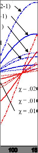
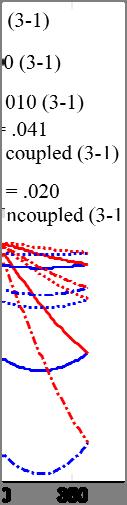
 Here, the non-dimensional parameter χ refers to the separation to wavelength ratio that is the ratio of the separation distance d between two membranes and the wavelength of the sound source.")
35 where (2.17) (2.18) (2.19) Here, the non-dimensional parameter χ refers to the separation to wavelength ratio that is the ratio of the separation distance d between two membranes and the wavelength of the sound source. Ω is the frequency ratio of the excitation frequency ω to the first natural frequency of the system ω 1, is the natural frequency ratio between the bending mode natural frequency and the rocking mode natural frequency, and the ξ, are the damping factors. By taking the ratio of two of the response equations, the transfer functions relating the oscillations of membrane pairs can be derived as The subscript in the transfer functions refers to which two membranes are being compared. For example, the transfer function H 2-1 refers to the transfer function of the oscillations between the membranes 2 and 1. These transfer functions (2.20) (2.21) (2.22) 22
36 can then be used to determine directional cues in terms of the mipd. The mipd can be found as By comparing the phase differences obtained from multiple membrane pairs, the location of the sound source can be determined in two dimensions. (2.23) ( 2.24) (2.25) Numerical simulations of the equilateral triangle configuration Numerical simulations were carried out to analyze the performance of the equilateral triangle configuration. To make the simulation results comparable between configurations, parameters were set at some fixed values and then scaled if it is needed to meet the physical requirements of a specific system. The distance d was selected as d = µm, corresponding to a separation distance of 1225 µm between membrane centers. This distance was selected because it is comparable to that of the fly ear and it is also a feasible distance for micro-fabrication. Note that for the equilateral triangle configuration, the maximum achievable natural ratio is 2, which can only be achieved when k p >> k. Considering to the limitations of microfabrication, this ratio was set to be 1.8 in the simulation. The selected natural frequencies are f 1 = Hz, f 2 = Hz, and f 3 = Hz. Considering a low damping case, the damping factors were selected as ξ 1 = 0.01, ξ 2 = 0.01, and ξ 3 = These selected simulation parameters were kept consistent for the various design configurations to be discussed later. 23


, it can be found that the")
37 First, phase difference as a function of the azimuth angle is plotted at a constant elevation angle, as shown in Figure 2-4. Here, = 90º is selected since at this angle the greatest phase difference can be obtained. The uncoupled case is obtained by considering three separate microphones arranged in an equilateral triangular configuration. As can be seen in Figure 2-4, compared with the uncoupled case, the phase differencee across the entire region of θ, excluding when mipd = 0º, is amplified by a factor of a more than 3 due to the mechanical coupling. Furthermore, if the directional sensitivity is definedd as the derivative of phase difference with respect to an angle of incidence (θ or φ), it can be found that the same amplification of the directional sensitivity can be obtained over the entire range of azimuth. Figure 2-4. Phase difference versus azimuth angle θ obtained from the equilateral triangle configuration. In the simulations, φ is 90 and the excitation frequency is 2 khz. 24


38 2-5. Phase difference versus elevation angle φ obtained from the equilaterall triangle configuration. In the simulations, θ is 30 and the excitation frequency is 2 khz. A linear relationship between the phase difference and azimuth angle can be found between θ = 70º to 120º and 250º to 300º, in which the directional sensitivity is constant. Within this linear region, the localization of a sound source can be easily achieved. In Figure 2-5, phase difference versus elevation angle φ at an excitation frequency of 2 khz is plotted. As expected, all three membranes will oscillate in phase when φ = 0º, resulting in a zero phase difference. When φ = 90º, the maximumm phase difference can be obtained. By dividing the coupled case by the uncoupled case, an amplification factor of above 3 times the uncoupled case is obtained across the entire region of the elevation angle. 25


39 Figure 2-6. Phase difference versus excitation frequency obtained for equilateral triangle configuration. In the simulations, φ = 90 and θ = 30. The same amplification factor is achieved when considering the directional sensitivity of the sensor. As can be seen in Figure 2-5, for the elevation angle range between 0º to 40º, there is a semi-linear region, in which a constant directional sensitivity can be obtained. To understand the performance of the equilateral triangle configuration in terms of the frequency response of mipd, phase difference versus excitation frequency is plotted in Figure 2-6, where φ and θ are held constant at 90º and 30º, respectively. In Figure 2-6, the effects of the rocking and bending mode natural frequencies on the phase difference of the system can be observed. As the excitation frequency 26
40 approaches the rocking mode natural frequency, there is significant amplification of the phase difference. At 9.5 khz, just below the rocking mode natural frequency, the amplification factor as compared to the uncoupled case reaches 11.39, which implies that the performance of this device is comparable to a device which is over 11 times its size. On the other hand, as the excitation frequency approaches the bending mode natural frequency, the phase differences approach zero degrees. This is due to the fact that all three membranes oscillate in phase at the bending mode and no phase difference can be obtained. Through proper selection of device geometry and materials, desired natural frequencies can be obtained, and thus a device based on this configuration can be designed to have desirable performance at select frequency ranges Reduced-order model of the right angle, isosceles configuration Theoretically, using two orthogonally oriented two membrane systems, the sound source can be localized in two dimensions. Based on this idea, a threemembrane device with a right angle, isosceles configuration is proposed here. A reduced-order model of this configuration is illustrated in Figure 2-7. Similar to the previous models, each of the membranes is represented by a mass (m), a spring (k), and a damper (c), which can oscillate due to the pressure gradient of an incident sound source. Each of the coupling beams is considered as subsystem consisting of a torsion spring (k p ) and a damper (c p ). In essence, this configuration represents two orthogonally oriented two-membrane devices that share a common membrane. 27
41 Figure 2-7. Reduced-order model of the right angle, isosceles configuration. Such a system offers the advantage of reducing the complexity of sensing components that are required to detect the deflections of the membranes Analytical solution for the right, isosceles configuration as The governing equations for the right, isosceles configuration can be derived where (2.26) (2.27) (2.28) and (2.29) 28
42 The excitation force vector can be written as (2.30) where a is the area of the membrane, p 0 is the initial pressure, ω is the excitation frequency, d is the separation distance between the membrane s center and the center of the device, and v is the sound speed. The independent variables of θ and φ refer to the azimuth angle and the elevation angle, respectively. Note that the force vector acting on this system is obtained to account for the locations of the membranes relative to the center point of the device, equidistant from each membrane center. By using a similar analysis, the mode shapes and natural frequencies of the system can be obtained as the following: (2.31) (2.32) The first mode appears to be a rocking mode in which one membrane will oscillate 180º out of phase with the other two. However, at the natural frequency corresponding to this mode, the amplitudes of the oscillations of the two membranes are uneven. The mode shape results also indicate a rocking mode at the second natural frequency and a bending mode at the third natural frequency, both of which are similar to those obtained from the equilateral configuration. Based on these natural frequencies, a maximum resonant frequency ratio of 2.4 can be achieved when k p >> k, which is slightly higher that that obtainable from the equilateral configuration, rendering better the amplification of the mipds. 29
43 Through manipulation of the governing equations, the time response of the membranes can be found as: where ( 2.33) (2.34) (2.35) (2.36) (2.37) (2.38) (2.39) and (2.40) (2.41) Here, the non-dimensional parameter χ refers to the separation to wavelength ratio. Ω refers to the frequency ratio between the excitation frequency ω and the first natural frequency of the system ω 1, 1 is the natural ratio between ω 2 and ω 1, 2 is the natural ratio between ω 3 and ω 1, ξ are the damping factors, 1 is the ratio between ξ 2 and ξ 1, and 2 is the ratio between ξ 2 and ξ 1. 30
44 By taking the ratio of two of the response equations, the transfer functions relating the oscillations of membrane pairs can be derived as These transfer functions can then be used to determine directional cues in terms of the mipds, which can be written as: (2.42) (2.43) (2.44) By comparing the phase differences obtained from multiple membrane pairs, the location of the sound source can be determined in two dimensions. (2.45) (2.46) (2.47) Simulation results of the right angle, isosceles configuration In order to keep the simulations comparable to the previous configuration, the distance d was chosen as d = µm, corresponding to a separation distance of 1000 µm between membrane centers. The selected natural frequencies are f 1 = 8311 Hz, f 2 = Hz, and f 3 = Hz. Considering low damping, the damping factors were selected as ξ 1 = 0.01, ξ 2 = 0.012, and ξ 3 = In Figure 2-8, the phase difference is obtained as a function of azimuth angle θ at elevation angle φ = 90º and excitation frequency of 2 khz. As can be seen in this figure, the amplification factor, derived by dividing the coupled case by the uncoupled case, reaches as high as 9.3, 31


45 for mipd 2-1, yet varies at different incident angles. Therefore, despite the high amplification factor, this device may suffer from a lack of uniform directionality. In Figure 2-9, the phase difference is plotted as a function of the elevation angle φ at θ = 30º and excitation frequency of 2 khz, for the same design parameters. Note that at φ = 0 and φ = 90, the minimum ( i. e., 0º) and maximum mipd (provide value) can be obtained, respectively. Also, at θ = 0 and θ = 180º, due to symmetry of the configuration along this azimuth angle mipd 2-1 = mipd 3-1. The amplification factor of this plot reaches as high as 5.9 for both phase difference and directional sensitivity. These simulation results suggest that this design can provide better amplification of the directional cues when compared to the equilateral triangle design. Figure 2-8. Simulation results for right angle, isosceless configuration: phase difference versus θ at φ = 90 and the excitation frequency of 2 khz. 32


46 Figure 2-9. Simulation results for right angle, isosceless configuration: phase difference versus φ at θ = 30 and the excitation frequency of 2 khz. Figure Simulation results for right angle, isosceles configuration: phase difference versuss excitation frequency at φ = 90 and θ =
47 To understand the performance in terms of the frequency response of mipd, phase difference versus excitation frequency is plotted in Figure 2-10, at the incident angles of θ = 30º and φ = 90º, for the same design parameters. As seen in Figure 2-10, this configuration can provide significant amplification of the phase differences at a very limited frequency range. The fluctuation of positive and negative phase differences in certain frequency regions may hinder the device performance in those frequency regions. Therefore, if the sound source frequency is known, a sensor device utilizing this configuration can be designed to significantly amplify the phase difference and directional sensitivity. However, the device may have a very limited operational frequency range. 2.4 Sensor Design with Four Coupled Membranes Introduction Extending further upon the knowledge gained from the two membrane system, a four membrane system is expected to be more than capable of localizing the sound source in multiple dimensions since more phase difference information can be obtained from such a system. This additional information may help improve the accuracy and efficiency of the sound source localization. A better efficiency (i.e, faster localization) can be helpful for localizing a target moving at a high speed. However, the drawbacks of this design include increased sensor size, more sensing components required for signal detection, higher cost, and higher complexity. The analysis performed in the subsequent sections of this chapter will be used to characterize the performance of this system. 34
48 Similar to the three membrane system, there are a number of design configurations to consider for the four membrane device. However, for symmetry and simplicity, the square configuration was selected for further study. This system configuration will be used to study the feasibility of a four membrane device Reduced-order model of the square configuration The reduced-order model of the square configuration is illustrated in Figure In this model, each of the membranes is represented by a mass (m), a spring (k), and a damper (c), which can oscillate due to an incident sound wave. Each of the coupling beams is considered as a subsystem consisting of a torsion spring (k p ) and a damper (c p ). Figure Reduced-order model of the square configuration Analytical solution for the square configuration From the mass-spring-damper system, the underlying governing equation is derived as: 35
 where a is the area of the membrane, p 0 is the initial pressure, ω is the")


49 where (2.48) (2.49) (2.50) and (2.51) The acting force vector is written as (2.52) where a is the area of the membrane, p 0 is the initial pressure, ω is the excitation frequency, d is the separation distance between the membrane s center and the center of the device, and v is the sound speed. The independent variables of θ and φ refer to the azimuth angle and the elevation angle, respectively. In the case of free vibration, the mode shapes and natural frequencies of the system are: (2.53) (2.54) 36

50 The mode shapes indicate that there is a bending mode at the fourth natural frequency, in which all four of the membranes will oscillate in phase. The second and third natural frequencies indicate a rocking mode, in which two of the nonadjacent membranes will oscillate 180º out of phase with each other. The first mode shape is unique in that each adjacent membrane will oscillate 180º with each other. One possible benefit of these three distinct rocking mode natural frequencies is the greater potential of varying the natural frequency ratios. This may prove useful in improving the phase differences and directional sensitivity of the system. Through manipulation of the governing equations, the time response describing the translation of the membranes is derived, which can be written as: where (2.55) (2.56) (2.57) (2.58) (2.59) (2.60) and (2.61) 37
51 (2.62) Here, the non-dimensional parameter χ refers to the separation to wavelength ratio which is the ratio of the separation distance d between microphones and the wavelength of the excitation frequency. Ω refers to the frequency ratio between the excitation frequency ω and the first natural frequency of the system ω 1, 1 is the natural ratio between ω 2 and ω 1, 2 is the natural ratio between ω 4 and ω 1, ξ are the damping factors, 1 is the ratio between ξ 2 and ξ 1, and 2 is the ratio between ξ 4 and ξ 1. Taking the ratio of two of the responses of the membranes, the transfer functions relating the oscillations of microphone pairs are derived as: derived as: Utilizing the transfer functions, the mipds of the four membrane system are (2.63) (2.64) (2.65) (2.66) (2.67) (2.68) 38


52 With the additional mipd information from multiple membrane pairs, the accuracy of the sound localization is expected to improve compared with that of the three- membrane designs Simulation results of the square configuration In the simulation, d is chosen as µ m and the natural frequencies used are f 1 = 5033 Hz, f 2 = Hz, f 3 = Hz, and f 4 = Hz. The damping factors were selected as ξ 1 = 0.01, ξ 2 = 0.026, ξ 3 = 0.026, and ξ 4 = All of thesee parameters are selected so that the results can be comparable to the previously discussed configurations. In Figure 2-12, the phase difference is plotted as a functionn of the azimuth angle θ for the four membrane system. Figure Simulation results for square configuration: phase difference versus θ at φ = 90 and excitation frequency of 2 khz. 39


53 Figure Simulation results for square configuration: phase difference versus φ at θ = 30 and the excitation frequency of 2 khz. Figure Square configuration simulation results: phase difference versus excitation frequency at φ = 90 and θ =
54 Unlike the previous phase difference versus θ plots, where all of the membranes where compared against the first membrane, this plot compares two adjacent membranes, which is useful in analyzing the results. Note that at θ = 45 and θ = 225, it is found that mipd 2-1 = mipd 4-3 = 0º. While at θ = 135 and θ = 315, it can be seen that mipd 3-2 = mipd 1-4 = 0. These results are as expected, which validates that the simulation results are indeed correct. The amplification factor achieved for the phase difference and directional sensitivity is little less than 2. In Figure 2-13, the phase difference is plotted as a function of the elevation angle φ. Similar to the three membrane device, as expected, at φ = 0º, there is a zero phase difference between the membrane pairs, and at φ = 90º, the maximum phase differences are obtained. Compared with that obtained in a three membrane configuration, a lower amplification of the phase differences is apparent. At an excitation frequency of 2 khz, the amplification factor only reaches Therefore, there is a tradeoff between the amplification of the phase difference and the additional phase difference information. In Figure 2-14, the phase difference versus excitation frequency is plotted, which can be used to explain how the amplification factor will change at different operational frequencies. Similar to the equilateral triangle three-membrane configuration, there is a significant amplification of the phase difference in the vicinity of the second and third natural frequencies and no amplification at the fourth natural frequency. These natural frequencies correspond can be adjusted to obtain desired amplification of the phase difference. In the vicinity of the first natural frequency, only slight 41
55 amplification of the phase difference can be achieved. The overall trends show that this amplification obtained from the four membrane system would be less than that is achievable by using the three membrane systems. 2.5 Summary of Designs In this chapter, a wide variety of design considerations were discussed. The analysis of the two membrane system provided a basis for the study of the other systems. In the two membrane system, an incoming sound pressure causes oscillatory movement of the two membranes. Due to the mechanical coupling of the two membranes, the phase difference between the oscillations of the two membranes will be amplified. Since only one phase difference is obtained, it is impossible to realize multi-dimensional sound source localization with such a system. To accomplish the task of multi-dimensional sound source localization, the designs incorporating three or four coupled membranes were developed. In the study of the three membrane and four membrane designs, it was found that each design had its own distinct advantages and disadvantages. The equilateral triangle configuration has a definitive advantage in uniform directionality, while the right angle, isosceles configuration has the advantage of large amplification of the directional cues along very select operational frequency range. The four membrane system is capable of obtaining more phase difference information, which may lead to higher accuracy of the localization results. Unfortunately, there are also inherent limitations in each design. The equilateral triangle system has a limited maximum amplification of the directional cues and directional sensitivity, while the right angle, isosceles device is impaired by 42
56 its non-uniform directionality and limited operational frequency range. Lastly, the four membrane device can realize even less amplification of the phase differences, as compared to the equilateral triangle system. In addition, adding an additional membrane can increase the sensor size and complexity of the sensing components, which will lead to increased cost, power consumption, and weight of the system. In this thesis, the three membrane equilateral triangle system was selected for further investigation due to its simplicity, uniform directionality, sufficient amplification of the phase differences, and broad usable frequency range. 43
57 3 Parametric Study of the Design Parameters 3.1 Introduction A parametric study is presented to understand the effects of varying design parameters on the system performance, in terms of phase differences and directional sensitivity. Directional sensitivity is defined as the change in phase difference with respect to a change in the incident angle. The goal of this study is to obtain appropriate design parameters so that both system performance parameters can be maximized. Improving the amplification of the phase differences would infer that the device can localize a sound source with a similar performance to that of a larger scale uncoupled device. Maximizing directional sensitivity improves the sensors accuracy and resolution in sound source localization estimates. The non-dimensional parameters being studied are natural frequency ratio (η), damping ratio (γ), and separation-to-wavelength ratio (χ). The following parametric study is meant to understand the effects of varying each of these dimensionless design parameters. 3.2 Effects of Natural Frequency Ratio The natural frequency ratio is defined as the ratio between the bending and rocking mode natural frequencies of the system, η = ω 3 /ω 1. Through expansion of the natural frequency ratio to η = ω 3 /ω 1 = where χ k = k p /k is the stiffness ratio, it may be observed that the natural frequency ratio may be adjust by altering the stiffness of the coupling beams relative to the membrane s stiffness. Based on the equation describing the natural frequency ratio, the maximum 44


58 feasible natural frequency ratio of the equilateral triangle device is 2, and the minimum is 1. In the following study, the natural frequency ratio is varied from 1.5, 1.75, to 2. In Figure 3-1, a comparison of phase difference versus θ at a select angle of φ = 90º and excitation frequency of 7 khz is shown. In Figure 3-2, phase difference versus φ at 7 khz excitation frequency and θ = 30º is plotted. In Figure 3-3, phase difference versus excitation frequency is obtained at φ = 90º and θ = 30º. As can be seen in Figures 3-1 to 3-3, the directional cue of phase difference is amplified across the entire region of θ, φ, and excitation frequency for the larger natural frequency ratio of 2, except when mipd = 0. Also, the response improves as the excitation frequency approaches the first natural frequency of the system. Figure 3-1. Natural frequency ratio: phase difference versus θ at φ = 90 and excitation frequency of 7 khz. 45


59 Figure 3-2. Natural frequency ratio: phase difference versus φ at θ = 30 and excitation frequency of 7 khz. Figure 3-3. Natural frequency ratio: phase difference versus excitation frequency at φ = 90 and θ =
60 Although a natural frequency ratio of 2 is infeasible due to material and manufacturing limitations, a larger natural frequency ratio would improve the system responses in terms of phase difference. This can be achieved by altering the stiffness ratio to create a much stiffer coupling beam relative to the membrane. Directional sensitivity is also considered at similar natural frequency ratios. In Figures 3-4, directional sensitivity, dmipd/dθ, versus θ at a select angle of φ = 90º and excitation frequency of 7 khz is presented for different natural frequency ratios. In Figure 3-5, the directional sensitivity, dmipd/dφ, versus φ is plotted at θ = 30 an excitation frequency of 7 khz. In Figures 3-6, directional sensitivity, dmipd/dθ, versus excitation frequency at a select angle of φ = 90º and θ = 90º is shown. In Figure 3-7, the directional sensitivity, dmipd/dφ, versus excitation frequency at φ = 20º and θ = 30º is presented. The results of directional sensitivity at various natural frequency ratios suggest that a higher natural frequency ratio will induce better performance of the device in terms of directional sensitivity. The results also suggest that the amplification will increase as the excitation frequency approaches the first natural frequency of the system. Ultimately, these results conclude that the directional sensitivity is greatly amplified across the entire region of θ and φ, for the larger natural frequency ratio of 2. Since both system responses have a favorable outcome to an increased natural frequency ratio, the system should be designed to have a maximum stiffness ratio between the coupling beams and the membranes. 47


61 Figure 3-4. Natural frequency ratio: directional sensitivity versus θ at φ = 90 and excitation frequency of 7 khz. Figure 3-5. Natural frequency ratio: directional sensitivity versus φ at θ = 30 and excitation frequency of 7 khz. 48


62 Figure 3-6. Natural frequency ratio: directional sensitivity with respect to θ versus excitation frequency at φ = 90 and θ = 90. Figure 3-7. Natural frequency ratio: directional sensitivity with respect to φ versus excitation frequency at φ = 20 and θ =
63 3.3 Effects of Damping Factor Ratio and Damping Factors The damping factor ratio is defined as = ξ 3 /ξ 1 =. The system was set at a low damping factor of ξ 1 =.1 in each of the following cases. In this study the damping factor ratio is varied from 4/7, 1, to 16/7 based on the minimum and maximum limitations of the damping factor ratio equation. In Figure 3-8, the comparison of phase difference versus θ at a select angle of φ = 90º and excitation frequency = 7 khz is presented. Figure 3-9 plots phase difference versus at θ = 30 and an excitation frequency of 7 khz. In Figure 3-10, phase difference versus excitation frequency is plotted at φ = 90º and θ = 30. In Figures 3-11 and 3-12, a comparison of directional sensitivity versus θ and φ respectively at the same design parameters is presented. In Figures 3-13, directional sensitivity, dmipd/dθ, versus excitation frequency at a select angle of φ = 90º and θ = 90º is presented. In Figure 3-14, the directional sensitivity, dmipd/dφ, versus excitation frequency at φ = 20º and θ = 30º is shown. These results show a slight advantage for the higher damping factor ratio of 16/7, however the amplification of the phase differences and directional sensitivity is quite insignificant. Increasing the damping factor ratio improves the amplification of the system responses, however this is not a pertinent design consideration. 50


64 Figure 3-8. Damping factor ratio: phase difference versus θ at φ = 90 and excitation frequency of 7 khz. Figure 3-9. Damping factor ratio: phase difference versus φ at θ = 30 and excitation frequency of 7 khz. 51


65 Figure Damping factor ratio: phase difference versus excitation frequency at φ = 90 and θ = 30. Figure Damping factor ratio: directional sensitivity versus θ at φ = 90 and excitation frequency of 7 khz. 52


66 Figure Damping factor ratio: directional sensitivity versus φ at θ = 30 and excitation frequency of 7 khz. Figure Damping factor ratio: directional sensitivity with respect to θ versus excitation frequency at φ = 90 and θ =


67 Figure Damping factor ratio: directional sensitivity with respect to φ versus excitation frequency at φ = 20 and θ = 30. A more valuable study is to consider the effects of varying the individual damping factors. For this study, the ratio between the two damping factors will be held constantt at 1, allowing both of the damping factors to be vartied from.1,.5, to 1.0. In Figure 3-15, a comparison of phase difference versus θ at a select angle of φ = 90º, excitation frequency of 7 khz, and η = 1.75 is presented. In Figure 3-16, phase difference versus at a select angle of θ = 30º and excitation frequency of 7 khz is compared for different damping factors. In Figure 3-17, phase differencee versus excitation frequency at a select angle of φ = 90º, θ = 30º, and η = 1.75 is obtained for different damping factors. 54


68 Figure Damping factor: phase difference versus θ at φ = 90 and excitation frequency of 7 khz. Figure Damping factor: phase difference versus φ at θ = 30 and excitation frequency of 7 khz. 55


69 Figure Damping factor: phase difference versuss excitation frequency at φ = 90 and θ = 30. The results show that a low damping factor produces much greater phase difference, but there is a sign change in the phase differences occurs at the rocking mode excitation frequency. The abrupt sign change of the phase difference at the rocking mode natural frequency may limit the working freuquency range of the sensor. Thesee results suggest that lower damping factors produce greaterr amplification of the phase differences but limits the usable frequency range. While larger damping factors produce less overall amplification of the phase differences, but is not affected by the abrupt sign change of the phase differences at the rocking mode natural frequency. For further study, in Figure 3-18, directional sensitivity versus θ at a select angle of φ = 90º, an excitation frequency of 7 khz, and η = 1.75 is plotted for 56


70 different damping factors. In Figure 3-19, directional sensitivity versus φ at a select angle of θ = 30º, an excitation frequency of 7 khz, and η = is obtained for the same damping factors. In Figures 3-20, directional sensitivity, dmipd/dθ, versus excitation frequency at a select angle of φ = 90º and θ = 90º is presented. In Figure 3-21, the directional sensitivity, dmipd/dφ, versus excitation frequency at φ = 20º and θ = 30º is shown. These results also suggest that the lower damping factors should be used for increased amplification of the system responses, in terms of phase differences and directional sensitivity. The main drawback of utilizing low damping factors is the abrupt sign change of the phase differences at the first natural frequency of the system. However, this may be overcome by designing a device with a first natural frequency slightly greater than the desiredd operational frequency range. Figure Damping factor: directional sensitivity versus θ at φ = 90 and excitation frequency of 7 khz. 57


71 Figure Damping factor: directional sensitivity versus φ at θ = 30 and excitation frequency of 7 khz. Figure Damping factor: directional sensitivity with respect to θ versus excitation frequency at φ = 90 and θ =


72 Figure Damping factor: directional sensitivity with respect to φ versus excitation frequency at φ = 20 and θ = Effects of Separation-to-Wavelength Ratio The separation-to-wavelength ratio is used to study how the system performance is related to the system size and the wavelength of the excitation frequency. For the purposes of this study the separation-to-wavelength ratio which was previously defined as χ = fd/v, has been redefined to χ = f 1 d/v. This alteration relates the size of the microphone array to a select sound wavelength, rather than the entire operational frequency range. For the previous parametric studies, the design parameters were selected in such a way that the separation-to-wavelength ratio was set at χ 0 = (10 khz * µm)/ 3444 m/s = In this study, the separationby varying to-wavelength ratio is varied from.5χχ 0 = , χ 0, to 2χ 0 = d, in order to further understand its effects. In Figure 3-22, phase difference versus θ 59
73 at a select angle of φ = 90º and excitation frequency of 7 khz is compared for different separation-to-wavelength ratios. In Figure 3-23, a similar comparison of separation-to-wavelength ratios is presented for phase difference versus φ at θ = 30 and an excitation frequency of 7 khz. In Figure 3-24, phase difference versus excitation frequency at φ = 90º and θ = 30 is plotted for different separation-towavelength ratios. These results suggest that a larger separation-to-wavelength ratio will induce greater performance in terms of phase difference across the entire region of θ, φ, and excitation frequency. In Figure 3-25, a comparison of directional sensitivity versus θ at a select angle of φ = 90º and excitation frequency of 7 khz is presented. In Figure 3-26, similar separation-to-wavelength ratios are compared for directional sensitivity versus φ at θ = 30 and an excitation frequency of 7 khz. In Figures 3-27, directional sensitivity, dmipd/dθ, versus excitation frequency at a select angle of φ = 90º and θ = 90º is shown. In Figure 3-28, the directional sensitivity, dmipd/dφ, versus excitation frequency at φ = 20º and θ = 30º is presented. For the results presented in Figures 3-22 to 3-28, the device size changes for both the coupled and uncoupled cases. Since both are changing simultaneously, it is quite difficult to accurately compare the effects of varying this design parameter. To simplify the information being presented, an amplification factor is defined, which is the ratio of the response differences between the coupled and uncoupled devices of similar separation-to-wavelength ratio. In Figure 3-29, a comparison of amplification factor of phase difference versus θ at a select angle of φ = 90º and excitation frequency of 7 khz is shown. 60


74 Figure Separation-to-wavelength ratio: phase difference versus θ at φ = 90 and excitation frequency of 7 khz. Figure Separation-to-wavelength ratio: phase difference versus φ at θ = 30 and excitation frequency of 7 khz. 61


75 Figure Separation-to-wavelength ratio: phase difference versuss excitation frequency at φ = 90 and θ = 30. Figure Separation-to-wavelength ratio: directional sensitivity versus θ at φ = 90 and excitation frequency of 7 khz. 62


76 Figure Separation-to-wavelength ratio: directional sensitivity versus φ at θ = 30 and excitation frequency of 7 khz. Figure Damping factor: directional sensitivity with respect to θ versus excitation frequency at φ = 90 and θ =


77 Figure Damping factor: directional sensitivity with respect to φ versus excitation frequency at φ = 20 and θ = 30. In Figure 3-30, amplification factor of phase difference versus φ at an excitation frequency of 7 khz is compared for different separation-to-wavelength ratios. In Figure 3-31, amplification factor of phase difference versus excitation frequency at φ = 90 and θ = 30 is compared. In Figure 3-32, a comparison of amplification factor of directional sensitivity versus θ at a select angle of φ= 90º is presented. For the same separation-to- wavelength ratios, in Figure 3-33, amplification factor of directional sensitivity versus φ at an excitation frequency of 7 khz is compared. In Figures 3-34, amplification factor of directional sensitivity, dmipd/dθ, versus excitation frequency at a select angle of φ = 90º and θ = 90º is presented. In Figure 3-35, amplification factor of directional sensitivity, dmipd/dφ, versus excitation frequency at φ = 20º and θ = 30º is shown. 64


78 Figure Separation-to-wavelength ratio: amplification factor of phase difference versus θ at φ = 90 and excitation frequency of 7 khz. Figure Separation-to-wavelength ratio: amplification factor of phase difference versus φ at θ = 30 and excitation frequency of 7 khz. 65


79 Figure Separation-to-wavelength ratio: amplification factor of phase difference versus excitation frequency at φ = 90 and θ = 30. Figure Separation-to-wavelength ratio: amplification factor of directional sensitivity versus θ at φ = 90 and excitation frequency of 7 khz. 66


80 Figure Separation-to-wavelength ratio: amplification factor of directional sensitivity versus φ at θ = 30 and excitation frequency of 7 khz. Figure Separation-to- wavelength ratio: amplification factor of directional sensitivity with respect to θ versus excitation frequency at φ = 90 and θ =

81 3-35. Separation-to-wavelength ratio: amplification factor of directional sensitivity with respect to φ versus excitation frequency at φ = 20 and θ = 30. From Figures to 3-28, it can be seen that the larger separation-to- wavelength ratio corresponds to greater phase differences and directional sensitivities. However, based on Figures 3-29 to 3-35, the performance parameters are better amplified by using the system with a smaller separation-to-wavelength ratio. This indicates thatt a system with a larger separation-to-wavelength ratio between the membranes will have greater directional cues as well as directional sensitivity. However, the overall performance gain over an uncoupled counterpart of similar size is less compared with a system with a smaller separation-to-wavelength ratio. These results show the importance of applying the coupling system for the small-scale devices. As the size of the device is reduced, the relative device performance improves. On the other hand, increasing the first natural frequency of the device willl 68
82 induce similar results. Best performance gain due to the coupling may arise from a small device with a large first natural frequency. 3.5 Summary In this chapter, parametric studies were carried out to fully comprehend the effects of four dimensionless design parameters on the system performance. The study of natural frequency ratio suggests that increasing the natural frequency ratio increases the amplification of the phase differences and the directional sensitivity. To produce a high natural frequency ratio the coupling beam should be designed for a much greater stiffness than the corresponding membranes. The study into the effects of the damping factor ratio suggests that a greater damping factor ratio would be relatively beneficial to the system performance. However, such effects are not significant. More importantly, varying the individual damping factors of the system can induce a greater effect on the system performance. Low damping factors can help improve the amplification factor of both phase difference and directional sensitivity, but limit the operational frequency range of the system. While high damping factors produce less amplification of the phase difference and directional sensitivity, but they can help improve the frequency range for which the system can operate. The study into the effects separation-to-wavelength ratio suggests how the system performance will be affected by alterations of the device size and first natural frequency. These results show that as the device size is increased, the phase differences and directional sensitivity are also increased. However, an increased device size reduces the relative advantage of the coupled system over the uncoupled 69
83 system. This study is useful in finding the common ground between useful levels of performance metrics and adequate amplification of the metrics. In device design, the device size can first be selected and then the first natural frequency of the system can be adjusted until the desired system performance is obtained. In conclusion, the results from the parametric studies can be used as a guide to further the development of bio-inspired sound localization sensors. The knowledge gained from these studies is applied during the design for fabrication process to obtain sound sensor devices with more desirable performance. 70
84 4 Development of Sensor Device and Sensor Signal Detection System 4.1 Introduction As discussed in Chapter 2, a three-membrane equilateral triangle configuration has been selected for further investigation. In this Chapter, development of a sensor device with such a configuration will be discussed. The sensor is fabricated by using micro-electro-mechanical system (MEM) methods. Furthermore, a fiber-optic interferrometric sensing system will be described, which is used to detect the sound induced membrane deflections. This system makes use of a Fabry-Perot interferometer which is formed between the backside of the diaphragms and the end-face of the optical fibers. The Fabry-Perot interferrometric sensing technique provides an approach for accurate detection of the membrane deflections yet does not impact the structure dynamics of the membranes or coupling beams. 4.2 Development of the Sensor Device The sensor device includes two bonded layers. The first layer of the device, known as the sensing head component, consists of the three membranes, the coupling beams, and the respective anchors and pivots. The second layer, known as the optical fiber guide, provides alignment holes that are used to guide and secure the optical fibers at the appropriate distance relative to the back side of the membranes. These two layers are later aligned with each other and bonded using a thermal adhesive. Once aligned and bonded, the optical fibers are then inserted and secured at the select operating distance using an ultraviolet curable epoxy. The schematic of a fully assembled sensor device is shown in Figure
85 Figure 4-1. Schematic of fly-ear inspired sound localization sensor: (a) overview and (b) cross- section view. The optical fibers protruding from the reverse side of the device connect with the rest of the sensing system, which will be described in Chapter 5. The following sections of Chapter 4 willl discuss the MEMS fabrication process of the sensing head and fiber guide components, along with the assembly of the device and the insertion of the optical fibers Fabricating the sensing head component MEMS processes were used for fabrication of the micro-scale sensor device. The MEMS fabrication process is illustrated in Figure 4-2. A 250 μm thick double sided polished wafer provides a basiss for manufacturing of these devices. First, a 1 μm layer of silicon dioxide is deposited on the top surface of the polished wafer by using plasma-enhanced chemical vapor deposition (PECVD). This layer acts as an etch stop when etching out the membrane cavities. A 0.5 μmm layer of amorphous silicon is then sputtered on top, whichh later forms the membranes of the device. 72


.")


86 Figure 4-2. Schematic of the MEMS fabrication process used for creating the sensing head component. A sacrificial layer of photoresist is then applied and patterned using a mask and ultraviolet light. This mask is used to define the anchor locations which will connect the coupling beams to the substrate and membranes. Next, the coupling beams are deposited and patterned via reactive ion etching in alternating layers of PECVD silicon dioxide and silicon nitride, to an ultimate thickness of 3 µm. From the backside of the silicon wafer, the membranes are patterned and etched using deep reactive ion etching (DRIE). The first layer of silicon dioxide acts as an etch stop to prevent the DRIE from removing the membrane surfaces. Reactive ion etching is then used to remove the layer of silicon dioxide, blocking the underside of the membranes. The die is then cleaved to allow separation of the individual sensing head components. Finally, the sacrificial photoresist is removed in an isotropic oxygen plasma etcher. 73
 SEM image of the microfabricated sensor device and (b) a microscope image of the")


87 (a) (b) Figure 4-3. (a) SEM image of the microfabricated sensor device and (b) a microscope image of the microfabricated device. A fabricated sensor head component is shown in Figure 4-3. The average dimensions for a fabricated device are as follows: membrane thickness of 0.5μm, radius of 575μm, and coupling beam dimensions of 1200μm 300μm 3μm. To adjust the device performance, the length and width of the coupling beam, along with the radius of the membranes can be varied by as much as +/-50µm. Similar to the sensing head component, the fiber guide is also fabricated by using MEMS processes. This component has a simple design consisting of only three through holes for guidingg the optical fibers to the back side of each of the membranes. Starting with a 250 µm thick double-sided polished wafer, a bond layer of Protek A22 is spun on the top side. The wafer is then patterned for the three through holes and etched from the backside using DRIE. The bond layer acts as an etch stop, but is later removed along the through holes using reactive ion etching in an oxygen plasma. The die is then cleaved and separated for each individual device. The MEMS fabrication process used to create the fiber guide layer is shown in Figure


88 Figure 4-4. Schematic of the MEMS fabrication process used for creating the fiber guide layer Integration of the sensing head and fiber guides The Protek A22 on the fiber guide layer provides adhesion to bond the fiber guides with the sensing head component. A schematic of an appropriately bonded device is illustrated in Figure 4-5. Before bonding, to ensure an appropriate alignment, the two layers are stacked together under a microscope with illumination from both the top and bottom of the device. The backside illumination allows one to see the alignment holes of the fiber guide throughh the silicon membranes. Tweezers are used to align the through holes of the fiber guide to the centers of the membranes, where the coupling beams are anchored to the membranes. Once aligned, the two layers can be bondedd together through heating with a hot plate, at 200 C for three minutes. Figure 4-5. Schematic of the assembled sensor device. 75
89 4.2.3 Assembling optical fibers to sensor device To detect the minute deflections of the membranes, fiber optic Fabry-Perot interferometers are used, which are constructed between the end faces of optical fibers and the membranes of the sensor. To obtain these interferometers, the alignment of optical fibers to the backside of the membranes and bonding them at a fixed distance is necessary. In the alignment process, a selected device is first secured to the specialized mount via a piece of double-sided tape. This mount allows for access to the backside of the sensor device, so that the optical fibers can be aligned and secured. The double-sided tape provides a strong, yet temporary attachment of the device to the mount, which can be removed when the assembly process is finished. A fiber holder is used for positioning the optical fiber. Two three-axis translational stages are used to provide sufficient flexibility and accuracy for aligning the optical fibers with the through holes on the fiber guide. An image of a device on the mount during the assembly process is shown in Figure 4-6. A cleaved optical fiber is then inserted into the fiber holder and secured with the tape. The other end of the fiber is connected to an optical detection system, which detects the exact position of the fiber end face relative to the sensor membrane so that appropriate positioning of the fiber can be achieved. The optical detection system is depicted in Figure 4-7. In this system, broadband light source is produced by the optical sensing interrogator, sm130 by Micron Optics, is delivered via a 2 1 coupler to the backside of the sensor. The reflected light from the sensor device is then recorded by using the optical sensing interrogator. 76


90 Figure 4-6. Picture of a device during the assembly process in which the optical fibers are inserted and bonded to the system. Figure 4-7. Schematic view of the optical detection system used for fiber alignment. This optical system measures the optical spectrum which is used to accurately determine the cavity length between the fiber end face and the backside of the membrane. With this system, the optical fibers can be positioned to obtain the exact 77


91 Fabry-Perot cavity length required by the optical sensing system (~60 µm), which will be discussed in the next section. Once the desired Fabry-Perot cavity length is obtained, a small droplet of epoxy is applied and cured using ultraviolet light. The curing process causes a smalll amount of shrinkage, which can be compensated by preemptively setting the cavity length to µm before curing. The slight error in the final cavity length can be further corrected by adjusting the cavity length of the reference interferometer in the optical sensing system to be discussed later. Once the entire device has been assembled, additional epoxy is applied to the back side of the fiber guide to effectively secure the fibers and prevent fractures. A picture of a fully assembled device is provided in Figure 4-8. Figure 4-8. Photographs of a fully assembled device. 78
92 4.3 Fiber Optic Detection System In order to detect the minute deflections of the membranes, many different displacement detection techniques can be used, which primarily include optical or electrical techniques. An electrical detection system can be based on capacitive, piezoelectric, or piezoresistive techniques. A traditional capacitive system utilizes the change in distance between two capacitive plates: one being the membrane of the device and the other being a stationary plate directly behind the membrane. As mentioned in Chapter 1, a comb finger system that uses capacitive fingers protruding around the circumference of the membranes can also be used to detect membrane deflections. However, a major drawback of the capacitive techniques is that the motion of the membranes is inherently resisted. In addition, squeeze film damping needs to be addressed in such a system. This may be detrimental to obtaining accurate membrane deflections and phase differences between them. Another electrical technique is using a piezoelectric or piezoresistive sensing technique. In these systems, a piezoelectric or piezoresistive material is embedded into the membranes, and will deform as the membranes deflect. This deformation can be directly related to a change in electric potential or resistance. However, since the piezoelectric or piezoresistive material is embedded directly into the membranes of the system, the dynamical characteristics of the membrane will be altered, which will affect the performance of the sensor device. 79


93 Figure 4-9. Schematicc of the low coherence fiber optic Fabry-Perot optical detection systems offer interferometer. Compared with their electrical counterparts, great potential for detecting the membrane deflections. Most of these systems rely on some form of interferometry. These systems have the advantage of not being affected by electromagnetic interference, low cost, light weight, robustness in hazardous environments, and that they do not have to come in direct contact with the membranes. In this thesis work, a low coherence fiber optic Fabry-Perot interferometric system is selected and used to detect the membrane deflections. The schematic of this system is illustrated in Figure 4-9. Typical fiber optic interferometers measure the intensity output as: where (4.1) (4.2) 80
94 I 0 is the dc component of the intensity. The variables Φ s and Φ r are the optical phase of the sensing and reference interferometers, and V is the visibility, which is determined by the maximum and minimum values of intensity. In this system, the sensing interferometer is formed between the optical fiber end face and the back side of a membrane. The reference interferometer is accomplished by utilizing a Fabry-Perot tunable filter, which can be adjusted to match the cavity length of the sensing interferometer. This adjustment allows for obtaining a differential cavity length that is much shorter than the coherence length of the light source, and thus, a good visibility of interference can be realized. In this low coherence fiber optic interferometric system, the differential change in optical path length between the sensing and reference interferometers is detected. In order to detect the optical path difference in this system, the cavity length of the sensing interferometer, L s, should be greater than the coherence length, L c, of the light source and must satisfy the following equation: If these conditions are satisfied, the measured light intensity can be approximated as: (4.3) By measuring the differential optical phase change, this system produces a high signal-to-noise ratio, low drift, and allows for a large bandwidth. (4.4) 81
95 5 Experimental Study of the Bio-inspired Sound Localization Sensor System. 5.1 Introduction To characterize the sensor system performance and validate the theoretical analysis of the sound localization sensor, experimental study of the sensor system is carried out. Two types of experimental characterization will be described in this chapter. One is conducted by using a scanning laser vibrometer to measure the natural frequencies and mode shapes of the devices. This device characterization can help validate the presence of both the rocking and bending modes, and obtain the natural frequencies and the resonant frequency ratio of the system, which will be useful in validating the analytical solutions. The second type of characterization is carried out by using the optical sensing system described in Chapter 4, which can help understand the performance of the device with respect to sound incident angles and at different excitation frequencies. The results from these studies will also be discussed. 5.2 Experimental Study of Dynamical Behavior of the Sensor Devices with Scanning Laser Vibrometer A scanning laser vibrometer is used characterized the vibrational modes of the sensor devices before and after the optical fibers are assembled. The preliminary testing prevents the assembly of undesirable devices, while the secondary testing validates the performance of the fabricated devices. The observed natural frequencies may shift during the assembly process, and thus the secondary testing can help ensure 82
 is used to measuree the velocities at select node points on a device.")


96 that the presence of the rocking and bending modes for a chosen device and that theree is a sufficient resonant frequency ratio. In the experiment, a scanning laser vibrometer (PSV-400, Polytec) is used to measuree the velocities at select node points on a device. A speaker (Heil AMT-1 Tweeter, ESS) is used to play a pseudo-random noise ranging from 10-50,000 Hz, which will excite the membranes of the sensor. Once the scan is complete, the response of the membranes at each excitation frequency can be observed. Figure 5-1 shows a set of devices whichh are being tested and Figure 5-2 shows the system with a scan in progress. The first step in the scanning process is focusing and alignment of the device in the viewing area of the scanning vibrometer. The device is aligned with either the top pointing towards or away from the speaker. Figure 5-1. Group of devices being examined using the scanning vibrometer (PSV-400, Polytec) ). 83


97 Figure 5-2. Image of a device being scanned by the scanning vibrometer. Node points are then defined on the sample for scanning, and the laser is calibrated with the surface of the device. Options are selected such that the system will scan each node point three times and take an average. Upon a complete scan through all of the defined node points, the results are analyzed by using the software provided by Polytec. The scanning process is repeated once the devices are fully assembled. The secondary scan ensures the presence of both rocking and bending modes and characterizes the device performance in terms of the natural frequency ratio. Figure 5-3 shows a device being rescanned after the assembly process. Figure 5-3. A device being rescanned after being assembled with the optical fibers. 84


98 5.3 Results Obtained by Using Scanning Laser Vibrometer The results obtained from the scanning laser vibrometer can be used to characterize the dynamical behavior of the devicee and to compare with the results obtained from the simulations. Typical results of the fabricated devices confirm a resonant frequency ratio between 1.4 and 1.7, with a first natural frequency ranging from 10 khz to 20 khz. These results vary based on the beam and membrane dimensions of the device being tested. Two devices with resonant frequency ratios of 1.76 and 1.64, respectively, are selected for further characterization and the experimental results are presented and discussed in this chapter. The frequency response curve obtained by using the scanning laser vibrometer from the first device is presented in Figure 5-4, with a rocking mode natural frequency of 11.3 khz and a bending mode natural frequency of 19.9 khz. The mode shapes of the rocking and bending modes are shown in the inset of Figure 5-4. Figure 5-4. Scanning vibrometer results of the first tested device. 85


99 Figure 5-5. Scanning vibrometer results of the second tested device. The second devicee has a slightly lower resonant frequency ratio, yet it has a higher first natural frequency. The frequency response obtained with the scanning vibrometer is presented in Figure 5-5, with a rocking mode natural frequency of 15.1 khz and a bending natural frequency of 25.1 khz. With the same relative devicee size and a greater first natural frequency, second devicee has a larger separation-to-wavelength ratio compared with the first device. Ultimately, both devices were selected due to their high resonant frequency ratio and distinct rocking and bending modes. 5.4 Experimental Arrangement for Characterization of Device Performance To characterize the performance of a fully assembled device the device, a specialized mount was manufactured, which can make the device accessible to any incident azimuth and elevation angle of a sound source. 86

100 Figure 5-6. Image of the mounting system used to test the device at the full range of incident azimuth and elevation angles. This mount is arranged so that the sensor is located along the central axis of two perpendicular rotational stages. This allows for directly adjusting the azimuth and elevation angles of the incident sound source. Figure 5-6 provides an image of the mount which incorporates both rotational stages. The bottom motorized rotational stage (URS75BPP, Newport) is used to accurately move the sensor device relative to the elevation angle. This stage is controlled via a Universal Motion Controller (Model ESP300, Newport). A LabVIEW program is used to rotate the stage, facilitating the sweeping of the sensor device through all of the tested elevation angles. The same LabVIEW program is used to produce sound at a select excitation frequency through a speaker (AMT-1 Tweeter, ESS Heil). This speaker is placed a predetermined distance in front of the sensor, such that the mount can cover all of the incident angles relative to the speaker. An audio receiver (STR-DH100, Sony) is used to amplify the sound produced by the speaker. The experimental setup with the mount and the speaker is shown in Figure


101 Figure 5-7. Image of the experimental setup of speaker and mount. Figure 5-8. Schematic of the fiber-optic interferomtric detection system. An low coherencee interferometer based fiber optical detection system was developed for obtaining the sensor signal. The schematic of the system is shown in Figure 5-8. A broadband, 1317 nm wavelength, super luminescent light emitting diode is used as the light source for the Fabry-Perot interferometers. The light from this light source is equally split into three paths, each of which is delivered to a sensor 88
102 membrane via a 2x1 coupler. The cavity formed between the optical fiber end face and the membrane acts as a sensing Fabry-Perot interferometer. Three tunable Fabry- Perot filters (FFP-TF2, Micron Optics) are used as reference interferometers. The reference tunable filters can help reduce the effects of noise and miss-calibration. The reflected light is measured using three InGaAs photodectors (Model 2011, New Focus). The electrical output from the photodetectors is monitored in real time through an oscilloscope (Tektronix 2225, Agilent). The output signals are also recorded by using a data acquisition card (NI-USB-6259, National Instruments) for further processing. A laptop computer is used to save the data and control the entire experimental process through the LabVIEW program. In the experimental preparation stage, the cavity lengths of the reference Fabry-Perot tunable filters are first adjusted to match those of the sensor interferometers. Next, the misalignment of the sensor relative to the speaker location is adjusted. Finally, a sample test run is conducted to ensure that the LabVIEW program is working properly. In the experiment, an incident azimuth angle is first selected and the automated testing begins. The signal response from the membranes is sampled at a sampling frequency of 300 khz, and the voltage data is recorded for all three membranes. This data is processed and analyzed by using MATLAB software, which are also compared with the simulation data. The sensor device is moved to obtain sweeping of the incident elevation angles at a varying increment of 5 to 10 (an increment of 5 is used between φ = 30º to φ = 0º to obtain enough data for better characterization of the quasi-linear region of the device). The device performance 89


103 with respect to a changingg azimuth angle is characterized by moving device along the azimuth angle with increments of 30. To obtain the frequency response of the phase differences, the excitation frequency is swept from 1 khz to a frequency just above the bending mode natural frequency of the devicee at an increment of 1 khz. All of measurements are repeated a minimum of three times to ensure accurate data collection and to remove outliers. 5.5 Phase Difference e versus Azimuth Angle Both of the devices presented in Section 5.3 were characterized at a broad range of incident angles and excitation frequencies. The experimental results obtained from Device 1 have been reported in reference [16], which are presented in the appendices of the thesis. In the following sections, the experimental results obtained from Device 2 will be presented and discussed. Figure 5-9. Phase difference versuss θ at φ = 50 and excitation frequency of 2 khz. 90


104 Figure 5-9 plots the phase difference versus the azimuth angle at 2 khz excitation frequency for the experimentally obtained results, the comparative simulation results, and the uncoupled case of a similar size and layout. As can be seen in Figure 5-9, the experimental resultss compare well to the simulation data. Even through the sound frequency of 2kHz is well below that of the rocking mode natural frequency of the system, the results indicate an amplification factor of a little above 2.5 across the entire region of θ, except for those azimuth angles at which the obtained mipd is 0º. These results demonstrate the effectivenesss of this design. To achieve better amplification of the phase differences, the phase difference versus the azimuth angle is also obtained for an operational frequency of 6 khz, closer to that of the rocking mode natural frequency, as shown in Figure At this frequency, an amplification factor of about 3.5 is achieved. Figure Phase difference versus θ at φ = 50 and excitation frequency of 6 khz. 91
105 The experimental results again compare well to the simulation results. One noticeable trend in Figures 5-9 and 5-10 is that the experimental data appears to match the simulation results better along the linear regions of the phase difference versus θ curves, rather than at the peak values of the phase differences. This suggests that performing sound source localization across the linear regions of the curve may produce more accurate localization estimates. 5.6 Phase Difference versus Elevation Angle The phase difference versus the elevation angle at an excitation frequency of 2 khz is shown Figure As expected, a maximum phase difference is obtained at φ = 90, and zero relative phase difference at φ = 0. The experimental results match well with the simulation data. An amplification factor of about 2.7 is apparent in these results across the entire range of the elevation angles. A better correlation of the experimental results to simulation data can be observed along the linear regions of the curves, i.e. from φ =0º to φ =60º. These results suggest that the sensor will be more accurate when it is used for localizing the sound source at or below an elevation angle of 40. In Figure 5-12, the phase difference versus elevation angle is obtained at a higher excitation frequency of 6 khz for a fixed azimuth angle of 150. These results confirm that the amplification factor increases as the excitation frequency approaches the rocking mode natural frequency of the device, roughly from 2.7 to 2.9. However, there still appears to be the same adverse effect that as the excitation frequency approaches the first natural frequency, the discrepancy of the experimental results from simulation data increases. 92


106 Figure Phase difference versus φ at θ = 90 and excitation frequency of 2 khz. Figure Phase difference versuss φ at θ = 150 and excitation frequency of 6 khz. 93


 of the sensor device, and the phase differences shift signs at this frequency due to the low damping of the")
107 5.7 Phase Difference e versus Excitation Frequency The results of phase difference versus excitation frequency are meant to show the effects of the rocking and bending mode natural frequencies on phase differences obtained from the experiments and simulations. In Figure 5-13, phase differences are plotted as a function of the excitation frequency at an azimuth angle of 330 and an elevation angle of 70. As expected, the amplification of the phase differences increases as the excitation frequency approaches the rocking mode natural frequency (15.1 khz) of the sensor device, and the phase differences shift signs at this frequency due to the low damping of the system. Also, beyond the rocking mode natural frequency, the relative amplification factor begins to decreasee as the excitation frequency approaches the bending mode natural frequency of the device. Figure Phase difference versus excitation frequency at θ = 330 and φ =
108 At the bending mode (25.1 khz), all three membranes will oscillate in phase and the obtained relative phase difference is zero. Overall, the simulation data correspond well with the experimental results. However, there does appear to be a larger discrepancy between the experimental and simulated results at a frequency range around the rocking mode. These results suggest that the sensor device can be used to accurately locate a sound source between the excitation frequencies of 1 to 12 khz. 5.8 Summary In the chapter, experimental study of the sound localization sensor system is carried out. First, a scanning laser vibrometer was used to study the dynamical behavior of the fabricated sensor devices and identify the rocking and bending modes of the devices. Further, a fiber optic interferometric detection system was developed and used in characterization of the sensor performance in terms of phase differences at a range of incident angles and excitation frequencies. Overall, the experimental results show significant amplification of the phase differences when compared to an uncoupled microphone array of a similar size and layout. The results also show that the amplification of phase differences increases as the excitation frequency approaches the rocking mode natural frequency of the device and the working frequency of the sensor can be selected over a broad range of frequencies. A good correlation between the simulation and experimental results were observed, which indicates that the simulation results are useful for the development of a sound source localization scheme. The linear regions with less comparable error should be ideal for accurately locating the sound source in two dimensions. The 95
109 amplification achieved from the experimental results indicates that these devices should have a comparable performance to an uncoupled microphone array of three to four times its size. These experimental results demonstrate the effectiveness of applying the mechanical coupling mechanism in the equilateral triangle design, and validate the analytical model developed in Chapter 2. 96
110 6 Localization Scheme 6.1 Introduction The experimental results confirmed that the sensor could differentiate between changes in the azimuth and elevation angles. This information implies that the sensor is capable for two-dimensional sound source localization. To best use the fly-ear inspired sound localization sensor, two different localization schemes are developed for robotic sound source localization. The first scheme is based on a mapping technique, in which the obtained experimental results are compared to a theoretical map of the expected phase differences. This technique is quite accurate but requires significant processing power to create the simulated map and to compare the experimental results. The second scheme is meant to limit the processing power and reduce the time needed for performing localization. This scheme is labeled as a perception based approach, since it utilizes the expected trends to localize the sound source through guess work. In this technique, a simulated map is not necessary, but the overall trends of the simulated data are utilized to train the system as to which direction to turn. 6.2 Mapping Technique A mapping localization technique utilizes processing of the experimental data for obtaining the location of the sound source [17]. By comparing experimentally obtained results to the simulation data, a two dimension map of how the device will react under different incident angles was produced. Through use of the theoretical map, localization of the sound source in two dimensions can be achieved by using the following equation: 97
, the corresponding azimuth and elevation angles are obtained as the most probable location of the incident sound source.")
, the estimated sound source localization in terms of the azimuth and elevation angles can be obtained.")
111 (6.1) The above equation compares the experimentally obtained phase differences to the map of all of the theoretically possible phase difference combinations to find the best match where Sol(θ,φ,ω) is at a minimum. At this local minimum of Sol(θ,φ,ω), the corresponding azimuth and elevation angles are obtained as the most probable location of the incident sound source. To study the performance of this technique, the experimentally obtained mipd data from Device 1 at 2 khz is used to compare with the theoretical map generated based on the simulated results to the obtained experimental results for the same device. Based on Equation (6.1), the estimated sound source localization in terms of the azimuth and elevation angles can be obtained. By comparing these estimated sound locations with true values, the errors in determination of both azimuth and elevation angles at 2 khz can be obtained, which is plotted in Figure 6-1. (a) (b) Figure 6-1. Sound localization error using mapping technique: (a) error in determination of the azimuth angle and (b) error in the determination of the elevation angle. The experimental data obtained with Device 1 at 2 khz was used. 98
112 Figure 6-1 (a) provides a map of the error in the θ estimate for given incident angles of θ and φ, while (b) provides a map of the error in the φ estimates. These maps display which regions of θ and φ will have the greatest error in sound source localization estimates. These results confirm a viable working region between φ = 0º and 40º and across the entire range of θ. At these angles there is relatively low error in the sound source localization results. The error in θ at the angle of φ = 0º was ignored because if φ = 0º the sound source is directly in front of the device and the directional cue of theta is irrelevant. It should be noted that there is some ambiguity in determination of the elevation angle; the mapping method fails to discern whether an incident sound is coming from in front of or behind the sound sensor. This is due to the fact that two solutions of the elevation angle are possible, φ and 180º - φ. If the sound localization sensor is equipped on a moving platform (such as a maneuverable micro air vehicle), multiple iterations of the localization schemes can be performed to overcome the ambiguity. Considering the case of a fixed sound source, the following process can be used for unambiguously localizing a source in two dimensions: i. Take a measurement of phase differences ii. Subtract the zero-offset iii. Determine the azimuth and elevation angles based on the mapping technique iv. Rotate the sensor in the elevation direction at the measured azimuth angle based on the following criteria: a. If φ is between 80º-90º, rotate 50º in the elevation direction b. If φ is between 40º-80º, rotate 40º in the elevation direction c. If φ is between 4º-40º, rotate the full amount of the elevation angle 99
113 d. If φ is between 0º-4º on the 1 st measurement, rotate -20º in the elevation direction e. If φ is between 0º-4º, stop iterations v. Rotate the sensor in the azimuth direction by (260º θ) vi. Repeat steps i-v until φ is less than 4º Depending on the initial location of the incident sound source, this process may have to repeat multiple times to get accurate localization results, especially if the sound source is located at an elevation angle beyond 90º where ambiguity occurs. This localization technique can be revised to reduce the effects of this ambiguity by incorporating the following process: i. Take a measurement of the phase difference ii. iii. iv. Subtract the zero-offset Determine the azimuth and elevation angles based on the mapping technique Rotate the sensor in the elevation direction at the measured azimuth angle based on the following criteria: a. If φ is between 80º-90º, rotate 50º in the φ direction b. If φ is between 40º-80º, rotate 40º in the φ direction c. If φ is between 4º-40º, rotate the full amount of elevation angle d. If φ is between 0º-4º on the 1 st measurement, rotate -20º in the φ direction e. If φ is between 0º-4º, stop iterations v. Rotate the sensor in the theta direction by (260º θ) vi. vii. Repeat steps i-iii If the new elevation angle is greater than the previously obtained value 100
 Else c.")


: (a) original")
114 a. Rotate 90º in the φ direction at the measured azimuth angle b. Rotate the sensor in the azimuth direction by (260º θ) Else c. Repeat steps i-v until the measured φ reaches a value smaller than 4º Following this localization technique, a maximum of five iterations will be required for accurate sound source localization, even when the sound source is originally located behind the sound localization sensor. In Figure 6-2, a visual representation of how this localization technique works is presented and described. φ = 90º (a) (b) (c) (d) Figure 6-2. Sound source localization (star marks location of the sound source relative to the sensor): (a) original location of the source relative to the sensor, (b) location after first iteration, (c) location after the second iteration, (d) final location of the source relative to the sensor. 101
115 In this example, the source is initially located behind the sensor, where θ = 156º and φ = 128º. This location lies in a region of high error and in a region which is beyond φ = 90º. Using the mapping technique, the estimated sound source location is θ = 153.6º and φ = 89.5º. Based on these readings, by applying the localization technique discussed previously, at the first iteration, the sensor will be moved 106.4º in the θ direction and -50º in the φ direction, rendering a sensor location of θ = 262.4º and φ = 78º relative to the source, as seen in Figure 6-2 (b). At the second iteration, the estimated incident angle values are θ = º and φ = 88.61º, and the sensor will be moved -3.56º in the θ direction and -50º in the φ direction. In Figure 6-2 (c), the sound source is now at θ = º and φ = 28º, the sensor reads θ = º and φ = 29.93º, and the sensor will move 1.35º in the theta direction and º in the phi direction. At the final location, Figure 6-2 (d), the sound source is at θ = 80.19º and φ = 1.93º, the sensor reads θ = º and φ = 3.47º and will stop moving. By using this localization technique with the sound localization sensor, localization of a sound source within an accuracy of 2º can be achieved, even though there is large error in estimating the initial location of the source. 6.3 Perception Based Approach The perception based approach is quite different from the mapping technique, in which no processing of the data is required. This technique is adapted from a random guesswork technique, in which the sensor will be continuously moved through all of the incident angles until the phase difference between all three membranes is 0º. This implies that the sensor is pointing directly at or away from the sound source. 102


116 Figure 6-3. Simulation results: Phase difference versus θ. Although this technique will eventually localize the sound source, it is highly inefficient. To improve upon the random guesswork technique, the theoretical prediction of phase difference as a function of azimuth and elevation angles is utilized to guide the movement of the sensor. In Figure 6-3, the simulation results obtained for the three membrane device are presented. Here, only the trends of the curves are used. The first goal is to rotate the sensor to 0 azimuth in the least amount of iterations. Based on trends of the simulated curves, if mipd 2-1 < mipd 3-1 (mipd 2-3 is negative), this suggests that the sensor should be rotated in the negative azimuth direction to reach 0 azimuth in the least amount of iterations. 103
117 Figure 6-4. Simulation Results: Phase difference versus φ. If mipd 2-1 > mipd 3-1 (mipd 2-3 is positive), this implies that the sensor should be rotated in the positive azimuth direction to reach 0 azimuth in the least amount of iterations. Also the difference between mipd 2-1 and mipd 3-1 (mipd 2-3 ) may be utilized to adjust the step size of the iteration. As the system approaches 0º azimuth, the differencee between mipd 2-1 and mipd 3-1 (mipd 2-3 ) will be reduced, and thus the step size between iterations should be reduced to prevent over shoot of the sound source location. Once 0º azimuth is obtained, the next objective is to rotate the sensor towards 0º elevation, at which the device will be perpendicular to or pointing at the sound source. Figure 6-4 plots simulation results of phase difference versus elevation angle, which is used to describe the expected trends. 104


118 Reducing the elevation angle to 0º can be accomplished by moving the sensor in the negative φ direction until 0 phase difference is obtained for mipd 2-1 and mipd 3-1. The step size of each iteration is adjusted based on the value of mipd 2-1 and mipd 3-1 as to not overshoot the sound source location. Once the phase difference between all three membranes is 0, the sound sensor will be pointing directly at the sound source location. Following this localization technique, accurate sound source localization can be achieved, but with more iterations than the mapping technique. In Figure 6-5, an illustration of how this localization technique works is presented and described, starting with localization in the θ direction. Figure 6-5. Sound source localization in the azimuth direction using the perception based approach. 105


119 Table 6-1. Iterations of the perception based approach localizing the sound source localization in the azimuth direction. Iteration Azimuth Elevation mipd21 mipd31 (mipd31- mipd21) In this example, the sound source is initially located at θ = 120º and φ = 70º. This localization technique will follow the iterations listed in Table 6-1 until mipd 2-1 equals mipd Figure 6-6. Sound source localization in the elevation direction using the perception based approach. 106
Available online at ScienceDirect. Procedia Engineering 120 (2015 ) EUROSENSORS 2015
 EUROSENSORS 2015") Available online at www.sciencedirect.com ScienceDirect Procedia Engineering 120 (2015 ) 289 293 EUROSENSORS 2015 Bio-inspired sound localization sensor with high directional sensitivity Andrew Reid a
Available online at www.sciencedirect.com ScienceDirect Procedia Engineering 120 (2015 ) 289 293 EUROSENSORS 2015 Bio-inspired sound localization sensor with high directional sensitivity Andrew Reid a
A ccurate estimation of sound-source location facilitates communication, finding prey, and escape from
 OPEN SUBJECT AREAS: MECHANICAL ENGINEERING COMPUTATIONAL BIOPHYSICS OPTICAL SENSORS BIOLOGICAL PHYSICS Understanding and mimicking the dual optimality of the fly ear Haijun Liu 1, Luke Currano 2, Danny
FLY-EAR INSPIRED MINIATURE DIRECTIONAL MICROPHONES: MODELING AND EXPERIMENTAL STUDY
 Proceedings of the ASME 2009 International Mechanical Engineering Congress & Exposition IMECE2009 November 13-19, Lake Buena Vista, Florida, USA FLY-EAR INSPIRED MINIATURE DIRECTIONAL MICROPHONES: MODELING
sensors ISSN
 Sensors 2009, 9, 5637-5648; doi:10.3390/s90705637 Article OPEN ACCESS sensors ISSN 1424-8220 www.mdpi.com/journal/sensors MEMS Biomimetic Acoustic Pressure Gradient Sensitive Structure for Sound Source
Fly-ear inspired acoustic sensors for gunshot localization
 Fly-ear inspired acoustic sensors for gunshot localization Haijun Liu a, Luke Currano a,b, Danny Gee b, Benjamin Yang a, and Miao Yu a*, a Department of Mechanical Engineering, University of Maryland,
ACTIVE CONTROL OF AUTOMOBILE CABIN NOISE WITH CONVENTIONAL AND ADVANCED SPEAKERS. by Jerome Couche
 ACTIVE CONTROL OF AUTOMOBILE CABIN NOISE WITH CONVENTIONAL AND ADVANCED SPEAKERS by Jerome Couche Thesis submitted to the Faculty of the Virginia Polytechnic Institute and State University in partial fulfillment
Improving the performance of FBG sensing system
 University of Wollongong Research Online University of Wollongong Thesis Collection 1954-2016 University of Wollongong Thesis Collections 2006 Improving the performance of FBG sensing system Xingyuan Xu
Chapter 30: Principles of Active Vibration Control: Piezoelectric Accelerometers
 Chapter 30: Principles of Active Vibration Control: Piezoelectric Accelerometers Introduction: Active vibration control is defined as a technique in which the vibration of a structure is reduced or controlled
High-speed wavefront control using MEMS micromirrors T. G. Bifano and J. B. Stewart, Boston University [ ] Introduction
![High-speed wavefront control using MEMS micromirrors T. G. Bifano and J. B. Stewart, Boston University [ ] Introduction](/thumbs/72/66548311.jpg "High-speed wavefront control using MEMS micromirrors T. G. Bifano and J. B. Stewart, Boston University [ ] Introduction") High-speed wavefront control using MEMS micromirrors T. G. Bifano and J. B. Stewart, Boston University [5895-27] Introduction Various deformable mirrors for high-speed wavefront control have been demonstrated
High-speed wavefront control using MEMS micromirrors T. G. Bifano and J. B. Stewart, Boston University [5895-27] Introduction Various deformable mirrors for high-speed wavefront control have been demonstrated
An Experimental Evaluation of the Application of Smart Damping Materials for Reducing Structural Noise and Vibrations
 An Experimental Evaluation of the Application of Smart Damping Materials for Reducing Structural Noise and Vibrations Kristina M. Jeric Thesis submitted to the Faculty of the Virginia Polytechnic Institute
Principles of Optics for Engineers
 Principles of Optics for Engineers Uniting historically different approaches by presenting optical analyses as solutions of Maxwell s equations, this unique book enables students and practicing engineers
Module 5: Experimental Modal Analysis for SHM Lecture 36: Laser doppler vibrometry. The Lecture Contains: Laser Doppler Vibrometry
 The Lecture Contains: Laser Doppler Vibrometry Basics of Laser Doppler Vibrometry Components of the LDV system Working with the LDV system file:///d /neha%20backup%20courses%2019-09-2011/structural_health/lecture36/36_1.html
Sound Source Localization using HRTF database
 ICCAS June -, KINTEX, Gyeonggi-Do, Korea Sound Source Localization using HRTF database Sungmok Hwang*, Youngjin Park and Younsik Park * Center for Noise and Vibration Control, Dept. of Mech. Eng., KAIST,
Modal analysis: a comparison between Finite Element Analysis (FEA) and practical Laser Doppler Vibrometer (LDV) testing.
 and practical Laser Doppler Vibrometer (LDV) testing.") 2017 UKSim-AMSS 19th International Conference on Modelling & Simulation Modal analysis: a comparison between Finite Element Analysis (FEA) and practical Laser Doppler Vibrometer (LDV) testing. Luca Pagano
2017 UKSim-AMSS 19th International Conference on Modelling & Simulation Modal analysis: a comparison between Finite Element Analysis (FEA) and practical Laser Doppler Vibrometer (LDV) testing. Luca Pagano
3D Optical Motion Analysis of Micro Systems. Heinrich Steger, Polytec GmbH, Waldbronn
 3D Optical Motion Analysis of Micro Systems Heinrich Steger, Polytec GmbH, Waldbronn SEMICON Europe 2012 Outline Needs and Challenges of measuring Micro Structure and MEMS Tools and Applications for optical
Acoustic Resonance Analysis Using FEM and Laser Scanning For Defect Characterization in In-Process NDT
 ECNDT 2006 - We.4.8.1 Acoustic Resonance Analysis Using FEM and Laser Scanning For Defect Characterization in In-Process NDT Ingolf HERTLIN, RTE Akustik + Prüftechnik, Pfinztal, Germany Abstract. This
TIME- OPTIMAL CONVERGECAST IN SENSOR NETWORKS WITH MULTIPLE CHANNELS
 TIME- OPTIMAL CONVERGECAST IN SENSOR NETWORKS WITH MULTIPLE CHANNELS A Thesis by Masaaki Takahashi Bachelor of Science, Wichita State University, 28 Submitted to the Department of Electrical Engineering
Dynamic Modeling of Air Cushion Vehicles
 Proceedings of IMECE 27 27 ASME International Mechanical Engineering Congress Seattle, Washington, November -5, 27 IMECE 27-4 Dynamic Modeling of Air Cushion Vehicles M Pollack / Applied Physical Sciences
MEMS polymumps-based miniature microphone for directional sound sensing
 Calhoun: The NPS Institutional Archive Theses and Dissertations Thesis Collection 2007-09 MEMS polymumps-based miniature microphone for directional sound sensing Shivok, Timothy J. Monterey, California.
MICROMACHINED DIFFRACTION BASED OPTICAL MICROPHONES AND INTENSITY PROBES WITH ELECTROSTATIC FORCE FEEDBACK
 MICROMACHINED DIFFRACTION BASED OPTICAL MICROPHONES AND INTENSITY PROBES WITH ELECTROSTATIC FORCE FEEDBACK A Dissertation Presented to The Academic Faculty by Baris Bicen In Partial Fulfillment of the
NAVAL POSTGRADUATE SCHOOL THESIS
 NAVAL POSTGRADUATE SCHOOL MONTEREY, CALIFORNIA THESIS DIRECTION FINDING USING MULTIPLE MEMS ACOUSTIC SENSORS by Daniel Wilmott September 2015 Thesis Advisor: Co-Advisor: Gamani Karunasiri Fabio Alves Approved
Analysis on Acoustic Attenuation by Periodic Array Structure EH KWEE DOE 1, WIN PA PA MYO 2
 www.semargroup.org, www.ijsetr.com ISSN 2319-8885 Vol.03,Issue.24 September-2014, Pages:4885-4889 Analysis on Acoustic Attenuation by Periodic Array Structure EH KWEE DOE 1, WIN PA PA MYO 2 1 Dept of Mechanical
Exp No.(8) Fourier optics Optical filtering
 Fourier optics Optical filtering") Exp No.(8) Fourier optics Optical filtering Fig. 1a: Experimental set-up for Fourier optics (4f set-up). Related topics: Fourier transforms, lenses, Fraunhofer diffraction, index of refraction, Huygens
Exp No.(8) Fourier optics Optical filtering Fig. 1a: Experimental set-up for Fourier optics (4f set-up). Related topics: Fourier transforms, lenses, Fraunhofer diffraction, index of refraction, Huygens
Chapter 1 Introduction
 Chapter 1 Introduction 1-1 Preface Telecommunication lasers have evolved substantially since the introduction of the early AlGaAs-based semiconductor lasers in the late 1970s suitable for transmitting
CONTENTS. Cambridge University Press Vibration of Mechanical Systems Alok Sinha Table of Contents More information
 CONTENTS Preface page xiii 1 Equivalent Single-Degree-of-Freedom System and Free Vibration... 1 1.1 Degrees of Freedom 3 1.2 Elements of a Vibratory System 5 1.2.1 Mass and/or Mass-Moment of Inertia 5
MICROMACHINED INTERFEROMETER FOR MEMS METROLOGY
 MICROMACHINED INTERFEROMETER FOR MEMS METROLOGY Byungki Kim, H. Ali Razavi, F. Levent Degertekin, Thomas R. Kurfess G.W. Woodruff School of Mechanical Engineering, Georgia Institute of Technology, Atlanta,
Response spectrum Time history Power Spectral Density, PSD
 A description is given of one way to implement an earthquake test where the test severities are specified by time histories. The test is done by using a biaxial computer aided servohydraulic test rig.
MEMS-based Micro Coriolis mass flow sensor
 MEMS-based Micro Coriolis mass flow sensor J. Haneveld 1, D.M. Brouwer 2,3, A. Mehendale 2,3, R. Zwikker 3, T.S.J. Lammerink 1, M.J. de Boer 1, and R.J. Wiegerink 1. 1 MESA+ Institute for Nanotechnology,
Novel piezoresistive e-nose sensor array cell
 4M2007 Conference on Multi-Material Micro Manufacture 3-5 October 2007 Borovets Bulgaria Novel piezoresistive e-nose sensor array cell V.Stavrov a, P.Vitanov b, E.Tomerov a, E.Goranova b, G.Stavreva a
attosnom I: Topography and Force Images NANOSCOPY APPLICATION NOTE M06 RELATED PRODUCTS G
 APPLICATION NOTE M06 attosnom I: Topography and Force Images Scanning near-field optical microscopy is the outstanding technique to simultaneously measure the topography and the optical contrast of a sample.
Part 2: Second order systems: cantilever response
 - cantilever response slide 1 Part 2: Second order systems: cantilever response Goals: Understand the behavior and how to characterize second order measurement systems Learn how to operate: function generator,
1.6 Beam Wander vs. Image Jitter
 8 Chapter 1 1.6 Beam Wander vs. Image Jitter It is common at this point to look at beam wander and image jitter and ask what differentiates them. Consider a cooperative optical communication system that
Characterization of the MEMS directional sound sensor fabricated using the SOIMUMPs process
 Calhoun: The NPS Institutional Archive Theses and Dissertations Thesis and Dissertation Collection 2008-06 Characterization of the MEMS directional sound sensor fabricated using the SOIMUMPs process Dritsas,
How to perform transfer path analysis
 Siemens PLM Software How to perform transfer path analysis How are transfer paths measured To create a TPA model the global system has to be divided into an active and a passive part, the former containing
Sloshing of Liquid in Partially Filled Container An Experimental Study
 Sloshing of Liquid in Partially Filled Container An Experimental Study P. Pal Department of Civil Engineering, MNNIT Allahabad, India. E-mail: prpal2k@gmail.com Abstract This paper deals with the experimental
POCKET DEFORMABLE MIRROR FOR ADAPTIVE OPTICS APPLICATIONS
 POCKET DEFORMABLE MIRROR FOR ADAPTIVE OPTICS APPLICATIONS Leonid Beresnev1, Mikhail Vorontsov1,2 and Peter Wangsness3 1) US Army Research Laboratory, 2800 Powder Mill Road, Adelphi Maryland 20783, lberesnev@arl.army.mil,
Experimental and theoretical investigation of edge waves propagation and scattering in a thick plate with surface-breaking crack-like defect
 Experimental and theoretical investigation of edge waves propagation and scattering in a thick plate with surface-breaking crack-like defect Mikhail V Golub 1, Artem A Eremin 1,2 and Maria V Wilde 3 1
The rapid evolution of
 Shock Testing Miniaturized Products by George Henderson, GHI Systems Smaller product designs mandate changes in test systems and analysis methods. Don t be shocked by the changes. Figure 1. Linear Shock
Experimental investigation of crack in aluminum cantilever beam using vibration monitoring technique
 International Journal of Computational Engineering Research Vol, 04 Issue, 4 Experimental investigation of crack in aluminum cantilever beam using vibration monitoring technique 1, Akhilesh Kumar, & 2,
Modal Analysis of Microcantilever using Vibration Speaker
 Modal Analysis of Microcantilever using Vibration Speaker M SATTHIYARAJU* 1, T RAMESH 2 1 Research Scholar, 2 Assistant Professor Department of Mechanical Engineering, National Institute of Technology,
USER MANUAL VarioS-Microscanner-Demonstrators
 FRAUNHOFER INSTITUTE FOR PHOTONIC MICROSYSTEMS IPMS USER MANUAL VarioS-Microscanner-Demonstrators last revision : 2014-11-14 [Fb046.08] USER MANUAL.doc Introduction Thank you for purchasing a VarioS-microscanner-demonstrator
IV Assembly and Automation of the SPR Spectrometer
 IV Assembly and Automation of the SPR Spectrometer This chapter is dedicated to the description of the experimental set-up and the procedure used to perform SPR measurements. We start with a schematic
Characterization of Silicon-based Ultrasonic Nozzles
 Tamkang Journal of Science and Engineering, Vol. 7, No. 2, pp. 123 127 (24) 123 Characterization of licon-based Ultrasonic Nozzles Y. L. Song 1,2 *, S. C. Tsai 1,3, Y. F. Chou 4, W. J. Chen 1, T. K. Tseng
9. Microwaves. 9.1 Introduction. Safety consideration
 MW 9. Microwaves 9.1 Introduction Electromagnetic waves with wavelengths of the order of 1 mm to 1 m, or equivalently, with frequencies from 0.3 GHz to 0.3 THz, are commonly known as microwaves, sometimes
A Level. A Level Physics. WAVES: Combining Waves (Answers) AQA. Name: Total Marks: /30
 AQA. Name: Total Marks: /30") Visit http://www.mathsmadeeasy.co.uk/ for more fantastic resources. AQA A Level A Level Physics WAVES: Combining Waves (Answers) Name: Total Marks: /30 Maths Made Easy Complete Tuition Ltd 2017 1. To produce
Visit http://www.mathsmadeeasy.co.uk/ for more fantastic resources. AQA A Level A Level Physics WAVES: Combining Waves (Answers) Name: Total Marks: /30 Maths Made Easy Complete Tuition Ltd 2017 1. To produce
A detailed experimental modal analysis of a clamped circular plate
 A detailed experimental modal analysis of a clamped circular plate David MATTHEWS 1 ; Hongmei SUN 2 ; Kyle SALTMARSH 2 ; Dan WILKES 3 ; Andrew MUNYARD 1 and Jie PAN 2 1 Defence Science and Technology Organisation,
Multi-spectral acoustical imaging
 Multi-spectral acoustical imaging Kentaro NAKAMURA 1 ; Xinhua GUO 2 1 Tokyo Institute of Technology, Japan 2 University of Technology, China ABSTRACT Visualization of object through acoustic waves is generally
Application of MEMS accelerometers for modal analysis
 Application of MEMS accelerometers for modal analysis Ronald Kok Cosme Furlong and Ryszard J. Pryputniewicz NEST NanoEngineering Science and Technology CHSLT Center for Holographic Studies and Laser micro-mechatronics
High-Coherence Wavelength Swept Light Source
 Kenichi Nakamura, Masaru Koshihara, Takanori Saitoh, Koji Kawakita [Summary] Optical technologies that have so far been restricted to the field of optical communications are now starting to be applied
Laser Speckle Reducer LSR-3000 Series
 Datasheet: LSR-3000 Series Update: 06.08.2012 Copyright 2012 Optotune Laser Speckle Reducer LSR-3000 Series Speckle noise from a laser-based system is reduced by dynamically diffusing the laser beam. A
Single-photon excitation of morphology dependent resonance
 Single-photon excitation of morphology dependent resonance 3.1 Introduction The examination of morphology dependent resonance (MDR) has been of considerable importance to many fields in optical science.
R. J. Jones College of Optical Sciences OPTI 511L Fall 2017
 R. J. Jones College of Optical Sciences OPTI 511L Fall 2017 Active Modelocking of a Helium-Neon Laser The generation of short optical pulses is important for a wide variety of applications, from time-resolved
Applications of Acoustic-to-Seismic Coupling for Landmine Detection
 Applications of Acoustic-to-Seismic Coupling for Landmine Detection Ning Xiang 1 and James M. Sabatier 2 Abstract-- An acoustic landmine detection system has been developed using an advanced scanning laser
Silicon Light Machines Patents
 820 Kifer Road, Sunnyvale, CA 94086 Tel. 408-240-4700 Fax 408-456-0708 www.siliconlight.com Silicon Light Machines Patents USPTO No. US 5,808,797 US 5,841,579 US 5,798,743 US 5,661,592 US 5,629,801 US
Supplementary Information
 Supplementary Information Supplementary Figure 1. Modal simulation and frequency response of a high- frequency (75- khz) MEMS. a, Modal frequency of the device was simulated using Coventorware and shows
Optical MEMS pressure sensor based on a mesa-diaphragm structure
 Optical MEMS pressure sensor based on a mesa-diaphragm structure Yixian Ge, Ming WanJ *, and Haitao Yan Jiangsu Key Lab on Opto-Electronic Technology, School of Physical Science and Technology, Nanjing
DESIGN OF A PROXIMITY SENSOR USING INDUCTORS, COMPATIBLE WITH INTEGRATED CIRCUIT FABRICATION
 DESIGN OF A PROXIMITY SENSOR USING INDUCTORS, COMPATIBLE WITH INTEGRATED CIRCUIT FABRICATION by Vikas Inderpal Gupta, B.E. Thesis Presented to the Faculty of the Graduate School of The University of Texas
Preliminary study of the vibration displacement measurement by using strain gauge
 Songklanakarin J. Sci. Technol. 32 (5), 453-459, Sep. - Oct. 2010 Original Article Preliminary study of the vibration displacement measurement by using strain gauge Siripong Eamchaimongkol* Department
Properties of Interdigital Transducers for Lamb-Wave Based SHM Systems
 Properties of Interdigital Transducers for Lamb-Wave Based SHM Systems M. MANKA, M. ROSIEK, A. MARTOWICZ, T. UHL and T. STEPINSKI 2 ABSTRACT Recently, an intensive research activity has been observed concerning
A study of Vibration Analysis for Gearbox Casing Using Finite Element Analysis
 A study of Vibration Analysis for Gearbox Casing Using Finite Element Analysis M. Sofian D. Hazry K. Saifullah M. Tasyrif K.Salleh I.Ishak Autonomous System and Machine Vision Laboratory, School of Mechatronic,
Application Research on Hydraulic Coke Cutting Monitoring System Based on Optical Fiber Sensing Technology
 PHOTONIC SENSORS / Vol. 4, No. 2, 2014: 147 11 Application Research on Hydraulic Coke Cutting Monitoring System Based on Optical Fiber Sensing Technology Dong ZHONG 1,2 and Xinglin TONG 1* 1 Key Laboratory
MEM380 Applied Autonomous Robots I Winter Feedback Control USARSim
 MEM380 Applied Autonomous Robots I Winter 2011 Feedback Control USARSim Transforming Accelerations into Position Estimates In a perfect world It s not a perfect world. We have noise and bias in our acceleration
BMC s heritage deformable mirror technology that uses hysteresis free electrostatic
 Optical Modulator Technical Whitepaper MEMS Optical Modulator Technology Overview The BMC MEMS Optical Modulator, shown in Figure 1, was designed for use in free space optical communication systems. The
Real-Time Scanning Goniometric Radiometer for Rapid Characterization of Laser Diodes and VCSELs
 Real-Time Scanning Goniometric Radiometer for Rapid Characterization of Laser Diodes and VCSELs Jeffrey L. Guttman, John M. Fleischer, and Allen M. Cary Photon, Inc. 6860 Santa Teresa Blvd., San Jose,
Monopile as Part of Aeroelastic Wind Turbine Simulation Code
 Monopile as Part of Aeroelastic Wind Turbine Simulation Code Rune Rubak and Jørgen Thirstrup Petersen Siemens Wind Power A/S Borupvej 16 DK-7330 Brande Denmark Abstract The influence on wind turbine design
Solution of Pipeline Vibration Problems By New Field-Measurement Technique
 Purdue University Purdue e-pubs International Compressor Engineering Conference School of Mechanical Engineering 1974 Solution of Pipeline Vibration Problems By New Field-Measurement Technique Michael
Supplementary Figure 1. GO thin film thickness characterization. The thickness of the prepared GO thin
 Supplementary Figure 1. GO thin film thickness characterization. The thickness of the prepared GO thin film is characterized by using an optical profiler (Bruker ContourGT InMotion). Inset: 3D optical
Experimental Test of an Alignment Sensing Scheme for a Gravitational-wave Interferometer
 Experimental Test of an Alignment Sensing Scheme for a Gravitational-wave Interferometer Nergis Mavalvala *, Daniel Sigg and David Shoemaker LIGO Project Department of Physics and Center for Space Research,
Multispectral Image Capturing System Based on a Micro Mirror Device with a Diffraction Grating
 Multispectral Image Capturing System Based on a Micro Mirror Device with a Diffraction Grating M. Flaspöhler, S. Buschnakowski, M. Kuhn, C. Kaufmann, J. Frühauf, T. Gessner, G. Ebest, and A. Hübler Chemnitz
NEW LASER ULTRASONIC INTERFEROMETER FOR INDUSTRIAL APPLICATIONS B.Pouet and S.Breugnot Bossa Nova Technologies; Venice, CA, USA
 NEW LASER ULTRASONIC INTERFEROMETER FOR INDUSTRIAL APPLICATIONS B.Pouet and S.Breugnot Bossa Nova Technologies; Venice, CA, USA Abstract: A novel interferometric scheme for detection of ultrasound is presented.
STUDIES ON IMPACT RESISTANCE BEHAVIOR OF WOVEN TEXTILE STRUCTURES TREATED WITH SHEAR THICKENING FLUIDS
 STUDIES ON IMPACT RESISTANCE BEHAVIOR OF WOVEN TEXTILE STRUCTURES TREATED WITH SHEAR THICKENING FLUIDS ANKITA SRIVASTAVA DEPARTMENT OF TEXTILE TECHNOLOGY INDIAN INSTITUTE OF TECHNOLOGY DELHI HAUZ KHAS,
Proceedings A Comb-Based Capacitive MEMS Microphone with High Signal-to-Noise Ratio: Modeling and Noise-Level Analysis
 Proceedings A Comb-Based Capacitive MEMS Microphone with High Signal-to-Noise Ratio: Modeling and Noise-Level Analysis Sebastian Anzinger 1,2, *, Johannes Manz 1, Alfons Dehe 2 and Gabriele Schrag 1 1
Optimization of the LCLS Single Pulse Shutter
 SLAC-TN-10-002 Optimization of the LCLS Single Pulse Shutter Solomon Adera Office of Science, Science Undergraduate Laboratory Internship (SULI) Program Georgia Institute of Technology, Atlanta Stanford
Keywords: piezoelectric, micro gyroscope, reference vibration, finite element
 2nd International Conference on Machinery, Materials Engineering, Chemical Engineering and Biotechnology (MMECEB 2015) Reference Vibration analysis of Piezoelectric Micromachined Modal Gyroscope Cong Zhao,
SPRAY DROPLET SIZE MEASUREMENT
 SPRAY DROPLET SIZE MEASUREMENT In this study, the PDA was used to characterize diesel and different blends of palm biofuel spray. The PDA is state of the art apparatus that needs no calibration. It is
Auditory Localization
 Auditory Localization CMPT 468: Sound Localization Tamara Smyth, tamaras@cs.sfu.ca School of Computing Science, Simon Fraser University November 15, 2013 Auditory locatlization is the human perception
The Advantages of Integrated MEMS to Enable the Internet of Moving Things
 The Advantages of Integrated MEMS to Enable the Internet of Moving Things January 2018 The availability of contextual information regarding motion is transforming several consumer device applications.
Theory and Applications of Frequency Domain Laser Ultrasonics
 1st International Symposium on Laser Ultrasonics: Science, Technology and Applications July 16-18 2008, Montreal, Canada Theory and Applications of Frequency Domain Laser Ultrasonics Todd W. MURRAY 1,
MICROMACHINED BIOMIMETIC OPTICAL MICROPHONES WITH IMPROVED PACKAGING AND POWER CONSUMPTION
 MICROMACHINED BIOMIMETIC OPTICAL MICROPHONES WITH IMPROVED PACKAGING AND POWER CONSUMPTION A Thesis Presented to The Academic Faculty by Frederic A. Banser Jr. In Partial Fulfillment of the Requirements
High Sensitivity Interferometric Detection of Partial Discharges for High Power Transformer Applications
 High Sensitivity Interferometric Detection of Partial Discharges for High Power Transformer Applications Carlos Macià-Sanahuja and Horacio Lamela-Rivera Optoelectronics and Laser Technology group, Universidad
BLADE AND SHAFT CRACK DETECTION USING TORSIONAL VIBRATION MEASUREMENTS PART 1: FEASIBILITY STUDIES
 Maynard, K. P., and Trethewey, M. W., Blade and Crack detection Using Vibration Measurements Part 1: Feasibility Studies, Noise and Vibration Worldwide, Volume 31, No. 11, December, 2000, pp. 9-15. BLADE
648. Measurement of trajectories of piezoelectric actuators with laser Doppler vibrometer
 648. Measurement of trajectories of piezoelectric actuators with laser Doppler vibrometer V. Grigaliūnas, G. Balčiūnas, A.Vilkauskas Kaunas University of Technology, Kaunas, Lithuania E-mail: valdas.grigaliunas@ktu.lt
PROBLEM SET #7. EEC247B / ME C218 INTRODUCTION TO MEMS DESIGN SPRING 2015 C. Nguyen. Issued: Monday, April 27, 2015
 Issued: Monday, April 27, 2015 PROBLEM SET #7 Due (at 9 a.m.): Friday, May 8, 2015, in the EE C247B HW box near 125 Cory. Gyroscopes are inertial sensors that measure rotation rate, which is an extremely
Super-Resolving Biomimetic Electrically Small Antennas and Their Applications
 Super-Resolving Biomimetic Electrically Small Antennas and Their Applications Nader Behdad Department of Electrical and Computer Engineering University of Wisconsin-Madison IEEE Central North Carolina
Spherical Beam Volume Holograms Recorded in Reflection Geometry for Diffuse Source Spectroscopy
 Spherical Beam Volume Holograms Recorded in Reflection Geometry for Diffuse Source Spectroscopy Sundeep Jolly A Proposal Presented to the Academic Faculty in Partial Fulfillment of the Requirements for
UNIVERSITY OF UTAH ELECTRICAL ENGINEERING DEPARTMENT LABORATORY PROJECT NO. 3 DESIGN OF A MICROMOTOR DRIVER CIRCUIT
 UNIVERSITY OF UTAH ELECTRICAL ENGINEERING DEPARTMENT EE 1000 LABORATORY PROJECT NO. 3 DESIGN OF A MICROMOTOR DRIVER CIRCUIT 1. INTRODUCTION The following quote from the IEEE Spectrum (July, 1990, p. 29)
Ultrasonics. Introduction
 Ultrasonics Introduction Ultrasonics is the term used to describe those sound waves whose frequency is above the audible range of human ear upward from approximately 20kHz to several MHz. The ultrasonics
Eyes n Ears: A System for Attentive Teleconferencing
 Eyes n Ears: A System for Attentive Teleconferencing B. Kapralos 1,3, M. Jenkin 1,3, E. Milios 2,3 and J. Tsotsos 1,3 1 Department of Computer Science, York University, North York, Canada M3J 1P3 2 Department
Experiment 1: Fraunhofer Diffraction of Light by a Single Slit
 Experiment 1: Fraunhofer Diffraction of Light by a Single Slit Purpose 1. To understand the theory of Fraunhofer diffraction of light at a single slit and at a circular aperture; 2. To learn how to measure
Supplementary Figure S1. Schematic representation of different functionalities that could be
 Supplementary Figure S1. Schematic representation of different functionalities that could be obtained using the fiber-bundle approach This schematic representation shows some example of the possible functions
 15-8 1/31/2014 PRELAB PROBLEMS 1. Why is the boundary condition of the cavity such that the component of the air displacement χ perpendicular to a wall must vanish at the wall? 2. Show that equation (5)
Piezoelectric Sensors and Actuators
 Piezoelectric Sensors and Actuators Outline Piezoelectricity Origin Polarization and depolarization Mathematical expression of piezoelectricity Piezoelectric coefficient matrix Cantilever piezoelectric
Keywords: Ultrasonic Testing (UT), Air-coupled, Contact-free, Bond, Weld, Composites
, Air-coupled, Contact-free, Bond, Weld, Composites") Single-Sided Contact-Free Ultrasonic Testing A New Air-Coupled Inspection Technology for Weld and Bond Testing M. Kiel, R. Steinhausen, A. Bodi 1, and M. Lucas 1 Research Center for Ultrasonics - Forschungszentrum
Single-Sided Contact-Free Ultrasonic Testing A New Air-Coupled Inspection Technology for Weld and Bond Testing M. Kiel, R. Steinhausen, A. Bodi 1, and M. Lucas 1 Research Center for Ultrasonics - Forschungszentrum
Design of Infrared Wavelength-Selective Microbolometers using Planar Multimode Detectors
 Design of Infrared Wavelength-Selective Microbolometers using Planar Multimode Detectors Sang-Wook Han and Dean P. Neikirk Microelectronics Research Center Department of Electrical and Computer Engineering
3550 Aberdeen Ave SE, Kirtland AFB, NM 87117, USA ABSTRACT 1. INTRODUCTION
 Beam Combination of Multiple Vertical External Cavity Surface Emitting Lasers via Volume Bragg Gratings Chunte A. Lu* a, William P. Roach a, Genesh Balakrishnan b, Alexander R. Albrecht b, Jerome V. Moloney
Stresa, Italy, April 2007
 Stresa, Italy, 5-7 April 7 : THEORETICAL STUDY AND DESIGN OF A ARAMETRIC DEVICE Laetitia Grasser, Hervé Mathias, Fabien arrain, Xavier Le Roux and Jean-aul Gilles Institut d Electronique Fondamentale UMR
Examination of Microphonic Effects in SRF Cavities
 Examination of Microphonic Effects in SRF Cavities Christina Leidel Department of Physics, Ohio Northern University, Ada, OH, 45810 (Dated: August 13, 2004) Superconducting RF cavities in Cornell s proposed
Week IX: INTERFEROMETER EXPERIMENTS
 Week IX: INTERFEROMETER EXPERIMENTS Notes on Adjusting the Michelson Interference Caution: Do not touch the mirrors or beam splitters they are front surface and difficult to clean without damaging them.
EE1.el3 (EEE1023): Electronics III. Acoustics lecture 20 Sound localisation. Dr Philip Jackson.
: Electronics III. Acoustics lecture 20 Sound localisation. Dr Philip Jackson.") EE1.el3 (EEE1023): Electronics III Acoustics lecture 20 Sound localisation Dr Philip Jackson www.ee.surrey.ac.uk/teaching/courses/ee1.el3 Sound localisation Objectives: calculate frequency response of
EE1.el3 (EEE1023): Electronics III Acoustics lecture 20 Sound localisation Dr Philip Jackson www.ee.surrey.ac.uk/teaching/courses/ee1.el3 Sound localisation Objectives: calculate frequency response of
OPTICAL NETWORKS. Building Blocks. A. Gençata İTÜ, Dept. Computer Engineering 2005
 OPTICAL NETWORKS Building Blocks A. Gençata İTÜ, Dept. Computer Engineering 2005 Introduction An introduction to WDM devices. optical fiber optical couplers optical receivers optical filters optical amplifiers