2011 School of Engineering

Transcription

1 Microwave Sensing for Non-Destructive Evaluation of Anisotropic Materials with Application in Wood Industry Mirjana Bogosanović A thesis submitted to Auckland University of Technology in fulfilment of the requirements for the degree of Doctor of Philosophy (PhD) 2011 School of Engineering

2 Abstract Microwave non-destructive testing of wood is an active research field, but, despite remarkable advances reported in the literature to date, the wood testing devices are not widely implemented in industry. This thesis aims to progress the knowledge on wood testing by investigating two of the key issues: microwave propagation through dried wood and sensor design. Two microwave antennas with focused beam are designed and implemented. First antenna is a commonly used horn with a dielectric lens, offering a broadband solution, operating over the 8 to 12.4 GHz frequency band. The second solution is a novel metal plate lens antenna with beam forming in the near field zone. A successful beam forming and focusing is achieved, but a narrowband characteristic prevented application of this sensor for microwave wood testing considered in this thesis. A microwave system for a free-space measurement of wood properties is, in its various forms, applied to measurement of wood properties, considering wood as an anisotropic, heterogeneous and multiphase dielectric. Microwave free-space transmission measurement methods are considered, analysing error sources and available mitigation techniques. A focused-beam transmission measurement setup with free-space calibration has been identified as an optimum solution for microwave wood testing. The properties of this measurement system are analysed, having in mind its application for wood measurement in industrial environment. The samples for the study are carefully chosen to cover a range of features frequently met in practice. The actual sample properties, against which the performance microwave measurements are judged, are determined using visual inspection and CT scan. The theoretical background on electromagnetic wave propagation through anisotropic media is considered. Of particular interest is depolarisation of a linear plane wave in anisotropic media, which is also demonstrated experimentally. A simple case of grain inclination in a plane is considered first, demonstrating experimentally that grain inclination directly relates to the level of depolarisation. This is then applied to a general case, in which the grain is inclined in three-dimensional space. It is shown that the technique has a good correlation with visually inspected grain angle values, but additional sensor calibration is recommended. Heterogeneity of the sample is analysed using the same set of sensors, but in different arrangement. The aim was to detect variations in wood structure and investigate a method for automated categorisation of wood samples, based on the type of defect. The categorisation of samples is considered as a way to combat a great variability in sample properties and allow easier and more accurate empirical modelling. The microwave transmission measurement data are compared with CT scans and visual inspection of samples. Good results are achieved, not only for samples with distinctive defects such as knots, but for samples with needle flecks, resin pockets and change in annual ring arrangement along the axial direction. Heterogeneity study is then extended to include an analysis of effects which gradual variations in wood structure have on the measured microwave signal. The obtained results show that phase of the microwave transmission coefficient can be used as a good indicator of slow variation in sample density. The study also includes an analysis of free space calibration and broadband transmission measurement, investigating its positive sides such as improved accuracy, as well as its negative sides such as complexity which these procedures introduce in an industrial process. Techniques for combating residual error are investigated, offering the frequency averaging as an easily implemented option. The importance of working over a frequency bandwidth is demonstrated, for dealing with phase periodicity as well as combating measurement uncertainty. Response calibration is considered as an affordable option which can remove some of the systematic errors, yet is less disruptive for the industrial process. Furthermore, both moisture content and density distribution are considered, as well as bulk properties, averaged over the whole sample volume. It has been demonstrated that both moisture and density of wood contribute to the changes in microwave transmission coefficient. Measured data reveal a polarisation dependence of the moisture related transmission magnitude, which may be used as additional information in attempt to distinguish between the contributors. This was further investigated on the set of samples observed at several moisture content values. The correlation between bulk density and microwave measured density improves when samples with knots are omitted, demonstrating advantage of sample categorisation. In the final section of the thesis, the scattering experiment is performed, measuring the transmission through the wood when transmitting and the receiving antenna axes are at the right angle. This experiment shows that maximum transmission in this direction correlates best with the arrangement of annual rings in the sample, indicating possible existence of guided modes in the layered media. This finding is significant as it demonstrates the complexity of microwave propagation model for the sample with such complex structure. Keywords: Free-space transmission measurement, anisotropic media, heterogeneous media, multiphase dielectric, wood, moisture content, density, defect detection, industrial non-destructive microwave sensing. 2

3 Acknowledgements This work was supported by research grants from The New Zealand Forest Research Institute (Scion) and New Zealand Tertiary Education Commission. 3

4 Contents Abstract... 2 Acknowledgements... 3 Contents... 4 List of Figures... 7 List of Tables List of Symbols Introduction Thesis overview Thesis contributions Literature Review Wood as a sample for microwave non destructive testing Microwave non destructive testing Overview of free-space techniques used for wood measurement Microwave wood testing study design Propagation issues Sensors for microwave wood testing study Conclusion Microwave transmission measurement Introduction Focused Beam Measurement System Focused beam antenna design Dielectric lens Metal plate lens Comparison of two focused beam antennas Measurement setup for wood study Anisotropy measurement setup Heterogeneity measurement setup Scattering measurement setup Additional considerations Samples used in microwave transmission study

5 2.5.1 Description of the set of (5 x 10 x 40) cm samples Description of the other samples used in this thesis Conclusion Theoretical background Introduction The dielectric tensor of an anisotropic medium Properties of dielectric tensor The structure of a monochromatic plane wave in an anisotropic medium General plane wave equation for anisotropic media Allowed values of propagation vector k Polarization of the waves with propagation constants k 1 and k Elliptically polarised wave Modelling propagation in principal direction on wood sample Extended definition of microwave transmission coefficient Modelling the depolarisation effect Conclusion Anisotropy analysis: grain direction detection Introduction Existence of the elliptically polarized wave on wood: Depolarization Relating transmission matrix with grain angle inclination Experimental confirmation of depolarisation model Direction of observation experiment Measured transmission coefficients Grain angle determination in 3D space Conclusion Heterogeneity analysis: Defect detection and sample categories Introduction Microwave heterogeneity measurement Data handling procedure Density distribution and defect detection Grouping the samples and defect detection Sample categories and transmission coefficient magnitude

6 5.3.3 Transmission coefficient phase measurement Conclusion Heterogeneity analysis: Mapping density and moisture distribution Introduction A slow variation of wood density Bulk density measurement Measurement calibration Comparison of calibrated and not calibrated data Response calibration Dry density and total density distribution Polarisation dependent response Variation of density and moisture density Conclusion Scattering experiment Introduction Measurement setup Initial experiment with a set of four square samples Scattering measured on the set of 22 dry samples Density of the observed volume Defect and categories for observed sample volume Slow density variation Annual ring arrangement Conclusion Conclusions and recommended future work Literature Appendix A Appendix B

7 List of Figures Figure 1.1 Principal directions of wood Figure 1.2 Annual rings in a Pine tree sample Figure 1.3 Key issues for design of a microwave wood sensing system Figure 1.4 Transmission measurement setup (a) transmission (b) double transmission / reflection Figure 1.5 Focused Beam Technique Figure 1.6 Modulated Scattering Technique (MST) Figure 2.1 Focused beam measurement setup used in this thesis Figure 2.2 Near-field beam-forming Figure 2.3 Focused beam systems with a horn and dielectric lens Figure 2.4 Field amplitude without lens (horn antenna) Figure 2.5 Field amplitude for a horn with two dielectric lenses Figure 2.6 The phase at the focal distance of the horn with two dielectric lenses Figure 2.7 The amplitude (left) and phase (right) of metal plate lens over the frequency range Figure 2.8 Frequency dependent data for horn with a) one lens, b) two dielectric lenses Figure 2.9 Measurement setup for beam waist measurement Figure 2.10 An example of the beam shape at 11 cm away from the focal distance. Figure 2.11 Metal lens profile Figure 2.12 Implemented metal plate lens Figure 2.13 Lens profile for four focal distance values (F=250, 300, 350 and 400 mm) Figure 2.14 Field at the x=f (FEKO) at central frequency 9GHz (left) and 8GHz (right) Figure 2.15 Geometry used for the approximate model Figure 2.16 (top graph)the field amplitude distribution of the metal plate lens antenna measured at the focal distance in the horizontal plane at 9 and 10 GHz frequency. The amplitude distributions obtained with FEKO and the approximate model as well field distribution illuminating the metal plate lens antenna at 9 GHz (given as Feed ) are also presented; (bottom left graph) Measured amplitude distribution and FEKO simulation result for the vertical plane at the focal distance at 9 GHz; (bottom right graph) Phase distribution at the focal distance, at 9 GHz Figure 2.17 Measured field amplitude distribution at the beam waist (focal distance) for the metal plate lens over 8 to 12 GHz frequency range Figure 2.18 Refraction index n Figure 2.19 Beam waist and focal distance f Figure 2.20 Measurement setup for wood anisotropy characterisation. Figure 2.21 Transmission coefficients measurement: (a) VV, (b) HH, (c) HV and (d) VH Figure 2.22 Heterogeneity measurement setup Figure 2.23 Scattering measurement setup Figure 2.24 The photograph of Sample 1 without (above) and with (below) an enhancement Figure 2.25 CT scan: Top view of a sample Figure 2.26 Forty scans of Sample 2 Figure 2.27 CT scan of Sample 12 Figure 2.28 Correlation between CT scan data and dry density Figure 2.29 Analysis of Dicom readouts with knots and pins Figure 2.30 Samples used in the depolarisation experiment Figure 2.31 Samples with pith Figure 2.32 Square samples used in the scatter experiment Figure 2.33 An example of wider sample set: a side view of sample 73 Figure 3.1 Field vectors in anisotropic media 7

8 Figure 3.2 Propagation vector surface in k - space Figure 3.3 Elliptically polarized wave Figure 3.4 Propagation in principal direction Figure 3.5 Depolarisation Figure 4.1 Grain angle position and wave depolarisation when polarisation of the wave is (a) aligned (the transmitted wave remains linearly polarised) (b) not aligned with the principal direction of the media (transmitted plane wave becomes elliptically polarised). Figure 4.2 Measurement setup Figure 4.3 Measured transmission coefficients for (a) free space; (b) sample measured in principal directions; and (c) sample inclined for 30 degrees Figure 4.4 Sample holder for the angle of depolarisation experiment Figure 4.5 Samples used in the depolarisation experiment: (a) Sample 1; (b) Sample 2 Figure 4.6 Measured transmission coefficient magnitudes when both receiving and transmitting antennas are in horizontal polarisation (HH): seven grain angle values are presented, from 0º to 90º, with a 15º increment and marked as A0, A15, A30, A45, A60, A75 and A90. The reference free space transmission is given as fs. Figure 4.7 Measured transmission coefficient magnitudes when both receiving and transmitting antennas are in vertical polarisation (VV): seven grain angle values are presented, from 0º to 90º, with a 15º increment and marked as A0, A15, A30, A45, A60, A75 and A90. The reference free space transmission is given as fs. Figure 4.8 Measured transmission coefficient magnitudes with transmitting antenna in horizontal and receiving antenna in vertical polarization (HV): seven grain angle values are presented, from 0º to 90º, with a 15º increment and marked as A0, A15, A30, A45, A60, A75 and A90. The reference free space transmission is given as fs Figure 4.9 Measured transmission coefficient magnitudes with transmitting antenna in vertical and receiving antenna in horizontal polarization (VH): seven grain angle values are presented, from 0º to 90º, with a 15º increment and marked as A0, A15, A30, A45, A60, A75 and A90. The reference free space transmission is given as fs Figure 4.10 Depolarisation level for seven angles inclinations for Sample 1 and Sample 2 Figure 4.11 Measured transmission coefficient magnitudes for Sample 1 Figure 4.12 Measured HV transmission coefficient values for Sample 1 and Sample 2 Figure 4.13 Measured nominal transmission coefficient magnitudes for Sample 1 Figure 4.14 Transmission coefficient measurement setup; alternatively, only one pair of antennas can be used (Tx antenna 1 and Rx antenna 1), while the measurement from the antenna 2 direction can be achieved by rotating the sample by 90. The later solution is used in this thesis Figure 4.15 Implemented transmission coefficient measurement setup Figure 4.16 Transmission magnitude for three typical samples Figure 4.17 Cross polar transmission magnitude for three typical sample profiles Figure 4.18 Nominal polarisation transmission magnitude for three typical sample profiles Figure 4.19 Sample with pith: profile and measured cross polar transmission magnitudes Figure 4.20 Sample 1 with square profile (SQ1) Figure 4.21 Sample 2 with square profile (SQ2) Figure 4.22 Sample 3 with square profile (SQ3) Figure 4.23 Grain angle determination using a protractor Figure 4.24 Visually and microwave determined grain angles for ten observed samples Figure 4.25 Correlation between visually and microwave determined grain angles Figure 5.1 The measurement setup for heterogeneity study Figure 5.2 Position of lens, beam and the sample in the experiment Figure 5.3 Position of the sample for reduction of diffraction from the sample edges 8

9 Figure 5.4 Distribution of the transmission coefficient magnitudes along the Sample 1 Figure 5.5 The schematic of adopted measurement range Figure 5.6 Data structure for one sample: 20 files, each containing a full S-matrix for one position along the sample. Figure 5.7 Set of files for 22 samples Figure 5.8 Transmission coefficient statistics: VV polarization range and standard deviation Figure 5.9 Transmission coefficient statistics: HH polarization range and standard deviation Figure 5.10 Transmission coefficient statistics: Cross polar magnitude range Figure 5.11 Samples from category 1 Figure 5.12 Measured transmission coefficients for Category 1 samples (VV and HH polarisation) Figure 5.13 Statistics for VV polarisation of samples in category 1, as indicated by the arrows Figure 5.14 Statistics for HH polarisation of samples in category 1 Figure 5.15 Statistics for cross polarisation of samples in category 1 Figure 5.16 CT scan of samples with knots: Sample 4 (left) and Sample 8 (right) Figure 5.17 Samples in category 2 Figure 5.18 Transmission coefficient distribution for samples in category 2 Figure 5.19 Statistics for VV polarisation of samples in category 2 Figure 5.20 Statistics for HH polarisation of samples in category 2 Figure 5.21 Statistics for cross polarisations of samples in category 2 Figure 5.22 Statistics for sample 5 measured at 11% moisture content Figure 5.23 Samples in category 3 Figure 5.24 Transmission coefficient distribution for samples in category 3 Figure 5.25 Statistics for VV polarisation of samples in category 3 Figure 5.26 Statistics for HH polarisation of samples in category 3 Figure 5.27 Statistics for cross polarisations of samples in category 3 Figure 5.28 Samples in category 4 Figure 5.29 Transmission coefficient distribution for samples in category 4 Figure 5.30 Statistics for VV polarisations of samples in category 4 Figure 5.31 Statistics for HH polarisations of samples in category 4 Figure 5.32 Statistics for cross polarisations of samples in category 4 Figure 5.33 Enhanced images of clear samples, belonging to category Figure 5.34 Transmission coefficient distribution for samples in category 5 Figure 5.35 Details of transmission coefficient distribution for samples in category 5 Figure 5.36 Statistics for VV polarisation of samples in category 5 Figure 5.37 Statistics for HH polarisation of samples in category 5 Figure 5.38 Statistics for cross polarisations of samples in category 5 Figure 5.39 Phase variation (deg) along the sample for HH and VV polarisation, grouped by categories Figure 5.40 Range of transmission coefficient phase Figure 6.1 Slow variation of wood density: Sample 1 Figure 6.2 Slow variation of wood density: Sample 6 Figure 6.3 Slow variation of wood density: Sample 5 Figure 6.4 Slow variation of wood density: Sample 7 Figure 6.5 Bulk density correlation with measured microwave Transmission coefficient magnitude, VV polarisation Figure 6.6 Bulk density correlation with measured Transmission coefficient magnitude, VV polarisation, clear samples Figure 6.7 Bulk density correlation with measured Transmission coefficient magnitude, HH polarisation, all samples 9

10 Figure 6.8 Transmission magnitudes for five dry samples, not calibrated Figure 6.9 Transmission magnitudes for five dry samples, calibrated data Figure 6.10 Smoothing and frequency averaging Figure 6.11 Calibration and defect detection Figure 6.12 Transmission magnitudes for first five samples at 8 GHz, not calibrated values Figure 6.13 Transmission magnitudes for first five samples at 8 GHz, calibrated values Figure 6.14 Transmission magnitudes for first five samples, frequency averaged, calibrated values Figure 6.15 Transmission magnitudes for first five samples, frequency averaged, not calibrated values Figure 6.16 Bandwidth and defect detection: single frequency Figure 6.17 Bandwidth and defect detection: averaged over frequency band Figure 6.18 Comparison of calibrated, not calibrated and response calibrated transmission magnitude Figure 6.19 Comparison of transmission through dry and 11% MC sample in VV (top) and HH (below) polarisation Figure 6.20 Illustration of difference between dry and 11% MC magnitude level for HH and VV polarisation Figure 6.21 Variation in density and moisture content in HH (top) and VV (below) polarisation Figure 6.22 Correlation between MC and microwave transmission magnitude for sample 1, four MC levels Figure 6.23 Correlation between dry density and microwave HH transmission magnitude: MC =15% Figure 6.24 Correlation between dry density and microwave VV transmission magnitude: MC =15% Figure 6.25 Correlation between MC and microwave VV transmission magnitude: all seven samples Figure 6.26 Correlation between density, moisture content and microwave RR transmission magnitude Figure 6.27 Correlation between density, moisture content and microwave LL transmission magnitude Figure 6.28 Correlation between moisture content and microwave VV transmission magnitude (all seven samples) Figure 6.29 Correlation between density and microwave RR transmission phase Figure 7.1 Scattering experiment measurement setup Figure 7.2 Beam position marked on the sample, indicating the volume of interest Figure 7.3 Measurement setup images Figure 7.4 Square samples used in the scatter experiment (sample 4 has a knot) Figure 7.5 Scattering magnitude for four square samples, measured in vv, hh and vh polarizations Figure 7.6 Scattering coefficient magnitude for twenty two samples, measured in VV polarization over the 8 to 12.4 GHz frequency range Figure 7.7 Correlation between Scatter magnitude (S13front) and mean volume density (CTavg) measured in VV polarization with transmitting antenna facing the front of the sample under test Figure 7.8 Scatter coefficient in descending order with colour codes for sample defect categories Figure 7.9 Correlation between Scatter magnitude (S13front) and density variation within the sample (VV polarization with transmitting antenna facing the front of the sample under test) Figure 7.10 Density variation in descending order Figure 7.11 Correlation of annual ring arrangement and scattering coefficients a) Vertical category b) Vertical to slope category c) Slope 1 category, d) Slope 2 category, e) Horizontal category, f) spiral grain Figure 7.12 Bar chart showing average scattering coefficient and colour coded based on the annual ring pattern 10

11 List of Tables Table 2.1 Beam waist size and maximum power values at three distances from FD Table 2.2 Lens plate dimensions for six focal distances F, with plate position described with parameter y (mm) Table 2.3 Dimensions, mass and density for oven dried samples. Table 2.4 Sample set properties before oven drying. Table 2.5 Readings of density related quantity from Dicom reader for Sample 12 Table 2.6 Dry density and mean Dicom viewer readings for 22 samples Table 2.7 Dimensions of seven samples used for MC and density measurement Table 4.1 Measured nominal and cross polar transmission for seven angles of grain inclination Table 4.2 Measured and calculated cross polar transmission for seven angles of grain inclination Table 4.3 Visually and microwave determined grain angles Table 5.1 Sorting samples into categories Table 5.2 Statistics for VV polarization of calibrated transmission coefficient at 15 points Table 5.3 Statistics for HH polarization of calibrated transmission coefficient at 15 points Table 5.4 Description of samples in category 1 Table 5.5 Description of samples in category 2 Table 5.6 Description of samples in category 3 Table 5.7 Description of samples in category 4 Table 5.8 Description of samples in category 5 Table 6.1 Density and moisture density relation to polarisation of transmitted wave Table 6.2 Transmission magnitude for HH polarization Table 6.3 Transmission magnitude for VV polarization Table 6.4 Transmission magnitude for RR polarisation Table 6.5 Transmission magnitude for LL polarisation Table 6.6 Transmission phase for VV, HH, RR and LL polarisations Table 7.1 Density related values obtained from Dicom Viewer for volume of interest Table 7.2 Sample categories for beam position at 24 cm height Table 7.3 Description of samples considering spot at 24 cm height 11

12 List of Symbols 12 permittivity tensor ε T, ε R, ε A tangential, radial and axial component of permittivity tensor (respectively) ε r relative dielectric constant ε 0 permittivity of the free space μ 0 permeability of the free space µ r relative permeability MC Moisture content in percent on dry basis (d.b.) m w mass of water in wood m m mass of the sample during the measurement (mass of moist wood) m d mass of absolutely dry (oven dry) wood E electric field vector H magnetic field vector D electric displacement vector (electric flux density) S matrix of scattering parameters (S 11, S 12, S 21, S 22 ) γ propagation factor α attenuation β phase factor 0 wavelength in free space λ wavelength f frequency Г reflection coefficient T transmission coefficient Z n normalized characteristic impedance k propagation constant unit wave-front normal

13 1 Introduction Thesis overview This thesis investigates the propagation of an electromagnetic wave through wood, aiming to explain and quantify some effects which wood properties have on a propagating wave, while keeping in mind development of a sensing technique which is suitable for application in industry. Detection of wood structural features using microwave non-contact, non-destructive testing is of great interest to the wood processing industry. The scope of this research is limited to free space measurement techniques, as they offer fast, bulk material testing, suitable for rapid scanning of wood. A microwave system for free space measurement has been designed and implemented. Two microwave antennas are implemented and considered for use in a free-space transmission measurement system. One of the implemented sensor solutions was used in a range of experiments conducted on wood samples. Wood is a material with a very complex structure and only simplified analytical solutions to the electromagnetic wave propagation problem are possible. In this thesis, an empirical approach is taken for the study of effects which wood has on a propagating electromagnetic wave in the microwave frequency range, investigating wood anisotropy, observing wood as a multiphase dielectric and examining wood s heterogeneity, aiming to establish new indicators of wood structure and to find some additional information about the measured wood sample. The analysis of obtained results is supported by an appropriate approximate analytical model, aiming, in particular, to investigate effects of wood anisotropy on the propagating wave. Transmission measurement was then used for experimental study of wood anisotropy. An analysis of principal directions of wood anisotropy is conducted and particular attention is given to wood grain direction modelling. A novel method for detection of grain angles, considering the general position of a wood grain in three-dimensional space, has been developed. Following is a study of wood heterogeneity, examining structural variation of wood samples. This offers a technique for knot and defect detection in a wood sample and allows a study of effects caused by a slow variation in sample density and moisture. Experimentally determined microwave indicators of wood structure allow us to categorize the samples, so that a more accurate empirical model can be assigned to each obtained category. In addition, the study of wood as a multiphase dielectric considers the changes in a propagating wave, caused by different levels of moisture content and density of wood samples. Additional indicators of wood structure are explored by observing scattering from the wood structure and measuring propagation through the sample from different directions. In one aspect, this can help us to maximize the number of independent parameters and thus improve the accuracy of derived empirical models. In general, this provides a better insight into the wave behavior in such a complex media.

14 It must be pointed that the presented material is by no means a complete study of wood interaction with microwaves, but an attempt to assemble as much knowledge as possible within the given timeframe and further progress the art of microwave wood sensing. On the other hand, it is important to note that, even though the study presented here relates to a particular application in the wood industry, the theory and measurement methods are general and can be applied to the study of any anisotropic material. 1.2 Thesis contributions Mirjana Bogosanovic, Adnan Al-Anbuky, Grant W. Emms, Microwave non-destructive testing of wood anisotropy and scatter, IEEE Sensors Journal, Vol PP, Issue 99, December 2012, DOI /JSEN Mirjana Bogosanovic, Adnan Al-Anbuky, Grant W. Emms, Microwave measurement of wood anisotropy, Proceedings of 2011 IEEE Sensors Applications Symposium, San Antonio, TX, USA, February Mirjana Bogosanovic, Adnan Al-Anbuky, Grant W. Emms, Overview and comparison of microwave noncontact wood measurement techniques, Journal of Wood Science, Volume 56, Number 5, 5 November 2010, pp , SpringerLink, Japan Mirjana Bogosanovic, Adnan Al-Anbuky, Grant W. Emms, Microwave measurement of wood in principal directions, Proceedings of IEEE Sensors Conference, Christchurch Oct pp Mirjana Bogosanovic, Adnan Al-Anbuky, Grant W. Emms, Metal plate lens in a focused beam system for microwave material testing, Proceedings of 2008 Asia Pacific Microwave Conference APMC, Dec. 2008, Hong Kong, pp Literature Review A thorough review of literature has been performed in order to establish the current state of microwave wood testing technology. Wood research was particularly intensive in Finland, Sweden, USA, Canada, UK, Australia, Malaysia and New Zealand. The enclosed list of investigated publications includes a dozen of thesis from universities around the world, as well as large number of published papers and patents [22-41]. The literature indicates that microwave wood testing technology is a mature field. Yet, the transfer of technology to industry has been slow, indicating that more research is needed, in particular to find an optimum way to determine wood properties from measured microwave signal. The literature findings help us to identify the research questions and set hypotheses investigated in this thesis. Literature review presented here starts with a brief description of dielectric and structural properties of wood, as understanding of these is essential for successful development of a sensing technique. Measurement systems reported so far are then described, identifying key issues in a design of microwave wood testing system and investigating how each of these issues is addressed in the literature to date. 14

15 1.3.1 Wood as a sample for microwave non destructive testing The structure of wood Wood is a complex dielectric material and its many properties must be taken into account while choosing a sensing technique. It is a hierarchically structured material and its description depends on the size of the details which have to be identified. Detailed description of wood anatomy can be found in the works of Ross and Pellerin [1], while dielectric properties of wood are extensively treated in a book written by Torgovnikov [2]. Figure 1.1 Principal directions of wood Wood is strongly anisotropic, both in its physical strength and in its electrical properties. It is common to describe wood anisotropy using vectors aligned with its principal directions: axial, radial and tangential. Radial and tangential directions are related to the annual rings, while the axial direction is aligned with the main vertical axis of the log (Figure 1.1). The origin of wood anisotropy is found in both the molecular structure of cellulose and fiber structure of the wood [61]. At micro structure level, the fibres are the largest components in wood. At higher level of detail, fibers are built up by fibrils, which, in turn, consist of cellulose micro-fibrils and matrix of lignin and hemicellulose. An extensive study of wood dielectric properties, conducted by Norimoto and Yamada[60] shows that, in the axial direction, dielectric properties of wood are strongly influenced by cellulose, but in the transverse direction the dielectric properties are influenced by lignin. Lignin has lower dielectric constant than cellulose. Cellulose is a polymer having a hygroscopic molecule, each capable of binding several water molecules. The cellulose fibers with crystalline structure amount to 60% in wood [3]. Sahin [100] attributes the difference in dielectric properties between the axial, radial, and tangential directions to the differences in the arrangement of the cell wall and lumen, the specific molecular structure of the cell wall and the anisotropy of the cell wall substances. The polar groups of cellulose and hemicelluloses have more freedom of movement along the fiber than in transverse direction Wood permittivity tensor Wood is strongly anisotropic and its dielectric properties are described by a permittivity tensor:

16 For material with losses, permittivity is described using a complex value. Each element in matrix (1.1) has a form: Permittivity of wood is largest along the grain, commonly considered to be in axial direction, and smallest across the grain, in either radial or tangential direction. At 10 GHz, permittivity is times greater parallel to the grain direction then perpendicular to it [2]. Two permittivity values in transverse direction also differ. The value of the permittivity is higher in tangential direction than in the radial direction and the relation between the three values is: ε T ε R ε A. Wood is considered to be an orthogonal isotropic or orthotropic material. The axial, radial and tangential directions of the original tree define the principal material directions. If the electric field vector is aligned with the grain of the tree, the tensor is reduced to a diagonal form and can be described by three complex permittivity values: Wood is often considered as uniaxial crystal, because the difference between the radial and the tangential permittivity in matrix (1.3) is much smaller than the difference between permittivities in longitudinal and transverse directions. So, permittivity in radial and tangential direction are collectively referred to as a permittivity perpendicular to grain or 'across the grain ( ), while axial direction ( ) is along the grain. Then, the matrix has the form: 1-4 Effective permittivity and mixture models Wood is a material with a complex structure, yet it is described by a single permittivity tensor value. That is possible by using a concept of effective permittivity, which is applicable when material responds to an electromagnetic excitation as if it is homogeneous. Wood may be regarded as an effectively homogeneous medium and described using a single permittivity tensor value only in those cases in which the wavelength considerably exceeds cell dimensions. Torgovnikov [2] recommends 1 cm wavelength as a boundary value, stating that a wave with a wavelength less than 1 cm becomes comparable with dimensions of a cell in the wood and the influence of separate cells and their components on the interaction process becomes significant. To find the effective permittivity of wood, a physical model of wood as a multi-component dielectric (mixture model) is used. The effective permittivity of any mixture can be determined if the permittivity and volume ratio of its components are known. Dielectric mixing rules are algebraic formulas that allow calculation of the effective permittivity of a mixture from its constituent permittivity and their fractional volumes [3], [4], [52]. Oven dry wood is considered as consisting of two components: cell wall substance and air. For moist wood, the bound water is added as a third component. At a moisture level exceeding the saturation point, free water is added as the fourth component. A description of mixture models for wood can be found in [2] and [117]. 16

17 Wood properties under test In practice, dielectric properties are not the measurement objective but intermediate indicators of certain wood parameters which have a great practical value. The permittivity of wood, measured at a certain frequency and sample temperature, strongly depends on moisture content and density. Effective permittivity takes into account the heterogeneity of the sample, but can be strongly affected by the presence of defects such as knots, branches, as well as a presence of white rot fungi and other wood degradations. In addition, the anisotropy of wood is strongly related to grain direction in lumber and its measurement provides indicators of wood quality. Moisture content Microwaves are particularly suitable for detection of moisture content (MC) in a material under test. Water has a significant dipolar polarisation effect on microwave frequencies and even a small variation of moisture content in a mixture produces a significant change in material s permittivity. The problem of estimating moisture content is studied in a specialized field called Microwave Aquametry [3]. Moisture content in percent, MC,. on dry basis (d. b.) is defined as: mw mm md MC(%) 100% 100% 1-5 md md where: m w is the mass of water in wood, m m is the mass of the sample during the measurement (mass of moist wood), m d is the mass of absolutely dry (oven dry) wood. The moisture content of oven dry wood is 0% and it can be greater than 250% in a living tree. Moisture content can be defined on wet basis as a ratio of mass of water m w to the mass of moist wood m m, but the dry basis definition is more often used for wood. Water in wood can appear in its free form, filling the micro cavities between the fibres. However, the cellulose molecules are very hygroscopic and most of the water in low moist wood is bound to cellulose chains. This water is last to leave the wood during the drying process. The bound water and free water have different effect on a microwave signal transmitted through a wood sample and free water shows more influence on the transmitted wave then the moisture which is bound in the cell walls [2, 60]. It is useful to consider separately two groups of wood samples, based on the amount of free water present in the sample. Two reasons are twofold: first, a receiver which measures the whole range of moisture content signal needs to have a very big dynamic range, which can be expensive and impractical in industry, and, second, different dielectric behaviour of bond and free water dictates the need for separate empirical models for the two moisture contents ranges. A threshold between the two groups is called Fiber Saturation Point (FSP) and it indicates a level of moisture content when cell walls are fully saturated with water, but there is no free water in the cell cavities. In most species it occurs at around 25-30% moisture content. Once the moisture content exceeds the FSP, free water is present in the wood. It is common to use a term green wood to describe wood recently cut from a tree. However, in microwave wood testing, any wood with MC above the FSP is called green wood. Another term commonly used in microwave wood measurement is oven-dry wood and it applies to wood 17

18 without any measurable amount of water remaining. The nature of wood is such that it always strives towards equilibrium with its environment, taking on and giving off the moisture from its surrounding. The point at which wood neither loses nor gains moisture under a constant temperature and relative humidity is called equilibrium moisture content (EMC). Another important issue at macroscopic level is a variation of moisture within the sample. Its most extreme form is appearance of sapwood and hardwood in green samples. There is a significant difference in moisture content of these two parts of the log: moisture content in sapwood is higher than in hardwood. MC of 120% is not unusual in sapwood while it rarely reaches 100% in hardwood. Lundgren [39] reports that softwoods in green condition have an MC of % in the heartwood, while the sapwood has a MC of %. All this is not applicable to oven dry wood: Tiuri et al. [76] report that there is no difference between the permittivity of sapwood and hardwood over the frequency range of 100 MHz to 10 GHz. Density Density is defined as mass over volume and since a greater density means more structural material, denser woods are stronger and harder. Influence of wood density on microwave signal has been demonstrated in [81]. Density is usually described as a bulk value, but it can be assumed that the density and moisture density change along the log. It is well known that wood properties vary considerably along the log radius and the height of the stem. In addition, wood has an irregular constitution, which is specific to each separate tree. A study of density variation along the sample and of microwave detection of density variations is discussed in more details the following Chapters of this thesis. Figure 1.2 Annual rings in a Pine tree sample In the cross section of the log, different layers of wood can be distinguished. The bark, which protects the wood, is followed by sapwood which is responsible for the transport of nutrition and water in the tree. The region of the bark closest to the sapwood is the growth zone of the tree, the cambium. The heartwood, the central region of the trunk, is responsible for the mechanical strength of the tree and consists of physiologically inactive fibres only. Well known features in the wood cross section are annual rings. Two types of layers can be distinguished: a lighter region known as earlywood and a darker region known as latewood. Earlywood and latewood layers differ in their structure and properties. Looking at the structure of Pine wood, presented in Figure 1.2, we see that difference between the two layers is in the 18

19 percentage of dry matter in the observed volume. This indicates that latewood has higher density and thus higher effective permittivity than earlywood. This is indeed confirmed experimentally by Schinker et al. [95] who measured a density variation within annual rings of a tree and demonstrated variation in density and effective permittivity of earlywood and latewood, indicating that effective permittivity of the sample does depend on the proportion of these two layers within the sample. Coupled dependence of microwave signal on MC and density A challenge in identifying the moisture content and density from the microwave signal is the coupled dependence of the dielectric properties on both of them. Moisture content measurements often become contaminated by errors due to variations in material density. In addition, received microwave signal may be altered by a local change in the grain angle. It would be beneficial to establish a one to one relationship between a measured microwave signal parameter and a material property of interest, to be able to distinguish if the change in signal is due to the contributions of either moisture content, density or grain angle. In the 1980 s, Tiuri et al. [76-78] have studied microwave signal dependence on moisture content, density and temperature and showed that effect of all three must be taken into account. King et al. [79] found that variation in attenuation reflects moisture content predominantly, while phase change reflects the change in density. In addition, their study shows that the polarisation angle of the transmitted beam is a good indicator of the grain angle, when the sample thickness and moisture content were large enough. Martin et al [81,82] came to the same conclusion and their study at 10 GHz shows that ε is small in comparison to ε for samples with moisture content below fiber saturation point. In these conditions, the effect of density is more important for ε, while the ratio of imaginary to real part (ε /ε, known as tanδ) is more sensitive to moisture content. According to Meyer and Schilz [51], identification of both the real and imaginary parts of the dielectric properties through attenuation and phase measurements helps the separation of moisture and density effects. Furthermore, Meyer and Schilz introduce the use of density independent functions for determination of moisture content. Such functions were applied on measurement of wood veneer by Nyfors [4], but Tiuri et al [76] dismiss them as not applicable to wood measurement. Johansson et al [35] and Lundgren [39] recommend multivariate methods for simultaneous prediction of moisture content and dry density, as a way to deal with the complex relation between microwave and wood properties. In their work they noticed that moisture content varies microwave signal phase so much that it goes out of the 2π period, making the measurement of phase ambiguous. On the other hand, variation in phase due to change in density is much smaller and no phase ambiguity occurs. So, moisture content is, again, determined mainly from signal attenuation, while signal phase was an indicator of wood density. Reading through the literature, we have noted some indications that distinguishing between moisture content and density contribution may be achieved by using an indirect method: by observing the change of permittivity in two principal directions, i.e. parallel to the grain and perpendicular to them. In his work on wood measurement, Yen reports [32]: As water is chiefly contained in elongated fibers, it will affect both the real and imaginary parts of permittivity, but 19

20 ε II more than the corresponding parts of ε. Similar phenomena is mentioned by Schajer [103], who reports that attenuation in longitudinal direction increases rapidly with added moisture (for MC< FSP), while there is much smaller change for attenuation in transversal direction. Schajer speculates that this is due to the fact that the moisture absorption sites in wood are generally aligned with the grain direction. This option is further explored in Chapter 4 of this thesis. Knots and defects A feature that is often noticed on sawn wood is a knot, which is, usually, a base of a branch or a dormant bud. In addition, detection of internal deteriorations such as damages caused by fungi or insect attacks (which both spoil at least a portion of a log) are of interest. The knot has a fibre direction following the branch and thus more tending towards the radial direction of the trunk than towards the usual, axial, direction. The branching of the wood and the appearance of knots differs for hardwood (oak, birch, beech) and softwood (pine, fir, spruce) species. A dendritic tree form with multiple re-branching is typical for hardwood, while softwood species have a characteristic dominant stem with lateral branching. Thus, softwood lumber has a knotty appearance, but knot detection is simplified by the fact that branches are usually grouped in a ring around the log at a certain height of the tree, followed by a section of clear wood. Appearance, size and number knots in the sample are important parameters which strongly influence the value of a lumber. Knots make the wood more likely to crack and warp. Grain angle distortions due to knots or spiral grain can have a large influence on wood strength and stiffness. Grain angle Wood grain is a pattern determined by the orientation of wood fibers, formed during the growth of a tree. The grain form a mild helix in the axial direction, with inclination which depends on the number of annual rings within the radius of the grain position. If the inclination of the grain becomes severe, a spiral grain occurs. Irregular grain is produced when some of the wood fibers change direction, but the frequency, direction, and degree of change is not regular. One example is the grain around a knot, which moves out from vertical and then back in to allow room for the knot. Besides the naturally occurring grain deviations in wood (e.g. irregular grain, wavy grain, spiral grain), there are cases of diagonal grain found when a log is cut at an angle to make boards, instead of along the length of the log. Grain angle in wood is defined as an angle between the fibers and the vector in axial direction of a piece of wood. Sawn timber that exhibits large grain angles lead to problems of shape stability and stiffness in finished constructions. Shen and Schajer report [86] that strength and stiffness of wood along the grain are about twenty times higher than across the grain. For example, a deviation of just 5 degrees between the grain direction and the main stress direction can reduce wood strength by as much as 20%. Thus, for wood and other fibrous materials, the grain direction is an important quality control factor. 20

21 1.3.2 Microwave non destructive testing Microwave non-destructive testing (NDT) is a vibrant research area and industrial scanning of wood using microwaves shows a lot of potential. There are many publications on microwave NDT, offering a detailed overview of modern microwave sensing and its applications in industry: books by Kraszewski [3], Nyfors and Vainikainen [4], a number of review articles [42]-[49], as well as many application notes published by equipment manufacturers such as Agilent [28] and Rhode & Schwartz [29]. The literature review presented in this thesis is limited to the techniques currently used for wood measurement only. Furthermore, the scope of the thesis is limited to free space measurement techniques, as these offer fast, bulk material testing, suitable for rapid scanning of wood on a conveyer belt commonly used in lumber mills. Existing production environments would not be significantly disturbed, as microwave sensors can fit into existing automated wood testing and processing setup and may not require major investment. In addition, there are many more advantages of microwave sensing compared to other technologies, described in more details in [42]-[49]. To list a few, important for microwave wood testing applications: Microwaves penetrate all dielectric materials, allowing bulk material measurement. Thus moisture content is determined for the whole volume of the sample and not only near its surface as in the case of the capacitance moisture measurement. In another example, microwave technique compares favourably with laser techniques for grain angle detection as it offers a bulk measurement indicating the grain behaviour in the sample interior as well. Microwaves have a good coupling behaviour in air, so sensors do not need mechanical contact with the material (as is the case with acoustics sensors) Microwave sensors allow wood structure to be investigated in industrial environment, as they are fast enough for online measurements and not affected by dust or poor visibility. Electromagnetic radiation at low power levels is safe, in contrast to X- or gamma- rays Complex field observed at several polarizations provides more than one variable. Thus, the multivariate character of the signal can be used to deduce more than one property of the measured object. Reasonable cost of microwave components, with a tendency to lower the price even further due to emerging mass-produced components used in communications Microwave technology compares favourably in many wood testing studies: an example is a study reported by Johansson [35], which shows that better correlation exists between wood strength (obtained using four-point bending machine) and microwave than with commonly used X-ray technique. It is easy to accept that, as X-rays measure mostly the density of the sample, while strength depends on other wood parameters as well, most of which significantly influence the microwave signal (e.g. grain angle). Bucur [5] points at drawbacks of microwave sensing techniques, two most notable being shallow penetration in materials with high moisture content and low resolution due to the long wavelength. A choice of operating frequency influences both resolution and the penetration depth. A compromise must be made as a higher frequency allows better resolution but poorer penetration depth and vice versa. 21

22 1.3.3 Overview of free-space techniques used for wood measurement By analysing and sorting the findings from literature on microwave wood testing, we have identified five key issues which need to be addressed when designing a microwave wood measurement system (Figure 1.3): propagation modelling the choice of sensor configuration implementation of receiver and transmitter conversion technique wood property determination. Figure 1.3 Key issues for design of a microwave wood sensing system The first issue is a modelling the field propagation through the sample. Only approximate theoretical models are possible, due to complex material composition. A model using a uniform plane wave approximation is most commonly utilized, while a normal incidence on the sample surface is more often considered than the oblique incidence. Sensor solutions have evolved during the last twenty years. At present, two techniques for attenuation and phase change measurement that stand out from the point of accuracy, sensitivity and simplicity are free space transmission in a focused beam arrangement [ ] and near field probing using modulated scattering technique [7]. The choice of sensor is closely related to the choice of transmitter and receiver to which they are connected. In laboratory condition, transmission through the sample is commonly measured using a Vector Network Analyser. Focused beam measurement system requires either a vector network analyser or its more affordable substitute, a six-port network analyser. Microwave measurements are commonly described using S parameters and often require one or more calibration procedures. On the other hand, modulated scattering technique employs simple and affordable homodyne receivers [7]. Few techniques are presented that require only amplitude 22

23 detection [120], but complex nature of wood sample benefits from the knowledge of more microwave parameters. When the raw microwave data is collected, usually in the form of complex transmission coefficients over a frequency range, a conversion technique is employed in order to determine the complex permittivity of the sample under test. Then, in the last step described in Figure 2, obtained permittivity is related to the wood property of interest (e.g. moisture content, density, grain angle or presence of internal defects). Alternatively, the calculation of permittivity can be omitted, by directly relating measured attenuation and phase delay to the wood properties of interest. More details on considered issues are presented in the following sections Modeling microwave propagation through wood Presented in this section are the commonly used models for the wave propagation in wood, found in the literature to date. Literature review shows that a simple plane wave propagation model is predominantly used to describe transmission of an electromagnetic wave through a wood sample [39,79]. In the first two of these models, wood is considered as a homogeneous and isotropic media. The first model considers propagation through a lossy media without boundaries, while the second considers sample as a slab of lossy dielectric media and takes into account reflections from the sample boundaries, as well as multiple reflections within the sample. In addition to these two models, numerical modelling attempts are considered here, as well as some specialized models, developed having in mind a particular propagation mode and used to explain propagation through knots and branch segments within the sample. The final paragraphs give a brief overview of modelling methods used in this thesis. Propagation thorough wood is often modelled as the propagation of a plane wave thorough homogeneous media without boundaries, as reported by Johnson [35] and Lundgren [39]. In this model, the plane wave is described by an electric field, E, moving through the sample in the z- direction at time t using: While propagating through a matter, an electromagnetic wave suffers loss of intensity, while speed of propagation of an electromagnetic wave is reduced. This is described by a complex propagation factor γ: γ = α + jβ 1-7 Here, α is attenuation and β is the phase factor. Propagation factor is related to the properties of the medium, i.e. permittivity and permeability: j r 0 r Here, ω is the angular frequency of the wave, ε r is the relative dielectric constant, µ r =1 is the relative permeability of wood, while ε 0 and μ 0 are the permittivity and permeability of the free space, respectively. The agreement of this model with the experimentally obtained transmitted field values is analysed by Lundgren [39]. A high noise level is reported (in a range of a half of the maximum

24 attenuation), indicating that a limited accuracy can be achieved with this propagation model. Alternative method is considered by Ghodgaonkar et al. [96], who modelled a wood sample as a two-port and used S parameter matrix to describe the interaction of the sample with microwaves. This is a method commonly used in microwave free space material testing experiments [116], [73]. Two propagation coefficients are considered in this model: the reflection coefficient, existing at each boundary between two media, and transmission coefficient which depends on the propagation factor of the media. The sample is modelled as a slab of homogeneous material and reflections from the boundaries as well as multiple reflections between the boundaries were taken into account. All other boundaries within the sample (e.g. local variations in density) are neglected. Measured S parameters for a sample with thickness d are: S T T 1 and S 1 2 T T where Г and T are reflection and transmission coefficient, respectively, defined as: Zn 1 and Z 1 n jkd T e 1-10 Here, Z n and k are the normalized characteristic impedance and propagation constant of the sample, respectively, and are given by: Z k n 1 r k 0 r 1-11 where k0 2 0 and 0 is the wavelength in free space. This model is commonly used for calculation of the relative permittivity ε r of the sample under test. The permittivity can be computed from the measured values of S 21, using (1.9), which is first applied by Nicholson and Ross [70] and Weir [71], who discovered the formula for permittivity and permeability calculation from measured reflection and transmission coefficients. However, the exact solution for ε r is not straightforward, due to the multiple roots for equation (1.9). Hence, an iterative technique using initial estimate for ε r is used, as proposed by Baker- Jarvis (NIST iterative method, [73]). Boughriet, Legrand and Chapoton [74] proposed a non iterative stable method for complex permittivity determination. In addition, this procedure works well only at frequencies on which the sample length is not a multiple of one-half wavelength in the material. Modelling the wood sample as a slab seems as a more accurate way when compared to the first presented method, the plane wave propagation through the sample without boundaries, because it takes into account the reflection from the sample surface and the multiple reflections of the wave within the sample (between two air/dielectric boundaries). However, in the case of propagation through the wood with low moisture content, as considered in this thesis, such reflections are very small and the increase in the accuracy is insignificant, in particular when

25 considering the limitation imposed on to the sample thickness and the additional complexity in model implementation (required iterative procedure). Moreover, the fact remains that even this model is still only a good representative of an isotropic, homogeneous sample and it fails to show the effects of wood anisotropy or to explain and predict propagation in other wood features such as knots, branches and earlywood / latewood layers. There were few attempts to model the propagation numerically [39, 41, 107]. Lundgren [39] modelled propagation through wood using a finite element modelling (FEM) method. The mapping of internal structure and density distribution within the sample was determined from a CT scan. The field distribution obtained from FEM analysis was compared with microwave scanner data and good agreement is reported. Daian [107] modelled the wood based on its structure, modelling fibers, rays, vessels and cracks with changeable dimensions and material composition. FDTD method was applied and calculated permittivity was successfully compared to the measured dielectric properties of wood for different moisture contents, various propagation directions and range of temperatures. Numerical models are too complex for industrial application but help us understand the interaction of the field with the sample in a controlled and systematic manner. Considering the propagation in wood, an interesting model explaining the propagation through knots was given by Jakkula [77]. He departs from a simple plane wave propagation theory and considers the case where the plane wave travelling through wood generates a hybrid HE 11 mode in a knot, which he models as a dielectric waveguide. Analysing the solutions reported in the literature to date, it can be concluded that neither one of presented propagation models fully describes fully the behaviour of the wave in an anisotropic and heterogeneous sample. The occurrence of depolarization is not explained but somewhat artificially added to justify the experimentally obtained data. Thus alternative propagation model is considered in this thesis, taking into account the anisotropy of the sample. The model considered in Chapter 3 of this thesis (titled,theoretical background ), is not derived from the Helmholtz equation, as is the case with the equation (1.6). It takes into account the anisotropy of the media through which the wave passes and explains the existence of the wave depolarisation. In the Heterogeneity study, presented in Chapter 5 and Chapter 6, propagation through the sample is considered by observing the transmission coefficient S 21 measured at accessible reference planes (either coaxial cables connecting measurement system to the Network Analyser or at the surface of the sample, after the additional free space calibration). In this study, only the relative value of the transmission coefficient is considered, comparing the measured S 21 with its counterparts at either the same sample or other samples from the group and no attempt was made to relate it to the actual permittivity value of the sample, thus models presented above were not implemented. In addition to the anisotropy and heterogeneity, another feature of the wood and its effects on the wave propagating through it is considered in Chapter 7. In this Chapter, a scattering experiment is performed demonstrating the effects which wood as a layered media has on a propagated wave. This study demonstrates the complexity of the wave propagation through the sample, demonstrating the inadequacy of both models presented in Equations (1.6) and (1.9), and showing that all presented solutions are approximate only. 25

26 Sensors for wood property measurement Free-space transmission measurement A typical free-space transmission measurement setup is presented in Figure 1.4a. The sensor for transmission measurement consists of two microwave antennas positioned around a sample under test, so that a plane wave radiated from the transmitting antenna passes through the sample and get received on the opposite side by the receiving antenna. Alternative configuration is a reflection technique, in which a single antenna is used for both transmitting and receiving. Two arrangements are possible for reflection measurement: a reflection mode, where only the signal reflected from the sample is measured, or a double transmission mode (Figure 1.4b), where the sample is backed by a metal plate. This later solution takes advantage of the fact that the plane wave crosses the material twice, while the reflection is improved by the metallic plate. This can be, in a broad sense, considered as a transmission technique. Figure 1.4 Transmission measurement setup (a) transmission (b) double transmission / reflection First significant effort to go a step further from laboratory prototypes of microwave wood sensors and produce a complete commercial solution, suitable for industrial installation, was made in Finland in 1980 s by Helsinky University of Technology and their commercial partner Innotec Oy. Two systems were built, suitable for installing in the plant: The strength grading machine called Finnograde, and a moisture content measurement system called Finnomoist. These systems are not in production use anymore, but are still available at the University and were used in 2005 for MC measurement for an EU wood research project (Combigrade). Three papers and several patents are published [76-78] and they are an important milestone in development of microwave wood testing technology. The Finnomoist system measures power of transmitted microwave and uses it in an empirically derived model to calculate the moisture content of the wood (either average or distribution over the sample for every 10 cm). The density and temperature of the sample are provided by gamma 26

27 ray and infrared sensors, respectively. The power is radiated through horn antennas, which are either linearly or dual polarized. This system was used for dry wood characterization (below Fiber Saturation Point), for both pine and spruce. The system is affordable as it is using simple diode detectors only, needed for power measurement. However, the system is using gamma ray detector for density measurement and both accuracy and safety become an issue. In the Finnomoist and Finnograde systems, the measured parameter is the power of the wave transmitted though a wood sample under test. In general, such free-space transmission measurement systems [4] can be used for both magnitude (power) and phase measurement, but this commonly requires a Network Analyser, which is a laboratory grade instrument, not suitable for an industrial environment. Moisture content and density measurement using Focused Beam technique The free space measurement system in Figure 1.4 suffers from two main sources of errors: diffraction effects at the edges of the sample and multiple reflections between the two horns and the sample [116]. In 1989, Ghodgaonkar, et al. [116, 117] presented a focused beam, free space technique, suitable for combating these error sources. Figure 1.5 Focused Beam technique A two port, focused beam system (Figure 1.5) consists of a pair of collinear horn antennas that operate as the feeds for the focusing lenses. In [116], the spot-focusing horn lens is made using a combination of two equal plano-convex dielectric lenses mounted back to back in a conical antenna. Several other focused beam systems are reported, in which a dielectric lens is not attached to the horn, but simply positioned in front of the feeding horn so that its focal point coincide with the phase centre of the horn [122, 123]. At the focal distance, radiated field has the properties of a plane wave. On the receiver side, another focused beam antenna is commonly used so that the system retains symmetry in S parameter measurements. The sample under test is positioned at the common focal plane of the two antennas. A Network Analyser is used for the S 27

28 parameter measurement. Once the system is calibrated and measurement of S parameters performed, the measured microwave signal can be used to determine the permittivity and permeability of the material under test. In the focused beam solution, diffraction effects at the edges of the sample are negligible, due to the spot focusing of lens antennas, providing that the minimum transverse dimension of the sample is greater than three times the beam-width of the antenna at the focus. This condition has been verified experimentally [117]. The amplitude distribution of the field produced by spotfocusing antennas in the focus region is Gaussian. However, a theoretical analysis done by Musil and Zacek [l16], confirmed experimentally by Ghodgaonkar et al [117], shows that the assumption of a plane wave nature of electromagnetic fields at the beam waist is valid, i.e. the introduced errors are negligible. The assumption of plane wave field not only simplifies propagation modelling and calculation of material properties, but allows a calibration of the free space transmission measurement [117]. The calibrated measurement is very accurate and has been used for measurement of dielectric constants and loss tangents of dielectric materials [116], achieving accuracy better than ±2% and +20 x 10-4, respectively. Focused beam antenna system was used for wood measurement by Ghodgaonkar et al. [93-97] in a series of papers on Malaysian wood species testing. In each of the four papers, a particular aspect of wood was observed (either the moisture content, density or grain angle), while other properties were kept constant. Only small samples of the material were used and, typically, the samples were 10 mm thick with 100 x 100 mm cross section. The authors have applied most of the currently used material NDT testing theory, performing appropriate calibration of the system, measuring the S parameters and calculating the permittivity using Nicholson-Ross [70] procedure. Further, theories such as mixture models [52] or the use of Stokes parameters for grain angle measurements were applied. Measurement calibration Systematic errors are always present in microwave S parameter measurements and they are caused by unavoidable imperfections in test equipment. There are six types of systematic errors encountered in network measurements: directivity and crosstalk errors (related to signal leakage), source and load impedance mismatches (related to reflections) and frequency response errors (caused by reflection and transmission tracking within the test receivers). The full two-port error model includes all six of these terms for the forward direction and the same six (with different data) in the reverse direction, for a total of twelve error terms. The effect of error on measured data is manifested in a form of increased attenuation (i.e. loss) and a characteristic ripple pattern. The ripple pattern is caused by systematic errors interfering with the test signal or, in other words, by vector addition of error vectors and true field vector. When measuring over a wider frequency range, the relative phase angle of these vectors changes as frequency is changed, so the vectors either add or subtract with each other, which manifests as a ripple pattern in frequency characteristic. The effects of systematic errors are repeatable and can be characterized through vector calibration ( twelve-term error correction ) and mathematically removed. The systematic error terms are characterized by measuring known calibration standards. From these measurements, the error model is calculated and used to remove the effects of systematic errors from all 28

29 subsequent measurements. The data from calibrated measurements show accurate attenuation and have no ripple due to the error interference. For focused-beam measurements, two calibration procedures are usually performed. First, the Network Analyser is calibrated at its coaxial ports, usually with a built-in SOLT calibration procedure and a set of commercially available standards. After the full two port calibration, the PNA Network Analyser provides high quality measurements and the remaining error sources are mostly related to the free space transmission set. The second calibration is then performed, to eliminate the systematic errors from the free space setup. The sources of these errors are the attenuation and mismatch in the components connected after the reference plane (coaxial to waveguide transition, horn antenna and lens), as well as multiple reflections between the two antennas and the surface of the sample. There are several options offered for free-space calibration, such as TRL (Thru-Reflect-Line), TRM (Thru-Reflect-Match) and GRL (Gated-Reflect-Line) calibration techniques. TRL is the oldest technique, introduced by Engen and Hoer in 1979 [54]. It is well documented technique and proven to provide good results for free space permittivity measurement [116]. The details of TRL calibration procedure and equations used for the error correction can be obtained from [21] or from many available Agilent Application Notes [54-59]. Alternative to TRL technique are TRM and GRL techniques. The TRM calibration technique does not involve the mechanical movement of any component, which is considered as one of its main advantages when compared to TRL. Namely, Line standard in TRL calibration requires movement of the transmitting antenna, while TRM technique utilize alternative Match standard, using cone shaped microwave absorbing material. The GRL technique [59] is offered by Agilent for the use on their line of Vector Network Analysers, incorporating two error-correction techniques considered in [116], namely TRL calibration and time-domain gating. There are additional error terms that occur as residual post-calibration errors, such as source impedance mismatch and load impedance mismatch, due to imperfections in the calibration standards. This manifest itself as a ripple in measured data. To remove (or at least minimize) the effect of these residual mismatches, a time-domain gating was recommended. To implement the time domain gating, S parameters are first measured in frequency domain, and then, the time domain data are obtained by taking the inverse Fourier transform. Alternatively, this can be achieved using time-domain feature on an Agilent Network Analyzer, if available. Varadan et al. [116] have implemented free space two-port calibration of Network Analyzer along with a time-domain gating [56], reporting very good results. Moisture content and density using Modulated Scattering Technique Modulated scattering technique is an accurate method for measurement of electromagnetic field in a close proximity of an object under test. It was first reported in 1955, by Justice, Rumsey [126] and Richmond [127], with detailed description offered in [7]. A probe positioned in the near field zone causes a significant field disturbance and measurements conducted by it are not accurate. The modulated scattering technique solves this problem by determining the field in an indirect manner, using a small resonant antenna (dipole or loop) positioned at a point where the field is to be measured. Due to the induced current on the dipole, it reradiates or scatters the signal towards a receiving antenna. Furthermore, the induced current is proportional to the 29

30 component of the incident field that is parallel to dipole axis. As the scattered signal is weak, its response must be modulated. The modulated reflection can be easily filtered out and extracted from the un-modulated noisy background. The modulation is usually done electronically, using a nonlinear load impedance at the centre of the dipole. The receiver section recovers the modulated part of the signal, which contains the field amplitude and phase information at the location of the probe. For this, coherent detection using homodyne receivers [7] is commonly employed. By moving a single probe and recording both phase and amplitude for each measurement point, a spatial map of measured field components can be obtained [7]. Alternatively, an array of resonant scatterers can be used for rapid field scanning [30], as in a commercial system developed by Satimo. Sample under test Diode-loaded scatterer Unmodulated Incident signal Modulated Scattered wave Transmitter Homodyne Receiver Figure 1.6 Modulated Scattering Technique (MST) Potential problem with this structure, as reported by James [80] is a spurious reflection of microwave energy from the essential mechanical structures associated with the apparatus and specimen handling mechanism. Modulated scattering technique was first time applied to wood properties measurements by King. [79], James [80] and Yen [32]. In addition to moisture content and density measurement, a mechanical rotation of the scattering dipole was used for grain angle detection, assuming a two-dimensional anisotropy of wood sample. This work presents an important milestone in microwave lumber testing research, offering a technique for simultaneous and rapid estimation of density, moisture content and grain angle. However, the apparatus used in this work was deemed unsuitable for a practical application. This rather complicated rotating scatterer solution was replaced by a stationary scaterring probe by Shen, Schajer and Parker in 1994 [86], who have reduced the scope of the study to grain angle detection only. The study of wood anisotropy using single modulated resonant scatterer was further progressed by Schajer and Orhan in 2005 [103], who offered a grain direction determination technique suitable for the case of twodimensional anisotropy. Techniques described so far show modulated scattering systems utilizing a single scattering probe. To measure a field distribution over a volume of interest, the field must be probed by a single, moving resonant scatterer in a number of discrete position or by an array of stationary resonant scattereres, as proposed in [130], which probe the field simultaneously. This technique was commercially implemented by Satimo, France [30], where a technology for rapid scanning of large cross sections of materials in industrial environment has been developed. This system 30

31 offers a high resolution (<5 mm), while allowing rapid scanning of the sample surface and material testing at high inspection rates. Satimo microwave camera was used for wood measurement in a series of projects, most notably by a group of scientist from Lulea University of Technology at Skelleftea, Sweden. First attempt to apply this sensor on wood testing is reported by Lhiaubet in 1992 [83]. Portala et al [84] considered the same Satimo solution in 1992, using it for structural wood grading and comparing it with X-ray and colour imaging technologies. From 2001 to 2006, Satimo modulated scattering array was used as a part an automated wood scanning system developed at Lulea University of Technology. Johansson [35] used the Satimo microwave camera and a controlled conveyer to produce two-dimensional images of wood. Further research using this automated system was reported by Lundgren in 2006, [39]. These studies demonstrate the use of Satimo scanner for visualisation of MC and density distribution across the sample, while powerful multivariate calibration was used to determine the influence of various wood parameters such as density, moisture content, temperature, frequency and grain angle. Drean et al. [104] from Satimo (France) and Satimo (Gothenburg, Sweden) report an upgrade on Satimo camera, presenting The Advanced Modulated Scattering Technique (AMST) in Comparison between the Focused beam technique and the Modulated scattering technique Two measurement setups are considered in more details: focused beam antenna system and modulated scattering technique. Both presented systems offer a very accurate measurement of E field or its distribution in front of the sample. In addition, they allow coherent detection of elliptically polarized wave transmitted through the wood sample. These are the main improvements that recently published techniques have, when compared to solutions reported in 1980 s. In the focused beam transmission technique, wood measurement has been treated as a microwave material testing problem. The solution is chosen amongst the testing techniques that are commonly used for permittivity measurement [4]. As such, this technique is well tested on standard samples, using homogeneous materials of known permittivity (e.g. Teflon [117], liquids [118] etc), offering well documented uncertainty analysis. This permittivity measurement technique is adopted by Agilent as one of the standard techniques, offering support in all aspects, including calibration software, fixtures and standards. In this measurement setup, the material properties can be tested over a number of frequencies in a frequency range and actual bandwidth depends on the bandwidth of the antennas. The sample is modelled as a four port and the S parameter matrix is determined, taking into account reflections from the sample s boundaries, transmission through the sample, as well as multiple reflections between the boundaries. Modelling the sample using S parameter enables us to utilize the microwave measurement theory and apply error correction techniques, commonly used in Vector Network Analysers (VNA calibration). A standard 12-term error model [55], which takes into account all major sources of error in a microwave system, is commonly used. The calibration corrects the errors caused by other elements in the measurement setup and allows measurement of the propagation in the sample only. However, S parameter measurement requires a use of Network Analyser. This instrument is too expensive for industrial application. In practice, it may be replaced by its more affordable substitute, Six-port Analyser. Still, even with the affordable option, measurement and calibration of a network analyser requires time (interrupting industrial process) 31

32 and skill (qualified workers). A solution to that may be a use of automated electronic calibration process, such as Agilent ECal device, but these contribute significantly to the price of sensor. The second measurement setup presented in this section is the modulated scattering technique, used in a single probe or array arrangement. This technique offers very accurate, high resolution measurement of the field distribution in the close proximity of the sample under test. The approach taken ensures minimal disturbance of the field while retaining the sensitivity of the probe. As the scatterer is modulated, the filtering in the receiver can reduce a lot of a background noise. The main advantage of the modulated scattering system is that it offers a field value in a very small aperture, virtually, a point. That makes it suitable for high resolution testing, whether for defect detection, moisture/density distribution measurement or even imaging purposes [39]. Modulated scattering technique system employs a simple and affordable homodyne receiver and the measurement is made on a single microwave frequency. However, problems with phase ambiguity are reported and, in dealing with these, operating over a wider bandwidth may be beneficial. It has to be pointed out that modulated scattering technique was never considered as a permittivity measurement technique. This is essentially a field probing techniques and its primary application was in radiation field measurement. It would be beneficial to see this technique tested on standard, homogeneous materials such as Teflon or Nylon and test its capability to provide us with an accurate absolute value of the material property under test, considering measurement uncertainties. One may argue that systematic errors introduced by the measurement system, which are in focused beam system calibrated and corrected, remain in amplitude and phase values measured using Modulated scattering technique. To support this claim, we may refer to [39], where a simple free space was utilized and improvement in accuracy was reported. It is very hard to compare these two techniques, as the results reported are not given in the same format. Namely, results using focused beam antenna are more on a laboratory level, where each of the observed parameters (MC, density, grain angle) were observed separately. On the other hand, Satimo system used for MST experiments is an industrial sensing solution and results presented are much closer to the industrial application, with powerful multivariate software providing results for all parameters of interest at the same time. Yet, some undoubted advantages of either of presented systems can be noted, such as high resolution achieved by modulated scattering technique, as demonstrated by [39], or calibration and bandwidth offered by the focused beam technique. Knot detection Microwave measurement systems for knot detection are usually designed independently from the moisture content, density or grain angle detection systems. These systems usually deal with relative signal level values only. Several knot detection techniques are reported, most notably Heikkila [77], Tiuri [78], Shen [86], Leichester [87] and Baradit [106]. Heikkila et al. [77] reported knot detection technique in 1986, using an observation that a knot is forming a dielectric waveguide and changes the propagation of the wave through the sample. Tiuri et al. [78] offer a microwave bridge technique for knot detection, in their Combigrade system. More recent solution was reported by Leicester et al. in 1996 [87], who developed a 32

33 stress-grading machine called SpeedGrader, measuring the presence and size of natural features such as knots, slope of grain and juvenile wood. The stress-grader includes two sets of microwave scanners: a knot detector and a slope-of-grain measurement unit. These units are placed in line with a conventional mechanical stress-grading unit, improving its efficiency. In 1998, Eskelinen et al [89], report a knot detection system based on the phase measurement through the sample. In 2000, the same group of authors considers a system for log measurement potentially suitable for installation on harvester head [91]. A very sophisticated method for detection of knots using Microwave Polarimetry Tomography of Wood was presented by Kaestner in 2005 [37]. This is an imaging technique, requiring greater computational resources, while providing high detailed images. Grain angle detection First practical grain angle detection methods are reported in 1980 s, with most significant work presented by King, James and Yen [79,80], who used a Modulated Scattering Technique to detect a grain angle, as described in previous section. Alternative technique was invented by Heikkila and patented in February 1985 [23], who measured the slope of grain using the ratio of two received voltages, measured in different polarisations. A method for grain angle measurement using Focused Beam Antenna System is presented by Malik et al. in 2005 [97]. The grain angle was related to the properties of the polarization ellipse of the depolarized transmitted wave. Stokes parameters are calculated from measured electric fields, and used for calculation of polarization angle and axial ratio of elliptically polarized wave transmitted through wood, which is then empirically related to the grain angle in wood. A significant contribution to the solution of the grain angle detection problem was made by Shen, Schajer and Parker in 1994 [86], who detected a depolarization of the wave transmitted through the wood using a single stationary modulated scatterer. It was demonstrated that no depolarization of a linearly polarized wave occurs when the probe is aligned with one of the two considered principal directions (along the grain and across the grain). However, the situation changes when the incident field is positioned at an angle θ to the grain. The transmitted field is elliptically polarized and this depolarization is a function of the grain angle. A small modulated dipole, positioned in a vicinity of the sample, was used to probe the field component that arises due to depolarization. The grain angle was determined form measured field using an empirical model. Work on a wood measurement using single modulated resonant scatterer was further progressed by Schajer and Orhan [103,110]. Depolarization and transmission were measured using all combinations of two orthogonal linear polarizations. This allows determination of the grain direction, as well as calculation of the sample s principal directions. Propagation factor γ is a complex number whose real part indicates the attenuation of the electric field and whose angle indicates the phase shift. The value of the propagation factor varies with direction relative to the wood grain. Two extreme values of γ, denoted as u and v, are obtained when the field is parallel and perpendicular to grain. For dimension lumber of thickness h, propagation is described as: 33 u exp h parallel to grain 1-12 u

34 v exp vh perpendicular to grain 1-13 Schajer et al. [110] present a solution in which these maximum and minimum values of propagation factors are determined from the measured data, regardless of the position of the sample or grain angle inclination. This method is briefly summarized here. Consider the case when the sample is illuminated by two linearly polarized waves, such that complex amplitude of incident plane wave in the grain direction is E I1, while the amplitude perpendicular to the grain direction is E I2. In other words, polarization planes of dual linearly polarized antennas are aligned with direction of the vectors u and v. After transmission through the wood, the complex amplitudes are attenuated and the received amplitudes are E T1 and E T2 where: To determine propagation constants γ u and γ v, we measure values E I1,2 and E T1,2. To measure these, we need to position receiving and transmitting antennas first parallel to grain to measure u and than perpendicular to them to measure v. Transmission matrix given in (1.14) is diagonal and its zero off-diagonal elements indicate the absence of depolarization. In other words, illumination in one polarization plane only gives rise to a received wave with the same polarization. However, when the polarization is not aligned with the material principal direction, the transmission matrix is no longer diagonal as in (1.14). For this case, where the mutually orthogonal polarization planes 1 and 2 are inclined at an angle θ to the material principal directions corresponding to u and v, Equation (1.14) is transformed to: The superscript T indicates the matrix transpose. The rotation matrix R is defined as: Combining (1.15) and (1.16), a new transformation matrix is obtained as: This theory is valid in case that antennas used in experiment are ideally linearly polarized. However, in real antennas always exists a small, non-zero level of cross-polarization. Schajer et al. offer an improvement to above derived model by taking into account the correction for crosspolar pattern of antennas used in the experiment, which brings better agreement of measured and calculated values. In addition, they recognize that form of tensor equations used here is well known in mechanics (e.g. equations for axis transformation of second-order tensor quantities, such as stress, strain and moments of inertia). The study of anisotropic media, presented in this thesis, builds on the work of Schajer and Orhan. This method is revisited in Chapter 4, in relation to the study of grain direction determination. 34

35 Determining MC and density from measured microwave parameters There are two general approaches when calculating moisture content and density. In the first, the effective permittivity of the sample is calculated from the measured microwave signal as an intermediate step. In a separate step, moisture content and density are determined empirically from the permittivity. This intermediate step is recommended [4], because thus derived empirical expressions for MC and density don t depend on the sensor design. This eliminates an influence of variations between individual sensors on the accuracy of the empirically derived model. Furthermore, small changes in hardware will not require new derivation of the empirical model. This is a significant save of time and resources as usually a large number of measurements are needed for derivation of reliable empirical model. An example for this approach is a density compensated linear model for determination of moisture content and density of wood, described by King [42, 43]: ' a 1 D d a 2 D m 3Dd a 4Dm ' ref " a 1-18 Here, a 1-4 are calibration coefficients determined from the material measurements. the partial dry and water densities solutions for MC and used: d d, D m D d D m D tot '. The constant ref D are d, D m is chosen to make the D numerically stable. (Note: the original notation from King [26] is Dm MC dry basis and dry density Dd ). D The opponents of this approach argue that the knowledge of complex permittivity is not a goal in itself, but an intermediate step that introduces undesired computational complexity and, as such, is not desirable in industrial applications. Alternative approach is therefore to derive moisture content and density directly from the measured microwave signal. This approach was introduced by Klein [50] and adopted by King [42,43] and Schajer [110], amongst others. Relating moisture and density directly to the microwave signal are commonly determined using an assumption that attenuation and phase shift are linearly dependent on the moisture and dry wood basis weights [42]. For the sample with thickness h, attenuation A and phase shift PS are related to D and D using a set of experimentally determined parameters a 1-4 : A a PS a d m 1hDm a 2hDd 3hDm a 4hDd Multivariate calibration Johansson [35] and Lundgren [39] report a successful application of multivariate calibration on wood moisture and density determination, using partial least squares (PLS) regression in combination with orthogonal signal correction (OSC), applying commercially available software SIMCA 7.01 by Umetri AB

36 1.4 Microwave wood testing study design Based on the literature findings, the current state of microwave wood research has been analysed and a potential for further improvement has been considered. It has been identified that the most significant contribution can be made in two key issues: propagation modelling and sensor design. The study of the propagation and sensor design are closely interrelated. Different arrangement of sensors allows measurement of different propagation properties. To allow us this flexibility in measurement setup, we design a simple sensor for microwave transmission measurement and explore its use in different arrangements to investigate various effects which wood has on the propagating electromagnetic wave. In particular, we aim to see the effects of wood composition, heterogeneity and anisotropy. In one aspect, we aim to relate these to the wood quality parameters important to the industry, such as detection of moisture content, density, grain orientation, knots and defects. However, we also explore other effects that a material with such complex structure may have on the propagating wave. In addition, we investigate how well currently used propagation models describe the measured propagation of microwave through wood. There are several novel aspects in the thesis, contributing to the microwave nondestructive testing field and overview of the key research questions is given in this section Propagation issues Several research questions related to the propagation of an electromagnetic wave through the wood sample are investigated in this thesis. In particular, issues such as heterogeneity, anisotropy and scatter of the plane wave propagating though wood are considered, aiming to bring more knowledge of the wave interaction with variations in wood composition. Wood is material with a very complex structure and only empirical models for the description of the wave propagation are possible. Simplified propagation models are offered in current literature, explaining general behaviour of a wave travelling through a wood sample. Two currently used propagation models described in Section , present a great simplification of the problem at hands. Both of these models are best suitable for modelling the propagation through isotropic, homogeneous media. One of the aspects that these models particularly fail to address is the effect of wood anisotropy. In this thesis, wood is observed as an orthotropic material and three-dimensional anisotropy is considered. The background theory is revisited, aiming to explain the effects of anisotropy on the plane wave propagation and, in particular, the depolarization effect. The literature review is used as a starting point for anisotropy study, in particular work reported by Schajer and Orhan, who studied two-dimensional grain angle detection using modulated scattering technique. One of the research questions considered here is an extension and application of the background theory reported by Schajer and Orhan to measurements performed using Focused beam system, which allows bulk material testing within a volume illuminated by a Gaussian beam. Furthermore, a practical application of this model is considered, in particular investigating a novel method for measurement of grain direction. In addition, the anisotropy study is extended so that it considers a general case of three-dimensional anisotropy determination. 36

37 Moisture content and density are two important wood parameters and of great interest to the wood industry. In this work, a correlation of measured microwave signal with the bulk value of moisture content and density is considered. However, we go a step further and map the sample by scanning it along its length. This experiment was used not only for defect detection but for observation of slow variations in density and moisture density, giving a good indication of sample heterogeneity. Thus, the aim of this study is twofold: in one aspect, the technique considered here can be used for detection of defects in wood, which is important for wood quality grading. On the other hand, we study how the variation in response due to sample heterogeneity affects the determination of sample density and moisture content. Sample heterogeneity is responsible for great variation in measured microwave data and it significantly affects the accuracy of microwave wood inspection measurements. One of the identified reasons for the slow transfer of the technology to the industry is a great complexity of the material structure and variability in sample properties. As an example of great variability in wood composition and corresponding microwave signal response, Fuetealba et al. [98] recommend the use of microwave signals as a signature that can be used later to uniquely identify each sample. Complex material structure dictates an empirical approach to propagation modelling, but a high variability in sample properties makes it difficult to find a single model that fits all samples. This has been pointed by Leicester et al.[87], who report that the biggest challenge in their work on SpeedGrader machine for microwave stress grading of wood was correlating the microwave signals with timber strength and producing an algorithm to recognise the features of microwave signals. Microwave signal was different for different types of material being encountered in the timber and a different algorithm was required for each timber species being graded. Leicester recommends a pre-sorting the timber into special groups and applying a separate algorithm for each group. In this thesis we investigate the categorisation of samples, identifying the measured microwave parameters best suited for automated sample categorisation. Various sample categories are considered: based on the defects, annual ring arrangements, grain orientations and moisture content. Besides the variation in sample structure, the transmitted microwave signal strongly depends on sample moisture content and density. This is demonstrated for both bulk moisture and density and their distributions along the samples. A problem arises when a simultaneous detection of density and moisture from the same data set is attempted. Thus one of the research questions considered here investigates an indicator which may help us to distinguish between MC and density contribution. It has been hypothesised that change in moisture content will have different effect in two orthogonal polarisations. In addition, we investigate the claims that transmission coefficient phase serves as better indicator of sample density, while magnitude has better correlation with the moisture content Sensors for microwave wood testing study Two free space measurement techniques are considered in the literature review section: Focused Beam Antenna Technique or Modulated Scattering Technique. For the work in this thesis, we have chosen the Focused Beam Antenna Technique, as it offers a broadband, calibrated transmission measurement. Focusing the radiation beam, so that it is confined within the sample 37

38 volume, provides improved sensitivity, while minimizing a scatter from surrounding objects and diffraction from sample edges. The sensors used for Focused Beam Antenna Technique are affordable and easy to use, which recommends them for the industrial application. The technique presented in the literature is used as a starting point, but some new aspects are investigated. We explore alternative sensor solutions, aiming to find a robust and cost effective sensor suitable for application in industry. A metal plate lens is one such solution. In addition, we go a step further with the use of focused beam technology, exploring an option of beam shaping in the near field zone. The use of such sensor allows an optimisation of the measurement system, customising the amount of sample volume measured with a given sensor. The antenna-sensor versatility allows its use for more than one type of testing. The use of the sensor for wood mapping and novel sensor arrangements allow measurement of different aspects of wood structure. We depart from the standard measurement setup, usually consisting of two antennas surrounding the sample in a collinear arrangement. The use of the sensors in various arrangements around the sample allows the measurement of different propagation mechanisms in the sample, thus providing more information about its complex structure. Microwave transmission through wood depends on sample moisture content, density, grain orientation and presence of variation in wood structure. To determine any or all of these parameters of wood requires sufficient amount of independent parameters which describe the propagation. The literature so far relies on magnitude and phase of the transmitted signal for determination of moisture content and density, while polarisation of the wave was utilised for information on grain orientation. In this thesis, we depart from the standard collinear sensor arrangement, investigation an option in which an additional sensor may provide a new, independent indicator of wood structure. It is expected that a presence of defects in internal structure may cause a scattering of the wave. One of the research questions considered in this thesis relates to the benefits of a broadband microwave measurements. In one aspect, we see the benefit of broadband measurement for resolving the phase ambiguity reported in [39]. We further hypothesize that broader bandwidth and measurement at large number of frequency points allows signal averaging which minimizes the error in the measurement system. The calibration of the free space measurement setup as a method of systematic error removal is considered in some detail in this thesis. As introduced in section , two calibration procedures are needed for the free space focused-beam measurements. First, the Network Analyser has to be calibrated at its coaxial ports (or, more precisely, at the end of coaxial cables attached to coaxial ports), using a full two port calibration procedure and a set of commercially available standards. Thus, in this measurement, a reference plane is set at the end of coaxial connectors. Second, a free space calibration procedure is needed to remove the systematic error due the attenuation and mismatch in the components connected after the reference plane (i.e. coaxial to waveguide transition, horn antenna and lens), as well as multiple reflections between the two antennas and the surface of the sample. The free space calibration process is often a point at which industrial partners negotiate a compromise, asking how big the systematic error is introduced in the free space measurement 38

39 system and can it be neglected or minimised. The main reason for this is a common belief that the free space calibration slows down the industrial process and requires trained personnel to implement it, which both increase the cost of microwave sensor implementation. This is the motivation to investigate whether the free space calibration is unavoidable part of the microwave industrial testing or the systematic error removed by this calibration may be neglected as being acceptable for the accuracy required from a robust industrial sensor. In this thesis an importance and benefits of calibration in free space measurement are analysed. All measurements of samples are performed without free space calibration. Then, for each set of measurements on samples, TRL standards suitable for free space calibration are measured. The TRL calibration procedure [21],[54-59] is implemented in Matlab and used for error correction of all measured data for samples. Thus, a set of calibrated and not calibrated data are produced for each sample measurement and their performance is investigated. This is in particular considered in Chapter 6, where heterogeneity of sample structure is investigated and detection of wood features for calibrated and not calibrated data are compared. In addition, a more affordable and less time consuming option for free space calibration was investigated. Namely, as an alternative to a free space calibration, a simple comparison with the transmission in free space (i.e. when the sample is not present) was used. This is known as response calibration and it removes some of the systematic errors present in the free space transmission measurement, while offering a simple implementation using a single, relatively easily implemented calibration standard. 1.5 Conclusion The introductory chapter of this thesis starts with a brief description of wood properties of interest, providing some basic definitions of electrical and structural properties which are considered in this thesis. The dielectric tensor, describing wood anisotropy, and effective permittivity, describing wood as a mixture of dry matter, moisture and air, are main electrical properties of interest. These are, further, related to wood properties of interest to the industry, such as moisture content, density, defects and grain direction. Literature review presented here offers a critical overview of currently used methods for microwave evaluation of wood characteristics. The literature findings indicate the maturity of the technology for microwave NDT of wood. Microwave technology is an ideal option for the industrial sensing, as all other techniques offer either detection of surface features only, need a contact with the sample, may be health hazard and not safe for handling, or cannot handle the harsh, dusty industrial environment. The hardware used in the most recent studies is commercially available, such as Satimo MST scanner, commercially available focused beam antennas and Agilent calibration software. Closest to industry is the Modulated scattering array system presented by Satimo. However, for this and other systems, the results are still coming from the universities and more research is needed to bridge the gap between laboratory and industry. It has been identified that five key issues must be addressed when designing a microwave wood measurement system: propagation modelling, sensor design, receiver and transmitter 39

40 implementation, conversion of measured signals (e.g. complex transmission coefficients) into material electrical properties (i.e. permittivity tensor) and wood property determination. Great variability in wood composition dictates an empirical modelling of microwave propagation through wood. Due to the complexity of the problem, research and development process is very time and resource consuming. The literature findings show undoubtedly high correlation of the transmitted microwave signal parameters and wood properties such as moisture content, density, presence of knots and grain inclination. Measured microwave transmission coefficient carries the information about all these parameters, as well as about their variation along the sample, scatter from the measurement setup surrounding and random errors caused by variations in sample thickness or surface roughness, to name a few. The biggest challenge is to extract the required information from this information rich signal. The choice of sensor and its arrangement can be of critical importance in this case. Using a sensor solution which allows calibration, i.e. the systematic error removal, can reduce effects of spurious radiation and minimize the measurement uncertainty. The choice of sensor dictates the signal parameters which can be detected. For example, in addition to the magnitude and phase of the transmitted wave, certain sensor solutions can provide the information on polarisation purity or the frequency behaviour of the transmitted wave. Flexibility of the senor arrangement can play important role when measuring scattering from a sample is of interest. To quantify all these parameters, a suitable transmitter and receiver must be employed. This is a challenge for the industry, as most of the results reported so far are obtained using an expensive Vector Network Analysers with sensitive but highly accurate hardware, including synthesized, broadband sources and super-heterodyne receivers. A six-port analyser is recommended for industrial use as a more affordable option, but this solution is not yet available on the market. In the final step, measured microwave signal parameters, such as attenuation, phase delay and polarisation purity, must be related to the wood properties of interest, i.e. moisture content, density, grain direction. Reported solutions using multivariate analysis show good results. This thesis aims to contribute to the solution of microwave wood testing problem by answering several research questions raised from the literature. The focus is on the first two issues: propagation modelling and sensor design. These two issues are closely related, as only particular sensors or certain arrangements allow the observation of some propagation phenomena. Further insight in the wave behaviour can contribute to the solution of all other issues, in particular to the wood property determination step, by providing it with more independent indicators of wood structure. The following Chapter presents a design of a sensor and measurement setup arrangements used for the microwave wood measurement study in this thesis. 40

41 2 Microwave transmission measurement 2.1 Introduction Microwave free-space transmission measurement is often used for non-destructive, non-contact material testing [4]. Transducers play a vital role, as their characteristics determine the sample volume that participates in the bulk, effective permittivity measurement. In this work, the Focused beam measurement technique for measurement of the wave transmitted through the sample is chosen, because it offers an interaction with a small sample volume, reduces the scatter from the surrounding objects and allows very accurate transmission measurement, involving an additional free space calibration procedure. The details of the Focused beam technique reported in literature to date are described in Section This chapter presents the details of the Focused beam measurement system used in this thesis, considering the design of the sensor used for wood testing in the later chapters of this thesis. Two focused beam antennas are implemented and tested, their performance is compared and the solution suitable for the wood testing experiments in this thesis is chosen. Particular attention is given to a potential implementation of the Focused beam system in the industrial lumber testing applications. Furthermore, we consider alternative options for use of focused beam antennas in a measurement setup, departing from a commonly used sensor arrangement and exploring possible alternative variations, tailored for optimal measurements of particular wood properties. In the concluding section of this Chapter, an overview of samples used for the microwave measurements in this thesis is presented Focused Beam Measurement System The Focused Beam measurement system (Figure 2.1) consists of a pair of collinear standard, rectangular horn antennas, one of which operates as a feed for the focusing lenses, while the other receives the wave transmitted through the sample under test. The spot-focusing lens is made using a combination of two equal plano-convex dielectric lenses mounted back to back in front of the transmitting horn antenna. The resulting converging beam allows wave interaction with the relatively small volume of the sample, allowing high resolution, while minimizing scattering from surrounding objects and diffraction from sample edges. In the system used in this thesis, only one pair of dielectric lens is used to spot-focus the beam diverging from the transmitting horn, while the receiving antenna is a simple plain horn. Having an industrial application in mind, this solution is cost effective and has a smaller sensor size on one side (e.g. horn above a conveyer belt and dielectric lens part below it). At the same time, this solution offers a further reduction of multiple reflections between two antennas by reducing the reflective surface of the second antenna.

42 Figure 2.1 Focused beam measurement setup used in this thesis The transmission through the sample is characterised using a complex transmission coefficient, defined as a ratio of the wave transmitted through the sample to the wave incident to the sample surface. The magnitude of transmission coefficient describes attenuation through the observed volume, while its phase gives an indication of the wave velocity in the sample media. As common for the transmission measurements using Vector Network Analyser (Agilent PNA_L Network Analyser N5230A), the sample is modelled as a four-port network and interaction of the wave with the sample is described using S parameters [21]. Measurements performed using a Network Analyser commonly require a calibration in order to remove systematic measurement errors, as described in Section For focused-beam measurements performed in this thesis, two calibration procedures are performed. First, the Network Analyser is calibrated at its coaxial ports, using a built-in SOLT calibration procedure and a set of commercially available standards. The reference plane for this measurement is positioned at the input of both transmitting and receiving horn antennas, i.e. end of the coaxial cable connected to the Network Analyser s ports). After the full two port calibration, the Network Analyser provides high quality measurements and the remaining error sources are mostly related to the free space transmission set. To remove those, the TRL calibration is performed. This type of calibration is chosen because it requires affordable and conveniently available set of calibration standards. Three calibration standards used for TRL calibration in this work are: Thru, Reflect and Line. The Thru standard is realized by simply measuring the reflection and transmission through the free space i.e. for the measurement setup where no sample is present on the holder. The Reflect standard is obtained by mounting a metal plate on the sample holder at the reference plane. The Line standard is achieved by separating the focal planes of transmitting and receiving antennas by a distance equal to a quarter of the free space wavelength at the central frequency. Here, the distance between the antennas is increased for 7.5 mm. 42

43 As discussed in section 1.4.2, the need for sensor calibration is often seen as an aspect of microwave measurement that slows down or interrupts an industrial process and often requires qualified personnel. With the advances of automated calibration procedures and electronic calibration standards offered by Agilent, this becomes less of an issue for the calibration of the Network Analyzer. However, free space measurement systems can benefit from the additional calibration and significant improvements in the accuracy of the technique are reported in literature [116]. Alternatively, a simple comparison with the free space transmission can be used for Response calibration, to remove some of the systematic errors present in the free space transmission measurement. This issue is further analysed in Chapter 6, investigating the calibration options suitable for industrial application of non destructive, noncontact microwave wood sensing techniques. 2.3 Focused beam antenna design Two focused beam antennas are designed and implemented in this work. Both antennas use a standard X-band (8 to 12.4 GHz) horn as a radiator. Two different types of lens are used to achieve the converging beam: a dielectric lens and a metal plate lens. The details of the later solution occupy slightly more space, as it has not been considered for the near field measurements in the literature to date. Another aspect of focused beam antenna explored in this section considers a beam shaping in the near field zone. Antennas are, historically, used as spatial filters in the far field zone, but the concept of beam shaping has not yet been applied to the systems with a beam focused in the near field zone. Figure 2.2 shows an example in which such sensor solution would be preferable: an optimal transducer for effective bulk permittivity measurement of sawn wood has a stripe - shaped beam to illuminate a sample traveling on a conveyer belt, covering its length, while remaining narrow along its width, thus reducing the scatter and diffraction from the sample s edges. This novel concept is explored here using metal plate lens antenna. Figure 2.2 Near-field beam-forming 43

44 2.3.1 Dielectric lens Detailed procedure for dielectric lens design was obtained from a project conducted at the Industrial Research Limited, Auckland, New Zealand [27]. From that project, a mould for the dielectric lens is obtained, as well as dimensions for lens positions and focal distance. The mould is filled with pure melted paraffin, with dielectric constant A wooden frame is then built to house the lens and the horn antenna (Figure 2.3). Figure 2.3 Focused beam systems with a horn and dielectric lens The performance of the Focused Beam Antenna with paraffin dielectric lens in nominal (linear) polarisation was measured at 201 frequencies over the frequency range of 8 to 12.4 GHz, using Agilent PNA-L Network Analyser N5230A, after a full two-port calibration. The implemented antenna solution was tested, showing the circular beam waist with 6 cm diameter at the focal distance of 17 cm. The graphs enclosed in Figures demonstrate the performance of the antenna at 10 GHz. Figure 2.4 Field amplitude without lens (horn antenna) The graph in Figure 2.4 shows the measured radiated field amplitude at the lens focal distance, measured for the horn antenna only. In this case, there are no dielectric lenses in front of the horn, thus no focusing is achieved and the beam is wide. Then, two dielectric lenses are added in 44

45 front of the horn antenna (as shown in Figure 2.3) and beam was significantly narrowed, as seen in Figure 2.5. The graph in Figure 2.5 shows that the beam waist is 6 cm wide (measured at the half-power point, i.e. -3 db from the maximum power). The dielectric lens is circular and produces a symmetrical beam with 6 cm diameter. The measurement is performed for the phase at the focal distance as well, ensuring that quasi-plane wave condition is fulfilled, as demonstrated in Figure 2.6. Figure 2.5 Field amplitude for a horn with two dielectric lenses Figure 2.6 The phase at the focal distance of the horn with two dielectric lenses The implemented antenna is broadband, as the graphs shown in Figures 2.7 and 2.8 indicate, showing little change in beam waist size over the tested frequency range. The performance of this lens could be further optimized, as the spot size could be further reduced, but that option was both labour and cost intensive, while the outcome was not critical for this study. 45

46 Figure 2.7 The amplitude (left) and phase (right) of dielectric lens over the frequency range a) b) Figure 2.8 Frequency dependent data for horn with a) one lens, b) two dielectric lenses 46

47 In addition, a set of experiments was performed to confirm that the beam diverges as it travels away from the focal distance (marked as FD = focal distance on the schematic of the measurement setup in Figure 2.9). The beam properties are measured and analysed at three distances from the focal distance. This analysis was used to determine the distance from the sample (i.e. from the focal distance) at which the receiving antenna will be positioned in the wood testing experiments presented in this thesis The beam performance was measured at three distances from the beam waist: 1. d 1 = 11 cm from the focal distance (which is equal to 3λ max ) 2. d 2 =17 cm from the focal distance (equal to the focal distance) 3. d 3 =40 cm from the focal distance (is in the far field zone) The VV magnitude of transmission coefficient (S 21 ) between two antennas is measured over the 30 cm aperture, measuring at every 1 cm, at 201 frequencies over the 8 to 12.4 GHz frequency range. The results are presented in Table 2.1, while Figure 2.10 shows frequency and spatial distribution of the beam magnitude, measured at distance d 1 = 11 cm.. Figure 2.9 Measurement setup for beam waist measurement Figure 2.10 An example of the beam shape at 11 cm away from the focal distance. Looking at the beam size (3 db beam width) and maximum power change at the three distances from the antenna for six measured frequencies, it can be seen that the beam waist widens as we 47

48 go further from the focus, as is expected with the diverging beam, while the peak power is lowering at the same time. For future experiments, the distance d 3 (40 cm) from the focal distance (FD) is chosen as a position at which the receiving antenna is to be positioned. As this is the far-field zone, less interference can be expected from the receiving antenna, while measuring E field we get complete field characterisation. At the same time, it allows us to keep the sensor further away from the moving sample Table 2-1 Beam waist size and maximum power values at three distances from FD beam waist, cm peak value db distance cm frequency GHz Metal plate lens Metal parallel plate lens is a good candidate for industrial microwave sensing, due to its simplicity, low cost and easy implementation. We have devoted some space to this sensor solution, as the near field focusing using metal plate antennas was not considered in many details in the literature to date, yet has a potential to provide a robust, cost effective and efficient solution for the wood industry. In addition, an attempt was made to perform a beam-forming in the near field zone, aiming to achieve a beam with an elliptical cross section, with one semiaxis of the ellipse much larger than the other, almost as a stripe (Figure 2.2). The behavior of the metal plate lens in the far field zone was studied in the late 1940 s by Kock[132] and Ruze[133]. The comprehensive study of this media with refractive index n<1 is given in [15]. Recently, Mitsushima et al. [134] reported on the near field behavior of three types of metal plate lenses. Here, one of the solutions studied in [134] is further investigated, reporting the details of the beam waist shaping at the focal distance as well as further performance analysis and optimization options. In the design presented here, the first of the two dielectric lenses was used to capture a wave diverging out of the horn and to produce a plane wave which illuminates the metal plate lens. The resulting beam converges towards a focal point at the pre-determined focal distance. The reduced illumination between the plates at the lens periphery, reported in [134], was addressed by this feed arrangement. The metal plate lens was modeled using a simplified model with a discrete set of cylindrical sources. The results were compared to numerical solutions obtained using FEKO ( A simple metal plate lens was designed, implemented and measured. 48

49 Principle of operation Phase velocity of an electromagnetic wave increases when the wave enters a parallel metal plate medium. To achieve this increase, the E field vector must be parallel to the metal plates, in order to excite a TE 1 mode between the plates. Otherwise, if the E field vector is perpendicular to the plates, only a TEM mode is excited and there is no change in phase velocity. The parallel plate medium has an index of refraction less than one and, when cut to a proper profile, can produce a converging beam, in a manner similar to a dielectric lens. The index of refraction, n, of the parallel metal plate media is given by [15]: 2 c o n 1 v 2a 2-1 Here, c is velocity of an electromagnetic wave in free space, v is phase velocity in the parallel plate media, λ 0 is free space wavelength and a is the spacing between the metal plates. Several metal plate lens solutions are reported in literature, such as metal plate lens with convex profile [132], parallel plate lens with non uniform plate spacing [134] and constrained lens [135]. The latest lens is made using a set of rectangular metal plates, thus is very simple to manufacture, as there is no need to cut any curved shapes. This structure is presented in Figure 2.11 and its implementation is shown in Figure Figure 2.11 Metal lens profile The metal plate lens was designed to operate over the X band frequency range and standard waveguide design procedure was used to determine the spacing a between the plates. Namely, a must be larger than half the wavelength for all frequencies, to ensure the propagation of the waves, while it must not exceed one wavelength, to prevent the propagation of the higher order modes. For frequencies within the 8 to 12 GHz range, the lower boundary was determined by the highest frequency and vice versa, giving the range 1.87 < a < 2.5 cm. This also causes a limitation in possible refraction index value, according to the equation (2.1), giving the refraction index range 0 < n <

50 Figure 2.12 Implemented metal plate lens The lens implemented here was designed using thirteen parallel rectangular plates (Figure 2.12), with distance between the plates a = 2 cm and the refractive index n = 0.6 at the central frequency ( 9.37 GHz) Lens design using ray tracing A lens design is commonly performed using a ray tracing method [15]. Using notation given in Figure 2.11, and noting that F is a focal distance calculated from the edge of the middle plate, the equation utilizing the equal path length principle [15] is: F x c 2 y 2 x v F c 2-2 Figure 2.13 Lens profile for four focal distance values (F=250, 300, 350 and 400 mm) Combining equations (1) and (2), the plate width, x(y) is: 2 2 F F y x( y ) n n n 1 The y-coordinate is the plate position, in 2 cm increments. Focal distance F is chosen to be 25 cm. Lens profile depends on the chosen focal distance F, as demonstrated on the graph in Figure

51 2.13, describing plate widths x for four F values. To ensure a proper launch of a waveguide mode, minimum plate length (negative x in Figure 2.11) was chosen to be at least two wavelengths long, which is 122 mm for design presented here. For plate positions y = ± i20 mm, where i = 0, 1, 2,..,6, the plate widths are (in mm): x(y) = [122, 124, 130, 141, 158, 184.5, 234.5]. The height of the plates (z-coordinate) was chosen as a compromise between a minimal power leakage and uniform illumination. Namely, if the lens is too small, unwanted radiation from the horn may leak into the main beam region, but if it s too large, the waveguides at the lens periphery would not be sufficiently excited [15]. The plate lengths are chosen to be the same dimension as the feed (dielectric) lens diameter Lens modeling and analysis The ray tracing method, commonly used for microwave lens design, offers no information on beam dimensions thus providing no opportunity for lens performance optimization. An alternative is a numerical analysis of the structure, using any of the commercially available modeling software. This approach was taken here and metal plate structure was analyzed using the commercially available software FEKO. The field distribution at the focal plane obtained using FEKO is presented in Figure The obtained result demonstrates a focusing effect at the focal distance, as well as the predicted stripe shape beam waist, confirming the beam shape hypothesis. However, results from FEKO show that this focused beam system is a narrowband solution, which can be considered as its major negative side when compared to a dielectric lens. This is illustrated in Figure 2.14, showing the deterioration of the required beam width and shape, i.e. high side lobe levels at 8 GHz. In order to improve the bandwidth characteristic, an analysis of the influential factors is needed. However, the analysis in FEKO is very time consuming and, although it offers detailed information about the field distribution and has good agreement with the measured results, it is not practical for fine tuning and optimization. We have, therefore, developed an approximate analysis method, which allows a quick look at the performance in the main beam region. It was hypothesized that the lens can be approximated with a set of discrete isotropic radiators, such that the phase of each one depends on the phase delay in the corresponding waveguide section. The phase delay is adjusted using (2.3). A TE cylindrical wave, given in cylindrical coordinates, diverging from a line source on z-axis, traveling in +r direction (Figure 2.15) can be described as [15]: (2) E H (kr)exp(j t) 51 0 îz j d H dr H (2) 0 (kr) exp( j t) î 2-4

52 Henkel function is defined as 2 H ( 2) 0 (kr) exp j(kr ), kr >>1 2-5 kr 4 Figure 2.14 Field at the x=f (FEKO) at central frequency 9GHz (left) and 8GHz (right) Source position vector, as depicted in Figure 2.16, is ri (xi, yi) 2-6 where x i and y i are plate coordinates: y i 120 i a 2-7 x i i F F y 1 n n n 1 2-8

53 Field point vector is given as rp (F,yp) Distance between the source point and the field observation point is d r p ri Figure 2.15 Geometry used for the approximate model The result obtained is presented in Figure In the same graph, a comparison with the output of FEKO analysis can be made. Good agreement between numerical and approximate model is noted in the main beam region, for both 3- and 10-dB beam- widths. Because the simplified model gives a good estimate of the main beam behaviour, it was used to draw certain conclusions on lens behaviour and performance enhancement Implementation and measurements The lens was implemented using Al foil, reinforced by a thin but firm cardboard sheet (Figure 2.12). Amplitude and phase were measured at x = F, in the y and z directions, over 8 to 12 GHz range, using Agilent PNA-L N5230A Network Analyzer. Figure 2.16 shows measured and modeled results for normalized field magnitude at 9 GHz (marked with a line with circles on it), as well as another measured graph at 10 GHz (marked with a line with squares). The measured 3 db beam-width in y-plane is 45 mm, but enclosed FEKO and model results indicate 27 mm and 25 mm beam-width, respectively. However, for a wavelength of 33 mm, the achieved beam width slightly larger than λ was to be expected, thus both models were wrong suggesting a subwavelength focusing, clearly not taking diffraction into account. The beam width in z plane was also wider than models suggest, being 219 mm compared to modeled 86 mm, as measured at 9 GHz. Similar disagreement was reported in [9] and credited to a non-uniform lens illumination. In the FEKO simulation, it is possible to choose either an infinite plane wave or a point source illumination ( feed ) of the lens. In this work, the plane wave illumination of the metal plate lens 53

54 is chosen, as this represents an ideal option. However, in the implemented solution, such illumination is hard to achieve, because it is not possible to find a feeding antenna which would allow a plane wave illumination over the metal plate lens aperture and no radiation in the space outside of the lens aperture. A practical solution used here is a commonly used solution for dielectric lens antennas: a standard horn antenna was used to illuminate ( feed ) the metal plate lens. The distribution of the field amplitude produced by the horn antenna at the metal plate lens surface is measured by sampling the field that is illuminating the metal plate lens and is given as Feed in Figure 2.16 and measured points are marked with + signs. This result shows that a fairly uniform illumination of the lens was achieved. Thus it can be concluded that not only the non-uniform lens illumination, but the diffraction effects which are not taken into account in the idealized FEKO simulation are the cause for the disagreement between an ideal situation (obtained by FEKO) and a real situation (measured performance of the implemented metal plate lens antenna). Figure 2.16: (top graph)the field amplitude distribution of the metal plate lens antenna measured at the focal distance in the horizontal plane at 9 and 10 GHz frequency. The amplitude distributions obtained with FEKO and the approximate model as well field distribution illuminating the metal plate lens antenna at 9 GHz (given as Feed ) are also presented; (bottom left graph) Measured amplitude distribution and FEKO simulation result for the vertical plane at the focal distance at 9 GHz; (bottom right graph) Phase distribution at the focal distance, at 9 GHz Metal plate lens is narrowband, due to refraction index variation with frequency. Figure 2.16 depicts the deterioration in the lens performance in the form of higher side lobes at 10 GHz. The main beam, however, is even narrower than at the nominal frequency. Figure 2.16 also 54

55 demonstrates a measured flat phase characteristic in y plane at 9 GHz. Figure 2.17 shows the performance over the frequency range of interest for the focusing metal plate lens. Figure 2.17 Measured field amplitude distribution at the beam waist (focal distance) for the metal plate lens over 8 to 12 GHz frequency range Analysis of influencing factors Figure 2.19 depicts a refraction index variation for two metal plate lens designs, considering 20 mm and 25 mm spacing between the plates. The solution with wider spacing demonstrates a smaller variation of the index of refraction with the frequency, which indicates a wider bandwidth. However, the larger plate spacing requires a bigger focal distance, in order to keep a real value for x(y) in (2.8). Using the cylindrical wave source model, the beam waists were calculated for five focal distances F, from 175 to 300 mm, with constant a = 20 mm and n = 0.6. Figure 2.18 Refraction index n 55

56 Figure 2.19 shows that increase in focal distance gives an increase in beam-waist size. The design for these five metal plate lenses (plate dimensions) is given in Table 2.2. It can be seen that a lens with smaller focal distances, offering narrower beam-waist size, requires larger plate dimensions. Thus, in design of the metal plate lens, a compromise must be made between a smaller beam-waist, smaller lens size and a wider bandwidth. Figure 2.19 Beam waist and focal distance f Table 2-2 Lens plate dimensions for six focal distances F, with plate position described with parameter y (mm) Comparison of two focused beam antennas Two implemented focused beam systems were measured and their performance was compared. It must be noted here that both lenses have the same feeding, which allows fair comparison. It has been concluded that both metal plate lens and dielectric lens focused beam antenna produce higher field amplitudes at the focus compared to the feeding horn-lens system. In addition, both have a flat phase characteristic over the beam waist. Compared to the dielectric lens, the metal plate lens is very simple to design and manufacture. The rectangular shape of metal plates is very convenient solution for industrial application as it offers easy manufacturing and easy replacement if any of the plates gets damaged. However, the dielectric lens has superior efficiency and bandwidth. As bandwidth is one of the features of interest in the proposed study, we have opted to use the dielectric lens system in further wood measurement experiments. 56

57 Measurement setup for wood study Microwave signal, transmitted through a wood sample, depends on several wood parameters, including moisture content, density, temperature, internal defects, grain angle and amount of free water in the sample. Transmitted linearly polarized wave is commonly described by a complex transmission coefficient, its magnitude showing attenuation and phase indicating change of velocity in the media, while the polarisation purity characterises the sample anisotropy. In this thesis we investigate wood measurement using focused beam antennas in various arrangements, which allows us to distinguish amongst many wood properties which influence the transmitted wave, helping us to better understand wave propagation through this complex media. Several sensor arrangements, tailored for detection of particular wood properties are considered and presented in this section. Focused beam system using a horn antenna and two dielectric lenses, presented in previous section is used in a series of experiments, considering various aspects of wave propagation through wood by observing it from different directions. All measurements are performed using Agilent 5230C Four-port Vector Network Analyser (PNA-L), after a full standard two-port calibration procedure. All four S parameters are recorded at 201 frequency points over the frequency range of 8 to 12.4 GHz (X-band) and saved in standard s2p file format. The transmitting antenna is a linearly polarized horn with a pair of dielectric lenses, focusing the beam to a 6 cm spot at the distance of 17 cm, presented in Section A sample is positioned at the focal distance from the transmitting lens. The receiving antenna is a linearly polarized horn. The beam focusing was performed at the transmitting end only, while at the receiving end a standard horn antenna without lens was used. In industrial application, this solution is cost effective while offering further reduction of multiple reflections between two antennas by reducing the reflective surface of the second antenna. Three measurement setup arrangements are considered, allowing measurement of transmission from all direction of observation as well as mapping the sample along its length. By the particular wood property they measure, the first two setups are named anisotropy and heterogeneity measurement setup, while third is simply referred to as scattering measurement setup. In this section a brief overview of measurement setup arrangements is given, while further details are presented in the chapters that follow Anisotropy measurement setup Anisotropy of wood may cause a depolarization of a linearly polarized transmitted wave, which is a good indicator of wood grain direction. To fully characterise the sample anisotropy, a transmission of waves in all polarization combinations was measured, using a measurement setup shown in schematic in Figure Linearly polarized transmitting and receiving antennas are used, marked in Figure 2.20 as Tx and Rx, respectively. The antennas are either vertically or horizontally polarised, as indicated by the arrow next to the field symbol. Furthermore, two pairs of antennas can be used, positioned so that they measure propagation in two orthogonal directions. Symbol L is used in Figure 2.20 to describe horizontal polarisation of (Tx2,Rx2) pair of antennas.

58 Figure 2.20 Measurement setup for wood anisotropy characterisation Measurement of all four polarization combinations is schematically described in Figure Both receiving and transmitting antennas are linearly polarized. Measurement in nominal polarisation is performed with two antennas whose polarisations are aligned (Figure 21a and b). Figure 2.21 Transmission coefficients measurement: (a) VV, (b) HH, (c) HV and (d) VH The change of polarisation from vertical to horizontal can be achieved by either rotating a linearly polarised antenna or using a switchable, dual linearly polarised antenna. For cross polar transmission measurement, the polarisations of the receiving and transmitting antennas must be 58

59 orthogonal. Figure 2.21c shows an example of HV transmission, where transmitting antenna, radiating incident wave, is horizontally polarised, while the receiving antenna is in vertical polarisation. The arrangement for the VH transmission measurement is given in Figure 2.21d Heterogeneity measurement setup The experimental study considering sample heterogeneity is performed using a measurement setup presented in Figure Figure 2.22 Heterogeneity measurement setup The aim of this experiment is to find the variation in sample density, including detecting any knots or other internal defects. In this experiment, the sample is positioned horizontally in front of the lens antenna at the focal distance and moved between the receiving and transmitting antennas, keeping both antennas stationary. In this way, a distribution of the field along the sample is obtained Scattering measurement setup Measurement setup used in this experiment is schematically presented in Figure Two parameters which describe the transmission in two observed direction are defined as transmission coefficient S 12 and scattering coefficient S 13, Transmission coefficient magnitude S 12 is measured using a transmitting and a receiving antenna, marked in Figure 2.23 as Tx1 and Rx1, respectively. The scatter coefficient magnitude S 13 is measured as a transmission from antenna Tx1 to the receiving antenna Rx2. After each

60 measurement sample is rotated around the vertical axis by 90 degrees, so that, for the next measurement, a different sample side is facing the transmitting antenna. This is indicated with an arrow at the base of the sample in Figure Letters f, b, l and r, (standing for front, back, left and right, respectively) are used in further text to indicate which sample side is facing the transmitting antenna for the presented set of results, while this measurement is referred to as a direction of observation measurement. Figure 2.23 Scattering measurement setup Additional considerations The placement of microwave measurement system in the real industrial environment must be considered. It is important to arrange the setup so that contamination of the signal with unwanted scatter is minimized. To minimize the error, we need to employ some auxiliary measurements and apply some stabilizing mechanisms. Auxiliary measurements include application of other sensors and sensing techniques, the most common being measurement of temperature, mass or thickness. Stabilizing mechanisms help us to prevent the occurrence of unwanted effects, bringing the measurement setup closer to idealized model used in theoretical consideration. Here, in particular, we may consider conditioning the samples to ensure that sample thickness is uniform or to reduce the surface roughness and thus unwanted scattering by the sample. 60

61 2.5 Samples used in microwave transmission study The choice of samples is an important issue, as we must ensure a sufficient variability in sample properties. Samples used for this study, obtained from The New Zealand Forest Research Institute (Scion), are good representatives, offering many commonly met variations in wood structure. The first set contains twenty two Pinus Radiata samples. All samples are 40 cm long, with approximate cross section of 5 x 10 cm. To obtain the reference data values, the samples are photographed, visually inspected and scanned using CT. In addition, all samples are weighed before every microwave measurement and their dimensions are measured and recorded, allowing determination of density and moisture content. The photographs of the samples with digitally enhanced contrast and images of the CT scans are enclosed in Appendix A. In addition to this sample set, several other samples are considered, including two flat, thin samples with no diving grain, used for depolarisation experiments, some samples which contain pith, a set of samples with square cross section, as well as seven samples with a wider profile, measured at several moisture content levels. More details on all measured samples are presented in the following sections Description of the set of (5 x 10 x 40) cm samples Bulk Moisture Content and Density Two sets of microwave measurement experiments are performed: first on all samples with 11% moisture content and then on the same set of samples in the oven dry condition (0% MC). For the first experiment, samples are kept in the laboratory at the room temperature and their moisture content level became very stable (EMC), with little change from day to day. Before each microwave measurement, samples are weighed and the recorded mass is given in Table 2.3. The sample sides are not perfectly flat, so sample width, thickness and length had to be measured on several points. An average value, rounded to the nearest millimetre, is given for each sample in Table 2.3. From these, the volume of each sample is calculated, as well as the bulk density of each sample, obtained as mass per unit volume, given in kg/m 3. This is a total density, as it includes moisture and dry matter. Microwave measurement of these samples is performed and total (moisture) density distribution is recorded. Then, samples are oven dried using facilities available at The New Zealand Forest Research Institute, Scion. Table 2.4 shows dimensions, mass and calculated volume and bulk density for oven dry samples. Moisture content on dry basis, MC, is calculated and presented in the last column of the Table

62 Table 2-3 Sample set properties before oven drying. Sample Shook Thick. Width Length Volume mass Total Density MC No. No. (mm) (mm) (mm) (cm 3 ) (g) (kg/m 3 ) % Table 2-4 Dimensions, mass and density for oven dried samples. Sample Thick. Width Length Volume Dry Density No. (mm) (mm) (mm) (cm 3 ) mass (g) (kg/m 3 )

63 Visual inspection Twenty two Pinus Radiata samples obtained from Scion are photographed and their surface features are visually inspected. The contrast and hue of each sample photo was enhanced for easier detection of sample features. Figure 2.24 shows a photo of the front side of Sample 1 without and with the enhancement. Blue lines on enhanced photo show the boundaries of the microwave scanned area, while pale blue line indicates the width of the beam. Figure 2.24 The photograph of Sample 1 without (above) and with (below) an enhancement CT scans Further details of internal structure and density variation in each sample are obtained by a CT scan, performed at ASCOT Radiology in Auckland. CT scans are saved in the Dicom 3 format, used for displaying medical imaging files. The software for viewing the images, used in this project, is MxLiteView (Version 1.18), by Phillips Medical Systems (Cleveland), Inc. This viewing software provides an interactive display and manipulation of images and is capable of exporting an image in standard bmp format. Figure 2.25 shows a bmp image of a CT scan on which the top view of the sample is presented. The wood sample is a lighter gray rectangle, in the middle of the scan. It is positioned on an acrylic board (dimensions 30 x 30 x 1 cm) and a small water sack is placed next to it. These other objects, with known or easily calculated density, can provide us with reference density values, if needed. The third reference value is air. CT scans are not available for the whole length of the sample, and only forty scans are made, describing the 20 cm distance between lines Start and Stop marked on Figure Figure 2.26 shows all forty scans obtained for a sample (in this case, Sample 2). First slide is the scan performed at 5 cm from the left edge of the sample. Then, 20 cm is scanned, with a 5 mm step between two successive scans. The images of 40 slices through each of 22 samples obtained by CT scan are enclosed in Appendix A. 63

64 Figure 2.25 CT scan: Top view of a sample Figure 2.26 Forty scans of Sample 2 In addition to the images, the software allows us to read out a density related quantity, as shown in Figure 2.27 and accompanied Table 2.5. The area of interest can be selected in a window, of rectangular or irregular shape, and following values of readings are given for the enclosed area: minimum, maximum, mean value and standard deviation. In addition, it gives the area of the observed window, in mm 2. The example given in Figure 2.27 and Table 2.5 shows the slice 8 for Sample 12. It can be seen that lower density material has lower reading, with value for air being approximately -1000, while the value for the densest material (acrylic) vary between -32 and The density of wood is between these two values, and reading depends on the density and number of annual rings encircled in the observed area. The standard deviation values for wood are much higher than for acrylic, as expected from such heterogeneous material. An interesting detail is a bright spot, encircled with yellow window 1, indicating much higher density, with maximum reading of More study of this internal density variation will be given in later sections. 64

65 drydensity Table 2-5 Readings of density related quantity from Dicom reader for Sample 12, slice 8 Observed window Min Max Mean Standard Deviation Area (mm 2 ) 1 (Yellow) (Red) (Green) (Blue) (Light blue) (Pink) Figure 2.27 CT scan of Sample 12, slice 8 CT scans and sample bulk density In this section we consider correlation between Dicom viewer readout data and gravimetrically determined bulk density. The obtained data are given in Table 2.6. Dry density, calculated from the mass and dimensions of oven dry samples, is given in second column for samples 1 to 11 and in fifth column for samples 12 to 22. The mean value of CT scans was calculated from all 40 slices, for the whole cross section of the sample. The correlation of the bulk density and CT mean average reading (CTmeanAVG) has correlation coefficient 0.981, confirming a good correlation between Dicom readouts and density, as indicated in Figure CTmeanAVG Figure 2.28 Correlation between CT scan data and dry density

66 Table 2-6 Dry density and mean Dicom viewer readings for 22 samples No. Dry density CT mean No. Dry density CT mean Detection of defects by means of Dycom readouts The readouts from Dycom viewer are values directly proportional to the sample density, while visual inspection of CT images reveals areas of higher density, represented as brighter spots and lower density, with lower illumination intensity. It would be useful to have numerical indicators of internal defects, to allow us a correlation study. At the first look at the CT scan slides, it seems that most of the defects we are trying to determine appear as brighter part of the image. The following section presents the study investigating how well the numerical values of the Dycom viewer relate to some common defects in wood structure. Knots Even though the first image, presenting Sample 2, shows the knot in the wood as a much brighter part of the image, this is not the case with all samples. A detailed study of the readouts reveal that knots and defects are the areas with different density, rather than higher density. In other words, knots are not neccessarily detected from CT scan as high density spot, but visual inspection reveals them as areas with more homogeneous density distribution. To illustrate this further, we observe three samples with knots and their corresponding readouts (proportional to density) presented in Figure Sample 2 has a well defined knot, and its density readout has a maximum value -5, compared with average maximum in the rest of the region of -230, indicating sharp variation in density. However, the knot on Sample 4 does not exhibit the same properties. The knot cannot be distinguished from the rest of the sample and other parts of the sample have both lower and higher density than the knot area. The area with the knot has less varation in density which can be seen from the lowest value of standard deviation. However, if the readout is performed for the whole profile, that information is lost. The following table supports these findings. Sample 4, sl40 Min Max Mean Std Deviation Yellow (knot) Red Green

67 Further study shows that the status of this knot is not the same as for the others observed in this study. All other knots are sound knots, while the knot in Sample 4 is dead, i.e. it is loose from its surrounding and hence have lower density due to lack of wood tissue. Sample 11 shows very little difference between the knot density and bright spot density, so the readout cannot help us to distinguish between them. The knot has maximum readout -187, but the area with normal wood has -197, due to a couple of bright spots on the latewood part. Sample 11, sl40 Min Max Mean Std Deviation Yellow (knot) Red (knot) Green Sample 2 Sample 4 Sample 11 Sample 20 Sample 18 Sample 9 Figure 2.29 Analysis of Dicom readouts with knots and pins 67

68 Needle flecks Another defect noticed in several samples was a thin radial line, disturbing the annual ring pattern, which is also often brighter than the background of the image. In this section, we investigate how much variation in density is caused by these needle flecks and is the automated needle fleck detection possible using the readout values from Dicom reader. Comparing the readouts (proportional to density) of various parts of sample 20, it can be seen that the square with the needle fleck has the lowest minimum value (the darkest patch, min =-693), but the brightest part (describing needle fleck) is not the brightest in the sample: the small bright speckle in the low left corner (light blue rectangle, with maximum -176) is the most dense part of the sample. Sample 20 Min Max Mean Std Deviation Yellow (needle fleck) Red Green Dark blue Light blue Another sample with needle fleck is sample 18. It has a pale needle fleck on slide 33 only. Again, the rectangle containing the needle fleck (yellow) contains the highest minimum value (not as dark as in other parts of the sample). However, it does not contain the lightest (most dense) part of the sample, either. This indicates that the extreme values of density have no correlation with an appearance of needle fleck. Sample 18 Min Max Mean Std Deviation Yellow (needle fleck) Red Green Blue (acrylic) The third sample with needle fleck is sample 9 and the corresponding table shows that the section with needle fleck (yellow rectangle) contains the least dense part of the sample, but further analysis with pink rectangle shows that this is not related to needle fleck but to a part of the early wood section. Also, green rectangle shows that the densest part is determined by the late wood ring, not with needle fleck. This shows that automatic detection of needle flecks is not possible based on density variation between needle fleck and rest of the sample. Sample 9 Min Max Mean Std Deviation Yellow (needle fleck) Red Green Dark blue Ligh blue (air) Pink

69 2.5.2 Description of the other samples used in this thesis Several other samples are used in the experiments, chosen because of specific qualities they posses. Detailed photos, with images processed so that contrast between annual rings is enhanced, are enclosed in Appendix B. Two flat, thin samples used for demonstration of depolarisation effect due to grain angle inclination are shown in Figure These samples have inclination of grain in a plane, for which the term two-dimensional anisotropy is used in this thesis. The methods for grain angle determination for such type of grain arrangement ware studied in literature, as reported in Chapter 1. In this thesis, these samples are used for a depolarisation study. Figure 2.30 Samples used in the depolarisation experiment One of the log features rarely included in microwave wood testing studies reported to date is pith, which can be described as a centre of the log around which the annual rings are arranged in a coaxial manner. Two samples with pith shown in the side view are presented in Figure As potential effects which this sample feature has on microwave measurements was not considered in the literature. Thus, we have included them in this study, in particular related to the grain direction detection and scattering study. Figure 2.31 Samples with pith In addition to the set of samples with dimensions (5 x 10 x 40) cm, four samples with square cross section are considered. These allowed evaluation of uncertainties and confirmed validity of studies using samples with rectangular cross sections. For example, measuring transmission by illuminating sample from its wide side had different complex transmission coefficient than when sample was observed facing its narrow side, due to difference in path length and diffraction 69

70 effects from the sample edges. In the studies that follow, this issue was addressed using correction factors, included to account for different path lengths along sample s width and its thickness. Measurements performed on square samples confirmed the findings from these studies, without the need for correction factors. The cross section of two square samples are shown in Figure 2.32, while photos of all four square samples are given in Appendix B. Figure 2.32 Square samples used in the scatter experiment The last set of samples considered here was used in experiments where moisture content and density distribution were measured at several moisture content levels. It is a set of seven samples with wider profile (approximately 8cm wider than the previous set), shown in Figure Measured dimensions, mass, moisture content and density are given in Table 2.7, while detailed photographs of these samples are enclosed in Appendix B. Figure 2.33 An example of wider sample set: a side view of sample 73 Table 2-7 Dimensions of seven samples used for MC and density measurement sample dry mass width thickness length Dry Density (g) (mm) (mm) (mm) (kg/m3)

71 Conclusion Microwave free-space transmission measurement systems, suitable for non-contact, nondestructive testing of wood, are considered in this chapter. The use of a Focused Beam system reduces an error which appears in the free space measurements due to diffraction effects at the edges of the sample. Another typical error, caused by multiple reflections between the two horns and the sample, can be combated by one of the calibration procedures, such as TRL, TRM or GRL. The need for on-line calibration of both measurement instrument (such as Network or Sixport Analyzer) and free space measurement system is considered as an obstacle in industrial application of this measurement technique, as it can slow down the process and often requires qualified operators. Thus issue of measurement calibration and measurement uncertainty is one of the research questions considered in this Thesis and will be studied in further details in the following Chapters. Design and implementation of two focused beam antennas are presented: the first is antenna with a dielectric lens, while the second is a novel metal plate lens. As the metal plate lens has not been considered in the literature for a near-field, focused-beam measurement, a detailed investigation of its behaviour in the Fresnel region is presented. In addition, the shape of the beam produced by the metal plate lens in the near field zone is considered, aiming to achieve a beam which is wide in one plane and narrow in the other, i,e, a stripe shaped beam. We have hypothesised that a discrete number of radiation sources can create a beam in the near field zone which is narrow in one direction (e.g. horizontal) and wide in the other (i.e. vertical). This is another concept presented in the metal plate lens study which is novel and has not been previously reported. The performance of the metal plate lens was investigated, using both approximate model, implemented in C, and a numerical modelling, using commercially available software, FEKO. The analogy with dielectric lens is used to generate appropriate feeding coefficients for the elements of the parallel plate lens (i.e. parallel plate waveguides). The approximate model was used to analyze the relationships between bandwidth and plate spacing, focal distance and lens dimensions. Both modelled and measured results demonstrate a stripe beam, as predicted, provide accurate focal distance estimation, but fail to calculate exact beam-waist width. The beam focusing was demonstrated experimentally by comparing the field produced by each component in the focused beam system. Focused beam antennas with a dielectric lens and a metal plate lens are implemented and characterised. A choice is made for the sensor which is used in wood testing experiments in this thesis. Metal plate lens was considered as an economical, robust alternative to more expensive and fragile dielectric lens. However, a broadband performance of the dielectric lens was a decisive factor, and this solution is chosen for the experimental work in further sections of this Thesis. Considering the use of developed sensor in a measurement setup, we depart from a commonly used arrangement and explore possible alternative variations, tailored for optimal measurements of particular wood properties. The use of various arrangements of microwave antennas and a change of sample position in respect to them allow us to observe different aspects of wave

72 propagation, introducing additional parameters which describe wood properties. These can be used in multivariate analysis or a neural network for extraction of one or more wood properties of interest. In the concluding section of this Chapter, an overview of samples used for the microwave measurements in this thesis is presented. 72

73 3 Theoretical background 3.1 Introduction Theoretical modelling of microwave propagation through wood was greatly simplified in the literature reported so far. Models found in the literature usually describe the propagation using a plane wave described by equation (1.6), which does not fully explain all effects which anisotropic media has on a linearly polarized transmitted wave [109,110]. The influence of wood anisotropy is thus additionally corrected by introducing a depolarisation term. Here, we have attempted to point at other, more suitable, theoretical model, which confirms that depolarisation due to anisotropy can be derived from the Maxwell s equations. Even though this theoretical background is well known in crystal physics, it has not been presented before in this way in relation to the propagation through the wood. Furthermore, we support the presented theory with the findings from a conducted series of experiments, presented in Chapter 4. One of the aims of this thesis is to investigate an influence which wood anisotropy has on microwave transmission measurements The dielectric tensor of an anisotropic medium Propagation of an electromagnetic wave in a medium is fully described by Maxwell s equations and material constitutive relations [8,14]. For anisotropic medium, constitutive relations must take into account the dependence of the excitation on the direction of the applied field vector. In this work we consider electrical anisotropy only and assume that permeability μ is a constant. Furthermore, we assume that the media is linear (i.e. it s properties will not depend on the magnitude of the applied field), locally homogeneous (i.e. no spatial variations in the media within the observation volume) and nonconductive (σ=0). Underlying physical processes are best described by observing the electric polarisation of the media. In isotropic dielectric materials, the dipoles generated in the course of dielectric polarization are parallel with the electric field and the resulting displacement vector D is proportional to the applied electric field strength E. The constant of proportionality is known as permittivity of the dielectric: In an anisotropic medium, such as crystal, the dipoles formed during the dielectric polarization are generally not parallel with the electric field. This can be thought of as if the dipoles induced in the medium by the electric field have certain preferred directions which are related to the physical structure of the crystal and the charges which constitute the atoms of the crystal are able to move more easily in some directions than others. 3-1

74 The result is that the permittivity depends on the direction from which the wave is approaching the material and vectors D and E are not necessarily parallel. Thus, the simple relationship between the field E and the displacement vector D, as given in 3.1, does no longer hold. Instead, each component of vector D is a linear combination of all components of the electric field vector E: 3-2 The nine ε ij quantities are constants of the medium and constitute the permittivity tensor: 3-3 The vector D is thus the product of this tensor with vector E: Properties of dielectric tensor Symmetry of dielectric tensor The dielectric tensor has only six instead of nine independent components, due to the symmetry of the permittivity matrix, which is given by: This can be derived from the definition of the electric field energy density in the anisotropic media, given by The proof of the symmetry statement can be found in [8] and [10] Surface of constant energy and principal dielectric axes From the expression for electric energy density, (3.6), the expression for the surface of constant energy can be found. The symmetry (3.5) of the tensor ε allows us to reduce the expression for the electric energy w e to a form in which only the squares of the field components, and not their products, enter: Because the energy must be a positive number, the constant on the left side is positive, which further means that this surface is an ellipsoid. In optics it is known as ellipsoid of wave normals or index ellipsoid or optical indicatrix. There exists a coordinate system, fixed in the crystal, such that the equation of the ellipsoid is

75 These are the principal dielectric axes, and when the crystal is aligned with them, the material equations are in the following form: The quantities ε x, ε y and ε z are principal values of and called principal dielectric constants. Along the principal dielectric axes and only along them are D and E parallel. In that coordinate system has real elements and is of the form: Based on the values of the diagonal permittivity matrix entries, we can introduce a classification of the anisotropic materials. If ε x ε y and ε x ε z the crystal is called biaxial. If ε x = ε y ε z the crystal is known as uniaxial. A uniaxial crystal is "positive" if ε x > ε z and "negative" if ε x < ε z. By introducing the assumption that the radial and tangential components are equal, wood may be classified as uniaxial anisotropic medium, and the surface of the constant energy is a spheroid. 3.3 The structure of a monochromatic plane wave in an anisotropic medium In this section, a plane wave propagating through an anisotropic medium is considered. In particular, the wave equation is derived, starting from Maxwell s equations and including constitutive relations derived in the previous section. Wood is a nonmagnetic material, without free charges, thus it can be stated that (M = 0, ρ = 0 and J =0). In such media, Maxwell s equations have the following form: We now assume that a harmonic plane wave propagates in direction, where is a unit vector, normal to the wave-front, and k is propagation factor whose value is yet to be investigated. Propagation vector k can also be expressed by means its Cartesian components:

76 When dealing with harmonic plane waves, it is common to introduce operators so that every derivation in spatial coordinates is replaced by a multiplicative factor jk, while temporal derivations are simply multiplications by jω term. Here, ω= is an angular frequency. Using these operators, Maxwell s equations can be written in the simplified form: From these equations, simply by observing scalar and vector products, we can make the following conclusions: The scalar product (3.15) shows that D is perpendicular to the direction of propagation k. The scalar product (3.14) shows that vector H is also perpendicular to the direction of propagation k. Vector product (3.13) shows that vectors k and H are both perpendicular to D. Thus vectors D, H and k form an orthogonal triplet. Equation (3.12) indicates that vectors E and H are perpendicular to each other, but no such relationship exists between E and D or E and k. So, D and E are not necessarily parallel vectors and E is not, in general, perpendicular to k. However, the fact that E is perpendicular to H, as are D and k, indicates that E, D and k lie in the same plane. The described relationship between these vectors is presented in Figure 3.1. We also note that the transverse nature of electromagnetic wave is preserved Figure 3.1 Field vectors in anisotropic media 76

77 3.3.1 General plane wave equation for anisotropic media Wave equation, describing the propagation of an electromagnetic wave in anisotropic medium, can be derived by combining the Maxwell s equations and constitutive relation considered in the previous sections, and it has a form: Here, velocity of light c is given by. Constants are permeability and permittivity of the free space, respectively, while ω is an angular frequency. The permittivity tensor is given as a product of relative permittivity and the permittivity of the free space:. Another form of equation (3.16) is obtained when we express the propagation vector as a product of its magnitude k and the unit wave-front normal : Allowed values of propagation vector k The propagation vector k can be used to describe the spatial change of the wave as it travels through space. As the anisotropy is essentially the spatial dependence of the field vector, we intuitively know that the vector k has a significant role in the description of the wave propagation through such media. So, we use the wave equation (3.17) to investigate the allowed values of k Incident E field aligned with a principal dielectric axis Maxwell s equations for anisotropic media indicate that vectors E and D may or may not be parallel to each other. When the incident linearly polarized wave has E field vector aligned with one of the principal dielectric axes, field vectors D and E are in the same direction, perpendicular to.the wave equation (3.17) is: Observing the first term of the wave equation, it can be seen that, for this scenario, scalar product vanishes and the wave equation becomes: This is true when k is: We recognise this as the expression for the propagation vector used for the description of propagation in isotropic media. This also shows that a linearly polarized plane wave, whose polarization is aligned with a principal axis of the anisotropic media, behaves the same way as a plane wave propagating through an isotropic media. Indeed, experiments presented in the further

78 text confirm that, when the incident E field polarization direction coincides with a principal dielectric axis, field transmitted through the anisotropic media will remain linearly polarized Incident E field not aligned with a principal dielectric axis In general case, vector E is pointed in arbitrary direction, relative to the principal axes of an anisotropic media. The wave equation given in the equation (3.16) is used here: This vector equation can be written by means of three scalar equations, using scalar components, E x, E y and E z, defined in the coordinate system aligned with principal dielectric axes: In order to get nontrivial solutions for vector E, the determinant of this system of equations must be equal to zero, so the characteristic equation is as follows: In k-space, the solution of the characteristic equation is represented by a two-sheet propagationvector surface (Figure 3.2), which shows us allowed values of propagation factor k. Figure 3.2 Propagation vector surface in k - space 78

79 To simplify the analysis of the propagation vector surface, we first consider the case when k lies in xz-plane (k y =0). Then, the characteristic equation simplifies to: 3-23 The characteristic equation (3.23) has two factors. The first one describes a circle: 3-24 The second factor gives an equation of an ellipse: 3-25 Each of these two equations gives a different value for the propagation vector k. That means that, in the given direction of propagation k, there are two possible solutions, k 1 and k 2. This further means that there are two waves which propagate with phase velocities ω/k 1 and ω/k Polarization of the waves with propagation constants k1 and k2 The two values of propagation factor k correspond to two waves, and. Let us now consider these two electric field vectors, observing the components which lie in the wave-front plane. This is important because the orientation of these two components will determine the polarization of the resulting wave. To find the components which lie in the wave-front plane, we write the vector E as a sum of two orthogonal components: which is pointed in the direction (i.e. direction of the wave propagation) and, which lies in the wave-front plane: As indicated in Section 3.3, vectors E, D and k are coplanar, thus the projection coincides with the vector D. From Maxwell s equations we can derive the relation between vectors D and to be:

80 Of course, with two propagation factors, k 1 and k 2, there are two waves: and 3-27 The symmetry of the dielectric tensor (3.5) implies the symmetry of the scalar product: 3-28 Combining Equations (3.27) and (3.28) we obtain 3-29 As the scalar product of the two orthogonal components is zero, (i.e. (3.29) can be reduced to the form: =0), the equation and further in the form: The equation (3.30) will be true for the case when k 1 k 2, only if two components and are orthogonal to each other. In other words, two waves travelling with different phase velocities in a particular direction k must be polarized orthogonally with respect to each other. In conclusion, the structure of an anisotropic medium permits two monochromatic plane waves with two different linear polarizations and two different velocities to propagate in any given direction. Two directions of the electric displacement vector D corresponding to a given direction of propagation e n are perpendicular to each other. 3.5 Elliptically polarised wave The resulting electric field vector consists of two perpendicular components, and if the wave travels in the direction of z axis, those two transversal components are in x and y direction. For a simple harmonic wave, the two components have the same frequency, but have neither the same amplitudes nor the same phase. The electric field of the plane wave can be written as where E x and E y are the amplitudes of the x and y directions and φ =θ x -θ y is the relative phase between the two components Figure 3.3 Elliptically polarized wave 80

81 The shape traced out in a fixed plane by the electric vector as such a plane wave passes over it (a Lissajous figure) is a description of the polarization state. If these two waves are not in phase, their sum describes an ellipse about the z-axis and we have an elliptically polarized wave. The propagation factors k 1 and k 2 allow for different amplitude and phase. It is common to write the resulting vector in phasor notation as a two dimensional complex vector called Jones vector [9]: In conclusion, when the polarization of a linearly polarized incident wave is not aligned with any of the principal dielectric axes of the anisotropic sample through which the wave is passing, the transmitted wave has two orthogonally polarized components. As the phase velocity of these two components is different as well, the resulting wave is elliptically polarized. In optics, this phenomenon is known as birefringence and occurs in some common crystals such as calcite and quartz. In wood measurement techniques reported so far this was often referred to as a depolarization, and will be demonstrated experimentally in Chapter Modelling propagation in principal direction on wood sample The presented theory explains the wave depolarisation in terms of the propagation constants of a wave travelling in an anisotropic media. In this section, the propagation and depolarisation are described using parameters suitable for microwave measurements, in particular using a Vector Network Analyser. Transmission coefficient is measured as S 21 parameter on a Network Analyser and it is considered at the reference planes positioned. either at the end of coaxial cables connecting the sensor system to the instrument or at the sample surface (after additional free space calibration). In that respect, this model is similar to the model considering the propagation through a media without boundaries, presented in the literature review section However, in the model used here, commonly used definition of microwave transmission coefficient is extended to describe the changes in polarisation due to anisotropy of the media through which the wave propagates. Then, a propagation model for the case of two-dimensional anisotropy is presented, suitable for practical application in grain angle determination problems, as demonstrated in Chapter 4 of this thesis Extended definition of microwave transmission coefficient Transmission coefficient, defined as a ratio of the transmitted and incident linearly polarized waves, is commonly used in microwave engineering to describe an effect which a media has on a linearly polarized plane wave transmitted through it [18]. It is a complex value quantity, with magnitude indicating attenuation of the wave and phase related to the velocity of propagation through the media. For isotropic media, transmitted wave remains in the same polarisation as the incident wave.

82 It is convenient here to extend the commonly used definition of the transmission coefficient in order to describe the polarisation purity. For HV polarisation, we define a cross polar transmission coefficient as a ratio of horizontally polarized transmitted wave to vertically polarized incident wave. For isotropic media, this coefficient has a zero value, but for anisotropic media, it provides additional information about the transmitted wave, quantifying the material anisotropy. Thus, in the case of an anisotropic media, for each linearly polarized incident wave there may exist two non-zero transmission coefficients, T hv and T vh. When a linear polarization of an incident field is aligned with a principal direction of an anisotropic media, the cross polar transmission coefficients are zero and the wave remains linearly polarized. In three dimensional space, we distinguish three (principal) transmission coefficient values, relating linearly polarized fields along three principal directions. The magnitudes of these three coefficients, given as, (indices standing for vertical, horizontal and longitudinal, respectively), can be written in the matrix form: where: 3-32 Matrix T is the matrix of transmission coefficients, relating incident and transmitted field vectors in three orthogonal polarisations. Vectors E I and E T are incident and transmitted fields, respectively. For simplicity, they are presented here not as vectors but by their magnitudes, while their unit direction vectors may be retrieved from their indices, as fields in L, H and V directions. If the coordinate system, determined by the three linear polarisations directions, does not coincide with principal directions of anisotropic media, a depolarisation occurs and matrix T with zero off-diagonal elements is not valid. Instead, the relation is given by: where 3-33 The new matrix T R indicates that incident wave in vertical polarisation does not only contribute to the transmitted vertically polarized wave but to a horizontally polarized wave as well, resulting in an elliptically polarised transmitted wave. Of course, there will be no field component in the longitudinal direction when a measurement system using antennas in a collinear arrangement is used, as a TEM wave is considered here. Since such measurement system is used in this thesis, this further indicates that incident waves from three orthogonal directions must be observed, in order to fully populate matrix T R. As this is not feasible for general sample shape (lumber), we take into account the approximation introduced in Chapter 1 described in Equation 1.4. It has been demonstrated experimentally that the depolarisation in anisotropic media can be observed by considering the transmission coefficient magnitudes only. Thus, in further text, magnitudes of transmission coefficients rather than their complex values are considered. An advantage of working with magnitudes only is a significant simplification of the problem and practical implementation of such sensor is more economical. Thus in further 82

83 text we consider that both T R and T are real, containing transmission coefficient magnitudes only Modelling the depolarisation effect In this section, a depolarisation is modelled for the case of two dimensional anisotropy, using expanded definition of transmission coefficients. This is a simplified case, where it is assumed that wood grain (and thus the principal directions) lie in a plane parallel to the wave front of the incoming electromagnetic wave. For that case, the field vector can be expressed by its components along the grain and across the grain,,two linearly polarized, orthogonal incident waves are considered, as shown in Figure The magnitude of the incident plane wave perpendicular to the grain direction is E I1, while the amplitude in the grain direction is E I2. Transmitted waves are E T1 and E T2. The relationship between incident and transmitted fields is given by relations: E E T1 T 2 R 0 H 0 E R V E I1 I 2 The transmission coefficients R V and R H, are measured by positioning receiving and transmitting antennas first parallel to grain to measure R V and then perpendicular to them to measure R H. Transmission matrix R is diagonal and its zero off-diagonal elements indicate the absence of depolarization Figure 3.4 Propagation in principal direction When the polarisations are not aligned with principal directions, the depolarisation occurs, and the transmission matrix has non-zero off-diagonal entries. This may be written in the format: ET1 RHH ET 2 RVH RHV RVV EI1 EI Four elements of the transmission matrix describe nominal and cross-polar transmission coefficients. The ellipse described by the matrix R, presented in Figure 3.5 is inclined by angle 83

84 84 θ. Furthermore, angle θ as the angle of the wood grain relative to the longitudinal direction of the lumber. Figure 3.5 Depolarisation This angle can be found if we relate the transmission matrices in Equations (3.34) and (3.35) by a rotation operation, described by a 2 x 2 rotation matrix M: cos sin sin cos M 3-36 Then, relation (3.35) can be obtained from (3.36) by applying the rotation given by: I I V H T T T E E R R E E M M 3-37 Combining (3.35) and (3.36), the transformation matrix described in (3.37) is now written as: cos sin 2 2 sin 2 2 cos I I V H V H V H V H V H V H T T E E R R R R R R R R R R R R E E 3-38 Thus, by measuring all four transmission coefficients, using all combinations of vertical and horizontal antenna on transmitting and receiving side, the transmission coefficients in principal directions, R H and R V, and the grain angle θ can be calculated. These expressions agree with the

85 expressions for propagations constants and grain angle θ given in Section , published by Schajer and Orhan in 2005 [103]. 3.7 Conclusion The literature analysis presented in Chapter 1 shows that the model for electromagnetic wave propagation through the wood used in the literature so far is very much simplified. In most published papers [102,110], a simple plane wave is assumed, while the effects of the anisotropy are not derived from the first principles, but introduced additionally, by means of a parameter called depolarization. In this Chapter, a basic theory on plane wave propagation through anisotropic media is considered, without an attempt to derive new equations or establish a new theory. It was our aim to present the theoretical background which allows us a better understanding of underlying processes and measured parameters. This, furthermore, helps us to derive a novel method for measurement and calculation of grain direction in anisotropic media. This model is similar to the model considering the propagation through a media without boundaries, presented in the literature review section However, the model used here takes into account the sample anisotropy and depolarisation effect. When compared with the model given by equation (1.9) in section , which considers propagation through a dielectric slab, it must be noted that the model considered here, in its most accurate form (calibration reference plane at the sample surface), still neglects multiple internal reflections between the two sample/air boundaries. However, for the dry wood samples considered in this thesis, measured reflection from the sample/air boundary is very small, which indicates that the introduced error can be considered negligible for the application in industrial sensing. In addition, performed measurements are mostly relative where samples under test have the same dimensions, shape and even the moisture content. 85

86 4 Anisotropy analysis: grain direction detection 4.1 Introduction This Chapter presents an experimental investigation of wood anisotropy, confirming the theoretical findings presented in Chapter 3 and showing that the polarization of a linearly polarized wave passing through a wood sample changes into an elliptically polarised wave if the direction of polarisation is not aligned with any of the principal dielectric axes of the wood sample. The biggest motivation for the study of wood anisotropy is its potential application for the determination of grain direction. Grain angle in wood is defined as an angle between the wood fibers and the vector pointed in the axial direction of a piece of wood. This feature of lumber is strongly correlated to the structural strength of wood and thus is of great interest for the quality control of structural lumber. More on this property of wood is given in the literature review Section of this thesis. In this Chapter, the depolarisation of the plane linearly polarised wave is studied using a microwave focused beam system. This experimental study is based on the theoretical model, relating grain angle and depolarisation level presented in Chapter 3 and uses the expanded definition of transmission coefficient (Section 3.6.1) which includes the effect of the media on both nominal and cross polarisation. The method used for the grain angle determination builds on the grain detection studies presented in the literature review given in Chapter 1, most notably the work of Schajer and Orhan [103]. Two experimental setups are used in this study. In the first, the aim was to relate the grain angle change with the depolarisation level of a linearly polarised incident wave. In order to eliminate other influential factors (variation in density, moisture content and heterogeneity of various samples), the experiment is performed on a single sample, while the grain angle change was simulated by rotating the sample in a specially made sample holder. The results of this experiment confirm the theoretical findings presented in Chapter 3. In order to develop a grain angle measurement technique suitable for industrial application, the second measurement setup is presented, following the plan presented in Chapter 2 (section 2.4.1). Here, the samples are measured in free space, without a need for sample machining or fitting in the sample holder. First, an experimental study of sample anisotropy in relation to the annual ring arrangement is enclosed, including a study of propagation through samples containing pith. The chapter concludes with a presentation of a novel method for grain direction determination in the three dimensional space using focused beam antenna system. This solution is suitable for an application as an industrial microwave grain angle detection sensor. 86

87 4.2 Existence of the elliptically polarized wave on wood: Depolarization The theoretical background presented in Chapter 3 demonstrates that anisotropy causes the depolarisation of a linearly polarized wave for the case when the wave polarisation is not aligned with a principal direction of the sample. This is summarised and schematically described in Figure 4.1. Figure 4.1(a) depicts a linearly polarised plane wave whose polarisation is aligned with a principal direction of the anisotropic media, in this case, along the grain. For such arrangement, the transmitted wave E T remains linearly polarised. Figure 4.1(b) depicts the case when incident wave has a linear polarisation which is not parallel to principal directions. This is a simplified case, where it is assumed that wood grain lies in a plane parallel to the wave front of the incoming electromagnetic wave. For that case, the field vector can be expressed by its components along the grain and across the grain, as shown in Figure 4.1(b). The transmitted wave E T is elliptically polarised. The highest depolarisation is expected at the 45 angle, as that is the position half way between the horizontal and vertical, i.e. two directions at which the linear polarisation is aligned with the principal directions of an anisotropic sample. (a) Figure 4.1 Grain angle position and wave depolarisation when polarisation of the wave is (a) aligned (the transmitted wave remains linearly polarised) (b) not aligned with the principal direction of the media (transmitted plane wave becomes elliptically polarised). (b) 87

88 Figure 4.2 Measurement setup To demonstrate the occurrence of depolarisation of the wave propagating through wood sample, we have set up an experiment using the arrangement presented on the schematic in Figure 4.2. The sample is positioned between the transmitting and receiving antenna at the focal distance from the focusing lens. The transmission of an electromagnetic wave through the sample is measured in two orthogonal planes, whose direction is indicated by vectors V and H in schematic in Figure 4.2. All combinations of the transmitting and receiving antenna wave polarisations in these two planes are measured, as described in Section 2.5. An ideal linearly polarised wave has zero E field in another plane, i.e. zero cross polar field. However, in reality, it is a small but finite value. Thus, a free space (FS) transmission in all four polarisation combinations (VV, HH, HV and VH) is measured as a reference zero depolarisation level, presented in Figure 4.3(a). To demonstrate that no depolarisation occurs for the case when the wood sample is positioned so that principal directions are aligned with polarization planes of two horn antennas, a wood sample is first positioned so that the vertical polarization is aligned with the grain and measured for all four polarisation combinations. (a) (b) 88 (c) Figure 4.3 Measured transmission coefficients for (a) free space; (b) sample measured in principal directions; and (c) sample inclined for 30 degrees Measured transmission coefficients for this 0 degrees inclination are given in Figure 4.3(b). The graph demonstrates that cross polar levels, marked as S0vh and S0hv, have the value comparable to the free space transmission, indicating that the transmitted signal can still be

89 considered as linearly polarised, thus no depolarisation occurs. In the second part of the experiment, the sample was inclined by 30 degrees, and the measurements are repeated for all four polarisation combinations. A significant depolarization is noted, observed here as a raise in the cross polar transmission coefficient (S30vh and S30hv in Figure 4.3(c)), indicating that transmitted wave is no longer linearly polarised Relating transmission matrix with grain angle inclination The following experiment demonstrates the relation between the grain angle and the amount of depolarisation, i.e. the cross polar level magnitude. Due to a high variability in sample properties, it is practically impossible to measure and observe a single wood property in an isolated manner. The variation in wood density and moisture content may influence the measurement outcome, causing an error in wood anisotropy measurement. In order to observe the grain angle only, we have measured the propagation through a single sample, inclining it at different angles and that way simulating a change in the grain angle inclination. To achieve that in a controlled manner, a simple sample holder (Figure 4.4) was constructed, allowing us to rotate the sample and thus simulate an inclination of the grain angle. Figure 4.4 Sample holder for the angle of depolarisation experiment For simplicity, the two dimensional anisotropy is considered, observing axial direction as along the grain and either radial (as in Sample 1, Figure 4.5(a)) or tangential (Sample 2, Figure 4.5(b)) as perpendicular to grain. Sample 1, presented in Figure 4.5(a), is obtained by cutting the log in radial direction and grain is aligned with the axial direction of the sample. Simplification of the anisotropy problem by reducing it to the two dimensional case is useful as it allows us to clearly demonstrate the dependence of the cross-polar level on the grain angle θ. (a) (b) 89

90 Figure 4.5 Samples used in the depolarisation experiment: (a) Sample 1; (b) Sample 2 Figures 4.6 to 4.9 present measured transmission coefficients (S 21 ) over the 8 to 12 GHz frequency range for seven grain angle values obtained by rotating the Sample 1 from 0 to 90º, with a 15 º increment. In the enclosed graphs, these transmission coefficient magnitudes are labelled as A0, A15, A30, A45, A60, A75 and A90, where letter A stands for angle and the number that follows shows the grain angle value. In addition, the graphs show the transmission coefficient magnitude for the transmission in free space (no sample present), marked as fs. The graphs in the four presented Figures differ in the polarization arrangement of the transmitting and receiving antennas. The graphs in Figures 4.6 and 4.7 are recorded using co-polarized transmitting and receiving antenna, in horizontal and vertical polarization, respectively. These graphs show small but distinguishable difference between transmission coefficients for various grain angles, clearly demonstrating that transmitted wave with polarization aligned with grain is more attenuated than the wave with polarization perpendicular to the grain. More significant effect is noted in graphs obtained with cross-polarized antennas (Figure 4.8 and 4.9), where significant depolarization is noted when the polarization of the transmitted wave is not aligned with the principal direction of the wood, as discussed above. Figure 4.6 Measured transmission coefficient magnitudes when both receiving and transmitting antennas are in horizontal polarisation (HH): seven grain angle values are presented, from 0º to 90º, with a 15º increment and marked as A0, A15, A30, A45, A60, A75 and A90. The reference free space transmission is given as fs..) 90

91 Transmission magnitude (db) Transmission magnitude (db) 7 VVpolarisation A0 i A15 i A30 i A45 i A60 i 10 A75 i A90 i fsa i f i frequency (GHz) Figure 4.7 Measured transmission coefficient magnitudes when both receiving and transmitting antennas are in vertical polarisation (VV): seven grain angle values are presented, from 0º to 90º, with a 15º increment and marked as A0, A15, A30, A45, A60, A75 and A90. The reference free space transmission is given as fs. 10 HVpolarisation A0 i A15 i A30 i A45 i A60 i 45 A75 i A90 i fsa i f i frequency (GHz) Figure 4.8 Measured transmission coefficient magnitudes with transmitting antenna in horizontal and receiving antenna in vertical polarization (HV): seven grain angle values are presented, from 0º to 90º, with a 15º increment and marked as A0, A15, A30, A45, A60, A75 and A90. The reference free space transmission is given as fs. 91

92 Transmission magnitude (db) 10 VH polarisation A0 i A15 i A30 i A45 i A60 i 45 A75 i A90 i fsa i f i frequency (GHz) Figure 4.9 Measured transmission coefficient magnitudes with transmitting antenna in vertical and receiving antenna in horizontal polarization (VH): seven grain angle values are presented, from 0º to 90º, with a 15º increment and marked as A0, A15, A30, A45, A60, A75 and A90. The reference free space transmission is given as fs Figure 4.10 shows a graph of depolarization values, averaged over the frequency range for seven grain angle values (0, 15, 30, 45, 60, 75 and 90 ). Observing this graph, we can notice that a sharp increase in the cross polar level (25 db) corresponds to the grain angle increases from 0 to 15. Further inclination of the sample shows only 5 increase. The lowest value is obtained for 45, as expected. After passing that angle, the cross polar level is raising, as it goes towards the level in which the grain are aligned with horizontal polarisation. The difference in levels of the signal at 0 and 90 are explained as difference in attenuation in H and V polarisation for the anisotropic sample. Figure 4.10 Depolarisation level for seven angles inclinations for Sample 1 and Sample 2 Similar results are obtained for Sample 2. The graph enclosed in Figure 4.10 indicates a clear dependence of the depolarisation level on the grain angle, showing the change in transmission 92

93 coefficient magnitude for VH polarisation measured on Sample 2 for seven grain angle inclinations (0 to 90, step15 ). It can be concluded that the same influence of the grain angle is demonstrated for this arrangement of grain as for the Sample 1. Figure 4.11 shows measured results for magnitude of all four elements of transmission coefficient matrix, measured at seven angles, starting from 0 to 90. Measured magnitudes are also given in Table 4.1. Figure 4.11 Measured transmission coefficient magnitudes for Sample 1 Table 4-1Measured nominal and cross polar transmission coefficients for seven angles of grain inclination theta freq averaged transmission coefficient (deg) VV HH VH HV Observing both Sample 1 and Sample 2, transmission parameters measured for seven inclinations of each sample are presented in Figures 4.12 for VH and HV polarization. Measured cross polar transmission shows that depolarization depends on the grain inclination angle, while a graph fitted through measured data shows that depolarization changes with angle of grain inclination by sin(2θ) rule. In Figure 4.12, A 4 is the signal level at 45 degrees and θ (theta) is the inclination angle. For HV polarization, the trend is the same and depolarization for both samples follows the sin(2θ) rule, but the magnitude is slightly different. 93

94 Figure 4.12 Measured HV transmission coefficient magnitudes for Sample 1 and Sample 2 Two nominal polarizations, HH and VV, are proportional to function cos(2θ). Measured data for Sample 1 and fitted curve are presented in Figure The fitted curves contain the multiplicative factors k1 and k2 which are proportional to VV+HH and VV-HH, respectively. Figure 4.13 Measured nominal transmission coefficient magnitudes for Sample Experimental confirmation of depolarisation model The theory presented in Chapter 3 is applied here to measured results for Sample 1, presented in Section The grain angle can be calculated using expression: 94

95 However, it must be noted that the theory presented in section gives an idealized presentation of the problem. The assumption of the zero off-diagonal elements in the Equation (3.38) is valid only for the case when antennas, used in the experiment, have an ideal linear polarization, i.e. zero cross-polar level. In reality, the transmission in cross-polarization is never zero, but highly attenuated in comparison to the nominal polarization. This attenuation has approximately same value for free space measurement and the sample measurement in principal direction. Additional aspects taken into consideration while analysing the measured results were systematic measurement error and broadband measurements. The systematic error for free space measurement system can be removed for the transmission in the nominal polarization using TRL method. In addition, it was found that some error in cross polar measurement can be removed using broadband data and averaging it over the frequency range. This was performed, allowing more accurate measurement of transmission through the sample. The values in the following table are obtained when a TRL calibration was applied to the measured free space data for nominal polarization, with all measurements averaged over the frequency range. Then, using the starting data for θ = 0, the depolarization is calculated for the range of angles from 0 to 90, with 15 step. Obtained values are presented in Table 4.2 and compare well with experimentally obtained values. The error in calculated values ranges from 2 to 13%. Further accuracy can be achieved by introducing a calibration of cross polar measurements. In conclusion, this section presents a method for inclination of the grain in a plane parallel to the wave front of the incident electromagnetic wave. The method utilize a broadband microwave wood measurement using a focused beam antenna system which. The concept presented here was used previously for wood measurement at a single frequency using modulated scattering technique. Table 4-2 Measured and calculated cross polar transmission for seven angles of grain inclination θ Measured R HV [db] Calculated R HV [db] 15º º º º º º

96 4.4 Direction of observation experiment The second experiment considers measurement of depolarisation of the wave passing through samples with a three dimensional anisotropy, i.e. inclination of grain in 3D space. The measurement setup is presented in Figure Measurements were performed using samples from the group of 22 samples with 5 x 10 x 40 cm size, as well as on four samples with pith in the middle and three samples with square cross section. The properties of all these samples are presented in Chapter 2. Figure 4.14 Transmission coefficient measurement setup; alternatively, only one pair of antennas can be used (Tx antenna 1 and Rx antenna 1), while the measurement from the antenna 2 direction can be achieved by rotating the sample by 90. The later solution is used in this thesis Transmission coefficients were measured from two orthogonal propagation directions, either by using two pairs of antennas, as in Figure 4.14, or by simply rotating the sample by 90, which is done in this work. Measurements are performed in all four polarisation combinations, as indicated by the field vectors in Figure The transmitting antenna is set in vertical position, while receiving antenna is first set in vertical, then in horizontal polarisation, which gave T VV and T VH transmission coefficients, respectively. The process was then repeated for horizontally polarised transmitting antenna, to obtain T HH and T HV transmission coefficients. Four transmission coefficients magnitudes, marked as T VV, T VH, T HV and T HH, were measured in front to back direction, while the second set, T VV2, T VL, T LV and T LL, were obtained from measurements in left to right direction. Letter L comes from the word longitudinal, indicating that third direction of polarisation vector. Naturally, as we are dealing with TEM wave, there is no field component in that direction if we measure with antenna pair Tx1-Rx1, so another pair of antennas, Tx2-Rx2, must be used for left-to-right (i.e. longitudinal ) direction. The transmitting antenna is a linearly polarized horn with a pair of dielectric lenses, focusing the beam to a circular 6 cm spot at the distance of 17 cm (Figure 4.15). The sample is positioned vertically at the focal distance from the transmitting lens, so that the centre of the beam illuminates the point at 24 cm height. For additional reduction of the diffraction influence, samples were positioned between two microwave absorbers. The receiving antenna is a linearly polarized horn. All four polarization combinations are measured, as well as all four S 96

97 parameters, even though only the magnitude of the S 21 transmission parameter is used for further processing. Figure 4.15 Implemented transmission coefficient measurement setup For the convenience, all measurements performed in this work are done using VNA, but it has to be pointed out that the use of simple diode detectors suffices, as only magnitudes of the transmission coefficients are of interest. That is a practical and economical option, more suitable for the industrial application of the technique Measured transmission coefficients In the measurements conducted in this experiment, a sample is rotated around its vertical axis, so that for each of the four sets of measurements, a different surface of the sample is facing the receiving antenna. These measurements are marked as front, back, left and right on graphs given in Figure As the sample is not square in cross section, the path length differs along the width and along the thickness of the sample, causing different attenuations in these two directions. To avoid this, we have normalized the attenuation per cm of path length. This applies to results presented in Figures 4.16 to During the measurement it was noted that certain samples give similar responses. These responses are sorted in groups and it is noted that the grouping correlates well with the annual ring arrangement. The results for three typical samples, i.e. three categories, are presented in Figure Obtained results for cross polar transmission magnitude for three typical samples are presented in Figure 4.17 and images of typical annual ring arrangements (group representatives) are depicted in the bottom of the Figure. The grouping was performed on less than 22 samples because samples with large knots were removed from the group. This is the first time that such correlation is reported. It can be noted that the cross-polarisation level is always higher when the wave is looking into the layered structure (i.e the layers are parallel to the wave front). The cross-polar level is lower if the layers are perpendicular to the wave front. If the layers are neither parallel nor perpendicular, observations from all four sides will be different, but the dominant effect of the layers parallel to the wave front is noticeable. This further indicates that the observation from various directions can offer us a simple way to classify the samples in the categories, which further can simplify the problem of determination of principal directions using matrix rotation model [9]. 97

98 The graph in Figure 4.19 shows the nominal polarization (i.e. VV polarisation) transmission coefficient, measured for four different directions of observation of the sample (front, back, base and top).. The difference in transmission coefficient is noted, ranging from 0.19 to 0.9 db. To investigate the contribution of the sample anisotropy, as oppose to potential contribution from diffraction from sample edges, we have investigated a set of samples with square profile and measured data are presented in the following text. Figure 4.16 Transmission magnitude for three typical samples 98

99 Figure 4.17 Cross polar transmission magnitude for three typical sample profiles Figure 4.18 Nominal polarisation transmission magnitude for three typical sample profiles 99

100 Another interesting grain profile group is made out of samples containing pith (Figure 4.19). Figure 4.19 Sample with pith: profile and measured cross polar transmission magnitudes. The results obtained in this experiment show that samples with pith behave in a similar manner to other samples considered so far: measured results can be used to distinguish if the phase-front is parallel or perpendicular to the annual ring layers. An example of measured data for HV and VH polarisations are presented in Figure The experimental data obtained measuring four 100

101 samples with pith show that no separate category exists for such samples and they simply belong to one of the three categories in Figure 4.17, depending on which of the annual ring arrangement is more pronounced in its profile. The last group of samples measured here are three samples with square profile, noted SQ1, SQ2 and SQ3 are presented in Figures 4.21 to Letters F, B, L and R printed on the sample stand for front, back, left and right, respectively, allowing us to describe which sample side faces the transmitting antenna. Observing the results obtained for sample SQ1, given in Figure 4.21 we note that both HV and VH have a higher depolarization in radial direction (front back) then in tangential direction (left-right). The rise in cross-polar level is more than 12dB. For sample SQ2 the depolarization is also higher in radial direction (left-right in this case) for more than 15dB. Such a high depolarization is not expected, as wood is often considered to be uniaxial, with permittivity values in radial and tangential direction being very close in value. It seems that the structure of wood as a layered periodic media has an additional effect. Alternative explanation may be given by contribution of rays in wood structure. Rays are a feature of wood structure which refers to a formation of primarily parenchyma cells extending vertically through the tree across and perpendicular to the growth rings [1]. In [3] is stated that for wood species made up of 18-28% rays, the assumption that radial and tangential component are equal can introduce large errors (up to 20%). The last sample with a square profile, denoted as SQ3, is presented in Figure This is a sample with pith and both radial and transmitted fields have higher cross-polar levels, as they are both in radial direction. In conclusion, the study of propagation from different directions shows that the crosspolarization level is always higher when the wave is looking into the layered structure (i.e the layers of early wood and late wood are parallel to the wave-front) and vice-versa, the cross-polar level is lower if the layers are perpendicular to the wave-front. If the layers are neither parallel nor perpendicular, observations from all four sides will be different, but the dominant effect of the layers parallel to the wave-front is noticeable. The samples with the pith behave in a similar manner. 101

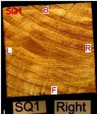
102 Figure 4.20 Sample 1 with square profile (SQ1) 102

103 Figure 4.21 Sample 2 with square profile (SQ2) 103

104 Figure 4.22 Sample 3 with square profile (SQ3) 104

105 4.5 Grain angle determination in 3D space Experiment presented in previous section indicates a clear correlation between measured transmission coefficient magnitude and the arrangement of annual rings, in particular when the cross polarisation transmission is measured. This can be related to the fact that grain usually lies within the plane determined by the annual ring. However, observing the annual ring pattern is not sufficient as grain can be inclined at any angle in the surface determined by a layer. Visual determination of the actual grain angle can be difficult. Observing the set of oven dried samples, it has been noted that some resin leakage occurred along the grain, manifested as darker brown lines on the sample surface. These were used as an indication of the grain direction, as shown in Figure The grain direction was measured on several points within the observed area on all four sides of the sample. The grain angle on the wider side of the sample (marked as front-back direction) was marked as θ and highest measured value is recorded in Table 4.3 as Visually measured θ. The same is done on both narrow sides of the sample (left-right propagation direction) and marked as the Visually measured angle ф in Table 4.3 Figure 4.23 Grain angle determination using a protractor Using the model presented in Section 3.6.2, in particular, Equation (3.38), grain angle values are calculated for first nine samples in Figure Measured transmission coefficient magnitudes, obtained using the measurement setup described in Figure 4.14 and Figure 4.15, are given in Table 4.3, while the following graphs in Figure 4.24 and 4.25 compare visually determined and calculated grain inclinations in these two planes. 105

106 Figure 4.24 Visually and microwave determined grain angles for ten observed samples Table 4-3 Visually and microwave determined grain angles Sample: VV Microwave HH Transmission VH Coefficient VV Magnitude LL db VL Grain angle Visually measured θ Microwave measured Visually measured ф Microwave measured ф

107 Figure 4.25 Correlation between visually and microwave determined grain angles It can be noted that although actual grain angle value is not accurate, the correlation between calculated and measured values is high, as can be noted in both Figure 4.24 and Figure The results demonstrate that the presented technique has a good potential as a practical tool for grain angle determination if additional calibration of the sensor is performed. For this experiment, the free space measurement was not calibrated separately and this error is a contributing factor in observed discrepancies. Currently available calibration procedure for a free space measurement is suitable for nominal polarisation, but not for a cross polarisation measurement. A calibration with standard THRU for free space as total transmission and metal plate as no transmission makes no sense for cross polarisation because both give very similar results (i.e. high attenuation). The calibration procedure for cross polar measurements does not exist and is recommended for future research. 107

108 4.6 Conclusion The theoretical study of the wave propagation through anisotropic media, presented in Chapter 3, shows a relation between the wood permittivity tensor and measured transmission coefficients in nominal and cross polarisation. In this Chapter, this is further investigated in a series of experiments performed using focused beam antenna system. A correlation between grain inclination and the raise in the cross- polar transmission is demonstrated for samples with two-dimensional anisotropy. Then, a problem of threedimensional anisotropy is considered, having in mind a development of a sensor for grain direction determination in lumber. The motivation for this work comes from indications that wood strength and quality in general can be directly related to the grain direction. In literature published to date, the grain inclination is considered only in a plane which is parallel to the wave front of an incident wave [2-9] and it has been described by a single inclination angle θ. Such approach significantly limits practical application of the sensing technique. In this Chapter, the grain direction determination method covers any inclination of grain met in practice, allowing the determination of the grain direction in the tree dimensional space. The definition of the transmission coefficient is extended to show the relationship between the transmitted and incident fields in all four polarization combinations for two orthogonal linearly polarized waves, expressing it in the form of transmission coefficient matrix. It was then demonstrated that both the permittivity matrix and the transmission coefficient matrix become diagonal under the same condition, i.e. when the polarization of an incident field is aligned with a principal direction of the anisotropic media. Thus, in practice, the grain direction measurement does not require the knowledge of the actual permittivity value. It suffices to determine the angles at which the ellipsoid of constant energy is inclined in reference to the coordinate system defined by the three orthogonal polarisation planes, which can be retrieved from the transmission coefficient matrix. The advantage offered by this approach is that we deal with parameters which are easily measured with standard microwave test equipment. Furthermore, only magnitudes of transmission coefficients are needed, which significantly simplifies the problem, because a practical implementation of a sensor measuring magnitude of the transmitted field, rather than its complex values, is much simpler and more economical. The technique demonstrated here shows promising results. Although the actual grain angle value does not closely match the calculated value, the correlation between two data sets is high, with R 2 = 0.74 for θ and R 2 = 0.91 for ф. This indicates that sensor has a capability to detect the variation in the grain angle and accurate values can be obtained by means of an additional calibration. The measurement uncertainty is influenced by absence of free space calibration as well as possible spurious modes of propagation in the observed complex material. It must be also noted here that this technique benefits from broadband operation, as the frequency averaging and smoothing reduces the measurement uncertainty. A more suitable option of calibration standards for free space calibration of cross polar transmission is needed and a future research is recommended. 108

109 5 Heterogeneity analysis: Defect detection and sample categories Introduction The study of a plane wave transmission through wood, presented in this chapter, is concerned with the variation in the sample structure. The focused beam system was used for measurement of twenty two Pinus Radiata samples, presented in Chapter 2. In order to observe the variation of density only, samples are tested in the oven dry condition, i.e. moisture content is zero. Complex transmission coefficient measured at several positions along each sample was used for mapping the density variation along the sample. The free space calibration is performed, as described in section and, in more detail, in section 2.2, and data are stored in three forms, as calibrated (including both PNA and free space calibration), not calibrated (PNA calibration, but no free space calibration) and response calibrated (PNA calibration and response free space calibration). In addition to observation of slow variation in density distribution, the study includes detection of common defects, such as knots, resin pockets and needle flecks. Transmission coefficient distribution is compared with sample properties obtained using CT scans and visual inspection. Data analysis section investigates sample categorisation and its potential use for defect detection and simplified empirical modelling. 5.2 Microwave heterogeneity measurement The experimental study considering sample heterogeneity was performed using a measurement setup presented in Figure 5.1. The aim of this experiment was to investigate detection of the variation in sample structure, in particular, the presence of knots and other internal defects. The sample was moved between the receiving and transmitting antennas, keeping both antennas stationary, and all four S parameters were measured. The size of the sample allowed measurement of twenty points in axial direction, with two successive measurements being one centimetre apart. The use of focused beam antennas minimizes the effect of diffraction from the sample edges. However, the literature on focused beam systems [116] indicates that diffraction effects are avoided only for the case when the minimum transverse dimension of the sample is greater than three times the beam-width of the antenna at the focus. So, with the beam-width being 6 cm, at least 18 cm width of the sample is needed to avoid the diffraction effects. As this is not fulfilled here, the diffraction from the sample edges cannot be avoided. This issue can be approached in several ways. One option is to simply carry on with the measurements, including diffraction effects in measurement uncertainty. Alternatively, we may position the sample between two other wooden blocks, effectively extending the wood surface through which the beam passes and creating matching boundaries. This is approach taken in [39]. Another choice is to position the sample between two absorbers which reduce diffraction effects ( absorbing boundaries ). This is the solution we have adopted in this experiment. The

110 details of measurement setup, showing the absorbers on top and bottom of the sample, are presented in the photo in Figure 5.3. Figure 5.1 The measurement setup for heterogeneity study Figure 5.2 Position of lens, beam and the sample in the experiment 110

111 Figure 5.3 Position of the sample for reduction of diffraction from the sample edges It is noted that diffraction also influences the measurements made close to the edge of the sample (starting and ending edge). As our goal is to observe the variation in density and its effects on the microwave signal, it is best to simply disregard these points and and make conclusions based on the measurements in which only transmitted plane wave are included. In the original measurement setup, we have measured twenty positions along the sample, starting from the beam positioned 9 cm from the edge of the sample. That way, the sample covers the whole aperture of the lens at all times during the measurement and there is approximately one beamwidth length left out (not measured) on each end of the sample (Figure 5.2). Figure 5.4 Distribution of the transmission coefficient magnitudes along the Sample 1 (markers at 4, 7, 15 and 18 cm along the sample show the position at which the measurement should start/stop in order to avoid the effects of diffraction from the edge of the sample) 111

112 Figure 5.5 The schematic of adopted measurement range. To find the acceptable range, a graph of transmission coefficient magnitude is analysed and presented on Figure 5.4. A significant influence of the diffraction from sample edges is noted, showing a typical pattern where the curve first has a steep rise and then goes slightly over the actual value before returning to a value where diffraction has little or no effect. This graph indicates that we ought to disregard additional 7 cm at the beginning and 5 cm at the end of the sample. However, it can be noted that only the steep part introduces a significant error, while overshooting part has a little influence (0.025 db error for the graph in Figure 5.4), which is small compared to the variation caused by defect or a density change. Thus only the points in the sloping part of the graph are disregarded, i.e. first 4 cm and last 2 cm on the sample, leaving us with 15 measured points as indicated in Figure 5.5. Such measurement setup also satisfies a condition set by Ghodgaonkar et al.[116]. In conclusion, only data between points 4 to 18 are taken into consideration in the following analysis. These points are marked on sample photos in Appendix A, showing which part of the sample was scanned and thus indicating which sample features are inside of the observed range Data handling procedure The following data handling procedure applies to each of the four measured polarisation combinations of receiving and transmitting antenna. Data was measured using Vector Network Analyzer and recorded in a standard Touchstone format with the s2p extension. Each file contains [201 x 9] matrix of data. The 201 rows of the matrix present measured frequency points from 8 to 12GHz frequency range, while the measured microwave parameters are organized in nine columns. The first column is the frequency in Hz, followed by Real and Imaginary part of scattering parameters in the following order: S 11, S 21, S 12 and S 22. Figure 5.6 shows a schematic of data structure for one sample, indicating that 20 beam positions along the sample are measured and each measurement is stored in a separate file, resulting in twenty files with a 201 x 9 matrix of data. There are 22 samples in this experiment and schematic of data manipulation is given in Figure 5.7. The data files are processed in Matlab, in order to express them in a format more suitable for data analysis. 112

113 Figure 5.6 Data structure for one sample: 20 files, each containing a full S-matrix for one position along the sample In the format given above, each file contains one position of the beam on the sample, but of interest is a distribution of a single transmission parameter along the sample. Thus we approach each of 20 position files and read one S parameter value, either magnitude or phase, creating thus 8 files for each sample: S 11 magnitude, S 11 phase, S 21 magnitude, S 21 phase, S 12 magnitude, S 12 phase, S 22 magnitude and S 22 phase. Each of these files contains all positions along the sample (matrix size 201x20), as indicated on the flow graph in Figure 5.7. As we are interested in transmission, we analyze the behaviour of S 21 magnitude and S 21 phase. This is repeated for all four polarisation combinations of receiving and transmitting antenna: nominal polarisations VV and HH, as well as the cross-polar measurements HV and VH. Magnitude and phase of Reflection coefficients S 11 and S 22 was measured and briefly analysed, but the dry wood samples show little effect, thus there are no significant findings to report. Figure 5.7 Set of files for 22 samples 113

114 To produce a single graph for each sample, we observe either transmission at single frequency or frequency averaged data. The frequency averaged magnitude is calculated as N 1 1 A av magnitude ( n ) 5-1 N n 0 where magnitude(n) is the measured field magnitude at frequency point n, and N is the total number of frequency sampling points. The average phase is calculated using: 1 N 1 av phase(n N ) n 0 where phase(n) is the measured phase. An un-wrapped phase value is used, obtained by indexing through the phase sample points starting at point n=0, and at each point adding an offset of (r x 360º), where r is chosen to reduce the difference between the current and previous phase values. The averaging over the frequency range is performed not only to reduce the number of data but investigate potential advantage of broadband measurement. Thus we observe and compare frequency averaged data and data at single frequency. As discussed in section 2.2, considering free space calibration, all data are observed in their calibrated, not calibrated and reference calibrated form. From the obtained files, data statistics are calculated: minimum, maximum, range, mean, median, mode and standard deviation for transmission coefficient given by frequency averaged graphs. Finally, each of these graphs is averaged over the whole length of the sample (averaged over all positions) to get a single, bulk value for each sample and we perform a regression analysis, correlating obtained values with bulk moisture or density of each sample. The details of presented procedure will be clarified using examples presented in the following section Density distribution and defect detection The main research question of the heterogeneity study is detection of wood structural features by means of microwave focused beam system. In one aspect of this study, we aim to identify distinctive variations in wood structure, which can be described as detection of defects: knots, remains of branch, needle flecks, resin pockets and change in grain direction. In other aspect, we are looking for slow varying density and moisture distribution along a sample. To study the variation in sample structure, we first group the samples in categories, each having the same type of variation in the structure. Then, we examine how well this grouping correlates with variations noted in measured microwave transmitted field. The variations are related to sample density, as no moisture was present in the samples, i.e. microwave transmission measurements are performed on samples in oven dry condition. 114

115 The following steps are performed: Categories of wood structure which are likely to produce scattering and change in microwave signal are identified by visual and/or X-ray inspection Samples are categorized based on the changes in microwave signal scattering Correlation between microwave signal variation and variation in wood structure, described by the wood category is investigated. By identifying categories of wood structure that are likely to produce change in microwave signal, we can group samples into several categories, which not only serve as a wood grading tool, but may allow easier modelling of wood behaviour within each category Grouping the samples and defect detection We start by identifying which properties of wood structure are more likely to produce change in microwave signal and we define five categories of sample: Samples with large knots Samples with small defects: needle flecks and bright (dense) spots in CT scan Samples with some anomalies Samples with defects outside of the observed zone Clear samples Then, using visual and/or X-ray inspection, samples are sorted, as given in Table 5.1. Table 5-1 Sorting samples into categories Category Category description Samples in this category Colour code used 1 Large defects (knots) 2, 4, 8, 9, 11, 12, 19 Red 2 Small defects (needle flecks, smaller spots) 3, 10, 16, 17, 18, 20, 22 Blue 3 Anomalies 5, 21 Purple 4 Defects outside of the observation zone 7, 14 Yellow 5 Clear wood 1, 6, 13, 15 Green In order to investigate the correlation between the changes in the transmission coefficient and variations in wood structure, we observe changes in the transmitted microwave signal as the beam moves along the sample. The properties of the transmission coefficient magnitude are investigated first, while the phase is considered in the following section. Four polarisation combinations of receiving and transmitting antennas are considered, two for nominal polarization - both antennas vertical (VV) or both horizontal (HH) - and two for cross polarisations. The systematic error in free space measurement system was removed from measured transmission through samples, using TRL calibration procedure, implemented in Matlab, as described in section 2.2. The distribution along the samples is observed for the positions 4 to 18 along the sample, to avoid the diffraction from the sample edge. The value of the transmission coefficient magnitude for each point on the sample is obtained by averaging 201 measured frequency values over the 8 to 12.4 GHz frequency band. 115

116 The resulting transmission magnitude distribution along the sample shows much larger variation in values for samples with knots then for clean samples: a typical dip in the graph occurs when the wave is passing through a knot. The properties of the transmission magnitude characteristics along the sample are described using the statistics of the data, presented in Table 5.2 and Table 5.3, for VV and HH polarisation, respectively. The variation in magnitude along one sample is described using variable Range, which is obtained as a difference between minimum and maximum transmission coefficient magnitude along the measured length of the sample. These three values are given in the first three columns of Table 5.2 and Table 5.3. Another similar indicator, describing the variability in the magnitude values, is Standard Deviation, given in the last column of the tables. The average level of the received signal is described by the Mean value, and mode and median are also enclosed. The data for the Range and Standard Deviation are sorted in descending order and presented in the bar graphs in Figure 5.8 and Figure 5.9, for VV and HH polarization, respectively. The colour code, introduced in Table 5.1, is used to show the sample categories. Observing the measured values presented in these bar graphs, a clear grouping of samples with similar features can be noted. The highest range of magnitude values measured along the sample is obtained for samples with large defects, depicted by red coloured bars. Samples 4, 12 and 2 have particularly high Range and Standard deviation values. The results in VV polarisation have slightly better agreement with visually determined categories (i.e. colour codes) than the data obtained in the HH polarisation, for both high defect (red) and clear (green) samples. The same analysis is done for the Range measured in both cross polarisations and the results are presented in Figure The obtained data show that cross polar transmission magnitude is not suitable for sample categorisation. Further details are given in the following sections, for each category separately. 116

117 Table 5-2 Statistics for VV polarization of calibrated transmission coefficient at 15 points, frequency averaged sample max min range mean mode median st dev Table 5-3 Statistics for HH polarization of calibrated transmission coefficient at 15 points, frequency averaged sample max min range mean mode median st dev

118 Figure 5.8 Transmission coefficient statistics: VV polarization range and standard deviation 118

119 Figure 5.9 Transmission coefficient statistics: HH polarization range and standard deviation 119

120 Figure 5.10 Transmission coefficient statistics: Cross polar magnitude range 120

121 5.3.2 Sample categories and transmission coefficient magnitude Samples with large defects In this category, seven samples with knots are considered. The knot size ranges from 2 to5 cm. The position and orientation of knots within each of the observed samples is different. The sample description and photos are given Table 5.4 and Figure As demonstrated by Heikkila et al. [77], a wave transmitted through a wood sample has much higher attenuation when passing through knots then through the unblemished part of the sample. This is confirmed in Figure 5.12, which shows transmission coefficient magnitude measured for the seven samples. Comparing graphs with sample images given in Figure 5.11, we note that lower transmission magnitude coincides with the position of the knot on the sample. Using the variation in transmission coefficient magnitude as an indicator of the presence of knots, we calculate the Range of magnitude values, as described in the previous section, and use it to identify the sample categories. The graphs from Figure 5.8 and Figure 5.9 are replicated in Figures 5.13 and 5.14, respectively, now clearly showing the samples within observed category with large defect. It can be seen that samples with knots (given in red colour and marked with arrows) have higher Range in both vertical and horizontal nominal polarisation (VV and HH), then it is the case for the clear samples or the ones with minor defects. Two graphs showing the Range of transmission coefficient magnitudes for two cross polarisations (VH and HV) are also enclosed, in Figure The cross polar magnitude is expected to have high Range when the grain angle changes along the sample. Bar chart shows that, even though this is the case for some of the samples, it is not a general rule, and the grain angle recovery may appear further along the sample after a major defect in wood structure. Table 5-4 Description of samples in category 1 Samples with large defects (category 1, colour code red) Sample A big knot, at the lower end of the sample, goes all the way through and is visible at the base. CT reveals additional smaller defects inside: a cm or so before the knot there is a needle fleck defect. The effect of the knot is visible along 7cm length of the sample. It is expected that the knot affects the second part of 2 the microwave transmission graph. Branch remains on front, in the first part of the sample and noticeable as a grain disturbance at the back of the sample. The branch doesn t go all the way into the sample, so on the top it is noted only as a cm wide 4 blemish. In microwave scan, we expect reaction to the knot at the start of the graph At the very start, this sample is clear, followed by some needle flecks in the first part of the observed sample length. In the second part, there is a big knot, going from the middle of the front side down to the 8 base of the sample (not visible on the back or top). Knot and pins: Knot is in approximately in the middle of the observed area. This knot does not look very bright in CT scan (not very dense ) and it occupies just about a quarter of the sample cross section. 9 However, more defects (two needle flecks) are found in the second part of the sample. A small knot at the very beginning of the scanned area, it is positioned at the lower third of the sample, 11 going from front to the base. Otherwise, the rest of the sample is clear. Because of the error in CT positioning, this knot is not visible on ct scan, but it is clear in the photo and at the very beginning of the microwave scan. The knot is not large but goes all the way through the sample 12 and it is positioned almost perpendicular to the annual rings 19 has a knot at the end of scanned area. 121

122 Figure 5.11 Samples from category 1 122

123 Figure 5.12 Measured transmission coefficients for Category 1 samples (VV and HH polarisation) 123

124 Figure 5.13 Statistics for VV polarisation of samples in category 1, as indicated by the arrows 124

125 Figure 5.14 Statistics for HH polarisation of samples in category 1 125

126 Figure 5.15 Statistics for cross polarisation of samples in category 1 126

127 Presented graphs show that transmitted microwaves react significantly to the presence of knots, regardless of their position within the beam. Biggest Range is noted for Sample 12, which has a knot passing all the way through the sample, as if a branch is going all the way through starting from the top corner and going almost down towards the middle of the sample. The knots are detected on sample edges (as in Sample 4) as well as in the middle of the sample, as in Sample 9. The smallest Range is detected for Sample 11, which has a 2cm knot occupying a lower third of the sample. There are several theories to the cause of this reaction. We can speculate that, for the oven dry wood, the permittivity value and thus the attenuation through the wood is most strongly influenced by the density of the wood matter. However, we have confirmed in Chapter 2 that knots are not necessarily denser than the surrounding wood matter. If we assume that variation in the microwave signal is caused by the change in the material density, then we can expect higher attenuation from knots which have higher density. This is true for Sample 9, where a knot having a lower density, as indicated by CT scan, shows lower attenuation of transmitted signal then its more dense counterparts. However, this is not true for Sample 4, which shows much higher attenuation then Sample 8, yet the density of its knot, indicated by the gray scale of CT scan, is not nearly as high as in the case of Sample 8 (Figure 5.16). Sample 4 Sample 8 Figure 5.16 CT scan of samples with knots: Sample 4 (left) and Sample 8 (right) Alternative explanation is offered by Heikkila et al. [77], who suggest that a plane wave travelling through wood generates a hybrid HE 11 mode in a knot, which he models as a dielectric waveguide. This theory cannot be confirmed here, as the biggest change in transmission coefficient magnitude is caused by the sample whose knot goes almost vertically from the top to its base and it is hard to imagine how an HE 11 wave mode is excited in this knot. We speculate that possible answer for the high attenuation in knots lies in the wood structure, not only in the knot, but in the surrounding wood cells, supporting the wood growth around the knot Samples with small defects In this category, some damage on the sample exists, although not as significant as in the case of samples with knots. Some of the samples have knots at the edge of the observed area, such as Samples 3, 10 and 20. Other samples in this category have some minor defects, such as a needle fleck or a hidden branch. For example, Sample 18 does not have any knots, but has needle flecks visible on several CT scans, while for Sample 17 that damage is much wider and looks like a hidden branch. Measured variations of transmission magnitude along the sample are presented in Figure 5.18 where graph legend indicates the polarisation of the receiving and transmitting antenna (letters VV or HH), while letter m, which for stands for magnitude, is followed by the number of the sample (i.e. 3, 10, 16, 17, 18, 20 and 22). Thus the magnitude of sample 3 127

128 measured in VV polarisation is labelled as VVm3. Figure 5.19 shows that, for majority of samples in this category, VV Range is almost double of the value obtained for the clear samples (i.e. 3,10, 16,17). The remaining samples from this group (18, 20, 22) have, on average 50% higher VV Range than the samples from clear category. Similarly, for HH polarisation, the Range is, on average, 50% higher for samples with mild defects then for the clear samples. The graphs for Range of transmission coefficient magnitudes for two cross polarisations (VH and HV) are enclosed in Figure Again, it can be assumed that grain direction changes around a defect, causing depolarisation and thus a change in the cross polar level. The bar charts in Figure 5.21 show that, even though this is the case for more than half of the observed samples (i.e. samples 3, 10, 18, 20), some samples were not affected by it (samples 16, 17, 22). Figure 5.17 Samples in category 2 128

129 Table 5-5 Description of samples in category 2 Samples with small defects (category 2, colour code blue) Front, back and base are unblemished, but the top side has a knot at the very edge of the sample; this knot is outside of the measured zone, but CT scan reveals several needle fleck 3 defects. A big knot on this sample is slightly outside the measured zone, but more defects are revealed 10 by CT scan: some needle flecks in the second half of the scan 16 No visible surface damage, but CT reveals a defect. 17 No visible surface damage, CT reveals a defect. 18 No visible surface damage, some needle flecks are detected on four CT slides A knot at the end of the sample, slightly outside of the scanned area. Some needle flecks are 20 noted. 22 No visible surface damage, but few bright spots, indicating defects, revealed by CT scan sample Figure 5.18 Transmission coefficient distribution for samples in category 2 129

130 Figure 5.19 Statistics for VV polarisation of samples in category 2 130

131 Figure 5.20 Statistics for HH polarisation of samples in category 2 131

132 Figure 5.21 Statistics for cross polarisations of samples in category 2 132

133 Samples with noted anomalies in structure Samples in this category have shown some peculiar behaviour, thus are sorted in a separate category. Sample 5 looks clear and on the surface has very little damage (a couple of needle flecks, but very clear otherwise). To gain more insight in sample properties, this sample was measured in oven dry condition and with 11% moisture content (the data at 11% moisture content was available from the study presented in Chapter 6.)Figure 5.22 shows the range of Sample 5 compared with other samples, for 11% moisture content. It shows that Sample 5 has a very high range in HH polarisation, and relatively high range in VV polarisation. That was not expected from a sample with no visible defects. However, after the oven drying (reducing moisture content to zero), the Sample 5 shows very small Range in both polarisations, in particular in HH polarisation, presented in Figure CT scan reveals a crack in the sample, and it is reasonable to assume that this crack was a resin pocket. As for Sample 21, comparison of the left and the right end of the sample shows that the annual rings are not matching. This indicates a change in ring orientation along the sample. Table 5.6 and photos in Figure 5.23 describe the samples, while graphs in Figures 5.24 to 5.27 show the behaviour of these samples. Figure 5.22 Statistics for sample 5 measured at 11% moisture content Figure 5.23 Samples in category 3 133

134 Table 5-6 Description of samples in category 3 Sample Samples with noted anomalies in structure (category 3, colour code purple) 5 Looks clear on the outside. After drying has an interior crack visible on the CT scan. 21 Has a change in annual ring orientation along the sample Figure 5.24 Transmission coefficient distribution for samples in category 3 134

135 Figure 5.25 Statistics for VV polarisation of samples in category 3 135

136 Figure 5.26 Statistics for HH polarisation of samples in category 3 136

137 Figure 5.27 Statistics for cross polarisations of samples in category 3 137

138 Samples with defects outside the observed volume The samples in this category are effectively clear, as there are no defects inside of the observed range. However, as a defect exists outside observed zone, they are separated in own category. Table 5.7 gives a list and description of the samples in this category, while their appearance is shown in Figure The magnitude of measured transmission coefficient, presented in Figure 5.29, shows very little variation when measured along the sample. This is also visible by a small range and standard deviation values for both VV and HH polarisation, presented in Figures 5.30 and 5.31, respectively. The presented results show that samples in this category behave as clear samples. This, in addition, demonstrates the ability of applied sensor to focus its beam on the observed area of sample, proving that defects outside the observed volume have little influence on measured transmission. The cross polar transmission magnitude, whose range of variations along the sample for VH and HV polarisation is presented in Figure 5.32, indicates that both samples have their grains aligned with a principal direction. Table 5-7 Description of samples in category 4 Samples with defects outside observed volume (category 4, colour code yellow) sample 7 The defect (very small knot) is outside of measured area, in measured region the sample is clear 14 Has knot outside of the scan range, small defect on ct scan: two or three very pale rays Figure 5.28 Samples in category 4 138

139 Figure 5.29 Transmission coefficient distribution for samples in category 4 139

140 Figure 5.30 Statistics for VV polarisations of samples in category 4 140

141 Figure 5.31 Statistics for HH polarisations of samples in category 4 141

142 Figure 5.32 Statistics for cross polarisations of samples in category 4 142

143 Clear samples Clear samples have no distinctive blemishes and defects. It is typical for the Pinus Radiata species, to have a grouping of branches around the trunk at certain height of the tree and areas between them with no branching, known as whorls and internodes. It can be assumed that samples considered here are from this, clear, part of the log. The list of these samples is given in Table 5.8 and Figure 5.33 presents the images of the clear samples. Table 5-8 Description of samples in category 5 Clear samples (category 5, colour code green) Sample 1 Clear 6 Clear 13 Clear 15 Clear (small grain defect at the very end of sample) Figure 5.33 Enhanced images of clear samples, belonging to category Figure 5.34 shows measured transmission coefficient distribution along the sample. There is very little variation in the magnitude of transmission coefficient, as it was expected. This is described in more details in Figure 5.35, where transmission variation is depicted for each sample separately, using finer scale for Transmission magnitude values. It can be seen that the variation of magnitude does not exceed 1.5 db for VV polarisation. This can be further seen on graph in Figure 5.36, where Range and Standard deviation for VV calibration are presented. Figure 5.37 shows these parameters for HH polarisation, where, again, there is very little variation in signal magnitude for all clear samples. Figure 3.38 shows the cross polar Range for both HV and VH polarisation and indicates that some grain inclination is present in all four observed samples, though not significant, i.e. Range is around or less than 5 db. 143

144 Figure 5.34 Transmission coefficient distribution for samples in category 5 144

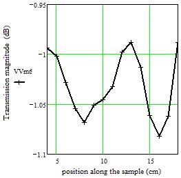
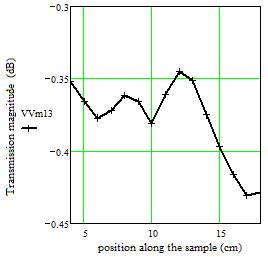
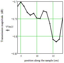
145 Figure 5.35 Details of transmission coefficient distribution for samples in category 5 145

146 Figure 5.36 Statistics for VV polarisation of samples in category 5 146

147 Figure 5.37 Statistics for HH polarisation of samples in category 5 147

148 Figure 5.38 Statistics for cross polarisations of samples in category 5 148

149 5.3.3 Transmission coefficient phase measurement Transmission coefficient, measured as a ratio of the field transmitted through the wood sample and the field incident to the sample front surface, is a complex value and besides its magnitude, whose properties are considered above, has a phase value. In the following set of graphs, in Figure 5.39, the properties of the transmission coefficient phase is considered, measured in two nominal polarisations of transmitting and receiving antennas. Again, when both antennas are horizontally polarised, the polarisation is marked as HH, while VV indicates that both antennas are in vertical polarization. The data presented here are from the frequency averaged transmission coefficient value and TRL calibration is used for the removal of the measurement systematic error of the free space transmission measurement system. In this section we consider the sample categories based on the defects and sharp variations in the sample structure, as adopted above. To show the relationship between the phase and the variation in wood density along the sample, we observe the change in phase values along the sample, considering it as an indicator of a defect presence in the sample. It is hypothesised that a large range of phase values along the sample indicates the presence of defects as well as variation in sample density. The absolute phase value of is of no interest, only the range of phase variations along the sample. However, it has been noted that the mean of measured phase values for each sample differs significantly, which makes it hard to compare them by plotting the graphs together, as the resolution of such plots is not sufficient for detection of subtle variations in signal level. In other words, the variation of phase along the sample is often smaller than 0.1 degrees and if the graphs are presented on (-180, 180) range, to accommodate for the variation in mean (absolute) levels from one sample to the other, there is not enough resolution to observe 0.1 deg variations. For that reason, the mean value of each phase graph is adjusted so that all samples have approximately the same mean level. This allows us to compare the range of variations in the phase distribution along the sample. Samples 2, 4, 8 and 12, have large knots and have demonstrated high range in magnitude values, are also showing the high range in phase values, in both HH and VV polarisation. However, other samples do not show such a clear category grouping as it was the case with the magnitude range measurement. We hypothesize here that the phase reacts more to the actual sample density and because some of the defects have no significant variation in density (as demonstrated in Chapter 2, showing knot detection using CT scans), these are not distinguished in the phase graph as significant obstacles. The detail consideration of this claim is presented in the following Chapter, considering detection of slow variation of density along the wood sample. 149

150 Figure 5.39 Phase variation (deg) along the sample for HH and VV polarisation, grouped by categories 150

151 Figure 5.39 Phase variation (deg) along the sample for HH and VV polarisation, grouped by categories (cont.) 151

152 Figure 5.39 Phase variation (deg) along the sample for HH and VV polarisation, grouped by categories (cont.) 152

153 Figure 5.39 Phase variation (deg) along the sample for HH and VV polarisation, grouped by categories (cont.) 153

154 Figure 5.40 Range of transmission coefficient phase 154

155 5.4 Conclusion The lumber heterogeneity mapping using a microwave focused beam transmission measurement has not been previously reported, although this sensor was used before for bulk moisture content and density measurement. The first part of heterogeneity study, presented in this Chapter, is concerned with detection of wood structural features by means of microwave focused beam system. The aim is to identify distinctive variations in wood structure: knots, remains of branch, needle flecks, resin pockets and change in grain direction. This can be described as detection of defects, as most of these features affect structural integrity of lumber and should not be present in a high quality lumber. This is an additional novel aspect, as defect detection studies conducted so far were commonly performed for knot detection, but here was extended to include microwave signal variations due to needle flecks, cracks, resin pockets and annual ring variations. The beam size was comparable to the width of the sample thus the whole volume of the sample was inspected. This is demonstrated on samples where knots were positioned at the very edge, but still got detected. A disadvantage the Gaussian beam which is wide in comparison to the sample width is diffraction from the sample edges. This was remedied by surrounding the sample with absorbing material. However, the practicality of this approach in industry is yet to be estimated. The large amount of data was collected measuring 20 positions on each of 22 samples for four polarisation combinations (VV, VH, HV, HH). All four complex S parameters are measured, at 201 frequency points over the 8 to 12.4 GHz frequency range. The data handling procedure is briefly described, as well as the process of calculation of signal parameters used for defect detection and sample classification. Visual inspection and CT scan of the samples were used to establish five categories of samples, based on the presence of defects. The transmission magnitude was averaged over the measured frequency range and some basic statistics of the data along the sample was calculated. The measured data demonstrate that the range of transmission magnitude values over the sample length, as well as the standard deviation, can be good indicators of the presence of defects within the observed sample length. The mean value of transmission coefficient magnitude calculated for the data obtained over the 16 cm length along the sample is related to sample density. Slow variations of the density along the sample cannot be detected using magnitude, but averaged mean value correlates well with the bulk density of the sample. It was also demonstrated that better empirical models can be used if the data for samples with large defects are omitted. The phase of the transmission coefficient is also considered, but appears less efficient for defect detection than the magnitude. Further analysis of phase properties is given in the following Chapter, considering slow variation of density along the sample. 155

156 6 Heterogeneity analysis: Mapping density and moisture distribution 6.1 Introduction It has been hypothesised that wood structure is not homogeneous and that, besides fast varying changes in the structure, corresponding to knots and defects, there are also some slower varying changes, corresponding to density or moisture variation along the sample. Thus, in this section, the focus is shifted from defect detection to density variation mapping, observing its gradual change along the sample. The study is further extended to include free space calibration and analysis of broadband transmission measurement, exploring its advantages and limitations for industrial application, as introduced in section and section 2.2. In the concluding section of this chapter, a study of moisture and density distribution is considered. Seven Pinus Radiata samples are measured and analysis of total density distribution for four different moisture content levels is performed. A study of simultaneous detection of moisture content and density of the sample is enclosed. 6.2 A slow variation of wood density Observing the variation in transmission coefficient magnitude given in Figure 5.35 for four clear samples, we note that little difference exists between the four graphs. In addition, the change in transmission coefficient magnitude along the sample is very small and it is more likely related to the portion of systematic error that has not been removed by TRL calibration. The phase of the transmission coefficient seems like a better candidate for this study. In addition, there were some reports which state that the phase is more sensitive to changes in sample density than the magnitude of transmitted wave [79]. To investigate the change in density, we first need to establish the actual density variation in the sample. One way is to cut, weigh and measure the samples, but this is not a practical solution. An alternative used here are the readouts from CT scans, which are the density related values. We have measured the variation in density on a clear wood sample using CT scan images on Dycom reader. Again, we are not looking at the absolute density value but for the variations from one slide to another. There was a need for some pre-processing of CT data, before they can be compared to the microwave graphs. First issue was to identify the slides which describe the volume illuminated by the Gaussian beam for each of the measured microwave positions. In this case, a 6cm wide beam illuminates the volume described by thirteen CT slides. The readout data are obtained as a mean value from Dicom reader. These density-related values are then averaged over thirteen slides to obtain a single reference value for each beam position. This was possible to perform for beam positions 8 to 17. The results are presented in the set of graphs given in Figures

157 density variation CT mean readout value phase variation (deg) position along the sample (cm) position along the sample (cm) phase variation (R 2 =0.6681) Figure 6.1 Slow variation of wood density: Sample 1 157

158 Density variation density variation phase variation (deg) position along the sample (cm) position along the sample (cm) Phase variation (R 2 =0.502) Figure 6.2 Slow variation of wood density: Sample 6 158

159 density variation density variation phase variation (deg) position along the sample (cm) position along the sample (cm) phase variation (R 2 =0.9292) Figure 6.3 Slow variation of wood density: Sample 5 159

160 density variation density variation phase variation (deg) position along the sample (cm) position along the sample (cm) phase variation (R 2 =0.842) Figure 6.4 Slow variation of wood density: Sample 7 160

161 These allow comparison of the phase variation along the sample (given in the first graph in each figure) with density variation along the sample (middle graph), for samples 1, 5, 6 and 7. The last graph in each Figure shows calculated correlation between two graphs, with calculated R 2 values ranging from to Observing the first two graphs given in Figures 6.1 and 6.2, showing Sample 1 and Sample 6, respectively, it is clear that negative correlation exist, showing that phase of the transmitted coefficient increases with the decrease in density of the observed sample volume. It can be concluded that a low correlation obtained for Sample 1 and Sample 6 (R 2 of and , respectively) is a consequence of misalignment of two graphs, so that points on the graphs don t relate to the same point on the sample. This has little effect on the sample with constantly increasing density (Sample 5, given in Figure 6.3, with R 2 = ), while small misalignment is noted for Sample 7 (Figure 6.4), with minimum density value occurring at point 7 and the peak on the microwave phase variation graph is at the point 6. Consequently, correlation is slightly poorer then for Sample 5, having R 2 value of The obtained results, thus, show that phase variation can be used as a good indicator of slow variation in sample density. 6.3 Bulk density measurement The study of microwave detection of bulk density was conducted using the data obtained for twenty two samples, measured in two orthogonal nominal polarisations. The mean value of microwave transmission coefficient is calculated from transmission at twenty points measured along the sample. We are looking for correlation between microwave signal and bulk density for each of twenty two samples. In addition, the experimental data confirm that categorizing can improve accuracy in final MC and density determination, as better correlation is achieved when data for samples with large defects (red category) are omitted. For VV polarization, a fairly good correlation between bulk density and mean magnitude is obtained, with R 2 = The results are presented in Figure 6.5. It is significantly improved when samples with knots are omitted and R 2 is 0.837, as Figure 6.6 indicates. Figure 6.5 Bulk density correlation with measured microwave Transmission coefficient magnitude, VV polarisation 161

162 For HH polarization, the relation between Transmission coefficient magnitude and bulk density is given in Figure 6.7. There is no significant change in the correlation when the samples with knots are omitted. Figure 6.6 Bulk density correlation with measured Transmission coefficient magnitude, VV polarisation, clear samples Figure 6.7 Bulk density correlation with measured Transmission coefficient magnitude, HH polarisation, all samples 162

163 Measurement calibration This research considers an importance and feasibility of the free space calibration in an industrial environment, as introduced in section and section 2.2. The benefits of the full TRL calibration and its potential replacement with Response calibration for a practical industrial application are considered. In all Focused Beam measurements conducted in this thesis, two calibrations are performed. First, the Network Analyser is calibrated at its coaxial ports using a built-in full two-port SOLT calibration procedure on the Network Analyzer (Agilent PNA-L) and a set of Agilent calibration standards (Agilent 3.5mm Economy Calibration Kit 85052D). The reference plane was at the end of coaxial cables used to connect horn antennas to the Network Analyzer. Even though the cables are moved and bent after the calibration, in order to reach the antennas in their required positions, little error is expected here as a set of high quality Huber and Suhner Sucoflex cables was used, highly recommended for this type of measurements. The second calibration is then performed, to eliminate the systematic errors from the free space setup. In this work we have opted for TRL calibration. However the calibration was not performed using in-build Network Analyzer calibration procedure, but with a custom made TRL calibration code, implemented in Matlab. For every experiment performed in this thesis, in addition to sample measurement, the measurement of three calibration standards was performed. In this section, we consider the importance of the free space setup calibration, assuming that Network Analyzer calibration (the first calibration) is always performed, both in laboratory and in the industrial environment Comparison of calibrated and not calibrated data The data to which no error correction is applied shows considerable loss which is not exclusively related to the attenuation through the sample. In addition, the data measured over a frequency range shows a ripple pattern, indicating an interference of the measured signal with a frequency dependent error vector. This is demonstrated in Figure 6.8 and Figure 6.9, showing frequency dependent transmission coefficient magnitude (Insertion Loss, db value of S 21 magnitude) for five dry wood samples, measured through the middle of the sample at VV polarisation. The graph in Figure 6.8 shows measured transmission through the sample without free space calibration, while Figure 6.9 shows the same data with applied TRL error correction. Comparing these two graphs, we note that calibrated data show expectedly low attenuation through dry wood samples as well as reduced frequency dependent ripple. The same effect is noted observing the rest of the samples as well as for the same lot of samples measured at 11% moisture content. However, there is still some amount of ripple present on the measured trace, indicating the presence of residual, post-calibration error. There are several reasons for the existence of the residual error, including imperfections in the calibration standards, the instrumentation and the coaxial cables connecting the spot-focusing antennas to the test ports of the S-parameter test set. When working with PNA, the instrumentation errors (e.g., frequency instability, power variation of microwave signals) are negligible. It is commonly accepted that the residual source and load

164 mismatch errors due to imperfections in the calibration standards are responsible for the remaining ripple. Figure 6.8 Transmission magnitude for five dry samples, not calibrated Figure 6.9 Transmission magnitude for five dry samples, calibrated data Dealing with residual errors The ripple noted after the TRL calibration indicates the presence of some residual postcalibration error. This was reported in literature considering TRL calibration, in studies performed using high quality standards [74], [116], [117], [123]. It can be concluded that the residual error cannot be further minimized by perfecting TRL calibration and has to be dealt with separately. There are several solutions, proposed in the literature, for dealing with the post-calibration residual error. Ghodgaonkar et al. [116] recommend time-domain gating, implemented using the gating feature of an Agilent Network Analyzer (HP8510B). Alternatively, this can be done in a 164

165 post processing procedure, assuming that measurements are performed over a sufficiently large number of frequency points. For implementation of time-domain gating, the frequency domain data are first obtained for measured S parameters. Then, taking the inverse Fourier transform, the time domain data are obtained. Then, the gating is applied over the time domain response which includes the main transmission (or reflection) response and multiple reflections from the sample. The Fourier transform of the gated time-domain response gives the frequency-domain response with time-domain gating. Further details are given in [56]. Alternative solution is offered by [123], who used smoothing techniques to minimize the ripple. Time-domain gating is an expensive feature and not all VNAs are equipped with it. In addition, the whole procedure is time consuming and thus not practical in industry. Thus Gagnon et al. propose smoothing as a means of correcting measured S-parameters. The smoothing algorithm was implemented in Mathcad, using a function that was predefined in the software and good results are reported. The smoothing function enables the user to transform measured data by averaging it versus frequency. Percentage smoothing is calculated by the dividing the percentage of frequency span that is averaged (the "aperture") by the total swept bandwidth. In the examples below, Mathcad Plus was used to perform smoothing on four samples using medsmooth(vy,n) function, which returns an m-element vector created by smoothing VV with running medians. Here, VV is the function (an m element vector of real numbers, in our case 201 frequency points at which the microwave transmission is measured) and n is the width of the window over which smoothing occurs. Here, n must be an odd number of elements less than the number of elements in VV. In our case, n = 51, even though the ripple is significantly reduced for n>20. Instead of time domain gating, we have opted for smoothing and frequency averaging as an option to partially remove the effect of error ripple. Minimising error using frequency averaging is not an error removal technique. However, we know that the fast varying ripples existing on the graph are not caused by the material response but by the vector addition of error signal. So, we can use smoothing to reduce the effect of ripples and find the more accurate transmission magnitude value. One of the fastest but admittedly the least accurate ways is to frequency average the measured results. In a more accurate version, we should employ one of the smoothing techniques. Frequency averaging over the whole measured bandwidth, proposed here, is similar to the approach used in [88] and [112]. The frequency-averaged magnitude and phase are calculated as A 1 N 1 av A(n N ) and 1 N 1 n 0 av phase(n N ) n 0 where A(n) is the measured field amplitude and phase(n) is the measured phase at frequency point n, and N is the number of frequency sampling points. This approach was not used so far for combating the residual post-calibration errors and we investigate its suitability, comparing it with smoothing. Figure 6.10 shows measured transmission coefficients for three samples (Sample 1, Sample 2 and Sample 3), measured over the frequency band of 8 to 12.4 GHz. The blue line, marked as Ai, is obtained by smoothing function in MathCad, while red line, marked as Aver shows the transmission coefficient obtained by averaging the values over the frequency range. The 165

166 smoothing function shows little or no residual ripple, while frequency averaging offers a good estimate of the transmission magnitude level. Figure 6.10 Smoothing and frequency averaging 166

167 Figure 6.11 Calibration and defect detection The application of TRL calibration and frequency averaging improves the accuracy in wood property detection. In Figure 6.11, a set of two graphs shows how calibration improves defect detection accuracy. Both bar graphs are obtained by frequency averaging magnitude of transmitted wave and calculating range of values over the 15 points measured along each sample. The top graph shows data for calibrated and the bottom graph for not calibrated data. Improvement in data grouping, indicated by colour codes, can be noted. 167

168 One factor which has a great impact is the operating bandwidth. The measured data indicate that working over the larger number of frequency points is beneficial. The first advantage is offered when dealing with the phase data, as working over a bandwidth of frequencies allows us to unwrap the phase and avoid the ambiguity which occurs due to the phase periodicity, reported in [39] HH transmission, 8GHz, not calibrated, first five samples Series1 Series2 Series3 Series4 Series Figure 6.12 Transmission magnitude for first five samples at 8 GHz, not calibrated values Series1 Series2 Series3 Series4 Series Figure 6.13 Transmission magnitude for first five samples at 8 GHz, calibrated values Further benefits can be noted by observing the following set of graphs given in Figures 6.12 and 6.13, showing the transmission magnitude for the first five samples, measured at twenty points along each sample. Figure 6.12 shows not calibrated data, measured at single frequency. Calibrated data given in Figure 6.13 show that the most significant change is seen in sample 4, which is a sample with a large knot. The variation due to the knot is much more pronounced in calibrated data, allowing for more accurate defect detection. 168

169 The difference between calibrated and not calibrated data is not so pronounced when working with frequency averaged data: graphs in Figure 6.14 and 6.15 show similar amount of range variation HH magnitude, fav, calibrated, first five samples Series1 Series2 Series3 Series4 Series Figure 6.14 Transmission magnitude for first five samples, frequency averaged, calibrated values HH magnitude, fav, not calibrated, first five samples Series1 Series2 Series3 Series4 Series Figure 6.15 Transmission magnitude for first five samples, frequency averaged, not calibrated values 169

170 Advantage of working over a bandwidth when dealing with defect detection is further presented in Figure 6.16 and 6.17, which show the range of data for 22 samples, grouped in five defect categories and colour coded. Both of these graphs show calibrated measurements. It can be seen that residual ripple remaining in single frequency graph causes a less pronounced difference between samples with knots, in particular samples 2 and 8, when compared to the sample with mild defects. In addition, samples without defects, 6 and 13, have the range similar to the samples with defects (blue category). The frequency averaged values have bigger difference between clear samples (green and yellow category) and samples with defects (blue and red categories). Figure 6.16 Bandwidth and defect detection: single frequency Figure 6.17 Bandwidth and defect detection: averaged over frequency band 170

171 6.4.2 Response calibration In addition to the vector calibration methods presented above, there is a simple but less accurate way to correct systematic error terms called Response calibration. The Response calibration is simple to perform, but corrects for only a few of the twelve possible systematic error terms (namely, reflection and transmission tracking). This is a normalized measurement in which a reference trace (usually free space transmission) is stored in memory and the stored trace is divided into measurement data for normalization. Separating free space calibration procedure was useful, as it provide us with the opportunity to study the benefits of the TRL and Response calibration in wood measurements. This approach allows us to compare the performance of the system when calibration is omitted, when only a response calibration is performed and when the full TRL calibration is applied. To see if it is sufficient to perform calibration using Reference calibration procedure only, we compare the ripple from calibrated and ripple from reference calibrated graph, given in Figure 6.18 and note that very little improvement is made in the ripple reduction, when broadband data is considered. We may argue that standards used in this experiment were by no means of particularly high quality and there is plenty of space for improvement of their execution. On the other hand, the execution at hands allows us to estimate a robustness of the procedure, which is essential for the industrial environment. One can argue that if such robust set of standards cannot bring the improvement when compared to response calibration or complete omission of free space calibration, then calibration step may be considered for laboratory environment only. Alternatively, another calibration procedure could have been chosen and potentially offer better results. For example, in TRM procedure there is no need for movement of the antennas, thus reducing the error due to cable bending and antenna repositioning. In addition, avoided is a potential error due to Line standard calibrated over the frequency range, as it is known that movement of the antenna for the quarter wavelength length applies to the central frequency only. However, the TRM procedure requires a good quality match standard which could be hard to maintain in the industrial environment and which many not be an economical solution. 2 0 Transmission magnitude vs frequency, Sample 1, dry calibrated not calibrated free space response calibrated Figure 6.18 Comparison of calibrated, not calibrated and response calibrated transmission magnitude 171

172 6.5 Dry density and total density distribution Polarisation dependent response Microwave signal variation was observed for a group of 21 samples with MC11% and again when these samples are oven dried. When comparing transmission through a set of samples in these two conditions, it is noted that much bigger difference in signal level occurs in HH polarization then in VV polarization. This is demonstrated in Figure 6.19, using Sample 12 as an example. Two enclosed graphs show transmission through dry and MC11% sample for VV and HH polarization, respectively. It can be noted that the difference in signal level of is approximately 5dB for VV polarization, but almost 8dB for HH polarization. Figure 6.19 Comparison of transmission through dry and 11% MC sample in VV (top) and HH(below) polarisation The transmission coefficient magnitudes for remaining samples are presented in Table 6.1. This Table includes not only measured VV and HH transmission coefficient magnitudes for 11% MC (given as VV and HH in Table 6.1) and dry wood values (given as dvv and dhh ), but also a manipulation of these data, in form of difference between these values. For VV polarization, difference between dry and 11% MC values is given as dvv-vv, while for HH polarization the corresponding parameter is given as dhh-hh. Difference between the values 172

173 related to two polarisation and same moisture content is also given for dry condition (dvv-dhh) and 11% MC condition (VV-HH). These last two parameters are presented in Figure 6.20, showing that significantly larger difference between responses for moist wood than for the dry wood. A possible explanation is that the way the water is binding to cellulose greatly contributes to the sample anisotropy. This can, therefore, be used as an indicator of change in moisture content of the sample and used as a means to distinguish between MC and density contribution. Table 6-1 Density and moisture density relation to polarisation of transmitted wave Sample VV Dry VV dvv - Dry HH dhh - dvv - HH (dvv) VV (dhh) HH dhh VV-HH (no knot) with knot no knot with knot Figure 6.20 Illustration of difference between dry and 11%MC magnitude level for HH and VV polarisation 173

174 6.5.2 Variation of density and moisture density A set of seven new samples, with densities 342, 349, 409, 436, 449, 460, 459 kg/m 3, are measured at four moisture content levels: dry (0.2%), 6%, 8% and 15%. The width of these samples allows the measurements without absorbers around the samples. Figure 6.21 Variation in density and moisture content in HH (top) and VV (below) polarisation 174

175 HH transm magnitude, S1 The magnitudes of two nominal polarisations are presented in Figure As in the previous experiment, it can be noted that HH polarisation is much more affected with the change in moisture content than the VV polarisation. Transmission magnitudes are given in Tables 6.2 and 6.3. The tables also contain calculated regression coefficients, showing that the change in microwave transmission magnitude correlates well with the change in moisture content for both HH and VV polarisation, having R 2 ranging from and , respectively. The correlation with density is lower for the transmission magnitude, with better correlation obtained for more samples with higher moisture content. A selected data are presented in Figure 6.22 and Figure 6.23, as an additional illustration of presented values. Figure 6.22 shows the correlation between MC and microwave transmission magnitude for sample 1, four MC levels, indicating good correlation between two values. Figure 6.23 illustrates the correlation between dry density and microwave HH transmission magnitude for 15% MC value. The correlation is 0.92, as shown in Table 6.2. Table 6-2 Transmission magnitude for HH polarization HH Mag(dB) MC % (Actual MC) 0 % 6% 8% 15% Correlation Sample Dry Density (0.2) (6. 5) (8) (15.4) with MC Correlation with density Moisture content Figure 6.22 Correlation between MC and microwave transmission magnitude for sample 1, four MC levels 175

176 HH transmission, 7 samples, MC15% Dry density Figure 6.23 Correlation between dry density and microwave HH transmission magnitude: MC =15% Table 6.3 shows the correlation with moisture content and correlation with density for VV polarisation, while the graphs in Figure 6.24 and 6.25 depict the correlation between dry density and moisture content, respectively. Good correlation is noted for moisture content, as the coefficients presented in Table 6.3 indicate, while poor correlation was obtained for density data. The HH polarisation has better correlation with bulk density then VV polarisation, which confirms the findings in Section 6.3. However, the correlation coefficient for VV polarisation obtained here are very low. Much better correlation with density is obtained when polarisation of the receiving and transmitting antennas are inclined 45 relative to the sample axis (to the VV direction). If the inclination is 45 counter clockwise from vertical axis, the polarisation is called LL, while 45 clockwise inclination forms RR polarisation. The data obtained for magnitude of RR and LL polarisation are presented in Tables 6.4 and 6.5, respectively. The results for RR polarisation data are presented in Table 6.4 and illustrative graphs given in Figure Both graphs, for moisture content (top) and for density (bottom), show good correlation with measured microwave transmission coefficient magnitude. Similar results are obtained for LL polarisation, as seen in Table 6.5 and graphs in Figure The top graph shown in Figure 6.27 shows good correlation between measured microwave transmission coefficient magnitude and moisture content, while bottom graph shows correlation with density with R 2 =

177 VV Transmission magnitude, seven samples VV transm mag, MC 15%, 7 samples Table 6-3 Transmission magnitude for VV polarization VV Mag(dB) MC % (Actual MC) 0 % 6% 8% 15% Correlation Sample Dry Density (0.2) (6. 5) (8) (15.4) with MC Correlation with density dry density Figure 6.24 Correlation between dry density and microwave VV transmission magnitude: MC =15% moisture content % Figure 6.25 Correlation between MC and microwave VV transmission magnitude: all seven samples 177

178 RR magnitude db RR transmission magnitude db Table 6-4 Transmission magnitude for RR polarisation RR Mag(dB) Sample MC % (Actual MC) Dry Density 0 % (0.2) 6% (6. 5) 8% (8) 15% (15.4) Correlation with MC Correlation with density Seven samples, RR polarisation moisture content % Series1 Series2 Series3 Series4 Series5 Series6 Series RR polarisation for four MC levels density kg/m3 y = x R² = Figure 6.26 Correlation between density, moisture content and microwave RR transmission magnitude 178

179 LL magnitude db LL transmission magnitude db Table 6-5 Transmission magnitude for LL polarisation LL Mag(dB) MC % (Actual MC) Sample Dry Density 0 % (0.2) 6% (6. 5) 8% (8) 15% (15.4) Correlation with MC Correlation with density Seven samples, LL polarisation moisture content % Series1 Series2 Series3 Series4 Series5 Series6 Series LL polarisaiont for four MC levels density kg/m3 y = x R² = Figure 6.27 Correlation between density, moisture content and microwave LL transmission magnitude 179

180 vv phase The results for phase measurement are presented in Table 6.6. VV polarisation phase has good correlation with both moisture content, showing R 2 ranging from and density (R 2 between 0.94 and 0.98). Poor results are obtained for HH polarisation phase correlation with moisture content, but phase and density still relate well. Two additional polarisation combinations, RR and LL show excellent results for both correlation with moisture content and density, as seen in the enclosed tables. This is further illustrated in two graphs in Figure 6.28 and Figure 6.29, showing the Correlation between moisture content and microwave VV transmission magnitude and Correlation between density and microwave RR transmission phase, respectively. It is also important to note that calculation of MC and density values from a measured data set may be performed using one of the techniques presented in the Literature review section , where multivariate calibration stands out as one of the best candidates presented to date moisture content for 7 samples Figure 6.28 Correlation between moisture content and microwave VV transmission magnitude (all seven samples) Table 6-6 Transmission phase for VV, HH, RR and LL polarisations VV Phase (deg) Sample Correlation with MC MC % (Actual MC) 0 % (0.2) 6% (6. 5) 8% (8) 15% (15.4) Dry Density Correlation with density

181 Table 6.6. Transmission phase for VV, HH, RR and LL polarisations (cont.) HH Phase (deg) MC % (Actual MC) 0 % (0.2) 6% (6. 5) 8% (8) 15% (15.4) Correlation with MC Sample Dry Density Correlation with density RR Phase (deg) MC % (Actual MC) 0 % (0.2) 6% (6. 5) 8% (8) 15% (15.4) Correlation with MC Sample Dry Density Correlation with density LL Phase (deg) Sample MC % (Actual MC) Dry Density 0 % (0.2) 6% (6. 5) 8% (8) 15% (15.4) Correlation with MC Correlation with density

182 Phase in rr polarisaiton Correlation of density and phase for five MC levels R² = density (kg/m3) Figure 6.29 Correlation between density and microwave RR transmission phase Conclusion In one aspect of the heterogeneity study, we have aimed to identify distinctive variations in wood structure, which are commonly considered as defects. In this section, a different approach to heterogeneity study is taken, considering slow varying density and moisture distribution along a sample. Additional contributions are made in the study of broadband measurement and calibration issues. Both magnitude and phase of the transmission coefficient are observed, demonstrating that the phase is very responsive to density changes and can be used for detection of slow varying density along the sample. Working over a frequency range allows phase unwrapping, otherwise, a problem arise due to the phase periodicity. A study of bulk density measurement is enclosed. An average transmission coefficient for the whole sample length was determined and good correlation between bulk sample density and this spatially averaged microwave data was obtained. The importance of sample categorisation was demonstrated, using example in which the correlation between bulk density and mean magnitude improves from to when samples with knots are omitted. The influence of free space calibration on transmission measurement accuracy was investigated, considering both TRL and response calibration. It has been shown that working with a bandwidth allows us to combat some effects of measurement errors, in particular systematic errors due to residual uncertainties. It has been demonstrated that calibrated data have better agreement and higher accuracy. However, experiments indicate that broadband measurement with response calibration can provide reasonable accurate results for industrial environment. In the final section of this chapter, the measurements performed on the same 22 sample set before drying, with samples having moisture content around 11%, is presented. Comparison of data for dry samples and samples with 11% MC, indicates that measurements conducted in two

183 orthogonal polarisations response differently to a change in moisture content. This is further investigated on a new set of seven samples, measured at four moisture content levels, and the trend is confirmed, showing that HH polarisation is much more affected with the change in the moisture content than VV polarisation. A possible explanation for this can be found in the micro-structure of wood, hypothesizing that the way the water binds along the cellulose chains has a significant effect on wood anisotropy. This difference in two orthogonal nominal polarisations can be used to alleviate a problem of simultaneous detection of density and moisture from the same data set. In addition, it has be demonstrated that measured transmission coefficient phase values have better correlation with sample density, while sample magnitude correlates well to the moisture content variations. 183

184 7 Scattering experiment 7.1 Introduction It has been demonstrated so far that microwave transmission through wood depends on sample moisture content, density, grain orientation and homogeneity. To determine any or all of these parameters of wood, a multivariate statistics [35], [39] or neural networks are often employed. The success of these techniques depends on sufficient amount of independent parameters which describe the propagation. In this chapter, we investigate an option in which an additional sensor may provide a new, independent indicator of wood structure. All experimental techniques considered so far measure transmission of the plane wave through the sample, with receiving and transmitting antennas in a co-linear arrangement. Departing from that approach, we investigate if there is any additional information that can be obtained by performing measurements over at least two non-parallel planes around the sample. To achieve that, we plan to use a focused beam antenna system to detect a scattering from the sample in two orthogonal directions. In addition, we take into account the fact that wood is an anisotropic material and that transmission coefficients depend on the direction from which the sample is observed. To take into account the change due to direction of observation, we rotate the sample around the axis so that each time different sample side is facing the transmitting antenna. The response is correlated to several structural properties of the wood. We start with an assumption that a strong scatter S 13 may indicate a presence of a defect in the internal structure. The correlation between scatter magnitude and density is investigated, including the effects of both slow density variation and defects. Finally, wood is considered as a layered media, with distinctive early wood and latewood layers. The conclusions made in this chapter further contribute to our understanding of wave propagation through wood. This is a novel result, which has not been published in literature to date. 7.2 Measurement setup The measurement setup used in this experiment is presented in Figure 7.1, as well as photographs in Figure 7.3. We define two parameters which describe the transmission in two observed direction: transmission coefficient S 12 and scattering coefficient S 13, Transmission coefficient S 12 is measured using transmitting and receiving antenna marked in Figure 7.1 as Tx1 and Rx1, respectively. The scatter coefficient magnitude S 13 is measured as a transmission from antenna Tx1 to the receiving antenna Rx2. It is considered as a coefficient, as it is a normalized value, measured using a Vector Network Analyzer over the frequency range of 8 to 12.4 GHz. Four polarisation combinations of the receiving and transmitting antenna are measured and marked as VV, VH, HV and HH. In this experiment, the sample is positioned vertically in front of the lens antenna at the focal distance. VV polarisation direction is aligned with the axial direction of the sample. Only one position on the sample is measured, at 24cm height. This is 184

185 shown at the schematic of a sample in Figure 7.2, where a blue circle indicates the position and size of the beam. To take into account the sample anisotropy, each sample was measured four times. After each measurement sample is rotated around the vertical axis by 90, so that a different sample side is facing the transmitting antenna for each measurement. This is indicated with an arrow at the base of the sample in Figure 7.1. Letters f, b, l and r, (standing for front, back, left and right, respectively) are used in further text to indicate which sample side is facing the transmitting antenna for the presented set of results, while this measurement is referred to as a direction of observation measurement. Figure 7.1 Scattering experiment measurement setup Figure 7.2 Beam position marked on the sample, indicating the volume of interest 185

186 Figure 7.3 Measurement setup images 186

187 7.3 Initial experiment with a set of four square samples First task is to detect is there any variation in measured Scatter coefficient S 13 for a set of wood samples with equal geometry and size. If the answer is affirmative, we explore what these changes in the measured signal correlate to. The set of four square samples measured here is presented in Figure 7.4. To compare the scattering coefficient for these four samples, we plot their frequency dependent magnitudes in Figure 7.5, for VV, HH and VH polarizations. It can be noticed from these graphs that each of the samples has a slightly different magnitude for VV polarization. The other nominal polarisation, HH, has less variation when four samples are compared. The cross polar measurements, VH and HV, show very little variation for both difference between the samples and one sample observed from different directions (only VH graph is presented here, for illustration). Thus, it can be concluded that it is best to observe the transmission in VV polarisation, as it shows the highest level of signal change from one sample to another. All four directions of observation are measured, but, for brevity, only the graphs showing the position f (the front of the sample is facing the transmitting antenna) are presented. The results for other observation direction confirm that the difference between measured scatter coefficients for these four samples is less pronounced in HH polarisation and more in VV polarization. In conclusion, we note that the response of each sample is slightly different when scatter in S 13 direction was measured, even though the samples themselves have the same geometry and size. It is possible to make some correlations between the scatter signal level and arrangement of annual rings in the sample. However, the number of samples considered here is not adequate to make any correlation with a desired confidence. Thus, in the following experiment we have extended the study to observe more samples with various densities, defects as well as different grain angles and cutting patterns. Figure 7.4 Square samples used in the scatter experiment (sample 4 has a knot) 187

188 scatter coefficient magnitude (db) scatter coefficient magnitude (db) scatter coefficient magnitude (db) S13 VV frequency SQ1f SQ2f SQ3f SQ4f -30 S13 HH SQ1f SQ2f SQ3f SQ4f -90 frequency S13 VH SQ1f SQ2f SQ3f SQ4f -110 frequency Figure 7.5 Scattering magnitude for four square samples, measured in vv, hh and vh polarizations 188

189 scattering coefficient magnitude (db) 7.4 Scattering measured on the set of 22 dry samples In the previous section, it was investigated if a set of samples with a square profile produces different scattering coefficient S 13. The data obtained demonstrate that such difference exists for VV polarisation, slightly less for HH polarisation and not significant for cross polarisations. However, as only four samples are investigated, no conclusion is made to the cause of the variation. In this section, the same experiment is performed on the set of twenty two samples, described in Chapter 2 and Appendix A. The transmission and scattering coefficients are measured and obtained results show that each sample has a slightly different scatter characteristic. The biggest changes are, again, noticed for VV polarisation of the scattering coefficient S 13 and its frequency dependent magnitudes are plotted in Figure 7.6 for all twenty two observed samples S13, VV frequency Figure 7.6 Scattering coefficient magnitude for twenty two samples, measured in VV polarization over the 8 to 12.4 GHz frequency range The next issue is to determine the physical property of the sample which causes these changes in measured microwave scattering coefficients. We start with the list of properties for which it is reasonable to assume that they have some effect on wave scattering: 1. Bulk density 2. Defects (sharp varying density) 3. Density variation (slow varying density) 4. Cutting pattern In addition, we can assume that the grain angle and moisture content have some influence, but the data set available here does not allow their consideration. 189

190 7.4.1 Density of the observed volume Microwave data considered here are obtained by averaging the measured db values of scattering coefficient's magnitude over the frequency range. That way, each sample has a single value describing its scattering coefficient S 13. As wood is an anisotropic material, this value changes for each observation direction, having different value when transmitting antenna is facing front, back, left or right side of the sample. In addition, its value changes with polarization, but, based on the study conducted on four square samples, only VV polarisation is considered here. Measured microwave data shows the propagation through a volume illuminated by the Gaussian beam, as described in Figure 7.3. Thus, measured scatter coefficient relates to the density of this volume only, as the rest of the sample is not scanned. This further means that correlating it to bulk density, i.e. density of the whole sample may introduce errors, and that, for more accurate correlation, we need to determine the density of the observed volume only. To get the density of wood in this volume, we have used the data obtained from CT scans, reading the mean density related value from slides 33 to 40. The beam centre is positioned at 24 cm from the left edge of the sample, depicted on slide number 38. It can be noted that a slight misalignment exist between the way the CT scans and microwave measurements were organised: the slide 38 is at the centre of the microwave beam and three more slides are needed to fully describe the volume illuminated by the beam. However, the number of slides available is limited to 40, as a consequence of time and budget available at the time when the CT scan was performed. On the other hand, the position of the main beam at the 24 cm height is determined by the antenna height which could not be changed at the time the microwave experiment was performed. Yet the available data can be used as a good indication of the average density bulk of the observed sample volume, as the following analysis indicates. The mean value for each slide was obtained from Dicom Viewer and presented in Table 7.1 and on images in Appendix A. The last column of this table is obtained by averaging the value of density factor for the observed eight slides, so that a single numerical value, marked as CTavg describes the volume density. The CTavg value is used as a variable which describes sample density. The density of the samples is correlated with the scatter coefficient values and the correlation coefficients are very low: Correlation coefficients correlating S 13 values to mean volume density expressed by means of the CT readouts CTavg: S 13 front = 0.398; S 13 back =0.44; S 13 left = -0.29; S 13 right =0.067 R 2 values: S 13 front =0.158; S 13 back= 0.193; S 13 left =0.084; S 13 right =

191 So, for the scatter obtained with transmitting antenna facing the front of the sample, the correlation coefficient is only The scatter plot given in Figure 7.7 depicts this relationship. On that graph, three points furthest away from the fitting line correspond to samples 14, 15 and 22, where first two are clear samples and the last one has some pin defects. It can be thus concluded that variation in the measured scatter coefficient is not caused by the change in the density of the sample under test. Table 7-1 Density related values obtained from Dicom Viewer for volume of interest Sample Slide 33 Slide 34 Slide 35 Slide 36 Slide 37 Slide 38 Slide 39 Slide 40 CTavg

192 Figure 7.7 Correlation between Scatter magnitude (S13front) and mean volume density (CTavg) measured in VV polarization with transmitting antenna facing the front of the sample under test Defect and categories for observed sample volume Based on the visual inspection of CT scans and visual detection of defects and variations in wood structure in the observed sample volume (illuminated by the beam at 24 cm height, as given in Figure 7.2), all samples are categorized into four groups: clear samples, samples with variation in annual rings, samples with pins and samples with knots. The first question is how to establish the reference values which will reflect these details. We have been looking for a numerical reference value, but, unfortunately, the readout value from CT scans, although proportional to the sample density, does not correlate well with the above given defects. Thus an alternative approach is taken: to group all the samples in above four categories and then to observe how well microwave data fits within these groups. This method was used earlier and we have implemented it using bar graphs and colour coding. The observed 22 samples were categorized in Chapter 4, based on the defects identified on sample surface and its interior. However, in this chapter we have to adjust these categories, as the observed volume is not the same and there are few samples whose defects are not within the observed volume. Here, we observe only the volume illuminated by the Gaussian beam pointed at 24 cm height, as depicted in Figure 7.2. Thus, new categories are determined using visual inspection of the CT scans given in slides 33 to 40. New defect categories are presented in Table 7.2, while Table 7.3 offers more detailed description of the observed volume. 192

193 Table 7-2 Sample categories for beam position at 24 cm height Category Colour code green yellow blue red Defects clear wood change in rings pins knots Samples in this category 1, 7, 8, 13, 14, 15, 16 3, 5, 6, 10, 12, 17, 19, 21 9, 18, 20, 22 2,4, 11 Table 7-3 Description of samples considering spot at 24 cm height sample category category description description 1 1 clear a trace of a pin present 2 4 knot knot in 32 to change in layers change in layers due to approaching knot 4 4 knot knot on side, 5 2 change in layers change in width of the layers 6 2 change in layers change in width of the layers 7 1 clear very mild pin trace on slide clear knot outside measured volume 9 3 pin defects pins on 38,39 and 40, knot outside measured volume 10 2 change in layers change in layers due to approaching knot 11 4 knot knot on 40, some bright spots on all 12 2 change in layers mild looking, change in layer width 13 1 clear dense annual rings 14 1 clear mild looking, wide rings, trace of pin 15 1 clear no defect 16 1 clear high contrast, but wide annual rings 17 2 change in layers trace of pin 18 3 pin defects pin on slide change in layers some denser rings, similar to pin defects "gradual" transition between rings 21 2 change in layers dense spots on rings 22 3 pin defects few dense spots on all slides, "gradual" transition between rings 193

194 We are looking for a correlation between microwave data and new defect categories: red (knots), blue (pins), yellow (changes in annual rings) and green (clear). We observe the presence of defects and investigate if they cause a scatter which can be detected as the transmission in S 13 direction. In order to do that, the measured values for front, back and left are sorted in ascending order and colour coding is applied as a way of defects grading. If this categorizing has an influence, we expect to see clusters of the samples with the same colour. However, none of the four observation directions shows a good correlation. As an example, measured S 13 values for 22 samples observed from front side in VV polarization are presented in Figure 7.8. It is clear that defects do not determine the level of scattering in the sideways direction. Figure 7.8 Scatter coefficient in descending order with colour codes for sample defect categories Slow density variation In this section, the scatter coefficient S 13 is correlated to the slow variation in density within the volume of the sample which is illuminated by the microwave beam. In this hypothesis, the transmission S 13 is considered as a consequence of scattering from the boundaries within the sample. The maximum and minimum brightness value, indicating density in the sample, are obtained from CT scans using Dicom viewer. Then, a difference between minimum and maximum readout values for slides 33 to 40 is calculated. Maximum of these difference values ( diffmax in Figure 7.9) shows which sample has the highest variability in its structure, i.e. the biggest contrast in density within the observed volume. These density variation values are then correlated with measured microwave scatter coefficient S 13. Correlation is poor very and the correlation coefficients for four direction of observation (front, back, left and right) are: Correlation coefficients correlating S 13 values to maximum difference of CT maximum and minimum density readouts ( range ): S 13 front = 0.196; S 13 back = 0.238; S 13 left = 0.244; S 13 right = R 2 values : S 13 front =0.038; S 13 back= 0.056; S 13 left =0.0597; S 13 right =

195 S13, front This shows that small variations in density within the sample do not contribute to the sideways scatter. Smaller dense spots get averaged into a single effective dielectric constant value and cannot be considered as obstacles which cause a scatter. In other words, it is not only important to have a variation in density magnitude, it is also important how big is the volume that has the higher density Density variation (CT maximum difference) Figure 7.9 Correlation between Scatter magnitude (S13front) and density variation within the sample ( VV polarization with transmitting antenna facing the front of the sample under test) Figure 7.10 Density variation in descending order 195

196 The data for maximum density difference is sorted in descending order and presented in a bar graph in Figure The bar chart is colour coded which allows us to relate the density variation and main defect categories. Here, samples with knots are presented by red colour. It can be noted that poor correlation between density variation and defects exist, as, for example, even though Sample 4 has a knot, it is not in the same group as other samples with same defect (i.e. 11 and 2). Also, samples with pins, represented with blue colour do not depend on density as much, and can be found in lower and upper part of the graph Annual ring arrangement In this section samples are grouped based on the pattern made by annual rings in the sample cross section. Figure 7.11, spread over several following pages, shows five sample categories, starting from category V (colour code navy blue) with annual ring in vertical position and going gradually towards red which is category H with horizontal early wood / late wood pattern. Sample 21 is given at the end as an odd one out as it does not fit in any of the categories due to a twist in grain along the sample. For each category, the colour code is given in the square on the far left side, followed by the list of samples in this category. The photos of sample cross sections are given for each category, followed by the frequency dependent graphs of scatter coefficient S 13 for all samples in this category. The statistics of each graph are then calculated and obtained standard deviation and mean value are given. This is done for all five categories. The mean value and standard deviation can be used to distinguish one set of results amongst others: the Slope 1 category has highest mean (indicating higher signal level) and lower standard deviation (showing smaller ripple in the signal). The samples in this category behave differently from other samples, showing more transmission in sideways direction. This grouping was done based on the data obtained for S 13 measurement in front direction. The tables given under the graphs in each sample group are collected and the average values are presented in the table below. From this table, a bar graph is produced for the average values of all 22 samples, including the adopted colour coding for sample groups. sample average sample average

197 Vertical category : 4,9,13 sample stdev mean Figure 7.11 Correlation of annual ring arrangement and scattering coefficients a) Vertical category 197

198 Vertical to slope category: 8, 12, 11, 7 sample stdev mean Figure 7-11 Correlation of annual ring arrangement and scattering coefficients (cont.) b) Vertical to slope category 198

199 6, 14, 15, 22, 20 sample stdev mean Figure 7-11 Correlation of annual ring arrangement and scattering coefficients (cont.) c) Slope 1 category 199

200 5, 10,18 sample stdev mean Figure 7-11 Correlation of annual ring arrangement and scattering coefficients (cont.) d) Slope 2 category 200

201 Horizontal category: 1,2, 3, 16, 17, 19 sample stdev mean Figure 7-11 Correlation of annual ring arrangement and scattering coefficients (cont.) e) Horizontal category 201

202 Odd one out: 21 sample 21 stdev 4.68 mean Figure 7-11 Correlation of annual ring arrangement and scattering coefficients (cont.) f) spiral grain 202

203 Figure 7.12 Bar chart showing average scattering coefficient and colour coded based on the annual ring pattern Observing the bar graph for average values of scatter coefficient S 13, it can be noted that one group of samples has much higher level of scatter in this direction. These are the samples 6, 14, 15, 20 and 22, which are grouped in Slope 1 category and presented in Figure It can be speculated that samples in this category have an arrangement of earlywood / latewood layers which allows a guiding of a wave incident to the front side of the sample towards the S 13 position. The structure of wood shown in Figure 2.5 shows that two layers, earlywood and latewood, can be distinguished by a percentage of dry matter in their structure. This indicates that earlywood has higher effective permittivity than latewood, which is experimentally confirmed by Schinker et al. [95] who measured the permittivity of earlywood and latewood layers using a dielectric probe. It is possible that such periodically layered structure supports the wave transmission and is responsible for the higher level of scattering coefficient in S 13 direction. Further research on this topic should be performed to confirm and explain the findings reported here Conclusion The arrangement of the antennas in transmission measurement setup presented in Chapter 2 allows the characterisation of wood sample, including its density, moisture content and defect detection. In Chapter 4, we have demonstrated that an additional pair of antennas is needed for a full characterisation of sample anisotropy and determination of the grain direction in wood. It can be thus envisaged that, in an industrial application, four antennas arranged around the sample are needed for complete characterisation of the sample under test. It is thus useful to consider if there is any additional information which can be obtained from two neighbouring antennas in such four sensor arrangement. Thus, in this Chapter, we observe the signal transmitted between the two antennas positioned so that their main beam axes close 90 degrees angle. That way, we characterise the scatter in the sideway direction caused by the wood structure. Although the findings of this experiment do not lead to a design of a practical sensor, they are interesting as an illustration of the complexity of wood structure and the means by which the material affects a propagating wave. Contrary to expectations, the results presented here show that the variation in density does not cause a significant scatter. Poor correlation is obtained between the scatter coefficient S 13, used to describe the microwave transmission in this direction,

204 and the density of samples under test. The correlation is equally poor for bulk density, slow variations in sample density and the scatter from major defects such as knots and needles. It is shown that, for the wavelengths considered here, variations found in the wood are not significant enough to produce such scattering. The last section demonstrates a possible connection between annual ring arrangement and higher level of scattering in sideways direction. This can be intuitively explained by a potential existence of guided modes in the periodically layered dielectric structure. This raises a question of potential modelling of wood as a stratified media. Such structure could have additional contribution to the anisotropy of the media. It is also a good indicator which shows that the plane wave propagation model is very simplified and as such cannot provide highly accurate prediction of the wave behaviour in such a complex media. 204

205 8 Conclusions and recommended future work The aim of the research presented in this Thesis was to progress the knowledge of wood interaction with transmitted electromagnetic wave in the microwave frequency range. At the same time, we had in mind development of a practical sensing solution, suitable for implementation in industry. Microwaves are the only technology that allows a non-contact, bulk property measurement in a safe and non-invasive way. Free space measurement technique is particularly suitable for rapid scanning of wood on a conveyer belt commonly used in lumber mills. Existing production environments would not be significantly disturbed, as microwave sensors can fit into existing automated wood testing and processing setup and may not require major investment. The literature review indicates that main contribution can be made in the study of wave propagation through wood sample, which is closely related to the sensor design. Two sensors are designed for free space focused beam measurement system, including a novel metal plate lens solution with a beam shaping in the near field zone. However, although this is an economical and robust solution, we choose a focused beam antenna with a dielectric lens for the wood study conducted here, as it allows a broadband measurement. The study of wood properties is divided in three parts: anisotropy, heterogeneity and scattering study. Three different measurement setups are used for each of these studies, allowing detection of new indicators of wood structure. The anisotropy study presented here uses a novel approach, and allows detection of grain direction in three-dimensional space. Heterogeneity study introduces definition of several signal parameters, which can be used to categorize the samples based on the presence and severity of defects, to determine slow variation in wood structure and to distinguish whether a change in signal is caused by density or moisture variation. The diffraction effects are significant if the sample size is smaller than three widths of the beam waist, but can be remedied using microwave absorbers. The quasi-plane wave at the focal distance allows the use of the free space calibration, which significantly reduces measurement uncertainty. An option of response calibration combined with broadband measurement is a good choice for reasonably accurate and robust measurements in industrial environment. Even though it seems that CT scans, used as a reference data here, offer undoubted defect detection, we must point advantages of the microwave technology. First, CT scans reveal defects on images and either human operator or very sophisticated image analysis software is needed to distinguish between defects and random high density points. Microwave technique, on the other hand, offers numerical quantifiers which can be used in an automated decision making process as thresholds or categories. In addition, microwaves are sensitive to moisture as well, providing additional important information about the sample, which is not achievable with X rays. Last but not least, of significant important for the industry are the safety issues related to the use of X rays. Microwave non-ionizing radiation, with very low power level needed for operation here, compares very favourably with harmful X-ray radiation. 205

206 Future work stemming from this thesis can follow several directions. An industrial implementation of the sensing techniques presented here is the final goal and novel anisotropy measurement method proposed here is a good candidate for immediate implementation. In addition, the findings obtained from the study of sample heterogeneity and scattering can significantly contribute to more accurate determination of wood properties of interest, offering several new indicators of the wood structure. Further work on free space calibration is recommended, in particular concerning cross-polar transmission measurements. 206

207 Literature Books [1] R.F. Pellerin, R. J. Ross, Nondestructive evaluation of wood: Forest Products Society, Madison, Winsconsin, USA [2] G.I. Torgovnikov, Dielectric Properties of Wood and Wood-Based Materials: Springer-Verlag, [3] A. Kraszewski, Microwave aquametry: electromagnetic wave interaction with water-containing materials: IEEE Press, [4] E. Nyfors and P. Vainikainen, Industrial microwave sensors: Artech House, [5] V. Bucur Nondestructive Characterization and Imaging of Wood, Springer-Verlag, 2003 [6] A. R. V. Hippel, Dielectrics and wave: John Wiley&Sons, New York, [7] J.C. Bolomey, F.E Gardiol, Engineering Applications of the Modulated Scatterning Technique: Artech House, Boston, [8] M. Born, E. Wolf, Principles of Optics: Cambridge University Press, [9] E. Hecht, Optics, 2nd ed: Addison-Wesley [10] A. Sommerfield, Optics: Academic Press, [11] A. Yariv, P. Yeh, Optical waves in crystals: propagation and control of laser radiation: Wiley, New York, [12] E. Kreiszig, Advanced Engineering Mathematics, 8 th ed: John Wiley& Sons, New York 1998 [13] C. Lanczos, Applied Analysis: Prentice-Hall Mathematics Series, Sir Isaac Pitman & Sons, Ltd. London, Great Brittain1957. [14] M. S. Rogalski and S. B. Palmer, Advanced university physics: Chapman & Hall/CRC, [15] S. Silver (edit), Microwave antenna theory and design: in MIT Radiation Laboratory Series, vol.12, New York: McGraw-Hill [16] J. A. Stratton, Electromagnetic Theory. New York: McGraw Hill, [17] R. E. Collin, Field Theory of Guided Waves: Oxford University Press, USA, [18] S. Ramo, J. R. Whinnery, T. Van Duzer, Fields and Waves in Communication Electronics 3rd ed. John Wiley & Sons, USA [19] L. B. Felsen and N. Marcuvitz, Radiation and scattering of waves: IEEE Press, [20] W.C. Chew, Waves and fields in inhomogeneous media: New York, IEEE Press, 1990 [21] D. M. Pozar, Microwave engineering: J. Wiley, Patents and industrial reports [22] Apparatus for measuring microwave electromagnetic fields, US Patent 4, 195,262 March 25, 1980, Ray J. King, Madison, Wisconsin, US [23] Method and Apparatus for Detecting Grain Direction in Wood, Particularly Lumber, US patent No 4,500,835, Feb, 19, 1985, Sakari Heikkila, Finland [24] Method and Apparatus for Detection of Knots or the Like in Sawn Lumber, United States Patent No 4, , 19. August 1986 [25] Microwave scanning apparatus, US Patent 5,619,143 Apr.8, 1997 Thomas J. Stevens, Robert H. Leicester, Australia [26] Method and Apparatus for Evaluating Anisotropic Materials, US Patent 6, Feb.22, 2005, Gary S. Schajer, Canada [27] Electromagnetic Sensing , M. Bogosanovich, W. S. Holmes, K. P. Thakur, Industrial Research Report , June 2000 [28] Basics of Measuring the Dielectric Properties of Materials, Agilent Application Notes EN [29] Measurement of dielectric material properties Application Note, Rhode & Schwarz [30] Satimo Dentro LSX, Gramweight / density distribution measurement, Application sheet for Industrial Inspection, Dentro LSX 207

208 Theses on wood [31] W.R. Tinga (1964) Multiphase Dielectric Theory Applied to Cellulose Mixtures, PhD Thesis. University of Alberta, Canada [32] Y.-H Yen (1981) Microwave electromagnetic nondestructive testing of wood in real-time, PhD dissertation, Department of Electronic and Computer Engineering, University of Wisconsin, Madison, USA [33] J. Loo (1987), A Proposed Microwave System for On-Line Measurement of Specific Gravity and Moisture Content of Dimension Lumber,Master Thesis University of British Columbia, Canada [34] O. Hagman (1996) On reflections on wood, PhD Thesis, Lulea University of Technology, doctoral thesis 198D, Sweden [35] J. Johansson (2001) Property predictions of wood using microwaves. Licentiate thesis, Lulea University of Technology, Sweden [36] H. Sahin (2002). Dielectric properties of natural and impregnated wood species at microwave frequencies. PhD Thesis. Graduate School of Natural and Applied Sciences, Karadeniz Tech. Univ., Trabzon, Turkey [37] A. Kaestner (2002) Non-Invasive multidimensional imaging applied on biological substances. PhD Thesis, Depart.of Signals and Systems, Chalmers Univ. of Technology, Göteborg, Sweden [38] F. B. Orhan (2004). Estimating wood physical properties by using microwave measurements. M.A.Sc. dissertation, Department of Mechanical Engineering, University of British Columbia, Vancouver, Canada [39] N. Lundgren (2007) Microwave Sensors for Scanning of Sawn Timber, Lulea University of Technology, LTU Skelleftea, Division of Wood Science and Technology, Sweden [40] L. Hansson (2007) Microwave Treatment of Wood, Doctoral Thesis, Lulea University of Technology, LTU Skelleftea, Sweden [41] T. Sjoden (2008) Modelling for the Estimation of Wood, School of Mathematics and Systems Engineering, Vaxjo University, Sweden Journal and conference papers Permittivity measurement [42] R. J. King, "Microwave Sensors for Process Control Part I: Transmission Sensors," Sensors, pp.68-74, Sept.1992 [43] R. J. King "Microwave Sensors for Process Control Part II: Open Resonator Sensors, " Sensors, pp , Oct [44] J. C. Bolomey, "Recent European Developments in Active Microwave Imaging for Industrial, Scientific and Medical Applications ", IEEE Trans on Microwave Theory and Techniques Vol. MTT37, pp , [45] A. W. Kraszewski, Microwave Aquametry-Needs and Perspectives, IEEE Transactions on Microwave Theory and Techniques, vol. MTT-39(5), pp , May [46] S. Okamura, Microwave Technology for Moisture Measurement, Subsurface Sensing Technologies and Applications, vol.1(2), pp , [47] M.S. Vengatesh, G.S.V. Raghavan, An Overview of dielectric properties measuring techniques, Canadian Biosystems Engineering, vol.47, pp , [48] J. Polivka, An Overview of Microwave Sensor Technology, High Frequency Electronics, pp.32-42, Apr [49] S. Kharkovsky, R. Zoughi, Microwave and Millimeter Wave Nondestructive Testing and Evaluation; Overview and Recent Advances, IEEE Instrumentation and Measurement Magazine, pp , Apr [50] A. Klein, Microwave determination of moisture compared with capacitive, infrared and conductive measurement methods. Comparison of on-line measurements at coal preparation plants, Journal of Microwave Power, 16(3,4), pp , [51] W.Meyer, W. Schilz, Feasibility Study of Density-Independent Moisture Measurement with Microwaves, IEEE Trans.Microw Theory and Techn, Vol MTT-29(7), pp , July

209 [52] A. Sihvola, J. A. Kong Effective Permittivity of Dielectric Mixtures, IEEE Transaction on Geoscience and Remote Sensing, vol. 26(4), pp , July [53] S. Trabelsi, A. Kraszewski, S. Nelson, A New Density-Independent Function For Microwave Moisture Content Determination in Particulate Materials, IEEE Instrumentation and Measurement Technology Conference, Ottawa, Canada, pp , May Calibration procedure [54] G. F. Engen, C.A. Hoer, Thru-Reflect-Line: An Improved Technique for Calibrating the Dual Six- Port Automatic Network Analyzer IEEE Transactions on Microwave Theory and Techniques, vol. MTT-27, pp , Dec [55] D. Rytting, An Analysis of Vector Measurement Accuracy Enhancement Techniques, Hewlett Packard, RF & Microwave Symposium and Exhibition, [56] D. Rytting, Let time domain response provide additional insight into network behaviour, Hewlett Packard, RF and MW Symposium, pp , March [57] D.Rytting, Advances in Microwave Error Correction Techniques, Hewlett Packard, RF & Microwave Measurement Symposium, [58] R. B. Marks, Formulations of the Basic Vector Network Analyzer Error Model including Switch Terms, 50th ARFTG Conference Digest, pp , [59] P. G. Bartle Jr., S. B. Begley, Improved Free-Space S-Parameter Calibration, Proceedings of IMTC2005 Instrumentation and Measurement Technology Conference, Ottawa, Canada, pp , May Wood structure [60] M. Norimoto, T. Yamada, The Dielectric Properties of Wood: On the Dielectric Properties of the Chemical Constituents of Wood and the Dielectric Anisotropy of Wood, Wood Research No.52, Japan, pp.31-43, [61] M. Norimoto, The Dielectric Properties of wood, Wood Research, vol. 59/60, pp , [62] W. L. James, Dielectric Properties of wood and hardboard: variation with temperature, frequency, moisture content and grain orientation, Forest Products Laboratory, USDA [63] F.Ulaby, R.P. Jedlicka, Microwave Dielectric Properties of Plant Materials, IEEE Transactions on Geoscience and Remote Sensing, Vol. GE-22(4), pp , July [64] R.J.Ross, Nondestructive Evaluation of Wood Past, present and future, USDA Forest Service, Madison, Wisconsin, USA [65] K.B. Khalid, M.F. Kabir, W. M. Daud, H.A.A. Sidek, Multi-Component Mixture Modelling for the Dielectric Properties of Rubber Wood at Microwave Frequencies, Holzforschung, Vol. 53, No. 6: pp , Nov [66] R.H. Falk, M. Patton-Mallory, K.A. McDonald, Nondestructive Testing of Wood Products and Structures: state-of-art and research needs, USDA Forest Service, Forest Product Laboratory, Madison, USA, pp [67] F.J. Altman, A.Schneider, W.R. Tinga, Permittivity of green wood, Geoscience and Remote Sensing Symposium, pp , July [68] P.H. Steele, L. Kumar, R.Shmulsky, Differentiation of Knots, Distorted Grain, and Clear Wood by Radio-Frequency Scanning P. Forest Products Journal, vol. 50(3), pp , Apr [69] P. Fratzl, E. Schmid, Characterising natural fibre composites with hierarchical structure, Institute of Materials Science, Loeben, Austria, 16 th Apr Conversion techniques [70] A. M. Nicolson and G. F. Ross Measurement of the intrinsic properties of materials by time-domain techniques, IEEE Trans. Instrumentation Measurement, vol.im-19, pp , Nov [71] W. B. Weir, Automatic Measurement of Complex Dielectric Constant and Permeability at Microwave Frequencies, Proceedings of The IEEE, vol.62(1), pp , Jan [72] J. Baker-Jarvis, Transmission / Reflection and Short-Circuit Line Permittivity Measurements National Institute of Standards and Technology, July

210 [73] J. Baker-Jarvis, E. J. Vanzura, W.A. Kissick, Improved Technique for Determining Complex Permittivity with the Transmission / Reflection Method, IEEE Transaction on Microwave Theory and Techniques, vol.38(8), pp , Aug [74] A.-H. Boughiret, C. Legrand, A. Chapoton, Non-iterative Stable Transmission/Reflection Method for Low-Loss Material Complex Permittivity Determination, IEEE Transactions on Microwave Theory and Techniques, vol. 45(1), pp.52-57, January [75] James Baker Jarvis at al. Measuring the Permittivity and Permeability of Lossy Materials: Solids, Liquids, Metals, Building Materials and Negative-Index Materials, NIST Technical Note 1536, 2004 Microwave wood measurement [76] M. Tiuri, S. Heikkila, Microwave instrument for accurate moisture and density measurement of timber, Proceedings of European Microwave Conference, pp , 9th Oct [77] S. Heikkila, P. Jakkula, M. Tiuri, Microwave methods for strength grading of timber and for automatic edging of boards, Proceedings of European Microwave Conference, Helsinki, Finland, pp , [78] M. Tiuri, K. Jokela, S. Heikkila Microwave instrument for accurate moisture and density measurement of timber J. Microwave Power 15, pp , [79] R.J. King, Y.H. Yen, Probing Amplitude, Phase and Polarization of Microwave Field Distributions in Real Time, IEEE Transaction on Microwave Theory and Techniques, vol.mtt-29(11), p1225, November [80] W.L. James, Y.H. Yen, R.J. King, A Microwave method for measuring Moisture Content, Density and Grain angle of wood, United States Department of Agriculture, Forest Service, Forest Products Laboratory, Research Note FPL-0250, pp.1-10, March [81] P.Martin, R.Collet, P.Barthelemy, G.Roussy, Evaluation of wood characteristics: Internal scanning of the material by microwaves, Wood Science and Technology, vol.21(4), pp , Dec [82] B. Goy, P. Martin, J. M. Leban, The measurement of wood density by microwave sensor, Holz, Springer Berlin / Heidelberg, Subject Collection: Biomedical and Life Sciences; vol.50(4), pp , Apr [83] C. Lhiaubet, G. Cottard, J. Ciccotelli, J. F. Portala, J.Ch. Bolomey, On-Line Control in Wood and Paper Industries by means of Rapid Microwave Linear Sensors, Proceedings of European Microwave Conference, vol.2, pp , Oct [84] J.-F. Portala, J. Ciccotelli, Nondestructive Testing Techniques Applied To Wood Scanning, Industrial Metrology 2, Elsevier, Amsterdam, vol.2, pp , [85] M.M.Z. Kharadly, A. Y. Chan, Proposed microwave technique for on-line measurement of moisture content in green lumber, Proceedings of European Microwave Conference, pp , 23rd Oct [86] J. Shen, G. Schajer, R. Parker Theory and practice in measuring wood grain angle using microwaves, IEEE Transactions on Instrumentations and Measurements, 43(6): , [87] R.H. Leicester, C.A. Seath, Application of microwave scanners for stress grading, 4th International Wood Engineering Conference, New Orleans. vol.2, pp , [88] W.S. Holmes, S.G. Riley Microwave Method for In-kiln Moisture Content Measurement, 5th IUFRO Proceedings, Quebec, Canada, [89] P. Eskelinen, P. Harju, Characterizing wood by microwaves ; IEEE Aerospace and Electronic Systems Magazine, vol.13(2), pp , Feb [90] A.L. Antti, P. Perre, A microwave applicator for on line wood drying : Temperature and moisture distribution in wood, Wood Science and Technology 33, Springer Verlag, pp , [91] P. Eskalinen, H. Eskalinen, A K_Band Microwave Measuring System for the Analysis of Tree Stems, Silva Fernica vol.34(1), pp.37-45, [92] K. Khalid, M. Hamami, N. K. Cheong, S.A. Fuad, Microwave reflection sensor for determination of decay in wooden cross-arms, Proceedings of the 6th Internat. Conference on Properties and Applications of Dielectric Materials, vol. 2, pp , 1-26 June [93] D.K. Ghodgaonkar, W.M. Majid, H.B. Husin, Microwave nondestructive testing of Malaysian timber for grading applications, 6 th World Conference on Timber Engineering, Canada, pp.1-7, July 31- August 3,

211 [94] H.M.A. Al-Mattarneh, D.K. Ghodgaonkar, W.M.W. Majid, Microwave nondestructive testing for classification of Malaysian timber using free-space techniques, Proc. Of Sixth Internat. Symp. on. Signal Processing and its Applications, vol.2, pp , Aug [95] M. Schinker, N. Hansen, H. Spiecker, High-frequency densitometry a new method for the rapid evaluation of wood density variations, IAWA Journal, vol.24(3), pp , [96] S.A. Malik, D.K. Ghodgaonkar, W.M.W.A. Majid, M.F. Nuruddin, A study on Moisture Content Variation of Malaysian Wood Using Microwave Nondestructive Testing at 8 to 12 GHz, Proceedings of URSI Conference, Chicago, USA, Oct [97] S.A. Malik, D.K. Ghodgaonkar, A.M.B.A. Hambaly, M. F. Nurruddin, Measurement of Wood Grain Angle Using Free-Space Microwave Measurement System in 8 12 GHz Frequency Range, Proceedings of Asian Conference on Sensors and The International Conference on New Techniques in Pharmaceutical and Biomedical Research Kuala Lumpur, pp , 5-7 Septembar [98] C. Fuentealba, C. Simon, D. Choffel, P. Charpentier, D. Masson, Wood Products Identification by Internal Characteristics Readings, Proc. Of 2004 IEEE International Conference on Industrial Technology (ICIT), pp , [99] V.P. Negodiaev, V.E. Sypin, E.S. Povernov, The monitoring system of wood moisture and air temperature in the drying cell of wood, Proceedings. 5th Annual International Siberian Workshop on Electron Devices and Materials, pp , 1-5 July [100] H. Sahin, N.Ay, Dielectric properties of hardwood species at microwave frequencies, Journal of Wood Science, 50: Springer, Japan, pp , [101] A.P. Kaestner, L.B. Bååth, Microwave polarimetry tomography of wood, IEEE Sensors Journal, vol. 5(2), pp , [102] J. Johansson, O. Hagman, B-A. Fjellner, Predicting moisture content and density distribution of Scots pine by microwave scanning of sawn timber, Journal of Wood Science 49:, Springer, Japan, pp , [103] G. S. Schajer, F. B. Orhan, Microwave Non-Destructive Testing of Wood and Similar Orthotropic Materials, Subsurface Sensing Technologies and Applications, vol.6(4), pp , Oct [104] J. Drean, L. Duchesne, P. Noren, Noninvasive Electromagnetic Quality Control System, Proceedings of 9 th European NDT Conference, (EC NDT), Berlin, Germany, pp.1-9, [105] L. Hansson, N. Lundgren, L. Antti, O. Hagman, Microwave penetration in wood using imaging sensor, Science direct, Journal of International Measurement Conf, vol.38(1), pp.15-20, June [106] E. Baradit, R.Aedo, J. Correa, Knots detection in wood using microwaves, Wood Science and Technology, Springer-Verlag, pp , [107] G. Daian, A. Taube, A. Birnboim, Y. Shramov, D. Daian, Measuring the dielectric propierties of wood at microwaves frequencies, Wood Science and Technology, vol.39(3), pp , [108] L. Hansson, N. Lundgren, A.-L. Antti, O. Hagman, Finite element modeling (FEM) simulation of interactions between wood and microwaves, Journal of Wood Science, Springer, Japan, vol. 52(5), pp , [109] N. Lundgren, O. Hagman, J. Johansson, Predicting moisture content and density distribution of Scots pine by microwave scanning of sawn timber II: evaluation of models generated on a pixel level, Journal of Wood Science, Springer, Japan, [110] G. S. Schajer, F. B. Orhan, Measurement of wood grain angle, moisture content and density using microwaves, Holz als Roh- und Werkstoff, vol.64, Springer-Verlag, pp , [111] G.Daian, A. Taube, A. Birnboim, M. Daian, Y. Shramkov, Modeling the dielectric properties of wood, Wood Science and Technology, pp , [112] W. W. Moschler, G.Hanson, T. Gee, S.M. Killough, J.B. Wilgen, Microwave moisture measurement system for lumber drying Forest Products Journal, vol.57(1), pp.69-74, [113] N. Lundgren et al. Predicting the strength of Norway Spruce by Microwave Scanning: a Comparison with other scanning techniques, Wood and Fiber Science, [114] N. Lundgren, V. Gerasimov, T. Kozlov, E. Zorin, An Online Microwave Scanner for Sawn Wood, Technical Report, Lulea Univ.of Technology, [115] M.Pastorino, A. Salvade, R. Monleone, T. Bartesaghi, G. Bozza, A. Randazzo, Detection of defects in wood slabs by using a microwave imaging technique, IEEE Instrumentation and Measurement Technology Conference Proceedings, pp.1 6, 1-3 May

212 Focused beam systems [116] D.K. Ghodgaonkar, V.V. Varadan, V.K. Varadan, A Free-space Method for Measurement of Dielectric Constants and Loss Tangents at Microwave Frequencies, IEEE Transactions on Instrumentation and Measurement, vol.37(3), pp , June [117] D.K. Ghodgaonkar, V.V. Varadan, V.K. Varadan, Free-space measurement of complex permittivity and complex permeability of magnetic materials at microwave frequencies, IEEE Transactions on Instrumentation and Measurement, vol.39(2), pp , April [118] R. D. Hollinger, K. A. Jose, A. Tellakula, V. V. Varadan, V. K. Varadan, Microwave Characterisation of Dielectric Materials from 8 to 110 GHz Using a Free- Space Setup, Microwave and Optical Techn. Letters, vol.26(2), pp , July 20, [119] K. A. Jose, V. K. Varadan, V.V. Varadan, Wideband and Noncontact Characterisation of the complex permittivity of liquids Microwave and Optical Techn. Letters, vol.30(2), pp.75-79, [120] C.M. Alabaster, J.S. Dahele, Free space measurement of permittivity, Proc. Inf. Conf on Antennas and Propagation, vol.2, pp , April [121] M. Bogosanovic, A. G. Williamson, Antenna Array With Beam Focused in Near field Zone, Electronics Letters, vol.39(9), pp , 1 st May [122] M. Bogosanovich, A. G. Williamson, K. P. Thakur, W.S. Holmes, K. J. Cresswell, A comparison of the systems for non-contact and non-destructive natural product inspection, 5 th International Conference on Electromagnetic Wave Interaction with Water and Moist Substances ISEMA, Rotorua, New Zealand, March [123] N. Gagnon, J. Shaker, P. Berini, R. Langis, A.Petosa, Material Characterisation Using a Quasi- Optical Measurement System, IEEE Transactions on Instrumentation.and Measurements, vol.52(2), pp , Apr [124] K.Arunchalam, V.R. Melapudi, L. Udpa, S.S. Udpa, Microwave NDT of cement-based materials using far-field reflection coefficients, NDT&E International 39, Elsevier, pp , [125] D. Bourreau, A. Peden, S. Le Maguer, A Quasi-Optical Free-Space Measurement Setup Without Time-Domain Gating for Material Characterization in the W-Band, IEEE Transactions on Instrumentation.and Measurements, vol.55, pp , Dec Modulated scattering techniques [126] R. Justice, V.H. Rumsey, Measurement of Electric Field Distribution, IRE Transactions on Antennas and Propagations, vol.ap-3, pp , [127] J. H. Richmond, A Modulated Scattering Technique for Measurement of Field Distribution, IRE Transaction-Microwave Theory and Techniques, vol.mtt-3, pp , [128] M.-K. Hu, On Measurement of Microwave E and H Field Distributions by Using Modulated Scattering Methods, IRE Trans. on Microwave Theory and Techniques, pp , May [129] P. Garreau, V. K. Klooster, J.Ch. Bolomey, D. Picard, Optimization of the arrangement compact range-modulated scattering probe array for rapid far-field antenna measurement, IEEE International Conference on Antennas and Propagation, vol.1, pp , [130] A. Franchois, A. Joisel, C. Pichot, J. Ch. Bolomey, Quantitative Microwave Imaging with a 2.45 GHz PLanar Microwave Camera, IEEE Trans. on Med. Imag. vol.17(4), pp , August [131] J. S. Witkowski, A. E. Sowa, B. Paszkiewicz, I. Zborowska-Lindert, Optical system for electromagnetic field measurement using modulated scattering technique, Optica Applicata, vol 34(2), pp , Antenna design [132] W. E. Kock, Metal-lens antenna, Proceedings of the I.R.E. and Waves and Electrons, pp , Nov [133] J. Ruze, Wide-angle metal-plate optics, Proc.I.R.E, pp.53 59, [134] A. Matsushima, Y. Nakamura and S. Tomino, Application of integral equation method to metalplate lens structure, Progress In Electromagnetics Research, PIER 54, pp , [135] M. Bogosanovic, A. G. Williamson, Microstrip antenna array with a beam focused in the near field zone for application in non-contact microwave industrial inspection, IEEE Transaction on Instrumentation and Measurement, vol. 56(6), pp , Dec

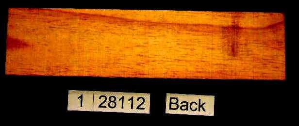
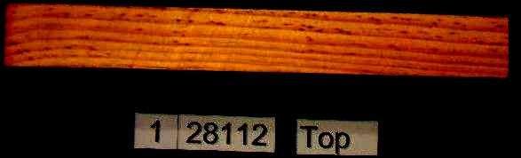
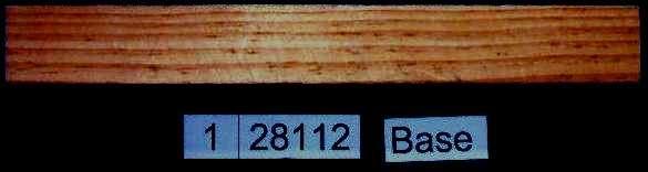
213 213 Appendix A

214 Sample 1 CT scan: Sample 2 CT scan: Sample 3 CT scan: 214

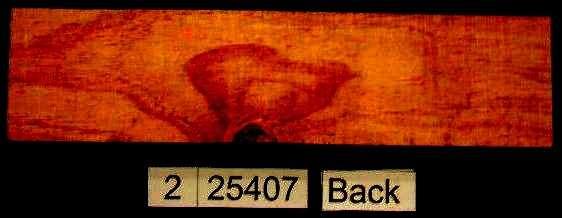
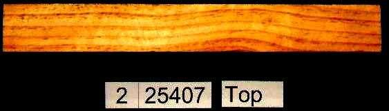
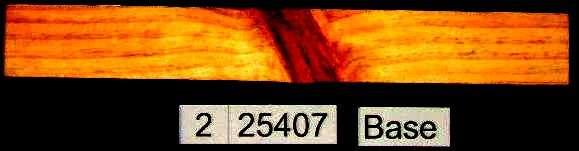
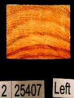
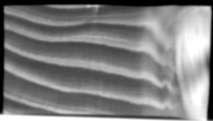
215 215

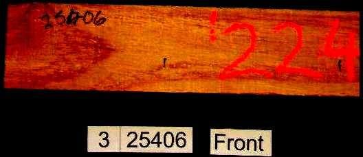
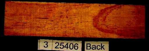
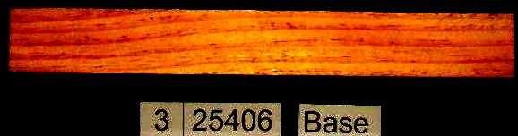
216 216

217 Sample 4 CT scan: Sample5 Sample 6 217

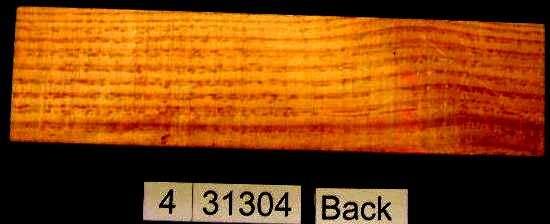
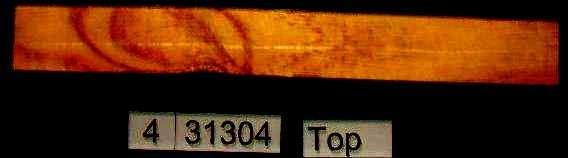
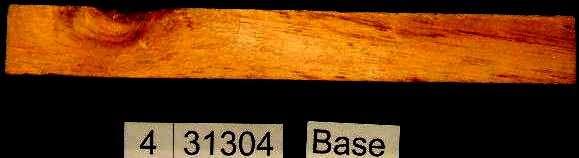
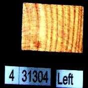
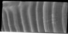
218 218

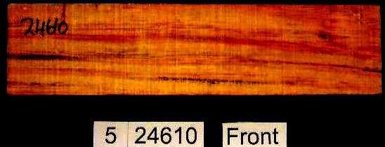
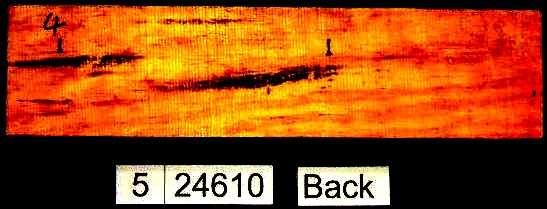
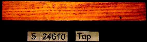
219 219

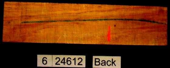
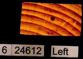
220 220

221 Sample 7: Sample 8: Sample 9: 221

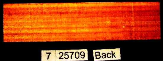
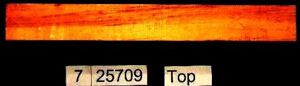
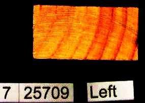
222 222

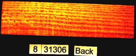
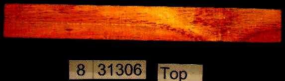
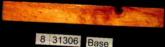
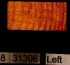
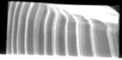
223 223

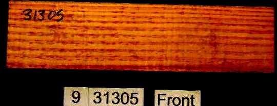
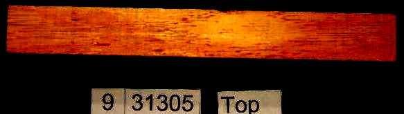
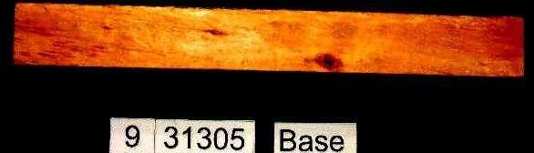
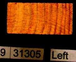
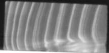
224 224

225 Sample 10 CT scan: Sample 11 CT scan: Sample 12 CT scan: 225

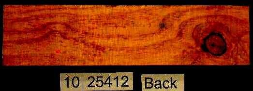
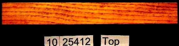
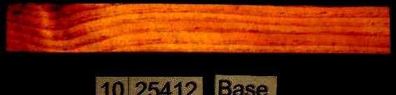
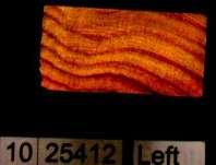
226 226

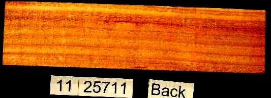
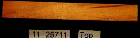
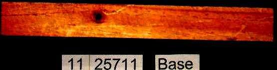
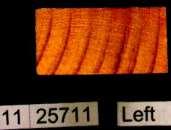
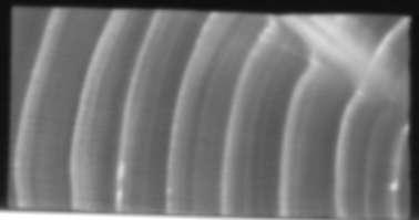
227 227

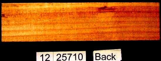
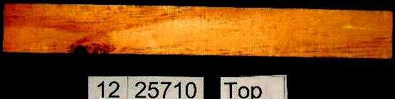
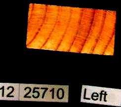
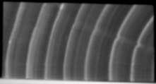
228 228

229 Sample 13 CT scan: Sample 14 CT scan: Sample 15 CT scan: 229

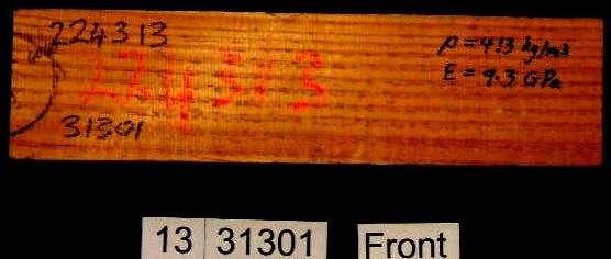
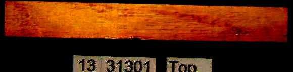
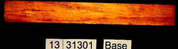
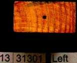
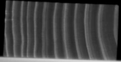
230 230

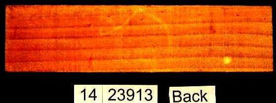
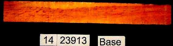
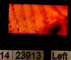
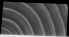
231 231

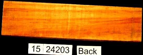
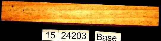
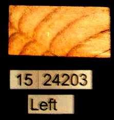
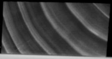
232 232

233 Sample 16 CT scan: S17 CT scan: 233

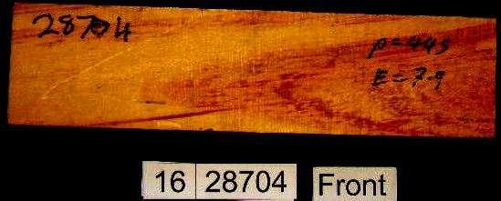
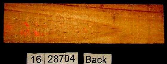
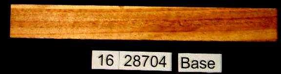
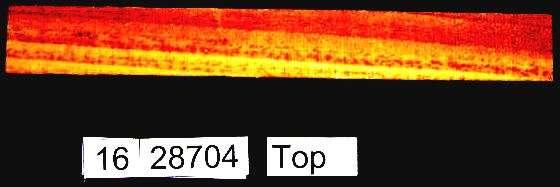
234 234

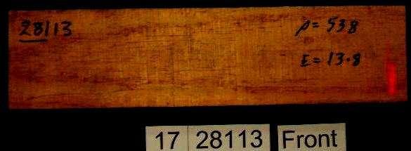
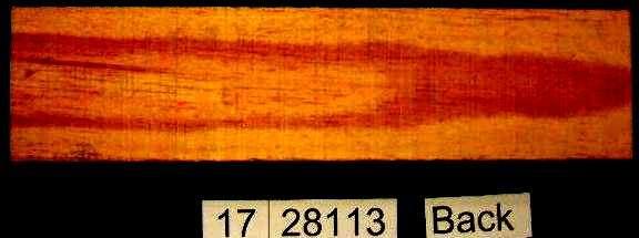
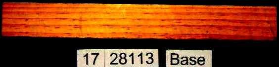
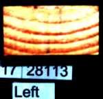
235 235

236 Sample 18 CT scan: Sample 19 CT scan: 236

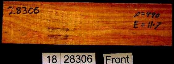
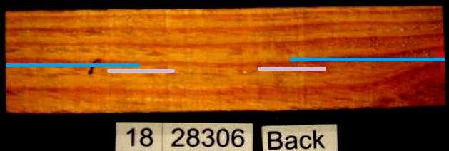
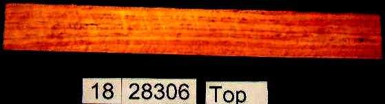
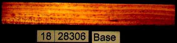
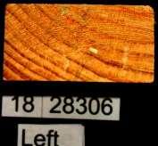
237 237

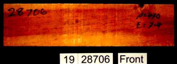
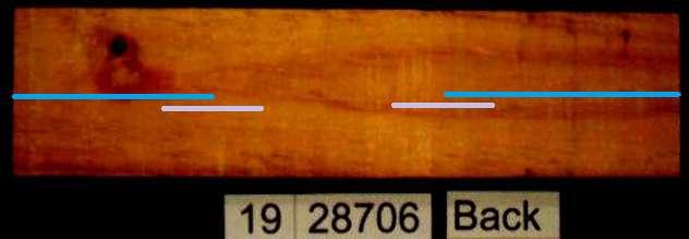
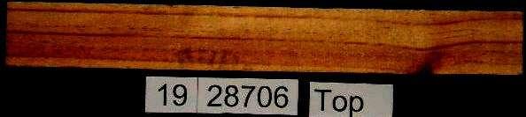
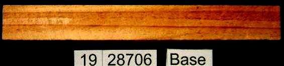
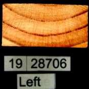
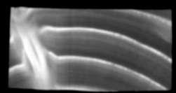
238 238

239 Sample 20 CT scan: Sample 21 CT scan: Sample 22 CT scan: 239

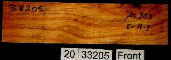
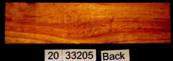
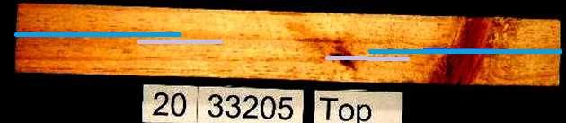
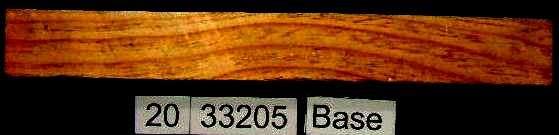
240 240

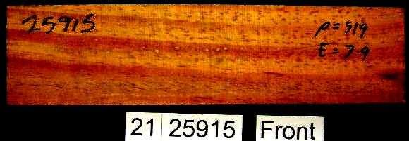
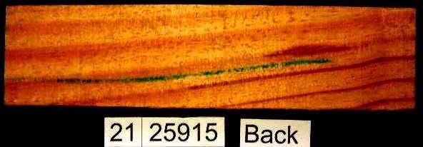
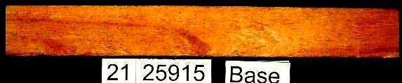
241 241

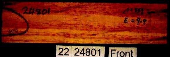
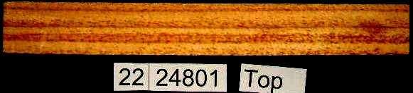
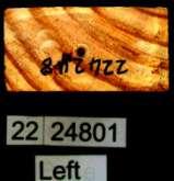
242 242

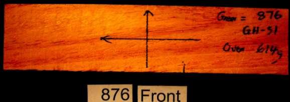
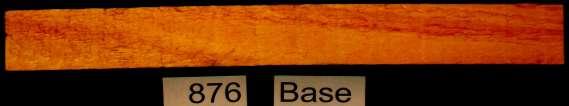
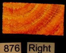
243 243 Appendix B

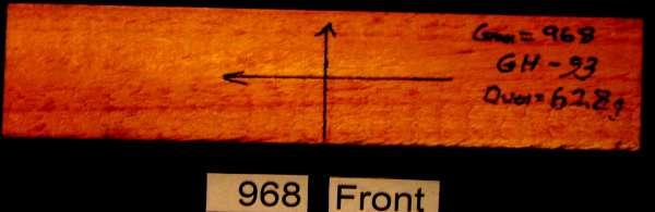
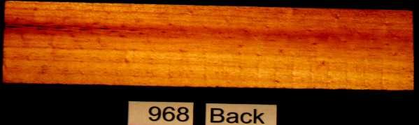
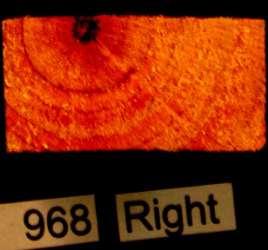
244 244

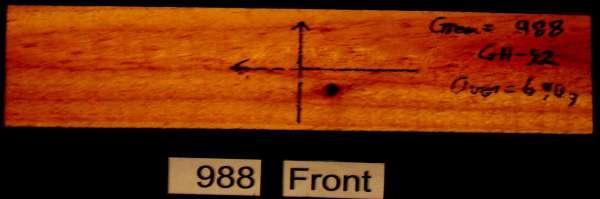
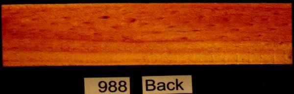
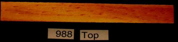
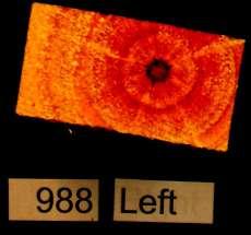
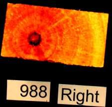
245 245

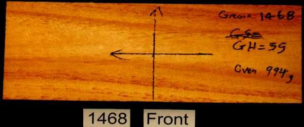
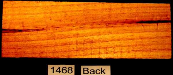
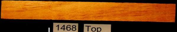
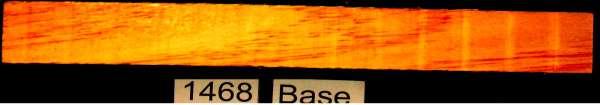
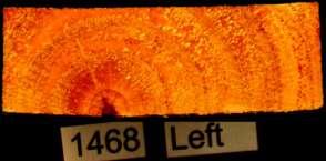
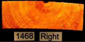
246 246

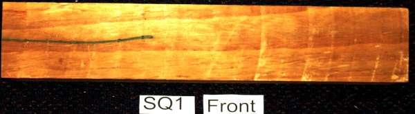
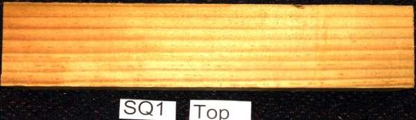
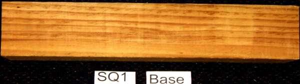
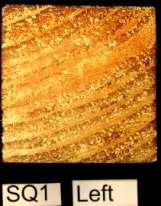
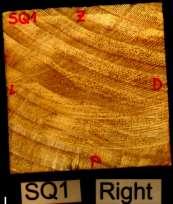
247 247

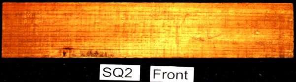
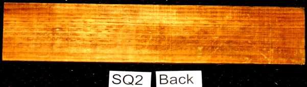
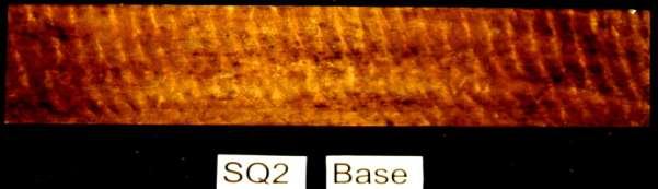
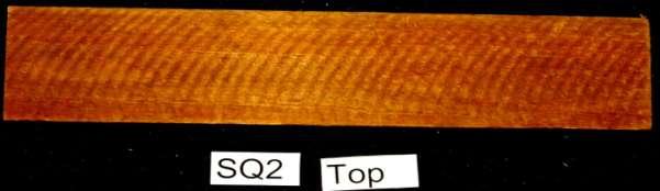
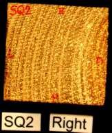
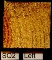
248 248

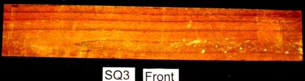
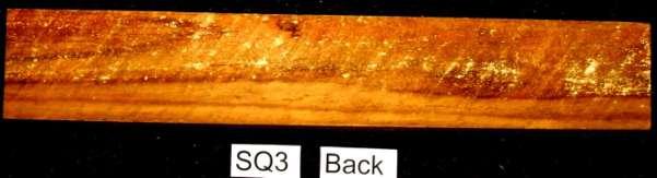
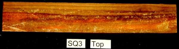
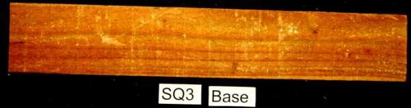
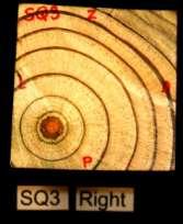
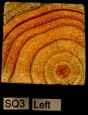
249 249