Correlation of Solar X-ray Flux and SID Modified VLF Signal Strength

Transcription

1 Air Force Institute of Technology AFIT Scholar Theses and Dissertations Correlation of Solar X-ray Flux and SID Modified VLF Signal Strength Shannon N. Kranich Follow this and additional works at: Recommended Citation Kranich, Shannon N., "Correlation of Solar X-ray Flux and SID Modified VLF Signal Strength" (2015). Theses and Dissertations This Thesis is brought to you for free and open access by AFIT Scholar. It has been accepted for inclusion in Theses and Dissertations by an authorized administrator of AFIT Scholar. For more information, please contact

2

3 The views expressed in this thesis are those of the author and do not reflect the official policy or position of the United States Air Force, Department of Defense, or the United States Government. This material is declared a work of the U.S. Government and is not subject to copyright protection in the United States.

4 AFIT-ENP-MS-15-M-077 CORRELATION OF SOLAR X-RAY FLUX AND SID MODIFIED VLF SIGNAL STRENGTH THESIS Presented to the Faculty Department of Engineering Physics Graduate School of Engineering and Management Air Force Institute of Technology Air University Air Education and Training Command In Partial Fulfillment of the Requirements for the Degree of Master of Science in Applied Physics Shannon N. Kranich, BS Captain, USAF March 2015 DISTRIBUTION STATEMENT A. APPROVED FOR PUBLIC RELEASE; DISTRIBUTION UNLIMITED.

5 AFIT-ENP-MS-15-M-077 CORRELATION OF SOLAR X-RAY FLUX AND SID MODIFIED VLF SIGNAL STRENGTH Shannon N. Kranich, BS Captain, USAF Committee Membership: Dr. William F. Bailey Chair Dr. Robert D. Loper Member Lt Col Robert S. Wacker, PhD Member Dr. Karatholuvu S. Balasubramaniam Member

6 AFIT-ENP-MS-15-M-077 Abstract This paper presents a quantitative comparison of the X-ray flux during solar flares, as measured by the GOES-15 satellite, and the associated effects on the ionization levels in the lower ionosphere as measured by Sudden Ionospheric Disturbance (SID) monitors around the globe. These monitors detect signals from a variety of different transmitting stations, each sending a unique Very Low Frequency (VLF) or Low Frequency (LF) radio wave signal ranging from 16.4 to 77.5 khz. Global signal propagation distances are achieved via the Earth-ionosphere waveguide propagation mode. During a solar flare, the increased X-ray flux enhances the ionization response in the sunlit ionosphere. The resulting SID in the lower ionosphere alters LF and VLF signal propagation. The monitored signal strength increases as a result of increased conductivity of the layer and a decrease in height of the ionosphere boundary. X-ray flux and SID modified signal strength were analyzed from March 2010 to June Ionospheric incubation times, and duration and strength of signal enhancement are related to flare strength via the X-ray flux enhancement. iv

7 Acknowledgments I would like to express my gratitude to my advisor Dr. Bill Bailey for his patience, and continual support and guidance throughout this process. I would like to acknowledge Ján Kárlovský and Lionel Loudet for their work with SID monitors, their excellent websites, and extensive data collection, without which this project would not have been possible. I would like to thank my family, especially my mom and dad, for their love, support, and encouragement. Lastly, I would like send my love and profoundest appreciation to my fiancé for sticking with me, sitting up with me on the late nights, and enduring the boring weekends keeping me company while I worked. In thanks, Shannon N. Kranich v

8 Table of Contents Page Abstract.. iv Acknowledgements.v List of Figures..viii List of Tables.ix I. Introduction..1-1 Motivation Background.1-1 Research Objectives 1-3 II. Background.2-1 Natural Phenomena..2-1 Solar Flares..2-1 The Ionosphere Sudden Ionospheric Disturbances.2-19 The Earth-Ionosphere Waveguide Mode Equipment GOES-15 and the XRS SID Monitors.2-29 III. Methodology..3-1 Data collection GOES-15 XRS Data 3-1 Stanford University Solar Center SID Monitor Program.3-3 AAVSO sites: Hlohovec Observatory and Southern France Data Processing.3-11 IV. Analysis and Conclusions Hlohovec Analysis Southern France Analysis 4-5 Conclusions.4-8 Future Work Appendix A: Stanford SID Monitor Database A-1 vi

9 Appendix B: Stanford SID monitors from map not found in database...b-1 Appendix C: Transmitter List.C-1 Bibliography...BIB-1 vii

10 List of Figures Figure Page 1-1 Work breakdown structure Electromagnetic emissions from the sun Two ribbon flare Geometric structure of a solar flare Snell s Law and the index of refraction in the ionosphere The Earth-Ionosphere Waveguide SID monitor signal examples Stanford SID monitor examples SID monitor block diagram GOES X-ray flux plot Stanford Solar Center SID Monitor SID monitor and VLF transmitter locations hour plot of x-ray flux and modified signal strength hour plot of x-ray flux and modified signal strength Hlohovec time of max VLF signal strength vs time of max X-ray flux Hlohovec VLF signal strength as a function of flare magnitude Modified Hlohovec VLF signal strength as a function of flare magnitude Southern France DHO signal strength as a function of flare magnitude DHO signal strength comparison between Hlohovec and Southern France Southern France seasonal comparison.4-8 viii

11 List of Tables Table Page 2-1 Hydrogen Alpha size classification Hydrogen Alpha intensity classification X-ray classification AFRL example data AFRL flare and VLF signal example data ix

12 CORRELATION OF SOLAR X-RAY FLUX AND SID MODIFIED VLF SIGNAL STRENGTH I. Introduction 1.1 Motivation The ionosphere greatly influences long wave radio transmissions and communications. During solar flares, there is a several order of magnitude increase in X- ray flux which rapidly increases photoionization in the lower ionosphere. This sudden change in ion density is known as a Sudden Ionospheric Disturbance (SID). Low Frequency (LF) and Very Low Frequency (VLF) radio waves, broadcast from point source transmitters around the world, are altered by the change in electron content of the low ionosphere. The increased conductivity and the lowering of the ionospheric boundary cause the radio wave amplitude to increase as seen when intercepted by a radio receiver. The study of signal enhancement was first conducted by the Cambridge Group in the late 1940 s [Bracewell and Straker, 1949]. Study of SIDs have continued through the decades, but little work has been done to compare the signal responses to the changes in X-ray flux. When this project was proposed by the Air Force Research Laboratory (AFRL), Dr. Balasubramaniam stated that this cross-disciplinary work is precisely what is missing and what is needed for the Air Force [Balasubramaniam, 2014]. 1.2 Background This study consists of a quantitative comparison of X-ray flux during solar flares as measured by the GOES-15 satellite and the associated effects on the ionization levels of the lower ionosphere as measured by SID monitors around the globe. GOES-15, in 1-1

13 operation since March 2010, is part of the Geostationary Operational Environmental Satellite (GOES) system operated by the National Oceanic and Atmospheric Association (NOAA). In the time since its launch, GOES-15 has recorded over 500 solar flares of M- class or greater by continuously measuring the changes in X-ray radiation flux incident upon the Earth s upper atmosphere. Before the dawn of the GOES satellites, flares were classified by measuring size and relative brightness on photographs taken using a Hα filter. Solar flares are now classified by the peak X-ray flux measured by the GOES satellite system, with M-class measuring between 10-5 and 10-4 watts per meter squared and X-class flares measuring greater than 10-4 watts per meter squared. In 2007, the Solar Center at Stanford University introduced a design for an inexpensive, yet effective, device that could be used to monitor SIDs. In conjunction with the United Nations Heliophysical Year, the monitors were designated for distribution to all 193 countries around the world. In addition, the American Association of Variable Star Observers (AAVSO) works with professionals across the world to maintain a SID monitoring network with privately built and maintained SID monitors. These monitors measure a variety of different transmitting stations from across the globe, each sending a unique Low Frequency (LF) or Very Low Frequency (VLF) radio signal ranging from 16.4 to 77.5 khz. These radio waves are able to propagate long distances by reflecting off free electrons in the ionosphere which constitute the upper boundary of the Earth- Ionosphere Waveguide. During a solar flare, the X-ray radiation hitting the Earth s atmosphere increases by as much as four orders of magnitude in a matter of minutes. The Total Electron Content (TEC) increases as the high frequency radiation ionizes the molecules of the ionosphere. The increased electron content, in turn, results in an 1-2

14 increased signal strength of the transmissions as the altitude and location of the signal reflection lowers with electron concentrations penetrating deeper into the normally neutral atmosphere. 1.3 Research Objectives Using the data gathered by GOES-15 and SID Monitors across the globe, this thesis examines LF and VLF signal response during SIDs as a result of increased X-ray flux from M-class and X-class solar flares, beginning in March 2010 and ending June 2014 (see Figure 1-1 below). During this project, a usable SID monitor database will be compiled for this and future research. This research will examine the magnitude of the change in radio signal strength recorded with respect to the change in the magnitude of X-ray flux as well as the seasonal variation of the ionosphere. Incubation times for the ionosphere to fully respond to increased X-ray flux, as well comparison of the rise time, duration, and decay time of the SID to the corresponding solar flare will be analyzed, as well as transmitter frequency dependence on SID signature. 1-3

15

16 II. Background This chapter discusses the background information necessary to understanding the major concepts addressed and the equipment used in the course of this research. The first part of this chapter begins with a discussion of the sun and an introduction of solar flares, then it progresses to Earth s upper atmosphere to discuss the basics of the ionosphere and sudden ionospheric disturbances (SIDs), and lastly it discusses propagation of electromagnetic waves through the neutral atmosphere and how the ionosphere affects that motion. The second part of this chapter addresses the equipment used to collect the data including the GOES15 satellite and the SID monitors. 2.1 Natural Phenomena Solar Flares Solar flares are the most explosive events in the solar system, ejecting electromagnetic radiation, energetic particles, and stellar material into space. Solar flares occur when the magnetohydrodynamic equilibrium of the sun s magnetic field is disturbed, causing a rapid and violent release of energy stored in the magnetic field lines [Foukal 2013]. Solar flares are capable of releasing up to Joules of energy and kilograms of mass over time spans of seconds to just a few minutes [Acebal 2013]. The radiation and plasma emitted into the interplanetary medium during these events play a major role in space weather. Space weather encompasses all interactions between the Earth s magnetic field, its atmosphere, and interplanetary space. Electromagnetic radiation constantly irradiates Earth at an average rate of 1360 watts per square meter, which is known as the solar constant. Forty-one percent of this radiation lies within the visible spectrum detectable by 2-1

17

18 and Environmental Research Inc. found that if similar event were to happen today, the economic costs to the United States alone would be between trillion USD due to loss of transformers and electrical circuits, causing widespread power outages lasting weeks to years [Lloyd s 2013]. Nationwide loss of transformers due to power surges would take years to fully recover. A study published in early 2014 concluded that the probability of a similar event occurring in the next ten years to be 12 percent [Riley 2012]. The first major advancement in solar flare observation didn t come for over 80 years, until World War II, when British radar operators observed radiation of an unknown origin. When the reports were released in 1945, a new field of study emerged known as radio astronomy, which focused on categorizing solar radio signals [Foukal 2013]. With Earth s atmosphere blocking the majority of extreme ultraviolet (EUV) and X-ray radiation, it was not until the space age that the true complexity of solar flares began to reveal itself. The first observations of EUV and X-ray emissions were completed by the Naval Research Laboratory in the late 1940s using rockets developed during World War II. Since that time, satellites and space stations have made tremendous advances in solar observations. Studies of the electromagnetic radiation released by solar flares have provided knowledge of flare phases and flare types leading to the development of two systems for classifying solar flares. Additionally, understanding of flare structure and development has led to knowledge of how and where in the solar atmosphere specific wavelengths of radiation originate. Observing the electromagnetic emissions from the sun has allowed astronomers to identify three main phases of a solar flare; the pre-flare, the impulse or flash, and the 2-3

19 decay (see Figure 2-2 below). Solar flares occur in regions of high magnetic activity above the surface of the sun. These active regions are most notably marked in the visible spectrum by sunspots on the sun s surface and can be seen in the X-ray and EUV portions of the electromagnetic spectrum as bright patches relative to the quiet background of the solar disk. During the pre-flare phase, there is a noticeable brightening of the active region in the X-ray and EUV portions of the spectrum as the magnetic field lines become unstable. This phase usually lasts only a few minutes, but can last for several hours in some cases [Foukal 2013]. The most energetic part of the flare occurs during the flash, or impulsive phase, and produces the greatest increase in radiation output. The flash phase lasts seconds to minutes with individual impulses lasting seconds or less. In these moments, emissions in the X-ray, EUV, microwave, and Hydrogen-alpha (Hα, Å) portions of the electromagnetic spectrum reach their maximum and are used by astronomers to mark the precise timing of the flare event. Following the flash phase the decay phase begins, marking the gradual decrease of flare radiation to levels before the pre-flare stage, or to levels comparable to the background emissions from the rest of the solar disk. During the decay phase, strong magnetic regions may continue to release multiple flares, compounding the total emissions and increasing the length of the decay phase to as long as several days. 2-4

20 Figure 2-2. Consecutive Hα images of a two ribbon flare, noted by the two bright lines on either side of the darker central neutral zone, in pre-flare (frames 1-3), impulse (frame 4), and decay (frame 5-6) stages taken by Big Bear Solar Observatory, 29 April The pattern in which radiation emerges can also tell astronomers about the type of solar flare. Solar flares are generally categorized as compact flares or two-ribbon flares [Foukal 2013]. Compact flares are marked by a brightening within a magnetic loop above the sun s surface. These flares are small, lack the energy to accelerate solar material to escape velocities, and cause little to no structural change in the magnetic field lines. Without the energy needed to project plasma into space, these flares have little to no impact on space weather or Earth s environment. Two-ribbon flares however, are the spectacular, explosive, events most commonly thought of in association with solar eruptions. These events are marked by a brightening of two narrow strips along 2-5

21 oppositely-polarized magnetic field lines on either side of a magnetic neutral zone (see Figure 2-2 above). These events occur in the breaking and recombining of magnetic field lines and cause large scale changes in the magnetic field surrounding solar active regions. The strongest of these events can accelerate solar material at near relativistic speeds creating shockwaves both in the stellar atmosphere and through interplanetary space. The radiation and material released from two-ribbon flares create far-reaching impacts and can have devastating impacts on Earth s environment and technology. Astronomers further classify flares using radiation emissions in the visible or the X-ray portions of the electromagnetic spectrum. The first classification system, developed in the 1930 s, was the Hα Classification. Hα classification uses a series of images taken by cameras filtered to the Hα emission line at Å. The Hα line lies in the visual portion of the electromagnetic spectrum, and is part of the Balmer series. The light seen at this wavelength is the emission seen when a photon is created in the decay of Hydrogen atoms from the third excited state to the second. Using images of the sun, the system uses two criteria to classify a flare: total size and relative brightness. If a chromospheric brightening exceeds 300 million square kilometers it is assigned a value from 0 to 4 and is measured in square meters, or in millionths of the solar disk at the time of maximum brightness (see Table 2-1 below) [Foukal 2013]. The brightness is then categorized as F, N or B, representing faint, normal and brilliant, to describe the intensity of the flare relative to the rest of the solar disk (see Table 2-2 below). Due to differences in human perception and the subjective nature of the criteria, this system is not as reliable or consistent as the newer system of classification. 2-6

22 Table 2-1. Hydrogen Alpha Size Classification Flare Area Flare Area Flare Importance Millionths of the Solar Hemisphere Square meters 0 <100 <2.48x x x x x x x >1200 >3.06x10 8 Table 2-2. Hydrogen Alpha Intensity Classification Brightness Percent of Background Faint 160% - 270% Normal 270% - 360% Brilliant >360% The X-ray classification system that replaced the Hα system is based on the maximum soft X-ray, or 1 to 8 Å wavelength, flux as measured in watts per square meter by the GOES satellite systems. This system has been in place since 1974 with the launch of the first geostationary meteorological satellites. The system classifies solar flares with a letter designator of A, B, C, M, or X, with A being the weakest flares and X the strongest (see Table 2-3 below). A and B class flares are not strong enough to impact Earth s environment or satellites and are often too weak to even be detectable at Earth orbit. C class flares are the most common type of flares observed from Earth orbit and by ground-based instruments. However, these flares are still too weak to have any major impact on Earth environment or operations. M stands for medium or moderate intensity and can have noticeable impacts on global positioning, satellite communications, and radio signals. The largest flares fall under the X classification for their extreme nature and potential impacts on Earth. 2-7

23 Table 2-3. X-ray Classification Letter Designator Peak X-ray Flux (W/m 2 ) A <10-7 B C M X >10-4 X class flares have enough power that, if directed toward Earth, could disable satellites, disrupt long range communications, and fail entire power grids. Flares within each category are given a numerical sub-category. The scale is logarithmic with each numerical class of flare having ten times greater peak X-ray flux, than the previous class. Since the highest classification is X, an exception has been made in the numbering system to allow flares higher than X9. The largest recorded flare to date was an X45 on 4 November 2003, and while powerful enough to have destroyed Earth s satellites, power grid, and the economy, the planet narrowly avoided the stream of deadly particles and radiation released by this storm. [Thomson 2004]. The X-ray classification system, based on precise timing and measurements by standardized equipment, will be the system used and referenced for the duration of this research. The introduction of space-based observations has provided an understanding of the structure and mechanics of a solar flare. The distinct processes of how a flare occurs, how the radiation is produced, and how the energy is released are important aspects in understanding and, possibly, accurately predicting solar flare events. The current understanding of flare dynamics begins with the interweaving of the complex network of 2-8

24 magnetic field lines arching in and out of the solar surface. It is possible for the field lines to become so tangled that they snap and recombine in a powerful release of energy (see 1 in Figure 2-3 below). The reconnection of the magnetic field lines creates the flash of the solar flare and corresponds to the most massive release of X-ray and EUV radiation during the flare event. Solar plasma is accelerated both back toward the sun s surface and away from the sun creating radio bursts (see 2 in Figure 2-3 below). If accelerated fast enough, the plasma may escape the sun s gravity and launch into interplanetary space creating coronal mass ejections (CMEs) and energetic proton events (see 3 in Figure 2-3 below). Particles that do not escape, or that are accelerated back toward the sun, can become caught in the new magnetic field lines. These particles release radio gyrosynchrotron radiation, which is caused by the direction of the charged particles motion changing as they spiral along the new magnetic field lines. Particles forced downward from the upper parts of the solar atmosphere rapidly encounter the higher densities of the lower atmosphere, producing Bremsstrahlung in the X-ray and radio as particles slow and deflect during interactions with like charges (see 4 in Figure 2-3 below). Energy trapped by the new magnetic field lines near the base, or footprints, of the flare creates heating of the plasma near the sun s surface, causing it to rise. The plasma follows paths between the new field lines known as flux tubes creating a flare loop (see 5 in Figure 2-3 below). The heating and cooling of the plasma as it rises and falls within these tubes produces soft X-ray and EUV emissions. Additionally, some particles get trapped in the upper atmosphere of the sun, becoming part of new coronal loops (see 6 in Figure 2-3 below). Particles that fall into this path emit soft X-rays and radio emissions as they alter their directions and spiral around these altered field lines. 2-9

25 Figure 2-3. Geometric Structure of a Solar Flare. Adapted from Fig. 1 [Holman 2012] Reproduced with permission from Holman, Gordon D. Solar Eruptive Events, Physics Today, (April 2012). Copyright 2012, AIP Publishing LLC. There are four major outcomes from a solar flare: proton events, CMEs, nuclear reactions, and electromagnetic radiation emissions in the X-ray and EUV regions of the spectrum. Proton events are streams of highly energetic particles accelerated away from the sun by flares or CMEs. If these protons enter the Earth s magnetic field they can disrupt the charges already present and create new and potentially powerful electrical currents in the near-earth environment. The radiation and currents are hazardous to spacecraft and can be especially harmful to humans in orbit. The effects in the ionosphere 2-10

26 are seen when protons spiral toward the magnetic poles exciting particles in the atmosphere which emit photons when they relax to their neutral state. CMEs are massive bursts of solar wind and plasma accelerated to relativistic speeds, creating shockwaves in the ambient solar wind that ripple through the solar system. The plasma released by CMEs often carries its own magnetic field, which can cause distortion of any other magnetic field it comes in contact with. CMEs are the cause of geomagnetic storms that disrupt the magnetosphere and ionosphere. The most noticeable impact of these geomagnetic storms is the aurora, which occurs when electrons spiral along magnetic field lines toward polar regions, emitting UV and visible light when electrons interact with and excite the atoms and molecules in the atmosphere. As the particles return to their pre-excited state, they release photons. The diverse colors result from the unique emission spectrum of each type of molecule. The atmospheric currents caused by the electrons entering the atmosphere during these events can create power surges and have the potential to cause widespread power outages. The third type of event caused by solar flares is the nuclear reactions that send gamma ray bursts away from the sun. Gamma rays are the most energetic emissions from the sun. These emissions create problems both in orbit and in the upper regions of the atmosphere. The X-ray and EUV radiation can penetrate the ionosphere and reach the neutral atmosphere, increasing ionization through a process known as photoionization, effectively lowering the boundary of the ionosphere. The rapid ionization of the upper regions of the neutral atmosphere by X-ray radiation is one cause of sudden ionospheric disturbances, and will be the main focus of this research. 2-11

27 2.1.2 The Ionosphere The ionosphere lies in the uppermost region the Earth s atmosphere, in which there is always a nonzero concentration of ionized particles. The lower boundary of the ionosphere is approximately 90 km above sea level. The upper regions of the atmosphere are constantly bombarded by solar radiation and energetic solar wind particles. When the neutral molecules of the atmosphere absorb photons or are impacted by high energy particles, energy is transferred, increasing the kinetic energy of the neutral particles. When enough kinetic energy is transferred, neutral particles may be promoted to excited states, or ionized. Widespread ionization leaves behind a plasma that is approximately neutrally charged with near equal quantities of both positive and negative charges. This plasma exhibits a collective behavior governed by outside electric and magnetic fields. The study of plasma in Earth s ionosphere, dominates a large portion of the study of space weather. Just as the motions of the neutral atmosphere define terrestrial weather, the study of plasma movements defines ionospheric weather. There are three major motions associated with ionospheric plasmas: gyrating motion around magnetic field lines; oscillatory motion along magnetic field lines from north to south; and a drifting motion as particles proceed zonally in orbit around the planet. During solar flares and other solar events, the magnetic field of the Earth is disturbed and compressed, increasing its intensity. The plasma in the upper atmosphere is subsequently disturbed as the charged particles react to the changing magnetic field. Maxwell s equations tell us that these results will have rippling effects -- changing magnetic fields create new electric fields, moving particles create electrical currents, and changing electric fields and currents 2-12

28 create new magnetic fields. The series of reactions that take place after a solar event, until the atmosphere returns to a quiescent state, are known as geomagnetic storms. The other major component in ionospheric physics is the continual production and loss of ions and electrons. The main production mechanism of charged particles in the ionosphere is photoionization, which takes place when photons are absorbed by atoms or molecules that transfer enough energy to the electrons of the particle to exceed the ionization energy of the system. Photoionization is described by the chemical equation: X + photon X + + e (2-1) Where X is any atomic or molecular species in the upper ionosphere. The ionization energy for the reaction is the energy required for an electron to escape the electromagnetic bonds holding it to the nucleus. The rate of ion production of a particular atomic or molecular species can be described, by the Chapman production function: P c (z, χ) = I exp[ Hn(z)σ a sec χ]ησ a n(z) (2-2) In this equation, z refers to the height above sea level, χ is the solar zenith angle, I is the unattenuated flux of the desired wavelength measured at the top of the atmosphere, H is the neutral gas scale height (the characteristic length at which the absorbing species decreases density exponentially with altitude), n is neutral number density of the absorbing species, σ a is the absorption cross section for the absorbing species for the given wavelength of light, and η is the probability that photon absorption will result in an ion-electron pair [Schunk and Nagy 2009]. The neutral gas scale height depends on the temperature and mass of the species: H s (z) kt s (z) m s g(z) (2-3) 2-13

29 where the subscripted s indicates which species is being analyzed, z again denotes the height above sea level, T s (z) is the temperature of the species at the indicated height, m s is the atomic or molecular mass of the species, and g(z) is the force due to gravity at the desired altitude. The neutral number density n(z) is also further defined using the equation: n s (z) = n s (z 0 )exp (z z 0 ) H s (2-4) Where z 0 is a reference height where the density is already known and z is the height where the density is unknown. Understanding the Chapman production function shows that ion production is proportional to the intensity of incoming solar radiation, which is a maximum at the top of the atmosphere, and the density of the atomic or molecular species, which is a maximum at the bottom. A balance of these two is achieved at a height, z max, which is defined as: z max = z 0 + H ln[n(z 0 )Hσ a sec χ] (2-5) As seen in this equation, the height of maximum photoionization is dependent on the angle of the sun and is a maximum when the sun is at its peak. To find the total ionization rate, incoming radiation intensity and the absorption cross-section for each species must be integrated across all wavelengths and the production functions must be summed together for each species present at the desired altitude. Solar storms, particularly solar flares, rapidly increase the amount of energetic radiation hitting the top of the atmosphere, which rapidly increases the rate of ionization. This swift ionization of the ionosphere is classified as a sudden ionospheric disturbance and is the main focus of this research. 2-14

30 Other sources of ion production include secondary ionization, particle exchange and particle precipitation. Secondary ionization occurs when electrons emitted during photoionization have enough kinetic energy to be able to ionize a neutral particle themselves. While particle exchange is a source of ion production, it also results in the loss of an ion, leaving the overall ion density the same. Charge exchange is a basic transfer of an electron from one particle to another, generically described by: X + Y + X + + Y (2-6) Here, X and Y represent two different atoms or molecules. Particle precipitation is a consequence of energetic particles entering the atmosphere, and is particularly important in the upper regions of the ionosphere. High-energy electrons incident from the solar wind enter the upper ionosphere with enough energy to knock bound electrons free from their parent nuclei. This reaction can be written as: X + e incident X + + e incident + e released (2-7) Where X is again any atomic or molecular species present in the upper atmosphere. While these processes play a role in ion production, photoionization remains the main source of energy and ionization throughout all layers of the ionosphere [Prölss 2004]. As the ionosphere remains relatively stable, and is able to return to quiescent conditions after a storm, it is obvious that there are also sources of ionization losses. The main sources of ion loss are dissociative recombination, radiative recombination, and charge exchange. Dissociative recombination is the most important loss process for molecular ions. In this process an ionized molecule absorbs an electron and separates into its constituents, forming two neutral atomic species. This process is described by the generic reaction: 2-15

31 XY + + e X + Y (2-8) Radiative recombination is the predominant loss process for atomic ions. In this process, an atomic ion recombines with a free electron and excess energy from the reaction is expended as radiation. X + + e X + photon (2-9) As this reaction consists of two particles combining into one, there is a very precise combination of energy and momentum transfer required to satisfy conservation laws making this reaction extremely rare in comparison to dissociative recombination. Charge exchange was previously discussed in the context of ion production. While this process results in the loss of a particular ion species, it does not affect the ion density of the ionosphere as a whole. While there are several production and loss processes in the ionosphere, the most important is photoionization. As seen from equations (2-2) through (2-5), altitude plays an important role in photoionization and thus the characteristics and behavior of the ionosphere. Earth s ionosphere is divided into three distinct altitude regions: the D region, between 70 and 90 km above sea level; the E region, between 90 and 150 km; and the F region, between 150 and 1,000 km. During the day, the F region is further divided into two layers, F1 and the F2. The F2 layer extends from 200 to 1000 km and at night, assimilates the lower F1 layer through recombination, dropping its lower boundary to approximately 150 km. The F2 layer contains the highest electron density in the ionosphere, as heavier particles are trapped at lower altitudes by Earth s gravity. The most common ions in the F2 region are atomic oxygen (O + ). At the highest altitudes, above 800 km, O + gives way to hydrogen (H + ) and helium (He + ) ions as the ionosphere 2-16

32 meets the boundary of, and merges into, the plasmasphere [Prölss 2004]. The majority of ions in the F1 layer are nitrous oxide (NO + ) and O +. Since molecular ions are 10 5 times more likely to recombine with an electron than atomic ions; without the ionizing radiation from the sun to maintain ionization levels, NO + recombines with the available electrons and return to its neutral state [Knipp 2011]. This recombination of NO + makes the F1 and F2 regions indistinguishable at night merging the two layers into a single F region. The high electron density in the two F layers plays an important role in long range communications having the greatest impact on high frequency (HF, 3 to 30 MHz), radio wave propagation. This research will measure the ion and electron densities in each layer using radio wave propagation. The E region was the first of the three ionosphere layers to be discovered, by Appleton and Barnett. The region was designated E for the reflected electric field they found during their investigation of downward waves via atmospheric interference [Appleton 1925]. The major ions in this region are molecular oxygen (O + 2 ), molecular nitrogen (N 2 + ) and NO + [Schunk and Nagy 2009]. The E layer is highly variable, dependent on diurnal, annual, and cyclic solar activity. The E region has highest ion concentrations during daylight hours, summer months, and solar maximum, the peak of the eleven year sinusoidal rise and fall in total solar activity. While strongly ionized during the day, recombination rates at night can cause the ionization of this layer to decrease dramatically. When daytime radiation levels are low during solar minimum or during winter months, the E region may disappear entirely in the hours before sunrise. This region best reflects radio frequencies below the HF range, but at times of high 2-17

33 ionization, can reflect frequencies into the Very High Frequency (VHF, 30 to 300 MHz), spectrum. The D region is the most important to this research. It interacts heavily with the neutral atmosphere below. Due to high neutral particle density and high collision rates between electrons, ion, and atoms and molecules, this region disappears within minutes after the sun sets. The dynamic nature of this layer make it the most difficult to study and understand. X-ray and EUV radiation play the dominant roles in the ionization of the D region, with X-rays being strong enough to ionize all atmospheric gases and EUV predominantly ionizing O and N [Knipp 2011]. The most notable feature of the D region is that it contains negative ions as well as positive. The primary positive ions found in this layer are molecular O 2 and NO, and the primary negative ions are nitrate (NO - 3 ). N 2, N, O, and H 2 O molecules also play important roles in the chemical composition of this layer. During solar flares, when X-ray and EUV emissions increase exponentially, so does the ionization of the D region. During strong solar events, ionization penetrates into the neutral atmosphere, lowering the boundary of the D region to as low as 50 km. The changing height of the D layer has noticeable impacts on the waveguide mode and the long range propagation of low frequency (LF, 30 to 300 khz), and very low frequency (VLF, 3 to 30 khz), radio waves through the atmosphere. This paper will focus on propagation of LF and VLF radio waves, specifically those between 16.4 and 77.5 khz. It will also address the changes in signal strength as the height of the ionosphere varies with ionization levels. 2-18

34 2.1.3 Sudden Ionospheric Disturbances A sudden ionospheric disturbance (SID) is defined as a rapid increase in the ionization density [Prölss 2004]. While SIDs are commonly associated with the D region, enhancements can be seen in all layers of the ionosphere. The dramatic surge in EUV and X-ray emissions associated with solar flares creates increased ionization in all three layers of the ionosphere. This response happens within minutes with the onset of increased radiation flux, while the decay times vary with altitude. The lower ionosphere s decay is follows the same pattern as the radiation flux enhancements, while the upper ionosphere can take significantly longer for normal ionization levels due to the lower recombination rates [Mitra 1974]. It has been shown that X-ray emissions play the dominant role in the photoionization of the lower (D and E) regions of the ionosphere while EUV has a more dramatic impact at higher altitudes in the F regions [Tripathi 2011]. The difference in ionization based on wavelengths logically stems from the fact that the H and He atoms in the upper ionosphere have lower ionization energies than the heavier atoms and molecules, such as O and N, which predominate in the lower ionosphere [Prölss 2004]. While SIDs affect the entire ionosphere, their effects on the D region and neutral atmosphere are most apparent due to the disruption of long-range radio communications. X-ray radiation greatly increases the ionization levels and electron density of the D region and upper levels of the neutral atmosphere, effectively lowering the boundary of the ionosphere. As the upper regions of the neutral atmosphere experience enhanced ionization, the electron density becomes comparable to that of the unenhanced D region. This lowering of the ionospheric boundary affects both high and low frequency radio transmissions. SIDs are characterized by the increased concentration 2-19

35 of ions and electrons throughout the ionosphere and how they change the behavior of the D region for a short period of time. SIDs are categorized by the radio frequencies affected by the ionospheric changes. Low-frequency waves are typically reflected by the electrons in the D region of the ionosphere, while mid- and high-frequency waves have enough energy to propagate through the D region. High-frequency radio waves reflect off of the E and F regions where the electron content is higher. Depending on the frequency of the wave and how its amplitude, frequency, and phase are affected, one of six classifications can be used to describe the perturbations. Disturbances to low-frequency waves include sudden enhancements of atmospherics (SEAs), sudden enhancements of signal (SESs), and sudden phase anomalies (SPAs). Disturbances to high frequency systems are short-wave fadeout (SWF), sudden frequency deviation (SFD), and sudden cosmic noise absorption (SCNA). The changes created by SIDs to the lower ionosphere and the resulting effects on LF and VLF radio transmissions due to the increased electron content will be the focus of this research. LF and VLF frequencies are most often used for long-range communications, especially by the military. A variety of low-frequency signals, both natural and manmade, propagate through the atmosphere. The first type of SID event effecting natural VLF signals is a SEA. Lightning strikes produce a continuous spectrum of LF and VLF radio waves. During SEA events, these naturally-occurring radio waves are enhanced by the increased reflectivity of the heightened electron content in the D region. The effect of this are most commonly heard as static in the background of radio speakers [Knipp 2011]. 2-20

36 SPAs affect manmade signals originating from the surface. These radio waves reflect off the ionosphere and return to the surface beyond the horizon, making long range communications possible. An SPA is the sudden phase shift of a VLF wave caused by the decrease in height of the D region boundary, which alters the altitude of reflection of the wave, and may prevent it from being received at the intended location [Knipp 2011]. SES events are similar to SEA events, except for man-made point sources rather than the natural, widespread signals. In this type of event the amplitude of the VLF wave is heightened, increasing the signal strength at the receiving station. These events mark clear signal responses that mirror the rise and fall of the total electron content in the lower ionosphere. This research focuses on SES events, measuring the changes in the amplitude of LF and VLF signals from transmitters around the world. High-frequency radio waves are also affected by sudden ionospheric disturbances, but unlike LF and VLF signals, HF and VHF signals are absorbed rather than of enhanced. SWFs occur in which there is a sudden decrease in the received signal strength. This phenomenon was first observed in the 1930s by Hans Mögel, a German physicist working for Transradio in Berlin [Mitra 1974]. This type of event causes degradation of received signals or, in extreme events, loss of the radio signals entirely. HF and VHF waves have enough energy to propagate through the D region, and are most commonly reflected off of the E and F regions of the ionosphere. During a SID, with the increased ionization in the D region, HF and VHF radio waves are partially or fully attenuated as they pass through this layer, both on the way up and again on the return trip 2-21

37 downward. If the signal survives both passes through the enhanced D region, the signal that reaches the receiver will be severely diminished. SFDs usually affect transmissions that reflect at altitudes greater than 100 km [Mitra 1974]. Waves that would usually reflect off the F1 or F2 region will experience a sudden shift in frequency when the electron content in a lower region becomes high enough to reflect the waves sooner than expected. This early reflection causes a Doppler shift in the frequency of the wave resulting in missed transmissions with receivers looking for the wrong signal [Knipp 2011]. SCNAs affect radio waves originating from stars and galaxies across the universe. Cosmic waves typically lie in the HF range around 20 MHz creating a constant background noise for receivers looking toward space. During SCNA events, the heightened electron content in the D region absorbs this radiation before it can reach Earth s surface, diminishing or negating the usual signal. All SID events are dependent on the photoionization of neutral atoms and molecules to create a sudden increase in total electron content (SITEC) within the ionosphere. Photoionization requires the increased radiation from the solar flares to be directly incident on the ionosphere, so SIDS are exclusively a daytime phenomenon. Despite this limitation, SIDs are one of three ground-based observation techniques (the others are Hα imaging and radio burst monitoring) for identifying and studying solar flares, and they play a vital role in the study of solar flare emissions and ionospheric chemistry. The most common technique for studying SIDs is to monitor LF and VLF transmissions through ground-based receivers for fluctuations in signal strength or frequency. Transmitters broadcasting on a single, steady radio frequency have been 2-22

38 established worldwide by military and emergency management agencies. These signals can be monitored with an appropriate radio receiver. The American Association of Variable Star Observers (AAVSO) maintains a global network of ground-based observers monitoring SIDs continuously. AAVSO members and their archive of publicly accessible data was invaluable to this research The Earth-Ionosphere Waveguide Mode While enhancements to the total electron content (TEC) can be seen in all regions of the ionosphere, SID effects are most important in the D region, which has the greatest impact on radio communications. During the day, the D region forms the upper boundary of the Earth-ionosphere waveguide. A waveguide is formed by two boundaries through which electromagnetic waves are passed along a sinusoidal path, bouncing between the confining media. The Earth and ionosphere act as two approximately parallel conductors at an average of 80 km apart, which create a waveguide mode for radio waves with wavelengths of several km or less [Budden 1961]. The waveguide mode enables longrange communication by propagating signals that would otherwise be restricted to lineof-sight distances. The first instance of long-range communication occurred in 1901 when radio signals were first successfully transmitted across the Atlantic Ocean [Schunk and Nagy 2009]. Initial theories of long-range propagation included diffraction around only one conducting surface, but it was soon proven in that this method could not provide enough strength to perpetuate the signal over the distances achieved. In 1902, the existence of a layer of electrically charged particles in the upper atmosphere was proposed as the source for the additional conducting surface [Schunk and Nagy 2009]. The existence and height of this layer was later confirmed in

39 While the Earth and ionosphere can roughly be considered concentric spheres, it is customary, for a basic understanding of waveguide modes, to ignore curvature and treat both surfaces as planer. A second simplifying assumption is to treat the ionosphere as a sharply defined boundary at a fixed height. This boundary is defined by a change in the index of refraction, n, between the atmosphere and ionosphere. The refractive index is the ratio of the speed of light in a vacuum to the speed of light in a medium. The index of refraction for Earth s atmosphere is In a plasma, such as the ionosphere, the refractive index, in SI units, is defined by: n = 1 N ee 2 ε 0 m e ω N e f 2 (2-10) Where N e is the electron density, e is the charge on an electron, ε 0 is the permittivity of free space, ω is the angular frequency, and f is the wave frequency of the incident electromagnetic wave [Knipp 2011]. As seen from equation 2-10, as the electron density increases, the index of refraction decreases. When a wave encounters a variation in refractive index between two media, it is refracted, or bent. A higher refractive index indicates a greater refraction of the wave (see Figure 2-4 below). The angle of refraction at the boundary between two media is defined by Snell s Law: n i sin θ i = n r sin θ r (2-11) In this equation n i is the index of refraction for the medium the wave starts in, θ i is the angle of incidence, n r is the index of refraction for the refracting medium, and θ r is the angle at which the wave is refracted. When θ r 90, the wave is reflected instead of refracted, so that the wave returns to the original medium instead of proceeding to the next. The electron content of the ionosphere determines its index of refraction and 2-24

40 therefore the propagation path. When plasma density is enhanced, the propagation path is altered and signal amplitude effected. n 2 θ 2 N e2 n 1 θ 1 N e1 n 0 N e0 θ 0 Figure 2-4. Electron density, N e, increases with altitude, index of refraction, n, decreases with altitude, which increases the angle, θ, at which a wave is deflected from the vertical. When the angle of refraction angle reaches 90 degrees, the wave is reflected off the ionosphere and returned to Earth. Previously, the ionosphere was assumed to be a sharp boundary. This is obviously not true, as electron density changes diurnally as well as seasonally and during any space weather events. Even on a quiet day with no space weather impacts, the electron density varies as a function of altitude. Therefore, it is a convenient and simple model to characterize the structure as multiple layers stacked on top of each other with each boundary defined by a change in refractive index. This is a useful approximation as the 2-25

41 scale of ionospheric anomalies is usually smaller than the scale of the wavelength of VLF radio waves which range from approximately 10 to 100 km [Wait 1962]. As the ionization and electron content of the atmosphere increases, the index of refraction decreases, slowing the wave and refracting it toward the boundary between the two media. As the wave passes through consecutive layers of the ionosphere, the angle of refraction becomes larger and the path of propagation becomes more horizontal. When the angle of refraction exceeds 90 degrees, the wave will experience reflection and will begin a return path back to Earth. On the way down, the wave experiences higher indices of refraction, bending the wave further from boundary, and creating a parabolic trajectory. So far, only reflection from one boundary has been considered which only allows for one bounce and no further propagation. In order to create a waveguide, a second boundary must be introduced. In most cases, Earth s surface, as the second boundary of the Earth-Ionosphere waveguide, is considered to be a perfect reflector, returning a wave at the same incident angle from which it was received. [Budden 1961]. If a wave leaves the surface with a zenith angle, θ, it will be reflected downward by the boundary with the same angle nadir angle, θ. When the wave reaches the surface, it will again be reflected at the same zenith angle. If the reflection coefficients of the two boundaries, R 1 and R 2, and the height of the second boundary, h, are known, the full path of the wave can be described by the fundamental equation of mode theory [Budden 1961]: R 1 (θ)r s (θ)e ( 2ikh sin θ) = 1 (2-12) 2-26

42 A wave mode exists when an integral number of half cycles occur between the ground and the ionosphere [Budden 1957]. When the ionosphere is perturbed, and the waveguide s upper boundary changes, the wave inside the guide is subsequently affected. Figure 2-5. The propagation of VLF radio wave along the Earth-Ionosphere Waveguide. [Stanford 2011] 2.2 Equipment GOES-15 and the XRS The National Oceanic and Atmospheric Administration (NOAA) has operated environmental satellites for over fifty years. The environmental satellite program can be 2-27

43 traced back to the Eisenhower administration and the establishment of the National Aeronautics and Space Administration (NASA), but it wasn t until the 1970s that the first geostationary weather satellites were launched. The first geostationary satellite dedicated solely to meteorological purposes was the Synchronous Meteorological Satellite 1 (SMS- 1) in 1974, which was followed closely by SMS-2 in These two satellites were prototypes and foundation for the Geostationary Operational Environment Satellite (GOES) program. The GOES program, since its founding, has been a partnership between NOAA and NASA. GOES-1 launched eight months after SMS-2 in October 1975 [Davis 2011]. The GOES satellites monitor both terrestrial weather and space weather. Each satellite since the SMS series has carried a Space Environment Monitor (SEM) containing a magnetometer, an X-ray sensor (XRS), and an energetic particle sensor (EPS). Beginning with the GOES-12 satellite, the Solar X-ray imager (SXI) was also added, followed by the Extreme Ultraviolet Sensor (EUVS) on GOES-13, GOES-14, and GOES-15. The GOES program has been extremely successful and beneficial to the meteorological community. Four additional launches beginning in 2016, will comprise the fourth generation of GOES satellites. The GOES-15 satellite, designed by Boeing, is the newest GOES satellite in orbit. Launched in March 2010, it inhabits a geostationary orbit, 35,786 km above Earth s equator at 135 W, approximately halfway between Hawaii and the west coast of the United States. Its payload contains four instruments for monitoring space and terrestrial weather; the GOES imager, GOES sounder, SXI and SEM. The imager monitors five wavelengths in the visible and IR bands to observe Earth s surface, oceans, and cloud cover. The sounder uses multispectral IR data to create vertical temperature and moisture 2-28

44 profiles assimilated into weather models to improve forecasting. The SXI images the sun s X-ray output for the purpose of providing early warning signs of solar flares. The SEM contains the EPS, XRS, and the EUVS, and monitors X-rays, EUV, and energetic particle emissions from the sun as well as fluctuations in the Earth s magnetosphere. The GOES-15 satellite has been operational since October 2010 and is the last of the third generation GOES satellites. Each GOES satellite is equipped with two X-ray sensors, one for monitoring the 0.5 to 4 Å, or short band, and one for the 1 to 8 Å, or long band. The data are collected at two-second intervals and compiled by NOAA s Space Weather Prediction Center (SWPC) into one minute and five minute averages for plotting and public use. The data are grouped by day from 00:00:00 to 23:59:59 UT. The raw data and plots are available on NOAA s website for public use and education. The GOES-15 XRS on board GOES- 15 extends from 16 October 2010 to the present. The GOES-15 XRS is the current international standard for measuring X-ray flux and classifying solar flares, and was used for the X-ray data for this research SID Monitors Monitoring of SES strengths was first accomplished by a research group from Cambridge in the late 1940s. The group recorded the 16 khz signal of the transmitter in Rugby, England, with the call sign GBR, emitting from three monitoring locations across the United Kingdom: Cambridge, Aberdeen, and Edinburgh [Mitra 1974]. The design of these original monitors is still widely used today with the signal received by a simple loop antenna and passed through an amplifier. 2-29

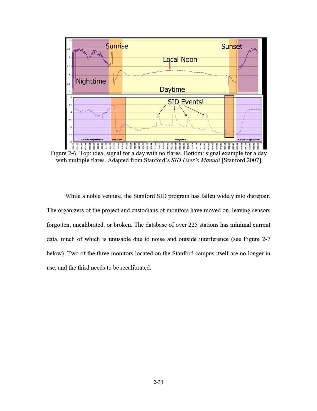
45 This project initially intended to use data from the Stanford University Solar Center solar center SID monitor network. During the International Heliophysical Year of 2007 and in partnership with the United Nations Bureau of Space Sciences, Stanford University s Solar Center and Electrical Engineering departments created a low cost SID monitor that was designed for distribution and use in all 193 countries around the world [Stanford 2007]. These monitors were designed to be built for under $100, used with any computer, and set up in a matter of hours. The design developed by Stanford was based on the receiver used by the American Association of Variable Star Observers (AAVSO), with modifications for easier set up and calibration. The Stanford program also established an online database for users to upload their data. Stanford provided instructions for building an inexpensive, efficient loop antenna consisting of square frame, 1 2 meters across, made from a non-conducting material wrapped times with an insulated wire. The SID monitor passes the raw signal through an amplifier, filters it by frequency, and converts it into a voltage signal. The signal strength is then plotted using software provided with the SID monitors. An ideal signal during a quiescent day will be stronger at night, variable during sunrise and sunset, and weaker during the day. The daytime signal is lowest after sunrise and before sunset and highest at local noon (see Figure 2-6 below). During a day with high solar activity, spikes of strong signal strength mark the occurrence of solar flares. 2-30

46

47 Figure 2-7. Plots from Stanford s SID database for 10 June Two different monitors looking at the same transmitter during two X-class solar flares. [Stanford 2014] Top: Example of a working monitor. Bottom: Example of a noisy, uncalibrated monitor. Fortunately, the AAVSO also maintains a collective database of SID occurrences dating back to The AAVSO database rates SIDs in intensity from -1 to +3, but no numerical data is provided on the details of signal enhancement. Numerical data is found, though, on some private websites running SID monitors. Two of the sites accessible via AAVSO s website became the foundation for data access for the remainder of this project. The first data source was SID monitor A131, run by Ján Karlovský of the Hlohovec Observatory in Slovakia, and the second was A118, privately run by Lionel Loudet, in Southern France. Information provided by Loudet includes detailed instructions for building both an antenna and a monitor, complete with schematics for how to design the circuit board. The antenna design is very similar to that of Stanford s loop design. Loudet s SID monitor filters the received VLF signal to the desired frequency, amplifies it, runs it through a bandpass filter to tune the signal, and converts it to a format readable by a computer (see Figure 2-8 below). Loudet also provides the necessary software and tools to calibrate the SID monitor and connect it to a Linux- or 2-32

48 Windows- based computer [Loudet 2013]. Whether privately-designed or mass-produced, the goal of the SID monitors remains the same, to allow interpretation of VLF signals. The wide access to publically available data from SID monitors around the world allows anyone to become an amateur astronomer or space weather scientist and allows professionals to collaborate with others across the globe. Figure 2-8. Block diagram of functions of a SID monitor. [Loudet 2013] 2-33

49 III. Methodology This chapter includes a discussion on the methodology used to collect and process the data from SID monitors and from the GOES-15 X-ray sensor. The first section will focus on the data collection and organization. Specifically, it will focus on the Stanford University Solar Center SID Program database and discuss why, as the primary data source presented with the project, it was discarded. Next, it will discuss the finding and acquisition of new data from both the Hlohovec Observatory and Loudet s site from Southern France. The second section includes discussion on the development of the MATLAB code used to process and analyze the data. 3.1 Data Collection GOES-15 XRS Data This study began with a proposal from the Air Force Research Laboratory, Space Vehicles Directorate, Kirtland Air Force Base, New Mexico. The first data provided, and the foundation for the project, was a list containing every M- and X-class solar flare recorded by the GOES-15 satellite from May 2010 through June This list comprised a total of 490 significant flare events. Each flare was listed with the date, UTC time, class, and magnitude (see Table 3-1 below). This list defined the search days for SID and GOES-15 data collection. GOES-15 XRS data were obtained via the NOAA website in.netcdf file format for each day in which there was an M- or X- class flare. The data was provided in two sets, long X-rays, 1-8 Å and short X-rays, Å (see Figure 3-1 below). 3-1

50

51 3.1.2 Stanford University Solar Center SID Monitor Data At the start of this project, in June 2014, the Stanford database contained data from 925 individual SID monitors. The monitors are divided among 225 operators in 38 countries spanning all seven continents, with some operators maintaining 20 monitors at once (see Appendix A). Each SID monitor analyzes one of 66 transmitters located around the world that each emit a steady LF or VLF radio signal ranging between 16.3 and 81 khz (see Appendix C). Organization of this expansive database was by far the most time consuming portion of the data collection process. Figure 3-2. Standford Solar Center SID Monitor [Stanford 2007] The Stanford database and user interface is well organized and easy to manipulate and understand. The default display, upon opening of the webpage, shows all of the monitors with data available for the current date displaying on a series of 24 hour graphs from 00:00:00 to 23:59:59 UTC. Each graph gives a plot of modified signal strength versus time labeled with the monitor name, numerical designation, and the transmitter 3-3

52 signal being recorded. There are options to change the duration of the graph from 1 day to 1 hour, 6 hours, or 3 days. Additional display options include vertical sunrise and sunset arrows for both the monitor location and the transmitter location, and times of any solar flares for that day as recorded by the GOES satellites. The solar flare options enable further grouping of flares, A through X, C and above, M and above, and X flares only. There are options available to search for data by date or by monitor in order to locate specific data. The monitor database allows the user to search by monitor name, station name, station location, or transmitter being monitored. Widespread network data is available from 2007, but there is also data available in the View Data by Date section from October 2005 to present for the two monitors on the Stanford campus. Most important, there is a link at the top of the page to Download Data Files. This link takes the user to a page with additional links to a series of.txt files. The page includes one link for every monitor selected for graphical display, and the numerical data used to make the plots. The files provided are listed by monitor name, transmitter being monitored, monitor numerical designation, date, and time. The text within the files contains header information about the station location, UTC offset, transmitter call sign, transmitter frequency, monitor identification number, and daily min and max values. The body of the data is provided in three columns at a five second sample rate containing date, time, and recorded signal strength. Data and plots are updated hourly to provide the most current information. The first step organizing the Stanford SID data was to consolidate from 925 individual monitors down to just the 225 stations. Of the 225 stations included in the online database, only 135 provided a country of origin. As research on SID phenomenon 3-4

53 commenced and study of the plots on Stanford s website continued, it became obvious that the monitor location and sunrise and sunset indicators were going to play a major role in filtering the useful data from the meaningless. As discussed in chapter two, SIDs are exclusively a daytime phenomenon. Therefore, in order for a SID to be detected, both the transmitter sending the signal and the monitor receiving it must be in daylight. With this knowledge, the next step in organizing the data became to determine precise monitor and transmitter locations. The Stanford Solar Center SID monitor home page includes a list of 41 of the most popular VLF transmitters across the globe. The spreadsheet contains the transmitter name and its frequency, city, country, latitude and longitude. Additionally the SID database contains a link to a Map of Monitors which contains an interactive Google Earth map marking the location of 338 SID monitors in 52 different countries (see Appendix B). The Google Earth markers provide city, country, latitude, longitude, site identification code, name of the school or organization hosting the site, and the monitor numerical designation. The first major problem arose when the map of monitors and the SID database did not match. Only 75 of the site identification codes, of the 225 from the database and 338 from the map, coincided. This fact diminished the number of potentially useful data sources by two-thirds. The next step in the organization process became determining the usefulness of the data available. This process began with selecting each station individually, then using the tool to View Data by Date. This course exposed the second major difficulty with the Stanford data source. While each monitor in the database had data available, some provided data for as few as four days out of the seven or more years the project was 3-5

54 running. Other monitors ran for a year or two before shutting down, which meant none of the data available coincided with the full GOES-15 satellite archive, effectively eliminating them as data sources for this project. Other monitors ran intermittently. Without a consistent SID dataset, the goal became to determine if any available data matched the list of flare occurrences provided by AFRL. The search began by looking specifically at X-class flares, limiting the number of flare occurrences from 490 to 34. Of the 75 monitors with known locations, only 27 recorded data during an X-class solar flare that was also reported by the GOES-15 satellite. Only one monitor in Germany provided data during all 34 X-class flares, while other monitors recorded less than 5. The final step was to determine the timing of the flare relative to the sunrise and sunset time of the monitors and transmitters recording the SIDs. In order for the signal to be intensified by a SID, the flare needs to occur when both the transmitter and the receiving SID monitor are in daylight. There was large distance between some Stanford SID monitor locations and the transmitting stations they monitored. For example, the monitor in Germany which recorded data during all 34 X-class flares, receives its signal from a transmitter in Cutler, Maine. The large distance between this monitor and transmitter allows, at best during the summer solstice, just under 10 hours where both locations are in sunlight. During the winter solstice, there is as little as two hours of shared daylight time between the two locations in which to potentially capture solar flare data. For this particular station, approximately half of the 34 flares occurred when both the monitor and transmitter were dark, as would be expected with diurnal changes in sunlight. Another ten X-class solar flares were lost due to only one location being in daylight. Overall, only four of the X-class flares were recorded when both the monitor 3-6

55 and transmitter were in daylight. The other sites proved similarly disappointing, and even X-class flares that were recorded were corrupted by noise and poor calibration. Stanford s SID monitor data proved unusable because the low price and mass distribution of monitors led to a lack of maintenance and calibration. A number of explanations could be given for individual monitor failures and signal degradation. Antennas could have been built with inadequate materials, or set up in locations with severe interference. They could also be subject to weathering. Monitors may never have been calibrated properly or lacked regular maintenance to ensure signal quality. Monitors given to universities and high schools were likely adopted by students one year and passed along to the next, or forgotten after a research project was finished. One such case was the Stanford SID monitor given to the United States Air Force Academy. The monitor was operated for two months as an independent study by a student in 2008 and When queried about the monitor in 2014, the student s department found it in a storage closet with the antenna in disrepair. While the database still exists, even the group that founded the project has moved on, leaving the website to run itself. During data collection for this study, the server for the database failed and was not restored for two weeks because the current project leader was unaware of the problem. Ultimately, the data from Stanford s Solar Center SID Monitor Database was abandoned due to minimal usable data and poor data quality AAVSO sites: Hlohovec Observatory and Southern France During the Stanford server outage, the search began for a new SID monitor and VLF data source. A website for the Hlohovec Observatory in Hlohovec, Slovakia was discovered and the data for its privately run SID monitor were discovered via the 3-7

56 AAVSO; its observer code is A131 (see Figure 3-3 below). The Hlohovec Observatory website is operated and its data maintained by Ján Karlovský, who proved extremely helpful for this project. The observatory s SID webpage contains multiple visual representations of SID and solar data: an hourly plots of three different transmitter signals versus time with the most recent data; a 24 hour plot of the same three transmitters on the current day; a 24 hour plot of 10 transmitters side by side along with a plot of background level noise; 6-hour GOES X-ray flux data; 3-day GOES X-ray flux data; 6-hour Solar Dynamics Observatory (SDO) Extreme Ultraviolet (EUV) Variability Experiment (EVE) data; 3-day SDO-EVE data; and the latest image from the SDO magnetogram [Kárlovský 2014]. The webpage also provides links for other monitoring stations and a series of educational links providing information on space weather and sudden ionospheric disturbances. The website also provides archives of overall monthly solar activity since The key to this project was in the link to the data center where the numerical data and basic plots for 2014 could be downloaded. 3-8

57 Figure 3-3. Google Earth image of SID monitors (green) and VLF transmitters (red). The Hlohovec website provided daily plots and raw numerical data from the DHO transmitter in northern Germany, at 23.4 khz, for all of The data was provided in.dat format aligned in two columns with time in seconds since midnight and signal strength in decibels. Data was sampled every 60 seconds from 0 to 86,280 seconds, or 00:00:00 to 23:59:00 UTC. Scrolling over the link to each file shows a visual preview of the graph the raw data will produce. The signal strength seen in the plots contained minimal noise, was received from a transmitter in the same time zone, and had data for every day of The site, however, was lacking any older data from previous years. The site author was contacted and he responded with data available for DHO from 2011 at a one-second resolution. In total, he sent 158 files containing all of the SID monitor data available corresponding to the days with solar flares. Finally, with a reliable and consistent source of data, data processing could begin. 3-9

58 While the Hlohovec Observatory offered a promising source of VLF signal data, it only provided data from one transmitter to one monitor. Another data source was desired for contrast, quality control, and ideally a comparison of how different frequency signals responded to the same flare event. The site in southern France, AAVSO code A118, run by Lionel Loudet, presented this second data source. This site provides radio signal data from one monitoring site that receives from nine different LF and VLF transmitters at various distances and frequencies, including the DHO transmitter observed by the Hlohovec Observatory. The monitoring site receives signals from GBZ (19.58 khz) in Great Britain, ICV (20.7 khz) in Italy, GQD (22.1 khz) in Great Britain, DHO (23.4 khz) in Germany, NAA (24.0 khz) in the United States, TBB (26.7 khz) in Turkey, NRK (37.5 khz) in Iceland, NSY (45.9 khz) in Italy, and DCF (77.5 khz) in Germany (see Figure 3-3 above). Loudet s website includes extensive narrative about SID events, the ionosphere, solar activity, radio signals, and details about the station and SID monitor. It also provides numerical and graphical data as far back as 2005 at tensecond resolution. An interactive graph provides GOES X-ray flux data and the ability to include any or all of the nine radio signals available. Downloadable files are provided in.txt format in a zipped folder containing all of the selected transmitters. Each.txt file contained three columns: a date, time (in hour, minute, second format), and signal strength. Loudet also provides a series of programs and base code using C to help analyze the data available and to interpret data from any new monitors developed using the schematics provided. The SunTimes program, which determines the sunrise and sunset times for a given location and date, proved particularly useful for helping to sort and analyze data. 3-10

59 3.2 Data Processing The data from both AAVSO sites comprised, 2,625 text files. Sorting through this massive amount of data and pinpointing exact times of solar flares in thousands of rows of text became the major challenge. Coding was done using MATLAB R2014b, and using Microsoft Excel as an intermediary to store spreadsheets of data for both input and output. The first goal in organizing the data was to combine AFRL flare data, GOES-15 X-ray data, and SID monitor data into one file, in order to present a side by side comparison of X-ray flux and VLF signal strength. The second major goal was to find a precise maximum value and time of occurrence for short and long X-ray flux and VLF signal strength. Coding began with the data from the Hlohovec Observatory as the use of only one transmitter simplified the process. To start, AFRL text data was tabulated into seven columns for the day, month, year, hour, minute, class, and magnitude for each solar flare. The spreadsheet was read into MATLAB. Variables were assigned to each column of data and empty columns were created to mark places for the incoming GOES and SID data. The new columns created held places for the peak short X-ray flux, the time of the peak short X-ray flux, the peak long X-ray flux, the time of the peak long X-ray flux, the time of maximum VLF signal strength, and the time of the maximum VLF signal strength. The final part of the program introduction established counters to run through a loop for every flare provided in the AFRL database. The first challenge presented was converting the tabular flare data into file names in order to match specific GOES and SID data files. The problem was single digits in the days and months were read in as single digits, and years as four digit number while the 3-11

60 file names for GOES and SID data were provided in yy/mm/dd format. In order to create file names, variables were created for the day, month, and year using the num2str command converting numbers from the table into text data. Then, to create double digit format from a single digit number, a series of if statements was used along with strcom to compare the date values to the numbers 1 through 9. If a single digit was encountered, the text value was changed to add a 0 in front of the digit, for example 1 is changed to 01. A similar process was used to drop the first two digits of the four digit year. With this accomplished, a full file name could be provided to MATLAB to look for a specific folder path and file name. The second challenge appeared when a date from the solar flare data did not exist in the Hlohovec Observatory folder. When this happened, the program ended in an infinite loop trying to pull data from files that did not exist. This required a simple fix of an added if statement to check if the filename existed. If the file existed, the program continued and opened the files. If not, it proceeded to the next flare by adding one to the loop counter and returning to the beginning of the program. The.netCDF format of the GOES-15 files was read by the intrinsic MATLAB command ncread, and the.dat format of the Hlohovec SID monitor data was read using the importdata command. The third data processing challenge came in the form of the different time formats. GOES data was provided in UNIX-epoch time, or number of seconds since 1 Jan 1970, Hlohovec data was provided in seconds since midnight, and French data was provided in hour, minute, second format. In order to convert the times into the same format, two separate scripts were written: converttime to work with the UNIX-epoch time, and converttime2 to work with the hour, minute, and second format. These two 3-12

61 programs converted the times into an hour decimal format that would be easy to plot in a 24 hour format. Once all the data was on the same timeline, the next step was to create the visual comparison by plotting the data. The first plot created was a 24 hour snapshot of short X-ray flux, long X-ray flux, and VLF signal strength (see Figure 3-4 below). The y-axis was plotted on a logarithmic scale to enhance the variance of the signal fluctuations. With X-ray flux increasing by as many as four orders of magnitude during a solar flare, much of the detail of the X-ray flux was lost on a linear scale while the sun was quiet. Next, using the AFRL flare data, the time and class of each flare was indicated with M-class flares marked with a vertical magenta lines, and X-class flares being designated by black lines. Figure 3-4. Example of a 24 hour plot from Hlohovec Observatory and GOES-15 hard X-ray flux (blue), soft X-ray flux (red), VLF modified signal strength (green), M class solar flares (magenta), X class solar flares (black). 3-13

62 The 24 hour plots allowed a direct comparison between signal strength and X-ray flux. The plot in Figure 3-4 was chosen as an example, not because it was ideal, but because it presented a variety of information. The plot contains both M- and X-class solar flares as well as a flare at night. It demonstrates the difference between the day and night signal strength, and that SID events are not recorded by VLF signals before sunrise or after sunset. Multiple C-class flares can be seen in the X-ray plots, however, these flares are not strong enough to significantly modify the ionosphere and no SID is observed with these events. It also demonstrates a loss of data around 0700 UT. This particular outage occurred when the transmitter stopped broadcasting, which was determined by the loss was observed by both the monitor in Slovakia and the monitor in France. Data from several SID events were lost when flares occurred during similar outages which lasted hours to days. Flares that occurred during near the day-night transitions were also lost in the signal fluctuations. All of this had to be considered in processing and analysis, to distinguish valid SID data from erroneous data recorded during these times. The fourth challenge came in determining if there was more than one flare on the same day. A while loop was created to determine if the next flare in the table had the same date as the flare before it. If so, another vertical line was added to the 24 hour plot to mark any subsequent flares. Once no more flares were found for the day, the 24 hour plot was complete, a new folder was created for the day, and the image saved. A counter was included in the while loop to track the number of extra flares for the day, which was then subtracted upon exiting the loop in order to return to the original flare being analyzed. This process enabled the second goal of finding a precise maximum value and time of occurrence for the X-ray flux and VLF signal strength for each flare. 3-14

63 The first step in accomplishing the second goal of finding a precise maximum value and time of occurrence for each the short and long X-ray flux and VLF signal strength, was to bracket the flare with a specific time window to block out any larger signals during the day, such as nocturnal returns or stronger flares. The bracket was set to 10 minutes before the flare to 50 minutes after in order to capture both the pre-flare and decay phases for the majority of flares. With the restricted timeline, a new plot was generated showing the 1 hour zoomed-in snapshot of each flare (see Figure 3-5 below). A new filename was created for each plot, and the figures were saved in the same folder as the 24 hour view. Figure 3-5. Example of a 1 hour zoom around a solar flare 3-15

64 The fifth challenge was finding the location of the start and end times in the data arrays. The first barrier in this challenge occurred with flares at either the start or end of the day where the 1-hour limit exceeded the 24 hour time line and a value did not exist in the GOES or SID array. This was overcome by logic recognizing when the pre-flare boundary was less than zero or the post-flare boundary was greater than 24, and resetting those boundaries accordingly. The second barrier arose with the start and end time arrays containing zero values. To find the start or end time, the desired time was subtracted from each value in the data array and then a search was conducted to find values differences smaller than the time step in seconds divided by 3600 seconds per hour. Most often, a zero value for the array would occur during a data drop-out where that time would not exist. To solve this, time was gradually subtracted at the start or added at the end in ten second intervals to increase the time bracket in order to find the edge of the data drop. A counter was included on this check, and if ten minutes in either direction was exceeded, it was assumed that the data drop was extensive enough to alter the data and the run was discarded, returning to the start of the program. If a value was found before the limits were reached, the start or end value was established and the run would continue. The next step in finding the maximum values was to use the starting and ending brackets for the array to narrow a search for the largest X-ray flux and VLF signal values and their time of occurrence. The maximum value was easiest to find using the max command to find the highest value within the bounds of the start and end values. The timing was more complicated. The first task was to find the position in the array where the maximum value occurred. 3-16

65 The final programming challenge arose when more than one value in the array held the maximum value. This most often occurred when the flare was at night and there was no peak value for the flare. When this occurred, a filter was applied to find the first location within the bounds of the start and end times. In order to find the time, the value contained in that spot of the array was recorded. After this was accomplished, the process of zooming in, plotting, and recording maximum values and times had to be repeated for each consecutive flare for the same date. This required proceeding to the next flare in the AFRL database without accessing new GOES or VLF signal data until all the flares for a single day were recorded. Once each day was completed, the next file with SID data was found along with the corresponding GOES data and the process was repeated. As the program runs, the arrays initialized in the beginning for maximum X-ray flux values, maximum SID values, and times of occurrence will be populated. At the completion of the program the six new column arrays are compiled into a single table and then combined with the existing flare data. Finally, the resulting table is exported to a spreadsheet for analysis. A second program was required to process the French data. This program was structured nearly the same as the program for the Slovakian data, but involved the additional loop structures needed to accommodate data from all nine transmitters for each flare. The other major addition to this program was the use of the SunTimes code provided by at Loudet s website [Loudet 2013]. This addition provided a major challenge since it was written in C. The purpose of the program was to find the sunrise and sunset time for given coordinates on specific days. This was necessary to filter the flares that occurred before sunrise or after sunset, to cut down on program run time and post 3-17

66 processing analysis. Minor alterations made to the original code included running it for multiple days instead of a single day and exporting the output to a spreadsheet. With almost 2,500 files from the French data site, limiting the selection by eliminating any flares that took place before sunrise or after sunset reduced program run time by almost two hours. This decreased the data load by approximately half. Folders were created for the data arranging each monitor specifically by date. 3-18

67 IV. Analysis and Conclusions 4.1 Hlohovec Analysis The post processed data contained the original AFRL flare data, with day, month, year, hour, minute, class and magnitude, combined with the SID monitor data from the Hlohovec observatory. The new data included a maximum short X-ray flux, time of the maximum short X-ray flux, maximum long X-ray flux, time of the maximum long X-ray flux, the maximum value of VLF signal strength, and the time of the maximum VLF signal strength (see Table 4-1 below). Table 4-1. Flare and VLF Signal Data Day Month Year Hour Min Class Mag MaxShort TimeShort MaxLong TimeLong MaxVLF TimeVLF VLF-Short X X E X E X E X 1 3.5E X M E E M E E The first step in analyzing the data was to eliminate the zeroes on the spreadsheet that occurred for days the observatory was not able to provide data. The next step was to eliminate any solar flares that occurred at night. This was done using NOAA s Solar Calculator [NOAA 2014]. The calculator provides the time of sunrise and sunset for a given latitude, longitude, and date. This process left 92 solar flares of the 278 flares that occurred on days for which Hlohovec provided data. Additional filtering eliminated flares occurring just after sunrise or just before sunset that were lost in the signal fluctuations along these boundaries. Additionally, SIDs that occurred during times when the DHO 4-1

68 transmitter was not broadcasting or other data loss occurred were considered anomalous and disregarded. To aid the elimination process, a plot was created comparing the time of maximum X-ray flux to maximum VLF signal strength (see Figure 4-1a below). This plot allowed visualization of anomalous data points, making it easy to pinpoint the raw data and the 24 hour plot associated with that data in order to isolate and eliminate the problem data from the analysis. Once the zeros, pre-sunrise and post-sunset, and dropout data were eliminated, 63 flares remained (see figure 4-1b below). a. b. Figure 4-1. a. Unfiltered data from Hlohovec Observatory b. Data from Hlohovec Observatory with zeros, pre-sunrise, post-sunset, and anomalous data removed 4-2

69 The remaining 63 flares were then analyzed by plotting maximum VLF signal strength as a function of flare magnitude (see Figure 4-2 below). The flare magnitude was modified to fit the logarithmic classification. M1.0 through M9.9 flares were designated 1 through 9.9 along the x-axis, and each X-class magnitude was multiplied by 10, making X1.0 equivalent to 10 along the x-axis. A second filtration was made after realizing that the first 13 flares recorded by the monitor, colored in orange in Figure 4-2, appeared anomalous when compared to the rest of the data. The signal responses from these flares were an average of decibels stronger than other flares of similar magnitudes. These 13 flares occurred in February and March of 2011, followed by a five month period where no data was available. It is likely that maintenance or recalibration occurred during that time period. The Hlohovec data was then separated and each set plotted individually and a linear regression analysis completed (see Figure 4-3 below). Figure 4-2. VLF signal strength as a function of solar flare magnitude as recorded by Hlohovec Observatory 4-3

70

71 4.2 Southern France Analysis The data from Southern France was processed in a similar manner. The SunTimes program was used to filter out flares occurring before sunrise and after sunset rather than the hands on method used in analyzing the Hlohovec data. It proved necessary to analyze each transmitter separately as each transmitter displayed different outages and days without available data. Unlike the Hlohovec data which did not provide data on days the monitor or transmitter were down and those files were recorded as zeros, the Southern France site had data for every day whether the transmitter was running or not. This, and the addition of 8 transmitters to the data set, greatly increased the time required for analysis of these files. After filtering the data by eliminating pre-sunrise, post-sunset and data dropouts for each transmitter, plots were made to compare the maximum VLF signal response to the flare magnitude, as was done with the data from the Hlohovec Observatory. The French data, however, showed surprising results, in that there was no correlation between the strength of the flare and signal response recorded by the SID monitor (see Figure 4-4 below). The DHO transmitter was chosen to show a direct comparison between the Hlohovec Observatory data and the Southern France data, however, the other 8 transmitters displayed a similar lack of correlation. Further analysis of the DHO signal plots created in MATLAB verified this lack of correlation between maximum VLF signal strength and solar flare magnitude (see Figure 4-5 below). In Figure 4-5 a side-by-side comparison of the Hlohovec plot and the Southern France plot for the same transmitter can be made. The figure shows plots for an M3.0 flare and an X1.0 flare which occurred 4-5

72 57 minutes apart. In the Hlohovec plot, a clear difference in signal responses can be seen, while in the Southern France plot the strength of the responses are nearly identical. Figure 4-4. DHO signal strength as a function of solar flare magnitude as recorded by Lionel Loudet October 2010 June

73 Figure 4-5. Comparison of DHO VLF signal response between Hlohovec Observatroy and Southern France. With this surprising discovery, a second theory was postulated considering the possibility of diurnal or seasonal variations. The French data proved ideal for this hypothesis, showing clear seasonal variation (see Figure 4-6 below). Data was divided by season defining the winter months as January, February, and March, the spring months as April, May, and June, the summer months as July, August, and September, and the autumn months as October, November, and December. Days along the x-axis were determine by what day of the year, out of 365 days, a flare occurred. No consideration was given in this analysis as to which year the flare occurred in. The trend lines in this plot were completed using a 5 th order polynomial expansion. Additionally, in this plot there is a clear difference in signal response with respect to the frequency. GBZ, 19.6 khz, had the lowest frequency and the highest signal response through all four seasons, while DCF, 77.5 khz, showed the lowest response. The NAA, 24.4 khz, and NRK, 37.5 khz, trend lines consecutively decrease between the GBZ and DCF trend lines showing a 4-7

74 pattern that higher frequency waves show decreased influence by corresponding SID events. Figure 4-6. Variation of signal strength by season. Seasons delineated by the color of the background; Winter (blue) Spring (green) Summer (yellow) and Fall (red) 4.3 Conclusions Research objectives for this project included the creation of a database for LF and VLF SID events corresponding to solar flare occurrence and X-ray flux, the measurement of ionospheric incubation time between peak X-ray flux and peak SID response, the analysis of how different radio frequencies respond to the same SID event, the analysis of how maximum X-ray flux correlates to LF and VLF signals in the atmosphere, the search for seasonal or diurnal variation in SID response, and the relation of SID rise time, 4-8

75 duration and decay time compared to X-ray flux measurements. The creation of a database began with looking at Stanford s Solar Center s SID Monitor program, and while this did not prove a useful source of data, many lessons were learned about SID dynamics and observation. The most important of these lessons was that both monitor and transmitter must be in daylight to successfully observe a SID as the discontinuity at the day-night terminator disrupts the signal propagation. With this knowledge in mind, two new SID monitoring sites were chosen: Hlohovec Observatory in Hlohovec Slovakia, and a privately run monitor in Southern France. The DHO transmitter observed by both sites provided quality control and a direct comparison between the operations of the different monitors. Between the two sites and the nine transmission frequencies, data was collected for over 4500 observed solar flare events. This data was processed into a series of 24-hour and 1-hour plots directly comparing the LF or VLF signal strength with the X- ray flux values recorded by the GOES-15 satellite. The ionospheric incubation times were calculated using the analysis done to find times for peak values of both X-ray flux and modified LF or VLF signal strength. The time of the maximum recorded signal strength for each transmitter was subtracted from the time for the peak X-ray flux. It was found, across all the transmitters, the ionospheric incubation time averaged 2.7 minutes. The largest average incubation time was observed by the DCF transmitter at 3.4 minutes with the shortest observed by GBZ at 2.1 minutes. Further analysis needs to be done to determine if there is a correlation between solar flare magnitude and ionospheric incubation times. The Southern France SID monitoring site allowed for a comparison of how different frequencies respond to the same SID events. The general trend between October 4-9

76 2011 and June 2014 showed that lower frequencies show the greatest enhancement of signal during SID events. There is a crossover of signal strength seen in Figure 4-6 during the later portion of the winter months which could be an error introduced by the polynomial best fit function or a consequence of all the signals being at a minimum making them nearly indistinguishable on the scale provided. Overall, the difference in signal response is logical as the D-region is the reflector of VLF frequencies. The higher frequencies in the LF range, penetrate further into the D-region and will experience greater attenuation over the extended path length. When starting this research it was hypothesized that the SID modified VLF signal strength would directly relate to the increase of X-ray flux. The amount of X-ray radiation received at Earth should directly correlate to the amount of photoionization in the ionosphere creating higher electron densities in the D-region. The enhanced TEC in the D-region increases its conductivity and the reflection of the radio waves occurs at lower altitudes without experiencing as much atmospheric attenuation. This phenomenon was clearly expressed by the data acquired from the Hlohovec Observatory showing a linear correlation between received signal strength and flare magnitude. It is well known that the ionosphere varies with diurnally and seasonally depending on the amount of direct sunlight received at the top of the atmosphere. The height of the ionosphere is lower in summer and during the day and electron densities are higher. With this, it was expected that SID strength might also vary by season. This was clearly seen in the Southern France data where the enhancement of LF and VLF signal strength in the summer was approximately double that seen in the winter months. 4-10

77 While time constraints did not allow for a quantitative analysis of SID rise, duration, and decay times, a qualitative analysis was accomplished using the plots created in MATLAB. Visualization of LF and VLF signal enhancement displayed alongside X- ray flux enhancements displayed a coincident pattern in the rise and duration times of the two events. Decay times of signal enhancement however, were much greater than that of the X-ray flux. This is due to the recombination rate of ions in the D-region being slower than the photoionization rate which created the SID event. 4.4 Future Work While the research objectives for this project were met, there is still extensive work which could be done to further the understanding and usefulness of the data. In expanding the research objectives, the most obvious desire would be for additional data and expansion of the database created during this project. There are many AAVSO sites that were not used in this research that could be exploited for further comparison and a deeper understanding into the drastically different results between the Hlohovec Observatory and Southern France monitoring stations. The ionospheric incubation times were calculated at face value, and could be further analyzed to determine if there is a correlation with flare magnitude or seasonal variation. While seasonal variations were approached in this research, diurnal variations were not taken into account, as there was not enough flares of comparable magnitude spaced close in time. When this project was proposed, a quantitative analysis was desired looking for precise rise, duration and decay times. This could be accomplished by using a baseline integration comparing signal enhancement on a day with SID events to a day with no SID events. 4-11

78 Beyond the initial research objectives, additional work could include expanding the research to analyze different types of SID events other than the SES analyzed here. This could be accomplished by using data from the Atmospheric Weather Electromagnetic System for Observation, Modeling, and Education (AWESOME) monitors developed by Stanford which analyze signal phase and amplitude side-by-side. Additionally, higher frequency waves could be analyzed and the responses of the E and F regions to X-ray and EUV enhancements. Additionally, the creation of a computational model to investigate propagation paths by altering characteristics of the Earth-ionosphere waveguide could be useful in predicting more precise effects on radio transmissions. 4-12

79 Appendix A: Stanford Solar Center Online Database Station ID Monitors at Station Station Location Firat University Arts & Science, Elazig, Turkey S. Webster, OH, USA USA Sula, Montana, USA Wheelersburg, OH, USA Mexico USA Antarctica Vienna, Austria USA Malaysia USA Slovenia USA Sweden USA A-1

80 Appendix A: Stanford Solar Center Online Database Station ID Monitors at Station Station Location Baku, Azerbaijan Lagos, Nigeria Canada Canada Italy USA USA Brazil McDonough School, Reisterstown, Maryland, USA USA Crotia Greece UK Tunisia Vietnam USA Canada A-2

81 Appendix A: Stanford Solar Center Online Database Station ID Monitors at Station Station Location Canada USA USA USA USA Brazil College of Staten Island, Staten Island, NY, USA USA India Brazil India A-3

82 Appendix A: Stanford Solar Center Online Database Station ID Monitors at Station Station Location Dordogne-Perigord, France Nigeria Colegio Santa Maria De Santiago, Santiago, Chile Konstanz, Germany USA McMath-Hulbert Solar Observatory, Lake Angelus, Michigan, USA Grants Pass, Oregon, USA USA Uruguay Australia USA USA USA Venezuela Venezuela Sweden Canada Tunisia France USA A-4

83 Appendix A: Stanford Solar Center Online Database Station ID Monitors at Station Station Location USA USA UK AAVSO-1 1 Cambridge, Mass, USA AAVSO-2 1 USA Astronomy 4 Eagan, MN DARO01 6 ERAC001 8 JASPER 5 N2YO 6 Chantilly, VA, USA New-SuperSID China New-SuperSID Petroleum Middle School, Daqing, China NONE 4 P003 7 USA Ref 1 Wilcox Solar Observatory, Stanford, California, USA S-0000-FB S-0000-FB India S Chabot Space & Science Center, Oakland, California, USA S Wilcox Solar Observatory, Stanford, California, USA S USA S0018-FB USA A-5

84 Appendix A: Stanford Solar Center Online Database Station ID Monitors at Station Station Location S-0021-FB South Side HS, Commack HS, Manhattan, NY, USA S-0022-FB USA S-0023-FB Utah State University, Logan, Utah, USA S-0025-FB West Valley High School, Fairbanks, Alaska, USA S USA S-0026-FB George Observatory, Richmond, TX, USA S Neustrelitz, Germany S-0029-FB Southwestern University, Gerogetown, TX, USA S-0031-FB Amsterdam, Netherlands S Brazil S-0036-FB Ponta Grossa State University, Parana, Brazil S Maharashtra, India S-0039-FB S Alabama A&M, Normal, Alabama, USA S-0042-FB Harvard-Smithsonian, Cambridge, Maryland, USA S-0045-FB Rice University, Houston, TX, USA s-0048-fb Hopkinsville Community College, Hopkinsville, KY, USA S-0049-FB USA S Anderson High School, Cincinnati, OH, USA S-0054-FB Suffolk County Community College, Selden, NY, USA S Dublin, Ireland S University of Porto, Porto, Portugal S Herfordshire, GB S North Carolina A&T State University, N. Carolina, USA S-0070-FB German Aerospace Center, Neustrelitz, Germany S CIRES/EVE, Boulder, Colorado, USA A-6

85 Appendix A: Stanford Solar Center Online Database Station ID Monitors at Station Station Location S-0077-FB USA S Gymnasium Walsrode, Walsrode, Germany S Felix Klein Gymnasium, Goettingen, Germany S-0087-FB Ernst Moritz Arndt Gymnasium, Bergen, Germany S-0088-FB Johannesburg, South Africa S-0090-FB Hamilton Amateur Astronomers, Ancaster, Ontario, Canada S Instituto Geofisico Universidad Javeriana, Bogota, Columbia S-0096-FB University of Tunis El Manar I, Tunis, Tunisia S-0099-FB Texas Lutheran University, Sequin, TX, USA S Inter-University Centre for Astronomy & Astrophysics, Pune, India S-0207-FB Uruguay S Auckland University of Technology, New Zealand S Iganmode Grammar School, Ota, Nigeria S-0220-FB Universidad Nacional Autonoma de Mexico, Monterrey, Mexico S-0224-FB Blue Ridge Learning Center, Todd, N. Carolina, USA S-0232-FB USA S-0232-FB Karns HS, Karns, TN, USA S-0239-FB Tunisia S-0240-FB Mexico S-0249-FB Nigeria S-0256-FB Center for Radio Astronomy, Belgrade, Serbia S Puebelo, Colorado, USA S-0258-FB USA S-0258-FB USA S-0261-FB Osservatorio Astronomico di Torino, Torino, Italy S-0263-FB Archenhold Sternwarte, Berlin, Germany A-7

86 Appendix A: Stanford Solar Center Online Database Station ID Monitors at Station Station Location S-0272-FB Nigeria S University of Congo, Kinshasa, Congo S Sebha University, Sebha, Libya S-0293-FB Nigeria S-0405-FB Liceo Classico C. Alberto, Novara, Italy S-0408-FB Liceo Valdese, Torre Pellice, Italy S Nigeria S-0420-FB Italy Schools, Rome, Italy S-0423-FB Italy Schools, Rome, Italy S-0426-FB Italy Schools, Rome, Italy S-0811-FB Austria S Denmark S-0816-FB USA S Brazil S Ankorage, AK, USA S-0821-FB Korea S-0823-FB China S China S-08280FB China S Germany S-0847-FB Canada S-0849-FB USA S-0850-FB USA S-1003-FB Uganda S-1013-FB Asociatia Astroclubul Bucresti, Bucharest, Romania S Astronomical Observatory, Astronomical Association of Zagreb, Zagreb, Croatia A-8

87 Appendix A: Stanford Solar Center Online Database Station ID Monitors at Station Station Location S Foods Technology College, Ulaanbaatar, Mongolia S-1032-FB Clarence Jones Observatory, University of Tennessee at Chattanooga, Hixson, TN, USA S-1035-FB St Johnsbury Academy, St Jonhsbury, Vermont, USA S Nomuun School, Ulaanbaatar, Mongolia S-1056-FB Korea Science Academy, Busan, Republic of Korea S USA SARA-SS 4 USA SJF SuperSID_ SuperSID USA SUPERSID India SuperSID China SuperSID Floral Park, NY, USA SuperSID-BCHS 21 China TinySID Netherlands UKM_SID37 6 Malaysia WSO-SS 6 USA Listed in Online Database Listed on Map as SuperSID Listed on Map as having data available in Online Database Listed on Map as not having data available in Online Database A-9

88

89

90

91

92

93

94

95

96