Modeling, Implementation, and Simulation of Two- Winding Plate Inductor

Transcription

1 Modeling, Implementation, and Simulation of Two- Winding Plate Inductor Han Cui Dissertation submitted to the faculty of the Virginia Polytechnic Institute and State University in partial fulfillment of the requirements for the degree of Doctor of Philosophy in Electrical Engineering Khai D. T. Ngo (Chair) Guo-Quan Lu Louis Guido Qiang Li Dong S. Ha April 28 th, 2017 Blacksburg, Virginia Keywords: magnetic field, plate-core, planar magnetics, inductance Copyright 2017, Han Cui

2 Modeling, Implementation, and Simulation of Two- Winding Plate Inductor Han Cui Abstract Design of magnetic component is a key factor in achieving high frequency, high powerdensity converters. Planar magnetics are widely used in bias power supplies for the benefits of low profile and their compatibility with printed-circuit boards (PCB). The two-winding inductors with winding layers sandwiched between two core plates are studied in this dissertation in order to model the self-inductance, winding loss, and core loss. The most challenging task for the plate-core inductor is to model the magnetic field with finite core dimensions, very non-uniform flux pattern, and large fringing flux. The winding is placed near the edge of the core to maximize the energy within the limited footprint where the amount of energy stored outside the core volume is not negligible. The proportional-reluctance, equal-flux (PREF) model is developed to build the contours with equal amount of flux by governing the reluctance of the flux path. The shapes of the flux lines are modeled by different functions that guided by the finite-element simulation (FES). The field from the flux lines enables calculation of inductance, winding loss, and core loss, etc.

3 The inductance matrix including self-inductance and mutual inductance of a two-winding inductor is important for circuit simulation and evaluation. The derivation of the inductance matrix of inductors with plate-core structure is described in Chapter 3. Two conditions are defined as common-mode (CM) field and differential-mode (DM) field in order to compute the matrix parameters. The proportional-reluctance, equal-flux (PREF) model introduced is employed to find the CM field distribution, and the DM field distribution is found from functions analogous to that of a solenoid s field. The inductance calculated are verified by flex-circuit prototypes with four different air gap lengths, inner winding radius, and number of turns. The application of the inductance model is presented at the last with normalized parameters to cover structures within a wide-range. In circuit where two-winding inductors are used instead of transformers, the phase shift between the primary and secondary side is not always 180 degrees. Therefore, it is important to model the winding loss for a two-winding inductor accurately. The winding loss can be calculated from the resistance matrix, which is independent of excitations and only relates to the frequency and geometry. The methodology to derive the resistance matrix from winding losses of twowinding inductors is discussed. Winding loss model with 2D magnetic field is improved by including the additional eddy current loss for better accuracy for the plate-core structures. The resistance matrix calculated from the model is verified by both measurement results and finiteelement simulation (FES) of two-winding inductor prototypes. Accurate core loss model is required for designing magnetic components in power converters. Most existing core loss models are based on frequency domain calculation, and they cannot be implemented in SPICE simulations. The core loss model in the time domain is discussed in Chapter 5 for arbitrary current excitations. An effective ac flux density is derived to simplify the core loss

4 calculation with non-uniform field distribution. A sub-circuit for core loss simulation is established in LTSPICE that is capable of being integrated to the power stage simulation. Transient behavior and accurate simulation results from the LTSPICE matches very well with the FES results. An equivalent circuit for coupled windings is developed for inductors with significant fringing effect. The equivalent circuit is derived from a physical model that captures the flux paths by having a leakage inductor and two mutual inductors on the primary and secondary side. A mutual resistor is added to each side in parallel with one mutual inductor to model the winding loss with open circuit and phase-shift impact. Two time-varying resistors are employed to represent the core loss in the time-domain. The equivalent circuit is verified by both finite-element simulation (FES) and prototypes fabricated with flexible circuit.

5 Modeling, Implementation, and Simulation of Two- Winding Plate Inductor Han Cui General Audience Abstract Compact power supplies requires low profile, high quality magnetic components such as inductors and two-winding inductors in order to achieve high efficiency and high density. The plate-core inductors comprise multilayer windings sandwiched by two core plates on the top and bottom, and the total thickness of the inductor is significantly smaller than the conventional surface-mount inductors. A model based on physical examination of the flux pattern is developed to calculate the magnetic field distribution of the plate-core inductor. The other performance factors such as inductance, winding loss, and core loss can also be calculated from the field distribution. An improved equivalent circuit is developed in order to simulate the voltage and current of the inductor in an arbitrary circuit. Compared to conventional equivalent circuit, the improved model includes the winding-loss variation with asymmetric current excitations. A coreloss sub-circuit is developed in SPICE simulation tools so that no finite-element simulations (FES) are required to obtain the core loss in the time domain, and the cost of time is reduced by more than 80%. A prototype is fabricated with inductors of different geometrical dimensions to verify the equivalent circuit under small signal condition. Good correlations among calculation, FES, and measurement are obtained with less than 13% error.

6 Acknowledgments I give my gratitude to my parents Yajing Han and Zhenduo Cui, and my husband Lingxiao Xue, who have always been supportive and understanding during these years. I could never reach this stage without their love. I am also grateful to my co-advisor, Dr. GQ. Lu, who shares a great amount of knowledge, suggestions, and experience with me. I appreciate his generous help and encouragement, which inspire me a great deal and raise my self-confidence. Sincere thanks to my other committee members, Dr. Qiang Li, Dr. Louis Guido, and Dr. Dong Ha, for their valuable suggestions and comments on my work. It has been a great pleasure to work with my talented colleagues at CPES. It is not possible to list all the names here, but thanks to all the people who helped me during the past six years. I appreciated and enjoyed the working and learning experience. Finally, I would like to give my deepest gratitude to my advisor, Dr. Khai Ngo, for his advising, encouragement, and patience. I am fortunate to have him as my advisor for my graduate study, or even my life. It is his extensive knowledge, his rigorous attitude towards research, and his scientific thinking to solve problems that enlightens me as to what makes a superior researcher. Without his generous help, it would be impossible for me to overcome so many difficulties and complete my PhD research. Thanks to Texas Instruments for funding this research. vi

7 Table of Contents Chapter 1 Introduction... 1 Nomenclature Isolated Bias Power Supply for Telecom Applications Two-winding Inductors in Bias Power Supply Benefits and Challenges of Plate-Core Inductors Existing Methods for Modeling Field of the Plate-Core Inductor Hurley s Method Current-Image Method Transmission-Line Method Conventional Equivalent Circuit for Two-Winding Inductors T-Model Isolated Model Contributions of This Dissertation Magnetic Field Modeling for Plate-core inductors with Finite Core Dimension Self-Inductance Model with Wide Range of Application Winding Loss Model with Non-Uniform 2D Field Distribution SPICE Simulation Circuit for Transient Core Loss Improved Equivalent Circuit for Coupled Windings vii

8 1.5 Dissertation Outline Chapter 2 Proportional-Reluctance, Equal-Flux Model for Magnetic Field Nomenclature Introduction Plate-Core Inductor Methodology Functions for the Flux Lines Fringing Region Core Region Winding Region Reluctance Calculation Reluctance in the Winding Region Reluctance in the Core Region Reluctance in the Fringing Region Modeling Results Complete Flux Lines Modeling Results of the Magnetic Field Implementation Summary Chapter 3 Inductance Modeling viii

9 Nomenclature Introduction Inductance Matrix Calculation Common-mode (CM) Field Modeling Differential-mode (DM) Field Modeling Simplified Structure without Spacing Methodology Experimental Verification Exemplary Utilization of Model Implementation Summary Chapter 4 Winding Loss Modeling Nomenclature Introduction Resistance Matrix of Two-winding Inductor D Magnetic Field around Winding Turns Conventional Models for 2D Winding Loss Winding Loss Calculation with Additional Eddy Current Loss Additional Eddy Effect in the Windings Normalized Function for Eddy Current Loss ix

10 4.3 Valid Range of Improved Winding Loss Model Experimental Results Exemplary Utilization of Model Implementation Summary Chapter 5 Time-Domain Core Loss Modeling Nomenclature Introduction Review of Core Loss Models Dynamic Core Loss Model for Ferrite Wipe-out Rule for Bm Extraction of Core Loss Parameters Steinmetz Parameters Effective Field Factor for Non-uniform Field Sub-Circuit Modeling for Dynamic Core Loss in LTSPICE Functions of Each Block in Core Loss Sub-Circuit Simulation Results of an Example Exemplary Utilization of Model Analytical Equation of Δ for Toroidal Structure Values of Field Factor Δ for Plate-Core Structure x

11 5.4.3 Steinmetz Parameters for Commercial Materials Summary Chapter 6 Improved Equivalent Circuit for Coupled Windings Nomenclature Introduction Open-Circuit Winding Loss Impact of Phase-Shift on Winding Loss Dynamic Core Loss Equivalent Circuit from Flux Distribution Flux Distribution Reluctance Network Circuit Network Parameter Extraction Inductances and Winding Loss Resistances Core Loss Resistors Exemplary Equivalent Circuit of a 2:1 Two-winding Inductor Simulation Results Open-Circuit Winding Loss Impact of Phase-Shift on Winding Loss Dynamic Core Loss xi

12 6.5 Exemplary Utilization of Model Implementation Summary Chapter 7 Conclusions and Future Work Summary of Work Future Work References 174 Appendix A Appendix B Appendix C Appendix D Appendix E Appendix F xii

13 List of Figures Figure 1.1. Isolated dc-dc power module in 1/8th brick from Texas Instruments [162] (a) top side and (b) bottom side Figure 1.2. (a) Synchronous buck converter topology with single inductor; (b) isolated buck converter (fly-buck) topology with two-winding inductor [3] for bias power supply Figure 1.3. LTM8058 µmodule converter from Linear Technology with mm 3 package size, V output voltage, and 1.5 W output power [5]... 3 Figure 1.4. LPD 5030V series miniature high-isolation 1:1 two-winding inductor with 1500 V isolation voltage at least occupy 5 5 mm 2 footprint and 2.9 mm thickness for an inductance of 4.7 µh [6] Figure 1.5. (a) Planar sandwich structure with 5 5 mm 2 footprint, total thickness less than 1 mm, and 3.5 µh inductance; (b) axisymmetric view of the cross section of the plate-core inductor in (a) showing the flux density distribution and flux direction Figure 1.6. Conventional inductor structure with toroidal core and square core showing relatively uniform flux density, effective area, and effective length for inductance calculation in (1.1) Figure 1.7. Energy density distribution across the cross-sectional area of the plate-core inductor (Figure 1.5(a)) with 1 A current excitation showing the center-air region, core, fringing, and the zero-flux position Figure 1.8. (a) Exemplary plate-core structure with winding widow width (R wo R wi = 0.7 mm) and (b) the energy percentage in the winding region, core region, and fringing region by sweeping the location of winding window R wo with fixed window width Figure 1.9. (a) Simulated inductance and (b) the product of inductance and dc quality factor versus R wo for the platecore inductor in Figure 1.8(a) by sweeping R wo position (keep R wo R wi = 0.7 mm) Figure Comparison of inductance simulated and calculated from Hurley s method versus core radius R c normalized to the outer winding radius R wo for structure shown in Figure 1.9(a) Figure Concept drawing of current-image method by reflecting the current to the top core and bottom core alternatively Figure Comparison of inductance simulated and calculated from current image method versus normalized core radius (R c/r wo) and normalized core thickness (H c/l g) for structure shown in Figure 1.9(a) xiii

14 Figure Cross section of a thin film head showing a line integral enclosing a current Figure T-model of a two-winding inductor Figure Isolated equivalent-circuit of a two-winding inductor Figure Modeled flux lines from PREF model to calculate non-uniform magnetic field distribution Figure Comparison of winding loss calculated from improved model with simulation and conventional model in [82] after considering additional eddy current loss caused by penetrating flux Figure Dynamic core loss with arbitrary current simulated in LTSPICE and FES Figure Improved equivalent circuit for two-winding inductors considering impact of open-circuit and phase shift on winding loss with time-varying core loss resistors Figure Outline and contributions of the dissertation Figure 2.1. (a) Plate-core inductor; (b) 2D cross-section view in cylindrical coordinates showing equal-flux contours and constituent reluctances of one path Figure 2.2. The flux density of an arbitrary point sandwiched by two equal-flux contours Figure 2.3. Shape of flux lines at the cross-sectional area and initialized path for calculation of total reluctance Rpath_1 and magnetic flux Φ shown in Figure Figure 2.4. (a) Plate-core inductor with fringing flux lines in the physical domain; (b) structure in the strip domain with infinite large core and straight flux lines Figure 2.5. Simulated and modeled θ f along the right edge of the core plate from 0 to H c in Figure 2.3 for Z p < z < Z p + H c at r = R c Figure 2.6. Simulated and modeled θ p in Figure 2.3 versus radius Figure 2.7. Reluctance calculation in the fringing region between i th and (i+1) th contours showing the cross-sectional areas and incremental magnetic length Figure 2.8. Flow chart to obtain the complete flux lines for plate-core inductors Figure 2.9. Plot of flux carried by one path versus the total number of paths for structure with dimensions in Table 2.1 and 1 A current excitation Figure Comparison of (a) simulated flux lines and (b) flux lines constructed based on proportional reluctance, equal-flux model under same scale for the plate-core inductor with dimensions listed in Table xiv

15 Figure Comparison of magnetic flux density along the path shown in Figure 2.10 (a) in the winding region; (b) in the core region; (c) in the fringing region Figure Comparison of energy breakdown between (a) simulation and (b) PREF model for the plate-core inductor with dimensions listed in Table Figure 3.1. Definition of (a) common-mode condition and (b) differential-mode condition Figure 3.2. Impact of number of layers on the total energy with 16 A Ampere-turns and other geometrical dimensions listed in Table Figure 3.3. Impact of vertical distance S ps between the winding layers on the total energy with other geometrical dimensions listed in Table Figure 3.4. Comparison of flux lines between (a) single-winding inductor and (b) two-winding inductor with dimensions listed in Table Figure 3.5. Inductance calculated from (3.6) versus (a) core radius, (b) gap thickness, (c) number of turns, (d) relative permeability, and (e) winding width. Dimensional parameters are normalized to the core radius R c. When a variable is being swept, the other parameters are kept at the nominal conditions as shown in Table Figure 3.6. Comparison of magnetic field distribution H mag between (a) original plate-core structure with 16 turns on each layer, and (b) simplified no-spacing structure with dimensions in Table Figure 3.7. Comparison of leakage inductance between original plate-core structure and the corresponding simplified structure with no spacing as shown in Figure 3.6, parametric with (a) inner winding radius, (b) spacing between winding turns, (c) spacing between primary and secondary windings, (d) material permeability, (e) core thickness, (f) winding height, and (g) number of winding turns Figure 3.8. Parameters used for calculating radial field component H r along radial line rr Figure 3.9. Parameters used for calculating vertical field component H z along radial line rr and vertical line zz Figure (a) H r field along r-direction, (b) H r field along z-direction, (c) H z field along r-direction, and (d) H z field along z-direction for simplified structure with no spacing with dimensions listed in Table 3.1 and parameters labeled in Figure Figure Comparison of (a) simulated magnetic field H mag in FES and (b) modeled magnetic field H mag under DM condition with dimensions listed in Table xv

16 Figure Modeled DM inductance calculated from (3.12) using simplified structure without spacing versus (a) inner winding radius, (b) spacing between primary and secondary windings, (c) winding height, (d) air gap length, and (e) permeability compared to FES with original 16-turn structure. The other parameters are kept at the nominal conditions as shown in Table 3.1 when one parameter is varied Figure Layouts of winding matrix fabricated with flexible circuit for inductance verification Figure Prototype of one inductor layout (a) top view and (b) side view Figure Assembly process of two-winding inductor prototype using two layers of flexible circuits and ferrite core material Figure (a) Customized four-terminal testing fixture and (b) an exemplary layout of the inductor on the flexible circuit Figure Testing setup of inductor prototype using customized testing fixture and Impedance Analyzer [168] Figure Comparisons of measured open-inductance with FES and modeled results under different (a) air gap length, (b) winding inner radius, and (c) number of turns Figure Comparisons of measured short-inductance with FES and modeled results under different (a) air gap length, (b) winding inner radius, and (c) number of turns Figure (a) Plate-core structure used for inductance synthesis and (b) nominal inductance (L/N 2 ) versus number of turns with R wi = 0.9 mm and R wo = 1.65 mm for the structure in Table Figure Relationship between the normalized inductance and the normalized inner winding radius parametric with normalized (a) core thickness, (b) air gap length, and (c) relative permeability with the parameters in Table Figure 4.1. Example structure of plate-core inductor with single winding Figure 4.2. Simulated 2D field (a) H x magnitude, (b) H y magnitude, (c) H x vector, and (d) H y vector for structure shown in Figure Figure 4.3. Closed-core structure used for conventional 2D winding loss model with parallel flux to the surfaces Figure 4.4. Comparison of simulated total winding loss and calculated loss using (4.13) - (4.17) for the structure shown in Figure 4.1 with variable winding width under 1 A current excitation at 5 MHz xvi

17 Figure 4.5. Comparison of (a) simulated winding loss and calculated loss in the first turn for the structure shown in Figure 4.1 with 80 µm winding width, (b) winding loss in the first turn versus normalized winding width to skin depth between simulation and calculation Figure 4.6. Flux around the winding turns of plate-core inductor showing vertical flux penetrating the winding surfaces Figure 4.7. The non-uniform magnetic field H y distribution along x-direction across the windings in Figure 4.1 with 1A current under 0 to 10 MHz frequencies Figure 4.8. Curve-fit function for the eddy factor versus normalized winding width from Figure 4.9. Comparison of winding loss in the first turn of Figure 4.1 with 1A current excitation under 1 10 MHz frequency after including the eddy factor Figure Curve-fit function of eddy field versus normalized winding width from 1 to Figure Comparison of loss breakdown in each turn between simulation and calculation with 1 A current excitation at 1 MHz, 5 MHz, and 10 MHz for the structure in Figure Figure Input and output parameters for response-surface model in statistical software Figure Sensitivity analysis in JMP showing the most significant factors to the output Figure Complete response surface model for the calculation error estimation Figure Sensitivity analysis of the accuracy of the improved winding-loss model with reduced number of parameters Figure Valid range of model with less than 10% calculation error versus normalized winding width and layer spacing Figure Comparisons of measured ac resistance with open secondary with FEA and modeled results under different (a) air gap length, (b) winding inner radius, and (c) number of turns Figure Comparisons of measured ac resistance with short secondary with FEA and modeled results under different (a) air gap length, (b) winding inner radius, and (c) number of turns Figure (a) Plate-core structure used for ac resistance synthesis; (b) comparison of F ac on scaled structures versus different winding width for the structure in Figure Figure Relationship between the F ac and the normalized winding width parametric with (a) copper fill factor, (b) air gap length, (c) normalized core thickness, (d) permeability, and (e) normalized winding height xvii

18 Figure Triangular current waveform with dc current I dc and ac current I ac Figure Impact of normalized winding width on (a) first term in (4.32), (b) second term in (4.32), and (c) normalized total winding loss in (4.32) with nominal dimensions in Table Figure 5.1. Equivalent elliptical loop (EEL) method for dynamic core loss modeling [86] Figure 5.2. (a) The trajectory of an arbitrary n th minor loop showing the maximum value B max, the minimum value B min, dc bias B dc, and magnitude B m of the loop; (b) trajectories of the n th and (n+1) th loop Figure 5.3. History of maxima and minima for an upward trajectory with (a) B < B max(n), (b) B > B max(n), and a downward trajectory with (c) B > B min(n), and (d) B < B min(n) Figure 5.4. Core-loss density curves under different frequency for 4F1 material from Ferroxcube Figure 5.5. Ac flux density distribution with meshes in one core plate of the structure in Figure 4.1 under 1A sinusoidal excitation at 5 MHz Figure 5.6. Inputs and output of core loss simulation in LTSPICE Figure 5.7. Complete sub-circuit of dynamic core loss modeling in LTSPICE Figure 5.8. Flow chart of core loss calculation in LTSPICE Figure 5.9. Input block of the core loss sub-circuit Figure Logic function to detect whether the wipe out behavior happens Figure Two clock signals for the storage of reversal points Figure Storage block of reversal points in the core loss sub-circuit Figure Shifted reversal points stored by the nodes 1-4 in the time domain Figure Output block of core loss sub-circuit Figure (a) Dynamic flux density B and corresponding Bm in the time domain, (b) comparison of core loss simulated from the sub-circuit in the LTSPICE and from Maxwell Figure (a) An example two-winding inductor with 4F1 material, (b) input currents on the primary and secondary, (c) field distribution in the core plates from the PREF model to derive the field factor Δ, and (d) comparison of simulated core loss with FES Figure An example toroid with Ampere-turns NI, outer radius R o, and inner radius R i Figure Plot of normalized field factor for toroid from (5.18) for υ from , parametric with β from xviii

19 Figure Relationship between the normalized field factor Δ and the normalized inner winding radius parametric with (a) normalized core thickness, (b) air gap length, and (c) relative permeability within the range listed in Table Figure 6.1. Conventional equivalent circuit for coupled windings [111] - [122] Figure 6.2. Improved equivalent circuit for coupled windings based on flux distribution Figure 6.3. Open-circuit winding loss of (a) pot-core structure and (b) plate-core structure with 1 A current on primary and 0 A current on secondary showing flux distribution and ohmic-loss distribution Figure 6.4. Winding loss distributions on primary and secondary windings with (a) 0 o and (b) 180 o phase-shift current excitation Figure 6.5. Impact of phase-shift angle on total winding loss for the structure in Figure Figure 6.6. Normalized winding loss simulated with normalized winding width (w/δ) of 1, 3, and 10 for the structure in Figure 6.4 showing the impact from phase shift Figure 6.7. Comparison of simulated core loss and predicted core loss by the conventional model in Figure 6.1 versus 5 MHz sinusoidal current excitation from 1 10 A for the structure in Figure 6.4 assuming β = 2.8 for the magnetic material Figure 6.8. Comparison of Steinmetz parameter β for several magnetic materials Figure 6.9. Flux distribution of plate-core structure with simplified one-turn and Ampere-turns N 1I 1 on the primary winding Figure Reluctance network resulted from flux distribution in Figure Figure Circuit network resulted from duality to the reluctance network in Figure Figure Equivalent circuit after adding winding loss resistors from Figure Figure Sub-circuit for dynamic core loss calculation in LTSPICE from Chapter Figure An example design for a plate-core two-winding inductor with 2:1 turns ratio and dimensions labeled in the structure Figure Equivalent circuit simulated in LTSPICE for structure in Figure Figure Comparison of winding loss versus phase shift between primary and secondary winding for the example inductor in Figure xix

20 Figure (a) Complete SPICE equivalent circuit and (b) comparison of transient core loss with triangular current excitation for the example inductor in Figure Figure Comparison of transient core loss versus sinusoidal current at 5 MHz from 1 8 A for the example inductor in Figure Figure Simulation circuitry for a flybuck converter for isolated power supply applications with a two-winding inductor in the highlighted area Figure Simulation circuitry for a flybuck converter in LTSPICE with (a) conventional equivalent circuit and (b) improved equivalent circuit for the two-winding inductor Figure Current waveforms on the primary and secondary side for the converter in Figure 6.20 with 0.6 duty cycle and 5 MHz frequency Figure Comparison of voltage waveforms on the primary and secondary sides from Maxwell (blue solid line, Figure 6.14), LTSPICE with conventional circuit (black dot line, Figure 6.20(a)), and LTSPICE with improved circuit (red dash line, Figure 6.20(b)) Figure Comparison of winding loss on the primary and secondary sides from Maxwell (Figure 6.14), LTSPICE with conventional circuit (Figure 6.20(a)), and LTSPICE with improved circuit (Figure 6.20(b)). 162 Figure Comparison of total winding loss from LTSPICE with conventional circuit (Figure 6.20(a)), and LTSPICE with improved circuit (Figure 6.20(b)) with different duty cycle Figure Comparison of core loss simulated from Maxwell (blue solid line, Figure 6.14), LTSPICE with conventional circuit (black dash line, Figure 6.20(a)), and LTSPICE with improved circuit (red triangle, Figure 6.20(b)) with input voltage from 10 V 30 V Figure Comparison of core losses simulated from Maxwell (blue solid line, Figure 6.14), LTSPICE with conventional circuit (black dash line, Figure 6.20(a)), and LTSPICE with improved circuit (red dash line, Figure 6.20(b)) with input voltage of 30 V as shown in Figure Figure B.1. Schwartz-Christoffel transformation showing one vertical contour in (a) strip domain being transformed to a line in (b) half-plane domain, and finally a flux line in (c) physical domain xx

21 List of Tables Table 2.1. Example Dimensions of a Plate-Core Inductor (Appendix C.1) Table 2.2. Parameters Calculated for the Example in Table 2.1 (Appendix C.2 C.6) Table 3.1. Nominal Condition of Figure Table 3.2. Dimensions of Inductor Prototypes Table 3.3. Sweeping Range and Nominal Values of Parameters Table 4.1. Normalized Range of Parameters Table 4.2. Range and Nominal Values of Parameters Table 5.1. Steinmetz Parameters of 4F1 Material Table 5.2. Reversal Points in the Five Nodes Table 5.3. Steinmetz Parameters of Commercial Materials Table 6.1. Simulated Impedance Matrix of the Two-winding Inductor in Figure Table 6.2. Parameters Calculated from (6.2) - (6.6) for the Two-winding Inductor in Figure Table 6.3. Comparison of Winding Loss of the Two-winding Inductor in Figure Table B.1. Schwartz-Christoffel Transformation xxi

22 Chapter 1 Introduction Nomenclature L g Symbol Description Air gap length between core plates µ, µ r, µ 0 Permeability, relative permeability, vacuum permeability R c, H c Radius and thickness of core plate R wi, R wo Inner and outer radius of winding window R 0Hy Z p Radius of the position where vertical flux is zero z-coordinate of the bottom surface of top core plate Design of magnetic component is a key factor in achieving high frequency, high powerdensity converters. Planar magnetics are widely used in bias power supplies for the benefits of low profile and their compatibility with printed-circuit boards (PCB). The two-winding inductors with winding layers sandwiched between two core plates are studied in this dissertation for isolated power supplies used in telecom applications. 1.1 Isolated Bias Power Supply for Telecom Applications Isolated dc-dc modules used in telecom applications have higher power density than before. The power density of these dc-dc modules continues to increase while the output power becomes higher. Figure 1.1 shows a 1/8 brick module with 180 W output power from Texas Instruments. As labeled in Figure 1.1, these isolated power modules require 1 2 W bias power supplies to provide the bias voltage for the gate drivers or controller ICs on the primary and secondary sides. 1

23 Discrete bias power supply (a) (b) Figure 1.1. Isolated dc-dc power module in 1/8th brick from Texas Instruments [162] (a) top side and (b) bottom side. The input voltage of these power supplies is around V with output voltage around 5 12 V. The isolation voltage is around 1.5 kv 2 kv and the current is in the range of A. Buck and isolated buck (fly-buck) topology as shown in Figure 1.2 are widely used for the bias power supply using an inductor or a two-winding inductor. For the fly-buck topology, the converter operates as a buck converter during the turn-on period and the energy is stored by the primary winding of the coupled-inductor; during the turn-off period, the converter operates as a flyback converter; the energy is transferred to the secondary side through the two-winding inductor [1-4]. (a) (b) Figure 1.2. (a) Synchronous buck converter topology with single inductor; (b) isolated buck converter (flybuck) topology with two-winding inductor [3] for bias power supply. 2

24 1.1.1 Two-winding Inductors in Bias Power Supply The magnetic component is the most bulky part in the power-supply module. Figure 1.3 shows a view inside the LTM8058 power module from Linear Technology [5]. Although this module has the highest power density (42 W/in 3 ) among the commercial products, the magnetic component is surface mounted to the board, and the total thickness of the module is mainly limited by the twowinding inductor. Since the required isolation voltage from telecom application is around kv, there is a minimum distance between the primary and secondary winding, which gives rise to the total thickness of the two-winding inductor for the traditional surface mount inductor. Among the commercially available products for isolated two-winding inductors with similar isolation voltage and current rating, the two-winding inductor series LPD5030V from CoilCraft [6] present the highest quality factor within the same volume. As shown in Figure 1.4, even though the inductor has a footprint of only 5 5 mm 2, the height is at least 2.9 mm which would be much taller than the other components inside the module exemplified in Figure 1.3. Figure 1.3. LTM8058 µmodule converter from Linear Technology with mm 3 package size, V output voltage, and 1.5 W output power [5]. 3

25 Figure 1.4. LPD 5030V series miniature high-isolation 1:1 two-winding inductor with 1500 V isolation voltage at least occupy 5 5 mm 2 footprint and 2.9 mm thickness for an inductance of 4.7 µh [6] Benefits and Challenges of Plate-Core Inductors Researchers in industry and academia have been searching for ways to improve the inductor performance by changing the inductor geometry, optimizing winding geometry, and improving magnetic materials [7-19]. In order to achieve low profile and high frequency, planar magnetics [20-38] are widely used for the benefits that they are easy to integrate with the active components as they use the pcb traces as windings. Among all the planar structures, the sandwich structure shown in Figure 1.5 has a simple configuration and is easy to fabricate especially for applications under high frequency where the size of magnetic component becomes extremely small. This dissertation studies the field and performance of the two-winding inductor with sandwich structure, and the benefits of the sandwich structure are addressed below: Low profile the plate-core inductor employs pcb traces as windings with two core plates on the top and bottom, providing much lower profile than conventional wire wound products. The height of the copper layer is 18 µm for 0.5 oz copper and 35 µm for 1 oz copper, and the core plate can be as thin as 0.3 mm. As an example, the 4

26 structure shown in Figure 1.5(a) has a total thickness of mm with 5 5 mm 2 footprint and 3.5 µh inductance. Ease of manufacturability and low cost the sandwich structure requires less effort for manufacture and provides a promising possibility for co-packaging with other active components. In addition, pcb technique and the fabrication of core plates are easily adapted for mass production. Good thermal conduction path plate-core inductors essentially have larger footprint area and lower thickness than surface mount inductors. The heat has a smaller conduction path to the environment which leads to lower temperature rise and better thermal performance than the conventional inductors with higher height. The challenges in modeling and design of the sandwich structure are also summarized below: Non-uniform flux distribution the magnetic flux generated by the sandwich structure does not have a constrained flowing path as the magnetic cores are not closed. The magnetic flux travels through the center air region, the top core plate, and flows back through the fringing area and the bottom core plate. The equivalent crosssectional area keeps varying, generating a very non-uniformly distributed magnetic field as shown in Figure 1.5(b). For conventional inductor structures such as the toroids and the rectangular cores shown in Figure 1.6, it is relatively easy to determine the effective magnetic length and area; the inductance is simply found from 2 N A L (1.1) l 5

27 However, for the sandwich structure, using the equation mentioned above would oversimplify the problem and produce a large error in the inductance calculation. Planar magnetic with sandwich structure Permeability 25µ0 0.3 mm core plate Air gap length 0.37 mm Winding layers (a) z 2.5 mm Flux flow direction Φ 0.3 mm 25µ0 (b) Figure 1.5. (a) Planar sandwich structure with 5 5 mm 2 footprint, total thickness less than 1 mm, and 3.5 µh inductance; (b) axisymmetric view of the cross section of the plate-core inductor in (a) showing the flux density distribution and flux direction. x Large fringing a rule of thumb for fringing calculation for a gapped inductor is that the effective cross-sectional area of the gap is obtained by adding the gap length 6

28 to each of the dimensions of the gap area. This rule is applicable to those inductors whose windings are placed far away from the fringing and the flux is totally coupled by all the winding turns. For the sandwich structure, the winding is completely embedded in the air gap and fringing area (see Figure 1.7), and the traditional formula cannot be applied. l l A Φ A Φ Figure 1.6. Conventional inductor structure with toroidal core and square core showing relatively uniform flux density, effective area, and effective length for inductance calculation in (1.1). z Core Center air Fringing Core Zero-flux x Figure 1.7. Energy density distribution across the cross-sectional area of the plate-core inductor (Figure 1.5(a)) with 1 A current excitation showing the center-air region, core, fringing, and the zero-flux position. 7

29 The plate-core structure can be divided into three regions. The winding region is the gap between the two core plates, i.e., z < Zp and 0 r Rc, where Zp = 0.5Lg is the vertical coordinate of the bottom surface of the top core plate. The core region comprises the core plates, i.e., Zp z Zp + Hc and 0 r Rc. The fringing region is covered by z > Zp + Hc or r > Rc. The fringing area stores a large amount of energy, which should be taken into account for the energy and inductance calculation [47-62]. The energy stored in the winding region is calculated from the finite-element analysis (FEA) result by integrating the energy over the volume from the center to the core radius Rc, and the fringing energy is calculated from the total energy minus the energy in the winding region and the two core plates. The location of the winding is important since it dominates the energy storage and inductance value. The outer radius of the winding window Rwo of the structure shown in Figure 1.8(a) is swept from 0.4Rc 1.2Rc, while keeping the winding width and spacing fixed. Figure 1.8(b) suggests that the energy stored in the winding region reduces as the winding approaches the core outer edge Rc, but the energy in the fringing region increases at the same time. Therefore, placing the winding near the outer edge of the core is beneficial to use the fringing area to store energy. However, placing the winding completely outside the core reduces the energies in both winding and core region. Therefore, an optimal position of the winding window can be determined from the trade-off between the energy percentage in the winding region and the fringing region. Modeling the fringing accurately is crucial to the total energy and inductance calculation. Inductance density The inductance density should be as high as possible since higher inductance leads to smaller ripple and lower loss in the converter. Compared to planar structures with closed core (E-core, PQ core, etc.), the plate-core inductor has lower inductance density due to the large air gap between the two core plates. In order 8

30 Energy percentage z Rc = 2.5 mm µ = 25µ0 Hc = 0.3 mm Zp Rwi = 1.75 mm Rwo = 2.45 mm Lg = mm x (a) %wind %core %fring R wo /R c (b) Figure 1.8. (a) Exemplary plate-core structure with winding widow width (Rwo Rwi = 0.7 mm) and (b) the energy percentage in the winding region, core region, and fringing region by sweeping the location of winding window Rwo with fixed window width. to improve the inductance under a given footprint area, the winding position is studied by sweeping the outer winding radius. Similarly, the structure shown in Figure 1.8(a) is simulated by sweeping the outer winding radius Rwo from 0.4Rc 1.2Rc while keeping the winding window (Rwo - Rwi) at a fixed value. Figure 1.9(a) shows that the 9

31 Inductance (µh) inductance is maximum when the outer winding radius Rwo is close to the core radius Rc, and Figure 1.9(c) shows that the product of inductance L and dc quality factor (L/Rdc) reaches its peak value as well when Rwo approaches Rc. Therefore, in this study of the dissertation, the interested plate-core structure has winding outer radius around Rc to take advantage of the higher inductance. The exact optimal position of Rwo can be obtained by iterations in the PREF model discussed in Chapter l g = mm l g = mm l g = mm Rwo/Rc 1.25E-11 1E E-12 l g = mm (a) L 2 /R dc 5E E-12 0 l g = mm l g = mm Rwo/Rc (b) Figure 1.9. (a) Simulated inductance and (b) the product of inductance and dc quality factor versus Rwo for the plate-core inductor in Figure 1.8(a) by sweeping Rwo position (keep Rwo Rwi = 0.7 mm). 10

32 1.2 Existing Methods for Modeling Field of the Plate-Core Inductor Modeling the magnetic field distribution is the prerequisite for all the other performance factors like inductance, winding loss, and core loss. Many researchers tried to develop analytical models for magnetic components [39-46] so that the performance can be predicted from the model without the use of FEA tools. This is beneficial for those who do not have FEA tools to evaluate different inductor designs. Furthermore, the model potentially provides a way for optimization and design from a scientific point of view rather than relying on trial and error. The works [63-66] are greatly appreciated for the analytical equations to obtain the magnetic field, inductance, or winding loss. However, they are based on the assumptions of infinite core radius or uniformity of the flux inside the windings. Therefore, direct application of these methods to the sandwich structure studied would generate large error. Three well-known methods for inductance are discussed in the following sections Hurley s Method Based on Maxwell s equation, the impedance of a plate-core inductor is given by the sum of the mutual inductance in the air and the enhancement due to the substrate: Z j M Z sw p (1.2) where M is the mutual inductance calculated without the existence of the plates and Zsw p is the additional impedance caused by the plates. The mutual inductance M between two coils in the air is given by (1.3) 0 kz M S( kr2, kr1 ) S( ka2, ka1 ) Q( kh1, kh2 ) e dk r2 a2 hh 0 1 2ln( )ln( ) r1 a1 11

33 where r1, r2 is the inner and outer radius of one winding turn; a1, a2 is the inner and outer radius of the other winding turn; h1, h2 is the height of the two turns. The function of S and Q are defined as J0( kx) J0( ky) S( kx, ky) k 2 x y x y Q(kx, ky) cosh k cosh k 2 k 2 2 (1.4) The enhancement of inductance Zsw p due to the two plates is given by j p 0 k z Zsw S( kr2, kr1 ) S( ka2, ka1 )[ f ( ) g ] Q( kh1, kh2 ) e dk r2 a2 hh 0 1 2ln( )ln( ) r1 a1 (1.5) where the functions of f(λ) and g(λ) are given by ( t ) e ( t ) e f ( ) k ( d1 d2 ) k ( d1 ' d2 ') 1 2 2ks 1 ( t1) ( t2) e 2 ( t ) ( t ) e cosh[ k( d d )] g( ) 2ks ks 1 ( t1) ( t2) e (1.6) This method has very good accuracy for air-core inductor and inductors with substrates. However, the limitation of the method is that the radius of the substrate is assumed to be large enough. Figure 1.10 compares the inductance value calculated from (1.2) with simulated results under different core radius for the structure shown in Figure 1.9. The winding radii Rwi and Rwo are kept constant in the simulation, and the core radius Rc is increased from 1 mm to 3 mm while the other dimensions remain the same. Figure 1.10 shows that when Rc is two times larger than Rwo, the inductance almost becomes stable and matches well with the calculation result. The inductance reduces as Rc approaches Rwo, and the error increases to 35% when Rc equals to Rwo. Since the winding is placed near the outermost of the core to take advantage of the higher 12

34 inductance density, directly applying Hurley s method to the structure discussed herein would result in large error. Figure Comparison of inductance simulated and calculated from Hurley s method versus core radius Rc normalized to the outer winding radius Rwo for structure shown in Figure 1.9(a) Current-Image Method For boundary problems such as solving the magnetic field between two mediums, current image method [49] is used by reflecting the current between the boundaries alternatively (see Figure 1.11). Each image current at position (r, z) generates a vector potential A0 n (r, z), and the inductance is found from the sum of the all the vector potentials integrated by closed loops: 1 L ds A r z N N n m 0 (, ) I (1.7) m 1 n 1 However, the solution above has an assumption that the core plates (substrates) are infinite large, which means the core radius Rc and core thickness Hc are both infinite large. This assumption is good for those structures with a relatively thin air gap and with the windings placed near the inner center. Figure 1.12 shows the sweeping result of inductance with the structure shown in 13

35 Figure 1.9 under different Hc and Rc. For Hc larger than five times the air gap length lg and Rc larger than 2.5 times the winding outer radius Rwo, the simulated result matches with the calculation result from current image method very well. However, the operation point of the sandwich structure discussed herein does not satisfy these assumptions, preventing implementation of the current image method in this case. Top core R c H c images l g current images Bottom core Figure Concept drawing of current-image method by reflecting the current to the top core and bottom core alternatively. 14

36 Figure Comparison of inductance simulated and calculated from current image method versus normalized core radius (Rc/Rwo) and normalized core thickness (Hc/lg) for structure shown in Figure 1.9(a) Transmission-Line Method The transmission-line model discussed in [53] - [55] is developed for flux calculation with thin-film magnetics. The governing equations for the flux is derived from Ampere s law by assuming only lateral flux exists in the thin-film magnetics. Therefore, the flux along the horizontal direction can be calculated from the differential equation 2 d I (1.8) dx a a 2 where 1/ {(1/ t ) (1/ t )}/ g and a a g. 2 / a 0W / a However, this method oversimplifies the magnetic field distribution by assuming only lateral flux exists in the core and only vertical flux exists in the air, which is not applicable to the platecore structure where the core thickness is comparable to the air gap length. 15

37 δ µ, t g a Ampere s loop x x+δx Figure Cross section of a thin film head showing a line integral enclosing a current. 1.3 Conventional Equivalent Circuit for Two-Winding Inductors The ultimate goal of modeling the field, inductance, winding loss, and core loss is to develop an equivalent circuit that captures all these characteristics. The equivalent circuit for transformers and two-winding inductors has been studied by researchers in the academic and industry over the decades [111] - [123]. It is important to develop an equivalent circuit for two-winding magnetics so that it can be integrated to the circuit simulation of the whole power converter system. The equivalent circuit should not only predict the voltage and current through the magnetic component, but also model the winding loss and core loss on the component so that the converter efficiency can be obtained accurately. The basic equivalent circuits for two-winding magnetics include nonisolated model and isolated model T-Model The T-model of the two-winding inductors is the most basic model derived directly from the voltage equations at the two terminals on the primary and secondary side. The voltages on the primary and secondary sides are determined from the impedance by V1 Z11I1 Z12I 2 (1.9) 16

38 V2 Z21I1 Z22I2 (1.10) where Z11, Z22 are the self-impedance of primary and secondary, and Z12 = Z21 is the mutual impedance. By adding and subtracting Z12I1 to (1.9) and Z21I2 to (1.10), the following equations can be obtained: V ( Z Z ) I Z ( I I ) (1.11) V Z ( I I ) ( Z Z ) I (1.12) Equations (1.11) and (1.12) can be represented by an equivalent circuit as shown in Figure 1.14, which is referred to as T-model. The T-model is accurate in predicting the voltage behavior at the primary and secondary since it is directly related to the self and mutual impedances. However, the core loss is not included in this model, and this model is non-isolated. I 1 Z 11 - Z 12 Z 22 - Z 12 I 2 Z 12 Figure T-model of a two-winding inductor Isolated Model A most common-used equivalent circuit is the isolated model shown in Figure This model takes into consideration of the non-ideality of a transformer. Therefore, two leakage inductances are added to both sides in series with a winding loss resistor. A magnetizing inductance 17

39 is added in parallel with an ideal transformer because the permeability cannot be infinitely large. An equivalent core-loss resistor is added in parallel with the magnetizing inductor to represent the core loss since the mutual flux is related to the core loss. I 1 R p L lk1 N 1 : N L lk2 R s I V 1 R c L m V Figure Isolated equivalent-circuit of a two-winding inductor. This equivalent circuit is applicable to most of the transformers, and it enables the cosimulation of magnetic performance together with the circuit performance. The currents on the primary and secondary are directly generated by the power stage, and the winding loss and core loss feedback to the converter efficiency simultaneously. However, the operation of two-winding inductors is different from that of transformers. Application of this model to two-winding inductors, especially with large air gaps, would cause some issues in the prediction of losses. An equivalent circuit applicable to both transformers and two-winding inductors is needed for better accuracy. 18

40 1.4 Contributions of This Dissertation Magnetic Field Modeling for Plate-core inductors with Finite Core Dimension The proportional-reluctance, equal-flux (PREF) model is developed to make proportional reluctance paths containing equal amount of flux. The PREF model is introduced to model the magnetic field distribution for the plate-core inductors with finite core dimension (Rwo Rc), magnetic core plates with relative permeability larger than five, and finite air-gap length (Rc/lg > 5). The shape of the contours are simplified to standard geometries such as rectangular, ellipses, and circles which are motivated by FEA results. The value of the flux Φ within a path(formed by two adjacent contours) is found from the ampere-turns enclosed over the total reluctance of the path. The magnetic field at different locations has the direction same as the cross-sectional area of the path and the magnitude determined from the ratio of Φ over the cross-sectional area. The modeled result of flux lines for plate-core inductor is shown in Figure Finite core radius and thickness are taken into account in the model developed, and the magnetic field is the key factor to model all the inductor performances such as magnetizing inductance, ac winding loss, core loss, and leakage inductance as shown in Figure z Modeled r Figure Modeled flux lines from PREF model to calculate non-uniform magnetic field distribution. 19

41 Total winding loss (W) Self-Inductance Model with Wide Range of Application As discussed in the previous section, the conventional methods [44] - [54] cannot calculate the inductance accurately due to the strong assumptions in the equations developed. This study provides a way to model the self-inductance of with finite core dimension and large fringing energy. The magnetizing inductance is found from the integral of energy over the entire volume thanks to the magnetic field distribution obtained from PREF. The developed inductance model is not limited to only one case, but can be applied to a wide range of dimensions Winding Loss Model with Non-Uniform 2D Field Distribution Conventional 2D winding loss model [73] - [82] assumes the flux around the winding are parallel to the conductor surfaces. This assumption is not valid for the plate-core inductors since the winding is completely merged in the air gap with magnetic flux penetrating the conductor surfaces as shown in Figure A winding loss model is developed to take into consideration the impact from the additional eddy current loss generated by the penetrating flux. The model is normalized such that frequency impact is also included. The valid range of this model is studied by statistical approaches showing that it is applicable to a wide range of dimensions with less than 10% error Simulated 0.5 Conventional Modeled Winding width (µm) Figure Comparison of winding loss calculated from improved model with simulation and conventional model in [82] after considering additional eddy current loss caused by penetrating flux. 20

42 Core loss (W) SPICE Simulation Circuit for Transient Core Loss A SPICE model for calculating the transient core loss is developed, and it can be integrated to any SPICE-based converter model. The transient core loss model requires the primary and secondary currents as the inputs, and outputs the core loss waveform simultaneously in the time domain. This circuit model captures all the losses from the magnetic material even when the field distribution is non-uniform. It not only improves the accuracy of predicting the core loss in the time domain, but also eliminates the dependence of FEA simulation tools to extract the core loss performance as shown in Figure Current I(t) Maxwell SPICE Time (us) Figure Dynamic core loss with arbitrary current simulated in LTSPICE and FES Improved Equivalent Circuit for Coupled Windings The improved equivalent circuit for coupled windings is developed based on the flux distribution of plate-core structures. Compared to conventional equivalent circuit [111] - [122], the open-circuit winding loss is modeled thanks to two mutual inductors are defined in the circuit (see Figure 1.19). The winding loss variation with phase shift between the primary and secondary winding is also modeled to improve the accuracy of loss modeling. The transient core loss simulated from the SPICE circuit established in Chapter 5 is feedback to the main equivalent 21

43 circuit. The equivalent circuit is verified by prototype measurement with both open and short operations. The error between measurement and model is less than 12%. Figure Improved equivalent circuit for two-winding inductors considering impact of open-circuit and phase shift on winding loss with time-varying core loss resistors. Figure Outline and contributions of the dissertation. 22

44 1.5 Dissertation Outline This dissertation mainly focused on modeling the magnetic field and key performance factors of the plate-core inductors with finite core dimensions, trying to overcome the limitations that conventional methods have. The PREF developed provides a guide for modeling inductors with irregular flux shapes and non-uniform field distributions. The magnetic field calculated serves as the prerequisite for further modeling and evaluation of inductance, ac winding loss, and core loss. Chapter 1 discusses the background and applications of the two-winding inductors with windings sandwiched by two core plates. A review of traditional methods is also given which initiates the challenges and scope of this study. Chapter 2 introduces the methodology to construct the paths carrying equal flux based on the Ampere-turns and reluctances within different regions. The ways to divide the reluctances in the center air region, the core region, and the fringing region are described individually. Finally, the magnetic field calculation result from the PREF model is compared to the simulation results. Chapter 3 gives the solution to find the magnetizing inductance and leakage inductance of a two-winding inductor from the magnetic field distribution. The inductances with open and short secondary sides are verified by experimental measurements on flexible circuit prototypes. Exemplary modeling results are given for the self-inductance of plate-core inductor. Chapter 4 discusses the 2D winding loss model for plate-core structures. An improved winding loss model is given to include the additional eddy current loss generated by orthogonal flux that is not considered in the conventional method. The validation range of the model is explored supported by experimental results. 23

45 Chapter 5 discusses the calculation of transient core loss in SPICE simulation software. An effective flux density is developed to calculate the core loss with non-uniform field distribution in LTSPICE. The transient core loss simulated very well with the results given by FEA simulation tools. Chapter 6 integrates the outcomes from all the previous chapters for a complete equivalent circuit of two-winding inductors. The derivation is based on plate-core geometry, but the model is applicable to arbitrary geometries. The model addresses several issues that are not covered in the conventional model and improves the accuracy of loss modeling with asymmetric excitations. Conclusions and future work are given in Chapter 7. 24

46 Chapter 2 Proportional-Reluctance, Equal-Flux Model for Magnetic Field Nomenclature Symbol Description a core_i, b core_i Unknowns in the elliptical function of flux in the core α i, β i, γ i Unknowns in the tanh function of flux in the core h wind_i, R wind_i Unknowns in the circular function of flux in the winding region i Index of flux contour/path j Index of points along a contour for incremental-reluctance calculation L g Air gap length between core plates µ, µ r, µ 0 Permeability, relative permeability, vacuum permeability N ii Ampere-turns enclosed by path i N inc R 0Hy R x(i) R c, H c R wi, R wo R wind, R core, R fringe R path_i θ f, θ c θ p, θ w Z p Number of incremental reluctances Radius of the position where vertical flux is zero Radius of specified starting point of contour i Radius and thickness of core plate Inner and outer radius of winding window Reluctance in the winding, core, and fringing region Reluctance of path i Boundary angles in the fringing and core along the right edge of core plate Boundary angles in the core and air along the bottom surface of core plate z-coordinate of the bottom surface of top core plate An inductor with winding sandwiched between two core plates is analyzed to model the nonuniform distribution of magnetic field. The winding is placed near the edge of the core to maximize the energy within the limited footprint so that the amount of energy stored outside the core volume is not negligible. The proportional-reluctance, equal-flux (PREF) model is developed to build the 25

47 contours with equal amount of flux by governing the reluctance of the flux path. The shapes of the flux lines are modeled by different functions that guided by the finite-element simulation (FES). The field calculated from the flux lines enables calculation of inductance, winding loss, and core loss, etc. 2.1 Introduction Planar magnetics [1-8] are widely used in high-frequency power converters for the benefits of low profile and capability for integration. Research into miniature power converters using planar cores and pcb winding technologies [3-9] shows significant improvements on power density and thermal characteristics compared to conventional wire-wound magnetic components. Analytical models of the planar magnetics are useful for designing and optimizing the performance [10-15], among which modeling the magnetic field is essential since all the performance factors (inductance, winding loss, core loss, etc.) depend on the field distribution. The proportional-reluctance, equalflux (PREF) model is developed to build the contours with equal amount of flux by governing the reluctance of the flux path. The shapes of the flux lines are modeled by different functions that guided by the finite-element simulation (FES). The field calculated from the flux lines enables calculation of inductance, winding loss, and core loss, etc. The plate-core structure discussed herein is simple and easy for manufacturing thanks to the core has no vertical bridges like the E-cores and PQ cores. The plate-core inductor comprises a spiral winding between a top and bottom magnetic plate as shown in Figure 2.1(a). This structure not only improves the inductance by more than 3 times compared to the air-core inductor [11-14], but also has the potential advantage of being compatible for integrated circuit. 26

48 2.1.1 Plate-Core Inductor The plate-core structure discussed herein is simple and easy for manufacturing thanks to the core has no vertical bridges like the E-cores and PQ cores. The plate-core inductor comprises a spiral winding between a top and bottom magnetic plate as shown in Figure 1(a). This structure not only improves the inductance by more than 3 times compared to the air-core inductor [11-14], but also has the potential advantage of being compatible for integrated circuit [1], [2]. There are several existing methods for modeling the field of the plate-core inductor. A classical way is using the current image method [13] by reflecting the current between the boundaries alternately, and these image currents are used to calculate the magnetic potential A. Another method is based on the mutual inductance calculation for two filaments given by Maxwell with the additional impacts from the core plates [14]. Both methods work well when the core plates radius Rc can be considered infinite large compared to the winding outer radius (e.g. Rc > 2Rwo). However, the boundary conditions become extremely complex, and large amount of computation effort is required when the winding has similar dimension as the core plates (e.g. Rc Rwo). The transmission line model used in [15], [16] tried to solve the flux distribution in micro transformers with thin-film structures where the magnetic flux inside the core plate only has the lateral direction, which may oversimplify the field calculation when a certain core thickness is required to achieve the inductance value. 27

49 R1 z R c R1 (a) µ r R core H c Φ 0 Φ R1 Φ R wind l g r Φ Φ R fringe R1 R core R wi (b) Figure 2.1. (a) Plate-core inductor; (b) 2D cross-section view in cylindrical coordinates showing equal-flux contours and constituent reluctances of one path. R 0Hy R wo Compared to the conventional structure discussed in existing literatures, the plate-core structure studied herein has the following characteristics: The winding is placed near the core radius (Rwo = 0.8Rc Rc) in order to fully use the fringing area to store energy while maximizing the inductance with a given footprint area for those applications insensitive to EMI caused by stray field. It is studied from the FES (see Figure 1.8 and Figure 1.9) that larger winding outer radius Rwo increase the inductance density, and the quality factor reaches the peak when the winding outer radius Rwo is close to the Rc. Modeling the 28

50 boundary conditions and the fringing behavior are the primary challenges to calculating the field distribution accurately [17]. The magnetic material should have a relative permeability at least larger than 5 to comply with the approximation of flux shape in the modeling methodology. This dissertation takes into account the field distribution inside the core as one important factor. When the permeability is too small, the flux is hardly constrained by the core plates and the flux distribution is similar to that of an air-core inductor discussed in [13], [14]. When the air gap is extremely large, there is barely any flux travels from one plate to the other and the leakage flux becomes too large. The inductance is mainly controlled by the air gap length, and the contribution from the core plates becomes trivial. Therefore, the method herein is valid for those structures with Rc/lg > 5 where the flux in the core and fringing area preserve elliptical and circular pattern, respectively Methodology The plate-core structure is divided into the winding, core, and fringing regions. The winding region is the gap between the two core plates, i.e., z < Zp and 0 r Rc, where Zp = 0.5lg is the vertical coordinate of the bottom surface of the top core plate. The core region comprises the core plates, i.e., Zp z Zp + Hc and 0 r Rc. The fringing region is covered by z > Zp + Hc or r > Rc. 29

51 z r i+1 z i+1 B z B z r i B(r 0, z 0 ) r i r Enclosed Ampere-turns (ra) i = Φ i Φ = Φ i Φ i+1 (ra) i+1 = Φ i+1 Figure 2.2. The flux density of an arbitrary point sandwiched by two equal-flux contours. The magnetic flux density B is found from the magnetic vector potential A by B = A. Under axisymmetric assumption, A = A φ φ and B 1 ( ra ) ( ra ) A ( ) r z r r z (2.1) Note that raφ has dimension of flux and unit of Webers. A contour/surface of equal raφ is thus called an equal-flux contour/surface herein. Equal-flux contours Φi and Φi+1 are exemplified in Figure 2.2, where 1 i Nc, the number of contours. The area between these contours defines path i. The magnetic flux density B at the point (r0, z0) within path i is approximated by the discretized version of (2.1): B 1 r z r z B r r B z z (2.2) i i 1 i i 1 ( 0, 0) ( ) r0 zi zi 1 ri ri 1 Finding B is thus synonymous to identifying the functions for the equal-flux contours. 30

52 For simplicity, Φi Φi+1 is set to a constant Φ herein. This constant Φ is captured by the words Equal-Flux in PREF. An example of equal-flux contours enclosing constant-φ paths generated by finite-element simulation (FES) is shown in Figure 2.1(b). Each path i encloses Ampere-turns NiI. It is characterized by a reluctance R path_i. The contours Φi are synthesized such that NiI NiI path _ i or path _ i (2.3) The proportionality between R path_i and NiI in (2.3) is captured by the words Proportional- Reluctance in PREF. The objective of the proportional-reluctance, equal-flux (PREF) model is to construct the equal-flux contours for magnetic field calculation. The synthesis procedure is seeded by generating contours Φ1 and Φ2 by the procedure described in Section 2.2. The reluctance R path_1 is calculated for path 1 (formed by contours Φ1 and Φ2) by the equations in Section 2.3. The value for Φ is obtained from Φ= NI/R path_1 where NI is the total Ampere-turns. The reluctances R path_i (2 i Nc-1) are calculated from (2.3) and contours Φi (3 i Nc) are synthesized by the procedure in Section 2.4. The distribution of B throughout the volume is determined from (2.2) and validated by FES in Section Functions for the Flux Lines Each equal-flux contour Φi is uniquely specified by its intersections with the core edges at (Rx(i), ±Zp) as shown in Figure 2.3. It is modeled by piecewise continuous functions as it traverses the winding, core, and fringing regions. An elliptical function with two unknowns and a hyperbolic tangent function with three unknowns describe the contour in the core region. A second elliptical 31

53 function with two unknowns describes the contour in the winding region. Schwarz-Christoffel (SC) transformation [15] - [17] is used to generate the contours in the fringing region. It is discussed first in the next sub-section as it involves no unknowns. The remain sub-sections explain how to solve the unknowns for the functions from the boundary conditions and the specified point (Rx(i), ±Zp). Figure 2.3. Shape of flux lines at the cross-sectional area and initialized path for calculation of total reluctance R path_1 and magnetic flux Φ shown in Figure Fringing Region Figure 2.4(a) suggests that the flux in the fringing area is hard to model by simple functions because of the finite dimensions of the core and the crowding effect around the corners. However, when the core becomes infinite large as shown in Figure 2.4(b), the flux can be modeled as straight lines. Matlab provides a toolbox that employs Schwarz-Christoffel transformation [15] - [17] to transform the structure in Figure 2.4(a) to the structure in Figure 2.4(b) based on numerical solutions. The core plates of the original structure can be considered as unfolded at point B such that point A is mapped to point A ; the cylindrical centers of one core plate are mapped to negative 32

54 and positive infinity. By doing this, the vertices of the original core plates are mapped to corresponding points in the strip domain where the flux lines can be considered straight. A toolbox SCgui [17] in Matlab is used herein to complete the mapping process for generating the flux contours in the fringing area and the boundary angles θf along the right edge of the plate core. The flux contours in the fringing region are obtained by reversely mapping the straight flux lines back to the finite core structure. The boundary angles θf are to be used for solving the parameters in the core region in the next sub-section. (a) (b) Figure 2.4. (a) Plate-core inductor with fringing flux lines in the physical domain; (b) structure in the strip domain with infinite large core and straight flux lines. 33

55 The core radius Rc, core thickness Hc, and air gap length lg are the three inputs for the transformation and the detailed procedure and mapping equations are given in Appendix B. Therefore, the flux line flowing from an arbitrary point P2(Rc + Zc j) on the top core plate to the corresponding point P2 (Rc - Zc j) on the bottom core plate (see Figure 2.3 and Figure 2.4(b)) can be obtained by transforming the vertical line connecting point Tp (map of P2) to point Tp (map of P2 ). The boundary angles θf along the right edge of the core plate are found from the derivative of the flux lines numerically. For example, P3(Rc+Δri, Zc+Δzi) is a point close to boundary point P2(Rc + Zc j) along the i th flux line, and the boundary angle is calculated from zi f _ i arctan r i (2.4) Figure 2.5. Simulated and modeled θf along the right edge of the core plate from 0 to Hc in Figure 2.3 for Zp < z < Zp + Hc at r = Rc. The plot of θf along core plate is shown in Figure 2.5 comparing the result from SC transformation and FES. For simplicity, only the fringing contours along the right edge of the 34

56 plates (AB and DE in Figure 2.4(a)) are considered. Although the fringing contours starting from the upper (lower) edge of the top (bottom) plate can be constructed in the same method, the reluctances formed by these contours are 2.6% of the total reluctance and thus neglected Core Region The objective of this sub-section is to construct the contours in the core region as those shown in Figure 2.1(b). The core region is divided into two sub-regions by the zero-flux position R0Hy where the flux reverses direction and the vertical magnetic field becomes 0 (see Figure 2.3). The calculation of R0Hy is discussed in Appendix A. The i th flux line in the core (see Figure 2.3) starts from point (Rx(i), Zp), goes through middle point (R0Hy, Z0Hy(i)), and ends at point (Rc, Zc(i)), where Zp, R0Hy, and Rc are known parameters, and Z0Hy(i) and Zc(i) are variables for each contour and they are determined from Rx(i) specified. Section 2.4 will discuss that Rx(i) is numerically searched such that the constant-flux requirement is satisfied. It is regarded as a known parameter in this section. An elliptical function and a hyperbolic tangent function are used to model each contour inside the core. From (Rx(i), Zp) to (R0Hy, Z0Hy(i)), elliptical functions fc1_i(r, z) are used to describe the shape; from middle point (R0Hy, Z0Hy(i)) to end point (Rc, Zc(i)), hyperbolic tangent functions fc2_i(r, z) are used to describe the shape of the contour: f ( r R ) z (, ) : 1 (2.5) 2 2 0Hy c1_ i r z 2 2 acore _ i bcore _ i f ( r, z) : z tanh( ( r)) (2.6) c2_ i i i i where acore_i, bcore_i, αi, βi, and γi are the unknowns for i th contour. 35

57 All the unknowns in the two functions are solved from two boundary conditions (θp and θf) and the specified point ((Rx(i), Zp). With a given value of the starting point (Rx(i), Zp), the two unknowns acore_i and bcore_i in (2.5) are determined from the conditions that point (Rx(i), Zp) is on the ellipse and the initial angle is θp at point (Rx(i), Zp): ( R R ) Z 1 (2.7) 2 2 x( i) 0Hy p 2 2 acore _ i bcore _ i b ( R R ) tan ( R ) (2.8) p 2 core _ i x( i) 0Hy x() i 2 acore _ i Zp It is approximated that the initial angle θp of the ellipses along the bottom core plate from 0 to R0Hy decreases from 90 o to 0 o linearly: o ( r) 90 (1 r / R ) (2.9) p 0Hy The comparison of this approximation and the simulation result is shown in Figure 2.6. This assumption is validated by simulation results under various core plate thickness ranges from 0.1Rc to 0.5Rc and the maximum discrepancy is less than 10%. The z-coordinate of the middle point equals the intercept of the elliptical function determined from (2.7) and (2.8): Z b (2.10) 0 Hy(i) core _ i In order to solve the three unknowns αi, βi, γi in (2.6) and the z-coordinate of the end point Zc(i), four conditions are employed: 36

58 Figure 2.6. Simulated and modeled θp in Figure 2.3 versus radius. 1. Point P1 (R0Hy, Z0Hy(i)) is on the contour Z tanh( ( R )) (2.11) 0 Hy( i) i i i 0Hy 2. The tangential angle at point P1 (R0Hy, Z0Hy(i)) is 0 degree: 2 i i 1 tanh i ( i R0 Hy ) 0 (2.12) 3. The boundary point P2 (Rc, Zc(i)) is on the contour: Zc(i) i tanh( i ( i Rc )) (2.13) 4. The tangential angle at point P2 (Rc, Zc(i)) is noted as θc, where θc along the right edge of the core plate is obtained from the boundary conditions of the contour angles θf (see Figure 2.5) in the fringing area: 2 tan c _ i r tan f _ i ( Zc( i) ) i i 1 tanh i ( i Rc ) ( i ) 37 (2.14)

59 By solving (2.7)-(2.14) simultaneously, the flux lines in the core plate can be determined uniquely with the selected point (Rx(i), Zp). Note that the flux does not necessarily span the entire range of the core, and some flux end at the upper (lower) edge of the top (bottom) core plate Winding Region The flux contours in the winding region are approximated to be arcs with the general function f ( r, z) : ( r h ) z R (2.15) w_ i wind _ i wind _ i where hwind_i and Rwind_i are unknowns for i th contour. With a given value of Rx(i), the two unknowns hwind_i and Rwind_i in (2.15) are determined from the conditions that point (Rx(i), Zp) is on the arc and the tangential angle θw at point (Rx(i), Zp) satisfies boundary condition with θp (see Figure 2.6): ( R h ) Z R (2.16) x( i) wind _ i p wind _ i ( R h ) tan tan ( ) (2.17) x( i) wind _ i w_ i r p Rx( i) Z p A complete contour can be constructed using Figure 2.5, Figure 2.6, and (2.7) (2.17) with the specified starting point (Rx(i), Zp). The Matlab code for this section is demonstrated in Reluctance Calculation The reluctance of each path is the key parameter to leverage the flux Φ flowing in each path. The i th path is formed by two closed contours (i th and (i+1) th ) with starting points (Rx(i), Zp) and (Rx(i+1), Zp) as illustrated by the highlighted area in Figure 2.3. The reluctance of each path is 38

60 determined following the same method discussed in this section. It will be used in the procedure to build complete flux lines in Section 2.4. The total reluctance of one path is the sum of all the reluctances in each region: 2 (2.18) path _ i wind _ i core_ i fring _ i where R path_i comprises four reluctances in series: reluctance R wind of the winding region, two equal reluctances R core of the core region, and reluctance R fringe in the fringing region (see Figure 2.1(b)). The reluctance in each region is divided into Ninc incremental reluctances in series, where Ninc is an integer. Each incremental reluctance is calculated from the equivalent area and length formed by four points Mi_j(ri_j, zi_j), Mi_j+1(ri_j+1, zi_j+1), Mi+1_j(ri+1_j, zi+1_j), Mi+1_j+1(ri+1_j+1, zi+1_j+1) as shown in Figure 2.3, where i is the index for the contour number and j is the index of point number (1 j Ninc+1) Reluctance in the Winding Region The cross-section area through a given point Mi_j(ri_j, zi_j) on the i th contour is calculated by finding its corresponding point Mi+1_j(ri+1_j, zi+1_j) on the (i+1) th contour. The coordinates of Mi+1_j are determined from that they satisfies fw_i+1 (r, z) defined in (2.15): ( r h ) z R (2.19) i 1_ j wind _ i 1 i 1_ j wind _ i 1 and that Mi_jMi+1_j is perpendicular to the tangential line (derivative of fw_i+1 (r, z)) at Mi+1_j: r r h r z z z i _ j i 1_ j wind _ i 1 i 1_ j i _ j i 1_ j i 1_ j (2.20) 39

61 The values of (ri+1_j, zi+1_j) can be uniquely determined from (2.19) and (2.20) for any point Mi_j along the i th contour, and the cross-section area at that point Mi_j is A ( i, j) ( r r ) ( z z ) ( r r ) (2.21) 2 2 mean i _ j i 1_ j i _ j i 1_ j i _ j i 1_ j An incremental magnetic length is defined as the distance between the cross-section areas at Mi_j(ri_j, zi_j) and Mi_j+1(ri_j+1, zi_j+1), where Mi_j+1 is an incremental point along the i th contour. The corresponding points determined from (2.19) and (2.20) on the (i+1) th contour are Mi+1_j(ri+1_j, zi+1_j) and Mi+1_j+1(ri+1_j+1, zi+1_j+1), respectively. The incremental magnetic length is calculated by connecting the midpoint of Mi_jMi+1_j and Mi_j+1Mi+1_j+1: l mean 2 1 ( ri _ j ri 1_ j ri _ j 1 ri 1_ j 1) ( i, j) 2 ( z z z z ) i _ j i 1_ j i _ j 1 i 1_ j 1 2 (2.22) Therefore, the incremental reluctance formed by the four points is found from the incremental magnetic length and the average cross-sectional area by wind _ inc ( i, j) mean ( i, j) A ( i, j) A ( i, j 1) mean l mean (2.23) The reluctance in the winding region for i th path is found from the sum of all the incremental reluctances: N inc ( i, j) (2.24) wind _ i wind _ inc j 1 where Ninc is the number of increment reluctances along the contour Reluctance in the Core Region The incremental reluctance in the core region is found in a similar way as in the winding region, except that the equations for finding the coordinates of Mi+1_j become 40

62 2 2 ( ri 1_ j R0 Hy ) zi 1_ j 1 (2.25) a b 2 2 core _ i 1 core _ i 1 r r R r b z z z a 2 i _ j i 1_ j 0H y i 1_ j core _ i 1 2 i _ j i 1_ j i 1_ j core _ i 1 (2.26) The coordinates of Mi+1_j(ri+1_j, zi+1_j) on the (i+1) th contour can be uniquely determined from (2.25) and (2.26). The cross-section area at each point Mi_j(ri_j, zi_j) is given by (2.21) and the incremental magnetic length is given by (2.22), from which the incremental reluctance in the core R core_inc (i, j) can be found by (2.23) substituting µ0 with µ0µr. The reluctance in the core region for i th path is found from the sum of all the incremental reluctances: core _ i N inc core _ inc ( i, j) (2.27) j Reluctance in the Fringing Region The coordinates of the four points comprising the incremental reluctance are obtained directly from transformation of the corresponding points along two vertical lines in the infinite-core domain as illustrated in Figure 2.7. The cross-section area at each point Mi_j(ri_j, zi_j) is given by (2.21) and the incremental magnetic length is given by (2.22), from which the incremental reluctance in the fringing R fring_inc (i, j) can be found by (2.23). The reluctance in the fringing region for i th path is N inc ( i, j) (2.28) fring _ i fring _ inc j 1 41

63 Figure 2.7. Reluctance calculation in the fringing region between i th and (i+1) th contours showing the crosssectional areas and incremental magnetic length. 2.4 Modeling Results Based on the functions in Section 2.2 and reluctances calculated in Section 2.3, complete flux lines can be constructed from which the magnetic field can be derived Complete Flux Lines The procedure to obtain the complete flux lines is demonstrated in Figure 2.8. Each flux line is obtained following the method in Section 2.2, and each path-reluctance is calculated following the method in Section 2.3. An initialized path (i = 1) is specified first by drawing two initialized contours starting from (Rx(1), Zp) and (Rx(2), Zp) as shown in Figure 2.3 by highlighted area. The reluctance R path_1 is calculated to obtain the flux Φ based on (2.3). The starting points (Rx(i), Zp) of the other flux lines are numerically searched such that each path carries the same Φ successively. 42

64 Adjust Initialize R x(i) (i = 1, 2) R x(i) = R x(i-1) (R x(i-2) - R x(i-1) ) (i > 2) Contour segment in fringing region (2.4) Contour segment in core region (2.5) - (2.14) Contour segment in winding region (2.15) - (2.17) i = 1, 2 i > 2 Calculate initialized reluctance R path_1 by (2.18) - (2.28) Calculate Φ 1 from (2.3), let Φ = Φ 1 Calculate reluctance R path_i by (2.18) - (2.28) Calculate Φi from (2.3) Φ i Φ /Φ < 0.1%? Y i = i + 1, repeat N Figure 2.8. Flow chart to obtain the complete flux lines for plate-core inductors. The starting points of the first two contours decides the width of the initialized path and the value of the constant Φ. The dimensions of a plate-core inductor are given in Table 2.1 as an example. The point Rx(1) is selected to be the same as Rwi, and the second point Rx(2) is selected to be 0.95Rwi. The variables in the contour function, boundary angles used, and the reluctance of the initial path are listed in Table 2.2. The distance ΔR between Rx(1) and Rx(2) determines the flux carried by the first path and the total number of paths allowed. The relationships among the total number of paths, flux in each path, and distance ΔR are shown in Figure 2.9 with 1 A excitation in each turn. Smaller distance between the two points leads to lower flux in each path, and more paths can be constructed within the area. 43

65 TABLE 2.1. EXAMPLE DIMENSIONS OF A PLATE-CORE INDUCTOR (APPENDIX C.1) Parameter Value Parameter Value Rc 5 mm Hc 0.3 mm µ 80 lg 0.25 mm Rwi 3 mm Rwo 4.95 mm Space 76 µm Number of layers 2 Number of turns 16 Winding width 177 µm TABLE 2.2. PARAMETERS CALCULATED FOR THE EXAMPLE IN TABLE 2.1 (APPENDIX C.2 C.6) θ f θ p a core_i b core_i α i β i γ i h wind R wind R x(1) o 1.33 mm 0.28 mm mm 4.0 mm 1.05 mm (3 mm) R x(2) (2.8 mm) mm 0.32 mm mm 4.07 mm 1.24 mm Code in Appendix C C.2 C.3 C.3 C.3 C.4 C.4 C.4 C.5 C.5 R wind from (2.24) H -1 Code C.6 R core from (2.27) H -1 Code C.6 R fring from (2.28) H -1 Code C.6 R path from (2.18) H -1 Code C.6 Φ from (2.3) with NI = 16 A Wb Code C.6 Figure 2.9. Plot of flux carried by one path versus the total number of paths for structure with dimensions in Table 2.1 and 1 A current excitation. 44

66 The modeled flux lines following the procedure in Figure 2.8 are shown in Figure 2.10(a) for the inductor described in Table 2.1. The shapes of the modeled flux lines are very close to those from the simulation, which validates the modeling functions discussed in Section 2.2. (a) (b) Figure Comparison of (a) simulated flux lines and (b) flux lines constructed based on proportional reluctance, equal-flux model under same scale for the plate-core inductor with dimensions listed in Table Modeling Results of the Magnetic Field The flux lines shown in Figure 2.10(a) are used to find the magnetic field versus space from (2.2). For example, the modeled and simulated flux density along the dashed curves in Figure 2.10 (a) and (b) are compared in Figure The discrepancy between model and simulation is caused by the shape approximations and crowding effect with the presence of windings. The average error of the three paths shown is 11.4%. 45

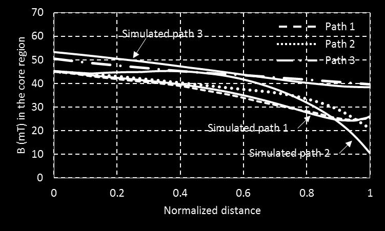
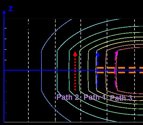
67 (a) (b) (c) Figure Comparison of magnetic flux density along the path shown in Figure 2.10 (a) in the winding region; (b) in the core region; (c) in the fringing region. 46

68 The field is further verified by comparing the energy distributions. The energies stored at different regions are extracted from FES. They are compared to the corresponding energy from the model by integrating B2 over the volume as shown Figure The difference of distribution 2μ percentage between the modeled and simulated energy is less than 3%. When the winding radius is less than one-half of the core radius (Rwo < 0.5Rc), the fringing energy is only around 10% while the winding stores around 80% of the total energy. Therefore, placing the winding near the core radius is beneficial for increasing the energy stored outside the winding area. When the winding is completely outside the core, the model fails to predict the fringing flux accurately from the SC transformation. The error in the fringing energy could be as large as 30%. When the air gap is larger (lg>0.5rc), the flux in the winding area cannot be considered having circular shape. Therefore, the model would overestimate the winding energy by more than 39%. (a) (b) Figure Comparison of energy breakdown between (a) simulation and (b) PREF model for the plate-core inductor with dimensions listed in Table Implementation The pseudo code for the PREF model is demonstrated in this section. 47

69 (1) User defined inputs: core radius, number of turns, core thickness, inner and outer radius of winding window, winding height, width, spacing, air gap length, winding layer spacing, permeability, and current. % Fringing region (2) Define core plate shape in SCgui toolbox and map to strip domain, initialize number of contours Ntot. (3) Plot fringing contours and extract coordinates of each contour. (4) Get initial tangent angle of each flux line: zi f _ i arctan r i (2.29) (5) plot Figure 2.5. % Core region (6) Approximate initialized reluctance. N l tot g i 2 (2.30) R 0 wi (7) Initialize two starting points Rx(i) for the first path. l 2 g Rx(1) Rwi, Rx(2) Rwi 0 i (2.31) (8) Linear function is used for θp: o ( r) 90 (1 r / R ) (2.32) p 0Hy 48

70 (9) Calculate acore and bcore in the elliptical function in (2.5) from a R R b 2 core ( x( i) 0Hy ) core a tan 0.5l 2 core p g R R 0 Hy x( i) 0.5 l ( R R ) g 0 Hy x( i) tan p (2.33) (10) Given r-coordinate R0Hy, solve for z-coordintate Z0Hy from the elliptical function. (11) Solve equations (2.11) - (2.14) numerically with initial guesses of the four unknowns. A maximum of 10 5 iterations and a termination tolerance of 10-3 are set for the solution. (2.34) 4 ini 1 e, ini Rc, ini Z0 Hy, Zc_ ini Z0Hy % Winding region (12) Obtain the boundary angle in the air at the two initial points Rx(i) (i=1, 2) from θp: tan tan ( R ) (2.35) w_ i r p x( i) (13) Solve hwind and Rwind in (2.15) from h tan( ) 0.5 l R, R ( R h ) 0.25l (2.36) 2 2 wind _ i w_ i g x( i) wind _ i x( i) wind _ i g (14) Plot the two complete flux lines starting from Rx(1) and Rx(2). % Reluctance of one path (14) Select (Ninc+1) equally divided points along vertical direction in the winding region, and (Ninc+1) equally divided points along horizontal direction in the core region on the first (i = 1) flux line (e.g. Ninc = 100). 49

71 (15) Find the corresponding points on the second (i = 2) flux line by solving (2.19) and (2.20). (16) Integrate the incremental reluctances in the core and winding region. (17) The corresponding points in the fringing region is given by the SC toolbox, and the fringing reluctance is also found from integrating the incremental reluctances. (18) Calculate total reluctance and flux of the initial path: NI i 2, (2.37) path _ i wind _ i core _ i fring _ i path _ i % Find other flux lines (19) Define an initialized starting point of the next contour R 2 R R ( i 3) (2.38) x(i) x(i 1) x(i 2) (20) Repeat (8)-(18) and adjust the value of Rx(i) until Φ is equal to the one carried by the first path. 2.6 Summary The proportional reluctance, equal-flux (PREF) model is introduced to model the magnetic field distribution for the plate-core inductors with finite core dimension (Rwo Rc). The PREF model is motivated by generating equal-flux lines by making the reluctance of each path proportional to the Ampere-turns. Two elliptical functions, a hyperbolic tangent function, and SC transformations are used to model the shape of the flux lines as guided by FES. The procedure to construct all the flux lines is demonstrated with an example, and the number of total flux lines is governed by the selection of the initial path. The magnetic field at an arbitrary position can be found from these equal-flux paths. Compared to existing modeling method, the error for field 50

72 calculation is reduced to <10% thanks to considering the fringing behavior with finite core dimension. The assumptions in modeling the flux shapes are valid as long as the air gap is small compared to the core radius (lg < 0.5Rc), the winding is close to the core radius (0.8Rc < Rwo < Rc), and the magnetic material has a permeability larger than 5µ0. Based on these limitations, this model is employed in this dissertation to provide the field distribution of plate-core inductors in calculating inductance (see Chapter 3), ac winding losses (see Chapter 4), and core loss (see Chapter 5) within a wide range of geometrical dimensions. 51

73 Chapter 3 Inductance Modeling Nomenclature Symbol Description CM, DM Common model, differential mode condition of field d Vertical distance from middle of gap to the outermost winding layer H mag H r, H z L g L 0 L 11, L 12, L 22 L norm Magnitude of magnetic field Radial and vertical component of magnetic field Air gap length between core plates Base for inductance normalization Inductance matrix parameters Normalized inductance µ, µ r, µ 0 Permeability, relative permeability, vacuum permeability N Turns ratio of primary over secondary R c, H c Radius and thickness of core plate r wi, l g, h c Normalized (to R c) R wi, R wo Inner and outer radius of winding window S layer S ps Vertical distance between winding layers Vertical distance between primary and secondary winding The inductance matrix including self-inductance and mutual inductance of a two-winding inductor is important for circuit simulation (see Chapter 6) to evaluate the voltage waveforms. In this chapter, the derivation of the inductance matrix of inductors with plate-core structure is described. Two conditions are defined as common-mode (CM) field and differential-mode (DM) field in order to compute the matrix parameters. The proportional-reluctance, equal-flux (PREF) model introduced in Chapter 2 is employed to find the CM field distribution, and the DM field distribution is found from functions analogous to that of a solenoid s field [166], [167]. The 52

74 inductance calculated are verified by flex-circuit prototypes with different air gap length, winding radius, and number of turns. The application of the inductance model is presented at the last with normalized parameters to cover structures within a wide range. 3.1 Introduction The magnetic behavior of a two-winding inductor is uniquely represented by an inductance matrix. The energy stored by the inductor is related to the current by * L11 L12 I 1 2E I1 I2 * L21 L 22 I2 (3.1) where L11 and L22 are the self-inductance of the primary and secondary winding, respectively; L12 and L21 are the mutual inductances between primary and secondary. Based on reciprocity theory as proved in [160] and [161], L12 always equal to L21. The inductance matrix is independent of the excitation waveforms, and it is only frequency dependent once the structure is given. Before 1/5 of the self-resonant frequency, the inductance can be considered as a constant value since the phase of the inductor is nearly 90 degrees. The inductance matrix is essential for simulating a two-winding inductor in a circuit because the inductance values and coupling would affect the circuit performance significantly Inductance Matrix Calculation The inductance matrix can be calculated from the field distribution of a two-winding inductor since the energy is the integral of the magnetic field over the volume by 2 B( r, z) 2E dv (3.2) 53

75 In order to solve the three unknowns L11, L12, L22 in the inductance matrix, three energies from three field conditions are needed to calculate the energy. Ideally, any three field-conditions can be employed to solve for the inductance matrix. However, two specific field conditions (CM and DM) and their superimposed field are defined herein for field calculation thanks to the ease of calculation effort because of the symmetry. The first condition is defined as the common-mode (CM) field, where the current in the primary and secondary has the same Ampere-turns and direction as shown in Figure 3.1(a). The energy integrated by the CM field is given by CM : I i, I Ni 2E L i L N i 2L Ni (3.3) where N = N1/N2 is the turns ratio of the primary winding over the secondary winding. z z I 1 N 1 I 1 N 1 I 2 N 2 -I 2 N 2 Common mode (CM): N 1 I 1 = N 2 I 2 Differential mode (DM): N 1 I 1 = -N 2 I 2 (a) (b) Figure 3.1. Definition of (a) common-mode condition and (b) differential-mode condition. r r 54

76 The second condition is defined as the differential-mode (DM) field, where the current in the primary and secondary has the same Ampere-turns but opposite direction as shown in Figure 3.1(b). The energy integrated by the DM field is given by DM : I i, I Ni 2E L i L N i 2L Ni (3.4) The superposition of the CM field and DM field yields the third condition from which the energy is calculated by CM DM : I 2 i, I 0A E 2L i (3.5) Solving the three conditions (3.3) - (3.5), the inductance matrix can be obtained for a twowinding inductor. The next section 3.2 demonstrates the application of the PREF model introduced in Chapter 2 to calculate the CM field, and the DM field calculated is discussed in detail in Section Common-mode (CM) Field Modeling The common-mode (CM) is defined as the condition where the primary and secondary currents have 0-degree phase shift. In order to explore whether the PREF model is applicable for two-winding inductors. The impacts of the number of layers, number of turns, and vertical distance between the layers on the total energy are simulated as below. The radial spacing between the winding turns is used in the PREF when calculating the total Ampere-turns enclosed by a path. However, the vertical distances from winding to winding and from winding to core are not used in the PREF model since the flux line in the winding region is 55

77 almost straight. Two assumptions are used in the PREF model by ignoring the winding layers and vertical distances. First, changing the number of layers should not change the total energy as long as the total Ampere-turns are kept the same. Second, changing the vertical distance between the winding layers (e.g. between two layers) should not change the total energy. In order to verify these two assumptions made in the PREF model, the structure in Table 3.1 was simulated in FES with different number of layers and vertical distances. Since the PREF model gives larger error as the air gap length increases, the structure used herein has the largest air gap allowed (lg = 1/5Rc) that represents the worst case. The number of layers are changed from one to eight as shown in Figure 3.2. The total Ampere-turns are kept at 16 A, and the total energy for each case is shown in Figure 3.2. The structure with only one layer has slightly larger energy (5.6%) compared to the structures with multiple layers because it has no leakage energy between the layers. The small variation in the total energy caused by different number of layers suggests that the PREF model just need to know the total Ampere-turns regardless of the winding layers. The first assumption is verified. In order to verify the second assumption, two-layer structure is used and the distance Slayer between the two winding layers is swept from 0.02 to 0.9 times the air gap length Lg. The total energy with different Slayer is shown in Figure 3.3. The largest variation is only 3.2%, which suggests the vertical distance does not affect the total energy and can be ignored in the PREF model. The second assumption is verified. 56

78 2 A in each turn 1 A in each turn 0.5 A in each turn Total 16 Ampere-turns Total 16 Ampere-turns Total 16 Ampere-turns 0.25 A in each turn Total 16 Ampere-turns Figure 3.2. Impact of number of layers on the total energy with 16 A Ampere-turns and other geometrical dimensions listed in Table 3.1. Figure 3.3. Impact of vertical distance Sps between the winding layers on the total energy with other geometrical dimensions listed in Table

79 Based on the previous two experiments, the field generated by two windings (four layers in Figure 3.4(a)) is equivalent to that generated by a single-winding (two layers in Figure 3.4(b)) with double Ampere-turns. (a) (b) Figure 3.4. Comparison of flux lines between (a) single-winding inductor and (b) two-winding inductor with dimensions listed in Table 2.1. The PREF model discussed in Chapter 2 is employed herein to derive the magnetic field distribution under the CM condition. Figure 3.4 shows that the flux line distribution for a twowinding inductor with double Ampere-turns is the same as that with a single winding. The magnetic field can be calculated by the method discussed in Section The inductance is found from the ratio of total energy over the square of current. Since the place-core structure has a large air gap between the magnetic materials, non-linear behavior of the inductance is ignored for this case. The energy is obtained by integrating the magnetic flux density over the entire volume including the fringing region: L cm 2 2E 1 B( r, z) dv I I (3.6) r 2 Rc, z Lg Hc where B(r, z) is given by (2.2). Compared to (3.3), the inductance calculated from CM condition is given by 58

80 L L L N 2L N (3.7) cm Figure 3.5 compares the CM inductance calculated from (3.6) with the inductance simulated by FEA tools under a wide range of dimensions and geometries. All the dimension parameters are normalized to the core radius Rc since the inductance is scalable with Rc. The inductance are all normalized to the nominal condition given by Table 3.1. The inductance from the PREF model matches very well with simulation results. (a) (b) (c) (d) (e) Figure 3.5. Inductance calculated from (3.6) versus (a) core radius, (b) gap thickness, (c) number of turns, (d) relative permeability, and (e) winding width. Dimensional parameters are normalized to the core radius Rc. When a variable is being swept, the other parameters are kept at the nominal conditions as shown in Table

81 TABLE 3.1. NOMINAL CONDITION OF FIGURE 3.5 Parameter Value Parameter Value Rc 1.7 mm Hc 0.3 mm µ 25 lg 0.34 mm Number of turns 16 Winding width 50 µm 3.3 Differential-mode (DM) Field Modeling The differential mode is defined as the condition where the primary and secondary winding carry the same Ampere-turns, but opposite direction. The modeling of DM field uses equations analogous to the field of a solenoid [166], [167] after simplifying the structure into no-spacing structure. The validity of using the simplified structure to find the field is verified parametrically. The DM inductance Ldm is found from the DM energy, which is the integral of the field Simplified Structure without Spacing As shown in Figure 3.6(a) and (c), the field distribution under this condition is very nonuniform and hard to model accurately. Therefore, the simplified structure shown in Figure 3.6(b) and (d) is employed to calculate the inductance in order to simplify the problem. The simplified structure has the same inner and outer radius as the original structure, but the spacing between the turns are eliminated such that it becomes a combined multi-layer structure. The current is assumed uniformly distributed along the conductor layer, and the field from the simplified structure is more uniform than that of the original structure as shown in Figure 3.6(d). The validity of the simplified structure to replace the original structure is verified over wide range. The inductance from the DM condition of the original structure is compared to that of the simplified structure while geometrical parameters, such as winding inner radius, turn-turn spacing, vertical spacing between the primary and secondary winding, permeability, core height, winding 60

82 height, and number of turns, are swept. Figure 3.7 suggests that the inductance of the two structures match very well, and it is valid to replace the original structure by simplified structure for inductance calculation. Structure with spacing Structure without spacing 16 A -16 A d R wi 1 A in each turn R wo 16 A d -16 A R wi 8 A in each layer NI S ps R wo L g (a) Non-uniform field distribution (b) Uniform field distribution Rwi = 0.9 mm, Rwo = 1.65 mm, 16 turns per layer, Lg= 0.34 mm, Rc = 1.7 mm, Hc = 0.3 mm, µ = 25 R wi = 0.9 mm, R wo = 1.65 mm (c) (d) Figure 3.6. Comparison of magnetic field distribution Hmag between (a) original plate-core structure with 16 turns on each layer, and (b) simplified no-spacing structure with dimensions in Table 3.1. (a) (b) 61

83 (c) (d) (e) (f) (g) Figure 3.7. Comparison of leakage inductance between original plate-core structure and the corresponding simplified structure with no spacing as shown in Figure 3.6, parametric with (a) inner winding radius, (b) spacing between winding turns, (c) spacing between primary and secondary windings, (d) material permeability, (e) core thickness, (f) winding height, and (g) number of winding turns. 62

84 3.3.2 Methodology In order to model the DM field, the radial field component Hr along the radial line rr is found first using the function [166], [167] below at the vertical middle between primary and secondary windings (z = 0): NI r Rwi r R wo Rwo Rwi Hr ( r, z 0) (0 r ) 2(R R ) wo wi (r R ) (r R ) 2 wi d wo d (3.8) where NI is the Ampere-turns; Rwi and Rwo are the inner and outer winding radius, respectively; d is the distance between the center of the structure to the outermost winding layer as shown in Figure 3.8. The equation is similar to that of a solenoid in the x-y plane. The horizontal coordinate x becomes radius r when the equations is applied to the cylindrical plane. Figure 3.8. Parameters used for calculating radial field component Hr along radial line rr. The vertical field component Hz along the radial line rr is then calculated by drawing different Ampere-loops at a given r-coordinate as shown in Figure 3.9. l g /2 0 Rwo r H z( r, z) dz Hr( r) dr NI R R (3.9) r wo wi 63

85 where the vertical field component Hz along the vertical line zz is assumed to be piecewise linear at a given r-coordinate: l g /2 lg S ps H z ( r, z 0) S ps lg S ps H z ( r, z) dz H z ( r, z 0) ( ) ( ) H z ( r, z 0) ( ) (3.10) Figure 3.9. Parameters used for calculating vertical field component Hz along radial line rr and vertical line zz. The radial field component Hr along the vertical line zz is assumed uniform between the winding layers and changes with the number of layers. The modeling results of the radial and vertical field components Hr and Hz along radial line rr and vertical line zz are shown in Figure 3.10(a) (d). by The magnitude of the magnetic field can be calculated from the radial and vertical components H r z H r z H r z (3.11) 2 2 mag (, ) r (, ) z (, ) 64

86 Vertical magnetic field Hz (A/m) Vertical magnetic field Hz (A/m) Radial magnetic field Hr (A/m) Radial magnetic field Hr (A/m) Simulation Model Simulation Model Distance along rr (m) (a) Distance along zz (m) (b) Simulation Model Simulation Model Distance along rr (m) Distance along zz (m) (c) (d) Figure (a) Hr field along r-direction, (b) Hr field along z-direction, (c) Hz field along r-direction, and (d) Hz field along z-direction for simplified structure with no spacing with dimensions listed in Table 3.1 and parameters labeled in Figure 3.8. The modeled Hmag resulted from solving the equations (3.8) - (3.10) is shown in Figure 3.11(b). Compared to the simulated DM field, the modeled field has very similar pattern and the difference is 9.3%. The error is mainly caused by the assumption that the Hr remains constant between the two windings along the vertical direction. 65

87 Simulated DM H field 16A -16A (a) Modeled DM H field 16A -16A (b) Figure Comparison of (a) simulated magnetic field Hmag in FES and (b) modeled magnetic field Hmag under DM condition with dimensions listed in Table 3.1. The inductance is found from the ratio of total energy over the square of current. The energy is obtained by integrating the magnetic flux density over the entire volume including the fringing region L dm 2 2E 1 B( r, z) dv I I (3.12) r 2 Rc, z Lg Hc Compared to (3.4), the inductance calculated from DM condition is given by L L L N 2L N (3.13) dm

88 The DM inductances calculated from (3.12) using the methodology discussed in this section for different parameters are compared to the FES results with separate turns and simplified structure without spacing. The comparison of results are shown in Figure The model matches with the simulation results very well with less than 10% error, as long as the µ is larger than 5 and Rc/lg is larger than 5 as required by the PREF model. When the µ or the Rc/lg is smaller than 5, the assumption where the Hr remains constant along vertical-direction becomes invalid since the field is no longer constrained by the core plates. The Matlab code is documented in Appendix D. (a) (b) (c) (d) (e) (f) Figure Modeled DM inductance calculated from (3.12) using simplified structure without spacing versus (a) inner winding radius, (b) spacing between primary and secondary windings, (c) winding height, (d) air gap length, and (e) permeability compared to FES with original 16-turn structure. The other parameters are kept at the nominal conditions as shown in Table 3.1 when one parameter is varied. The third field condition is the sum of the CM field and the DM field. The magnetic fields versus space calculated from the CM and DM conditions are added together to get the field 67

89 distribution where only primary winding is conducting and the secondary winding is open. Compared to (3.5), the inductance calculated from CM+DM condition is given by L cm dm L 11 (3.14) The final inductance matrix L11, L22, and L12 for a two-winding inductor can be obtained by solving (3.7), (3.13), and (3.14). The inductance matrix is verified by experimental results in the next section, and the pseudo codes to derive the three field conditions are shown in Section Error! Reference source not found Experimental Verification In order to verify the inductance matrix calculated, several winding layouts with different variables and inductances were fabricated and measured to verify the inductance modeling results for 1:1 two-winding inductors. The prototype shown in Figure 3.13 consists of a 3 4 inductor matrix with the purpose to verify different parameters. The thickness of one winding layer was 0.25 mm, and two identical winding layers were stacked together to make a two-winding inductor. Therefore, the total thickness of the winding layer became 0.5 mm, which formed the air gap between the two core plates. The first row had the same winding layouts, but the air gap length was varied from 0.5 mm to 1 mm with 3-mm Rwi and 8 turns on each layer. The second row kept the air gap length at 0.5 mm, but varied the inner radius from 1 mm to 3.7 mm by varying the winding width under the same number of turns. The third row varied the number of turns under two Rwi while keeping the air gap length at 0.5 mm. The fabricated flexible circuit shown in Figure 3.15 had 18-µm-thick copper layer on both sides; the polyimide thickness between the copper layers was 2 mils; and the total thickness of one 68

90 TABLE 3.2. DIMENSIONS OF INDUCTOR PROTOTYPES No. Rwi (mm) Lg (mm) N/layer Wwidth (µm) Rc = 5 mm, Hc = 0.3 mm, turn-turn spacing = 3 mils, Rwo = 4.95 mm, winding layer spacing = 2 mils, winding thickness = 18 µm, µ = 80µ0. 1 st Row - vary air gap: N = 8, Rwi = 3 mm Lg = 0.4 mm Lg = 0.5 mm Lg = 0.75 mm Lg = 1 mm 2 nd Row - vary Rwi: N = 8, lg = 0.25 mm Rwi 1 mm 2 mm 3 mm 3.7 mm 3 rd Row - vary number of turns: lg = 0.25 mm N = 6 N = 4 N = 6 N = 4 Rwi = 3 mm Rwi = 2 mm Figure Layouts of winding matrix fabricated with flexible circuit for inductance verification. 69

91 winding sheet was 0.25 mm as half of the air gap distance. The round plate-core shown in Figure 3.15 was made of 4F1 material, and it was customized to a diameter of 10 mm and a thickness of 0.3 mm. The core plates were attached to the top and bottom side of the flexible circuits as shown in Figure However, the prototype was too flexible to form a solid structure. Therefore, two fixtures made of 1-mm-thick FR4 material were fabricated to sandwich the flexible circuits and increase the rigidness. Two masks with cavities for the cores were added to the top and bottom of the flexible circuit in order to maintain a stable air gap length between the two core plates. The round core plates were inserted to the holes on the masks and stabilized by Kapton tape. The assembled prototype used for testing is shown in Figure (a) Figure Prototype of one inductor layout (a) top view and (b) side view. (b) In order to minimize the parasitic impedance introduced by the testing fixture, a customized four-terminal testing fixture was fabricated. The layout of the fixture is shown in Figure 3.16(a). Four BNC connectors with 22-mm distance between each other were used to connect the fixture 70

92 to the four terminals on the Impedance Analyzer [168]. A right-angled header was used to connect the fixture to the inductor prototype by Kelvin connection as shown in Figure 3.16(b). Figure Assembly process of two-winding inductor prototype using two layers of flexible circuits, ferrite core material, and two masks. (a) (b) Figure (a) Customized four-terminal testing fixture and (b) an exemplary layout of the inductor on the flexible circuit. 71

93 The prototype with inductor matrix is measured by Impedance Analyzer 4294a from Agilent, and the testing setup is shown in Figure The customized testing fixture was first calibrated with open and short condition, and then the initial inductance of each layout was measured and compared to the simulation and modeling results. Figure Testing setup of inductor prototype using customized testing fixture and Impedance Analyzer [168]. The initial inductance of each layout is measured and compared with the FES and PREF model as shown in Figure The inductance measured with open secondary-side is related to the inductance matrix parameters by Lopen L (3.15) 11 For all the parameters tested, the measurement shows less than 16% variance with the simulation and modeling results. The calculation results from PREF agrees very well with FEA in Figure 3.18 (a) and (c), and the error between measurement and FEA is mainly caused by the 72

94 measurement error in the air gap length and fabrication deviation; the error in Figure 3.18(b) between PREF model and the FEA (or measurement) is mainly from the numerical solution errors in solving the shapes of the contours. (a) (b) (c) Figure Comparisons of measured open-inductance with FES and modeled results under different (a) air gap length, (b) winding inner radius, and (c) number of turns. The short inductance of each layout is measured by shorting the secondary side. The inductance measured with shorted secondary-side is related to the imaginary part of the impedance matrix by L short 2 Z12 Im( Z11 ) (3.16) Z 22 73

95 Lshort (nh) Lshort (nh) Lshort (nh) The measured results are compared with the FES and modeled result as shown in Figure For all the parameters tested, the measurement matches well with the simulation and modeling results with less than 6% variance Air gap length (mm) Inner winding radius (mm) (a) (b) Number of turns per layer (c) Figure Comparisons of measured short-inductance with FES and modeled results under different (a) air gap length, (b) winding inner radius, and (c) number of turns. 3.5 Exemplary Utilization of Model Normalization of the self-inductance and the dimensions of plate-core inductors is discussed in this section to demonstrate plots that are valid for a wide range. Based on numerical simulation results with different number of turns (by changing winding width) and minimal spacing (5 µm) 74

96 between the turns, the nominal inductance L/N 2 is a constant value as shown in Figure 3.20(b) with a given winding inner radius Rwi. Therefore, the inductance is only related to the winding window area, and it can be normalized to a base inductance L0: L N R (3.17) c where µ0 is the vacuum permeability, N is the number of turns, and Rc is the core radius. z Example structure: µ H c L g Rwi R c (a) (b) Figure (a) Plate-core structure used for inductance synthesis and (b) nominal inductance (L/N 2 ) versus number of turns with Rwi = 0.9 mm and Rwo = 1.65 mm for the structure in Table

97 The normalized inductance Lnorm = L/L0 as the output is independent of the number of turns and scalable with the core radius Rc. The other variables include inner winding radius Rwi, air gap length Lg, core thickness Hc, and material permeability µ as listed in Table 3.3. The inductance is most sensitive to the inner winding radius, so the sweeping range of Rwi spans from 0.01Rc to 0.9Rc. Considering the limitation of the PREF model, the upper limit of Lg is set to 0.2Rc and the lower limit of the relative permeability is set to 5. The core thickness Hc can be as low as 0.01Rc for thinfilm materials and as high as 0.5Rc for bulk structures. TABLE 3.3. SWEEPING RANGE AND NOMINAL VALUES OF PARAMETERS Output Base of normalization Normalized output L L 0 = µ 0N 2 R c L norm = L/L 0 Variables Normalized Base of normalization Normalized range Nominal value R wi r wi R c L g l g R c (l g<1/5r c) 0.1 H c h c R c µ µ r µ The sweeping plots of Table 3.3 are shown in Figure The vertical axis is the normalized inductance and horizontal axis is the normalized inner winding radius. Each plot shows several curves parametric with hc, lg, and µ. Figure 3.21(a) shows that the inductance increases with rwi and hc. However, when hc is larger than 0.5, the increase of inductance is minimal and the core thickness is no longer a key factor affecting the inductance. Figure 3.21(b) shows that the inductance increases with rwi but reduces with lg. Similarly, the decrease of inductance is minimal when the normalized air gap lg is larger than 0.15 since the air gap is too large to affect the inductance severely. Figure 3.21(c) shows that 76

98 (a) (b) (c) Figure Relationship between the normalized inductance and the normalized inner winding radius parametric with normalized (a) core thickness, (b) air gap length, and (c) relative permeability with the parameters in Table

99 the inductance becomes almost two times larger when the permeability increases from 5 to 25, but varies less than 20% when the permeability increases from 50 to Implementation The pseudo code for the inductance calculation is demonstrated in this section. (1) User defined inputs for a two-winding inductor: core radius, number of turns on each side, core thickness, inner and outer radius of winding window, winding height, width, spacing, air gap length, winding layer spacing, primary to secondary vertical spacing, permeability, and currents. % CM field (2) Follow the steps (2) (20) in Section Error! Reference source not found. to generate the flux lines considering the total Ampere-turns in both windings. (3) Generate a mesh grid [r, z] within the region Zp z Zp + Hc and 0 r 2Rc for field calculation. (4) Determine the two flux lines Φi and Φi+1 that sandwich each point in the mesh grid. (5) Find the B at each point (r0, z0) in the mesh grid by % DM field B 1 r z r z B r r B z z (3.18) i i 1 i i 1 ( 0, 0) ( ) r0 zi zi 1 ri ri 1 (6) Find Hx distribution along r-direction from 0 to (Rwo+Rwi)/2 in the middle of the vertical spacing between the primary and secondary windings (z = 0) by NI r Rwi r R wo Rwo Rwi H x ( r, z 0) (0 r ) 2( R ) wo Rwi ( r R ) ( ) 2 wi d r Rwo d 78 (3.19)

100 (7) Flip the Hx distribution based on symmetry axis r = (Rwo+Rwi)/2 to get the complete distribution of Hx from r = 0 to r = Rc. (8) Find Hy distribution along r at z = 0 by sweeping r from 0 to Rwo: Rwo r lg Sps H y( r, z 0) ( NI H x( r) dr) / ( ) R R (3.20) 2 4 wo wi r (9) Find Hx and Hy distribution at z 0. Hx (r, z) is scalable to Hx(r, z = 0) based on the Ampereturns enclosed; Hy (r, z) is approximated by piesewise-linear function to Hy (r, z=0) given by (3.10). (10) Generate a same mesh grid [r, z] within the region Zp z Zp + Hc and 0 r 2Rc. Obtain the field at each point in the grid based on steps (6) (9). % CM+DM field (11) Adding the B matrix generated in step (5) to the B matrix in step (10) with the same mesh grid to get the B matrix of CM + DM field. (12) The energy with the CM, DM, and CM + DM can be calculated from the integration of the B matrix in step (5), (10), and (11) over the mesh volume, respectively. (13) Extract inductance matrix L11, L12, and L22 from (3.3) (3.5). 3.7 Summary The inductance matrix of a two-winding inductor determines the circuit performance of the magnetic component. The calculation of the inductance matrix is discussed in this chapter. The three unknowns L11, L12, and L22 of a matrix can be determined from the energies integrated from three field conditions defined as the common mode (CM), the differential mode (DM), and the superposition of the previous two modes (CM+DM). The CM field is modeled by the PREF model 79

101 introduced in Chapter 2, and the DM field is calculated from functions analogous to the field of a solenoid and Ampere s Law. The modeling of CM and DM field, energy, and inductance are verified by FES results with normalized air gap length, inner winding radius, permeability, and number of turns. The limitations of CM and DM inductance calculations are the same as those of the PREF model where Rc/Lg and permeability should be larger than 5. When the permeability is too low and the air gap is too large, the assumptions of the flux shape in the gap area become invalid. Two-winding inductor prototypes made of flex-circuits are used to verify the modeling results and simulation results from FEA. The inductances with open and short secondary are measured by Impedance Analyzer that show good agreement (less than 10% error) with the calculation and simulation. The calculation of the inductance is generalized by normalizing it to a base function that is scalable with the number of turns and core radius. A parametric study is carried out to show the impact of normalized inner winding radius rwi, core thickness hc, normalized air gap length lg, and relative permeability on the inductance. The inductance is dominated by rwi and increases when rwi approaches Rc. The inductance becomes almost stable when hc > 0.5, or lg > 0.15, or the permeability is larger than

102 Chapter 4 Winding Loss Modeling Nomenclature Symbol Description CM, DM Common model, differential mode condition of field δ Skin depth F ac H x, H y H eddy H x(a), H x(0) H y(0), H y(h) J 1 J 2 J eddy J dc k K u L g Ratio of ac resistance to dc resistance Horizontal and vertical magnetic field, equivalent to H r and H z in cylindrical plane Eddy-current field that penetrates the conductor top and bottom surfaces Horizontal field along the top and bottom surface of a conductor Vertical field along the left and right surface of a conductor Current density variation caused by vertical field Current density variation caused by horizontal field Current density variation caused by eddy-current field Dc current density distribution Ratio of ac current to dc current Copper fill factor of winding window Air gap length between core plates µ, µ r, µ 0 Permeability, relative permeability, vacuum permeability N Turns ratio of primary over secondary R 11, R 12, R 22 Resistance matrix parameters R c, H c Radius and thickness of core plate R wi, R wo Inner and outer radius of winding window S layer S ps Vertical distance between winding layers Vertical distance between primary and secondary winding x, y Horizontal and vertical coordinates, equivalent to r and z in cylindrical plane w Winding width In circuit where two-winding inductors are used instead of transformers, the phase shift between the primary and secondary side is not always 180 degrees. Therefore, it is important to 81

103 model the winding loss for a two-winding inductor accurately. The winding loss can be calculated from the resistance matrix, which is independent of excitations but only relates to the frequency and geometry. The methodology to derive the resistance matrix from winding losses of twowinding inductors is discussed in the chapter. Winding loss model with 2D magnetic field is improved by including the additional eddy current loss for better accuracy for the plate-core structures. The valid range of the improved model is explored with normalized winding width and height. The error is less than 10% as long as the winding width and height is smaller than ten times and five times the skin depth, respectively. The resistance matrix calculated from the model is verified by both measurement results and finite-element simulation (FES) of two-winding inductor prototypes. 4.1 Introduction The winding thickness for planar magnetic components is pre-determined by the copper thickness on the pcb. Therefore, the current capability is mainly determined by the width of the winding turns. As the operating frequency of power converters becomes higher and higher, it is important to have an accurate method to predict the winding loss caused by the skin effect and proximity effect Resistance Matrix of Two-winding Inductor The winding loss of a two-winding inductor is uniquely determined by its resistance matrix. For each harmonic current, the resistance matrix relates the rms value of the sinusoidal current to the winding loss by * R11 R12 I 1 P loss I1 I2 * R21 R 22 I2 (4.1) 82

104 This can also be written as P I R I R ( I I R I I R )cos (4.2) 2 2 loss 1, rms 11 2, rms 22 1, rms 2, rms 12 1, rms 2, rms 21 where θ is the phase angle between I1 and I2, and R12 equals R21 based on reciprocity theorem [160]. The resistance matrix is independent of the magnitude of the current, and is only related to the geometry and the frequency of the harmonic current. An arbitrary current can be decomposed into several harmonic current with sinusoidal waveform by Fourier transform, and the total winding loss is obtained from the sum of the winding loss under each harmonic frequency ωi: 2 2 loss, tot 1, rms _ 11_ 2, _ 22_ 2 1, _ 2, _ 12_ cos i i rms i i rms i rms i i _ i i 1 P I R I R I I R (4.3) Similar to the inductance matrix calculation in Section 3.1.1, the three unknowns R11, R12, and R22 for each harmonic frequency can be determined from the winding loss of three conditions. Single frequency is assumed for the winding loss model in this chapter. For calculation simplicity, the first condition is the winding loss calculated with the CM field: CM : I i, I N i P R i R N i 2R Ni (4.4) where N = N1/N2 is the turns ratio of the primary winding over the secondary winding. The secondary condition is the winding loss calculated with the DM field: DM : I i, I N i P R i R N i 2R Ni (4.5) The superposition of the CM field and DM field yields the third condition from which the winding loss is calculated by 83

105 CM DM : I 2 i, I 0A P R i (4.6) After obtaining the field distributions for the CM and DM conditions from the method discussed in Chapter 3, the winding losses can be found from the field by the improved model introduced in this chapter D Magnetic Field around Winding Turns The most classical way to calculate the copper loss of multilayer transformers is the 1D solution to the Maxwell s equations by Dowell [57]. The following assumptions are made for the classical 1D condition: 1) the magnetic field inside the core can be considered to be zero; 2) the magnetic field is parallel to the conductor layers, and the field only has one direction along the y-axis for vertical layers or along x-axis for horizontal layers; 3) the current density inside the winding layer only changes along the x-axis and remains constant along the y-axis. These assumptions are valid for transformers with multiple layers [58]-[69] where the permeability of the core is large, the window fill factor is high, and the edge effect [70] - [77] can be ignored. However, these assumptions are not valid for the plate-core structure exemplified in Figure 4.1. The magnetic field for the structure in Figure 4.1 is shown in Figure 4.2. The magnitude of the magnetic field along the horizontal (Hx) and vertical (Hy) directions are comparable to each other, suggesting the magnetic field distribution is 2D. The 2D effect becomes more obvious when the air gap becomes larger since there is considerable spacing between the winding layers and the core plates. Therefore, the winding loss model for the plate-core structure requires 2D solution. 84

106 z R c = 1.7 mm H c = 0.3 mm R wi = 0.9 mm R wo = 1.65 mm L g = mm Winding width/spacing = 50/50 µm Winding layer spacing = 35 µm r Figure 4.1. Example structure of plate-core inductor with single winding. H x magnitude H y magnitude (a) (b) H x vector H y vector (c) (d) Figure 4.2. Simulated 2D field (a) Hx magnitude, (b) Hy magnitude, (c) Hx vector, and (d) Hy vector for structure shown in Figure

107 4.1.3 Conventional Models for 2D Winding Loss Many existing methods [57] - [85] try to calculate the winding loss including the 2D effect. The edge effect discussed in [70] - [77] considers the 2D flux at the end of a winding turn where the strip is not infinitely long as assumed in the 1D solution. The winding loss calculation is adjusted by adding a correction factor to the Fac of the original 1D solution. Two-dimensional and three-dimensional winding loss are calculated in [72] for round wires with diameters no more than the skin depth by generating the matrix reflection between the field and the loss. Numerical results showing the relationship between the 2D field and the loss with different geometrical factor are presented in [73]. Closed-form analytical equation for winding loss by solving the second-order diffusion equation can be found in [74] with the assumption that the field flows parallel to the surfaces. The effect on the winding loss of the fringing effect from the air gaps is discussed in [78]-[81] by introducing additional eddy loss equations. A 2D winding loss using superposition of the current density caused by the field on x-direction and y-direction separately is introduced in [81]. The model is used for the closed-core structure as shown in Figure 4.3, where the flux is constrained by the magnetic core and the direction of the flux is always parallel to the conductor surfaces. For inductors in Cartesian coordinates, the x, y, and z axis are defined in the way labeled in Figure 4.3. The cross-section of the conductor is in the x-y plane, and the current flows in the z-direction. The inductors in cylindrical coordinates, the x, y, and z axis become r, z, and ϕ axis, respectively. As long as the curvature of a winding ( R i /R o 1) is small, the solution is the same as in the Cartesian coordinates [64], [154]. The assumptions for the 2D winding loss model include 1) flux is parallel to the conductor surfaces; 86

108 2) Hy only changes along the x-axis, Hx only changes along the y-axis; 3) only Jz exists, and it changes along x-axis and y-axis. y z Hx(a) h a Parallel flux around windings Hy(0) Hy(h) Jz Jz Jz Jz Jz Jz Jz Jz Hx(0) x Figure 4.3. Closed-core structure used for conventional 2D winding loss model with parallel flux to the surfaces. current: This 2D winding loss model is derived from the Maxwell equation ignoring the displacement Β E t Η J E (4.7) Based on the second and third assumptions where Hy only changes along the x-axis, Hx only changes along the y-axis, and only Ez exists, the equations can be simplified as dez( x, y) dez( x, y) E 0 j ( H y( x) H x(y)) dy dx dh y ( x) dh x( y) H J z( x, y) Ez( x, y) dx dy (4.8) When Hy is considered as the variable, Hx is considered as a constant boundary condition. The variation in Ez is one-dimensional since it only caused by Hy(x): 87

109 dez( x) dez( x) 0, 0 j H y ( x) (4.9) dy dx Replace Hy in (4.8) by (4.9): ( x) 1 Hx(a) Hx(0) Ez ( x, y) dx j a 2 d Ez 2 2 d J z 2 0 ( x) 1 Hx(a) Hx(0) J1( x) J dx j a 0 dc (4.10) Similarly, if Hx is considered as the variable, Hy becomes the boundary condition: ( y) 1 Hy(0) Hy(h) J2( y) Jdc (4.11) dy j h 2 d J z 2 0 where Hx(a), Hx(0) are the horizontal boundary field along the top and bottom surface of the conductor; Hy(0), Hy(h) are the vertical boundary field along the left and right surface of the conductor; a is the conductor height; and h is the conductor width as shown in Figure 4.3. J1(x) is the eddy current density induced by Hy and only has x-variation; J2(y) is the eddy current density induced by Hx and only has y-variation; and Jdc is the uniform dc current density inside the conductor given by Jdc = I/a/h. is Solving the second-order derivative equation (4.10), the current density along the x-direction 2 J 1( x) P cosh(kx) Q sinh(kx) J dc (4.12) where 88

110 j H (0) H (a) H (h) H (0) cosh(kh),,, (0) (4.13) a sinh(kh) 0 x x y y k 1 P1 k Q1 kh y Similarly, solving the current density along the y-direction from (4.11) is 2 J2( y) 2 P2 cosh( ky) Q2 sinh( ky) J dc (4.14) where Hy(0) Hy(h) H x(a) H x(0) cosh( ka) 2, P2 k, Q2 kh x(0) (4.15) h sinh( ka) The total current density is the superposition of the J along the x-direction and the y-direction: J J1 J2 Jdc (4.16) The winding loss is found from the surface integration of current density: Pac 1 J J dxdy 2 (4.17) This 2D winding loss model (referred as conventional model in later sections) is applied to the plate-core structure as it is derived from the Maxwell s equations and includes the field impact on both directions. Figure 4.4 compares the calculation results using (4.12) - (4.17) with the simulation results for the plate-core inductor shown in Figure 4.1 with different winding width. The boundary fields used in (4.13) and (4.15) are derived from the PREF model and verified by FES. However, the 2D winding loss model gives a large error when the winding width becomes larger than the skin depth as shown in Figure

111 Simulated loss Figure 4.4. Comparison of simulated total winding loss and calculated loss using (4.13) - (4.17) for the structure shown in Figure 4.1 with variable winding width under 1 A current excitation at 5 MHz. The winding loss distribution in each turn when the width is 80 µm (see Figure 4.4) is compared to the simulation results in Figure 4.5(a). The calculated winding loss is always smaller than the simulated winding loss, especially for the innermost and outermost winding turns. Figure 4.5(b) compares the winding loss in the first turn when the winding width is changed from one skin depth to four times skin depth, and the error between simulation and calculation can be as large as 65% (see Figure 4.5(b)). 4.2 Winding Loss Calculation with Additional Eddy Current Loss The error shown in Figure 4.5 comes from the assumption that the flux is parallel to the conductor surface in the conventional model. An additional eddy current loss is introduced by the fringing flux when the winding turns are placed directly in the air gap area. 90

112 Winding loss in first turn (W) Ploss (W) 0.15 Winding loss in each turn when width = 80 um Pac_cal Pac_sim (a) Simulated loss Calculated loss Normalized w/δ (b) Figure 4.5. Comparison of (a) simulated winding loss and calculated loss in the first turn for the structure shown in Figure 4.1 with 80 µm winding width, (b) winding loss in the first turn versus normalized winding width to skin depth between simulation and calculation Additional Eddy Effect in the Windings The 2D winding loss model underestimates the actual winding loss because there is flux penetrating the conductor surface for the plate-core inductors as shown in Figure 4.6. The flux in the air gap has no magnetic material to shape the pattern such that the flux penetrates the conductor surfaces. Contradictory to the assumptions in the conventional 2D winding loss model, the flux is 91

113 not always parallel to the surface but orthogonal to the conductor. This will cause additional eddy current loss due to the circulating current inside the conductor [78] - [80]. It should be noted that only one-dimensional eddy current loss caused by the vertical flux is considered herein, and the horizontal flux penetrating the conductor is ignored. This is because the pcb windings usually have low profile and the thickness is less than one skin depth, and the effect on the current density distribution from the horizontal penetrating flux is small enough to be ignored. H eddy H y(0) H x(a) Boundary field H y(h) H x(0) Flux not parallel Figure 4.6. Flux around the winding turns of plate-core inductor showing vertical flux penetrating the winding surfaces. Therefore, besides the skin effect and proximity effect modeled in the 2D winding loss model, an additional term is added to the total current density caused by the penetrating field: J J J ( x) (4.18) skin prox eddy The Jy caused by vertical flux is related to an effective eddy field Heddy by [79] J eddy j Heddy x ( x) (4.19) 92

114 4.2.2 Normalized Function for Eddy Current Loss Modeling the eddy current loss accurately is essential to improve the conventional 2D winding loss model for the plate-core inductors. The effective Heddy used in (4.19) is assumed constant over the conductor surface, and it should predict the Jy accurately for the loss calculation. Figure 4.7 shows the vertical field distribution across each winding turn when the frequency changed from 0 Hz (dc condition) to 10 MHz with 1 A current in each turn. The field distribution is not a constant even at dc condition, and it becomes more non-uniform under higher frequency. In addition, the field distribution is impacted by the frequency, suggesting that Heddy should be frequencydependent. field under dc Hy field (A/m) 2 MHz - 10 MHz H y distribution along this line H y0 H eddy H yh Distance (mm) Figure 4.7. The non-uniform magnetic field Hy distribution along x-direction across the windings in Figure 4.1 with 1A current under 0 to 10 MHz frequencies. The objective of generating a normalized function for the eddy current loss calculation is to have a model for the Heddy that effectively predicts the eddy current density Jy with frequencies and dimensions in wide range. 93

115 Considering most of the flux is vertical in the air gap area as shown in Figure 4.6, the width of the winding is a dominant parameter that affects the eddy current loss. The winding width is normalized such that frequency impact is included in the calculation. The dc fields Hdc in Figure 4.7 can be obtained from the PREF model, and they are used to find the effective Heddy field. Each winding turn has different Hdc (see Figure 4.7) resulted from the winding dimension, air gap length, and core dimension. The assumption is that the ratio of Heddy to Hdc of each turn is a constant function that only depends on the normalized (to skin depth) winding width w/δ. The procedure to extract the ratio of Heddy to Hdc versus w/δ is summarized as follows. First, a winding turn (e.g. the innermost turn 1 in Figure 4.1) from a random plate-core structure is selected as the object to extract the function. The boundary field Hy0 and Hyh under dc condition for this turn can be obtained from either the FES or the PREF model. Second, the simulated loss under different frequencies for this turn is recorded, and the Heddy is tuned for each frequency until the calculated loss from (4.18) and (4.19) matches the simulated one. Finally, the Heddy is normalized to the dc boundary field, and numerical function is searched for the eddy field in terms of the normalized width divided by the skin depth: H dc Hy0 Hyh (4.20) 2 H w w w w (w 5δ) (4.21) eddy / Hdc ( ) ( ) ( ) ( ) The curve-fit function (4.21) for the eddy field is shown Figure 4.8 for normalized winding width from 1 to 5. This generalized function only depends on the normalized winding width, and it should work for all the winding turns although it is derived from one specific turn. The impact 94

116 of different field distribution around different turns is included in the Hdc, to which the Heddy is normalized. Eddy factor H eddy /H dc H eddy normalized to H dc y = x x x x R² = Normalized winding width (w/δ) Figure 4.8. Curve-fit function for the eddy factor versus normalized winding width from 1-5. Compared to the original 2D winding loss model in (4.16) and (4.17), the improved winding loss model adds an additional eddy current term to the total current density: J J ( x) J ( y) J ( x) J (4.22) 1 2 eddy dc where Jeddy(x) is calculated from (4.19) - (4.21). The winding loss is found from the integration of the current density by Pac 1 J J dxdy 2 (4.23) After adding the additional eddy current loss to the calculation, the winding loss in the first turn matches very well with the simulation results as shown in Figure

117 Solid: simulation Dash: calculation Figure 4.9. Comparison of winding loss in the first turn of Figure 4.1 with 1A current excitation under 1 10 MHz frequency after including the eddy factor. By following the same procedure, the function of eddy field for a wider range of normalized winding width from 1 to 10 can be obtained as shown in Figure Eddy Factor H eddy /H dc H eddy normalized to H dc y = x x x x x x R² = Normalized winding width (w/δ) Figure Curve-fit function of eddy field versus normalized winding width from 1 to

118 The loss in each turn under 1 MHz, 5 MHz, and 10 MHz calculated using (4.12) - (4.23) for the structure in Figure 4.1 is compared to the simulation as shown in Figure The winding loss model is accurate in a wide frequency range thanks to the wider range function of eddy field. The Matlab code for the improved winding loss model is documented in Appendix E. 4.3 Valid Range of Improved Winding Loss Model In order to explore the valid range of the winding loss model and the function for the eddy factor, statistical method is used to find the response surface model to predict the expected error between the calculated and simulated winding loss. The parameters involved and their variation range are summarized in Table 4.1. TABLE 4.1. NORMALIZED RANGE OF PARAMETERS Defined variables Range of variation Base of normalization Normalized range N per layer Winding inner radius Rwi mm R c = 5 mm Turn-turn spacing s µm δ (at 5 MHz) = µm 1 10 Winding width w µm δ (at 5 MHz) = µm 1 10 Gap length Lg mm R c = 5 mm Winding layer spacing Slayer µm δ (at 5 MHz) = µm 1-5 Winding height h µm δ (at 5 MHz) = µm Core thickness Hc mm R c = 5 mm

119 1 MHz simulation calculation 5 MHz simulation calculation 10 MHz simulation calculation Figure Comparison of loss breakdown in each turn between simulation and calculation with 1 A current excitation at 1 MHz, 5 MHz, and 10 MHz for the structure in Figure

120 The experimental settings needed to generate the model were generated by JMP [163], and each experiment was run in both Maxwell and Matlab. The differences between Maxwell and Matlab calculated result were recorded as the output: Err R R (4.24) R ac _ sim ac _ cal % 100 ac _ sim These outputs were fit into a response-surface model by numerical regression in JMP. The response-surface model is used to predict the calculation error for a set of given inputs. Figure Input and output parameters for response-surface model in statistical software. The experimental data was analyzed by JMP to find the most sensitive parameters that increases the error between the calculation and simulation. The significance level of each input parameter and their second-order interactions were analyzed, and the parameters are listed in the order of p-value [163] in Figure When the p-value is smaller than 0.05, the parameter has significant impact to the output as shown in Figure 4.13 in the red color with an asterisk. The error is most sensitive to the winding height since only the eddy current field penetrating the conductor width is considered in the improved model. When the winding height is significantly larger than the skin depth, the eddy current factor along the horizontal direction also needs to be considered. 99

121 However, that will further increase the complexity of the calculation model. Since the height of the pcb windings does not exceeds the skin depth significantly, the eddy current loss caused by the vertical flux still dominates. P-value <0.05 indicates significant impact to the output Figure Sensitivity analysis in JMP showing the most significant factors to the output. A complete model includes all parameters is shown in Figure 4.14 with a R 2 = 1, and the expected error from the winding loss calculation can be predicted for any plate-core inductor with normalized dimensions in the range of Table

122 Since the complete model for predicting calculation errors has a complicated equation, a simplified model is used instead. The error of the model is most sensitive to the winding height as suggested by Figure This is because the eddy current field expressed by (4.21) only includes the vertical field Hy. The eddy current loss caused by horizontal flux is ignored since pcb winding has low profile and thin thickness. Therefore, the winding height is removed from the interested variable in Table 4.1, and another sensitivity analysis is performed with fixed winding height (one skin depth) as shown in Figure The most and second significant factors are the winding width and the spacing between the winding layers, respectively. Therefore, the response-surface model for error prediction can be simplified as Figure Complete response surface model for the calculation error estimation. 101

123 w 5.5 Slayer 3 Err% ( ) 2.75 ( ) w 5.5 S 3 w 5.5 S ( ) 2.06 ( ) ( ) 3.81 ( ) layer layer 2 (4.25) The valid range of the improved winding-loss model versus the two most significant factors are plotted in Figure As long as the winding width is smaller than 10 times the skin depths, the model provides an error less than 10%. Figure Sensitivity analysis of the accuracy of the improved winding-loss model with reduced number of parameters. 102

124 Normalized winding layer spacing (S layer /δ) Error% Figure Valid range of model with less than 10% calculation error versus normalized winding width and layer spacing. Normalized width (w/δ) 4.4 Experimental Results The prototype with inductor matrix discuss in Section 3.4 was measured by Impedance Analyzer 4294a from Agilent to verify the three unknowns (R11, R12, R22) in the resistance matrix calculated from (4.4) - (4.6). Each inductor had four terminals resulted from Kelvin connection. The resistance at 1 MHz of each layout with open secondary side (Ropen = R11 or R22) was measured and compared with the FEA and PREF model as shown in Figure For all the parameters tested, the measurement shows less than 14% variance with the simulation and modeling results. 103

125 ACR (Ω) ACR (Ω) ACR (Ω) Inner winding radius (mm) 4 (a) Number of turns Air gap length (mm) (b) (c) Figure Comparisons of measured ac resistance with open secondary with FEA and modeled results under different (a) air gap length, (b) winding inner radius, and (c) number of turns. The short resistance of each layout was measured by shorting the secondary side. The resistance measured with shorted secondary-side is related to the real part of the impedance matrix by R short 2 Z12 Re( Z11 ) (4.26) Z 22 The measured results are compared with the FEA and PREF model as shown in Figure For all the parameters tested, the measurement shows less than 9.7% variance with the simulation and modeling results. 104

126 ACR_short (Ω) ACR_short (Ω) ACR_short (Ω) Inner winding radius (mm) 4 (a) Number of turns Air gap length (mm) (b) (c) Figure Comparisons of measured ac resistance with short secondary with FEA and modeled results under different (a) air gap length, (b) winding inner radius, and (c) number of turns. 4.5 Exemplary Utilization of Model Normalization of the ratio of the ac resistance to the dc resistance Fac is discussed in this section to show that the plots in Figure 4.20 are scalable and valid for a wide range. The example structure is shown in Figure 4.19(a) labeled with the geometrical parameters. Based on numerical simulation results presented in Figure 4.19(b), the ratio Fac is scalable when the complete structure is scaled up or down as long as the normalized winding width is kept the same. Therefore, the ac to dc ratio Fac is used as the output for the ac winding loss analysis due to its scalability to the dimensions. 105

127 Fac = Rac/Rdc F ac R R ac dc (4.27) R c W w H c R wi N turns Air gap L g Winding height H w R wo 8 (a) Scaled 1X Scaled 2X Winding width (mm) (b) Figure (a) Plate-core structure used for ac resistance synthesis; (b) comparison of Fac on scaled structures versus different winding width for the structure in Figure 4.1. The Fac as the output is independent of the number of turns, and it is scalable with the core radius Rc. Similar to the inductance synthesis in section 3.5, the air gap length Lg, core thickness Hc, and material permeability µ are the variables as listed in Table 4.2. The inner winding radius is no longer an independent variable because it is determined from the winding width Ww and the copper fill factor Ku. The number of turns used in the sweeping is 16 turns. The other parameters are kept at the nominal value when sweeping one of the parameters. The normalized winding width always servers as a variable since it is the most dominant factor to the Fac. 106

128 TABLE 4.2. RANGE AND NOMINAL VALUES OF PARAMETERS Output Base of normalization Normalized output F ac = R ac /R dc 1 F ac Variables Normalized Base of normalization Normalized range Nominal value R wi r wi Depends on w and k c L g l g R c (l g <1/5R c ) 0.1 H c h c R c µ µ r µ H w h w Skin depth δ W w w Skin depth δ K u = copper/window = (N*W w/(r wo -R wi )) The sweeping plots of Table 4.2 are shown in Figure 4.20(a) (e). The vertical axis is the ac to dc ratio Fac, and the horizontal axis is the normalized winding width for (a) (d) and normalized winding height for (e). Each plot shows several curves parametric with Ku, hc, lg, and µ. Figure 4.20(a) shows that the Fac increases with the copper fill factor because smaller spacing between the turns would increase the field. Figure 4.20(b) suggests smaller air gap increases the Fac significantly because the field around each winding turn becomes stronger. Thicker core plate and larger material permeability both give rise to the Fac as suggested by Figure 4.20(c) and (d), respectively. However, when hc is larger than 0.5 or the permeability is larger than 200, the increase of Fac is minimal. Figure 4.20(e) shows that the Fac increases normalized winding width and winding height. 107

129 Fac Fac Fac Fac Fac Ku = 0.95 Ku = 0.8 Ku = 0.6 Ku = 0.5 Simulation lg = 0.05 lg = 0.08 lg = 0.1 lg = 0.15 lg = 0.2 Simulation Normalized winding width (w/δ) Normalized winding width (w/δ) (a) hc = 0.8 hc = 0.5 hc = 0.2 hc = 0.1 Simulation Normalized winding width (w/δ) w/sk_d=6 w/sk_d=4 w/sk_d=2 w/sk_d=1 w/sk_d=0.5 Simulation (c) Normalized winding height (h/δ) mu = 500 mu = 200 mu = 80 mu = 50 mu = 25 mu = 5 Simulation (b) Normalized winding width (w/δ) (d) (e) Figure Relationship between the Fac and the normalized winding width parametric with (a) copper fill factor, (b) air gap length, (c) normalized core thickness, (d) permeability, and (e) normalized winding height. 108

130 The total winding loss involves both dc and ac winding loss. Although increasing the winding width is beneficial to reduce the dc resistance, the ac to dc ratio Fac increases significantly with larger width. The optimum winding width selection depends on the current waveform of the inductor. Larger winding width is preferred if dc current is the dominant, whereas larger width does not necessarily lead to smaller winding loss if ac current is the dominant. In order to quantify this issue, a factor k is defined as the ratio between ac and dc current (see Figure 4.21): k I I ac (4.28) dc The total winding loss is the sum of dc loss and ac loss: P I R I R (4.29) 2 2 ac dc dc dc ac ac Substituting (4.27) and (4.28) into (4.29) P I R k I F R ac dc dc dc dc ac dc I R (1 k F ) 2 2 dc dc ac (4.30) where Rdc and Fac are both variables of the normalized width w/δ. i(t) I dc I ac k = I ac /I dc t Figure Triangular current waveform with dc current Idc and ac current Iac. 109

131 The total winding loss can be normalized to the dc loss where the winding width equals to the skin depth: P I R (4.31) 2 base dc w The normalized winding loss becomes R ( w/ ) P P P k F w (4.32) R dc 2 norm ac dc / base (1 ac( / )) w The normalized winding loss can be represented by the product of two terms. The first term is the dc resistance normalized to the initial value, and the second term is related to the current ratio k and the Fac. The impact of the normalized winding width on the two terms are shown in Figure 4.22(a) and (b) with the nominal value of all parameters in Table 4.2. The first term R ( / ) dc w R w continuously decreasing with w/δ while the second term 2 (1 k Fac( w / )) increases with the w/δ and k. The product of Figure 4.22(a) and (b) is shown in Figure 4.22(c) for different current ripple ratio k. When k is less than 0.8, the dc loss is the dominant factor so that increasing the winding width would reduce the total winding loss. However, the ac loss starts to dominate when k is larger than 0.8 and a valley point exists for minimal winding loss. It should be noted that the optimal w/δ and the critical current ratio k in Figure 4.22 vary case by case owing to different winding and core geometries. 110

132 R dc /R w=δ Normalized width (w/δ) (a) 1+k 2 *F ac Pnorm k = 0.8 k = 1 k = 1.2 k = 0.5 k = Normalized width (w/δ) k = 1.2 k = 1 k = 0.8 k = 0.5 k = Normalized width (w/δ) (b) (c) Figure Impact of normalized winding width on (a) first term in (4.32), (b) second term in (4.32), and (c) normalized total winding loss in (4.32) with nominal dimensions in Table Implementation The pseudo code for a function developed in Matlab for the winding loss calculation is demonstrated in this section. This function is called for each turn with given width, height, current, and boundary fields to calculate the winding loss. The total winding loss is the sum of winding loss in each turn. % Winding loss function (1) Inputs need for calling the function: boundary fields (Hy0, Hyh, Hxa, Hx0), inner and outer radius of one winding turn, winding height, amplitude of ac current, frequency, and winding conductivity. 111

133 (2) The boundary fields can be obtained from the B matrix in Section Error! Reference source not found. step (5), (10), or (11) for the CM, DM, or CM+DM condition, respectively; and the amplitude of ac current at 0 Hz is used as the excitation for field calculations. For example, CM winding loss is calculated if the input boundary fields were obtained from step (5) in Section Error! Reference source not found. with the amplitude of ac current in each turn under 0 Hz. (3) Divide the cross-sectional area of the winding turn into a [r, z] mesh grid with equal-divided increment Δr and Δz. (4) For each row of the mesh grid, calculate the J1 distribution from (4.12). For each column of the mesh grid, calculate the J2 distribution from (4.14). (5) For each row of the mesh grid, calculate the Heddy from the boundary field by (4.21) and find the Jeddy from (4.19). (6) Calculate total current density for each point in the mesh grid by I J J1 J2 Jeddy ( x) j Jdc, Jdc (4.33) wh (7) Find winding loss from the integration of total current density over the mesh volume: 1 Pac J J r z (4.34) 2 (8) Extract the resistance matrix from the total winding loss calculated under CM, DM, CM+DM condition using (4.4) (4.6). 112

134 4.7 Summary An improved winding loss model is introduced in this chapter considering the additional eddy current loss caused by the penetrating flux through the pcb windings. A numerical function is developed to find the effective eddy field used for the eddy current loss calculation. The eddy field is normalized to the dc boundary field around a winding turn that can be obtained from the PREF model. The frequency impact on the non-uniform eddy field distribution is included in the model by normalizing the winding width to the skin depth. Only the vertical eddy-field is included in the improved model assuming that the pcb winding has very low profile where the impact from the horizontal eddy-field can be ignored. The improved winding loss model can accurately predict the loss is each turn within a wide range with less than 10% error as long as the winding width and height is smaller than ten and five times skin depth, respectively. The resistance matrix calculated is verified by measurements on two-winding inductor prototypes with different air gap length, inner winding radius, and number of turns. The ratio of ac to dc winding loss Fac is dominated by the normalized winding width (w/δ in Section 4.5). Larger w/δ, smaller lg, larger hc, or larger permeability all lead to larger Fac. The total winding loss depends on the ratio of the ac to dc current k. The winding width should be as large as possible when k is smaller than 0.8 since dc current dominates; an optimal winding width exists around 1-2 times skin depth when k is larger than 0.8 that minimizes the ac winding loss. 113

135 Chapter 5 Time-Domain Core Loss Modeling Nomenclature Symbol B(t) B dc B eff B m B max, B min C m, α, β C αβ Δ Δ base Δ norm L g R c, H c R i, R o R wi, R wo υ Description Flux density in the time domain Dc bias of flux density Effective flux density for core loss calculation Magnitude of flux density Maximum and minimum flux density in one minor loop Steinmetz parameters of magnetic material Parameter calculated from Steinmetz parameters Field factor relating current to effective flux density Base of field factor for normalization Normalized field factor Air gap length between core plates Radius and thickness of core plate Inner and outer radius of a toroid Inner and outer radius of winding window Radio of R i to R o Accurate core loss model is required for designing magnetic components in power converters. Most existing core loss models are based on frequency domain calculation so that they are not able to be implemented in SPICE simulations. The core loss model in the time domain is discussed in this chapter for arbitrary current excitations. An effective ac flux density is derived to simplify the core loss calculation with non-uniform field distribution. A sub-circuit for core loss simulation is established in LTSPICE that is capable of being integrated to the power stage simulation. Transient behavior and accurate simulation results from the LTSPICE matches very well with the FES results. 114

136 5.1 Introduction A lot of researches have been conducted to calculate the core loss accurately [86]-[110]. It is important to predict the core loss behavior so that the efficiency of the converter can be greatly improved by selecting the proper material, changing the current excitation, or adjusting the operating frequency Review of Core Loss Models The most well-known Steinmetz equation is derived by curve fitting the measured data under sinusoidal frequency: P C f B (5.1) core m m where f is the frequency; Bm is the magnitude of ac flux density; Cm, α, and β are the Steinmetz parameters. The major drawback of the original Steinmetz equation is that this equation only works for sinusoidal excitation without dc bias. The excitation waveform on the magnetic component is not sinusoidal for most power converters. Therefore, many improved models to solve this issue have been developed. The modified Steinmetz equation (MSE) in [106] is developed based on the Steinmetz parameters to consider the non-sinusoidal excitation: P C f B f (5.2) 1 core ( m eq m ) r where feq is the equivalent frequency of the non-sinusoidal excitation and fr is the repeated frequency. However, the calculation of feq and fr is in frequency domain so that no transient behavior can be included. After this work, numerous core loss models are proposed, like GSE [95], 115

137 igse [99], NSE [100], DNSE [101], WcSE [102], i 2 GSE [103], etc. All of these model are frequency domain based, and the field needs to be integrated over an entire period for calculation. Many time-domain hysteresis models have been proposed for instantaneous loss calculation. They are mainly derived from the Jiles Atherton model [96], [97] or the Preisach model [98], [93]. However, their practical use is limited by the high number of empirical parameters or the prohibitive experimental effort required Dynamic Core Loss Model for Ferrite A simple model for the core loss in soft magnetic and ferrite material is developed in [86] based on equivalent elliptical loop (EEL). This model is able to consider the minor loop by applying the wipe out rule in the Preisach model, and it has very good accuracy verified by FES results. An improved core loss model based on [86] is discussed in [110] considering the impact of the dc bias. For applications like isolated bias supply, the dc bias is below 1 A since the power level is very low. Therefore, the time-domain core-loss model [86] ignoring the dc-bias impact is used herein, and it is realized in LTSPICE for circuit simulations with time-domain excitations. The key factor of modeling the core loss is to calculate the area of the hysteresis loop formed by the dynamic flux density. Figure 5.1 defines an equivalent elliptical loop which has the same area as that of the original hysteresis loop. Therefore, the ellipse can be described as B B m H H sin m cos (5.3) where Bm is directly obtained from a historical record of the flux density, and Hm is determined by requiring that the core loss calculated in the time domain equals to the core loss calculated in the frequency domain with the same excitation. 116

138 B H Figure 5.1. Equivalent elliptical loop (EEL) method for dynamic core loss modeling [86]. Finally, the core loss for ferrite material in the time domain is expressed by db pv ( t) K dt 1 K Cm Bmcos C C 2 2 (2 ) cos 0 d (5.4) where Cm, α, and β are the Steinmetz parameters of the magnetic material; Cαβ is also calculated from the Steinmetz parameters. The cosθ is calculated from the B and the magnitude of a minor loop Bm based on (5.3) by eliminating the dc bias Bdc: B B cos 1 ( ) B dc 2 (5.5) m where 117

139 B max B min max min dc, B B B B m (5.6) 2 2 The maximum and minimum value of the n th minor loop is illustrated in Figure 5.2. If the flux density does not have a dc bias, Bdc equals zero and Bm equals Bmax. B(t) B max(n) n th minor loop B(t) B max(n) n th minor loop B max(n+1) B dc B m B min(n+1) (n+1) th minor loop H(t) H(t) B min(n) B min(n) (a) (b) Figure 5.2. (a) The trajectory of an arbitrary n th minor loop showing the maximum value Bmax, the minimum value Bmin, dc bias Bdc, and magnitude Bm of the loop; (b) trajectories of the n th and (n+1) th loop. There are two variables db/dt and Bm in (5.4) that are determined from the field. The derivative of flux density over time db/dt can be obtained from the derivative of current and its mapping to the field. The magnitude of the current minor loop Bm is obtained from the history record of stored turning points Bmax and Bmin of the loops. The wipe out rule is needed to find the correct Bm for calculation by storing historical reversal points of B Wipe-out Rule for Bm The calculation of magnitude Bm of a minor loop is related to the maxima and minima of a loop by (5.6). The n th minor loop is closed when B(t) reduces from Bmax(n) to Bmin(n), then travels to Bmax(n+1) to start the next loop as shown in Figure 5.2(b). If a smaller (n+1) th loop is generated in the next cycle, the reversal points Bmax(n+1) to Bmin(n+1) should be used for Bm. However, if a larger 118

140 (n+1) th loop is generated in the next cycle, all the loops and reversal points enclosed by the (n+1) th loop should be removed as they are not large enough to predict the trajectory. This behavior is defined as the wipe out rule as demonstrated in Figure 5.3. All the maxima and minima are memorized and updated for use in (5.6) in a specific way. The n th minor loop generates two reversal points Bmin(n) and Bmax(n) as the B changes with time. If the B is increasing and B is no larger than the previous maxima Bmax(n) as illustrated in Figure 5.3(a), Bmax(n) and Bmin(n) are used in (5.6). At the time moment when B is larger than Bmax(n) as shown in Figure 5.3(b), Bmax(n) and Bmin(n) are erased from the history record. The maxima and minima of the (n-1) th loops are pushed to the top of the stack and become the new Bmax(n) and Bmin(n) for (5.6). Similarly, if the B is decreasing and B is no less than the previous minima Bmin(n) as illustrated in Figure 5.3(c), Bmax(n) and Bmin(n) are used in (5.6). At the time moment when B is smaller than Bmin(n) as shown in Figure 5.3(d), Bmax(n) and Bmin(n) are erased from the history record. The maxima and minima of the (n-1) th loops are pushed to the top of the stack and become the new Bmax(n) and Bmin(n) for (5.6). 5.2 Extraction of Core Loss Parameters Steinmetz Parameters The Steinmetz parameters of magnetic materials can be extracted from their core loss density curves. An example material 4F1 from Ferroxcube is shown in Figure 5.4, the core-loss density measured under different frequencies can be curve fit to a function with general form as in (5.1). The curve fitting procedure can be completed by either Matlab or Maxwell. The Steinmetz parameters of 4F1 material are listed in Table 5.1. The unit for frequency is Hz, for flux density is T, and for core loss density is W/m 3. The Steinmetz parameters for more materials are listed in Section

141 B max(n-1) B max(n-1) = B max(n) B > B max(n) B max(n) B B max(n) erased B min(n-1) B min(n) erased B min(n-1) = B min(n) B min(n-2) B min(n-2) = B min(n-1) (a) (b) B max(n-2) B max(n-1) B max(n) B max(n-2) = B max(n-1) B max(n-1) = B max(n) erased B min(n) B B min(n) erased B < B min(n) B min(n-1) B min(n-1) = B min(n) (c) (d) Figure 5.3. History of maxima and minima for an upward trajectory with (a) B < Bmax(n), (b) B > Bmax(n), and a downward trajectory with (c) B > Bmin(n), and (d) B < Bmin(n). Figure 5.4. Core-loss density curves under different frequency for 4F1 material from Ferroxcube. 120

142 TABLE 5.1. STEINMETZ PARAMETERS OF 4F1 MATERIAL Material Cm α β Cαβ from (5.4) 4F Effective Field Factor for Non-uniform Field The magnetic field in the core plate is non-uniform as shown in Figure 5.5 where the flux density B is a function of the location (r, z). Therefore, the total core loss in the core plate at one moment should be the numerical integral of (5.4) over the mesh volume: db( r, z) P (t) p (t) V K V ( r, z) Nmesh Nmesh core v mesh _ i mesh _ i i 1 i 1 dt (5.7) z B(r, z) distribution Rc=1.7mm, Rwo=1.65mm, Hc=0.3mm, s/w=50um, lg=0.37mm, Slayer=35um, Rwi=0.9mm, h=18um, N=8 r Figure 5.5. Ac flux density distribution with meshes in one core plate of the structure in Figure 4.1 under 1A sinusoidal excitation at 5 MHz. This equation involves large computation effort for structures with non-uniform flux distribution, which make it impossible to be implemented in SPICE simulation with the power stage. A conventional way to extract an effective flux density for core loss calculation within a 121

143 non-uniform field distribution is measuring the open-secondary voltage from a transformer [87] - [94]. Two identical windings are wrapped on the core geometry. Sinusoidal excitation is given to the primary side, and the voltage on the secondary side is measured to extract the effective B in the core by B eff t 1 v2dt NA (5.8) s e 0 where Ns is the number of turns on the secondary side; Ae is the effective cross-sectional area; and v2 is the secondary voltage. The effective cross-sectional areas for different core shapes are discussed in [169] - [171]. For example, the formula of Ae given by the IEC standard for a toroidal core is [170], [171] h Ae 1/ r 1/ r 2 ln (r o/ r i) i o (5.9) where h is the height of the core, ri and ro are the inner and outer radius of the toroidal core. However, this method is only good for ideal transformers where the leakage flux is small enough to be ignored. The voltage measured on the secondary side only includes the mutual flux, so it is not valid when the leakage flux is large. Moreover, it is not applicable when the core has only one winding. In order to solve these problems, an effective flux density Beff is extracted herein to represent the same core loss in the core plate: B eff 1/ ( B( r, z) dv ) (5.10) 1/ Vol where Vol is the magnetic volume of interest. 122

144 The ac magnetic flux density can be considered uniformly distributed in the core plate by Beff, which greatly simplifies the calculation. Assuming linearity between the field and current, the Beff is related to the current by B ( t) I( t) (5.11) eff where Δ is the field factor that relates the current to the effective field. The field factor Δ is only geometry dependent, and it remains constant when the current excitation changes. Therefore, the derivative of flux density db/dt in (5.4) and the reversal points in (5.6) can all be derived from the linearity between the field and current: db di() t, Bmax Imax, Bmin Imin (5.12) dt dt This field factor Δ converts the magnetic calculation (B) to electrical calculation (I) such that a circuit simulation model for core loss can be constructed based on this factor. 5.3 Sub-Circuit Modeling for Dynamic Core Loss in LTSPICE The flow chart of the core loss modeling in LTSPICE in shown in Figure 5.6. The Steinmetz parameters (see section 5.2.1), the field factor Δ (see section 5.2.2), and the volume of the core are the input parameters. These input parameters are fed into a core loss sub-circuit that employs the dynamic core loss calculation using (5.4). Three historical loops are recorded for the calculation in (5.5) and (5.6). The output is the core loss. 123

145 Steinmetz parameters C m, α, β Field factor Δ Core volume Inputs Core-loss calculation subcircuit box Output Core loss Figure 5.6. Inputs and output of core loss simulation in LTSPICE. The complete circuit is shown in Figure 5.7. The flow chart of the core loss calculation is shown in Figure 5.8. The input currents and the field factor are used to generate Beff(t) and db/dt. Two clock signals are used to detect the reversal points and shift the recorded points to temporary stacks. A logic circuit is used to determine whether the wipe out happens. The data shifts down to the next node if no wipe out happens, and shifts up by two nodes if wipe out happens. The data in node 1 and 2 are used to find Bdc and Bm from (5.6), which is used to find the final core loss. The functions of each block will be introduced in detail in the following sub-sections. 124

146 Inputs di/dt B(t) Output Historical records of B max and B min CLK1 CLK2 Generate two clock signals in sequence Bdc Bm Determine when wipe out happens, set signal Q1 to 1, Q1b to 0 Figure 5.7. Complete sub-circuit of dynamic core loss modeling in LTSPICE. 125

147 Figure 5.8. Flow chart of core loss calculation in LTSPICE Functions of Each Block in Core Loss Sub-Circuit The core loss sub-circuit includes several circuit blocks to realize different functions. The input block is shown in Figure 5.9. Two input currents from the primary and secondary winding are combined, and the total current goes through an inductor where the inductor voltage yields the derivative of current times the inductance L di/dt. To simplify the calculation, 1 µh inductance was used in the circuit. The total current and the derivative of current multiplying the field factor Δ yields the B and db/dt, respectively. 126

148 Figure 5.9. Input block of the core loss sub-circuit. The most important part is the data stack in the time-domain based on the wipe out rule to obtain Bmax(n) and Bmin(n) for Bm and Bdc calculation. The reversal points need to be memorized in the history. A history length of five-ten reversal points has been found adequate in the implementation [93]. Five nodes are used as an example herein that store five historical reversal points. More points can be memorized by adding more nodes in the circuit following similar configuration. The normal conditions of the reversal points in the five nodes are listed in Table 5.2. TABLE 5.2. REVERSAL POINTS IN THE FIVE NODES Notation Node No. B increasing B decreasing Bn1 1 Bmin(n) Bmax(n) Bn2 2 Bmax(n) Bmin(n) Bn3 3 Bmin(n-1) Bmax(n-1) Bn4 4 Bmax(n-1) Bmin(n-1) Bn5 5 Bmin(n-2) Bmax(n-2) Whether the wipe out behavior happens is detected by the logic function illustrated in Figure The B(t) is always compared to the reversal point at node 2 (Bn2). If B(t) is decreasing and becomes smaller than Bn2, wipe out happens and Q2 is set to 1; if B(t) is increasing and becomes larger than Bn2, wipe out happens and Q2 is set to

149 Figure Logic function to detect whether the wipe out behavior happens. Two clock signals are used to detect the maxima and minima values in the B(t). When the di/dt approaches zero (e.g. di/dt < Vth), CLK1 signal is triggered and the duration of this signal is determined by the threshold voltage Vth. The example shown herein used 1 V as the threshold voltage with approximately 0.8 ns duration of CLK1 where a reversal point is pushed into node 1. The second clock signal CLK2 is delayed by 2 ns such that a temporary storage of the nodes can be stored as illustrated in Figure 5.12 in order to shift the data after the new reversal point is recorded. The delayed time should be larger than the duration of CLK1, but should be small enough to catch the next reversal point. Figure Two clock signals for the storage of reversal points. 128

150 The shifting of the data in the time domain is realized by the sample and hold function in LTSPICE. As shown in Figure 5.12, the B(t) is sampled when CLK1 triggers, and it is being hold until the next CLK1 triggers which suggests another reversal point arrives. The output of node 1 serves as the input of the next node for sample and hold so that the data shifting can be realized. When no wipe out happens, the data in the five nodes shift downward when a new reversal point is detected. When wipe out happens, the most recent two data in node 1 and node 2 are erased, and they are replaced by the data that was in node 3 and node 4. Node 3 is then replaced by the data that was in node 5. This procedure is illustrated in Figure 5.12, and the shifted data in the nodes is shown in Figure Figure Storage block of reversal points in the core loss sub-circuit. 129

151 Figure 5.13 demonstrates that Bn1 always tracks the most recent maxima and minima of B(t), Bn2 tracks the last reversal point in the same time interval, Bn3 tracks the last reversal point of Bn2, and Bn4 tracks the last reversal point of Bn3. Figure Shifted reversal points stored by the nodes 1-4 in the time domain. The two reversal points in node 1 and node 2 are used to calculate Bdc and Bm, and finally the total core loss is found from the core volume, Steinmetz parameters, db/dt, Bm, Beff(t), and Bdc as shown in Figure Figure Output block of core loss sub-circuit. 130

152 Core loss (W) An exemplary time-domain input current I(t), its corresponding flux density B(t), and Bm(t) are shown in Figure 5.15(a). The time-domain core loss simulated is shown in Figure 5.15(b). The simulated core loss shows perfect agreement with the core loss simulated in FES (a) Maxwell LTSPICE_revised B and Bm Time (us) (b) Figure (a) Dynamic flux density B and corresponding Bm in the time domain, (b) comparison of core loss simulated from the sub-circuit in the LTSPICE and from Maxwell Simulation Results of an Example An example is given in this section with the structure shown in Figure 5.16(a). The magnetic material used is 4F1 with properties listed in Table 5.1. Two sinusoidal currents with different amplitudes are used as the excitations (see Figure 5.16(b)). The field factor Δ is calculated based 131

153 Input current (A) on the field distribution in the core plates from the PREF model as shown in Figure 5.16(c). The simulated core loss waveform is shown in Figure 5.16(d) that matches perfectly with the results from FES after 0.6s. The FES needs some time to establish the field distribution for core loss calculation, which causes the discrepancy before 0.6s between FES and the LTSPICE. Δ = 0.03 T/A I ) 1 (t) I 2 (t (a) Ipri (t) = 5sin(2π 1 MHz t) Isec (t) = 2sinz(2π 1 MHz t + 0.4π) Time (µs) (b) B 80, 37.3, 1.195, 2.06 C m 4F1 material (c) 132

154 Core loss (mw) Maxwell LTSPICE Time (µs) (d) Figure (a) An example two-winding inductor with 4F1 material, (b) input currents on the primary and secondary, (c) field distribution in the core plates from the PREF model to derive the field factor Δ, and (d) comparison of simulated core loss with FES. 5.4 Exemplary Utilization of Model The sub-circuit for core loss introduced in this section greatly reduced the simulation time compared to the FES for core loss estimation from 8 minutes to 10 seconds. Furthermore, it enables the co-simulation with power stage by applying the current generated by the converter directly to the core loss sub-circuit for time-domain core loss simulation. The field factor is the key factor that relates the current to the field. The closed-form analytical equation for the field factor of toroidal inductors is introduced in this section, and the field factor for plate-core structures is obtained numerically by sweeping different parameters. Steinmetz parameters of some commercial materials are summarized at the end Analytical Equation of Δ for Toroidal Structure The magnetic field distribution in a toroidal inductor can be expressed by analytical equations thanks to the simple structure and relatively uniform field. Figure 5.17 shows an example toroid with inner radius Ri, outer radius Ro, and N turns. 133

155 NI Ri r Ro Figure An example toroid with Ampere-turns NI, outer radius Ro, and inner radius Ri. law The magnetic flux density B along the loop formed by radius r is constant, and from Ampere s N B() r I (5.13) 2 r The field factor Δ is found from (5.10) and (5.11) and substituting B(r, z) by (5.13): Ro Ri N ( ) 2 r dr 2 r 2 2 ( Ro Ri ) 1/ (5.14) Solving the integral in (5.14) yields the field factor for a toroid in analytical equation: ( N) (2 ) ( Ro Ri ) 0 i 2 2 o Ri ( Ro Ri ) 1/ for 2 N ln(r / R ) for 2 2( R ) (5.15) 134

156 For simplification, the ratio between the inner and outer radius is defined as Ri R o (5.16) The field factor can be normalized to a base function defined as N base (5.17) R o Then the normalized field factor of a toroid is related to the Steinmetz parameter β and the ratio factor υ by 2 2(1 ) 1/ (2 ) (1 ) 2 norm for 2 2 base (1 ) 1 ln(1/ ) norm for 2 base (5.18) The plot of (5.18) parametric with β and υ is shown in Figure The normalized field factor reduces with the increase of υ since the field becomes smaller when the inner radius approaches the outer radius; the field factor increases with the increase of β since the effective field should be larger to represent the larger core loss caused by larger β. 135

157 β = 2, 2.1, β = 3 β = 2 Figure Plot of normalized field factor for toroid from (5.18) for υ from , parametric with β from Values of Field Factor Δ for Plate-Core Structure For structures such as the plate-core, E-core, and pot-core, analytical solutions are not possible owing to the non-uniform field distribution in the magnetic material. Therefore, the field factor for plate-core structure parametric within the range in Table 3.3 is plotted in this section. The Steinmetz parameter β is kept at 2.5 as the nominal condition. One-turn structure is assumed for the parametric study of the plate-core inductor, given that the field factor is scalable to the number of turns. The field factor can also be normalized to a base function N 0 base (5.19) Rc The normalized field factor takes the form 136

158 Normalized Δ Normalized Δ Normalized Δ (5.20) norm base where Δ is derived from (5.11). The normalized field factor versus different parameters are shown in Figure Smaller core plate thickness, smaller air gap length, and higher permeability lead to larger Δ, suggesting that the field generated by the same current is stronger. Note that these plots are generated with 1.7 mm Rc and β = 2.5. Users need to run simulations or calculations by (5.10) - (5.12) to obtain the field factor with different dimensions hc = hc = hc = hc = 0.2 hc = hc = Rwi/Rc Rwi/Rc lg = 0.05 lg = 0.08 lg = 0.1 lg = 0.15 lg = (a) Rwi/Rc (c) Figure Relationship between the normalized field factor Δ and the normalized inner winding radius parametric with (a) normalized core thickness, (b) air gap length, and (c) relative permeability within the range listed in Table 3.3. mu =200 mu = 80 mu = 50 mu = 25 mu = 5 (b) 137

159 5.4.3 Steinmetz Parameters for Commercial Materials The Steinmetz parameters for some commercial materials for high frequency operations are listed in Table 5.3. The units for frequency, Bac, and core loss density are Hz, T, and W/m 3, respectively. TABLE 5.3. STEINMETZ PARAMETERS OF COMMERCIAL MATERIALS Material Cm (W/m 3 /Hz α /T β ) α β Cαβ from (5.4) 4F1 [139] LTCC 4010 [141] LTCC 4011 [141] LTCC 4012 [141] F5 [164] F35 [165] Summary A core loss model in the time-domain is discussed in this chapter using the equivalent elliptical loops. The inputs of the model includes the Steinmetz parameters of the magnetic material and the derivative of magnetic field over time. An effective field factor is introduced to relate the current to an effective uniform magnetic field to simplify the calculation. The field factor converts the core loss in the magnetic domain into the electrical domain so that the transient core loss model can be constructed in LTSPICE. The simulated core loss from LTSPICE with transient current matches very well with FES, validating the conversion from magnetic field to current by the field factor. Analytical equation of the field factor is derived for toroidal structures, and numerical values are given for plate-core structures with normalized Rwi, Hc, Lg, and µ. Under a specified 138

160 current excitation and magnetic material, the field factor of the inductor should be minimized in order to lower the core loss. Analytical equation of the field factor is derived for inductors with toroidal shape. The normalized field factor only depends on the Steinmetz parameter β and the ratio of inner to outer radius υ. Larger β and smaller υ yield larger field factor Δ that give rise to the core loss within the same footprint area. Therefore, a toroidal core should be as thin as possible for a given outer radius to minimize the field factor. Numerical values are given for plate-core structures with normalized winding width, core height, air gap length, and µ since analytical equation is not available. Measurement of the core loss waveform with non-sinusoidal excitations and including dc bias impact to the model should be studied in the future. 139

161 Chapter 6 Improved Equivalent Circuit for Coupled Windings Nomenclature Symbol C αβ C m, α, β I Rwp, I Rws L g L lk1, L lk2 L m1, L m2 L m1s, L m2s R lk1, R lk2 R c, H c R wi, R wo R wp, R ws Z 11, Z 12, Z 22 Description Parameter calculated from Steinmetz parameters Steinmetz parameters of magnetic material Currents go through the R wp and R ws Air gap length between core plates Leakage inductors on primary and secondary Mutual inductors on the primary side Mutual inductors on the secondary side Leakage resistors on primary and secondary Radius and thickness of core plate Inner and outer radius of winding window Mutual resistors on the primary and secondary Impedance matrix parameters An equivalent circuit for coupled windings is developed for inductors with significant fringing effect. The equivalent circuit is derived from a physical model that captures the flux paths by having a leakage inductor and two mutual inductors on the primary and secondary side. A mutual resistor is added to each side in parallel with one mutual inductor to model the winding loss with open circuit and phase-shift impact. Two time-varying resistors are employed to represent the core loss in the time-domain. This flux-based equivalent circuit improves the accuracy for winding loss 140

162 and core loss prediction in the time domain, and it is verified by both finite-element simulation (FES) and prototypes fabricated with flexible circuit. 6.1 Introduction The equivalent circuits for transformers have been an important topic to simulate the magnetic component in circuit simulators. Accurate modeling of the magnetic and electrical behavior in the primary and secondary windings is essential to predict the performance of a two winding transformer. A common equivalent circuit for transformers [111] - [122] is shown in Figure 6.1. The nonideality of the transformer is represented by a magnetizing inductance Lm in parallel to an ideal transformer with the turns ratio N1 to N2. A leakage inductor (Llk1 or Llk2) is added to each side, and the winding loss on each side is represented by a resistor (Rp or Rs) in series with the leakage inductor. The core loss is approximated by a resistor Rc in parallel to Lm assuming proportionality between the core loss and the square of the mutual flux at a given frequency. This conventional model works well for transformers in low-frequency applications where the phase-shift between the primary and secondary winding is always 180 degrees, and the capacitive effect can be ignored. However, the two-winding inductors are different from the conventional transformers since the currents in the two windings are not necessarily conducting simultaneously throughout the whole period. Take the two-winding inductor in a flyback converter as an example, during the turn-on period, only primary winding is conducting and the energy is stored by the magnetic material; during the turn-off period, the stored energy is transferred to the secondary side and only secondary winding is conducting. Therefore, the phase-shift between the primary and secondary winding for the two-winding inductor may vary from 0 to 360 degrees for different applications. 141

163 R p L lk I 1 N 1 : N R s I L lk2 V 1 R c L m V Figure 6.1. Conventional equivalent circuit for coupled windings [111] - [122]. This dissertation discusses an equivalent circuit (see Figure 6.2) for two-winding inductors with air gaps at low-frequency operation. The limitations and errors of the conventional model are discussed in Section 6.1 The synthesis and the parameters extraction of the improved model are demonstrated in Section 6.2 and 6.3. The impedance matrix is verified by prototype measurements as presented in Section 6.4. An example of implementing the equivalent circuit in a flybuck converter is shown in Section 6.5. Conclusions and future work are given in Section 6.7. Figure 6.2. Improved equivalent circuit for coupled windings based on flux distribution. 142

164 Since a two-winding inductor operates differently from a transformer, there are some limitations preventing applying the conventional model to two-winding inductors, especially those with air gaps Open-Circuit Winding Loss The conventional model uses two series resistors Rp and Rs to represent the winding loss on the primary winding and secondary winding. When one side is conducting and the other side is open, all the winding loss is considered to be generated by the conducting winding. However, both sides contribute to the total winding loss even with open circuit. Figure 6.3 shows two examples of open-circuit winding loss from two different structures. Figure 6.3(a) illustrates a two-winding inductor with pot-core structure. A very thin air gap is added between the two core pieces. When 1 A current excitation is applied to the primary winding, a power loss of 0.17 W is observed on the secondary winding even the net current is 0 A. The open-circuit winding loss is caused by the internal circulating eddy-current inside the conductor owing to the proximity effect. When the proximity effect inside the conductor is stronger, this loss becomes more significant. For example, the pot-core structure becomes a plate-core structure as shown in Figure 6.3(b) when the air gap length increases. The open-circuit winding loss on the secondary side increases to 0.96 W as the winding is completely merged in the air gap. The conventional model is not capable of predicting this open-circuit loss. 143

165 Pot-core Plate-core z R c = 1.7 mm z R c = 1.7 mm Spacing = 50 um, Sps=0.1 mm, Slayer=35 um, width = 150 um, h=18 um, freq = 5 MHz 0.7 mm Spacing = 50 um, Sps=0.1 mm, Slayer=35 um, width = 150 um, h=18 um, freq = 5 MHz 0.3 mm Gap = 0.02 mm Gap = 0.3 mm Loss on secondary winding = 0.17 W r Loss on secondary winding = 0.96 W r (a) (b) Figure 6.3. Open-circuit winding loss of (a) pot-core structure and (b) plate-core structure with 1 A current on primary and 0 A current on secondary showing flux distribution and ohmic-loss distribution Impact of Phase-Shift on Winding Loss The winding loss changes with the phase-shift between the primary and secondary windings. Figure 6.4 shows an example with the plate-core structure excited by 0 and 180 degrees phaseshifted current. The magnetic fields generated by the two windings are superimposed to each other when the phase shift is 0 0 and are attenuated when the phase shift is Since the ac winding loss is primarily determined by the magnetic field, the winding loss in Figure 6.4(a) is significantly larger than that in Figure 6.4(b) as stronger field leads to larger winding loss. 144

166 z 0 o phase shift 1 A 1 A 1 A 1 A R c = 1.7 mm, l g = 0.3 mm, H c = 0.3 mm, R wi = 0.5 mm, R wo = 1.4 mm, W width = 0.2 mm, µ = 25µ 0 r z 180 o phase shift (a) 1 A -1 A R c = 1.7 mm, l g = 0.3 mm, H c = 0.3 mm, R wi = 0.5 mm, R wo = 1.4 mm, W width = 0.2 mm, µ = 25µ 0 r 1 A -1 A (b) Figure 6.4. Winding loss distributions on primary and secondary windings with (a) 0 o and (b) 180 o phaseshift current excitation. The plot of phase shift versus the winding loss for the structure in Figure 6.4 is shown in Figure 6.5. When the currents are 180 degrees, the winding loss reaches the valley point since the field near the windings is cancelled. The differences between the peak and valley winding loss is affected by all the geometrical parameters and material properties. Smaller air gap length lg, larger 145

167 number of turns, and thinner core-plate thickness Hc lead to stronger field around the windings where the proximity effect would be stronger, which also means the impact of phase-shift on the winding loss is more significant. Among all the parameters, the ratio of the winding width over the skin depth is the most important factor. The winding loss for the structure in Figure 6.4 versus phase shift with varying frequency/skin depth is presented in Figure 6.6. The width of the winding turns is normalized to the skin depth under a given frequency, and the winding loss for each case is normalized to its initial values. It can be observed from the figure that when the width of the conductor is comparable to the skin depth, the impact of the phase shift on winding loss is negligible because the proximity effect is not significant. However, when the width is much larger than the skin depth, the impact of the phase shift is dominant owing to the stronger proximity effect. The conventional model neglects this behavior, and it may underestimate the winding loss by 80%. Figure 6.5. Impact of phase-shift angle on total winding loss for the structure in Figure

168 Figure 6.6. Normalized winding loss simulated with normalized winding width (w/δ) of 1, 3, and 10 for the structure in Figure 6.4 showing the impact from phase shift Dynamic Core Loss The conventional model in Figure 1 uses a lumped resistor Rc to represent core loss assuming the proportionality of the magnetic flux density to the magnetizing voltage, and the proportionality of the core loss to the square of the magnetizing voltage. However, the core loss is related to the flux density by the Steinmetz equation P c = C m f α B β ac. Figure 6.8 lists the value of the Steinmetz parameter β for several magnetic materials, and the β value for most of the materials does not equal two. Therefore, when the current excitation changes, the conventional model gives more than 100% error as shown in Figure

169 Figure 6.7. Comparison of simulated core loss and predicted core loss by the conventional model in Figure 6.1 versus 5 MHz sinusoidal current excitation from 1 10 A for the structure in Figure 6.4 assuming β = 2.8 for the magnetic material. Figure 6.8. Comparison of Steinmetz parameter β for several magnetic materials. 6.2 Equivalent Circuit from Flux Distribution The equivalent circuit discussed herein is derived from the reluctance network based on the flux distribution shown in Figure 6.9. The reluctance network is transformed into equivalent circuit based on duality between the magnetic circuit and electrical circuit. The equivalent circuit for the two-winding inductors is completed by adding the coupling between the primary and secondary from symmetry and including the winding loss resistors. Finally, the core loss simulated from the sub-circuit as discussed in Chapter 5 is feedback to the equivalent circuit using resistors. 148

170 6.2.1 Flux Distribution When one of the windings is conducting, the flux generated by the Ampere-turns N1I1 can be divided into three groups. The first group Φ1c1w is the flux that travels to one core plate and encloses one winding; the second group Φ2c2pw is the flux that travels to both core plates, encloses one complete winding and one partial winding; the third group Φ2c2w is the flux that travels to both core plates and encloses both windings. The secondary winding has similar flux distribution thanks to the symmetry of the structure. Simplified one-turn structure 2 c 2 w 2 c 2 pw 11 cw A N 1 I 1 0 Figure 6.9. Flux distribution of plate-core structure with simplified one-turn and Ampere-turns N1I1 on the primary winding Reluctance Network Based on the flux distribution, the reluctance network in Figure 6.10 can be constructed. The Ampere-turns becomes a voltage source, the flux is analogous to the current flowing through the reluctances. 149

171 11 cw 2 c 2 w 2 c 2 pw NI 1 1 lk1 m1 m2 Figure Reluctance network resulted from flux distribution in Figure Circuit Network The circuit network in Figure 6.11 is obtained from the duality [142] between reluctance circuit and electrical circuit. The three reluctances in parallel become the three inductors in series; the flux becomes the voltage across each inductor, and the Ampere-turns becomes the current through the inductors. 11 cw cw ' primary 2 c 2 pw 2 c 2 w c 2 pw ' c 2 w ' - secondary Figure Circuit network resulted from duality to the reluctance network in Figure The two mutual inductors on the primary side are coupled to the secondary side with unit couping coefficient thanks to the symmetry of the structure. A flux ratio α f = L m2 = Φ 2c2pw is L m1 Φ 2c2w defined to represent the percentage of the flux covering partial windings over the flux covering 150

172 complete windings. Two winding loss resistors Rlk1/Rlk2 and Rwp/Rws are added to the primary/secondary side. The Rlk represents the winding loss caused by the dc resistance on each side, and the Rwp represents the winding loss caused by the mutual coupling between the primary and secondary. The values for Rwp and Rws are calculated in order to include the open-circuit loss and phase-shift impact in the simulation. R lk1 L lk1 L lk 2 R lk 2 I 1 I 2 L m1 L ms 1 R wp L m2 L m 2 s R ws Figure Equivalent circuit after adding winding loss resistors from Figure Parameter Extraction Inductances and Winding Loss Resistances The values of the unknown inductances are solved from the imaginary part of the impedance matrix of a two-winding inductor: Z11 Z12 R11 j L11 R12 j L12 Z Z R j L R j L (6.1) According to the voltage relationship at the primary and secondary side, the inductances can be found following equations: 151

173 R L / L 2 ws m2 m2s 11 lk1 m1 2 RwsLm 2 Rws Lm 2sRwp Z Z L L m2 (6.2) Z L L R L L / L ws m2 m2 m2s 12 m1 m1s 2 Rws Lm 2 Rws Lm 2 Lm 2sRwp (6.3) Z Z L R L ws m2 22 lk 2 m1s 2 RwsLm 2 Rws Lm 2sRwp L m2 (6.4) The winding resistors Rwp and Rws simulates the open-circuit winding loss and the phaseshifted loss since they are parallel to the second mutual inductor Lm2. In order to solve the values of the two resistors, the winding loss under two conditions are given as known: P wp = I R lk1 + I Rwp R wp (6.5) P ws = I R lk2 + I Rws R ws (6.6) Together with the equations (6.2) (6.5), all the inductances and resistances as illustrated by the example in Figure 6.15 and Table 6.2 can be solved simultaneously for a two-winding inductor with any shapes and turns ratios. The Matlab code to extract the parameters is shown in Appendix F Core Loss Resistors Dynamic core loss calculation ensures that the core loss resistors have time-varying values in order to predict the loss accurately. A sub-circuit is constructed in LTSPICE (see Chapter 5) to 152

174 calculate the core loss as shown in Figure The inputs parameters include three Steinmetz parameter of the material, and the value for the field representation. Input attributes: Cm, α, β, C αβ, Δ Figure Sub-circuit for dynamic core loss calculation in LTSPICE from Chapter 5. The core-loss resistors are then calculated from R cp (t) = V cp 2 p v (t) Vol (6.7) Exemplary Equivalent Circuit of a 2:1 Two-winding Inductor An example is given in this section to show the parameters extraction from the impedance matrix. The structure in Figure 6.14 is a plate-core inductor with 2:1 turns ratio. The detailed dimensions are given in the figure, and the impedance matrix for this structure is listed in Table 6.1. Based on the equation (6.2) - (6.6), all the parameters in the equivalent circuit can be calculated as summarized in Table 6.2 with a flux ratio of 0.4. Changing the flux ratio affects the values of the parameters calculated, but the simulation results should be the same. 153

175 Z R c Plate-core inductor with 2:1 turn ratio H c R wi S layer w s h S ps l g Figure An example design for a plate-core two-winding inductor with 2:1 turns ratio and dimensions labeled in the structure. R wo R c =1.7mm, R wo =1.65mm, H c =0.3mm, s=w=50um, l g =0.5mm, S ps =0.1mm, S layer =35um, R wi =0.9mm, h=18um r TABLE 6.1. SIMULATED IMPEDANCE MATRIX OF THE TWO-WINDING INDUCTOR IN FIGURE 6.14 Primary (Ω, µh) Secondary (Ω, µh) Primary (Ω, µh) , , Secondary(Ω, µh) 0.744, , TABLE 6.2. PARAMETERS CALCULATED FROM (6.2) - (6.6) FOR THE TWO-WINDING INDUCTOR IN FIGURE 6.14 Rlk Ω Rlk Ω Llk1 0.2 µh Llk2 47 nh Lm µh Lm1s 0.33 µh Lm µh Lm2s µh Rwp Ω Rws Ω 154

176 The equivalent circuit employing all the calculated values is shown in Figure This equivalent circuit will be used to demonstrate the improvements in the winding loss and core loss in the following section. Figure Equivalent circuit simulated in LTSPICE for structure in Figure Simulation Results Open-Circuit Winding Loss The open-circuit winding loss is simulated with only one side conducting while the other side is open. The winding loss on each side yields the sum of the loss on the two winding loss resistors. The loss distributions with different current conditions are listed in Table 6.3. Thanks to the mutual winding loss resistor, the loss on the open-circuit side owing to the coupled voltage is modeled accurately. 155

177 Primary winding loss (W) TABLE 6.3. COMPARISON OF WINDING LOSS OF THE TWO-WINDING INDUCTOR IN FIGURE 6.14 Simulated results Modeled results I1 (A) I2 (A) Pri. (W) Sec. (W) Ptot(W) Pri. (W) Sec. (W) Ptot(W) Impact of Phase-Shift on Winding Loss The phase-shift between the primary and secondary currents is swept from 0 degree to 360 degrees, and the winding loss on each side simulated is compared to the FEA result using Maxwell. As shown in Figure 6.16, the improved equivalent circuit can predict the winding loss versus phase shift very accurately with an error less than 5%. The conventional model gives a constant winding loss owing to the ignored mutual resistance Model_P Maxwell_P Conventional Model_S Maxwell_S Phase-shift angle (degree) (b) Figure Comparison of winding loss versus phase shift between primary and secondary winding for the example inductor in Figure

178 6.4.3 Dynamic Core Loss The core loss is feedback to the equivalent in terms of time-varying resistors. The complete SPICE model of the structure in Figure 6.14 is shown in Figure 6.17(a), and the simulated core loss in Figure 6.17(b) is compared the result from FEA software. The agreement between the LTSPICE and Maxwell is perfect with less than 1% error while the conventional model gives an error as large as 42%. LTSPICE completes the simulation in 3 seconds while Maxwell uses 6 minutes. (a) (b) Figure (a) Complete SPICE equivalent circuit and (b) comparison of transient core loss with triangular current excitation for the example inductor in Figure

179 The core loss under varying magnitude of current excitation is plotted in Figure The SPICE model captures the core loss increase with current perfectly thanks to the time-varying resistors while the conventional model fails to predict the change with a fixed core-loss resistor value. Figure Comparison of transient core loss versus sinusoidal current at 5 MHz from 1 8 A for the example inductor in Figure Exemplary Utilization of Model The equivalent circuit in Figure 6.15 for the 2:1 two-winding inductor in Figure 6.14 is implemented to a fly-buck converter [1]-[3] to demonstrate the utilization and benefits. The flybuck converter (see Figure 6.19) has 20 V input voltage and 6 V isolated output voltage. The GaN devices EPC8002 from EPC [138] are used as the switches under 5 MHz operation and 0.6 duty cycle. 158

180 Q 1 I 1 I 2 V in Q 2 V o Figure Simulation circuitry for a flybuck converter for isolated power supply applications with a twowinding inductor in the highlighted area. The two-winding inductor in Figure 6.19 was replaced by a conventional equivalent circuit (Figure 6.20(a)) and the improved equivalent circuit in Figure 6.15 (Figure 6.20(b)) with a core loss subcircuit. Material LTCC 4010 [141] with Steinmetz parameters listed in Table 5.3 is used as the core plates for the structure in Figure

181 (a) (b) Figure Simulation circuitry for a flybuck converter in LTSPICE with (a) conventional equivalent circuit and (b) improved equivalent circuit for the two-winding inductor. The primary current and secondary current as shown in Figure 6.21 were imported to Maxwell to simulate the voltage, winding loss, and core loss. The results from FES are compared to the results from LTSPICE with different equivalent circuits as shown in Figure Figure

182 Voltage (V) Current (A) I1 I Time (us) Figure Current waveforms on the primary and secondary side for the converter in Figure 6.20 with 0.6 duty cycle and 5 MHz frequency. Figure 6.22 compares the voltages at the primary and secondary. The voltage waveforms from the conventional model is slightly different from the FES while the improved model matches perfectly with FES. This voltage difference is caused by the loss prediction error to be shown in the following figures Primary voltage Secondary voltage Time (us) Figure Comparison of voltage waveforms on the primary and secondary sides from Maxwell (blue solid line, Figure 6.14), LTSPICE with conventional circuit (black dot line, Figure 6.20(a)), and LTSPICE with improved circuit (red dash line, Figure 6.20(b)). 161

183 Figure 6.23 compares the winding loss on the primary and secondary conductors from FES and LTSPICE with both models. The loss on each winding from FES is extracted by integrating the current density over the conductor volume. The winding loss from LTSPICE with conventional model is calculated by measuring the loss on the resistor Rp (or Rs). The winding loss from LTSPICE with conventional model is calculated by measuring the total loss on the resistor Rlk1 (or Rlk2) and Rwp (or Rws). Since the conventional model does not consider the open-circuit winding loss on the secondary side during the turn-on period, the loss on the primary is significantly larger than that from FES or the improved model, whereas the secondary loss is underestimated by 92%. Figure Comparison of winding loss on the primary and secondary sides from Maxwell (Figure 6.14), LTSPICE with conventional circuit (Figure 6.20(a)), and LTSPICE with improved circuit (Figure 6.20(b)). The total winding loss from the improved model and the conventional model is compared with duty cycle from Since the open-circuit period and phase-shift between the primary and secondary current change with duty cycle, the error of the conventional model becomes larger than 50% when D =

184 Total winding loss (mw) Improved FES Conventional Duty cycle Figure Comparison of total winding loss from LTSPICE with conventional circuit (Figure 6.20(a)), and LTSPICE with improved circuit (Figure 6.20(b)) with different duty cycle. Figure 6.25 compares the total core loss averaged from one period of the core loss waveform with input voltage changes from 10 V to 30 V. Since the equivalent core-loss resistor in the conventional model is derived with 10 Vin, the error of the core loss becomes larger than 50% when the input voltage becomes 30 V. Figure 6.26 compares the core loss in the time domain from FES and LTSPICE with both models with 30 V input voltage. The core from FES is extracted by integrating the core loss density over the volume of the magnetic material. The core loss from LTSPICE with conventional model is calculated by measuring the loss on the resistor Rcore. The core loss from LTSPICE with conventional model is calculated by the core-loss subcircuit. The conventional model oversimplifies the core loss behavior in the time domain and the transient core loss is not accurate. 163

185 Core loss (mw) Total core loss (mw) Maxwell Improved Conventional Vin (V) Figure Comparison of core loss simulated from Maxwell (blue solid line, Figure 6.14), LTSPICE with conventional circuit (black dash line, Figure 6.20(a)), and LTSPICE with improved circuit (red triangle, Figure 6.20(b)) with input voltage from 10 V 30 V Maxwell Improved Conv Time (us) Figure Comparison of core losses simulated from Maxwell (blue solid line, Figure 6.14), LTSPICE with conventional circuit (black dash line, Figure 6.20(a)), and LTSPICE with improved circuit (red dash line, Figure 6.20(b)) with input voltage of 30 V as shown in Figure Implementation The pseudo code for calculating the parameters used in the equivalent circuit is demonstrated in this section. 164

186 (1) Inputs needed for calculation: impedance matrix of the two-winding inductor, flux ratio α, winding loss on the primary and secondary with specified I1 and I2, and frequency. (2) Define the initial values of all parameters for numerical solutions: R R R, L L L, R R R, L L L, lk1_ ini lk1_ ini lk 2_ ini lk 2_ ini L L, L L, L L, L L,R R, R R m1_ ini 12 m2 m1_ ini m1 s _ ini 12 m2s m1 s _ ini wp _ ini 12 ws _ ini 12 (6.8) (3) Numerically solve the equations (6.2) (6.5) together with another two equations: L L, L L (6.9) m2 m1 m2s m1s (4) Obtain all the values needed for SPICE equivalent circuit including Rlk1, Llk1, Rlk2, Llk2, Lm1, Lm2, Lm1s, Lm2s, Rwp, Rws. 6.7 Summary An improved equivalent circuit for coupled windings is introduced herein to overcome the limitations of the conventional model. Open-circuit winding loss, phase-shift impact on winding loss, and the time-varying core loss are address in the improved equivalent circuit thanks to the model derivation from the flux-path distribution. Two mutual inductors are used on the primary and secondary side. The parameters in the equivalent circuit can be calculated from the impedance matrix of any inductor geometry with arbitrary turns ratio. The impedance matrix used in the model is verified by inductor prototypes with different Rwi, Lg, and number of turns. This model works well to predict the loss especially for structures with large air gap, and this model yields the conventional model for structures without air gaps where the second mutual inductance becomes negligible. The capacitance impact and multiple harmonic-frequency impact will be investigated in the future. 165

187 Chapter 7 Conclusions and Future Work 7.1 Summary of Work The modeling of the plate-core two-winding inductors is discussed in this dissertation for applications of isolated bias power supply. Compared to the other planar magnetic structures, the plate-core structure requires less manufacturing effort thanks to the simple geometry. The proportional reluctance, equal-flux (PREF) model is introduced to model the magnetic field distribution for the plate-core inductors with finite core dimension (Rwo Rc), magnetic core plates with relative permeability larger than five, and finite air-gap length (Rc/lg > 5). The PREF model is motivated by generating equal-flux lines by making the reluctance of each path proportional to the Ampere-turns (Section 2.1.2). Two elliptical functions, a hyperbolic tangent function, and SC transformations are used to model the shape of the flux lines guided by FES (Section 2.2). The procedure to construct all the flux lines is demonstrated with an example, and the number of total flux lines is governed by the selection of the initial path (Section 2.4.1). The magnetic field at an arbitrary position can be found from these equal-flux paths. Compared to existing modeling method, the error for field calculation is reduced to <10% thanks to considering the fringing behavior with finite core dimension. This model is applicable for plate-core inductors with scaled up/down dimensions for power supplies, and it is employed in this dissertation to calculate inductance, ac winding losses, and core loss within a wide range of dimensions. The accuracy of field modeling over a wide range is verified by comparing calculated and simulated inductances with normalized parameters. The inductance matrix of a two-winding inductor determines the circuit performance of the inductor. The calculation of the inductance matrix is discussed in Chapter 3. The three unknowns 166

188 L11, L12, and L22 of a matrix can be determined from the energies integrated from three field conditions specifically defined as the common-mode (CM) condition, the differential-mode (DM) condition, and the superposition of the previous two conditions (CM+DM). The CM field is modeled by the PREF model introduced in Chapter 2, and the DM field is calculated from functions analogous to the field of a solenoid and Ampere s Law (Section 3.3). The modeling of CM and DM field, energy, and inductance are verified by FES results with Rwi, Lg, Hc, and µ. Twowinding inductor prototypes made of flex-circuits are used to verify the modeling results with variable Rwi, Lg and number of turns. The inductances with open and short secondary are measured by Impedance Analyzer that show good agreement (less than 10% error) with the calculation and simulation. The calculation of the inductance is generalized by normalizing it to a base function that is scalable with the number of turns and core radius. A parametric study (Section 3.5) is carried out to show the impact of normalized inner winding radius rwi, core thickness hc, normalized air gap length lg, and relative permeability on the inductance. It is suggested that the rwi is a dominant parameter that the both self-inductance and leakage inductance increase with rwi. The selfinductance becomes stable when hc > 0.5, or lg > 0.15, or the permeability is larger than 50. The leakage inductance is mainly affected by rwi and the winding layers spacing Sps, and it varies less than 20% when hc, lg, or the permeability changes. Compared to conventional inductors with planar structure and pcb windings, the plate-core inductor has a relatively large air gap since the winding is complete merged in the air gap. Therefore, the virtual area in the fringing region is also used for energy storage, and the position of the winding can be leveraged to maximize the total energy. The drawback of plate-core inductors is that the winding loss increases when the winding is near the fringing region compared to structures with closed magnetic core. 167

189 Increasing the inductor footprint Rc always increases inductance and reduces winding resistance since more volume can be used. Reducing the air-gap length lg is beneficial to the inductance but increases ac winding loss since the magnetic field around the windings is stronger. Different from the conventional closed-core inductor, increasing the permeability of magnetic material does not necessarily increase the inductance proportionally owing to the existence of the large air gap. A relative permeability below 100 is good enough to contribute to the inductance from the core plates. Reducing the winding width leads to higher inductance density since more volume can be used for energy storage, but increases dc winding loss. The optimum winding width depends on the ratio of the ac ripple to dc current. An improved winding loss model is introduced in Chapter 4 considering the additional eddy current loss caused by the penetrating flux through the pcb windings. A numerical function is developed to find the effective eddy field used for the eddy current loss calculation. The eddy field is normalized to the dc boundary field around a winding turn that can be obtained from the PREF model. The frequency impact on the non-uniform eddy field distribution is included in the model by normalizing the winding width to the skin depth (w/δ). This method simplifies the eddy current loss calculation by using only one parameter w/δ in the equation, and the impacts from the other parameters are all included in the dc boundary field to which the eddy field is normalized. The improved winding loss model can accurately predict the loss in each turn within a normalized range of winding width smaller than ten times skin depth and winding height smaller than three times skin depth. The resistance matrix of a two-winding inductor can be derived from the winding loss calculated from three conditions: CM, DM, and the superposition of CM and DM. The resistance matrix calculated is verified by measurements on two-winding inductor prototypes with varying air gap length, inner winding radius, and number of turns. Resistances with open and short 168

190 secondary side are measured to verify the resistance matrix. The ratio of ac to dc winding loss Fac is dominated by the normalized winding width (w/δ in Section 4.5). Larger w/δ, smaller lg, larger hc, or larger permeability all lead to larger Fac. The total winding loss depends on the ratio of the ac to dc current k. The winding width should be as large as possible when k is smaller than 0.8 since dc current dominates, and an optimal winding width exists around 1-2 times skin depth when k is larger than 0.8 that minimize the ac winding loss. A core loss model in the time-domain is discussed in Chapter 5 using the equivalent elliptical loops. The inputs of the model includes the Steinmetz parameters of the magnetic material and the derivative of magnetic field over time. An effective field factor is introduced to relate the current to an effective uniform magnetic field to simplify the calculation. The field factor converts the core loss in the magnetic domain into the electrical domain so that the transient core loss model can be constructed in LTSPICE. Compared to conventional approaches, the SPICE-based coreloss model provides core loss with arbitrary current excitations rather than providing an averaged value in the frequency domain. The dynamic behavior of core loss is captured by the wipe-out rule by remembering the reversal points of the waveform. Five reversal points are memorized using five voltage nodes as an example to demonstrate the methodology. Less reversal points can be used if the waveform has steady peak/valley, and more reversal points should be memorized using the same method for waveforms with severe dynamics. The voltage nodes shift downward under normal condition, and shift upward when wipe out happens to erase the most recent two points. The simulated core loss from LTSPICE with transient current matches very well with FES, validating the conversion from magnetic field to current by the field factor. Under a specified current excitation and magnetic material, the field factor of the inductor should be minimized in order to lower the core loss. Analytical equation of the field factor is derived for inductors with 169

191 toroidal shape. The normalized field factor only depends on the Steinmetz parameter β and the ratio of inner to outer radius υ. Larger β and smaller υ yield larger field factor Δ that give rise to the core loss within the same footprint area. Therefore, a toroidal core should be as thin as possible for a given outer radius to minimize the field factor. Numerical values are given for plate-core structures with normalized winding width, core height, air gap length, and µ since analytical equation is not available. For a given footprint radius Rc, smaller field factor can be obtained with larger core-plate thickness, larger air gap, or smaller permeability. An improved equivalent circuit for coupled windings is introduced in Chapter 6 to overcome the limitations of the conventional model. Open-circuit winding loss, phase-shift impact on winding loss, and the time-varying core loss are address in the improved equivalent circuit thanks to the model derived from the flux-path distribution. The parameters in the equivalent circuit can be calculated from the impedance matrix of any inductor geometry with arbitrary turns ratio. The impedance matrix used in the model is verified by inductor prototypes with varying geometric parameters. This model can be implemented in any isolated topologies that use two-winding inductors, such as flyback, forward, flybuck, push-pull, or half-bridge converters. The exemplary implementation of the model in a flybuck converter demonstrates that the predictions of winding loss and core loss are 80% more accurate than the conventional model when the winding width is five times the skin depth, and the current varies by five times. This model works well to predict the loss especially for structures with large air gap, and this model yields the conventional model for structures without air gaps where the second mutual inductance becomes negligible. The capacitance impact and multiple harmonic-frequency impact will be investigated in the future. 170

192 Although computer based finite-element simulations (FES) nowadays are fast and accurate in many ways, modeling still plays an important role in providing more insights towards the problem and raising the opportunity for optimization and innovations. Thanks to the modeled results in this dissertation, an equivalent circuit based on the modeled results can be constructed without the need of simulation tools. The parameters in the equivalent circuit can be determined from the model in a short time (less than 10 seconds compared to >12 minutes in FES) for a given geometry, and can be changed dynamically with the other electrical parameters. The modeling also provides deep insights towards the magnetic performance of the plate-core inductor. The inductance is dominated by the reluctance in the winding area (see Chapter 3), based on which changing the winding inner radius is most efficient to varying the inductance value. The winding loss contains not only the self-skin effect and proximity effect, but also is impacted by penetrating flux (see Chapter 4). Therefore, reducing the penetrating flux or the width of the conductor orthogonal to the flux would be effective to reduce the winding loss. The core loss is related to the magnitude of flux density in a minor loop and the time derivative of flux density (see Chapter 5), suggesting that reducing the area of a minor loop and avoiding high db/dt would be an effective direction for minimization of core loss in the time-domain. From the circuit stand point of view, lower amplitude of ac current is effective to reduce the ac winding loss and core loss. For given ac amplitude, the ac winding loss and core loss can be reduced if the phase shift between the primary and secondary approaches From the component stand point of view, the fringing flux can be suppressed by adding highpermeability magnetic bridges between the two core plates. The inductance can be higher with semi-closed core structure, and the winding loss can be reduced since the high-mu bridges reduces the flux around the windings. 171

193 7.2 Future Work The PREF model developed for the plate-core structure has a limitation on the air gap length. When the air gap length becomes very large (more than five times the core radius Rc) for wireless power-transfer applications, the assumptions made in the model become invalid so that the model is not accurate enough to predict the field distribution. Improving the model and enlarging the valid range should be examined in the future. The winding is positioned closed to the core radius in this dissertation in order to increase the inductance density by increasing the energy stored by the fringing area. However, for applications where EMI is a concern, the optimal position of the winding should be re-examined. The winding loss model suggests that the eddy current loss can be reduced by reducing the penetrating flux and the cross-sectional area. Therefore, the total loss could be optimized by configuring the winding width of each turn. Variable winding width for each turn is an interesting topic for the next step. The winding loss model in Chapter 4 only includes additional eddy current loss penetrating the horizontal surface of the winding, 2D eddy current loss should be included when the conductor becomes taller (larger than five times skin depth). Currently available techniques for core-loss measurement are only applicable to sinusoidal excitations. Verifying the core loss waveform in the time-domain with triangular, rectangular, or arbitrary dynamic excitations should be explored in the future. Future work also includes studying the high-frequency impact of the plate-core inductor. The equivalent circuit is developed for fundamental frequency with fixed values of inductance and resistance. This model is applicable for topologies where the harmonics can be ignored, and the operating frequency should be lower than 1/5 of the self-resonant frequency so that the capacitive 172

194 effect is negligible. If the harmonics are not negligible, networks of R-L ladders should be included to the equivalent circuit in order to include the impedance variation versus frequency. Equivalent circuit considering the parasitic capacitance should be addressed in the future. 173

195 References [1] L. Yao, H. Mao, J. Liu, and I. Batarseh, "Zero-voltage-switching buck-flyback isolated DC- DC converter with synchronous rectification," in Proc. IEEE Appl. Power Electron. Conf. Expo, 2006, pp [2] X. Fang; Y. Meng, "Isolated bias power supply for IGBT gate drives using the fly-buck converter," in Proc. IEEE Appl. Power Electron. Conf. Expo, 2015, pp [3] AN-2292 Designing an isolated buck (Flybuck) converter, Texas Instruments, May [4] LM5017 datasheet. [5] LTM8058 datasheet. [6] CoilCraft LPD 5030v series datasheet. [7] Q. Li, D. Yan, and F. C. Lee, "High density low profile coupled inductor design for integrated Point-of-Load converter," in Proc. IEEE Appl. Power Electron. Conf. Expo, 2010, pp [8] Z. Ouyang and M. A. E. Andersen, "Overview of Planar Magnetic Technology Fundamental Properties," IEEE Trans. Power Electron., vol. 29, no. 9, pp , Sept [9] C. Quinn, K. Rinne, T. O'Donnell, M. Duffy, and C. O. Mathuna, "A review of planar magnetic techniques and technologies," in Proc. IEEE Appl. Power Electron. Conf. Expo, 2001, pp [10] C. H. Ahn and M. G. Allen, "A new toroidal-meander type integrated inductor with a multilevel meander magnetic core," IEEE Trans. Magn., vol. 30, no. 1, pp , Jan, [11] A. Balakrishnan, W. D. Palmer, W. T. Joines and T. G. Wilson. "The inductance of planar structures." in Proc. IEEE Appl. Power Electron. Conf. Expo, 1993, pp [12] A. Bouabana and C. Sourkounis, "Design and analysis of a coreless flyback converter with a planar printed-circuit-board transformer." in Proc. Optim. of Electric. and Electron. Equip., 2010, pp

196 [13] S. Djuric, G. Stojanovic, M. Damnjanovic and E. Laboure. "Analysis of the coupling effect in different meander-type winding planar transformers." IEEE Trans. Magn., vol. 49, no. 7, pp , Jul [14] S. Djuric, G. Stojanovic, M. Damnjanovic, M. Radovanovic and E. Laboure. "Design, modeling, and analysis of a compact planar transformer." IEEE Trans. Magn., vol. 48, no. 11, pp , [15] A. Balakrishnan, W. T. Joines, and T. G. Wilson, "Air-gap reluctance and inductance calculations for magnetic circuits using a Schwarz-Christoffel transformation," IEEE Trans. Power Electron., vol. 12, no. 4, pp , Jul [16] M. Markovic, M. Jufer, and Y. Perriard, Analyzing an electromechanical actuator by Schwarz Christoffel mapping, IEEE Trans. Magn., vol. 40, no. 4, pp , [17] Schwarz-Christoffel toolbox user s guide. [online] Available: [18] K. Kawabe, H. Koyama and K. Shirae, "Planar inductor." IEEE Trans. Magn., vol 20, no. 5, pp , [19] N. Lazarus, C. D. Meyer and S. S. Bedair, "Fractal inductors," IEEE Trans. Magn., vol. 50, no. 4, pp. 1-8, [20] O. Oshiro, H. Tsujimoto and K. Shirae, "A novel miniature planar inductor," IEEE Trans. Magn., vol. 23, no. 5, pp , [21] Z. Ouyang, M. Acanski, J. Popovic, J. A. Ferreira, O. C. Thomsen and M. A. E. Andersen, "Design considerations of very low profile coupled inductors for flexible photovoltaic module," in Proc. Integrated Power Electronics Systems, 2012, pp [22] Z. Ouyang, O. C. Thomsen and M. A. E. Andersen, "Optimal design and tradeoff analysis of planar transformer in high-power Dc/Dc converters," IEEE Trans. Ind. Electron., vol. 59, no. 7, pp , [23] I. Sasada, T. Yamaguchi, K. Harada and Y. Notohara, "Planar inductors using Nizn ferrite thin plates and the application to high-frequency dc-dc converters," IEEE Trans. Magn., vol. 29, no. 6, pp , [24] T. Sato, M. Hasegawa, T. Mizoguchi and M. Sahashi, "Study of high power planar inductor," IEEE Trans. Magns., vol. 27, no. 6, pp ,

197 [25] E. C. Snelling, Soft ferrites: properties and applications, 2 nd ed.: Butterworths, 1988, [26] K. D. T. Ngo, R. P. Alley, A. J. Yerman, R. J. Charles, and M. H. Kuo, "Design issues for the transformer in a low-voltage power supply with high efficiency and high power density," IEEE Trans. Power Electron., vol. 7, pp , [27] K. D. T. Ngo, E. Alpizar, and J. K. Watson, "Modeling of losses in a sandwiched-winding matrix transformer," IEEE Trans. Power Electron., vol. 10, pp , [28] E. Osegueda, K. D. T. Ngo, W. M. Polivka, and M. M. Walters, "Perforated-plate magnetics. Part I: Mode-1 inductor/transformer," IEEE Trans. Aerosp. Electron. Syst., vol. 31, no. 3, pp , [29] E. Herbet, Flat matrix transformers, US Patent 4,665,357, 12 May [30] S. Kirli, K. D. T. Ngo, W. M. Polivka, and M. M. Walters, "Inductance modeling for a mode- 2 perforated-plate matrix inductor/transformer," in Proc. IEEE Power Electronics Specialists Conf., 1993, pp [31] R. S. Lai, K. D. T. Ngo, and J. K. Watson, "Steady-state analysis of the symmetrical pushpull power converter employing a matrix transformer," IEEE Trans. Power Electron., vol. 7, pp , [32] Q. Li and F. C. Lee, "High inductance density low-profile inductor structure for integrated point-of-load converter," in Proc. IEEE Applied Power Electron. Conf. Expo, 2009, pp [33] G. Skutt and F. C. Lee, "Visualization of magnetic flux density in ferrite core structures," in Proc. Computers in Power Electronics, 1994, pp [34] Ultra high current inductor MMD-12DZ-2R2M-V1 datasheet. (2007) [online]. Available: [35] SUSUMU International U.S.A. [online] Available: [36] L. Wang, Y. Pei, Y. Xu, Z. Wang, and Y. Liu, "A horizontal-winding multi-permeability distributed air-gap inductor," in Proc. IEEE Applied Power Electron. Conf. Expo, 2012, pp

198 [37] O. Ziwei, O. C. Thomsen, M. A. E. Andersen, and T. Bjorklund, "Low profile, low cost, new geometry integrated inductors," in Proc. IEEE Applied Power Electron. Conf. Expo, 2011, pp [38] J. K. Seshadri, D. Xu, and K. D. T. Ngo, "Inductor structure with improved space utilisation," Electronics Letters, vol. 48, pp , [39] R. Hahn, S. Krumbholz, and H. Reichl, "Low profile power inductors based on ferromagnetic LTCC technology," in Proc. IEEE Electron. Compon. and Technol. Conf., 2006, pp [40] J. K. Seshadri, "Uniform field distribution using distributed magnetic structure," M.S. Theis, Virginia Tech [41] E. Waffenschmidt, "Homogeneous magnetic coupling for free positioning in an inductive wireless power system," IEEE J. Emerging Sel. Topics Power Electron., vol. 3, no. 1, pp , Mar [42] Y. Su, X. Liu, C. K. Lee, and S. Y. Hui, "On the relationship of quality factor and hollow winding structure of coreless printed spiral winding (cpsw) inductor," IEEE Trans. Power Electron., vol. 27, no. 6, pp , [43] J. Acero, C. Carretero, I. Lope, R. Alonso, O. Lucia and J. M. Burdio, "Analysis of the mutual inductance of planar-lumped inductive power transfer systems," IEEE Trans. Ind. Electron., vol. 60, no. 1, pp , [44] W. G. Hurley and M. C. Duffy, "Calculation of self and mutual impedances in planar magnetic structures," IEEE Trans. Magn., vol. 31, no. 4, pp , [45] W. G. Hurley and M. C. Duffy, "Calculation of self- and mutual impedances in planar sandwich inductors, " IEEE Trans. Magn., vol. 33, no. 3, pp , [46] W. G. Hurley, M. C. Duffy, S. O'Reilly and S. C. O'Mathuna, "Impedance formulas for planar magnetic structures with spiral windings," IEEE Trans. Ind. Electron., vol. 46, no. 2, pp , [47] T. Inoue, K. Nishijima, S. Yatabe, T. Mizoguchi and T. Sato, "The effect of magnetic film structure on the inductance of a planar inductor." IEEE Trans. Magn., vol. 34, no. 4, pp ,

199 [48] C. Pacurar, V. Topa, C. Munteanu, A. Racasan and C. Hebedean, "Spiral inductors inductance computation and layout optimization," in Proc. Electric. Power Engineering, 2012, pp [49] W. A. Roshen, "Analysis of planar sandwich inductors by current images," IEEE Trans. Magn., vol. 26, no. 5, pp , [50] W. A. Roshen, "Effect of finite thickness of magnetic substrate on planar inductors." IEEE Trans. Magn., vol. 26, no. 1, pp , [51] Y. P. Su, X. Liu, and S. Y. Hui, "Extended theory on the inductance calculation of planar spiral windings including the eeffect of double-layer electromagnetic shield," in Proc. IEEE Power Electronics Specialists Conf., 2007, pp [52] Y. P. Su, X. Liu, and S. Y. Hui, "Mutual inductance calculation of movable planar coils on parallel surfaces," IEEE Trans. Power Electron., vol. 24, no. 4, pp , [53] R. Jones, "Analysis of the efficiency and inductance of multiturn thin film magnetic recording head," IEEE Trans. Magn., vol. 14, no. 5, pp , [54] T. Sato, T. Mizoguchi, and M. Sahashi, "Simulation of micro magnetic devices," IEEE Trans. J. Magn. Japan, vol. 9, no. 4, pp , [55] E. Waffenschmidt, B. Ackermann, and J. A. Ferreira, "Design method and material technologies for passives in printed circuit Board Embedded circuits," IEEE Trans. Power Electron., vol. 20, no. 3, pp , May [56] Z. Ouyang, J. Zhang, and W. G. Hurley, "Calculation of leakage inductance for highfrequency transformers." IEEE Trans. Power Electron., vol. 30, no. 10, pp , [57] P. L. Dowell, "Effects of eddy currents in transformer windings," in Proc. Electrical Engineers, vol. 113, no. 8, pp , [58] C. Feeney, J. Zhang, and M. Duffy, "Ac winding loss of phase-shifted coupled windings," IEEE Trans. Power Electron., vol. 31, no. 2, pp , Feb [59] J. A. Ferreira, "Improved analytical modeling of conductive losses in magnetic components." IEEE Trans. Power Electron., vol. 9, no. 1, pp , [60] D. V. Harburg, J. Qiu, and C. R. Sullivan, "An improved ac loss model for the optimization of planar-coil inductors." in Proc. Control and Model. Power Electron., 2012, pp

200 [61] W. G. Hurley, "Optimizing core and winding design in high frequency transformers," in Proc. Power Electron. Congr., 1996, pp [62] W. G. Hurley, E. Gath, and J. G. Breslin, "Optimizing the ac resistance of multilayer transformer windings with arbitrary current waveforms," IEEE Trans. Power Electron., vol. 15, no. 2, pp , [63] R. A. Jensen and C. R. Sullivan, "Optimal core dimensional ratios for minimizing winding loss in high-frequency gapped-inductor windings," in Proc. Appl. Power Electron. Conf. Expo., 2003, pp [64] J. P. Vandelac and P. D. Ziogas, "A novel approach for minimizing high-frequency transformer copper losses," IEEE Trans. Power Electron., vol. 3, no. 3, pp , [65] R. P. Wojda and M. K. Kazimierczuk, "Analytical optimisation of solid-round-wire windings conducting dc and ac non-sinusoidal periodic currents," Electronic Letters, vol. 6, no. 7, pp , [66] R. P. Wojda and M. K. Kazimierczuk, "Analytical winding size optimisation for different conductor shapes using Ampere's law," Electronic Letters, vol. 6, no. 6, pp , [67] A. M. Urling, V. A. Niemela, G. R. Skutt, and T. G. Wilson, "Characterizing high-frequency effects in transformer windings-a guide to several significant articles," in Proc. Appl. Power Electron. Conf. Expo., 1989, pp [68] Y. Han, W. Eberle, and Y. Liu, "A practical copper loss measurement method for the planar transformer in high-frequency switching converters," IEEE Trans. Ind. Electron., vol. 54, no. 4, pp , [69] Z. Lu, W. Chen, Y. Zhu, and D. Yang, "Novel ac winding resistance model of integrated magnetics in switched-mode power supply," in Proc. Power Electron. Conf., 2010, pp [70] N. H. Kutkut, "Minimizing winding losses in foil windings using field shaping techniques," in Proc. Power Electronics Specialists Conf., 1997, pp [71] N. H. Kutkut, "A simple technique to evaluate winding losses including two-dimensional edge effects," IEEE Trans. Power Electron., vol. 13, no. 5, pp , Sep

201 [72] C. R. Sullivan, "Computationally efficient winding loss calculation with multiple windings, arbitrary waveforms, and two-dimensional or three-dimensional field geometry," IEEE Trans. Power Electron., vol. 16, no. 1, pp , Jan [73] I. Lope, C. Carretero, J. Acero, R. Alonso, and J. M. Burdio, "Ac power losses model for planar windings with rectangular cross-sectional conductors." IEEE Trans. Power Electron., vol. 29, no. 1, pp , [74] A. W. Lotfi and F. C. Lee, "Two dimensional field solutions for high frequency transformer windings," in Proc. Power Electronics Specialists Conf., 1993, pp [75] M. Albach, "Two-dimensional calculation of winding losses in transformers," in Proc. Power Electronics Specialists Conf., 2000, pp [76] F.Robert, P. Mathys, and J. P. Schauwers, "A closed-form formula for 2-D ohmic losses calculation in smps transformer foils," IEEE Trans. Power Electron., vol. 16, no. 3, pp , [77] F. Robert, P. Mathys, B. Velaerts, and J. P. Schauwers, "Two-dimensional analysis of the edge effect field and losses in high-frequency transformer foils," IEEE Trans. Magn., vol. 41, no. 8, pp , [78] W. A. Roshen, "Fringing field formulas and winding loss due to an air gap," IEEE Trans. Magn., vol. 43, no. 8, pp , [79] W. A. Roshen, "High-frequency fringing fields loss in thick rectangular and round wire windings." IEEE Trans. Magn., vol. 44, no. 10, pp , [80] K. D. T. Ngo and M. H. Kuo, "Effects of air gaps on winding loss in high-frequency planar magnetics," in Proc. Power Electronics Specialists Conf., 1988, pp [81] D. C. Pentz and I. W. Hofsajer, "Novel technique for shaped planar inductor winding optimization in gapped core applications," in Proc. Power Engin. Society Conf. Expo., 2007, pp [82] N. Wang, T. O'Donnell, and C. O'Mathuna, "An improved calculation of copper losses in integrated power inductors on silicon." IEEE Trans. Power Electron., vol. 28, no. 8, pp ,

202 [83] M. Ludwig, M. Duffy, T. O'Donnell, P. McCloskey and S. C. O. Mathuna, "Pcb integrated inductors for low power dc/dc converter," IEEE Trans. Power Electron., vol. 18, no. 4, pp , [84] A. Reatti and M. K. Kazimierczuk, "Comparison of various methods for calculating the ac resistance of inductors," IEEE Trans. Magn., vol. 38, no. 3, pp , [85] J. H. Spreen, "Electrical terminal representation of conductor loss in transformers." IEEE Trans. Power Electron., vol. 5, no. 4, pp , [86] D. Lin, P. Zhou, W. N. Fu, Z. Badics, and Z. J. Cendes, "A dynamic core loss model for soft ferromagnetic and power ferrite materials in transient finite element analysis," IEEE Trans. Magn., vol. 40, no. 2, pp , Mar [87] M. Mu and F. C. Lee, "A new core loss model for rectangular AC voltages," in Proc. IEEE Energy Convers. Congr. Expo., 2014, pp [88] M. Mu, Q. Li, D. J. Gilham, F. C. Lee, and K. D. T. Ngo, "New core loss measurement method for high-frequency magnetic materials," IEEE Tran. Power Electron., vol. 29, no. 8, pp , Aug [89] M. Mu, F. Zheng, Q. Li, and F. C. Lee, "Finite element analysis of inductor core loss under DC bias conditions," IEEE Trans. Power Electron., vol. 28, no. 9, pp , Sept [90] M. Albach, T. Durbaum, and A. Brockmeyer, "Calculating core losses in transformers for arbitrary magnetizing currents a comparison of different approaches," in Proc. Power Electron. Special. Conf., 1996, pp [91] E. Agheb and H. K. Hoidalen, "Modification of empirical core loss calculation methods including flux distribution," in IET Electric Power Applications, vol. 7, no. 5, pp , May [92] J. T. Hsu and K. D. T. Ngo, "Finite-element formulation of field-based subcircuits for modeling of magnetic components with hysteresis," IEEE Trans. Power Electron., vol. 12, no. 3, pp , May [93] J. T. Hsu and K. D. T. Ngo, "A Hammerstein-based dynamic model for hysteresis phenomenon," IEEE Trans. Power Electron., vol. 12, no. 3, pp , May

203 [94] J. T. Hsu and K. D. T. Ngo, "Application of field-based circuits to the modeling of magnetic components with hysteresis," IEEE Trans. Power Electron., vol. 12, no. 3, pp , May [95] Jieli Li, T. Abdallah, and C. R. Sullivan, "Improved calculation of core loss with nonsinusoidal waveforms," in Proc. Ind. Appl. Conf., 2001, pp [96] D. C. Jiles and D. L. Atherton, Theory of ferromagnetic hysteresis, J. Magn. Magn. Mater., vol. 61, pp , [97] A. Brockmeyer and L. Schulting, Modeling of dynamic losses in magnetic material, in Proc. EPE, vol. 3, 1993, pp [98] I. D. Mayergoyz, Mathematical Models of Hysteresis. New York: Springer, [99] K. Venkatachalani, C. R Sullivan, T. Abdallah, and H. Tacca, Accurate prediction of ferrite core loss with nonsinusoidal waveforms using only Steinmetz parameters, IEEE Workshop on Computers in Power Electronics, 2002, pp [100] A. P. Van den Bossche, D. M. Van de Sype, and V. C. Valchev,"Ferrite loss measurement and models in half bridge and full bridge waveforms," in Proc. Power Electron. Special. Conf., 2005, pp [101] A. Van den Bossche, V. C. Valchev, G. B. Georgiev,"Measurement and loss model of ferrites with non-sinusoidal waveforms," in Proc. Power Electron. Special. Conf., 2004, pp [102] W. Shen, Design of High-density Transformers for High-frequency High-power converters, Virginia Tech dissertation, [103] J. Muhlethaler, J. Biela, J. W. Kolar, and A. Ecklebe, "Improved core-loss calculation for magnetic components employed in power electronic systems," IEEE Trans. Power Electron., vol. 27, no. 2, pp , Feb [104] J. Muhlethaler, J. Biela, J. W. Kolar, and A. Ecklebe, "Core losses under the dc bias condition based on Steinmetz parameters," IEEE Trans. Power Electron., vol. 27, no. 2, pp , Feb [105] K. D. T. Ngo, "Subcircuit modeling of magnetic cores with hysteresis in PSpice," IEEE Trans. Aero. Electron. Sys., vol. 38, no. 4, pp , Oct

204 [106] J. Reinert, A. Brockmeyer, and R. W. A. A. De Doncker, "Calculation of losses in ferro- and ferrimagnetic materials based on the modified Steinmetz equation," IEEE Trans. Ind. Applicat., vol. 37, no. 4, pp , Jul [107] C. Simao, N. Sadowski, N. J. Batistela, and J. P. A. Bastos, "Evaluation of hysteresis losses in iron sheets under dc-biased inductions," IEEE Trans.Magn., vol. 45, no. 3, pp , Mar [108] R. D. Vecchio, "An efficient procedure for modeling complex hysteresis processes in ferromagnetic materials," IEEE Trans.Magn., vol. 16, no. 5, pp , Sep [109] P. Zhou, D. Lin, C. Lu, N. Chen, and M. Rosu, "A new algorithm to consider the effects of core losses on 3-D transient magnetic fields," IEEE Trans.Magn., vol. 50, no. 2, pp , Feb [110] S. Zhu, M. Cheng, J. Dong, and J. Du, "Core loss analysis and calculation of stator permanent-magnet machine considering dc-biased magnetic induction," IEEE Trans. Ind. Electron., vol. 61, no. 10, pp , Oct [111] S. C. Bell and P. S. Bodger, "Equivalent circuit for high-voltage partial-core resonant transformers," IET Electric Power Applications, vol. 2, no. 3, pp , May [112] A. F. Witulski, Introduction to modeling of transformers and coupled inductors, IEEE Trans. Power Electron., vol. 10, no. 3, pp , [113] J. Arrillaga, A critique of Steinmetz model as a power transformer representation, Int. J. Electr. Eng. Educ., vol. 35, no. 4, pp , [114] M. Gholami, E. Hajipour, and M. Vakilian, "A single phase transformer equivalent circuit for accurate turn to turn fault modeling," in Proc. Iranian Conf. Electric. Engin., 2016, pp [115] C. Chillet and J. Y. Voyant, Design-oriented analytical study of a linear electromagnetic actuator by means of a reluctance network, IEEE Trans. Magn., vol. 37, no. 4, pp , [116] S. Y. R. Hui, J. G. Zhu, and V. S. Ramsden, "A generalized dynamic circuit model of magnetic cores for low- and high-frequency applications. II. Circuit model formulation and implementation," IEEE Trans. Power Electron., vol. 11, no. 2, pp , Mar

205 [117] S. G. Gaskill, A. Papou, A. Mohan, W. D. French, and A. Weisshaar, "Modeling microinductors with thin-film alloy magnetic cores," IEEE Trans. Power Electron., vol. 29, no. 9, pp , Sept [118] M. Eslamian and B. Vahidi, "New equivalent circuit of transformer winding for the calculation of resonance transients considering frequency-dependent losses," IEEE Trans. Power Delivery, vol. 30, no. 4, pp , Aug [119] C. Alvarez-Marino, F. de Leon, and X. M. Lopez-Fernandez, "Equivalent circuit for the leakage inductance of multiwinding transformers: unification of terminal and duality models," IEEE Trans. Power Delivery, vol. 27, no. 1, pp , Jan [120] L. Takau and P. Bodger, "Low frequency modelling of induction heaters using series equivalent circuit, transformer equivalent circuit and finite element analysis," in Proc. Australasian Universities Power Engineering Conference, 2013, pp [121] F. de Leon, A. Farazmand, and P. Joseph, "Comparing the T and Π equivalent circuits for the calculation of transformer in rush currents," IEEE Trans. Power Delivery, vol. 27, no. 4, pp , Oct [122] J. G. Hayes, N. O'Donovan, and M. G. Egan, "The extended T model of the multiwinding transformer," in Proc. Power Electron. Special. Conf., 2004, pp [123] J. V. P. P. Dias and M. Miyatake, "Frequency response of contactless transformer using T and Pi model," in Proc. Power Electron. Special. Conf., 2016, pp [124] Ultra high current inductor MMD-12CE-1R5M-V1 datasheet. (2007) [online]. Available: [125] L. H. Dixon, "Magnetics design for switching power supplies: section 1 introduction and basic magnetics," Texas Instruments, [126] L. H. Dixon, "Magnetics design for switching power supplies: section 2 magnetic core characteristics," Texas Instruments, [127] G. G. Orenchak, "Specify saturation properties of ferrites cores to prevent field failure," TSC Ferrite International [online]. Available: [128] High current shielded SMD power inductor SCRH104R datasheet. [online] Available: P150_SCRH104R.pdf [129] Low profile, high current inductors IFSC-1008AB-01 from Vishay. [online] Available: 184

206 [130] Bourns Inc. [online] Available: [131] SMD inductors for power line MLP2520S1R0M from TDK corporation. [online] Available: [132] Micrometals. Available: micrometals.com/ [133] Datasheets of LTCC tapes of Electroscience Labs. [online] Available: [134] TDK Corporation of America. [online] Available: [135] Hitachi Metals America, Ltd. [online] Available: [136] Pulse Electronics. [online] Available: [137] The Electic Materials Co. [online] Available: [138] Datasheet of EPC8002 GaN device. [online] Available: [139] Datasheet of 4F1 NiZn magnetic material from Ferroxcube. [online] Available: [140] M. H. F. Lim, "Low temperature co-fired ceramics technology for power magnetics integration," Ph.D. Dissertation, Virginia Tech [141] Q. Li, "Low profile magnetic integration for high frequency point-of-load converter," Ph.D. Dissertation, Virginia Tech [142] Z. Zhang, Coupled-indudctor magnetics in power electronics, Ph.D. Dissertation, California Institute of Technology, [143] M. F. Shafique and I.D. Robertson, "Laser prototyping of multilayer LTCC microwave components for system-in-package applications," Microwaves, Antennas & Propagation, IET, vol. 5, no. 8, pp. 864,869, Jun [144] J. Kita, E. Gollner, and R. Moos, "Laser processing of materials for MCM-C applications," in Proc. Electron. Sys. Integr. Tech. Conf., 2008, pp [145] M. H. A. H. Feingold, R. L. Wahlers, and M. A. Stein, "Materials for capacitive and inductive components integrated with commercially available LTCC systems," presented at the IMAPS

207 [146] M. H. Lim, J. Dong, J. D. van Wyk, T. C. Lee, and K. D. T. Ngo, "Shielded LTCC inductor as substrate for power converter," in Proc. IEEE Power Electron. Specialists Conf., 2007, pp [147] L. Wang, Y. Pei, Y. Xu, Z. Wang, and Y. Liu, "Evaluation of LTCC capacitors and inductors in DC/DC converters," in Proc. IEEE Applied Power Electron. Conf. Expo, 2010, pp [148] G. S. J. Bielawski, A. H. Feingold, C. Y. D. Huang, M. R. Heinz, R. L. wahlers, "Low profile transformers using low temperature co-fire magnetic tape," presented at IMAPS [149] M. S. Rylko, K. J. Hartnett, J. G. Hayes, and M. G. Egan, "Magnetic material selection for high power high frequency inductors in DC-DC converters," in Proc. IEEE Applied Power Electron. Conf. Expo, 2009, pp [150] Y. Han, G. Cheung, L. An, C. R. Sullivan, and D. J. Perreault, "Evaluation o f magnetic materials for very high frequency power applications," in Proc. IEEE Power Electronics Specialists Conf., 2008, pp [151] DuPont 7740 datasheet. Available: [152] J. A. Ferreira, "Improved analytical modeling of conductive losses in magnetic components," IEEE Trans. Power Electron., vol. 9, pp , [153] K. D. T. Ngo, R. P. Alley, A. J. Yerman, "Fabrication method for a winding assembly with a large number of planar layers," in Proc. IEEE Applied Power Electron. Conf. Expo, 1991, pp [154] M. P. Perry, "Multiple layer series connected winding design for minimum losses," IEEE Tran. Power App. Syst., vol. 98, pp , Jan [155] L. Ye, G. R. Skutt, R. Wolf, and F. C. Lee, "Improved winding design for planar inductors," in Proc. IEEE Power Electron. Spec. Conf., vol. 2, 1997, pp [156] R. Prieto, J. A. Cobos, O. Garcia, P. Alou, and J. Uceda, "Model of integrated magnetics by means of double 2D finite element analysis techniques," in Proc. IEEE Power Electron. Spec. Conf., vol. 1, 1999, pp [157] User s guide Maxwell 3D: Ansoft Corporation. [158] D. M. Robert and W. Erickson, Fundamentals of power electronics, 2nd.: Springer, 2001,

208 [159] C. P. Steinmetz, On the law of hysteresis, Amer. Inst. Elect. Eng. Trans., vol. 9, pp. 3-64, [160] M. K. Kazimierczuk, High-Frequency Magnetic Components, 2nd ed. New York: Wiley, 2014, pp. 9-26, pp [161] W. G. Hurley and W. Wölfle, Transformers and Inductors for Power Electronics, New York: Wiley, [162] Datasheet of 1/8 Brick Isolated DC/DC Telecom Power Module. [online] [163] JMP User Guide, Release 7. [online] [164] Datasheet of 3F5 ferrite material. [online] [165] Datasheet of 3F35 ferrite material. [online] [166] Online resource available: [167] J. T. Conway, "Exact solutions for the magnetic fields of axisymmetric solenoids and current distributions," in IEEE Tran. Magn., vol. 37, no. 4, pp , Jul [168] Keysight Technologies Impedance Measurement Handbook a guide to measurement technology and techniques, 6 th edition. [online] pdf. [169] Magnetic Materials Producers Association (1998) Soft Ferrites, A Users Guide, SFG-98, [170] International Electrotechnical Commission (2001) Calculation of the Effective Parameters of the Magnetic Piece Parts (2 nd ed.) IEC 50205, [171] P. Nakmahachalasint, K. D. T. Ngo, and L. Vu-Quoc, Effective magnetic parameters in the presence of hysteresis, IEEE Trans. Aerosp. Electron. Syst., vol. 40, no. 3, pp , Jul

209 Appendix A The parameter R0Hy is the position along the r axis where the vertical magnetic field Hy becomes zero. The flux flows from bottom to top core plate (assuming current direction points into the page) when 0 < r < R0Hy, and flows from top to bottom core plate for r > R0Hy. The amount of flux from Rwi to R0Hy equals to that from R0Hy to Rc: (1) R _ R R _ R wi 0Hy 0Hy c Therefore, the amount of flux from 0 to R0Hy is one half of the sum of flux from 0 to Rwi and 0 to Rc: 2 2 Rc Rwi Rwi Rwi _ R0Hy Rwi R0Hy 1 R 0 Hy ( R c Rwi ) 2 (2) The flux has the same relationship as the permeance, so the position of the R0Hy is found from R0Hy 1 ( 0 Rwi 0 Rc ) l 2 l l g g g (3) Hy ( wi c ) R R R 2 188

210 Appendix B The Schwarz Christoffel theorem [16], [17] states that the interior points of a strip or a polygon bounded by straight lines can both be transformed into points in the upper-half-plane. The equation that represents this transformation is dw k 1 z dz n 1 (z ) wj j (1) j 1 dt dz 2 n 1 (z ) Tj zj (2) j 1 k where T is the strip domain; Z is the upper-half-plane domain; W is the physical domain; zj are the corresponding images of the vertices in physical domain; αtj and αwj are the interior angles of the vertices in T and W domain, respectively; n is the total number of vertices; k1 and k2 are constants. In the first step, the two core plates are treated as a polygon with vertices ABCDEF (see Figure B.1(a)) where C and F end at infinity. This polygon in W domain is mapped to Z domain with corresponding points A B C D E F from left to right on the real axis (see Figure B.1(b)). The point C is selected to be 0 as it serves as the symmetric point in Z domain; the two points farther from the air gap A and E are mapped to -1 and 1 in the Z domain; points B and D are mapped to - ZD and ZD where ZD is a value determined from numerical solutions; and F is mapped to infinity. In the second step, a strip with vertices abcdef (see Figure B.1(c)) can be found that mapped to the same points on the Z domain. Points c and f are infinities to the negative and positive side; points b and d are selected to be (0 + j) and 0; points a and e are found from numerical solutions with values (TE + j) and TE, respectively. Therefore, any vertical line within the T domain becomes a 189

211 flux line in the fringing area of the W domain as demonstrated in Figure B.1. Table B.1 summarizes the vertices and angles in each domain. (a) (b) (c) Figure B.1. Schwartz-Christoffel transformation showing one vertical contour in (a) strip domain being transformed to a line in (b) half-plane domain, and finally a flux line in (c) physical domain. TABLE B.1. SCHWARTZ-CHRISTOFFEL TRANSFORMATION Vertices W Z T αw (π) αt (π) A Rc ( Hc 0.5 lg ) j -1 TE + j B Rc 0.5l g j -ZD 0 + j C D Rc 0.5l g j E Rc ( Hc 0.5 lg ) j ZD TE