NASA Contractor Report K. K. Ahuja and J. Mendoza Georgia Institute of Technology Atlanta, Georgia

Transcription

1 NASA Contractor Report 4653 Effects of Cavity Dimensions, Boundary Layer, and Temperature on Cavity Noise With Emphasis on Benchmark Data To Validate Computational Aeroacoustic Codes K. K. Ahuja and J. Mendoza Georgia Institute of Technology Atlanta, Georgia National Aeronautics and Space Administration Langley Research Center Hampton, Virginia I II Prepared for Langley Research Center under Contract NAS i April 1995

2 This publication is available from the following sources: NASA Center for AeroSpace Information 8 Elkridge Landing Road Linthicum Heights, MD (31) National Technical Information Service (NTIS) 5285 Port Royal Road Springfield, VA 2216!-2171 (73)

3 FOREWORD/ACKNOWLEDGMENTS This report was prepared by the Acoustics, Aerodynamics, and Advanced Vehicles Division of the Aerospace Laboratory of Georgia Tech Research Institute (GTRI), a unit of Georgia Institute of Technology, for NASA Langley Research Center, Hampton, Virginia, under Contract NAS , Task Assignment 13. Mr. Earl Booth, Jr. was the Project Manager for NASA Langley Research Center. GTRI's Project Director was Dr. K. K. Ahuja. This program was initiated by Dr. Jay Hardin of NASA Langley Research Center who maintained close contact with the investigators of this program throughout the course of this program. The authors would like to acknowledge the assistance of a number of Georgia Tech students. They include Cori Thompson who constructed the water table for cavity flow visualization and performed much of the farfield acoustic data analysis; Rob Stoker who developed a code to aid in the pressure contour analysis and assisted in pressure contour data acquisition; Becky McGuinn who designed the initial nozzle/cavity configuration and conducted initial literature survey; and Mike Dewey, Eric Dreyer, Todd Elsbernd, Josh Freeman, and Jack Manes for their assistance in the farfield acoustic data acquisition process. Particular thanks are due to Jeff Hsu for his assistance in automation of the data acquisition process and to John Wiltze for his assistance in acquiring turbulence data. 111

4

5 TABLE OF CONTENTS Section Title Page INTRODUCTION... 3 PROGRAM OBJECTIVE... 3 TYPES OF MEASUREMENTS MADE... 3 SUMMARY OF TECHNICAL APPROACH... 4 OUTLINE OF REPORT... 5 CAVITY TONES AND PERTINENT EQUATIONS... 7 CAVITY TONES AND THEIR CALCULATIONS... 1 Feedback Resonance Cavity Acoustic Resonance TECHNICAL APPROACH AND TEST CONDITIONS FLOW QUALITY VALIDATION... 2 Turbulence Flow... 2 Flow Uniformity TASK DESCRIPTIONS Task 1 - Cavity Model Design Task 2 - Flow Visualization Task 3 - Fluctuating-Pressure-Field Measurements Task 4 - Flow-Velocity Measurements Task 5 - Upstream Boundary-Layer Measurements Task 6 - Turbulence Measurements TEST CONDITIONS Unheated Flow Program Chart Heated Flow Program Chart THE EFFECT OF WIDTH ON CAVITY NOISE INTRODUCTION PREVIOUS WORK ON THE EFFECT OF WIDTH A NOTE ON 2-D AND 3-D CAVITY FLOWS TERMINOLOGY TEST FACILITY AND EXPERIMENTAL PROCEDURES Farfield-Noise Facility Nozzle and Cavity Configurations Data Acquisition and Processing Test Parameters V P-J_Ct,_II_G PAI:d_ I_.ANK NOt FILMED... INTENTIOI'iALLYBLANK

6 IMPORTANT OBSERVATIONS AND DISCUSSION CONCLUDING REMARKS THE EFFECT OF LENGTH-TO-DEPTH RATIO ON CAVITY NOISE IN THE FARFIELD INTRODUCTION TERMINOLOGY TEST FACILITY AND EXPERIMENTAL PROCEDURES Test Set-Up Test Conditions IMPORTANT OB SERVATIONS AND DISCUSSION General Observations on the Cavity Noise Spectra Shallow-Cavity Tones Versus Deep Cavity Tones Directivity of Cavity Tones CONCLUDING REMARKS EFFECTS OF TEMPERATURE ON CAVITY TONE FREQUENCIES INTRODUCTION PREVIOUS WORK ON THE EFFECTS OF REYNOLDS NUMBER A NOTE ON CAVITY SOUND PRESSURE LEVELS IN THIS INVESTIGATION A NOTE ON CAVITY TONE PREDICTION AT ELEVATED TEMPERATURES TERMINOLOGY TEST FACILITY AND EXPERIMENTAL PROCEDURES Hot-Flow Facility Nozzle and Cavity Configuration Data Acquisition and Processing Test Parameters... _44 IMPORTANT OBSERVATIONS AND DISCUSSION CONCLUDING REMARKS EFFECTS OF UPSTREAM BOUNDARY LAYER THICKNESS ON CAVITY NOISE INTRODUCTION A SUMMARY OF PREVIOUS WORK TERMINOLOGY vi

7 TEST FACILITY Flow-VisualizationFacility Nozzle and Cavity Configuration Test Conditions DATA ACQUISITIONS AND PROCESSING Acoustic Data Boundary Layer ProfileData IMPORTANT OBSERVATIONS AND DISCUSSION CONCLUDING REMARKS CHARACTERIZATION OF THE EXCITED INSTABILITY WAVES AND TURBULENCE IN THE SHEAR LAYER OF A CAVITY INTRODUCTION A NOTE ON TAYLOR'S HYPOTHESIS TERMINOLOGY TEST SET-UP DATA ACQUISITION AND PROCESSING Convection Velocities Wave Number Spectra Test Conditions IMPORTANT OBSERVATIONS AND DISCUSSION Instability Wave Convection Velocity Instability-Wave Growth Rate CONCLUDING REMARKS NEARFIELD PRESSURE CONTOURS OF CAVITY NOISE INTRODUCTION TERMINOLOGY TEST FACILITY Farfield-Noise Facility Water-Table Facility Cavity-Flow Simulation Nozzle and Cavity Configurations DATA ACQUISITION AND PROCESSING TEST CONDITIONS A WORD OF CAUTION IMPORTANT OBSERVATIONS AND DISCUSSION CONCLUDING REMARKS vii

8 OVERALL CONCLUSIONS REFERENCES APPENDIX A: NOMENCLATURE APPENDIX B: COMPATIBILITY BETWEEN FACILITIES !!..o VIII

9 LIST OF FIGURES Schematic of the cavity air flow receptivity between the shear layer instability wave and the sound wave disturbances Non-dimensional cavity feedback frequencies, predicted by Rossiter's equation, as a function of Mach number Calculated Strouhal numbers for feedback (solid lines) and depth model resonance as a function of Mach number for L/D =.5, D = 5.8 cm (2. in) Calculated Strouhal numbers for feedback (solid lines) and depth model resonance as a function of Mach number for L/D = 1.., D = 5.8 cm (2. in) Calculated Strouhal numbers for feedback (solid lines) and depth model resonance as a function of Mach number for L/D = 1.5, D = 5.8 cm ( in) Four test facilities used in the present program Boundary layer probe used in the Flow-Visualization Facility Schematic of the cavity and boundary layer probe for data acquisition of velocity profiles... 3 Velocity profile for cavity flow a the nozzle centerline and.3175 _m (.125 in) upstream of the cavity Velocity profile for cavity flow (.125 in) upstream of the cavity Velocity profile for cavity flow leading edge for M = a the nozzle centerline and.3175 cm leading edge for M = a the nozzle centerline and.3175 cm (.125 in) upstream of the cavity leading edge for M = Velocity profiles of the wall jet with the cavity closed Core length comparison between different Mach numbers using a probe traversed along the nozzle centerline Total pressure distribution at the nozzle centerline along the freestream direction for L/D =.5, L = 2.54 cm (1. in), and M = Total pressure distribution at the nozzle centerline along the freestream direction or L/D = 1., L = 5.8 cm (2. in), and M = Total pressure distribution at the nozzle centerline along the freestream direction for L/D = 1.5, L = 7.62 cm (3. in), and M = Test program chart for unheated cavity flow operating conditions (Larger unfilled circles indicate data points presented in this report) ix

10 Test program chart for high temperature cavity flow operation conditions. (Cavity depth is assumed to be 5.8 cm (2. in))... 4 Flow visualization using nylon fluorescent mini-tufts for L/D =.5, L = 2.54 cm (1. in), L/W =.25, and M = Cavity flow (width effects) terminology... 5 Farfield-Noise Facility at GTRI Cavity model design for rectangular nozzle Cavity blocks used for effects of width study where the colored blocks correspond to the following L/W's; (a) bottom left - I_,/W =.47, (b) top left - L/W =.63, (c) top right - L/W = 1.88, (d) bottom right - L/W = Effect of L/W on unheated cavity flow narrow band (Af = 128 Hz) noise spectra for L = (1.875 cm), L/D = 3.75, M =.4, and O = Effect of L/W on unheated cavity flow narrow band (Af = 128 Hz) norse spectra for L = (1.875 cm), L/D = 3.75, M =.53, and O = Effect of L/W on unheated cavity flow narrow band (Af = 128 Hz) noise spectra for L = (1.875 cm), L/D = 3.75, M =.672, and O = Effect of L/W on unheated cavity flow narrow band (Af = 128 Hz) noise spectra for L = (1.875 cm), L/D = 3.75, M =.26, and O = Effect of L/W on unheated cavity flow narrow band (Af = 128 Hz) noise spectra for L = (1.875 cm), L/D = 3.75, M =.8, and O = Effect of L/W on unheated cavity flow narrow band (Af = 128 Hz) noise spectra for L = (I.875 cm), L/D = 3.75, M =.9, and O = Effect of L/W on unheated cavity flow narrow band (Af = 128 Hz) noise spectra for L = (1.875 cm), L/D = 3.75, M = 1., and O = Effect of L/W on directivity for a fixed L/D = 3.75, L = 4.78 cm (1.88 in), M =.53, and f = 28 Hz Narrow band (Af = 128 Hz) noise spectra of cavity flow for M =.4, Re = 4.9 x 15, and L/D = Cavity flow terminology for the investigation of the farfield acoustics Test conditions for the farfield acoustic study of cavity flows (Larger unfilled circles indicate data points discussed in this section.) Narrow band (Af = 128 Hz) noise spectra of cavity flow for M =.26, Re = 1.6 x 15, L/D =.5, L = 2.54 cm (1. in), W/D = 2., and L/W =

11 Narrow band(af = 128Hz) noisespectraof cavity flow for M =.4, Re = 2.4 x 15,L/D =.5, L = 2.54cm (1.in), W/D = 2., andl/w =.25...,...77 Narrowband(Af = 128Hz) noisespectraof cavity flow for M =.53, Re= 3.2x 15,L/D =.5, L = 2.54cm (1.in), W/D = 2.,andL/W = Narrow band (15_f = 128 Hz) noise spectraof cavityflow form =.672, Re = 4. x 15, L/D =.5,L = 2.54 cm (I.in),W/D = 2.,and L/W Narrow band (_ff= 128 Hz) norse spectraof cavityflow form =.26, Re = 2.4 x 15, L/D =.75,L = 3.81 cm (1.5in),W/D = 2.,and L/W = Narrow band (Lff= 128 Hz) no_se specti'aof cavityflow form =.4, Re = 3.7 x 15, L/D =.75,L = 3.81 cm (1.5in),W/D = 2.,and L/W = Narrow band (Z_d" = 128 Hz) nolse spectraof cavityflow for M =.53, Re = 4.8 x 15, I_/D=.75,L = 3.81 cm (1.5in),W/D = 2.,and I./W = Narrow band (Zkf= 128 Hz) nolse spectraof cavityflow form =.672, Re = 6. x 15, IJD =.75,L = 3.81 cm (1.5in),W/D = 2.,and I./W = Narrow band (Af = 128 Hz) noise spectraof cavityflow form =.26, Re = 3.2 x 15, L/D = 1.,L = 5.8 cm (2.in),W/D = 2.,and L/W = Narrow band (Af = 128 Hz) noise spectra of cavity flow for M =.4, Re = 4.9 x 15, L/D = 1., L = 5.8 cm (2. in), W/D = 2., and L/W = Narrow band (Af= 128 Hz) noise spectra of cavity flow for M =.53, Re = 6.4 x 15, L/D = 1., L = 5.8 cm (2. in), W/D = 2., and L/W = Narrow band (Af = 128 Hz) noise spectra of cavity flow for M =.672, Re - 8. x 15, L/D = 1., L = 5.8 cm (2. in), W/D = 2., and L/W = _ Narrow band (Af = 128 Hz) noise spectra of cavity flow for M =.26, Re = 1.13 x 15, I_/D = 1.5, L = 1.95 cm (.75 in) W/D = 8., and L/W = " xi

12 5.16 Narrow band (Af = 128 Hz) noise spectra of cavity flow for M =.4, Re = 1.73 x 15, L/D = 1.5, L = 1.95 cm (.75 in) W/D = 8., and L/W = Narrow band (Af = 128 Hz) noise spectra of cavity flow for M =.53, Re = 2.26 x 15, L/D = 1.5, L = 1.95 cm (.75 in) W/D = 8., and I_,/W = Narrow band (Af = 128 Hz) noise spectra of cavity flow for M =.672, Re = 2.82 x 15, L/D = 1.5, L = 1.95 cm (.75 in) W/D = 8., and L/W = Narrow band (Af = 128 Hz) noise spectra of cavity flow for M =.26, Re = 1.89 x 15, L/D = 2.5, L cm (1.25 in), W/D = 8., and L/W = Narrow band (Af = 128 Hz) noise spectra of cavity flow for M =.4, Re = 2.88 x 15, L/D = 2.5, L = cm (1.25 in), W/D = 8., and L/W = Narrow band (Af= 128 Hz) noise spectra of cavity flow for M =.53, Re = 3.77 x 15, L/D = 2.5, L = cm (1.25 in), W/D = 8., and L/W = Narrow band (Af = 128 Hz) noise spectra of cavity flow for M =.672, Re = 4.7 x 15, L/D = 2.5, L = cm (1.25 in), W/D = 8., and L/W = Narrow band (Af = 128 Hz) noise spectra of cavity flow for M =.26, Re = 2.83 x 15, L/D = 3.75, L = cm (1.88 in), W/D = 8., and L/W = Narrow band (Af = 128 Hz) noise spectra of cavity flow for M =.4, Re = 4.32 x 15, L/D = 3.75, L = cm (1.88 in), W/D = 8., and I_/W = Narrow band (Af = 128 Hz) noise spectra of cavity flow for M =.53, Re = 5.65 x 15, L/D = 3.75, L = cm (1.88 in), W/D = 8., and L/W = Narrow band (Af = 128 Hz) no_se spectra of cavity flow for M =.672, Re = 7.6 x 15, L/D = 3.75, L = cm (1.88 in), W/D = 8., and L/W = Narrow band (Af = 128 Hz) noise spectra of cavity flow for M =.26, Re = 2.27 x 15, L/D = 6., L = 3.81 cm (1.5 in), W/D = 16., and L/W = xii

13 Narrow band (Af = 128 Hz) noise spectra of cavity flow for M =.4, Re = 3.45 x 15, L/D = 6., L = 3.81 cm (1.5 in), W/D = 16., and L/W = Narrow band (Af = 128 Hz) noise spectra of cavity flow for M =.53, Re = 4.52 x 15, L/D = 6., L = 3.81 cm (1.5 in), W/D = 16., and L/W = Narrow band (Af = 128 Hz) noise spectra of cavity flow for M =.672, Re = 5.64 x 15, L/D = 6., L = 3.81 cm (1.5 in), W/D = 16., and L/W = The effect of Mach number on the non-dimensional feedback tones for deep cavities The effect of Mach number on the non-dimensional feedback tones for shallow cavities Effect of L/D on unheated cavity flow narrow band (Af = 128 Hz) noise spectra for M =.4 and W = 1.16 cm (4. in) Effect of L/D on unheated cavity flow narrow band (Af = 128 Hz) noise spectra for M =.53 and W = 1.16 cm (4. in) Effect of L/D on unheated cavity flow narrow band (Af = 128 Hz) noise spectra for M =.672 and W = 1.16 cm (4. in) Non-dimensionalized narrow band (Af = 128 Hz) noise spectra for _ =.5, D = 5.8 cm (2 in), M =.26, and 19 = Non-dimensionalized narrow band (Af = 128 Hz) noise spectra for L/D =.5, D = 5.8 cm (2 in), M =.53, and O = Non-dimensionalized narrow band (Af = 128 Hz) noise spectra for L/D =.75, D = 5.8 cm (2 in), M =.53, and t9 = Effect of Mach number on unheated cavity flow narrow band (Af = 128 Hz) noise spectra for L/D = 1.5, L/W =.1875, L = 1.95 cm (.75 in), 5.4 and W = 1.16 cm (4. in) Effect of Mach number on unheated cavity flow narrow band (Af = 128 Hz) noise spectra for L/D = 2.5, L/W =.3125, L = cm (1.25 in), 5.41 andw= 1.16 cm (4. in) Effect of Mach number on unheated cavity flow narrow band (Af = 128 Hz) noise spectra for L/D = 3.75, L/W =.469, L = cm (1.875 in), 5.42 and W = 1.16 cm (4. in) Effect of Mach number on unheated cavity flow narrow band (Af = 128 Hz) noise spectra for L/D = 6., L/W =.375, L = 3.81 cm (1.5 in), and ) XlII

14 W = 1.16 cm (4. in) Normalized cavity feedback tones for M = Normalized cavity feedback tones for M = Normalized cavity feedback tones for M = The effect of L/D on the second mode feedback tones of the cavity for M =.4,.53, and The effect of lid on the third mode feedback tones of the cavity for M =.4,.53, and Effect of L/D on unheated cavity flow narrow band (Af = 128 Hz) noise spectra for M =.4, W = 1.16 cm (4. in), and (9 = Effect of L/D on unheated cavity flow narrow band (Af Hz) noise spectra for M =.4, W = 1.16 cm (4. in), and O = Effect of L/D on unheated cavity flow narrow band (Af = 128 Hz) noise spectra for M =.4, W = 1.16 cm (4. in), and O = Effect of L/D on unheated cavity flow narrow band (Af = 128 Hz) noise spectra for M =.4, W = 1.16 cm (4. in), and O = Cavity OASPL directivity for L/D =.5, I./W =.25, L = 2.54 cm (1. in), and W = 1.16 cm (4. in)...: Cavity OASPL directivity for L/D =.75, L/W =.375, L = 3.81 cm (1.5 in), and W = 1.16 cm (4. in) Cavity OASPL directivity for L/D = 1., L/W =.5, L = 5.8 cm (2. in), and W = 1.16 cm (4. in) Cavity OASPL directivity for L/D = 1.5, L/W =.1875, L = 1.95 cm (.75 in), and W = 1.16 cm (4. in) Cavity OASPL directivity for L/D = 2.5, I.,zW =.3125, L = cm (1.25 in), and W = 1.16 cm (4. in) Cavity OASPL directivity for L/D = 3.75, L/W =.4688, L = cm (1.875 in), and W = 1.16 cm (4. in) Cavity OASPL directivity for L/D = 6., L/W =.375, L = 3.81 cm (1.5 in), and W = 1.16 cm (4. in) Directivity patterns at well defined tonal frequencies for L/D =.5, D cm (2 in), W = 1.16 cm (4 in), and M = Directivity patterns of the second mode feedback frequencies for variable L/D and D = 1.27 cm (.5 in), W = i.16 cm (4 in), and M = Directivity patterns of the third mode feedback frequencies for variable L/D and D = 1.27 cm (.5 in), W = 1.16 cm (4 in), and M = xiv

15 Soundpressurelevel versus1*log(vj/a)for L/D = Soundpressurelevel versus1*log(vj/a)for L/D = Soundpressurelevel versus1*log(vj/a)for L/D = Effect of temperatureon Reynoldsnumberfor a fixed Math numberand cavity length Test program chart for high temperature cavity flow operations (Cavity depth is assumed to be 5.8 cm (2. in)) High temperature cavity flow terminology Hot-Flow Facility at GTRI Cavity model design for high temperature rectangular nozzle High temperature cavity and cavity blocks for varying the depth (D) and width (W) of the cavity Narrow band (Af = 128 Hz) noise spectra of heated cavity flows for M =.53, Re = 3.2 x 15, L/D =.5, L cm (1. in), W/D = 1.78, 6.8 L/W =.28, and Tpl/T a = Narrow band (Af = 128 Hz) noise spectra of heated cavity flows for M =.672, Re = 4. x 15, L/D =.5, L = 2.54 cm (1. in), W/D = 1.78, L/W =.28, and TplFl'a = Narrow band (Af = 128 Hz) noise spectra of heated cavity flows for M =.53, Re = 1.6 x 15, L/D =.5, L = 2.54 cm (1. in), W/D = 1.78, L/W =.28, and Tpl/Ta = Narrow band (Af = 128 Hz) noise spectra of heated cavity flows for M =.672, Re = 2. x 15, L/D =.5, L = 2.54 cm (1. in), W/D = 1.78, L/W =.28, and Tpl/T a = Narrow band (Af = 128 Hz) noise spectra of heated cavity flows for M =.53, Re = 1.2 x 15, L/D =.5, L = 2.54 cm (1. in), W/D = 1.78, L/W -.28, and Tpl/Ta Narrow band (Af = 128 Hz) noise spectra of heated cavity flows form =.672, Re = 1.4 x 15, L/D =.5, L = 2.54 cm (1. in), W/D = 1.78, 6.13 IdW -.28, and Tpl/T a Narrow band (Af = 128 Hz) noise spectra of heated cavity flows for M =.53, Re = 9. x 14, L/D =.5, L = 2.54 cm (1. in), W/D = 1.78, 6.14 L/W and Tpl/T a = Narrow band (Af = 128 Hz) noise spectra of heated cavity flows for M =.672, Re = 1.1 x 15, L/D =.5, L = 2.54 cm (1. in), W/D = 1.78, L/W =.28 and TplFI" a = XV

16 Effect of temperature on cavity narrow band (Af = 128 Hz) noise spectra for M =.53, L = 2.54 cm (1. in), L/D =.5, L/W =.281, and O = Effect of temperature on cavity narrow band (Af = 128 Hz) noise spectra for M =.53, L = 5.8 cm (2. in), L/D = 1., L/W =.562, and O = Effect of temperature on cavity narrow band (Af = 128 Hz) noise spectra for M =.53, L = 7.62 cm (3. in), L/D = 1.5, L/W =.842, and O = Effect of temperature on cavity narrow band (Af = 128 Hz) noise spectra for M =.672, L = 2.54 cm (1. in), L/D =.5, L/W =.281, and O = Effect of temperature on cavity narrow band (Af = 128 Hz) noise spectra for M -.672, L = 5.8 cm (2. in), L/D = 1., L/W =.562, and e = Effect of temperature on cavity narrow band (Af = 128 Hz) noise spectra for M =.672, L = 7.62 cm (3. in), L/D = 1.5, L/W =.842, and e = Upstream boundary layer approaching the cavity Terminology used in the investigation of boundary layer influence on cavity noise Schematic of the plenum in the Flow-Visualization Facility Nozzle and cavity used for the boundary layer investigation inthe Flow- Visualization at GTRI Velocity profiles at.3175 cm (.125 in) upstream of the cavity leading edge for L/D = 3.75, L = 4.76 cm (1.875 in), and M The effect of boundary layer thickness, d/l =.38, on cavity narrow band noise (Af = 7.8 Hz) for L/D = 3.75, L = cm (1.875 in), W/D -- 8, D = 1.27 cm (.5 in), M = The effect of boundary layer thickness, d/l = 45, on cavity narrow band noise (Af = 7.8 Hz) for L/D = 3.75, L = cm (1.875 in), W/D - 8, D = 1.27 cm (.5 in), M = The effect of boundary layer thickness, d/l =.66, on cavity narrow band noise (Af = 7.8 Hz) for L/D = 3.75, L = cm (1.875 in), W/D = 8, D = 1.27 cm (.5 in), M = Summary of cavity noise reduction for no-trip and tripped upstream xvi

17 boundary layer conditions Terminology for the investigation of the cavity shear layer Hot-wire sensor set-up for cavity shear-layer investigation. (Flow direction from left to right) Cross power phase angle versus traversing probe location in the cavity shear-layer for L/D = 3.75 (L = 4.76 cm) and M = Cross correlation peak time versus traversing probe location in the cavity shear-layer for L/D = 3.75 (L = 4.76 cm) and M = Cross-correlation data corresponding to point A in figure Cross-correlation data corresponding to point B in figure Cross-correlation data corresponding to point C in figure Wave number spectra along the lip line of the cavity shear layer for L/D , L/W =.47, and M =.4 at the x/l stations: (a).67, (b).267, (c).533, and (d) Crossplot of the wave number spectrum along the cavity lip line Growth and decay (normalized) of the cavity feedback tone, f = 496 Hz, along the lip line of the cavity... 2 Pressure contour terminology Schematic (side view) of water table st up for cavity flow visualization Water-Table Facility at GTRI Nose cone and nose cone adapter for pressure contour data acquisition Pressure contour data points for cavity L/D = 2.5, W/D = 2., D = 5.8 cm (2. in), and M = Pressure contour data points for cavity L/D = 3.75, W/D = 4., D = 2.54 cm (1. in), and M = Water table flow visualization of feedback sound and the cavity mixing layer Cavity noise contours for f = 61 Hz, L/D = 2.5, W/D = 2., L/W = 1.25, D = 5.8 cm (2. in), M =.53, and Re = 1.6 x Cavity noise contours for f = 64 Hz, L/D = 3.75, W/D = 1., L/W =.938, D = 2.54 cm (1. in), M =.4, and Re = 8.8 x Narrow band (Af = 8Hz) noise spectra of cavity flow for M =.53, Re = 1.6 x 16, L/D = 2.5, W/D = 2., L/W = 1.25, and L = 12.7 cm (5. in) Narrow band (Af = 8Hz) noise spectra of cavity flow for M =.53, xvii

18 Re = 1.6 x 16, L/D = 2.5, W/D = 2., L/W = 1.25, and L = 12.7 cm ( in) Narrow band (Af = 8Hz) noise spectra of cavity flow for M =.53, Re = 1.6 x 16, L/D = 2.5, W/D = 2., l_dw = 1.25, and L = 12.7 cm ( in) Narrow band (At" = 8Hz) noise spectra of cavity flow for M =.53, Re = 1.6 x 16, L/D = 2.5, W/D = 2., L/W = 1.25, and L = 12.7 cm ( in) Narrow band (Af = 8Hz) noise spectra of cavity flow for M =.53, Re = 1.6 x 16, L/D = 2.5, W/D = 2., L/W = 1.25, and L = 12.7 cm ( in) Narrow band (Af = 8Hz) noise spectra of cavity flow for M =.53, Re = 8.8 x 15, L/D = 3.75, W/D = 4., L/W =.938, and L = 9.53 cm (3.75 in) Narrow band (Af = 8Hz) noise spectra of cavity flow for M =.53, Re = 8.8 x 15, L/D = 3.75, W/D = 4., L/W =.938, and L = 9.53 cm (3.75 in) Narrow band (Af = 8Hz) noise spectra of cavity flow for M =.53, Re = 8.8 x 15, L/D = 3.75, W/D = 4., L/W =.938, and L = 9.53 cm (3.75 in)...,, Narrow band (Af = 8Hz) noise spectra of cavity flow for M =.53, Re = 8.8 x 15, L/D , W/D = 4., L/W =.938, and L = 9.53 cm 9.19 (3.75 in) Narrow band (Af = 8Hz) noise spectra of cavity flow for M =.53, Re = 8.8 x 15, L/D = 3.75, W/D = 4., L/W =.938, and L = 9.53 cm (3.75 in) Cavity noise contours for f = 953 Hz, L/D = 2.5, W/D = 2., L/W = 1.25, D = 5.8 cm (2. in), M =.53, and Re = 1.6 x Cavity noise contours for f = 25 Hz, L/D = 3.75, W/D = 1., L/W =.938, D = 2.54 cm (1. in), M =.4, and Re = 8.8 x Cavity noise contours, f = 197 Hz, L/D = 2.5, W/D = 2., L/W = 1.25, D = 5.8 cm (2. in), M =.53, and Re = 1.6 x Cavity noise contours for f = Hz, L/D = 3.75, W/D = 1., L/W =.938, D = 2.54 cm (1. in), M =.4, and Re = 8.8 x Cavity noise contours for f= 177 Hz, L/D = 3.75, W/D = 1., L/W =.938, D = 2.54 cm (1. in), M --.4, and Re = 8.8 x

19 Streamwlsevariation of cavity feedback tone (f = 61 Hz) in various planesaboveandbelow the cavity lip-line. L/D = 2.5,L = 12.7cm (5. in), andm = Streamwisevariation of cavity feedbacktone (f = 953 Hz) in various planes above and below the cavity lip-line. L/D = 2.5, L = 12.7 cm ( in), and M = Streamwlse variation of cavity feedback tone (f = 197 Hz) in various planes above and below the cavity lip-line. L/D = 2.5, L = 12.7 em ( in), and M = Streamwlse variation of cavity feedback tone (f = 64 Hz) in various planes above and below the cavity lip-line. L/D = 3.75, L = 9.53 ern 9.29 (3.75 in), and M = Streamwlse variation of cavity feedback tone (f Hz) in various planes above and below the cavity lip-line. I_/D = 3.75, L em 9.3 (3.75 in), and M = Streamwlse variation of cavity feedback tone (f = 25 Hz) in various planes above and below the cavity lip-line. L/D = 3.75, L cm 9.31 (3.75 in), and M = Streamwlse variation of cavity feedback tone (f = 177 Hz) in various planes above and below the cavity lip-line. LiD = 3.75, L cm (3.75 in), and M = Effect of a probe in the jet flow on typical jet noise spectrum. (From Lepicovsky and Ahuja, Ref. 9.1.) Effect of edge tone on the turbulence intensity distribution. (From Lepicovsky and Ahuja, Ref. 9.1.) Prediction (---, ---) of centerline pressure fluctuation as sum of acoustic wave and excited instability wave and comparison with measurements (A,T) by Moore (ref. 6). A, No flow; _, uj =.15 ao, Se =.98;... prediction: Uj =.15 ao; St = 1.. (Fro m Ahuja et al Ref. 9.2; also see B.1 Tam and Morris, Ref. 9.3.) Narrow band (Af = 128 Hz) noise spectra of cavity flow from the Farfield-Noise Facility for M =.4, L/D = 1.5, L = 7.62 cm (3. in), B.2 and polar angle, O, = Narrow band (Af = 128 Hz) noise spectra of cavity flow from the Flow- Visualization Facility for M =.4, L/D = 1.5, L = 7.62 cm (3. in), and polar angle, O, = xix

20 B.3 B.4 Narrow band(af = 128Hz) noisespectraof cavity flow from the Hot- Flow Facility for M =.4, L/D = 1.5,L = 7.62 cm (3. in), and polar angle,o, = Comparisonbetweenascousticfacilities of cavity flow narrowband(af = 128Hz) noisespectrafor M =.4, L/D = 1.5,L = 7.62 cm (3. in), and polarangle,o, = XX

21 SUMMARY This report documents the results of an experimental investigation on the response of a cavity to external flowfields. The primary objective of this research was to acquire benchmark data on the effects of cavity length, width, depth, upstream boundary layer and flow temperature on cavity noise. These data were to be used for validation of computational aeroacoustic (CAA) codes on cavity noise. To achieve this objective, a systematic set of acoustic and flow measurements were made for subsonic turbulent flows approaching a cavity. These measurements were conducted in the research facilities of the Georgia Tech Research Institute. Two cavity models were designed, one for heated flow and another for unheated flow studies. Both models were designed such that the cavity length (L) could easily be varied while holding fixed the depth (D) and width (W) dimensions of the cavity. Depth and width blocks were manufactured so that these dimensions could be varied as well. A wall jet issuing from a rectangular nozzle was used to simulate flows over the cavity. Flow visualization of the cavity was accomplished by using nylon fluorescent mini-tufts and a water table. The tufts indicated, by their steady uniform motion and orientation along the leading edge cavity wall, the existence of two-dimensionality for selected cavity configurations considered in this investigation. The water table provided excellent visualization of acoustic propagation into the farfield, pressure waves inside the cavity, motion of the shear layer spanning the cavity, and the formation of vortices inside the cavity. A video of the flow visualization was made using both techniques. The fluctuating pressure field measurements revealed several significant findings pertaining to a large range of cavity-flow characteristics. The salient conclusions of this task are summarized as follows: (1) Three-dimensional cavity flow (L/W > 1) produce lower levels of cavity feedback tones (as much as 15 db) compared to two-dimensional cavity flow (L/W < 1), with no change in tonal frequency. (2) Second and third mode cavity feedback resonance are typically the more dominant tones in the noise spectra.

22 (3) Acoustic coupling betweencavity feedback and depth-wise resonance produce extremely high intensity tones and occur more frequently for deeper cavities (L/D < I). (4) Shallow cavities (L/D > 1) typically display a flat directivity. Deeper cavities (IdD < 1), on the other hand, show a preferred directivity around 5 with respect to the flow direction. (5) Reynolds number based on cavity length has no effect on the non-dimensional feedback frequencies of the cavity noise. A boundary layer probe and a hot wire anemometer were utilized to obtain the flow velocity measurements just upstream of the cavity. Shape factors, H, of about 1.2 were deduced from these measurements; therefore, confirming the existence of a turbulent boundary layer upstream of the cavity for the unheated test conditions of this investigation. The upstream boundary layer was thickened through a thick backward facing step to study the effect of boundary-layer thickness on cavity noise. Results of this task for one flow Mach number and cavity configuration, revealed that all cavity tones can be eliminated _by thickening the upstream boundary later such that &tl =.7 (for a fixed cavity length). Hot wire anemometry was utilized to perform the turbulence measurements in the mixing layer of the cavity. The salient conclusions of this task are summarized as follows: (1) The large-scale and small-scale motions inside the shear layer of the cavity are convected at about 65% and 6% of the freestream velocity, respectively. (2) The broadband energy of the spectra increases along the lip line of the cavity. (3) The amplitude of the instability wave associated with the cavity feedback appears to increase exponentially over the first quarter of the cavity's length after which it decreases exponentially.

23 1. INTRODUCTION 1.1 PROGRAM OBJECTIVE Substantial effort has been devoted over the years to the study of flow-induced discrete pressure oscillations in cavities and cavity noise radiated to the farfield through both model studies and flight test programs. Selected theoretical studies have also been carried out. In spite of all these efforts, a cleat understanding of the dependence of cavity noise amplitude on various cavity geometric and flow parameters is seriously lacking. Additionally, the effects of flow temperature, cavity width, and upstream flow conditions are not well-understood. Also, there exists little data in the open literature on the farfield directivity of noise of cavities as a function of flow Mach number and cavity geometry. A reasonably good method of predicting cavity frequency exists, but the capability of predicting cavity noise tone amplitude is far from complete. This is primarily because the cavity noise is a strong function of the upstream boundary layer character and thickness and also on the degree of three dimensionality of the flow. It is only during the last five years that computational aeroacoustics (CAA) has emerged as a viable tool for understanding aeroacoustic sources. Clearly, CAA holds considerable potential for filling in the voids left by the previous studies in this area. Validation of CAA codes for cavity noise will require detailed fine-quality measurements of both the cavity pressure spectra and flow parameters. Such measurements were acquired as a part of the experimental study described in the present report. The overall objective of this investigation was to make flow and acoustic measurements in sufficient detail so that researchers developing related computational aeroacoustic (CAA) codes can use these data to validate their codes. These measurements are crucial to further the development of meaningful CAA codes pertaining to cavity flow and other, similarly-related, acoustic phenomena. 1.2 TYPES OF MEASUREMENTS MADE To accomplish the program objective, a systematic set of measurements, listed below, were made for a range of flow conditions and cavity configurations in the research facilities of the Georgia Tech Research Institute (GTRI).

24 (1) Farfieldnoiseof unheatedflows in ananechoicflow facility. (2) Farfield noiseof high temperatureflows in a semi-anechoicflow facility. (3) Nearfieldnoise of flowfields surroundingthecavity. (4) Nearfieldnoiseasa functionof thicknessof the upstreamboundarylayer. (5) Velocity profiles of the flow approachingthe cavity. (6) Turbulentenergyspectrain theshearlayer of thecavity. (7) Cross-powerspectrain theshearlayerof thecavity. (8) Convectionvelocity in the shearlayerof thecavity. (9) Watertablevisualizationof thecavity flow phenomena. (1) Tuft flow visualizationof two- andthree-dimensionalcavity flows. All of the abovemeasurementsaredescribedin detail in this report. 1.3 SUMMARY OF TECHNICAL APPROACH A wall jet issuing from a rectangular nozzle was used to simulate flows over a cavity. To ensure that the measured acoustic data were not contaminated by any obtrusive upstream generated noise, acoustically clean jet facilities were used. The nozzle was attached to a large plenum chamber and upstream noise was muffled using appropriate mufflers located between the nozzle exit and the control valves. The cavity was designed so that its length, depth, and width could be varied with ease. This model could be mounted in a smaller facility equipped with flow visualization and nearfield-noise measurement capability and also in an anechoic chamber equipped with a jet-flow plenum and farfield microphones. Another cavity model capable of withstanding high temperatures was used to examine the effect of flow Reynolds numbers on cavity noise. All acoustic measurements were made with high-quality condenser microphones placed at various locations throughout the cavity flowfield. Nearfield noise contours inside and outside the cavity flow were measured using a specially-designed probe microphone. In addition to the farfield and nearfield acoustic measurements, turbulence measurements were made using hot wire anemometry. A single hot wire sensor was = 4

25 utilized to determine relative energy contents in the cavity shear layer and a pair of hot wire sensors were utilized to determine convection velocities. Convection velocities were calculated from phase spectra derived from cross-spectra between a fixed hot wire and a traversing hot wire. The main objective of this investigation was accomplished by conducting work under the following 6 tasks: Task 1: - Cavity Model Design Task 2: - Flow Visualization Task 3: - Fluctuating Pressure Field Measurements Task 4: - Flow velocity Measurements Task 5: - Upstream Boundary Layer Measurements Task 6:- Turbulence Measurements These measurements were made for a variety of different test configurations and flow conditions. A brief description of these tasks are presented in section 3. of this report along with all the test conditions at which data were obtained for this project. 1.4 OUTLINE OF REPORT A brief background on the cavity flow phenomenon is presented in the next section. The equations used to predict feedback resonance frequencies and duct resonance frequencies are also discussed in this section. These equations are referred to throughout this report for the identification of predicted cavity tones. Chapter 3. def'mes the technical approach and test conditions used throughout the program. As indicated in the table of contents, the results of this research have been broken down into six main topics. These main topics include measurements related to the nearfield acoustics, farfield acoustics, temperature effects, width effects, boundary layer effects, and turbulence. A separate section is devoted to the description of the results of each of these six topics. As the test procedures and, in some cases, the test facilities are unique to each topic, they are described in the sections pertaining to their use along with specific test conditions, data acquisition, and test set-ups. 5

26 The effects of cavity width were studied to establish if one could simulate a 2- dimensional cavity using a finite width. These results are described in section 4.. Farfield noise measurements are presented in Section 5.. Effects of temperature are described in the next section, Section 6.. Section 7. is devoted to the description of the cavity noise dependence on upstream boundary-layer thickness. This is followed by the description of wave number spectra in Section 8.. Finally, limited contours of noise in the nearfield of the cavity, including pressure oscillations within the cavity, are presented in Section 9., which is followed by a list of overall conclusions and references. Appendix A includes nomenclature, and Appendix B includes a comparison between the three acoustic facilities of this investigation. Additional spectra, which a CAA researcher may find of use, have been provided to NASA in an electronic form. 6

27 2. CAVITY TONES AND PERTINENT EQUATIONS The phenomenon of flow-induced noise radiation and acoustic oscillations in a rectangular cavity has been studied by numerous investigations in the past, e.g., Krishnamurty (Ref. 2.1, 1955), Roshko (Ref. 2.2, 1955), Dunham (Ref. 2.3, 1962), Plumblee, Gibson & Lassiter (Ref. 2.4, 1964), Rossiter (Ref. 2.5, 1964), Spee (Ref. 2.6, 1966), East (Ref. 2.7, 1966), Covert (Ref. 2.8, 197), Heller, Holmes & Covert (Ref. 2.9, 1971), Bilanin & Covert (Ref. 2.1, 1973), Heller & Bliss (Ref. 2.1 l, 1975), Block (Ref. 2.12, 1976) and others. A summary of the findings of most of these studies can be found in the review article by Komerath, Ahuja, and Chambers (Ref. 2.13). Plumblee et al. (Ref. 2.4, 1962) earlier proposed that the observed discrete tones were the result of cavity resonance. They suggested that the frequencies of the tones were identical to those which corresponded to the maximum acoustic response of the cavity. According to their theory the entire turbulent shear layer which spans the open end of the cavity provides a broadband noise source which drives the cavity oscillations. The response of the rectangular cavity to this broadband excitation is instrumental in selecting certain narrow band frequencies for amplification. However, as pointed out by Rossiter (Ref. 2.5, 1964) and Heller et al. (Ref. 2.9, 1971), this line of reasoning meets obvious difficulties when the boundary-layer flow adjacent to the outside wall is laminar. Experiments revealed that laminar flow produces louder tones even though the broad band excitation as required by the Plumblee et al model is absent. Despite this problem, East ( Ref. 2.7, 1966) obtained evidence that the depth mode (lowest normal mode) of not too shallow cavities is often excited at very low subsonic Mach numbers. This f'mding is confirmed experimentally by Tam and Block (Ref. 2.14) and also by the present work. A somewhat modified normal mode resonance model similar to the idea of Plumblee et al was presented by Tam and Block to explain the observed phenomenon. It was pointed out by Tam and Block that at slightly higher subsonic Mach numbers (M >.15) to high supersonic Mach numbers, discrete tones exhibit characteristics which cannot be explained by the normal mode resonance concept. For these flow Mach numbers, a sequence of tones is usually observed. These tones are not harmonics of each other although harmonics can be found. If the observed Strouhal numbers (based on the flow velocity and length of the cavity) of these tones are plotted against the flow Mach numbers, the data points lie on well-defined bands. Rossiter (Ref. 7

28 2.5, 1964) seemed to be one of the early investigators who suggested that the observed phenomenon was a result of acoustic feedback. His shadowgraphic observations indicated that concentrated vortices were shed periodically in the vicinity of the upstream lip of the cavity. These vortices traveled downstream along the shear layer which spanned the open end of the cavity. On the basis of this and other observations, Rossiter proposed the following model which he believed was responsible for generating the cavity tones. Vortices, shed periodically from the upstream lip of the cavity, are convected downstream in the shear layer until they reach the downstream end of the cavity. Upon interacting with the downstream wall of the cavity, acoustic waves are generated. These acoustic disturbances propagate upstream inside the cavity. On reaching the upstream end of the cavity, the acoustic waves cause the shear layer to separate upstream of the edge resulting in the shedding of new vortices. In this way the vortices and acoustic disturbances form a feedback loop. Using the fact that the timing of i the various links of the feedback loop must be synchronized, Rossiter derived the following semi-empirical formula for the tone frequencies: fl m-y (2.1) U_ M+l/k where f = frequency of tones, L = length of cavity, U** = free-stream velocity, m = integer, M =Mach number, k = ratio of convection velocity of vortices to free-stream velocity, T - a factor to account for the lag time between the passage of a vortex and the emission of a sound pulse at the downstream comer of the cavity. The model, however, does not provide numerical values for k and y. They are treated as empirical constants to be determined by a best fit to measured data. Rossiter found that by taking 1, =.25 and 1/k = 1.75, the above equation agreed with his measured data very well. The Rossiter model does not describe how acoustic disturbances are generated at the downstream wall of the cavity or how the feedback acoustic waves excite the shear layer at the upstream lip. Cavity noise is now understood to be a result of a feedback loop that spans the open end of the cavity and consists of coupling between a pressure wave and an excited flow disturbance at the leading edge of the cavity (see figure 2.1). Heller and Bliss (Ref. 2.11) describe the feedback mechatfisrn as a "pseudopiston" effect. They postulated that the cavity trailing edge behaves like a piston resulting from the intermittent addition and

29 removalof mass, in the cavity, from the unsteady motion of the shear layer. The effect of the "pseudopiston" is to generate sound waves that travel upstream toward the leading edge of the cavity. The resulting wave structure inside the cavity forces an unsteady motion of the shear layer over the entire region of the cavity. This produces the intermittent addition and removal of mass near the trailing edge and completes the feedback loop. The feedback mechanism, as described by Block (Ref. 2.12), is the result of the interaction of the separated shear layer with the boundaries of the cavity. The feedback process begins with the separation of flow at or near the leading edge of the cavity. The shear layer impinges upon the cavity trailing edge (provided the cavity is of sufficient length, otherwise the flow may reattach well beyond the trailing edge and produce very little, if any, tone) where sound is then radiated upstream in essentially two distinct paths. One wave travels upstream inside the cavity (generally termed a pressure wave), the second wave (generally termed an acoustic wave) travels upstream following a path outside of the cavity and over the free shear layer. The difference in pressure between the two waves causes the flow at the leading edge to roll up producing vortices which travel downstream. These vortices impinge on the cavity trailing edge and again generate sound waves that radiate upstream, thus completing the feedback loop. This feedback loop continuously increases the amplitude of the disturbance waves and is responsible for the fluctuating pressure waves and high intensity tones generated by the cavity. Bilanin and Covert (Ref. 2.1) related the driving mechanism of cavity oscillations to the instabilities of the free shear layer over the cavity. Their model assumes that the shear layer is being agitated periodically at the upstream lip of the cavity. This excites the flow instability waves of the shear layer which grow as they propagate downstream. The fluctuating motion of the shear layer at the downstream wall of the cavity induces a periodic inflow of external fluid into the cavity and half a period later a discharge of cavity fluid into the external flow. Bilanin & Covert attributed this action of mass inflow and outflow as the source of acoustic radiation. The acoustic disturbances are assumed to propagate upstream inside the cavity without disturbing the shear layer. On reaching the upstream wall, the acoustic wave excites the shear layer. Thus, the feedback loop is closed. In developing this model mathematically, Bilanin & Covert idealized the shear layer as a thin vortex sheet. For the noise source at the downstream corner of the cavity, they used a line source which pulsated periodically. To complete the model, a line pressure force was adopted at the upstream lip of the cavity to 9

30 simulate the excitation of the shear layer by the acoustic waves. Upon invoking the condition that the phase of the feedback loop must increase by an integral multiple of 21t when traversing it once around, Bilanin & Covert computed the discrete tone frequencies of cavity oscillations. Their predictions are free of any empirical constant. In their paper, Bilanin & Covert showed that their predictions agreed reasonably well with measurements for high supersonic Mach number flows. However, for low supersonic and high subsonic Mach numbers, their theoretical results do not seem to compare as favorably with experimental data. Tam and Block developed a mathematical model of the cavity pressure oscillations and the acoustic feedback. Unlike the vortex sheet model of Bilanin and Covert, Tam and Block's model accounts for the finite shear layer effects and the acoustic reflections from the bottom and upstream end walls of the cavity which have not been considered by existing models. Good agreement was found between the predicted tonal frequencies of their model and the data of Rossiter for.4 < M < 1.2 as well as their own data for Mach numbers greater than.2. Tones generated by normal mode resonance were observed for Mach numbers less than.2, confirming the findings of Plumblee et al. However, Tam and Block believe that the energy which drives this mechanism is provided by the shear layer instabilities and not the broadband turbulence of the shear layer spanning the cavity. Their measured data indicated that the transition between the normal mode resonance mechanism and the feedback mechanism-generated tones was a gradual process. The findings of Tam and Block indicate that a unified model of the cavity flow phenomenon is indeed possible; however, because their model neglected the reflections of the acoustic waves at the open end of the cavity they were unable to account for normal mode resonances. As in most other models, Tam and Block also assumed the rectangular cavity to be two-dimensional. They ignored the mean flow inside the cavity. 2.1 CAVITY TONES AND THEIR CALCULATIONS The prediction of tonal frequencies and non-dimensional frequencies discussed in this section will be primarily based on modified Rossiter's equation described below and an equation that is commonly used in room acoustics. These equations predict nonlo

31 dimensional feedback resonance frequencies and cavity duct or room resonance frequencies, respectively. The equations presented in this section are referred to throughout this report. Subscripts F and D are used for defining feedback and duct resonance frequencies, respectively. Comparison of our measured cavity tone frequencies with those predicted by using these equations has helped us considerably in understanding our results Feedback Resonance The non-dimensional feedback frequencies can be expressed as fl (m - or) = NFm = M (2.2) U 1+ where m is the mode number (m = 1, 2, 3... ), M is the freestream Mach number, and tx and k are empirical constants (Ref. 2.5). This equation is referred to as the modified Rossiter's equation because Heller, Windall, Jones, and Bliss (Ref. 2.15) used a correction factor in Rossiter's original equation to account for higher sound speeds in the cavity. The empirical constant k is the ratio of the average instability wave convection velocity to the free stream velocity and is a function of the freestream Mach number. According to reference 2.12, the choice of k =.57 has proven to be in good agreement with experimental data for subsonic Mach numbers greater than M =.4. (As shown later, our measurements show this value to be closer to.65.) The empirical constant t is the spacing between shed vortices and is used to equate the frequency of the acoustic radiation from the trailing edge to the vortex shedding frequency of the leading edge. These frequencies were assumed to be equal by Rossiter, which was a major premise for the derivation of Rossiter's equation. This constant (or) has been determined to be a function of L/D (Ref. 2.7) and the choice of t_ =.25 is commonly used for all L/D ratios of shallow cavities. A table is provided in reference 2.5, which displays values of the empirical constant ct for L/D = 4., 6., 8., and 1.. Note that in spite of the reservations on the universal applicability of Rossiter's equation by some authors, it has been used in the present work primarily to compare our 1

32 measured cavity tones with those predicted by Rossiter's equation. This has allowed us to identify our measured tones in the vicinity of the predicted tone frequency to be that associated with the feedback phenomenon. As seen in equation (2.1), the non-dimensional frequencies are only a function of the freestream Mach number and the mode number, m. This is largely due to the fact that the effects of L/D are contained in the empirical constant o_. The preliminary indications are that for a given Mach number and mode shape, the non-dimensional feedback frequencies should be unaffected by the changes in temperature and/or L/D ratios. Figure 2.2 displays the non-dimensional frequency response as a function of Mach number as predicted by Rossiter's equation. Also, included in this figure are selected L/D cases from the present measurements. All the experimental data presented in figure 2.2 lie in well-defined bands near the constant mode number lines (m = 1 to 4) and are in fairly good agreement with the predicted values Cavity Acousllc Resonance Two types of cavity acoustic resonance are generally noted in the literature: Helmholtz resonators and room or duct modes. Only room or duct modes are appropriate for our cavities which do not have a neck at the opening. The duct resonance frequencies were determined by = c nx 2 ny 2 where nx, ny, and nz are the mode numbers (1, 2, 3... ) for the length-wise, depth-wise, and width-wise duct resonance frequencies, respectively, and c is the sound speed in the cavity. This equation is typically used in room acoustics and has been modified here for the open face (normal to the plane of the flow) of the cavity. The depth-wise modes were determined by setting nx = nz =, and ny =, 1, 3, 5, etc.. These duct resonance frequencies were non-dimensionalized, using the cavity length (L), by the following; NDn = fdn L/U (2.4) 12

33 whereu is againthe freestreamvelocity. It is importantto note,basedon equations(2.3) and (2.4), that the non-dimensionalquantitiesvary with mode number,mach number, andcavity length. The dimensionlessduct frequenciesmay beseenin figures2.3, 2.4, and2.5 wherethe non-dimensionalduct resonancefrequencies(curveslabeledny = 1,3, and5) arecross-plottedwith the non-dimensional feedbackresonancefrequencies(curves labeled m = 1, 2, and 3). These figures are discussedin a little more detail in the following paragraph. Combination of Length-Wise Vortical Shedding and Depth-Wise Resonance High amplitude tones can be expected when the feedback frequencies given by equation 1.1 match cavity acoustic modes given by equation 1.2. Seen in figures are intersection points (represented by the lightly shaded large circles in each figure) of the dimensionless quantifies described above. By non-dimensionalizing the duct frequencies with respect to the cavity length, we are able to locate possible points of maximum amplitude sound for a given L/D. Locations where the oscillations due to length-wise vortical shedding (feedback) are reinforced by the oscillations of the duct resonance mode and vice-versa (Ref. 2.3). Thus, these figures indicate the Mach number (for a given L/D) at which a maximum amplitude response might occur. Oscillations displaying this type of response will be pointed out in our spectral results p_'esented in various seefions of the report. 13

34 Acoustic Wave Freestream Direction Shear Layer Cavity Depth Way{ -Cavity Length Figure 2.1 Schematic of the cavity air flow receptivity between the shear layer instability wave and the sound wave disturbances. 14

35 I i I I J 4 4/i III 4 / OIQ 4 a I I I I o (D.}-_)kDN_/l_)_I=I qvnoisn_iifl-non IS

36 18

37 H 17

38 _ / II tl It II II II d I.n d o _,_._ 1_o -o_. d "I _ / i d d d _'_ o_ ) o e4 18

39 3. TECHNICAL APPROACH AND TEST CONDITIONS A wall jet issuing from a rectangular nozzle was used to simulate flows over cavities to study the effects of various geometric and flow parameters that influence the cavity acoustics. These parameters include the cavity length, depth, and width, Math number, Reynolds number and upstream boundary layer thickness. Because of the wide range of influencing parameters, four separate facilities, at GTRI, were needed for this investigation. These four facilities are seen in figure 3.1, which illustrates the Farfield- Noise Facility, Flow-Visualization Facility, Hot-Flow Facility, and the Water-Table Facility. Each of these facilities contributed in a unique manner in obtaining a large amount of data on cavity noise and is described in detail in separate sections of this report. A compatibility study of the three airflow acoustic facilities is presented in Appendix B. The following two questions regarding the flow over the cavity were asked at the very outset of this investigation: (1) Can we simulate turbulent boundary layer flow approaching the cavity? (2) Can we maintain flow uniformity over the entire length of the cavity if a jet nozzle is used to simulate flow over the cavity? A response in the affirmative to the above questions is needed to adequately compare the measured data with those from the real cavity flows. These issues are addressed in detail in the following subsections. Also, included in the remainder of this section are brief descriptions of the 6 tasks used to accomplish the program's overall objective. These six tasks are restated here: Task 1: - Cavity Model Design Task 2: - Flow Visualization Task 3: - Fluctuating Pressure Field Measurements Task 4: - Flow velocity Measurements Task 5: - Upstream Boundary Layer Measurements Task 6:- Turbulence Measurements 19

40 A brief overviewof all of the proceduresandmeasurement typesassociatedwith this program is provided in this section. Because of the numerous measurement types, the details of each task are provided separately in appropriate sections of this report. 3.1 FLOW QUALITY VALIDATION Turbulent Flow This section is used to address the following question pertaining to our cavity flow experimental approach. Can we simulate turbulent boundary_ layer flow approaching the cavity? To address this question, a total-pressure boundary-layer probe was traversed vertically, just upstream (.3175 cm) of the cavity leading edge to obtain mean-velocity profiles. The boundary-layer probe has an elliptical cross section where the major and minor axes are.51 mm and.3 mm in length, respectively. From the mean-velocity profile data, the boundary-layer shape factors were calculated and thus the boundary layer characterized. This method has been used in numerous studies for boundary layer characterization of flat plates, where it has been noted that shape factors of 1.3 and 2.4 typically correspond to turbulent and laminar regions, respectively. The mean velocity data were obtained in the Flow-Visualization Facility at GTRI (described in detail in section 7.), which is pictured with the boundary-layer probe in figure 3.2. A schematic of the cavity and probe location is seen in figure 3.3. The probe was traversed in.254 mm (.1 in) increments, from an initial location very near the surface. Data were acquired for the Mach numbers (M) of.26,.4, and.53. The mean-velocity profiles corresponding to these conditions are shown in figures These figures display "full" velocity profiles, characteristic of turbulent flow over a flat plate that remain constant inside the potential core of the jet and decrease through the nozzle mixing layer to stationary ambient outside of the jet. From the meanvelocity profile data, the boundary-layer thickness, 8, (based upon u/u =.99), displacement thickness, 8", momentum thickness, ", and shape factor, H, were 2O

41 determined for each case. These quantities relations: I1 8* = A'Z(1 - _-7) U were determined using the following (3.1) " = A*Z_(1- U) (3.2) lit H = m * (3.3) where U is the nozzle centerline velocity and u is the velocity inside the boundary layer as calculated from the isentropic gas relations using the total pressures measured by the boundary layer probe. The results of these calculations are displayed in table 3.1. Mach Number (mm) *(mm) *(mm) H Table 3.1 Cavity flow boundary layer data for various Mach numbers. It is concluded, based on these tabulated results and the velocity profiles, shown in figures that the flow approaching the cavity is indeed turbulent. The basis for this conclusion is primarily due to calculated turbulent shape factors, which are in good agreement with turbulent shape factors associated with flat plates (typically about 1.3). The velocity profiles are also a good indication of the turbulent nature of the flow; however, these profiles alone would not be sufficient enough to characterize the flow. It is recommended that these measured velocity profiles be used in all calculations using CAA codes for comparison of measured acoustic data of the present study, except for the high-temperature data presented in section 6. (explained in detail in section 6.) with the CAA predicted results. 21

42 3.1.2 Flow Uniformity This section is used to address the following question pertaining to our cavity flow experimental approach. Can we maintain flow uniformity over the entire length of the cavity if a let nozzle is used to simulate flow over a favity? This question was addressed by determining ttte extent of the potential core over the cavity. The potential core is a region of uniform (constant) velocity whose width decreases with distance as a result of mixing produced by velocity discontinuity between the stagnant ambient air and the jet. There exists considerable literature on the potential core associated with circular jets (Ahuja et al, Ref. 3.1). It has been found that core length is generally about 5 to 6 nozzle exit diameters for subsonic jets. Thus, we sought to determine the core length associated with our wall jet configuration and to determine at what cavity lengths would the flow still be considered uniform over the entire cavity. This information was needed to establish the largest cavity length that could be used in our study. The data for this investigation were obtained (see figure 3.1) in the Flow- Visualization Facility, as were the data presented in the previous subsection. A totalpressure probe was traversed, along the nozzle centerline, in the vertical direction at various locations along the freestream direction. The Mach numbers used for this part of the study were M =.26 and.4. Velocity profiles at various streamwise stations were obtained to examine the extent of the potential core. These measurements were fhst made for a nozzle and flat plate configuration (closed cavsty), and later for the open cavity. Figure 3.7 illustrates the core length for the wall jet relative to the nozzle exit for a Mach number (M) of.26. This figure contains velocity profiles at various freestream (x) stations where the velocities are non-dimensionalized by the centerline velocity at the nozzle exit. This figure indicates that the core extends to about 7.62 cm (3. in) beyond the cavity leading edge after which the velocity slightly decreases below the nozzle exit value. At the 1.16 cm (4. in) station, the velocities are all less than the nozzle exit velocity (u/uexit < 1, everywhere). The potential core, thus, ends between 7.62 cm (3. in) and 1.16 cm (4. in), and probably closer to 1.16 cm (4. in). Figure 3.8 is a 22

43 comparison of the axial Mach number distribution for nozzle exit Mach numbers of.26 and.4. The solid vertical line at x = 1.16 cm (4. in) in this figure indicates the location whereafter the potential core begins to loose its definition a little although the Mach numbers have not changed markedly even at x = (6. in). This behavior agrees quite well with figure 3.7 and does demonstrate that the core length remains relatively the same for the two Mach numbers. The next step was to open the cavity and determine its effect on the core length by varying the length of the cavity, holding fixed the depth and width dimensions. These results are shown in the form of axial distribution of nozzle centerline total pressure (gage) for M =.26, see figures The solid lines in these figures indicate the location at which the total pressure begins to decrease below the value associated with Mach.26 (includes the measurement accuracy of the total pressure indicator). The open cavity decreases the core length significantly as the length of the cavity is increased and beyond a cavity length of 5.8 cm (2. in) the core no longer spans the entire length of the cavity. The reduced potential core length for the open cavity compared to that for the wall jet (i.e., closed cavity) is a result of excitation of the mixing layer by the cavity tones. Based on the above results, it was concluded that to ensure that the flow remains uniform over the entire cavity, the cavity lengths should remain less than 5.8 cm (2. in). Thus, flow uniformity in our experimental approach is maintained by restricting the cavity length dimension to less than 5.8 cm (2. in). This ensures that the flow velocity outside the mixing layer over the cavity remains uniform in the manner it will be if the cavity were immersed in a wind tunnel-flow. 3.2 TASK DESCRIPTIONS TASK 1 - Cavity Model Design Two cavities (one for unheated flow conditions and another for heated flow conditions) of length, L, depth, D, and width, W, were designed to allow variation in all dimensions of the cavity (L, D, and W). The cavity used for unheated flows was also designed to enable flow visualization in its interior. The cavity model designs are presented in sections 4. and

44 3.2.2 TASK 2- Flow Visualization The objective of this task was to enable identification of coherent pressure waves if present, the acoustic waves if intense enough, and the global features of flow over and within the cavity. Flow visualization of the cavity flow as a function of L, W, and M was required to establish the extent of two dimensionality of the flow over the cavity. Fluorescent tufts were used to establish the two dimensionality of the flows. Water table flow visualization was conducted to visualize pressure waves. Laser schlieren visualization was attempted, but was not too successful due to insufficient sensitivity of the apparatus to measure the small density gradients resulting from the low Mach number flow. The results of this task were used to select the test conditions for detailed fluctuating-pressure-field measurements under task 3 and are discussed later in sections 4. and TASK 3 - Fluctuating-Pressure Field Measurements Based on the observations of task 2, a specially designed probe microphone was placed at appropriate locations to measure the fluctuating pressure field inside and outside the cavity for acquiring both farfield and nearfield acoustic data. The majority of these measurements were made for a fixed cavity depth, D, and width, W, and a variable cavity length, L. Various cavity widths were used, two representing approximately twodimensional flow (large W) over the cavity and two representing three-dimensional flow (small W) over the cavity, to investigate the influence of two- and three-dimensionality on cavity noise. This investigation was carried out for a fixed cavity length, L, and depth, D. Fluctuating-pressure measurements are presented in sections 4., 5., 6., and

45 3.2.4 TASK 4 - Flow-Velocity Measurements Mean-velocity measurements were made for various flow speeds and selected combinations of cavity L, W, and D. This was done to characterize the upstream boundary layer and determine its thickness. These measurements were made with a boundary-layer type pitot probe. These measurements have been described earlier in section TASK 5 - Upstream Boundary-Layer Measurements The objective of this task was to use the results of task 4 and study the effects the boundary layer thickness has on the sound generating mechanisms of the cavity. This was accomplished by thickening the boundary layer upstream of the cavity and observing the acoustic response in the farfield. A fixed length, depth, and Maeh number were used for this task at a condition common with task 4. These boundary layer measurements are presented in section 7.. A boundary layer pitot probe and a computerized multi-channel hot wire anemometer was used in this task TASK 6 - Turbulence Measurements The objective of this task was to measure the growth rate of the instability wave.;,a the mixing layer in the cavity and the relative energy contents in the large-scale and small-scale structures in the mixing layer along the cavity lip line. This task also included determination of the instability-wave convection velocity in the cavity mixing layer. One cavity length, depth, and width and one Mach number were used for this investigation. measurements. A computerized multi-channel hot-wire anemometer was used for all turbulence 25

46 The results of this task are presented in section TEST CONDITIONS The Mach number (M) used throughout this report refers to the fully-expanded jet Mach number and is derived from the isentropic flow relations for the static pressure and total pressure as measured in the plenum chamber. Plenum temperatures (T) refer to the total temperatures inside the plenum chamber. The cavity dimensions are referred to as length (L), width (W), and depth (D), where the length-to-depth ratio and the length-towidth ratio shall be referred to as L/D and L/W, respectively Unheated-Flow Program Chart The test program chart, shown in figure 3.12, represents all the unheated test conditions used in this program. It should be noted that, not all of the conditions presented in figure 3.12 were used for each of the different experimental investigations. The specific test conditions for each investigation will be defined in the corresponding discussion of that investigation in appropriate sections of the report. The test program shown in figure 3.12 shows Reynolds numbers (based on cavity length) versus flow Mach number for a range of L/D. The Reynolds numbers shown here were calculated for each L/D assuming a fixed cavity depth, D, of 5.8 cm (2. in). Data from this chart cover a Mach number range of M =.65 to M = 1., I./D ratios ranging from.3125 to 3.75, and a wide range of Reynolds number_; based on cavity length. It was originally intended to simulate flows over the Reynolds numbers in the range of about 5, at Mach numbers of up to.5; however we found that restricting to this range would require extremely small values of L (especially at high Mach numbers), which would render flow visualization and flow measurements extremely difficult and, for some configurations, impossible. We acquired all data, acoustic and flow, at test points indicated by the larger circles. These data points were selected to allow us to examine the aeroacoustics of a cavity at constant Reynolds numbers, constant Mach numbers and fixed l_/ds using the minimum number of test points. 26

47 2L3.2Heated-FlowProgram Chart The flow test program chart, shown in figure 3.13, represents all heated flow conditions used in this program. This test program chart was established, in addition to the unheated-flow chart, to distinguish between the Reynolds numbers associated with the higher temperature flows with those of the unheated flows. High temperature data were obtained for M =.26,.4,.53, and.672, and three L/D ratios of L/D =.5, 1., and 1.5. The plenum temperatures were varied such that T = ambient, 4 F, 7 F, and 1 F. This provided a total of 48 test conditions with the resultant Reynolds number (based on L) ranging from 45, to 1,2,. The high temperature test program chart (see figure 3.13) represents all the conditions at which experimental data were obtained. The constant Mach number lines corresponding to M =.4,.53, and.672 represent the majority of the test data presented in this report. The data for some of the lower Mach numbers (particularly M =.26) were unobtainable at the higher temperatures because the mass flow rate through the combustor was too low to maintain safe operating temperatures in the combustion chamber of the high temperature facility. 27

48 _ml c_ lml LT. N 111 l,,mq t-! I.N fm_ C_._ml v_l _s c_ LT_ c_ 28

49 (a) Boundary-Layer (Total Pressure) Probe (b) Probe and Cavity Configuration Figure 3.2 Boundary layer probe used in the Flow-Visualization Facility. 29

50 Boundary Layer Probe I Probe Tip 1/8 inch Upstream of Leading Edge Y I I I (a) Side View Z Flow Direction v Nozzle Exit L.l. T.E. (b) Top View Figure 3.3 Schematic of cavity and boundary layer probe for data acquisition of velocity profiles. $o

51 .6,,,, i,,,, i i 'b",', i,,,, i,,,, i,,,, ,,,, I,, J, I,,,, I, _,, I,,,, I n,z z n Figure 3.4 Velocity profile for cavity flow at the nozzle centerline and.3175 cm (.125 in) upstream of the cavity leading edge for M =.26. u/u 31

52 6.,,,, I ' ' I... I... I ' ' ' _ I ' ' ' '.5 Q- O I u/u Figure 3.5 Velocity profilefor cavity flow at the nozzle centerlineand.3175 cm (.125 in) upstream of the cavity leading edge for M =.4. 32

53 Figure t, J, I,,,, I i i i i l, _, l i, t _ I,, _, I.I u/u Velocity profilefor cavityflow atthe nozzle centerlineand.3175 cm (.125 in)upstream of the cavityleadingedge for M =

54 34 _dd

55 ,,,,i,,,,i,,_,1,,,,... I... I....5 _B'BO _3-_ B rj.2.1 Nozzle Exit o o o o_, oo o_9_. e -1 I FREESTREAM DISTANCE - X (in) Figure 3.8 Core length comparison between different Mach numbers using a probe traversed along the nozzle centedine. 35

56 ;lll'jl! - o ililli d 1 ' ' ' ' I ' ' ' '1 ' ' ' ' I ' ' ' ' m u.i...,1 go (_!sd) d -.q. i II -- i_ II! 36

57 oo d... I,,,, I... I... I,,,, I,,,,!, _' 1" e_ d d o d d So (_!sd) d m m_ "7.q _, _ II om 3?

58 'k I! _ ] i i ' ' I ' ' ' ' I ' ' ' ' _' ' ' ' I... g / / / L.q Q / g O u.i 6 m Z IN " II ---o S "4 II iil ll.? ed d (_!sd) d 8 d o o_ Lu 38

59 2xlO 6" IJD I.ID - $. LJD - 2.S i 1.75 x 1 _ LA) I.,q) -! MACtl NUMBER (M)!.2 x 1 t (a) D = 5.8 cm (2. in) 1._ - 't x 16-8.x IOs. I.A) - _,. UD x los i 6x1 s I.,q) x IOs o I I ' ' ' I I MACH NUMBER (M) (b) D = 1.27 cm (.5 in) except for L/D = 6., where D =.635 cm (.25 in). Figure 3.12 Test program chart for unheated flow operating conditions. (Larger unfilled circles indicate data points presented in this report.) 39

60 \ \ \ \ -[ I,D 6 o_ 4

61 4. THE EFFECTS OF WIDTH ON CAVITY NOISE 4.1 INTRODUCTION The effects of cavity width on cavity noise were studied for three main reasons: no theoretical study was found in the open literature on the effects of cavity width on cavity oscillation. Most models assume the cavity to be two-dimensional. Most models for rectangular cavities assume the cavity length, L, to be much smaller than cavity width, W. In reality, in many rectangular cavities, the cavity length L can be comparable to or even larger than the cavity width. A need for systematic documentation of the cavity effects is thus clearly warranted. S_ond, our data were to be used to validate a computational aeroacoustics (CAA) code being developed by NASA Langley personnel for noise produced by a twodimensional cavity. It was thus essential for us to simulate a 2-dimensional cavity flow in the laboratory using a finite-width cavity. This could be accomplished only through a careful set of measurements of cavities of various length-to-width ratios. Thkd, the development of sophisticated CAA codes should allow one to predict thecavity oscillation acoustics for three-dimensional flows. Systematic data on the effect of cavity width is expected to facilitate validation of such CAA codes in the future. The objective of this part of the study is thus to determine if by varying the cavity width one can alter the cavity flow response. This objective is accomplished by changing the cavity width holding all other variables fixed, and measuring the farfield acoustics in the form of noise spectra and directivity patterns. 4.2 PREVIOUS WORK ON THE EFFECT OF WIDTH A detailed literature review revealed extremely limited studies on the effect of cavity width. Block (Ref. 4.1) presented a brief discussion of her experimental results on the effect of varying the length to width ratio (L/W) for a fixed length, depth, and Mach number. Her experiments were performed in a reverberant facility. She presented her data in the form of sound power levels over a frequency range of - 3 Hz and 41

62 bandwidth resolution of 2 Hz. She used L/D ratios of 1. and 2., considered moderately shallow cavities, and made L/W comparisons between L/W =.541 and L/W at L/D = 1.8 and between L/W = 1. and L/W = 1.85 at L/D = 2.. Block concluded that by decreasing the width of the cavity (i.e., increasing the L/W ratio) sound power levels and quality factors, (ratio of the center frequency to the frequency bandwidth of the peak) were both increased and that the resonance frequencies were unaffected on varying this dimension. No explanations _,ere provided as to why the tone sound power levels increased with decreasing width. 4.3 A NOTE ON 2-D AND 3-D CAVITY FLOWS Two dimensional cavity flow implies the flow to be uniform across the entire span or width. As a result, a coherent shear layer is expected to span the entire width of the cavity. In contrast, three dimensional cavity flow cannot maintain a coherent shear layer across its width because of the end effects that cause the flow to spill over the sides of the cavity. This was evident in our tuft flow visualization of the cavity where nylon fluorescent mini-tufts were placed in.635 cm (1/4 in) increments all over the cavity inner surfaces. Sample results from the tuft flow visualization are seen in figure 4.1. It was observed that by effectively decreasing the cavity width (for a fixed depth and length) the tuft's movements, near the leading edge, became chaotic particularly in the outer regions of the cavity. These end effects, apparent in the tuft flow visualizadon, change the spanwise coherence of the excited instability waves in the mixing layer. This is likely to change the amplitude of the cavity tones. In general it was found that for IdW < 1, the flow appeared to be 2-dimensional over much of the cavity width. For L/W > 1, on the other hand, the flow appeared to become more and more 3-dimensional. 4.4 TERMINOLOGY Two- and three-dimensional cavity flows can be distinguished by the parameter L/W, the cavity length to width ratio. IdW < 1 will be classified as two-dimensional. Likewise, [/W > 1 will be classified as three-dimensional. This definition is borne out by our measurements described above and later. This classification describes the cavity type in conjunction with the shallow and deep classifications of IdD > 1 and L/D < 1, respectively. Figure 4.2 summarizes the terminology used in this section. 42

63 4.5 TEST FACILITY AND EXPERIMENTAL PROCEDURES Farfield-Noise Facility Farfield acoustic data were obtained in GTRI's Farfield-Noise Facility. This facility has been used for numerous jet-acoustic studies and is described in detail in references 4.2 and 4.3. The Farfield Noise Facility consists of a 6.71 m x 6.1 m x 8.85 m (22 ft x 2 ft x 29 ft) anechoic chamber that houses an aeroacousticauy clean plenum chamber. The air for the jet is supplied by the main compressor that provides up to 9 Kg/sec. of clean dry air at 2.7 x 16 Pa. The air enters a propane burner which is capable of heating the flow to 1 K (not used for this study). From the propane burner, the air is directed through a set of diffuser/muffler systems to minimize internal noise and then enters the plenum located upstream of the rectangular nozzle. The cavity is located downstream of the nozzle as shown in figure 4.3. The anechoic chamber used for the farfield noise study provides a free-field environment for all frequencies above 2 Hz, and incorporates a specially designed exhaust collector/muffler which (1) provides adequate quantities of jet entrainment air, (2) distributes this entrainment air symmetrically around the nozzle jet axis, and (3) keeps the air flow circulation velocities in the room to a minimum. The Farfield Noise Facility can be equipped with a large number of microphones mounted on polar angles of almost to 12 in selectable increments. (See figure 4.2). The 3 through 11 microphones are located at a distance of 3.66 m (12. ft) from a focal point near the nozzle exit center and the 12 microphone is located at a distance of 2.44 m (8. ft) from the same focal point. The 3, 4, and 5 microphones are covered with polyurethane foam windscreens to protect them from the hydrodynamic pressure waves (or wind noise) associated with the jet Nozzle and Cavity Configurations The nozzle is constructed of aluminum and is about 33.2 cm (13. in) in length with an inlet diameter of 1.16 cm (4. in) and a rectangular exit area of cm 2 (2.25 in2). The aspect ratio of this nozzle is 8., with a nozzle height of 1.27 cm (.5 in). The cavity assembly for this nozzle is also constructed of aluminum with Plexiglas side plates for flow visualization purposes. The cavity assembly is designed so that the length (L) 43

64 can be varied between.1586 cm (1/16 in) and cm (7. in) with a fixed width (W) of 1.16 cm (4. in) and a fixed depth (D) of 5.8 cm (2. in). The width (W) and depth (D) can also be varied by inserting blocks into the cavity, shown in figure Data Acquisition and Processing The farfield acoustic data were obtained in the Farfield-Noise Facility by using an array of ten 1/4 inch B&K microphones, type 4135, located at polar angles from = 3 to 12 (every 1 ) and an azimuthal angle of _ = 9, as seen in figure 4.2. The data from these microphones were analyzed from to 1 khz using a Hewlett Packard HP 3567A signal analyzer with a frequency bandwidth resolution of 128 Hz. It should be noted that the data obtained in the anechoic flow facility were also recorded on analog tapes and may be re-analyzed at any time Test Parameters This study included the following test parameters in the Farfield-Noise Facility: (1) (2) (3) (4) L = 4.76 cm (1.875 in) and D = 1.27 cm (.5 in). W = 1.16 cm (4. in), 7.62 cm (3. in), 2.54 cm (1. in), and 1.27 cm (.5 in). M =.65,.13,.26,.4,.53,.672,.8,.9, and 1.,. = 9 and = 3-12 (every 1 ). The cavity dimensions are summarized in table 4.1 and the blocks used to provide these dimensions are photographed in figure 4.5. L (cm) D (cm) W (cm) L/D LAY r, i Table 4.1 Cavity dimensions used in the "width effects" study. 44

65 The L/W range,asseenin the lastcolumnof table4.1,spansboth two- andthreedimensionalcavity types,as definedearlier. Boundary-layerthicknessescorresponding to thesemach numberscan be found in section3.. The majority of the datapresented herepertainsto themicrophoneangle,t9, = 9, although similar results were obtained at all polar angles. (Limited directivity results will be presented to document this.) 4.6 IMPORTANT OBSERVATIONS AND DISCUSSION The following salient observations are germane to the effects of cavity width: (1) Feedback resonance frequencies were unaffected by the change in width. This observation is best illustrated by the spectra in figure 4.6 for the Mach number, M =.4 and frequency, f = 4 Hz and figure 4.7 for the Mach number of.53 and frequency of 28 Hz. The frequencies indicated in these figures correspond to predicted third-mode and second-mode feedback-resonance frequencies, respectively. The feedback frequency prediction method was described in section 2., which should be referenced for further details. (2) Three dimensional cavities (L/W > 1) produce up to 15 db lower levels of cavity noise over the entire spectra. Figures 4.6 and 4.7 illustrate the reduction, in sound pressure level over the entire spectra as a result of decreasing the cavity width. Every Mach number considered in this investigation illustrates this observation, see figures Reductions of 15 decibels have been observed in the spectra on changing from a 2-D (L/W =.47) to a 3-D (I_,/W = 3.75) cavity. The reductions in levels are also consistently present at all microphone locations ranging from polar angles of, O = 3 to 12 (see figure 4.13). This figure illustrates the effect of varying the width on the radiation directivity for M =.53 and a feedback frequency of 28 Hz. The spectra for this case at 19 = 9 were presented in figure 4.7. The two cavities classified as two dimensional (i.e., _ =.47 and.63) appear to be producing a 'monopole' type radiation for all intents and purpose. The same comment about the directivity applies to the 3-dimensional cavities (i.e., L,'W = 1.88, and 3.75). 45

66 (3) The cavity tone amplitudes appear to reach an asymptote as L/W is reduced to a value close to unity. This also appeared to be a limit of two dimensionality in our tuft flow visualization result. This justifies our classification of 2-d and 3-d cavities as those with L/W < 1 and L/W > 1, respectively. (4) The parameter L/W, rather than W/D, appears to be the appropriate parameter to determine the three-dimensional effects in cavity flows. One should caution exercise in deriving conclusions about the effects of width by just varying the value of W/D without any regard to variation of L/W. For example, figure 4.14 shows some data for M =.4 where L/D is maintained constant as are L and D. In this case, as shown in table 4.2, the cavity width-to-depth ratio, W/D, is changed from 1. to 2. but the cavity length-to-width ratio, L/W, remains below or equal to 1. As shown in figure 4.14, the changes in the tone levels are not as significant as those observed above where the ratio L/W was varied from about.5 to 4. Even changing I.JW from L/W -.63 to 1.88 made differences of the order of 1 db in the tonal amplitudes. Thus the parameter [2AV, rather than W/D is the appropriate parameter to determine the three-dimensional effects in cavity flow. L (cm) W (cm) D (cm) i L/D W/D L/W 5.8 i Table 4.2 Cavity dimensions used for early investigations of cavity width. (5) Farfield broadband noise reduces with decreasing cavity width. All of the spectra presented here indicate that as the flow becomes three-dimensional, the broadband farfield noise also reduces significantly at all frequencies. There can be two reasons for this: 46

67 Ca) Ahuja et al (Ref. 4.4) showed that if a mixing layer is excited by sound at a frequency at which it is receptive to sound, the instability waves grow at the expense of the mean flow and then pass on their own energy to the smallscale turbulence which is responsible for enhanced broadband noise radiation. This phenomenon is expected to be most dominant for the twodimensional cavities for which the instabilities are expected to be excited coherently along the span of the cavity. The mixing layer in the cavity for the higher values of L/W is expected to have significantly less-intense small-scale turbulence as the large-scale instability wave for this 3-D cavity is of a reduced level compared to a 2-dimensional case. This is because it is not being excited coherently along the span of the cavity. (b) It is likely that the outer shear layer of the jet is also excited by the cavity tones. If so, based upon the arguments for broadband amplification provided above, one should measure higher broadband noise levels in the farfield when the cavity tones have higher amplitude. Since the tone amplitudes diminish with decreasing cavity width, the contribution of excited outer jet shear layer to farfield broadband noise will also be less. How true is the above speculation can only be confirmed with further experimentation. 4.7 CONCLUDING REMARKS The length, depth, Mach number, and temperature were held fixed for this study while the width was varied to isolate the cross-stream parameter and gain an understanding of its contribution to the cavity noise phenomenon. It was found that: (1) Sound pressure levels are reduced by changing from a two dimensional to a three-dimensional cavity and this reduction in noise appears to be the same at all measurement angles. (2) Cavity feedback frequencies are maintained when varying only its width. (3) The cavity tone noise amplitude appears to reach an asymptote on reducing the value of L/W below 1. 47

68 (4) Comparison between acoustic data for cavities of common L/D ratios and Mach numbers should be made with caution. Due consideration should be given to the degree of three dimensionality of the cavities in such a (5) comparison. The effect of width appear to be opposite of that reported by Block (Ref. 4.1) in that she showed based upon power levels that the tone levels increased with reducing cavity wfdth. Unfortunately, Block's data are in the form of power levels measured in a reverberant room and as such, a one-toone correspondence can not be made with the present data. Additionally, Block did not provide any explanations for her results. Our results acquired for a range of conditions were repeatable and are amenable to physical explanation, as provided above. To the authors' knowledge this is the first detailed systematic study of farfield cavity noise on the effect of cavity width. 48

69 ow-e > v_ d II [- t_ B! ol,.i og-,i _d II O :_-_II o II_ m_ 4g

70 z II w_ / I1 5O

71 otm J oln_.w,m_ c.) I I j O Z! I! c_ r_ c_ 51

72 2.22cm VARIABLE LENGTH Dma x = 5.8 cm OPTIONAL DEPTH BLOCKS SIDE VIEW OPTIONAL WIDTH BLOCKS i VARIABLE LENGTH Wma x = 1.16 L_ cm TOP VIEW Figure 4.4 Cavity model design for rectangular nozzle. 52

73 (b) (c) (a) (d) Figure 4.5 Cavity blocks used for varying the width (W) of the cavity for a constant cavity length (L) and depth (D). L/W: (a).47; (b).63; (c) 1.88; and (4)

74 1oo 4 Hz I _ LJw,.47 (Run_._) I I- - l.jw,,.63 (Run9,*-O7) [... L/w = i.88(run94-8) [.,- -. x v. 3.. ou,. l'heuli,, 9" L cm (1.8'75 m] 9 i l_li - 9 _ D,, 1.27 cm (.$ in) 8 IJD M -.4 I, $ 6 FRI_UI_C'Y - Figure 4.6 Effect of ldv/on unheated cavity flow mutowbroad (Af '- 128 Hz) noise spectra for L = cm (1.875 in), IdD = 3.75, M =.4, and Them * 9* Hz I 9 Theu = 9* L cm (I.875 in) Phi = 9_ D cm (.5 in) L/D = 3.75 M -.53 _" 8 et SO 4O I S FRBqUENCY- K_ Figure 4.7 F..ffecxof L/W on mmeated cavity flow narrow band (Af = 128 Hz) noise spectra for L an (1.875 in), L/D = 3.75, M =.53,and Them= 9. 6O 54

75 ' I ' I { I ' I ' I ' I.S. C) It_ ir_ O v'_ E 6 II H II II II II II Ii I I l II 55

76 56

77 o i o 8'l

78 I ' I o o ' e_ " ill _ e,.; (zmln;ol x _ ""1_ 81)"'MS 58

79 II 59

80 12 I ' I ' I ' I ' i, i _ i", I, i, I, I, I, I,! L/W ==.47 (Run 94-3)1 - L/W =.63 (Run 94-7)1 - L/W = 1.88 (Run 94-8)1 -_ A - - L/W ==3.75 (Run 94-9)] I! O" o_- o _-_, _ 8 7, I, I, I, I _ I J I = I, I i I ' I, I l I, I I POLAR ANGLE (O) - DEGREES Figure 4.13 Effect of L/W on directivity for fixed L/D = 3.75, L = 4.78 cm (1.88 in), M =.53, and f = 28 Hz. 6o

81 o _o _: o o o * i o m II _" l o V (=uj/n,. L x _ -131d) BP - 3d$ 61

82

83 5. THE EFFECTS OF LENGTH-TO-DEPTH RATIO ON CAVITY NOISE IN THE FARFIELD 5.1 INTRODUCTION Driven by the need to understand the acoustic fatigue that can be produced by high-amplitude cavity oscillations, many studies on the subject of cavity noise have dealt with the nearfield noise of the cavity and pressure fluctuations within the cavity. Additionally, a large number of studies on cavity noise have focused their efforts on predicting the cavity tone frequencies. Even though the farfield noise of a cavity is a concern for civil aircraft during take-off and landing, (for example, noise from a wheel well), for some reason the documentation of the noise spectra or the directivity of the cavity noise in the farfield in the open literature is distinctly missing. For fighter aircraft, where cavity noise amplitudes can be quite significant (e.g., the noise of a weapon bay after the weapon has been deployed), concerns for community noise in the fighter aircraft training fields have become important only recently. Knowledge of the farfield cavity noise amplitude, frequency content, and directivity is also important to reduce the acoustic detectability of fighter aircraft. Lack of detailed farfield cavity noise data in the open literature and the current emphasis on controlling farfield cavity noise warrant a systematic study of cavity farfield noise. In addition, since the present investigation was primarily designed to generate high-quality aeroacoustic data for cavity flows to validate computational aeroacoustic (CAb.) codes, a full range of farfield data is needed to adequately validate such codes. The main objectives of this research were: (1) Compile a data base of farfield cavity-noise spectra for a selected number of cavity configurations and freestream flow speeds to be used for validation of computational aeroacoustic (CAA) codes pertaining to cavity flows. (2) Analyze the farfield cavity noise directivity patterns and normalized frequencies as a function of cavity geometric parameters at a range of flow Mach numbers. Farfield narrowband noise spectra for a range of polar angles, flow velocities, and cavity length-to-depth ratios are presented. 63

84 The noise spectra are also presented in terms of narrowband SPLs versus a normalized frequency, fl.fcl. Two-dimensional (refer to section 4.), deep and shallow, cavities am studied with Mach numbers in the low to mid subsonic range to illustrate the effects of these parameters on cavity noise. It should be noted that, because of the massive amount of data obtained in this area, only selected conditions from this investigation are presented here. The directivity data are primarily presented in the form of overall sound pressure levels (OASPLs). Although examination of OASPL plots for a flow phenomenon that produces well-defined tones is normally not very helpful in understanding the mechanisms responsible for the phenomenon, their examination in the present study is considered quite useful. This is because the computational aeroacoustics (CAA) codes being developed at Langley are expected to capture all real effects including the duct resonance and thus a good agreement of the measured and the computed OASPLs will be a good indicator of the goodness of the computational aeroacoustics codes. Additionally, in many cases, the OASPL values are dominated by the peak cavity tone level. The direcdvity of feedback and duct resonance tones are also presented. A brief review of cavity flows was presented earlier section 2. and should be referenced for previous work on cavity noise. A more detailed review of cavity flows is presented by Komerath, Ahuja, and Chambers (Ref. 5.1). 5.2 TERMINOLOGY The terminology used throughout this section is summarized in figure 5.1 (also see section 4.). This figure illustrates the cavity dimensions (L, D, W), freestream flow direction, microphone polar angles (O), microphone azimuthal angle (@), and the plenum chamber and jet nozzle exit (described in the following sections). Two- and threedimensional cavity flows are distinguished by the parameter L/W, the cavity length-towidth ratio. L/W < 1 and L/W > 1 are classified as two- and three-dimensional, respectively. This classification describes the cavity type in conjunction with the shallow and deep classifications of L/D > 1 and L/D < 1, respectively. 64

85 5.3 TEST FACILITY AND EXPERIMENTAL PROCEDURES Test Set-Up The Farfield-Noise Facility at the Georgia Tech Research Institute, GTRI, was utilized for the investigation of cavity flow farfield acoustics. This facility is anechoic down to 2 Hz. The facility, nozzle and cavity configurations, and data acquisition and processing are described, in detail, in sub-sections 4.4.1,.4.4.2, and 4.4.3, respectively Test Conditions A massive amount of data on farfield cavity response was obtained during this investigation. For the sake of clarity, only typical results are presented here. The test conditions for which acoustic data were acquired are summarized in figures 5.2 (a) and (b), which represents a portion of the overall test matrix presented in sub-section Figure 5.2 (a) shows the test points through a plot of the cavity-length based Reynolds number versus the flow Mach number for four shallow cavities (L/D > 1) where the depth was maintained at D = 1.27 cm except for L/D= 6. where D was.635 cm (.25 in). Because of the flow uniformity requirements (described in section 3.), the cavity depth for the L/D = 6. case was reduced to D =.635 cm (.25 in) so that the length of the cavity could remain under the 5.8 cm (2. in) limit required for the flow to be uniform above and over the complete length of the cavity. Therefore, the Reynolds numbers (based on cavity length) over the entire Mach number range as they appear in figure 5.2(a), are less for L/D = 6., L = 3.81 cm (1.5 in), than for L/D = 3.75, L = 4.76 crn (1.875 in). Figure 5.2 (b) shows the test conditions for deep cavities (L/D < 1), where the depth in each of these conditions was maintained at D = 5.8 cm (2. in). 65

86 The cavity dimensions are summarized in table 5.. D (cm) W (cm) IAD L/W Table 5. Cavity dimensions used for the investigation of farfield cavity noise. The L/W range, as seen in the last column of table 5., contains only two-dimensional conditions (as defined in section 4.), whereas the L/D's are of both the deep and the shallow type. All test configurations were tested at flow Mach numbers, M, of.65,.13,.26,.4,.53,.672,.8,.9, and 1.. For the sake of brevity, however, acoustic data presented below pertain only to a sub-set of these Mach numbers, specifically, M ,.4,.53, and.672, which are indicated in figure 5.2 by the large circles. It should also be noted that although we document data for deep cavities (i.e., I./D < 1), most of the discussion in the following sections will be restricted to the shallow cavities. The noise spectra for these conditions are presented in figures which have later been collapsed for discussion on a non-dimensional basis. These figures are presented in order of the deepest cavity condition (L/D < 1) to the most shallow (L/D > 1) and lowest freestream Mach number to the highest freestream Mach number. For example, figure, s correspond to the conditions L/D =.5 and M =.26,.4,.53, and.672, respectively, and the next four figures present data for L/D =.75 for the same four Mach numbers and so on. 66

87 5.4 IMPORTANT OBSERVATIONS AND DISCUSSION General Observations on the Cavity Noise Spectra The following general observations pertain to the noise spectra presented in figures (1) Deep cavities typically produce louder noise levels at all Mach numbers considered in this investigation. (2) Higher Mach numbers generate louder noise levels throughout the entire spectrum. (3) Cavity tonal frequencies increase as the Mach number is increased for a given I.,/D. (4) Higher-order harmonics are present at the higher Mach numbers for L/D < 2.5. For 1313 >2.5, the higher order harmonics are no longer as dominant. (5) Fewer cavity tones are produced by the shallow cavity compared to the deep cavity. The tones, if present, are not well-defined for very shallow cavities and lower Mach numbers (e.g., L/D = 6. and M =.26) Shallow-Cavity Tones Versus Deep Cavity Tones (1) Rossiter's equation is a good indicator of the cavity feedback tones present in the noise spectra, particularly at the higher subsonic Mach numbers Figures 5.31 and 5.32 display the non-dimensional frequency of cavity tones versus Mach number for deep and shallow cavity configurations, respectively. The solid lines in these figures indicate the predicted values of Rossiter's equation as a function of Mach number for the first four modes of cavity feedback resonance. Each of these figures illustrate that the trend of the cavity tones is to collapse in bands near Rossiter's predicted values. The collapse is much nearer to the predicted values as the Mach number is increased. Table 5.2 compares the percent difference between the normalized feedback frequencies of the second mode calculated from Rossiter's equation and the actual tones present in the spectra for an increasing Mach number and L/D =

88 Mach Number.26 NF2 - (khz).97.4 no tone O.73O actual NF2 - calc. % diff. (khz) r_ Table 5.2 Comparison between calculated and actual second mode cavity feedback frequencies (normalized) for L/D = 1.5. Rossiter's equation appears to be a reasonably good indicator (on the average within 2% of measurements) of cavity feedback tones in the present spectra. (2) Cavity noise spectra plotted on the basis of normalized frequency, fl.lu, for a given Mach number and I_A) collapse quite well. Non-dimensional frequencies for the cavity tones agree well with the predicted values derived from Rossiter's equation. Figures illustrate typical cavity-noise spectra at a given Mach number for deep and shallow cavities plotted on the basis of normalized frequencies, fl/u. These figures include data for the Mach numbers.4,.53, and.672, respectively, and one microphone polar angle, O = 9. The tick marks on the base of these plots, labeled NF1, NF2, etc., are the non-dimensional frequencies (fldu) predicted by Rossiter's equation (see section 2.). Although the cavity tones do not line up perfectly with predicted values of Rossiter's equation, they do lie within an acceptable bound of these predicted values. This result is an expected consequence of using the empirical formulation of Rossiter. Numerous researchers have observed that the non-dimensional frequencies of cavity tones are indeed a function of the cavity L/D ratio. 68

89 (3) Deeper cavities typically produce higher levels of cavity noise. Figures show that the louder cavity tones are associated with the smaller L/D's (deeper cavities). In figure 5.33, the tone at N =.85 (where N = fl/u) is the highest in amplitude and corresponds to the cavity with L/D =.5 (D = 5.8 cm). Similar conclusions can be made drawn from the data shown in figures 5.34 and The louder tones at these conditions are likely for two reasons. First, for a fixed cavity depth, the velocity of the impingement of the flow onto the cavity trailing edge is much larger for the smaller L/D than for the larger L/D. Second, in both cases, the coupling between feedback resonance and duct resonance produces high intensity tones. The forcing function in the case of the deep cavity is much stronger. Equations outlined in section 2. predict, for M =.4 and L/D =.5 (D = 5.8 cm), second mode depth-wise duct resonance at ND2 =.93 (difference of 9.4% from the measured value) and third mode feedback resonance at NF3 =.81 (difference of - 4.7% from the measured value). As indicated, these values are near the experimentally-observed value of N =.85. (4) High amplitude discrete tones are produced whenever the duct resonance tones match the feedback tones closely. Figures display the non-dimensionalized noise spectra for selected deepcavity configurations and indicate the non-dimensional duct resonance frequencies (top tick marks) and the non-dimensional feedback frequencies (bottom tick marks). For example, in figure 5.37, for L/D =.5 and M =.53, two dominant tonal frequencies (non-dimensionalized) of the spectra correspond to N =.74 and 1.2. The calculated second-mode duct-resonance and feedback-resonance frequencies correspond to ND2 =.71 and NF2 =.77, respectively. Likewise, the calculated third mode duct resonance and feedback resonance frequencies correspond to ND3 = 1.18 and NF3 = 1.21, respectively. It is very likely that at these conditions coupling between the two mechanisms has occurred. Typically the tonal levels at these frequencies are much higher than the remaining tones of the spectra. This situation is less likely to occur at higher L/D ratios (for a fixed depth) and/or smaller cavity depths. Tllis is because the smaller depth cavity would resonate, in the depth-wise mode, at frequencies greater than the frequencies dictated by feedback. See the equations presented in section 2.. 9

90 (5) The effect of increasing the flow Mach number is to increase the cavity noise levels over the entire frequency range, for both deep and shallow cavity types. Figures illustrate the effects of Mach number on cavity noise spectra at a polar angle of O = 9 for L/D = 1.5, 2.5, 3.75, and 6., respectively. The tick marks on the base of each figure represent the range at which Rossiter's equation predicts cavity feedback resonance to occur. The non-dimensional frequencies predicted from this equation, described in section 2., are inversely proportional to the flow Maeh number. Thus, the right most edge of these marks correspond to the predicted non-dimensional frequency of the lowest Mach number condition. Each of these figure, s illustrate an increase in SPL with increasing Mach number. (6) The second and third modes of cavity feedback resonance are most likely to dominate the noise spectrum for a given Mach number. The noise levels were normalized in each of these figures by subtracting the feedback tonal level from the highest noise level of a given spectrum. Figures display the normalized sound pressure levels, (SPL - SPLpeak) versus cavity L/D for the Maeh numbers, M =.4,.53, and.672, respectively. This was done for the first four modes of feedback resonance, where the data have been taken from figures 5.31 and The solid line at db, in these figures, corresponds to the maximum tonal level. As seen in these figures, the square and diamond shaped symbols, which correspond to the second and the third feedback mode, lie typically nearest to the this line for all conditions. These two modes will be stressed in the remainder of this section. (7) The curves of the SPLs of the second and third mode feedback tones versus LID display a multiplicity of peaks and valleys as a function of L/D for each Mach number. Figures 5.46 and 5.47 contain the tonal noise levels versus I./D for the Maeh numbers, M =.4,.53, and.672, polar angle O = 9, and the first and second modes of feedback resonance, respectively. Two peaks and two valleys are observed in figure 5.46, whereas three peaks and three valleys can be observed in figure No firm explanations are available for this behavior. The only conjecture we can offer at this stage is that the coupling between the feedback tone and the duct resonance tone is expected to be a function of L/D and hence the observed peaks and valleys. Computational aetoaeoustics code developers should certainly try to predict this behavior using their codes. 7

91 5.4.3 Directivity of Cavity Tones (1) The collapse of the noise spectra based upon non-dimensionalized frequency is independent of microphone polar angle. The frequency scale of four shallow cavities was non-dimensionalized at the microphone polar angles O = 3, 6, 9, and 11 and for the Mach number M =.4. These results are presented in figures , respectively. As seen in these figures, the non-dimensional data collapse near the predicted feedback frequencies, indicated by the tick marks at the base of these figures. Thus, the behavior of the non-dimensionalized cavity tone frequencies are independent of polar angles. (2) Shallow cavities radiate sound more uniformly in the farfiem than the deeper cavities based on overall sound pressure levels (OASPL). Figures show the OASPL directivities for L/D =.5,.75, 1., 1.5, 2.5, 3.75, and 6., respectively. In each plot, the directivities are shown as a function of flow Mach number in the range M =.26 1., for a fixed cavity width, W = 1.16 cm (4. in). Note that the directivities contain all tonal and broadband noise data. For the values of L/D less than one (i.e., deep cavities), the directivities are somewhat different compared to those for the higher values of L/D (i.e., shallow cavities). For the lower values of L/D, the spectral data had indicated that the duct resonance tones can dominate the spectrum. For the shallow cavities, feedback-related tones and their coupling with the depth-wise resonance tones were found to be more dominant. An examination of the data in figures 5.55 through 5.58 (for L/D equal to or larger than 1) indicates that the noise field is almost omnidirectional at all Mach numbers. (3) The OASPL directivities are governed by the directivity of the highest amplitude tone of the spectra; therefore, when coupling between feedback and duct resonance occur this tone dictates the behavior of the OASPL directivity. Figure 5.59 best illustrates the directivity at frequencies where coupling is likely to have occurred. The frequencies f = 512 Hz and 832 Hz, indicated in this figure, correspond to the non-dimensional frequencies, N =.74 and 1.2, respectively, for L/D =.5, M =.53, and O = 9 of figure As seen from this figure, the directivity of the higher amplitude tone corresponds directly to the OASPL directivity seen earlier in figure

92 This tone deviates from the mean, indicated by the dashed lines in this figure, by as much as 16 db at the 5 microphone location as does the OASPL directivity. (4) The second mode cavity feedback tones radiate sound, for the most part, uniformly into the farfield of the cavity for shallow cavities. The third mode directivity is not as uniform. Figures 5.6 and 5.61 illustrate the directivity of the second and third mode cavity feedback tones, respectively, for M =.4 and L/D = 1.5, 2.5, and These figures indicate a fairly uniform sound directivity for the second mode. The third mode directivity is not as uniform. For this mode, the biggest deviation from the mean SPL occurs at the 5 microphone location for L/D = 1.5 (see figure 5.61). At this location, there is an 8 db variance from the mean of 91 db. No explanations are available at this stage for this behavior. (5) The velocity index of feedback tone amplitudes fall between 5 and 8. Sound pressure levels versus 1*Log(Vj/a) are plotted in figures for the Mach number range, M =.26-1., the polar angle O = 9, and L/D = 2.5, 3.75, and 6., respectively. Calculated curves with actual slope of a sound source that would radiate sound proportional to V 6 (dipole) and V 4 (monopole) are also shown as the lowest two curves. As seen in these figures, the slopes of the experimental data do not all follow the V 6 or V 4 laws exactly. The velocity scaling of the present data appears to be between V 5 to V 8 (although mostly between V 5 and V6). More data points are needed to determine the precise scaling. 5.5 CONCLUDING REMARKS An investigation of the farfield acoustic response of cavity flows was performed for numerous combinations of cavity dimensions, flow Mach numbers, and microphone polar angles. The data are part of a data base of cavity flow noise spectra pertaining to the farfield acoustics to be used for validation of computational aeroacoustic (CAA) codes of cavity noise in conjunction with the other detailed results on cavity flows presented in this report. 72

93 The feedback frequencies can be predicted reasonably well by Rossiter's equation. This equation works best at Mach numbers larger than about.5. The direetivity of the farfield cavity noise were investigated in detail. Overall sound pressure levels were determined as an additional means of validating CAA codes and for demonstrating directivity patterns. It was found that the shallow cavities radiate sound uniformly, whereas the deeper cavities appear to be more directional with a peak occurring between 5 and 6 in the flow direction. This was observed in the directivity of both the OASPLs and specific tones in the spectra. It is believed by the authors that the data obtained in this investigation is the fin'stever detailed study of the farfield acoustic radiation of cavity flows. Because of the quantity of data obtained for this investigation, analysis of all the data will continue for some time to follow. Future observations will be made available through publications. 73

94 74

95 1.2x l s i 1.x los 8. x l s j/--o j I j D= 3._ 6x los" I 4.x 1_' 2. x l s _ L/D= 13 I I ' ' ' I I ' ' ' I l MACH NUMBER (WI) (a) D = 1.27 cm (.5 in)cxccpt for[.jd = 6., where D =.635 cm (.25 in) x los [Jo==IL) i 1 xl a 8 x 1 s L_ =.75 6x 4x 1 s 1 s L/D =..5 I 2x 1 s I ' I i I I MACH NUMBER (M) (b) Dccp cavities: D = 5.8 cm (2. in). Figure 5.2 Test conditions for the farfield acoustic study of cavity flows. (Larger unfilled circles indicate data points discussed in this section.)

96 II II II _;_. II II II -.- ".._ It '--e4 _ z J (zm/n_.ot x _ "I_l) 8p "'IdS?o

97 :i'/ _!! i I $ I (_w/n_.ol x _ "I_el) _P - "]as 77

98 78

99 ! IA - - _ n n._.-.-- 'q I I I "_ " I I _ (_m/n_.ol x _ "]_l) 8P - "lds

100 t4'_' ',4 ',1 <I II II _o r E _. 1 i, -- I _ 1 I I (zm/n_.oi x _ "1_I_I) 8P ""lds 8

101 i._ I I I I I K t_ II II! :!:. N _,JO II _m =E "_ II _ m I I I I I (zm/n_.ol x _ "l_i) _IP - "lds 81

102 --L I II II II I= i" O _' _11 I " l I _- r",._--'--- _, I _ (_=/.N_.OIx Z _3_I) 8P ""]as L_ 82

103 8_

104 8,t (ztu/ni.ol x _: "1_I) 8P" "lds

105 I=;,,_ m_ >", _ c,i U _ II =e4 N =E "O _ o -8 t'n (_ui/l,,,ii.olx i_"i_t%i)llp - "IdS 85

106 I i I I,, I,,,! I,,.,_ (zm/n_.oi x _ "l_'d) lip - m 86

107 (_m/n_.ol x _ "1_I) 8P - "HS i._ lit

108 88

109 "" _d.-. II _="o._,,+:,,.,m= '-'.T=, _ I I _ I I I O t',. _ C_ (zm/nvoi x _ ""I_'_T) 8P "qds 8g

110 '_1' ' ' " _' - "_: _._. _ ' _ " " I, E I-1,,. - --t I _ I I I O (_m/n_.ol x _:"l_l) _P - "ld$ 9

111 H J 22 4 gaul (zb/n_.oi x _ "I_l) _P - qds OI

112 92

113 l',,i _ i ft I I --_ I I I l::::l 93

114 I L --.,_ I I L (zm/nvoi x Z;"l_t) tip - qds _, 94

115

116 , _/'t,,,, o_ "R.,,,,,,,,,, =_ iiir" _U II NN _m I I _-'T I I I (zm/nvol x _ "l_tl)8p ""Id$

117 I 97

118 g8

119 u _. n = M u e_q _ n. I I I I I o _ (ztu/n_.oi x Z; "l_i) 8P - "lois

120 II -" oo II I I I (",I em (zm/_.ot _3_d) 8P - '145 XO

121 Will II oo "'i'd II - _ Z; 8 (zu//lq_.olx _ "q_r'd) lip - IdS I I I oo (-q E, 11

122 t'.- t,_ II I I I Qu]/N;.OI x E "]_I)8P -IdS 12

123 II r; m I I I o 13

124 e!. I I I i _",.., o g II / DO ij lo 41D oln_ I 1. t I I I o (/'lf_) XDN3II_)_Izl IVNOIgN_I_II(I-SION 14

125 rq L o o_ (flf'l.4)/dn3flb3}:i=i qvnoisn_i_iig-non 15

126 16

127 _ I I I I z_ lot

128 oo _ d.--:,'4 II II II II _ N I I, II (gtu/n_.oi x _ "IEI'tl) 8P - "lds 18

129 8 iiiiii]1 19

130 II (_mln _-1x Z _H_I) 8P -qds

131 .,, ' ' i... I... t... t... t... tl ' d ( i_. I t'm r, z _q 7o,, _ (_m/n _.OI x Z: "1_t) 8P - lds 111

132 112

133 113

134 114 (ztu/n_.oi x i_ "l_i'fl) _IP - "lds

135 _,!..- -,'. z 115

136 I... I''' '1 ' ' ''1''"' I... r,,,,- ome4 m,,,. 4 [ I i ] t I I I [ t I 1!,, _, I,, I,,,,. I, _ i,l I...!! J sl_d (zm/n _.1 x _ ""13_ 9P' "lds - "1dS 116

137 ... I ' ' ' ' I ' ' ' ' ' ' ' ' t ' ' ' ' I ' ' ' ' I ' ' ' ' I ' ' ' ' OU_4 N 4 O oo mm 4,,,,1... I,,,,,,,, J,,,,I,,,,l,,,,I... i lu"l Isl I I I I (zm/n _.I x g "q_'d) _P' '_JS " Iris 117

138 _'''1''''1'''' ' ' ' I ' ' ' ' I ' ' ' ' I' '' ' I '''' 11.4 J,4 mw o. V_ &,,,,1,,,,1,,,,I... I... I I I I I 118

139 "_ d II. iiill i <.._. O (z.wln i.ol x i_ '"l_i:l) 8P - "[ds llg

140 12

141 iiii 121

142 _ Z - o =-" II I i, w _ (tm/n_.ol x i_"l!]_) 8P - "lds 122

143 _: II Z.._" 123

144 :_ II Z 124

145 "O :z e :,I t,i,_ 3,I o i,!? fr,..,i I : j,i i!,i "t' ilmq O _cs II t'i e; e; I #; e; I ez d i I JN -. ee i,til II,,, I,,, I,,, I,,, I,,, I,,, I,,, I,,, t'-- HP '("ldsyo) "IHAH"I _IFISSH_Id ONflOS "I"I_dHAO 125

146 ' ' I ' ' ' '1" ' ' "" I ' ' ' I ' ' ' ] ' ' ' I ' ' ' I " ' ' "",'I''I, I' 'T.,.. E _ I i '' ',i' Xi ',? "\ } i!,/ e e_ d / u I, I!, i s -,,,_,,,_,,,_,,,_,,,_,,,_,,,_,,,_,_ BP '("IdSVO) "I_IA_I"I _'dflss".38d GNflOS "T'FV'_AO 126

147 ' ' ' I ', 7_,,, I ' ' ' I ' ' ' I ' ' ' I ' ' ' I ' ' ' i; II II II II I!,,,, [ : i : I I w I _ f ' :" ' J 1 i 7 r ': i, ' i/! ; m! I i ; i i i I i i wi II :5 a.e I I I,,,,,,,,,, I,,,, I,,,, I,,,,,. L _ I i _,, I t"i') _...4 oo 8P '("ldsvo) "I3A_I"I _'dflss3_id G.NflOS "I"IV83AO _o 127

148 ' ' ' I ' ' ' I ' ' I ' ' '...,_ I,, - i II i I ' i ill -'""1; II II II II II _ " " _ nln,o,_,i, o,,, o... I i lli n I g _I' P lip,.,-,i %\" l It. " I _/ I l ; i t n It;,, n IL' u I. I. u u n. I,,11,, _-, II I I,, _, t _-,,II,, d u i.i I1: : n, I, II i II ' u I l II. l i Ill I u t u.i ' u n ill :,.,_- Hi i I n nv_ :, I "_ n3 I, # _,_! ', _\\',, \}% ', \ ; '._"... ; \ ".,i HP '('IdSVO) "I_IA3"I _IflSS_d CINflOS "l"lv'effiao 128

149 r ' ' ' i ' ' ' I ' ' ' I ' ' ' -r,,, i,,, i,,, i,,, i i \..., I_ ',,i,-,; m/ ; i /,_,=,',,,,,,,,,,,_ ;,,+;""'" ' r,,,,,, p.l _m4 w l, I,-i ]'- i I II.J _. i lie i l :o I i,,i t f,l,.,t ' i, ;I el ;, I, II :,, II :, I II i*i a I I ' e el, I a I/, :, I I /, ; I I/, l,ii i, J,II :, tit,! I/, _ 1 il. ", I eli ", ;I_ ii 'I _ i' I I I t,i I I I I s _. -_ o<_ * l _ "_ II,,, I,, I I I, I I,,, 1,,, I _,, I I ' ' I,,, _D tt_ 8P '("IdSVO) "I-qA_'I _l.rlgs.q_ld (a/,,i.qos "I"]V_gAO L_ 129

150 e,i _ m,,4_c_. III ' _c_c_c_c_-_ m. '1 : ; " t IT ' ''" /' I i/ i I 4, _.L k I. I I, I I. I I i. l I _ J, I ", l - I 11.! I.i l m I m II, i I l m I, II ',. m l# I i I m,i ",. : J i: I, ol m I.1L i O I I I_. I, 'l i' I :ii P ml[ i, I I,I. I m.l I' I m I/. m - t,'!'!,* m m l 8' I I l i '1\ U.!, t,,. I,,, I,,, I,,, I,,, I... I, Jm. I,.. tip'("idsvo) "IEIA_I EIEIFISS3E1d _qflos 11VE]3AO 13

151 J..= t_tj '_" <_ O. '4 O _d 8P '('IdSVO) "I3A_t'I _I'di"lSS3_d (lnflos "I'TV_3AO t_t) 131

152 ' ' ' I ' ' ' ' I ' ' ' ' I ' ' ' I ' ' " ' I ' _. _, 1. _ No! "- _ ,... _..,...,. o o o o o o o 132 (ttu/n _-I x 15"_l_tl) HI) - '3ki$

153 _e4_ II II II I I! / i? _o _d l I / I 4> I 4> / / 6 t -_ Oc5 _o_,_ E_. \ I I <_ - _. J _o _ I! I!! (',i (_m/n _.OI x _ "q_l) 8P - qds 133

154 ---,, i _ f,, i,,,, i,,,'-,"_'j',,,, i... I II II II % \ / /? - _ 'i \ \ / / g,.,_ \ \ -,-1 "_I_ -_i _ - : II, I (zm/n g-o[ x i_ "l_r_l) I/lP - "lds 134

155 ' ' ' ; I ' ' ' ' I ' ' ' ' I ' ' ' ' t ' ' ' ' t ' ' ' ' I ' ' ' ' _P \,e \ \,,4 '4 II \ \ \ \ "2 \ e\ \ \ \ \ \ \ \ \ \ \ \ \ \ \ t-: t-. v_ II II II \ \ \e \ \ \ "x3 \ \ \ 'g \ \\ ' I (_tu/n _-OI x E ""I_l_I) EIp - "IdS 135

156 I _ I... I... I ' ' ' ' t ' ' ' ' I ' ' " ' I... \nlo \ \ \ II \ \ -16 \! Im,,i,I:1- II r,,!, II tltl o _D (,-q U I (zux/n f.ot x i_ ""1_I) lip - "lds 136

157 ... I... I... I ' ' ' ' I ' ' ' '"I' _ ' ' ' I ' ' ' _ \ \\ II \\ m!! II II II \ \ \! I! " (ztu/n ;.OI x Z "I_d) 8P - '-IdS 137

158

159 6. EFFECTS OF TEMPERATURE ON CAVITY TONE FREQUENCIES 6.1 INTRODUCTION In selected studies (Refs ) on cavity noise, it is stated that the cavity noise tones when examined on the basis of normalized frequency _ (f: frequency, L" cavity length, U: flow velocity) are, for all intents and purposes, independent of Reynolds number based upon cavity length, L. The objective of the present part of the study was to refine this observation by studying the Reynolds number dependence of cavity tone frequencies by decreasing the Reynolds number, UI_/v, by increasing the temperature of the flow for a fixed cavity length and fixed flow Math number. As shown in figure 6.1, the kinematic viscosity, v, increases with increasing temperature roughly directly proportional to the flow temperature, T; whereas the velocity increases in proportion to _/T. This implies that the Reynolds number decreases with temperature for a fixed Mach number and cavity length. Figure 6.2 shows the actual values of Reynolds numbers as a function of flow roach number for different flow plenum temperatures: unheated, 4 F, 7 F, and 1 F, respectively. The emphasis of this section is placed on non-dimensional cavity tone frequencies and not the sound pressure levels. A brief discussion is presented in section 6.3 pertaining to the noise levels associated with this investigation and to clarify why the noise levels were disregarded as part of the discussion of this section. 6.2 PREVIOUS WORK ON THE EFFECTS OF REYNOLDS NUMBER A literature search produced few findings of work done directly concerning the effect of temperature on cavity tones. An article by Tracy, Plentovich, and Chu (Ref. 6.1) discusses the influence [or lack thereof] of Reynolds number on non-dimensional feedback frequencies and fluctuating pressure levels. Their experiments were performed in a cryogenic pressure tunnel using nitrogen as the test gas. The test conditions consisted of L/D ratios of the shallow type (very shallow, ranging from L/D = 4.4 to L/D = 2), Mach numbers, M, of.6,.8, and.9, and ReynoLds numbers (based on a fixed cavity length of cm) ranging from 3.75 x 16 to 1. x 16 per foot. Based on these conditions, they concluded that the Reynolds number had very tittle influence on

160 the cavity responseto the flow. The feedback frequencies did not change in amplitude, bandwidth, or center frequency. Sarohia (Ref. 6.2) also found that there was no significant influence of Reynolds number on the oscillatory characteristics of cavity flows. Shaw (Ref. 6.3) found, after correcting for the changes in dynamic pressure in the wind tunnel, minimal effects of Reynolds number on cavity noise for supersonic flow over a shallow cavity. This observation was true everywhere except for the fifth mode resonance frequency, where an increase in sound pressure level was observed to be 3 db. No explanation was given for the response of the cavity at this frequency. 6.3 A NOTE ON CAVITY SOUND PRESSURE LEVELS IN THIS INVESTIGATION To accurately describe the effects of temperature on the sound pressure levels of the cavity would have required eliminating all other parameters influencing this phenomenon. One such parameter, which may affect the noise levels, is the type of facility used to obtain the data. The facility used for the high temperature investigation was a semi-anechoic flow facility and is described in detail in sub-section In this facility, constructive and destructive interferences (due to reflections) are more likely to occur because of its semi-anechoic nature. This has the effect of randomly influencing the noise levels. (This behavior is apparent in the compatibility study presented in Appendix B.) Thus, although the effect of temperature can be observed in the results presented here, we have purposely not drawn any firm conclusions. The boundary layer is another parameter that has been shown to affect the levels associated with cavity noise. Laminar boundary layers tend to generate higher levels in cavity flows (Tam, Ref. 6.4). It was predetermined by the authors that the noise levels would not be stressed in this investigation based on the chosen facility, thus neglecting the details of the boundary layer was justified. The boundary layers used in this study were not characterized at the high temperatures but it is believed, based on previous investigations (Lepicovsky and Ahuja, Ref. 6.5), that the boundary layer was turbulent for the ambient conditions and became laminar as the temperatures increased (Reynolds numbers decreased). 14

161 A more accuratedescriptionof the cavity noiselevels at elevatedtemperatures would requirethe useof ananechoicflow facility (to eliminatethe effectsof reflections) and requirethat specialcarebe takento ensurethat the sametype of boundarylayer is maintainedfor all testcases.with thecavity dimensionsandthe flow Mach numberheld fixed, theeffectsof temperatureon cavity noisecould thenbe accuratelysingledout from all other parameters.(another similar study in an anechoicchamberis plannedin the nearfuture by the authors.) Howeverwe haveseparatelystudiedthe effect of upstream boundary layer on cavity tone amplitudes for unheatedflows. These results are documented in Section A NOTE ON CAVITY TONE PREDICTION AT ELEVATED TEMPERATURES relation: The data presented in this section are non-dimensionalized by the following N = fl/u (6.1) where f is the frequency corresponding to the noise spectra, L is the cavity length, and U is the freestream velocity associated with a given test condition. The freestream velocity (U) is a function of temperature defined by the following relation; 1 + (T- I),M 2 (6.2) o To 5 / where To is the total temperature measured by a thermocouple placed in the flow. The thermocouple was placed in the shear layer of the cavity at a location near the side wall and midpoint of the cavity's length. The modified Rossiter's equation was presented in sub-section 2.3 as an aid in identifying cavity feedback tones. This equation, restated here, is again used as a means for identifying the feedback tones. 141

162 (m - z) NFm = M (6.3) + _l (Y-1)*M2 2 K As seen from the above equation, the non-dimensional frequencies are a function of the freestream Mach number and resonance mode number. This equation does not directly predict any change in the non-dimensional frequencies resulting from the temperature changes at a fixed flow Mach number. Equations 2.3 and 2.4 (equations pertaining to duct resonance) combined also do not predict any temperature dependence on the nondimensional frequencies. The normalized frequency should thus be independent of the flow temperature. 6.5 TERMINOLOGY The plenum temperatures, Tpl, mentioned throughout this report refer to the total temperatures in the plenum chamber. Two- and three-dimensional cavity flows are distinguished by the parameter L/W, the cavity length-to-width ratio, where L/W < 1 and L/W > I will be classified as two- and three-dimensional, respectively. This classification describes the cavity type in conjunction with the shallow and deep classifications of LID > 1 and L/D < 1, respectively. Figure 6.3 summarizes the terminology related to test configuration used in this section. 6.6 TEST FACILITY AND EXPERIMENTAL PROCEDURES Hot-Flow Fadli_ The high temperature experiments were performed in the Hot-Flow Facility at the Georgia Tech Research Institute (GTRI). The Hot-Flow Facility is housed in a 6.71 m x 6.4 m x 4.22 m semi-anechoic room with 1.16 em thick foam covered walls (4 walls) and a fiber glass covered ceiling. The concrete floor of the facility was not covered by any sound absorbing material. 142

163 Flow over the cavity was obtained by discharging a rectangular nozzle located about 2.54 cm upstream of the cavity leading edge as shown in figure 6.3. The primary flow of this facility enters the plenum chamber through a 25.4 cm (1. in) diameter inlet and is contracted down to a 1.16 cm (4. in) diameter exit, figure 6.4 displays a schematic of the plenum chamber and photograph of this facility with the cavity (described below). A rectangular 9.5 cm x 2.22 cm nozzle, aspect ratio of 4.7, is attached to the 1.16 cm (4. in) diameter exit providing a total (plenum-to-nozzle exit) contraction ratio of The propane burner provides plenum temperatures in excess of 15 F at pressure ratios exceeding 4.5. This facility has been used for numerous studies on high temperature jet flows (Refs. 6.5 and 6.6) Nozzle and Cavity Configurations Because of the high temperatures used for the Reynolds number analysis, both the free-jet nozzle and the cavity assembly had to be constructed of a high-temperature steel alloy. The nozzle is about 3.48 cm (12. in) in length with an inlet diameter of 1.16 cm (4. in) transitioning to a rectangular exit area of 2. cm 2 (3.1 in 2) over a length of 2.32 cm (8. in). The cavity assembly, see schematic in figure 6.5, is designed so that the length (L) could be varied between.3175 cm (1/8 in) to cm (7. in) with a fixed width (W) of 9.5 cm (3.56 in) and a fixed depth (D) of 5.8 cm (2. in). The width (W) and depth (D) of both cavity assembles can be varied by inserting high temperature steel blocks into the cavity; see figure Data Acquisition and Processing The acoustic data were obtained by using a l/4-in., type 4135, B&K microphone positioned.61 m (2. ft) above the cavity leading edge along the nozzle centerline such that the polar angle () = 9 and the azimuthal angle (_) = 9. The sound pressure data were acquired and analyzed in real time on a Hewlett Packard HP 3567A signal analyzer over the frequency range from Hz to 8 khz with the bandwidth resolution of 128 Hz. The acoustic data were also acquired with the cavity block completely removed. These are referred to as "free jet" data in the text and figures to follow. 143

164 6.6.4 Test Parameters This study included the following test parameters: (1) (2) (3) (4) (5) (6) D = 5.8 cm (2. in) and W = 9.5 cm (3.56 in). L = 2.54 cm (1. in), 5.8 cm (2. in), and 7.62 cm O. in). M =.26,.4,.53, and,.672. = 9 and O = 9. R (microphone distance) =.61 m. TpI = ambient, K (4 F), K (7F), and K (IO F). The cavity dimensions are summarized in table 6.1. L (cm) D (cm) W (cm) L/D L/W Table 6.1 Cavity dimensions used in the "temperature effects". The L/W's pertain to two dimensional cavities and the L/D's range from deep to shallow. The test matrix is illustrated in figure 6.2 and represents all the test conditions used for this investigation. 6.7 IMPORTANT OBSERVATIONS AND DISCUSSION The following important observations were made pertaining to the high temperature effects on the non-dimensional feedback frequencies of cavity flows: (1) High intensity tones are obtained for both unheated and heated flows, and the spectral levels are, in general, higher for the cavity compared to the free jet. Typical results highlighting this observation are shown in figures in the form of spectra as measured. Data for M =.53 and.672 are presented for unheated conditions 144

165 in figures 6.7 and6.8. Correspondingdatafor nominaltemperaturesof 4 F, 7 F, and 1 Farepresentedin figure pairs6.9 and6.1, 6.11and6.12, and 6.13 and6.14, respectively.note the well-defineddiscretetonesin eachspectrum. As describedbelow, someof them can be identified to be the feedbacktonesand some as those associated with duct or room-typeresonance. Also note that even the broadband noise appears to have increased at all frequencies in the presence of the cavity compared to the free jet. This is likely due to the excitation of the mixing layer in the cavity and may be due, to some degree, to excitation of the rectangular jet outer mixing layer by the cavity tones, as found by Ahuja et al (Ref. 6.6, - 6.7) in their study of broadband jet noise amplification by acoustic excitation. (2) Reynolds number has no effect on the non-dimensional frequencies of cavity noise for a fixed cavity length and flow Mach number. This observation holds for both deep and shallow cavities and is best illustrated in figures 6.15 thru 6.2. Each of these figures contain the sound pressure levels versus dimensionless frequency for one Mach number and L/D and for four different flow temperatures, measured by the thermocouple in the flow located as previously described. It should be noted that the flow temperatures used to calculate flow velocity over the cavity for L/D = 1. were interpolated linearly from the temperatures obtained for L/D =.5 and 1.5 and the Mach numbers, M =.53 and.672. The noise spectra for L/D =.5 have been presented in figures , cross plotted against the free jet noise spectra where available. As seen from figures 6.15 thru 6.2, the measured non-dimensional frequencies all appear to match very well for all L/D's and Mach numbers considered. The predicted feedback and duct resonance frequencies (non-dimensionalized) are indicated on the base and top, respectively, of each plot as NFi and NDi, respectively (i = 1, 2, 3,.., etc.). The collapse of the noise spectra are not perfect, but it is felt that more precise temperature reading in the shear layer of the cavity (where the feedback process is assumed to occur) would produce better results on non-dimensionalizing the noise spectra. (3) The higher noise levels are generally accompanied by higher temperatures. This is best illustrated in figures 6.15 and 6.2, where the feedback tones generally increase as the temperatures are increased. The increased tonal levels at the higher temperatures may be a result of the increased velocities associated with these higher 145

166 temperatures. The higher velocities create a bigger disturbance at the trailing edge due to impingement of the higher momentum flow at this surface. This high velocity is also responsible for the increased broadband noise levels at the higher temperatures. 6.8 CONCLUDING REMARKS The effects of temperature on the non-dimensional cavity feedback frequencies of the cavity were studied for fixed cavity dimensions (L, W, D) and Mach numbers, and increasing flow temperatures. This was done to gain an understanding of the effects of Reynolds number on the cavity flow phenomena. It was found that on increasing the temperature, although the Reynold numbers decreased at a fixed flow Mach number, the cavity tone non-dimensional frequencies did not change. It can be concluded from this study that Reynolds number, based on cavity length, has no influence on the non-dimensional feedback frequencies of a rectangular cavity for a fixed cavity length and flow Mach number, which was observed for all length to depth ratios considered in this study. This is a significant finding and contributes to the search of a universal parameter to characterize all cavity flows. 146

167 i _o 147

168 \ \ \ \ \ \ r:] \ \ \ \ \ oap d u _. \ d l,,,,i... I,,,,I,,,,!,,.,,I... I... I,,,,I,,,. I.,,.i.,..I.,. (_OI x) _EISIAIFIN SCIIONA_I 148

169 z 149

170 f,,,q > b- r_ _,_ O 6W"q N O _ Z 15

171 Dmax =5.8cm VARIABLELENGTH OPTIONAL DEPTH BLOCKS SIDE VIEW I -- OPTIONAL WIDTH BLOCKS... VARIABLE LENGTH Wma x = 9.5 cm I I I {I Ir TOP VIEW Figure 6.5 Cavity model design for high temperature rectangular nozzle. 151

172 (a) High Temperature Cavity (b) High Temperature Blocks Figure 6.6 High temperature cavity and cavity blocks for varying the depth (D) and width (W) of the cavity. 152

173 d II II.. _,,} n,,7 (ztu/n _.1 x _ "I_t_l) 8P - "lds 153

174 I I I I I I _ I _.._o I= _,.11 ql --,_'_.. I d " =",, _. ije_..s.._,_._.,,. II t_ II ' _, i '_z_ - LE (=m/n _.OI x _; "_I_l) 8P - "Iris 154

175 155

176 O i --'C_ 156

177 II o 157

178 I I I I I I I e, -'-I=2 I 1--,,4 158

179 159

180 16

181 II II II II oo O tt e4 z _ Z Z Z Z EM Z O II Z E "2. Z (_m/n g-i x i_ ""I_'8) 8P - rids 161

182 Z ql" ILL Z ILL Z N I,I,,, Z Z (_mlni _.1 x _: "l_'d) BP- rlds 162

183 Z Z Z Z Z _ Z (_m/n ;-OI x _ ""l_i) 8P - "I,:l$ 163

184 9 II II II II II I"I I i Z Z Z Z Z N Z N Z (_m/n _.I x _ "1B_I) 8P - _ds 164

185 Z Z Z (_m/n _-[ x Z "i3_ci) _p - "lcls 165

186 II ii II II II Z (ttu/n _.I x i_ ""lit'el)_ip - "IdS 166

187 7. EFFECTS OF UPSTREAM BOUNDARY LAYER THICKNESS ON CAVITY NOISE 7.1 INTRODUCTION Excited instability waves in the cavity shear layer are an inherent component of the feedback loop responsible for the high-amplitude feedback tones in cavity flows. The growth rate of these instability waves can be a strong function of the shear layer thickness (Lepicovsky et al, Ref. 7.1). It is natural to assume, therefore, that the thickness of the boundary layer just upstream of the leading edge of a cavity will play an important role in determining the amplitude of the instability waves as they convect downstream and, therefore, the amplitude of feedback related cavity tones. How boundary layer thickness affects the cavity tone amplitudes is the topic of investigation reported in this section. In most existing studies on cavity noise, the effect of boundary layer on cavity tones is studied by slowly increasing the mean flow velocity and observing the changes in cavity tones and amplitudes as the flow changes from a laminar to transitional to turbulent state. In selected other studies, the boundary layer starts out as laminar and then it is tripped to become turbulent. It is thus difficult to separate the effect of boundary layer type (laminar or turbulent) and the boundary layer thickness of a given type boundary layer. The objective of the present investigation was to start out with a turbulent boundary layer and systematically change the boundary layer thickness at the leading edge of the cavity to investigate the effect of boundary layer thickness on cavity noise. This objective was accomplished by thickening the boundary layer with the help of a backward facing step placed upstream of the cavity leading edge and observing the cavity acoustic response. The backward facing step consisted of strips of plastic tapes of different thicknesses. Velocity profiles were obtained just upstream of the cavity leading edge and the boundary layer thicknesses are determined by the relation 8 = u/ucl =.99. Cavity noise spectra were obtained in the farfield in an anechoic chamber. 167

188 7.2 A SUMMARY OF PREVIOUS WORK Karamcheti (Ref. 7.2), Heller et al (Ref. 7.3), Sarohia (Ref. 7.4), Voorhees and Bertin (Ref. 7.5), Vakili and Gauthier (Ref. 7.6), and Vakili, Cooper, and Schatt (Ref. 7.7), amongst others, have studied the effects of the upstream boundary layer in regards to the cavity flow phenomena. Karamcheti, and Heller et al observed experimentally that laminar upstream boundary layers produced louder cavity tones. Sarohia investigated the effects of a laminar boundary layer on the shear layer of the cavity and observed shearlayer growth-rates comparable to entrainment rates of turbulent mixing layers. Sarohia 7 concluded from his study that the strong cavity oscillations contributed to the large growth rates of the shear layer. Voorhees and Bertin found that altering the upstream boundary layer by mass injection decreased the velocity and velocity gradient near the wall (hence, increased the boundary layer thicknesses) and increased the ratio of ] momentum thickness to boundary layer thickness. They concluded that the flowfield in a cavity with upstream mass injection behaved similarly to that of a shorter cavity (less shallow) with no mass injection. Vakili and Gauthier also concluded that the effect of upstream mass injection was to increase the approaching boundary layer thickness, significantly altering the instability wave growth characteristics in the cavity shear layer. They observed reductions in amplitude of the cavity oscillations of up to 27 db for a shallow (L/D = 2.54) rectangular cavity and at a supersonic Mach number of 1.8. Vakili, Cooper, and Schatt continued the work of Vakili and Gauthier using the same cavity geometry and flow speed. They observed SPL reductions of 21 to 26.6 db for different upstream mass injection patterns with relatively small blowing rates (ratio of injected mass flux to the freestream mass flux). Each of the above mentioned researchers found that increasing the thickness of the upstream boundary layer, by mass injection, was a relatively effective means of reducing cavity noise. 7.3 TERMINOLOGY The cavity flow boundary layer terminology relevant to this section is illustrated in figures 7.1 and 7.2. Figure 7.1 illustrates the freestream flow direction, the resulting boundary layer approaching the cavity, the boundary layer thickness (5) and velocity profile just upstream of the cavity leading edge, and cavity dimensions. The freestream Mach number is defined by the parameter M and the cavity dimensions are defined by its length (L), depth (D), and width (W). The length-to-depth ratio, L/D, is used to classify 168

189 the cavity as deep (L/D < 1) or shallow (L/D > 1) and L/W is used to classify the cavity as 2-dimensional (L/W < 1) or 3-dimensional (L/W > 1). The lip line refers to the line joining the leading and the trailing edge of the cavity. Acoustic parameters are shown in figure 7.2, which also shows the microphone location defined by measurement distance R, and measurement locations and _, being the polar and azimuthal angles, respectively. 7.4 TEST FACILITY Flow-Visualization Facility The noise and flow measurements described in this section were obtained in the Flow-Visualization Facility at the Georgia Tech Research Institute (GTRI). This facility is provided with 689 kpa (1 psia) compressed air and is capable of providing freestream Mach numbers in the low supersonic range. A schematic of the facility is shown in figure 7.3. The air is supplied to the jet plenum by a 5.8-cm (2-in) diameter pipe as shown. The air into the plenum enters through a 2.32-cm (8.-in) diameter section, travels through an existing muffler section with a diameter of cm (18-in), exits the plenum through a 2.32-cm (8.-in) diameter section, and is further straightened by passing through a honeycomb and a screen section. The plenum chamber for this facility was manufactured by Industrial Acoustics Company, and was originally intended to be used as an acoustic muffler. In the present arrangement, the plenum chamber served both as an acoustic absorber (of noise emanating from upstream) as well as a large-area contraction. This chamber is housed in a 9.15 m x 3.36 m x 2.14 m (3 ft x 11 ft x 7 ft) semi-anechoic room with polyurethane foam-wedge covered wails and ceiling. Additional foam is used to cover the plenum and surrounding surfaces to avoid acoustic reflections from these surfaces. A photographic view of the facility with the cavity is shown in figure Nozzle and Cavity Configurations The nozzle and cavity configurations for the Flow-Visualization Facility are described in detail in sub-section

190 7.4.3 Test Conditions The data for this investigation were limited to the following test conditions: L cm (1.87 in), D = 1.27 cm (.5 in), and W = 1.16 cm (4. in), resulting in ratios of L/W =.47 (2-dimensional) and L/D = 3.75 (shallow). One flow Mach number, M =.4, was used. 7.5 DATA ACQUISITION AND PROCESSING Acoustic Data The acoustic data were obtained by a l/4-in., type 4135, B&K microphone positioned 1.16 cm (4. in) above the cavity leading edge along the nozzle centerline such that the polar angle ( ) was 9 and the azimuthal angle (_) was 9 (see figure 7.2). The acoustic signals were recorded on digital audio tape (DAT) for later analysis and in real time on a Hewlett Packard HP 3567A signal analyzer. The digital audio tape recorder allowed us to record frequencies UP to 2 khz. These data were analyzed in conjunction with an anti-aliasing filter set at 8 khz. The sampling rate for this analysis was 16 khz with an FFT block size of 248 providing a frequency bandwidth resolution of about 7.8 Hz Boundary Layer Profile Data The velocity profile data were obtained by traversing a boundary layer total pressure probe (see figure 7.4), vertically, at a location.3175 cm (.125 in) upstream of the cavity leading edge. A pressure transducer with the measurement range of kpa ( - 5 psig) was utilized in conjunction with the software program LabView 3. for traversing the probe and sampling the signal. The probe was calibrated, with an Omega model PCL - 2B pressure calibrator, over a pressure range of kpa ( pisg). This calibration procedure led to a linear relation between the total pressure of the probe and the corresponding voltage signal, which covered a free jet Mach number range of M =. to

191 The boundary layer at the leading edge was found to be turbulent for our test conditions. (The shape factor, H, was 1.182). To increase the thickness of the boundary layer.8 mm and 1.6 mm thick and.635 mm wide plastic tape strips were mounted mm upstream of the leading edge (and just downstream of the rectangular nozzle used to simulate cavity flow. The boundary layer thickness increased from 8 = 1.79 mm by 2% to 2.15 mm with the.8 mm thick strip. The corresponding increase in the boundary layer thickness for the 1.6 mm strip was 75% (8 = 3.14 mm). The velocity profiles for the three cases are shown in figure 7.5. follows: The boundary layer parameters for the no trip condition can be summarized as 8 (mm) _L, _/D 8" (mm) (mm) H Test Case #1 No B.L. Trip As seen from the above table, the shape factor for the condition of no trip indicates a turbulent boundary layer upstream of the cavity. The tripped conditions are summarized as follows: 8 (mm) _ 8/D _i* (mm) (mm) H Test Case #2.8 mm thick tape strip Test Case #3 1.6 mm thick tape strip The shape factors seen in the above table appear to indicate that the boundary layer has transitioned from turbulent to laminar as a result of tripping the flow. This observation is very misleading for we know that in reality the flow can not transition from an initially turbulent boundary layer to a laminar one by tripping. In fact, by placing a hot wire sensor mm from the surface at the same freestream location (upstream of the cavity) turbulence in.tensities were measured to be 2.98%, 3.68%, and 1.99% for test cases 1, 2, and 3, respectively. This gradual increase in turbulence, clearly, indicates that the flow has not relaminarized. Thus, tripping the flow in this manner has likely created a backward facing step resulting in a wake region downstream of the tape. The wake region is essentially a region of "dead" air. This "dead" region near the surface is 171

192 observed in figure 7.5 at the first data point location, for each condition, where the velocity has been reduced from about 8% of the fre_tream velocity for case #1 to about 25% of the freestream velocity for case #3. For this reason, the shape factors presented for the tripped cases are not the true shape factors typically associated with flat plate boundary layer flows. It is felt that the boundary layer remained turbulent for the tripped conditions and that the main objective of thickening the boundary layer has indeed been accomplished. 7.6 IMPORTANT OBSERVATIONS AND DISCUSSION (1) Increasing the boundary layer thickness tends to eliminate most cavity tones. The noise spectra, in the form of sound pressure level versus frequency, for 8 = 1.79 mm (no-tape) and 2.15 mm (2-tape) are illustrated in figures 7.6 and 7.7. In figure 7.6, the tones at about 24 Hz and 41 Hz have been identified as second mode and third mode feedback resonance, respectively, by Rossiter's equation (refer to section 2. for description of this equation). Note that an increase in the boundary layer thickness from 5/1., =.38 to _/L =.45 has eliminated the first- and third-mode feedback tone at 75 Hz and Hz, respectively, and also the one width-mode resonance tone at Hz. The tone at Hz, corresponding to the second-mode feedback frequency, has actually increased in amplitude. A harmonic at 48 Hz has also appeared on thickening the boundary layer from 8/L =.38 to 5/L =.45. No explanation is available as to why all but one tone has been eliminated on thickening the boundary layer. (2) By increasing 5/L to about twice iu initial value, all cavity tones are reduced to the broadband level, with a reduction of about 23 db in some cases. The spectrum corresponding to the thickest boundary layer ($/L =.66) is shown in figure 7.8. A comparison with figures 7.6 and 7.7 clearly indicates that for the thickest boundary layer not only have the feedback tones completely disappeared, even other depth-mode acoustic resonances have been eliminated. Figure 7.9 summarizes the reductions in noise level, for all the cavity tones indicted in figure 7.6, as a function of 8/L. This is an extremely encouraging result from a control point of view. It is also an interesting result from an academic view point in that this result along with the results shown in figure 7.6 and 7.8 provide benchmark experimental data to validate 172

193 computational aeroacoustics codes that are capable of accounting for the thickness of the upstream boundary layer. An explanation for why the depth-mode acoustic tones have disappeared for the thick boundary layer is not available at this stage. These results suggest, however, that a large increase in the boundary layer thickness effectively removes the forcing function of all the possible modes of cavity oscillations. Further work is, however, needed to establish the universality of this behavior and to understand the precise reasons for this. 7.7 CONCLUDING REMARKS A brief investigation into the effects of upstream boundary layer thickness on cavity noise was performed for a fixed Mach number and cavity length, depth, and width. By increasing 8/L from.38 to.45 and finally to.66 we observed a systematic reduction in the sound pressure levels of the cavity. The second-mode cavity feedback resonance was reduced by about 23 db on thickening the boundary layer. It is concluded from this investigation that thickening the upstream boundary layer can be a very effective means of eliminating cavity tones. All tones can be eliminated with a boundary layer thickness of 8/L =.66. The velocity-profile data along with the acoustic data presented in this section should provide benchmark data to computational aeroacousticians to validate their codes. 173

194 174

195 m==4 '4 II 175

196 EL 1? \ \ '\ \ i \ I L tj, 1 176

197 Figure 7.4 Nozzle and cavity used for the boundary layer investigation in the Flow-Visualization Facility at GTRI. 177

198 _ u, i, i _ J _ i,,, i _,, i,,, i,, _ e_ o _d I A, I! _tr_,_. oo! I I t A, t_ t_ II wg,,,ll,,, I,,, I,,, 1,,, I,,, I,,, I,,, d d d d _ d (NI) J, 178

199 I I I I I I! 6 I / [,q.,q e,i _H B'r-. _ I lq O_ ::/ q I ii / 1,4 I I (_mln _1 x E "'-13"8) 8P - ldg 179

200 I I I I I I Iil a:l D I II II 18

201 I I I I I I I Ii -i'a _, _,. U 1 I I I (_I.WN _I x ib "q_i) lip - qds 181

202 182 (cua/n _! x Z "TCI_I)_ qcls

203 8. CHARACTERIZATION OF THE EXCITED INSTABILITY WAVES AND TURBULENCE IN THE SHEAR LAYER OF A CAVITY 8.1 INTRODUCTION Considerable amount of acoustic data on the cavity acoustics has been documented in this report. So that these data can be used to their fullest to validate computational aeroacoustics codes, detailed information about excited instability waves in the shear layer of the cavity is needed. How energy is transferred from one scale of turbulence to another is also required. In particular, the convection velocity of both the large-scale and small-scale turbulence along with their spatial spectral magnitudes are needed. Most importantly, a knowledge of the wave-number spectra at various locations within the cavity will be especially helpful. Unfortunately, limited work was found in the open literature on such details of the shear flow of cavities, especially with simultaneous measurement of acoustic data. The purpose of this part of the study was to obtain such flow data. This part of the study has two main objectives: (1) Determine the convective instability-wave velocities of both the small-scale turbulence and the large-scale turbulent structures in the shear layer of a cavity. (2) Determine the relative energy contents in the large-scale and the small-scale turbulence structures in the shear layer along the cavity lip line. The objectives of this part of the study are accomplished by utilizing hot wire sensors (CTA) in the cavity shear layer for a fixed cavity configuration, one flow Mach number, and, as previously established, for a turbulent boundary layer approaching the cavity. Ahuja et al (Ref. 8.1) found the convection velocity of the shear layer instability wave to be.65"u for nozzle jet flows, where U is the exit freestream velocity. Experiments were conducted to verify this result for the excited instability wave in the shear layer of a cavity. The information obtained from this investigation was also used in 183

204 conjunction with Taylor's hypothesis, described in the following section, for transforming a signal in the frequency domain to one in the wavenumber domain. Wave number power spectra were obtained along the lip line of a cavity to study the turbulent shear flow and its growth rate induced by the flowing air over the cavity. The boundary layer approaching the cavity, for this particular study, was characterized as turbulent in sub-section 3.1 rifled, "Flow Quality Validation." 8.2 A NOTE ON TAYLOR'S HYPOTHESIS Numerous researchers (e.g., Champagne (1978), Ref. 8.2) have computed wave number spectra from velocity time series at one point in space. Such an arrangement offers the advantages of enhanced resolution and shorter data acquisition times relative to cross-correlation methods that require measurement by two transducers (e.g., hot wires, with one fixed at a reference location and the other traversing). However, deducing spatial variation of the velocity signal from its temporal variation is not trivial. Typically, Taylor's "frozen flow" hypothesis is used. This assumes that turbulent structures are slowly varying as they are convected at a constant (known) velocity past the measurement point. The spatial variation of the flow can then be deduced from the temporal variation via /t = -U1 /Xl. (Here U1 is the mean flow velocity in the axial direction, xl.) In wavenumber form, this becomes kl = 2_f/U1. It is important to realize, however, that Taylor's hypothesis assumes a steady convection velocity. In addition, for the flow to be "frozen", the characteristic time variation in the turbulent structure must be small during the convection period. Thus, in flows with a high turbulence intensity u'/ul, the frozen-flow approximation is not strictly valid. Typically in such analysis, the convection velocity UC is taken to be the mean flow velocity U1 at that point; however, this approximation is only valid (at all wavenumbers) for u'fu1 << 1. As utul _.3 in the current experiment, it was decided to calculate the actual convection velocity, UC, of the instability wave associated with an identified cavity feedback tone. The convection velocity is thus determined experimentally and used in obtaining the wave number spectra. For a more detailed description of Taylor's hypothesis, refer to reference

205 8.3 TERMINOLOGY The terminology used throughout this section is illustrated in figure 8.1. The small-scale and large-scale structures in this figure refer to the turbulence in the shear layer of cavity, the former being the random turbulence and the latter being the excited instability wave. This shear layer is a result of the velocity discontinuity between the freestream flow above the cavity and the relatively stagnant air inside the cavity. The freestream Mach number is defined by the parameter M and the cavity dimensions are defined by its length (L), depth (D), and width (W). The length-to-depth ratio, L/D, is used to classify the cavity as deep (L/D < 1) or shallow (L/D > 1) and L/W is used to classify the cavity as 2-dimensional (L/W < 1) or 3-dimensional (L/W > 1). The lip line refers to the line joining the leading and trailing edges of the cavity. 8.4 TEST SET-UP The Flow-Visualization Facility at the Georgia Tech Research Institute, GTRI, was utilized for the cavity shear layer investigation. This facility and the nozzle and cavity configurations are described in sub-sections and 7.4.2, respectively. 8.5 DATA ACQUISITION AND PROCESSING Convection Velocities As shown in figure 8.2, one fixed hot-wire probe was mounted from the bottom of the cavity along the lip line just downstream of the leading edge. A second hot-wire probe was mounted, from above the cavity, on a traversing mechanism that allowed it to move along the lip of the cavity. Simultaneous non-linearized voltage signals from the hot wire anemometer were recorded on a digital tape for later analysis. The data for this investigation were analyzed with a Hewlett Packard HP 3567A frequency analyzer. Measurements were taken at wire separations from.8 mm to mm in increments of.8 mm, for a total of 45 data points. Cross-correlations and cross-power spectra were computed between the traversing and stationary probes. The cross-correlation data were obtained using a block size of 8192 points per window and 5 averages, which provided a time resolution of microseconds. Cross-power spectra were obtained with a cut- 185

206 off frequency of 12.4 khz, an FFT block size of 32 points per window, and 64 averages. This provided a frequency bandwidth resolution of 32 Hz Wave Number Spectra At the time of acquiring the convection velocities, the software for linearizing the signals were not available on our measurement system. However, this software became available on a later date. Since linearized signals were needed to compute true energy spectra, separate hot-wire measurements were made. Streamwise velocity was measured with one hot wire (constant temperature anemometry) sensor, the frequency response of which was sufficient to resolve the lowto mid-wavenumber region in the turbulent velocity power spectrum. The growth rate of the instability wave convected along the lip line of the cavity shear layer was studied through power spectra calculated from velocity time series. Measurements were taken via hot-wire anemometry at streamwise positions of.3175 cm _ x _< 3.81 cm in increments of.3175 cm. An anti-aliasing filter was set at a cutoff frequency of fcutoff = 1 khz and the data were 2.5x over-sampled at 5 khz. Twenty records of 496 data points were Fourier transformed and their spectral power P(f) averaged. The frequency increment was Af = 5 khz/496 = Hz. The linearized velocity signal u(t) was converted via digital Fourier analysis to a velocity power spectrum. Finally, this power spectrum (as a function of frequency) was converted to wave number space by use of Taylor's frozen-flow hypothesis kl = 2_zf/Uc. Measured value of Uc was used in the computations. 186

207 8.5.3 Test Conditions The turbulence data were acquired for the following test parameters: L = 4.76 cm, D = 1.27 era, and W = 1.16 cm, resulting in ratios of L/W =.47 (2-dimensional) and L/D = 3.75 (shallow). One mach number, M =.4, was used. 8.6 IMPORTANT OBSERVATIONS AND DISCUSSION Instability Wave Convection Velocity (1) The convection velocity of the large-scale turbulent structures (instability waves) in the shear layer of the cavity was determined (on the average) to be very near.65"u, where U is the freestream velocity. The phase of cross-power spectra between two hot wire sensors at f = 496 Hz (a feedback tone) is plotted as a function of the separation between the wires in figure 8.3. That the relationship is almost linear suggests a constant convection velocity throughout the streamwise extent of the cavity. A linear curve fit to the data shows a slope of.59 era/degree implying a wavelength of _, = 2.11 cm. Using UC = _,f, the convection velocity is is calculated to be 87 m/s. For T = 21 C and M =.4, the mean flow velocity U = 134 m/s. This provides a value of Uc/U =.65, which is consistent with that found by other researchers in jet mixing layers. (2) The convection velocity of the small-scale turbulent structures in the shear layer of the cavity was determined (on the average) to be.6*u, slightly differing from the convection velocity of the large-scale turbulent structures. The time to each cross-correlation peak is plotted versus the separation distance between the two hot wire sensors in figure 8.4. The peaks in the cross correlation curves are associated with the random motion of the small-scale turbulence structures. Three crosscorrelation curves are presented in figures corresponding to the locations A, B, and C, respectively, shown in figure 8.4. These figures illustrate the time shift in the peaks of the cross correlation data where the peaks indicate the time at which the random turbulence signals from the two sensors are the most alike. 187

208 Note that the sinusoidal component in these cross-correlation curves is due to the instability wave which has the same frequency as the feedback tone Instability-Wave Growth Rate (1) Turbulence spectra acquired by a hot wire sensor, traversed along the lip line of the cavity, contains both the broadband signal from the small-scale structures and a welldefined tone associated with the feedback tone. Tones associated with room-type or ducttype resonance appear to produce turbulence intensities lower than those related to hydrodynamic fluctuations. Figures 8.8 (a) - (d) show the computed power spectra at the streamwise stations x =.3175 cm (x/l =.67), 1.27 cm (x/l =.267), 2.54 cm (x/l =.533), and 3.81 cm (x/l =.8), respectively. The tone at 496 Hz is apparent in each of these spectra and is verified as a cavity feedback tone from Rossiter's equation (described in section 2.). The predicted frequency from this equation is about 366 Hz for mode 3, which results in percent difference from the measured value of about 13.6%. No other dominant tones are present in these spectrum. This indicates that the hydrodynamic fluctuations associated with the instability wave are much stronger than the velocity fluctuations associated with room or duct acoustic resonances which show up as strong tones in the acoustic spectrum at microphones far from the cavity. Since the velocity fluctuations associated with the room or duct resonance tones are hardly discernible in figures 8.8 (a) - (d), the smallscale turbulence in the shear layer is dominant at all frequencies except at the feedback frequency. (2) The broadband energy of the spectra increases along the cavity lip line. Most increase in this broadband energy takes place in the first quarter of the cavity length. Figures 8.8 (a) - (d) show the wave number spectra at the lip line locations, x =.3175 cm (x/l =.67), 1.27 cm (x/l =.267), 2.54 cm (x/l =.533), and 3.81 cm (x/l =.8), respectively. The tone at f = 496 Hz, corresponding to kl = 2.93 cm -1, appears in each of the spectra and has been identified to be the length scale of the instability wave responsible for the feedback tone. These wave number spectra are cross-plotted in figure 8.9. It can be seen that the broadband energy of the spectra increase continuously with distance along the lip line. The turbulent energy increases most until x = 1/4 L 188

209 whereafter the growth rate is much slower. It will be seen below that this is consistent with the behavior of the instability wave. (3) The growth rate of the cavity feedback tone instability wave increases exponentially over the first quarter of the cavity's length and then decreases exponentially over the remainder of the cavity. In order to study the growth rate of the cavity feedback tone instability, it is instructive to plot the power in the band surrounding this tone (477 Hz < f< 4126 Hz, or 2.91 cm -1 < kl < 2.94 cm -1) as a function of streamwise distance from the cavity leading edge. Figure 8.1 shows this power normalized by the power at x =.3175 cm (x/l =.67), just downstream of the cavity leading edge. The power in the instability wave is seen to grow exponentially (i.e., Pw = Ce ax) from the leading edge of the cavity to approximately x = 1.6 cm (x/l =.336), until it saturates. For x > 1.3 cm (x/l >.273), Pw falls exponentially. The growth rates (as calculated from the two best fit exponentials) are found to be ot =.55 cm -! and ot = -.14 cm -1. It should be noted that the variation of instability wave in the cavity shear layer with downstream distance is very similar to that obtained in shear layers of acoustically excited jets (e.g., see Ahuja et al, ref. 8.1). Ahuja et al argued that the instability wave initially grows at the expense of the mean flow, reaches a peak value and starts to reduce in amplitude. Thus as the instability wave grows, it entrains more air from above and below the cavity which increases mixing and thus energy content of the small-scale turbulence. As seen above in figure 8.9, the energy at all length scales is increased in the first 1/4 L. This region corresponds to be growth of the instability wave to its peak as shown in figure 8.1. Beyond this peak, the instability wave starts losing its energy and perhaps passes it on to the small-scale turbulence. The rate of dissipation of the energy given by the negative slope in figure 8. I of the curve to the right of the peak is quite small. Only a moderate increase in energy in the broadband frequencies is seen after x = 1.27 cm (x/l =.273). On the average more energy is added at the lower wave numbers than at the higher wave numbers. 189

210 8.7 CONCLUDING REMARKS The velocity power spectrum of the cavity shear layer in the cavity flow was studied at numerous streamwise stations. The convection velocity of the cavity tone was calculated. It was found to be.65'u for the large-scale structures and.6*u for the small-scale structures where, U is the free-stream velocity. This result is consistent with results found by other researchers. From the results of the convective velocity study, wave number spectra (by Taylor's hypothesis) were computed to illustrate the relative energy contents in the cavity shear layer. This part of the investigation revealed that the broadband energy keeps increasing along the lip line distance with the greatest increase taking place over the fhst quarter of the cavity length. It is also found that the instability wave amplitude increases during the first quarter of the cavity length. Beyond x = 1/4 L, the instability wave energy gradually decreases. Velocity power spectra show that the cavity tone is present in the shear layer throughout the streamwise extent of the shear layer. The energy associated with this tone was found to grow exponentially for < x _< 1.6 cm ( < x/l _<.336), where it saturates. The wave then decreases exponentially (although at a smaller rate) for 1.6 cm < x _ 3.81 cm (.336 < x/l <.8). 19

211 Large Turbulent Scale Structure Small Turbulent Scale Structure Freestream Flow Direction Shear Layer Region Leading Edge Trailing Edge I_.. L _1 Figure 8.1 Terminolgy for the investigation of the cavity shear layer. 191

212 (a) Top View (b) Side View Figure 8.2 Hot-wire sensor set-up for cavity shear-layer investigation. :low direction from left to right.) 192

213 [-- t.,) II _i II _ i., r._ 2... I,,,_ I,,,, I... l,,,, I,,,, I... I,,, o (S_'dO_O) _SVHd 193

214 ,,,,l,,,,i,,,,i,,_'l '''' _< II [-., O 194

215 N 195

216 i,,, i,,,, i,,,, i,,,, i,,,, i,,,, i,,,,i,,,. P )... I _, I,, i, I t, _,, I... I... I... I... m Ipi" (,, (S.LINflA_IV'd..LI_I_v') (x)_t_inoli._od-sso_i_)! N! 196

217 ''', I,,,, I,,_,I,,,, i,_,,i,,,, i,,,,i,,,t QO =L _ *o *o *o *o o m _I" CO tsj,- q--! N (S.LINQ A_IV_IQ_IV) (_)z_l NOLLVqg_I_IOZ)-SSO_IZ) 197

218 ...,-...,-...,...,... Ir... r...[...r_"..._1_-..., i S _. _ L... _.... i... --I _ E _ i i!,_ "=" a L... _... L....I i i, i i _>,r.,,. -._..,_ I I 1... " i..._.... _... _... '-... i i i i "[ [;ili i... L... _. _ - ; _. _. t;v(stl,_)d Zv(S/I_)d 198

219 g o o o o \:/ /.'/ r_ './ l '" "I,/ i i,.=,. i I I d o o d o d Z;v(S/_)8/tA_Od 19g

220 t I 1 I ] 1 I I f_" _l_a_od (I_ZI"IVI_ON 2

221 9. NEARFIELD PRESSURE CONTOURS OF CAVITY NOISE 9.1 INTRODUCTION The objective of the study described in this part of the report was to define the nearfield of cavity noise so that the data could be used for validation of computational aeroacoustics (CAA) codes for cavity noise. The nearfield pressure fluctuations were acquired both inside and outside the cavity at a large number of closely-spaced measurement locations by a specially-built probe microphone. Nearfield acoustic pressure contours at selected tone frequencies were then computed. A good agreement of these contours with those computed by CAA codes should provide confidence in the CAA codes. In addition to the acoustic contours in air as the medium, water-table visualization was obtained to visualize the surface waves in shallow water. Surface waves in shallow water simulate acoustic waves in a gaseous medium. Thus, simulated acoustic waves emanating from the trailing edge and pressure waves generated within the cavity itself were visualized in the water table. These data, in conjunction with the nearfield noise contours with air flow should help validate numerical real-time visualization movies that can be made using CAA codes. These data are also expected to increase our understanding of how pressure waves associated with instability waves interact with the acoustic waves in the cavity. 9.2 TERMINOLOGY The terminology utilized for this investigation is summarized in figure 9.1. This figure illustrates the dimensions of the cavity (L, D, W), free-stream flow direction, microphone polar angle (O), microphone azimuthal angle (_p), and fluctuating-pressure contour data-acquisition region. The microphone locations for the pressure contour data are described in the data acquisition and processing section below. Two- and threedimensional cavity flows are distinguished by the parameter L/W, the cavity length-towidth ratio. L/W < 1 will be classified as two dimensional and L/W > 1 as three dimensional. This classification describes the cavity type in conjunction with the shallow (L/D > l) and deep (L/D < l) classifications of of the cavity The terms "nearfield-noise contours," "pressure contours,"and "fluctuatingpressure contours" are used interchangeably in the text below. 21

222 The term "lip line" is used to refer to the line joining the leading and the trailing edges of the cavity. 9.3 TEST FACILITIES Farfield-Noise Facility The Flow-Visualization Facility at the Georgia T ech Research Institute (GTRI) descibed in subsection 7.4.1, was utilized for the investigation of cavity flow nearfield acoustics Water-Table FaclHty The water-table assembly shown in figure 9.2 provided visualization of 2-D cavity fluid interactions. It was constructed of aluminum and Plexiglas with a.5 horsepower recirculating pump. It was affixed with an adjustable gate to control the water level over the cavity. The pump provided a constant flow of cm/sec (4. ft/sec) and the exit gate size was fixed at.79 cm x cm (5/16 in x 1.5 in), providing a velocity of 3.48 cm/sec (1. ft/sec) across the cavity. An overhead projector was placed under the Plexiglas floor of the water table. By illuminating the Plexi_glas floor and projecting the image on a screen, it was possible to view acoustic waves, pressure waves, shear-layer activity, and the vortex motion inside the cavity. Photographic views of the water table are shown in figure 9.3 (top view and side view). --z Cavity-Flow Simulation Nozzle and Cavity Configurations The cavity-flow simulation nozzle and cavity configurations utilized in the Flow- Visualization Facility have already been described in sub-section

223 9.4 DATA ACQUISITION AND PROCESSING A scheme to measure contours of the fluctuating pressures was implemented with the cavity model mounted in the Flow-Visualization Facility. A special probe was designed and built. It consisted of an l/8-inch diameter nose cone attached to a hollow tube with a smooth right-angled bend as shown in figure 9.4. The fluctuating-pressure sensing element itself was not located next to the nose cone as is done conventionally. Instead, the pressure-sensing element, which, for this case, was the diaphragm of a standard l/4-inch diameter Bruel and Kjaer condenser microphone, was located in the vertical portion of the probe as indicated in figure 9.4. The portion of this probe microphone from the nose cone tip to the microphone diaphragm will be referred to as the "adapter" in the following text. This arrangement, especially the short right-angled portion of the adapter, allowed us to traverse the probe inside the cavity without introducing the bulky body of the actual microphone and its preamplifier in the flow. For all measurements, both inside and outside the cavity, the actual microphone body and traverse supports were located outside the flow. It thus became possible to acquire nearfield data uncontaminated by high amplitude noise that could have been generated had we introduced the complete microphone assembly in the flow. The nearfield noise data were acquired and analyzed in real time on a Hewlett Packard HP 3567A signal analyzer over the frequency range from Hz to 1 khz with the bandwidth resolution of 128 Hz. Sound pressure data were also acquired (for pressure contour data) using a digital audio tape recorder that allowed us to record frequencies up to 2 khz. These data were analyzed, using a program called SPAM (developed internally at GTRI) in conjunction with an anti-aliasing filter, over a frequency range of khz to 8 khz and bandwidth resolution of about 7.8 Hz. The microphone was located at a polar angle (O) of 9, azimuthal angle (4) of 9, and traversed in regions surrounding the cavity as defined in the following paragraphs. Nearfield noise data were acquired for two test configurations as described below: LID = 2.5. M =.53 Figure 9.5 shows all the measurement locations used in the data acquisition process for the pressure contours for L/D = 2.5 and M =.53. The microphone was traversed, outside the cavity, beginning at point 1 of figure 9.5 located a distance of.635 cm (.25 in) upstream of the cavity leading edge, in steps of 1.27 cm (.5 in) in the flow direction and also in the vertical plane. Inside the cavity, the microphone was 23

224 traversed, beginning at point 127 of figure 9.5 located 1.27 cm (.5 in) downstream of the cavity leading edge, in steps of 1.27 cm (.5 in) in the flow direction and.635 cm (.25 in) down in the vertical plane. All data were acquired in a vertical plane passing through the center of the cavity and the nozzle axis. L/D = M =.4 Figure 9.6 shows the test grid for the second test configuration. The I_/D for this configuration was 3.75 and the contours were acquired for M =.4. The microphone was traversed in steps of.635 cm (.25 in) in the flow direction and 1.27 cm (.5 in) in the vertical plane. All data were acquired in a vertical plane passing through the center of the cavity and the nozzle. 9.5 TEST CONDITIONS The test conditions used for this investigation are summarized in table 9. below. Test # L (cm) L/D L/W M 12.7 i Taifle 9. Test conditions for nearfield noise data. 9.6 A WORD OF CAUTION It should be noted that the data presented in this section were acquired with a cavity length that did not necessarily provide totally constant velocity flow over the complete span of the cavity. This was because the potential-core length measured above the cavity in the wall jet with the cavity completely filled in with a solid block just fell short of the cavity length. For the present test conditions, the potential-core length (from the nozzle exit) was found to be 5.8 cm (2. in) which is smaller than the cavity lengths used for acquiring the nearfield-noise data. (See subsection for the data associated with the 24

225 potential core investigation.) Unfortunately, this longer cavity length used for this part of investigation was needed to accommodate the microphone probe within the cavity to make pressure-fluctuation measurements inside the cavity at a large number of points. Although the data presented here are considered quite useful, they should be interpreted with care in that the flow was not totally uniform above the cavity outside the cavity mixing layer. Additional nearfield measurements are planned in a future study for smaller cavity lengths, but only outside the cavity. 9.7 IMPORTANT OBSERVATIONS AND DISCUSSION (1) Water table visualization confirms the origin of the feedback sound to be at the trailing edge. That a roughly spherical sound radiation is produced at the trailing edge of the cavity was confirmed by the water-table flow visualization. Typical water-table flow visualization results for L/D = 4 are shown in figure 9.7. The flow is from left to right. Undulating shear layer in the cavity can also be seen in this figure. The surface waves emanating from the trailing edge in this shallow-water visualization represent the sound waves in a gaseous flow. Similar results were found for a range of cavity lengths. (2) Water table tests enabled visualization of pressure waves within the cavity. Video pictures of the water-table flow visualization indicated well-defined pressure waves within the cavity that traveled upstream. The quality of the hard copies of this visualization was poor and, as such, has not been included in this report. (3) Water-table visualization indicated "the presence of strong vorticity within the cavity. The water-table visualization, made using colored dyes, indicated that there existed a trapped vortex in the region just below the leading edge. A colored dye placed there stayed there for a long time. On the other hand, a colored dye placed just below the trailing edge was pushed by the circulating flow within the cavity towards the leading edge and out of the cavity. 25

226 (4) The noise contours made in the nearfield for the shallow cavity with airflow show the strongest sound field to be near the trailing edge for the first feedback-mode frequency. Cavity noise contours for a cavity with [JD = 2.5, L/W = 1.25 corresponding to the Test #1 described above were plotted for M =.53. The first-mode feedback frequency for this condition is 61 Hz. The contours at this frequency are shown in figure 9.8. The sound pressure levels decrease with distance from the trailing edge of the cavity. The highest levels are found to be at and near the trailing edge. This supports the observations of the water table flow visualization that the sound for feedback is generated at the trailing edge. We will refer to this as the "feedback acoustic waves." In addition to an outward moving wave front with the trailing edge as the origin, there appears to be a wave front moving within the cavity from the trailing edge towards the leading edge. We will refer to this as the "feedback pressure waves". Since feedback cavity tones are found in supersonic flows also, it must be these pressure waves traveling within the cavity that are responsible for the cavity tones in supersonic flows. (5) The sound source for the first feedback mode may be monopole or dipole in nature. Note that the acoustic waves outside the cavity in the contour shown in figures 9.8 and 9.9 are reasonably spherical. Compare the measured data with the circular arcs drawn in these figures with the trailing edge as the center. This indicates that the sound source starting at the cavity trailing edge may be a monopole source. Velocity scaling in a later section shows that the majority of the cavity data obtained in the farfield in a large anechoic chamber appears to follow a fourth to sixth power of the velocity sealing (i.e., a V 4 to V 6 law), indicating that the source may be a monopole or dipole in nature. (6) Cavity tones of the first three feedback modes can normally be identified in many of the near field noise spectra but the first mode of the feedback frequency is found to be the least dominant tone. Figures 9.1 through 9.14 show the nearfield noise spectra for five of the some i9 measurement locations shown earlier in figure 9.5 for M =.53. Data for measurement locations 18, 7, 77, 72, and 82 are presented in these five figures. It can be seen that in each figure a tone is measured at a frequency of 61 Hz (calculated frequency by Rossiter's equation is 518 Hz), but is of much lower amplitude than the second-mode tone at 953 Hz. Similar results were obtained at M=.4. Figures show the noise 26

227 spectra for Test #2 at five of the many locations shown in figure 9.6. Farfield noise data presented later in this report for a range of test conditions and test configuration produced the same result. (7) The second-mode feedback frequency appears to be the most dominant tone in the nearfield spectrum at higher Mach numbers. The spectra shown in figures 9.1 through 9.14 clearly indicate that the second mode of the feedback frequency (953 Hz) is the most dominant tone at M =.53. The order of the figures is such that the microphone probe moved from within the cavity near the cavity floor (test point # 18), to the mixing layer and just above the cavity lip line (test point # 7), and, finally, to a point outside the flow (test point # 77). In traversing vertically from test point # 18 to test point # 7, the cavity amplitude has changed only from 155 db to 154 db. It changes to db outside the mixing layer at test point # 77. As expected, much higher pressure amplitudes are measured inside the cavity than outside the cavity. (8) The amplitudes for the first feedback mode appear to be of low amplitude at all Mach numbers. In addition, at the lower Mach numbers, it is the third feedback mode that becomes dominant. The noise spectra for a flow Mach number of.4 are shown in figures 9.15 through 9.19 at various microphone locations. Here the feedback frequencies calculated from Rossiter's equation are indicated as ff1, ff2, and ff3 corresponding to the first, second, and third feedback mode tone frequencies, respectively. It can be seen in these figures that the frequencies of the measured tones are somewhat higher than those predicted by Rossiter's equation. Also, the first and the second mode feedback tones are not as strong as the third mode tone. The third mode tone is predicted to be at 183 Hz. A dominant tone is observed at a frequency of 25 Hz. A tone at 177 Hz is also obtained. But it is the 25 Hz tone that is most likely the true feedback cavity tone. In turbulence measurements made along the line joining the leading and the trailing edge of the cavity for a cavity with half the length used here, we had observed a well-defined instability wave at a frequency of f = 41 Hz. It was identified to be that associated with the feedback phenomenon in Section 8. For twice the cavity length, this frequency should be 25 Hz, as indeed it is. Additionally, a quick examination of the spectra at various locations (see figures ) indicates that the tone at f = 25 Hz has the highest 27

228 amplitude nearest the cavity lip line. This is indicative of it being a hydrodynamic pressure fluctuation and corresponds to the pressure of the instability wave. Note that the tone at 177 Hz corresponds to the first axial mode duct resonance calculated from f = C/2 (1/Lx). (9) The noise contours of the second mode of the feedback frequency are quite different from those for the first mode. The noise contours of the second mode of the feedback frequency at a frequency of 953 Hz for M =.53 are shown in figure 9.2. In general, these contour shapes are quite different from those shown earlier in figure 9.8 for the first feedback mode. High amplitudes are still noted in the vicinity of the cavity trailing edge. The tone amplitudes are quite high within the cavity. The sound still appears to originate from the trailing edge. The sound field appears to be a result of constructive and destructive interference between pressure waves of the same frequency with potentially different origins. This becomes clearer by drawing a line parallel to and above the line joining the leading edge and the trailing edge of the cavity. As one moves towards the trailing edge, the same contour patterns are repeated, thus indicating a presence of peaks and valleys in the pressure amplitudes at the tone frequency. It is quite likely that, in this case, the jet is also being excited by the feedback sound which results in the excitation of an instability wave within the upper mixing layer of the jet and the pressure field associated with the instability waves of the jet are interfering with the sound field of the cavity. Some interference with the pressure field of the instability waves in the cavity mixing layer and the cavity acoustic tones, both of the same frequency, is also likely to occur. Similar results are found for the most dominant tone at the lower Mach number of.4, as shown in figure At M =.4, the dominant tone occurred at f - 25 Hz, the third mode feedback frequency at M =.4. (1) The noise contours for the third mode of the feedback frequency (197) Hz also indicate results similar to those for the second mode. A tone at a frequency of 197 Hz was also obtained at M =.53 for the data discussed above. The calculated frequency from Rossiter's equation is 1676 Hz. We will assume that the measured third-mode feedback frequency is 197 Hz as this is the most dominant measured frequency closest to the calculated frequency. The contours at this frequency are shown in Figure Here also, the dominant sound pressure amplitude is at the trailing edge. Similar to the results for the second mode, there is an evidence of gentle 28

229 peaks and valleys in the pressure amplitude distribution along the line joining the leading edge and the wailing edge. (11) The sound pressure levels or fluctuating pressure levels appear to be the highest at the trailing edge for other less dominant feedback modes also. Figure 9.22 shows the noise contours for M =.53 at f = 197 Hz (third feedback mode). Figure 9.23 shows similar contours for M =.4 at f = 123 Hz (second feedback mode). Both contours have the highest levels at the trailing edge. These modes did not produce the most dominant tones in the measured noise spectra. (12) Noise contours corresponding to duct tones do not display a preferred origin at the cavity trailing edge. As mentioned above, the tone at f = 177 Hz for M =.4 for test #2 corresponds to the first axial mode of the cavity of length L = 3.75 in. The contours for this frequency are shown in figure Almost plane wave fronts parallel to the cavity floor appear to move from cavity interior to outside the cavity in this case. (13) Examination of the distribution of tone amplitudes of various feedback modes along the cavity lip line indicates plane and valleys along the microphone array closest to the cavity lip line SPL distribution along streamwise microphone arrays located parallel to the lip line were examined for the first three feedback modes for both test #1 VI =.53, L/D = 2.5) and test #2 (M =.4, L/D = 3.75). The streamwise variation of tone amplitudes was examined at locations just below and just above the cavity lipline and also outside the nozzle flow. The data for Test #1 for f = 61 Hz, 953 Hz, and 197 Hz are shown in figures , respectively. Similarly the data for test #2 for f = 64 Hz, 123 Hz, 177 Hz, and 25 Hz are shown in figures , respectively. Peaks and valleys are observed at the microphone array closest to the cavity lip line for some of the frequencies. For example, in figure 9.26, at a microphone array located.375 in. above the lipline, well-defined peaks and valleys are observed at f = 953 Hz. Similarly, for M =.4, figure 9.3 shows peaks and valleys at f = 25 Hz. These peaks and valleys are a result of vector addition of the acoustic waves and the hydrodynamic pressure associated with the instability waves. A similar behavior was noticed in the studies of edge-tone related feedback phenomenon by Lepicovsky and 29

230 Ahuja (Ref. 9.1). Lepicovsky and Ahuja found that when they placed a probe in a jet flow, high intensity discrete tones were measured by a microphone located outside the jet, as shown in figure When they measured the turbulence intensity along the centerline of the jet with a Laser Doppler Velocimeter with the tip of the probe located 2.9 jet-diameters downstream of the nozzle exit, they noted the presence of peaks and valley as shown in figure These peaks and valleys are a due to the complex addition of the hydrodynamic pressure fluctuations associated with the instability waves and the acoustic waves. Ahuja et al (Ref. 9.2, also see Tam and Morris, Ref. 9.3) showed that this behavior can be found even in acoustically-excited jets if the amplitudes of the pressures associated with the excited instability waves are of the same order as the acoustic waves. This is shown in figure 9.34, where the sum of acoustic and instability waves are shown to produce well-defined peaks and valleys. Data of Moore (Ref. 9.4) are also compared in this figure. Clearly, a similar phenomenon involving the vector addition of the sound waves and the excited instability wave within the mixing layer of the cavity is responsible for the peaks and valleys observed in the present study. The extent of this interaction determines the shapes of the noise contours. For many cases, the peaks and valleys are not as well-defined as those for f = 953 Hz in figure This is most likely due to the fact that at other frequencies the amplitudes of instability wave pressures and the acoustic wave pressures are not comparable at all measurement locations. The curve shown in figures still result from the vector sum of the instability wave pressures and the acoustic wave pressures. 9.8 CONCLUDING REMARKS Nearfield noise contours of cavity tones have been presented in this section for two shallow cavities and two Mach numbers, namely.4 and.53. The cavity lengths were somewhat longer than optimum for uniform flow over the whole cavity, but longer cavity lengths were needed to accommodate a microphone probe that could measure fluctuating pressure data at a reasonably large number of locations within the cavity. This allowed us to obtain noise spectra at some 2 measurement locations from which nearfield noise contours were constructed. 21

231 The source of the feedback sound for all modes is at the trailing edge. The wave fronts at the first feedback-mode frequency appear to spread spherically from the trailing edge. It appears that the first feedback mode is the least dominant mode. Second feedback mode tone was found to be dominant at M =.53. The third mode feedback tone was dominant at M =.4 Peaks and valleys in sound amplitude are found within the cavity for some of the feedback tones. Explanations are provided as to why one could expect such peaks and valleys. These explanations relate the complex addition of the excited instability wave amplitudes and the acoustic wave amplitudes. Water-table visualization indicated the presence of pressure waves within the cavity. Their dominance within the cavity was apparent in the noise contour data acquired using the air flow also. To the authors' knowledge, this is the first detailed presentation of cavity noise contours measured both inside and outside a cavity with flow. 211

232 L_ o II "i o C_ o v / \ 212

233 2X$

234 Cavity Position Sluice Gain Pro Honeycomb Screen (a) Top View??-77Z7( : - (b) Side View Figure 9.3 Water-Table Facility at GTRI. 214

235 .'MicrophoneDiaphragm fits here Nosc Cone (a) Nose Cone and Adapter (b) Nose Cone Microphone with Cavity Figure 9.4 Nose cone and nose cone adapter for pressure contour data acquisition. 215

236 "" ','- _ CO P,- t" CXl "- ',-- ) CO ( 1. o N,,- D co._- t.o _1 O,,-{ II c_ c,i II OJ co ",--,,- O'J 1".- _, _ ') II OJ y.. o _ ",'- ' '_" _' (2 O,I ( _" -," _-- ") "" CO '_" _,1 cs v- ') D'-,r'- I-'-,ro- T"- T"- o _,,,, 216

237 (soqau!),(l!^ed Jo doi tuo_j oa_ls!(i II o o o o,,,e o o o o o o II. II E' _ o o o<e o o o o e oo r.) liooooooooooo _ o o o o o "_ o o o o o o o o "_ c_ II O_ 217

238 Sound Waves Figure 9.7 Water table flow visualization of feedback sound and the cavity mixing layer. 218

239 '_" '_" _ _ _ '4 t",l t"4-4 O II e,4 II e,i II iiiili _ In : : : : : : : : : : _ 219

240 q!_!i!ii _.. '.. e,i II 4 _3 M_4 4_ II II II II o_ II o d _._ 22

241 !_ II IIIIII Z _,'_ >,c,i,...4 II N II II c_ t'-- g 221

242 _E _.J _) II.J II II Ch o 222

243 I I I I I I oo _ / --_...._,,.1, _,,, II II g2 II II _ I I I I l -- i i... (tm/lq_.oi x _ ""I_l) _IP - rids 223

244 j_ cl II I oo i/,q I=, e_ 8 (_m/ng.oi x _ ""Ill,I) _IP - "las 224

245 (_tu/nf.oi x _ ""Et"eI) tip - "Iris 225

246 / _..._, o.e{ _,_ II II, {, i i I i J I ;_ (_:m/nvo I x Z;""Ia"d) _ -"I,:lg 226

247 I I I I I / I.E I II li II II _.,::1-.., _t-:. r.,.,- - a::_ oo,,_- II II I! I I I ee_,,,,,,,i (_:tu/n_.oi x ;_ ""I_'d) 8P - "Idg 227

248 - _. II II "_e4 I I I I I o _ (zm/n_.oi x _ "I_I) _IP- "IdS 228

249 I I I I I I (_m/n_.oi x _ "1_d) _/P - rids 229

250 23 (_m/n_.oi x E "'IiTtl) I_P - "IdS

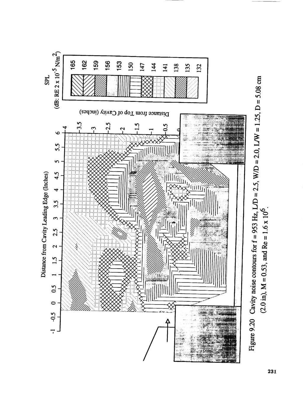
251 o,i 231

252 tt3 t-/ &i eq 1".'4 _ t.',"4 _ v._ ee_ e,q II C2 d ee_ o_ c:/ II d II t-,,-; II eq o II o II! m 232

253 ,9, eq O o. tt_ II cq II o" e,i II m 233