Advanced Calibration Topics - II

Transcription

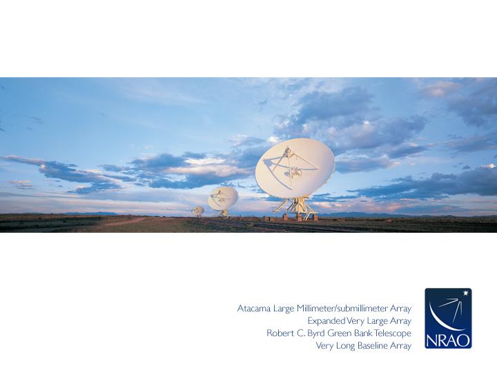
1 Advanced Calibration Topics - II Crystal Brogan (NRAO) Sixteenth Synthesis Imaging Workshop May 2018

2 Effect of Atmosphere on Phase 2

3 Mean Effect of Atmosphere on Phase Since the refractive index (n) of the atmosphere 1, an electromagnetic wave propagating through it will have a phase change (i.e. Snell s law) The phase change is related to the refractive index of the air, n, and the distance traveled, D, by For water vapor n µ f e = (2p/l) n D W DT atm W = precipitable water vapor (PWV) column T atm = Temperature of atmosphere so f e» 12.6p W l for T atm = 270 K Refraction causes: - Pointing off-sets, Δθ 2.5x10-4 x tan(i) elevation 45 o typical offset~1 - Delay (time of arrival) off-sets ð These mean errors are generally removed by the online system 3

4 Atmospheric phase fluctuations Variations in the amount of precipitable water vapor (PWV) cause phase fluctuations, which are worse at shorter wavelengths (higher frequencies), and result in: Loss of coherence (loss of S/N) Radio seeing, typically 0.1-1² at 1 mm Anomalous pointing offsets Anomalous delay offsets You can observe in apparently excellent submm weather (in terms of transparency, i.e. low PWV) and still have terrible seeing i.e. phase stability. Patches of air with different water vapor content (and hence index of refraction) affect the incoming wave front differently. 4

5 Atmospheric phase fluctuations, continued Phase noise as function of baseline length log (RMS Phase Variations) Power law a Break typically a few hundred meters to a few kilometers Increasing Baseline Length Root phase structure function (Butler & Desai 1999) RMS phase fluctuations grow as a function of increasing baseline length until break when baseline length thickness of turbulent layer The position of the break and the maximum phase variation are weather and wavelength dependent RMS phase of fluctuations given by Kolmogorov turbulence theory f rms = K b a / l [deg] b = baseline length (km) a = 1/3 to 5/6 (thin atmosphere vs. thick atmosphere) l= wavelength (mm) K = constant (~100 for ALMA, 300 for JVLA) 5

6 Residual Phase and Decorrelation Q-band (7mm) VLA C-config. data from good day An average phase has been removed from absolute flux calibrator 3C286 Short baseline Long baseline Coherence = (vector average/true visibility amplitude) = ávñ/ V 0 Where, V = V 0 e if The effect of phase noise, f rms, on the measured visibility amplitude : ávñ = V 0 áe if ñ = V 0 e -f 2 rms /2 (Gaussian phase fluctuations) Example: if f rms = 1 radian (~60 deg), coherence = ávñ = 0.60V 0 (minutes) ðresidual phase on long baselines have larger excursions, than short baselines For these data, the residual rms phase (5-20 degrees) from applying an average phase solution produces a 7% error in the flux scale 6

7 22 GHz VLA observations of the calibrator Position offsets due to large scale structures that are correlated ð phase gradient across array All data: Reduction in peak flux (decorrelation) and smearing due to phase fluctuations over 30 min resolution of 0.1 (Max baseline 30 km) one-minute snapshots at t = 0 and t = 59 minutes Sidelobe pattern shows signature of antenna based phase errors ð small scale variations that are uncorrelated Corrections 30min: Corrections 30sec: No sign of phase fluctuations errors with correction timescale ~ 30 s ð Uncorrelated phase variations degrades and decorrelates image ð Correlated phase offsets = position shift 7

8 Phase Correction Techniques 8

9 Phase fluctuation correction methods Fast switching (Observing strategy) - used at the JVLA and ALMA for higher frequencies and longer baselines. Choose fast switching cycle time, t cyc, short enough to reduce Φ rms to an acceptable level. Calibrate in the normal way. Radiometer (Observing Strategy) - Monitor phase (via path length) with special dedicated receivers. Requires modeling the atmosphere. Used by ALMA. Self-calibration: Requires adequate antenna-based S/N Phase transfer (Band-2-Band; Observing Strategy): simultaneously observe low and high frequencies, and transfer scaled phase solutions from low to high frequency. Tricky, requires well characterized system due to differing electronics at the frequencies of interest. Currently being commissioned at ALMA. Paired array calibration (Observing Strategy): divide array into two separate arrays, one for observing the source, and another for observing a nearby calibrator. Will not remove fluctuations caused by electronic phase noise Can only work for arrays with large numbers of antennas (was used by CARMA) 9

10 Fast Switching (an observing strategy) Fast switching phase calibration will stop tropospheric phase fluctuations on baselines longer than an effective baseline length of: b eff = V a t cyc 2000! t cyc (s) = 200 φ rms(deg)λ(mm) $ # & " K % b eff : effective baseline length in km V a : velocity of the winds aloft in m/s (~10 m/s at JVLA) t cyc : cycle time in seconds (~120 sec) Cycle times shorter than the baseline crossing time of the troposphere are needed. For example, substituting into the phase rms Eq on slide 5 with α = 0.7 and Va=10m/s (typical for JVLA site) yields: 1.42 K = constant (~100 for ALMA, ~300 for VLA) Note that a 90 degree phase rms will easily wipe out a source. JVLA Phase monitor: 10

11 Radiometers (an observing strategy): Radiometry: measure fluctuations in T B atm with a radiometer, use these to derive changes in water vapor column (w) and convert this into a phase correction using f e» 12.6p W l W=precipitable water vapor (PWV) column 22 GHz 183 GHz (Bremer et al. 1997) Monitor: 22 GHz H 2 O line (CARMA, JVLA) 183 GHz H 2 O line (CSO-JCMT, SMA) total power (IRAM) Correct: 183 GHz H 2 O line (ALMA) 11

12 ALMA s particular need for WVR correction: Observations at 300 microns (Band 10) require a path error less than 25 microns to keep the phase fluctuations < 30 degrees ALMA site testing suggests that the median path fluctuation due to the atmosphere is ~200 microns on 300 m baselines (compared to max of 15 km) These fluctuations increase with baseline length (up to several km) according to Kolmogorov with a power of about 0.6 for the ALMA site Changes on timescales as small as the Antenna diameter/wind speed are possible = 1 sec ALMA WVRs monitor changes in water line brightness: 183 GHz H 2 O line and psuedocontinuum There are 4 channels flanking the peak of the 183 GHz water line Data taken every second Installed on all the 12m antennas Matching data from opposite sides are averaged The four channels allow flexibility for avoiding saturation 12

13 Modeling the Path Change Challenge: Convert changes in 183 GHz brightness to changes in path length Implementation offline: wvrgcal 3 unknowns: PWV, temperature, pressure (in water vapor layer) in a simple plane parallel, thin layer model HITRAN and radiative transfer is used to derive the line shape, opacity and hence brightness temperature T B (H2O) as a function of frequency The observed spectrum is then compared to the model predictions for a range of reasonable values of PWV, Temperature, and pressure After dropping smaller terms: D(path) = D(PWV) * 1741/T(H2O layer) The path change is converted to phase for the mean frequency of each science spectral window For a more complete description ALMA Memo 587 PWV from 0.6 to 1.3mm Temperature from 230 to 300 K Pressure from 400 to 750 mbar 13

14 ALMA WVR Correction - Examples Band 6 (230 GHz) Compact config Band 7 (340 GHz) Extended config Raw phase & WVR corrected phase 14

15 Self-Calibration: Motivation JVLA and ALMA have impressive sensitivity! But what you achieve is often limited by residual calibration errors Many objects will have enough Signal-to-Noise (S/N) so they can be used to better calibrate themselves to obtain a more accurate image. This is called self-calibration and it really works, if you are careful! Sometimes, the increase in effective sensitivity may be an order of magnitude. It is not a circular trick to produce the image that you want. It works because the number of baselines is much larger than the number of antennas so that an approximate source image does not stop you from determining a better temporal gain calibration which leads to a better source image. 15

16 Data Corruption Types The true visibility is corrupted by many effects: Atmospheric attenuation Radio seeing Variable pointing offsets Variable delay offsets Electronic gain changes Electronic delay changes Electronic phase changes Radiometer noise Correlator mal-functions Most Interference signals Antenna-based baseline 16

17 Antenna-based Calibration- I The most important corruptions are associated with antennas Basic Calibration Equation Factorable (antenna-based) complex gains Non-factorable complex gains (not Antenna based and typically small) True Visibility Additive offset (not antenna based and typically small) Thermal noise Can be reduced to (approximately) 17

18 Antenna-based Calibration-II For N antennas, [(N-1)*N]/2 visibilities are measured, but only N amplitude and (N-1) phase gains fully describe the complete Antenna-based calibration. This redundancy is used for antenna gain calibration Basic gain (phase and amplitude) calibration involves observing unresolved (point like) calibrators of known position with visibility M i,j (t k, n) Determine gain corrections, g i, that minimizes S k for each time stamp t k where S k = k i j i,j w i,j g i (t k )g j (t k )V o i,j(t k ) M i,j (t k ) 2 Data Weights Complex Gains Complex Visibilities Fourier transform of model image The solution interval, t k, is the data averaging time used to obtain the values of g i, (i.e. solint= int or inf ). The apriori weight of each data point is w i,j. This IS a form of Self-calibration, only we assume a Model (Mij) that has constant amplitude and zero phase, i.e. a point source The transfer of these solutions to another position on the sky at a different time (i.e. your science target) will be imperfect, but the same redundancy can be used with a model image for Self-calibration 18

19 Sensitivities for Self-Calibration-I For phase only self-cal: Need to detect the target in a solution time (solint self ) < the time for significant phase variations with only the baselines to a single antenna with a S/N self 3. For 25 antennas, S/N Self > 3 will lead to < 15 deg error. Make an initial image, cleaning it conservatively Measure rms in emission free region of image rms Ant = rms x N 3 where N is # of antennas rms self = rms Ant x Time_on_source/solint self Measure Peak flux density = Signal If S/N self = Peak/rms Self >3 try phase only self-cal Rule of thumb: For an array with ~25 antennas, if S/N in image >20 its worth trying phase-only self-cal CAVEAT 1: If dominated by extended emission, estimate what the flux will be on the longer baselines (by plotting the uv-data) instead of the image If the majority of the baselines in the array cannot "see" the majority of emission in the target field (i.e. emission is resolved out) at a S/N of about 3, the self-cal will fail in extreme cases (though bootstrapping from short to longer baselines is possible, it can be tricky). CAVEAT 2: If severely dynamic range limited (poor uv-coverage), it can also be helpful to estimate the rms noise from uv-plots 19

20 Sensitivities for Self-Calibration-II For amplitude self-cal: Need to detect the target with only the baselines to a single antenna with a S/N self 10, in a solution time (solint self ) < the time for significant amplitude variations. For 25 antennas, an antenna based S/N > 10 will lead to a 10% amplitude error. Amplitude corrections are more subject to deficiencies in the model image, check results carefully! For example, if clean model is missing significant flux compared to uv-data, give uvrange for amplitude solution that excludes short baselines Additional S/N for self-cal can be obtained by: Increase solint (solution interval) Errors that are directional, rather than time dependent can yield surprising improvement even if the solint spans the whole observation = antenna position (aka baseline) errors are a good example gaintype= T to average polarizations Phase differences between polarizations are generally well calibrated Combine = spw to average spw s (assumes prior removal of spw to spw offsets) Caveat: If source spectral index/morphology changes significantly across the band, do not combine spws, especially for amplitude self-cal unless you use mtmfs Combine = fields to average fields in a mosaic (use with caution, only fields with strong signal) 20

21 Self-calibration Example: ALMA SV Data for IRAS16293 Band 6 (Ia) Step 1 Determine basic setup of data: 2 pointing mosaic Integration = sec; subscans ~ 30sec Scan= 11min 30s (split between two fields) Step 2 What is the expected rms noise? Use actual final total time and # of antennas on science target(s) from this stage and sensitivity calculator. Be sure to include the actual average weather conditions for the observations in question and the bandwidth you plan to make the image from 54 min per field with 16 antennas and average Tsys ~ 80 K, 9.67 MHz BW; rms= 1 mjy/beam Inner part of mosaic will be about 1.6 x better due to overlap of mosaic pointings ALMA mosaic: alternates fields in subscan this picture = 1 scan EVLA mosaic: alternates fields in scans Subscans are transparent to CASA (and AIPS) 21

22 Self-calibration Example: ALMA SV Data for IRAS16293 Band 6 (Ib) Step 3 What does the amplitude vs uv-distance of your source look like? Does it have large scale structure? i.e. increasing flux on short baselines. What is the flux density on short baselines? Keep this 4 Jy peak in mind while cleaning. What is the total cleaned flux you are achieving? 22

23 Self-calibration Example: ALMA SV Data for IRAS16293 Band 6 (II) Step 4 What is the S/N in a conservatively cleaned image? What is this conservative of which you speak Rms~ 15 mjy/beam; Peak ~ 1 Jy/beam è S/N ~ 67 Rms > expected and S/N > 20 è self-cal! Residual after 200 iterations Stop clean, and get rms and peak from image, avoiding negative bowls and emission Clean boxes only around emission you are SURE are real at this stage 23

24 Self-calibration Example: ALMA SV Data for IRAS16293 Band 6 (III) Step 5: Decide on an time interval for initial phase-only self-cal A good choice is often the scan length (in this case about 5 minutes per field) Exercise for reader: from page 31 show that S/N self ~ 5.4 In CASA you can just set solint= inf (i.e. infinity) and as long as combine scan AND field you will get one solution per scan, per field. Use T solution to combine polarizations What to look for: Lot of failed solutions on most antennas? if so, go back and try to increase S/N of solution = more averaging of some kind Do the phases appear smoothly varying with time (as opposed to noise like) 24

25 Self-calibration Example: ALMA SV Data for IRAS16293 Band 6 (IV) Step 6: Apply solutions and re-clean Incorporate more emission into clean box if it looks real Stop when residuals become noise-like but still be a bit conservative, ESPESCIALLY for weak features that you are very interested in You cannot get rid of real emission by not boxing it You can create features by boxing noise Step 7: Compare Original clean image with 1 st phase-only self-cal image Original: Rms~ 15 mjy/beam; Peak ~ 1 Jy/beam è S/N ~ 67 1 st phase-only: Rms~ 6 mjy/beam; Peak ~ 1.25 Jy/beam è S/N ~ 208 Did it improve? If, yes, continue. If no, something has gone wrong or you need a shorter solint to make a difference, go back to Step 4 or stop. Original 1 st phase cal 25

26 Self-calibration Example: ALMA SV Data for IRAS16293 Band 6 (V) Step 8:Try shorter solint for 2 nd phase-only self-cal In this case we ll try the subscan length of 30sec It is best NOT to apply the 1 st self-cal while solving for the 2 nd. i.e. incremental tables can be easier to interpret but you can also build in errors in first model by doing this What to look for: Still smoothly varying? If this looks noisy, go back and stick with longer solint solution IF this improves things a lot, could try going to even shorter solint 26

27 Self-calibration Example: ALMA SV Data for IRAS16293 Band 6 (VI) Step 9: Apply solutions and re-clean Incorporate more emission into clean box if it looks real Stop when residuals become noise-like but still be a bit conservative, ESPECIALLY for weak features that you are very interested in You cannot get rid of real emission by not boxing it You can create features by boxing noise Step 10: Compare 1 st 1 st phase-only: and 2 nd phase-only self-cal images Rms~ 6 mjy/beam; Peak ~ 1.25 Jy/beam è S/N ~ nd phase-only: Rms~ 5.6 mjy/beam; Peak ~ 1.30 Jy/beam è S/N ~ 228 Did it improve? Not much, so going to shorter solint probably won t either, so we ll try an amplitude self-cal next 1 st phase cal 2 nd phase cal 27

28 Self-calibration Example: ALMA SV Data for IRAS16293 Band 6 (VII) Step 11:Try amplitude self-cal Amplitude tends to vary more slowly than phase. It s also less constrained, so solints are typically longer. Lets try two scans worth or 23 minutes Essential to apply the best phase only self-cal before solving for amplitude. Also a good idea to use mode= ap rather than just a to check that residual phase solutions are close to zero. Again make sure mostly good solutions, and a smoothly varying pattern. Scale +/- 10 degrees Scale 0.8 to 1.0 Residual phase Amplitude 28

29 Self-calibration Example: ALMA SV Data for IRAS16293 Band 6 (VIII) Step 12: Apply solutions Apply both 2 nd phase and amp cal tables Inspect uv-plot of corrected data to Check for any new outliers, if so flag and go back to Step 9. Make sure model is good match to data. Confirm that flux hasn t decreased significantly after applying solutions Original Image Model (total cleaned flux = 3.4 Jy) Amp & Phase applied 29

30 Self-calibration Example: ALMA SV Data for IRAS16293 Band 6 (IX) Step 13: Re-clean Incorporate more emission into clean box Stop when residuals become noise-like clean everything you think is real Step 14: Compare 2 nd phase-only and amp+phase self-cal images 2 nd phase-only: Rms~ 5.6 mjy/beam; Peak ~ 1.30 Jy/beam è S/N ~ 228 Amp & Phase: Rms~4.6 mjy/beam; Peak~1.30 Jy/beam è S/N ~283 Did it improve? è Done! Final: S/N=67 vs 283! But not as good as theoretical = dynamic range limit 2 nd Original phase cal Amp & Phase cal 30

31 Self-Calibration example 2: JVLA Water Masers (I) uv-spectrum after standard calibrator-based calibration for bandpass and antenna gains There are 16 spectral windows, 8 each in two basebands (colors in the plot) Some colors overlap because the basebands were offset in frequency by ½ the width of an spw in order to get good sensitivity across whole range. The continuum of this source is weak. How do you self-cal this? In general DATA CHANNEL NUMBER IMAGE CHANNEL NUMBER due to Doppler Shift, also LSB windows will have negative channel width, i.e. data and image channel numbers going in opposite directions (as of CASA 5.1) Suggest running CVEL using the rest frequency of the line at the same velocity resolution that you want for the final cube this will give you a uv-dataset with the same channelization as the cube you want DATA CHANNEL NUMBER = IMAGE CHANNEL NUMBER 31

32 Self-Calibration example 2: JVLA Water Masers (III) Need to know the SPWs and the CHANNELs with strong emission in the model: plotms of the MODEL (no CVEL, so data channels image channels) with locate can help From the locate we find a strong set of channels in spw=3 channels 12~22 spw=12 channels 76~86 We use these channels in the self-calibration. It is very important not to include channels without signal in the clean model! 32

33 Self-Calibration example 2: JVLA Water Masers (III) Final self-calibrated spectrum Peak amplitude increased from 350 Jy/beam to 500 Jy/beam (a 40% increase) due to correction of decorrelation One remaining trickiness: calibration solutions are only for spw=3 and 12. The spwmap parameter can be used to map calibration from one spectral window to another in applycal. There must be an entry for all spws (16 in this case): spwmap=[3,3,3,3,3,3,3,3,12,12,12,12,12,12,12,12] In other words apply the spw=3 calibration to the 8 spectral windows in the lower baseband and the calibration from spw=12 to the 8 spws in the upper baseband Beyond this everything is the same as previous example. 33

34 Summary Spatial and temporal variations in the amount of precipital water vapor in the troposphere cause phase fluctuations but there are a wide range of options for corrections: observing techniques and post-processing Fast switching WVRs Self-calibration Self-calibration is not so hard and can make a big difference Make sure your model is a good representation of the data Make sure the data you put into solver, is a good match to the model If you are lacking a little in S/N try one of the S/N increase techniques If you really don t have enough S/N don t keep what you try! For more examples, tips, tricks, and advice see 34

35 Calibration Sensitivities Effects (N=25) S/N Ant Amp error Phase error S/N base S/N image 0 100% 180 d % 15.0 d % 9.7 d % 5.7 d % 2.3 d % 0.6 d d Ant phase error must be smaller than expected instrumental and tropospheric phase error which is often deg d Ant amp error must be smaller than expected instrumental and absorption amplitude errors, usually < 5% 35