Section 3: Functions of several variables.

Transcription

1 Section 3: Functions of several variables. Compiled by Chris Tisdell S1: Motivation S2: Function of two variables S3: Visualising and sketching S4: Limits and continuity S5: Partial differentiation S6: Chain rule + differentiability S7: Gradient + directional derivative S8: Linear approximation S9: Error estimation S10: Taylor series Images from Thomas calculus by Thomas, Wier, Hass & Giordano, 2008, Pearson Education, Inc. 1

2 S1: Motivation. Phenomena of a complex nature usually depend on more than one variable. Applications matter! The amount of power P (in watts) available to a wind turbine can be summarised by the equation P = 1 ( ) 49 (πr 2 )v where r = diameter of turbine blades exposed to the wind (m) v = wind speed in m/sec 49/40 is the density of dry air at 15 deg C at sea level (kg/m 3 ). See that the power P depends on two variables, r and v, that is, P = f(r, v). 2

3 You have already studied functions of 1 variable at school. You developed curve sketching skills and a knowledge of calculus for functions of the type y = f(x). In this section we extend these ideas to functions of many variables. In particular, we will learn the idea of a derivative for these more complicated functions. Such ideas give us the power to more accurately model and understand complex phenomena like that of the previous example. 3

4 S2: Functions of two variables. We will consider functions of the type z = f(x, y), (x, y) U where U R 2 is the domain of f and f is real valued. We write f : U R 2 R. Examples of f and U: f(x, y) = x cos y + xy sin x, U = R 2 1 f(x, y) = 2x y, U = {(x, y) R2 : y 2x} f(x, y) = x + y, U = {(x, y) R 2 : x + y 0}. More simply: 4

5 S3: Visualising & sketching. As a first step to understanding functions of two variables, we now develop some methods for visualising and sketching their graphs. 5

6 Graphs for functions of 2 variables will be surfaces in R 3. 6

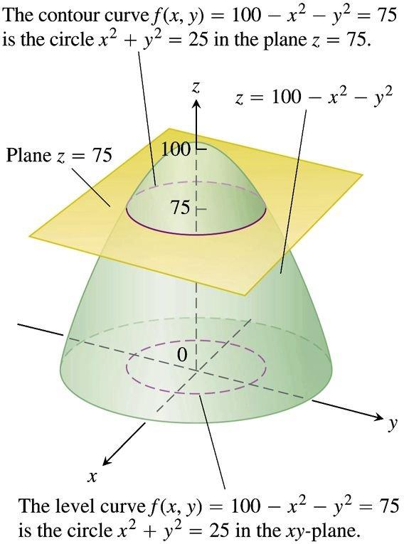
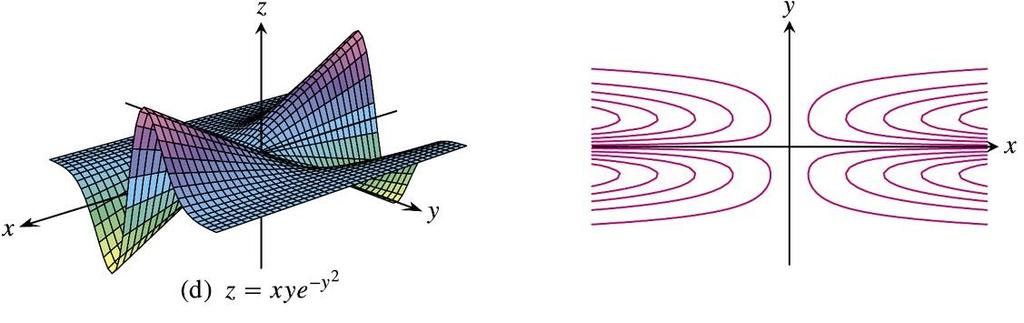
7 For a given function f, we can determine the nature of its graph by examining how the surface intersects with various planes and then build the surface from these curves. Horizontal planes: Contour curves & level curves. A contour curve of f is the curve of intersection between the surface z = f(x, y) and a horizontal plane z = c, c = constant. For simple cases, a contour curve can be easily drawn in R 3 and observe that this curve also lies in the plane z = c. If we sketch our contour curve in the XY -plane, then we obtain what is known as a level curve of f. 7

8 8

9 9

10 10

11 Ex: Sketch the surface z = x 2 + y 2 /9. 11

12 Ex: Sketch the level curves associated with f(x, y) = y 2 x 2. There are many other important surfaces, which we list a little later. 12

13 Applications matter! The idea of contour curves is similar to that used to prepare contour maps where lines are drawn to represent constant altitudes. Walking along a line would mean walking on a level path. 13

14 14

15 Level surface 15

16 Common surfaces + their properties. Ellipsoid x 2 /a 2 + y 2 /b 2 + z 2 /c 2 = 1 16

17 Paraboloid z/c = x 2 /a 2 + y 2 /b 2 17

18 Hyperboloid (1 sheet) x 2 /a 2 + y 2 /b 2 z 2 /c 2 = 1 18

19 Hyperboloid (2 sheets) z 2 /c 2 x 2 /a 2 y 2 /b 2 = 1 19

20 Elliptic Cone x 2 /a 2 + y 2 /b 2 = z 2 /c 2 20

21 Hyperbolic Paraboloid y 2 /b 2 x 2 /a 2 = z/c 21

22 Review your understanding: 1) Generally speaking, what is the form of the graph of f(x, y)? 2) T/F: If the level curves of a function f(x, y) are concentric circles, then the graph is a cone. 3) T/F: For z = f(x, y) the z value measures how far each point on the surface lies above or below the point (x, y) in the XY plane. 22

23 S4: Limits and continuity. For functions of two variables, the idea of a limit is more profound due to the more general domains of these functions. If R is the domain of f then we can approach (x 0, y 0 ) from many different directions (not just from 2 directions as in first year studies). 23

24 Roughly speaking our definition says that the distance between f(x, y) and L becomes (arbitrarily) small when the distance between (x, y) and (x 0, y 0 ) is sufficiently small (but not zero). Above we always assume that (x, y) is in the domain of f so that limits of boundary points may be included. 24

25 25

26 Ex: If then calculate f(x, y) := x2 + y x + y lim f(x, y). (x,y) (1,2) 26

27 Ex: If f(x, y) := x 2 + y then formally prove f(x, y) 3 as (x, y) (0, 0). 27

28 Ex: If f(x, y) := y x then formally prove f(x, y) 0 as (x, y) (0, 0). 28

29 Ex: Show that f(x, y) := has no limit as (x, y) (0, 0). 3x3 y x 4 + y 4 29

30 Ex: If f(x, y) := 2xy/(2 + sin x) then show f is continuous at (0, 0). Hint: Use Young s inequality 2ab a 2 + b 2. 30

31 Ex: Show that f(x, y) = is not continuous at (0, 0). 2x 2 x 2 +y 2, (x, y) (0, 0); 0, (x, y) = (0, 0) 31

32 Ex: By switching to polar co ordinates x = r cos θ, y = r sin θ and using the fact that if f has a limit L then show that lim f(x, y) = lim f(r cos θ, r sin θ) = L (x,y) (0,0) r 0 f(x, y) = is continuous at (0, 0). x 3 x 2 +y2, (x, y) (0, 0); 0, (x, y) = (0, 0) 32

33 S5: Partial differentiation. We know from elementary calculus that the idea of a derivative is very helpful in the mathematical analysis of applied problems. We now extend this concept to functions of two variables. For a function of two variables f = f(x, y), the basic idea is to determine the rate of of change in f with respect to one variable, while the other variable is held fixed. 33

34 Essentially f/ x is just the derivative of f with respect to x, keeping the y variable fixed. 34

35 35

36 Essentially f/ y is just the derivative of f with respect to y, keeping the x variable fixed. 36

37 37

38 Ex: If f(x, y) := x 3 y + y 2 then calculate f/ x and f/ y. 38

39 39

40 Ex: If f(x, y) := sin(xy) then calculate: f x (0, π); f y (2, 0). 40

41 Ex: For f(x, y) := x 2/3 y 1/3 show f x = 0 at (0, 0). 41

42 Product and quotient rules for partial differentiation are defined in the natural way: x (uv) = u xv + v x u x ( ) u v = u xv v x u v 2 y (uv) = u yv + v y u y ( ) u v = u yv v y u v 2. 42

43 43

44 Ex: The plane x = 1 intersects the paraboloid z = x 2 + y 2 in a parabola as shown in the following diagram. Calculate the slope of that tangent line to the parabola at the point (1,2,5). 44

45 Partial derivatives + continuity Continuity of partial derivatives of f implies continuity of f (and also implies what is known as differentiability of f). 45

46 Higher derivatives: We define and denote the second order partial derivatives of f as follows: 46

47 See that there are four partial second order derivatives and two of them are mixed. The order of differentiation is, in general, important (but see below for an important exception). 47

48 Ex: If f(x, y) = 1+x 5 +y 3 then compute all four 2nd order partial derivatives. What do you notice about the mixed derivatives? 48

49 Ex: Consider the function f(x, y) = xy + x + y. (a) Calculate f xx and f yy. (b) Use (a) to show f xx xf yy = 0 (1) 49

50 Applications matter! Equation (1) is known as a partial differential equation (PDE). A PDE involves: partial derivatives of an unknown function and an equals sign. The PDE (1) is a special equation known as the Euler Tricomi equation, which is used to desribe transonic fluid (air) flow over aircraft. Part (b) from the previous example says that f(x, y) = xy + x + y is a solution to the Euler Tricomi equation. 50

51 S6: Differentiability & chain rules. The goal of this section is to suitably define the concept of differentiability of functions f = f(x, y) and explore some of the interesting consequences and applications including the chain rule. In first year you learnt that a function f = f(x) is differentiable at a point x = x 0 if f(x) f(x lim 0 ), exists (2) x x 0 x x 0 and we denote the value of this limit by f (x 0 ). 51

52 In particular, when we say that a function f = f(x) is differentiable at x 0 (an interior point of dom f), we mean that there is a (unique) affine function A that suitably approximates f near x 0. In the case f = f(x), the affine function is of the form A(x) = ax + b, where a and b are particular constants. It turns out that the graph of A is just the tangent line to f at x 0 and so A(x) = f(x 0 ) + f (x 0 )(x x 0 ) = f(x 0 ) + L(x x 0 ) so that: a = f (x 0 ); and b = f(x 0 ) f (x 0 )x 0. Above, L is the linear function that represents multiplication by a = f (x 0 ). 52

53 What do we mean by A suitably approximates f near x 0? We mean: (i) f(x 0 ) = A(x 0 ); and (ii) f(x) A(x) approaches 0 faster than x approaches x 0, that is, f(x) A(x) lim = 0, ie x x 0 x x 0 f(x) f(x lim 0 ) L(x x 0 ) = 0 (3) x x 0 x x 0 which may be equivalently written as: there is a function ε(x) such that f(x) = f(x 0 ) + L(x x 0 ) + (x x 0 )ε(x x 0 ), lim x 0 ε(x) = 0. and The above kind of approximation is known as linear or first degree approximation. 53

54 The concept of differentiability is more subtle in the case f = f(x, y) but we can build a useful definition very naturally from the previous discussion. When we say that a function f = f(x, y) is differentiable at (x 0, y 0 ) (an interior point of dom f), we mean that there is a (unique) affine function A = A(x, y) that suitably approximates f near (x 0, y 0 ) in the sense that f(x, y) A(x, y) goes to zero faster than (x, y) goes to (x 0, y 0 ). That is, there is a linear function L such that lim (x,y) (x 0,y 0 ) f(x, y) f(x 0, y 0 ) L(x x 0, y y 0 ) (x x 0 ) 2 + (y y 0 ) 2 = 0. The above may be equivalently written as: there is a function ε = ε(x, y) such that f(x, y) = f(x 0, y 0 ) + L(x x 0, y y 0 ) + ε(x x 0, y y 0 ) (x x 0 ) 2 + (y y 0 ) 2, and lim ε(x, y) = 0. (x,y) (0,0) 54

55 Independent learning ex: What do you think is the particular form of A(x, y) or L(x, y) and what might the graph of A represent? Indep. learning ex: Show that for f = f(x) the definition of differentiability (3) is equivalent to our first year definition of differentiability (2) (with L representing multiplication by a = f (x 0 )). Many important functions of two (or more) variables satisfy the following. Thus, functions such as polynomials are always differentiable. 55

56 Chain rules. We have discussed various rules for partial differentiation, like product and quotient rules. What other concepts can we apply to help us to find partial derivatives?? Remember the chain rule for functions of one variable? For functions of more than one variable, the chain rule takes a more profound form. The easiest way of remembering various chain rules is through simple diagrams. 56

57 Case I: w = f(x) with x = g(r, s) 57

58 Ex: If w = f(r 2 + s 2 ), with f differentiable, then show that f satisfies the partial differential equation (PDE) sf r rf s = 0. Indep. learning ex: If a is a constant and f and g are diff able then show z = f(x + at) + g(x at) satisfies the wave equation z tt = a 2 z xx. 58

59 Case II: w = f(x, y) with x = x(t), y = y(t) 59

60 Ex: If f(x, y) = xy 2 with x = cos t and y = sin t then use the chain rule to find df/dt. 60

61 Applications matter! Ex: The pressure P (in kilopascals); volume V (litres) and temperature T (degrees K) of a mole of an ideal gas are related by the equation P = 8.31T/V. Find the rate at which the pressure is changing wrt time when: T = 300; dt/dt = 0.1; V = 100; dv/dt = 0.2. We calculate dp/dt and evaluate it at the above instant. 61

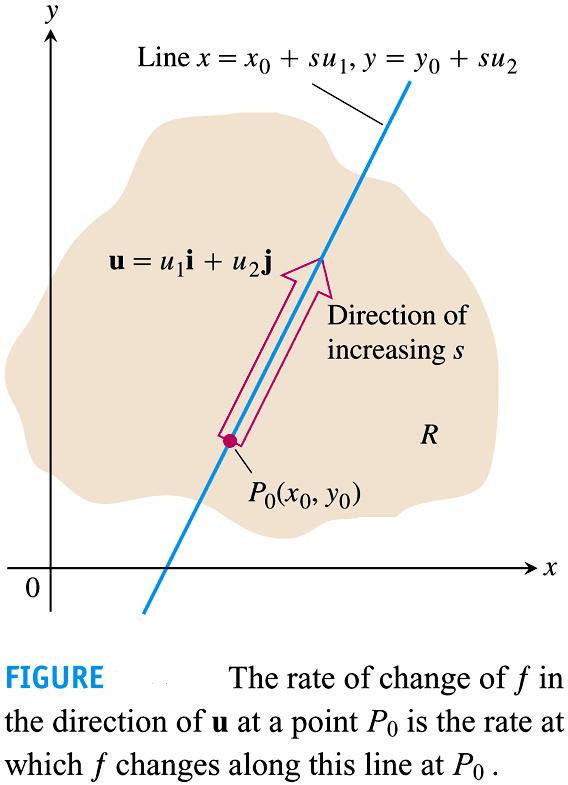
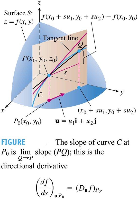
62 Case III: w = f(x, y) with x = g(r, s), y = h(r, s) 62

63 Ex: Let f have continuous partial derivatives. Show that z = f(u v, v u) satisfies the PDE z u + z v = 0. 63

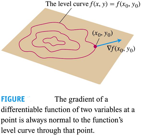
64 Case IV: w = f(x, y, z) with x = x(t), y = y(t), z = z(t) 64

65 65

66 66

67 Case V: w = f(x, y, z) with x = g(r, s), y = h(r, s), z = k(r, s) 67

68 68

69 Applications matter! Advection, in mechanical and chemical engineering, is a transport mechanism of a substance or a conserved property with a moving fluid. The advection PDE is a u x + u t = 0 (4) where a is a constant and u(x, t) is the unknown function. Use the chain rule to show that a solution to (4) is of the form u(x, t) = f(x at) where f is a differentiable function. Perhaps the best image to have in mind is the transport of salt dumped in a river. If the river is originally fresh water and is flowing quickly, the predominant form of transport of the salt in the water will be advective, as the water flow itself would transport the salt. Above, u(x, t) would represent the concentration of salt at position x at time t. 69

70 S7: Gradient & directional derivative. We now generalise our ability to determine the rate of change of f to any direction. The ideas are extensions of partial derivatives. 70

71 71

72 The equation z = f(x, y) represents a surface S in space (see following diagram). If z 0 = f(x 0, y 0 ) then the point P (x 0, y 0, z 0 ) lies on S. The vertical plane that passes through P and P 0 (x 0, y 0 ) that is parallel to û intersects S in a curve C. The rate of change of f in the direction of û is the slope of the tangent line to C at P. 72

73 73

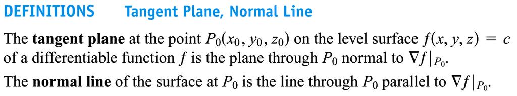
74 There is a more efficient formula for the directional derivative than the one we have seen. The new formula involves f, the gradient of f, which we now explore more deeply. Ex: If f(x, y) := x 3 + y then calculate f and f(1, 2). 74

75 75

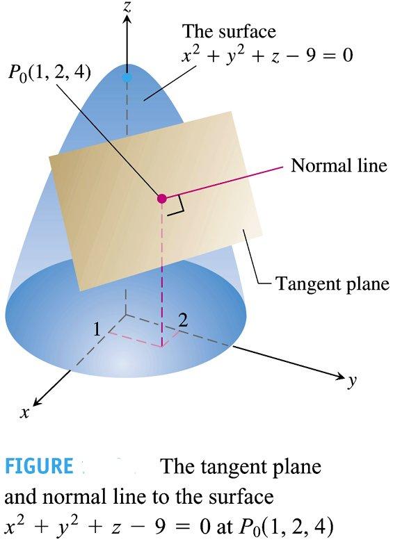
76 If θ is the angle between the vectors û and f then the formula Dûf = f û = f û cos θ = f cos θ reveals the following properties. Why do we use a unit vector û in our definition of directional derivative? In this case, Dûf is the rate of change of f per unit change in the direction of û. 76

77 77

78 Ex: At the point (1, 1), determine the directions in which f(x, y) := x 2 /2 + y 2 /2: increases most rapidly; decreases most rapidly; has zero change. 78

79 Applications matter! Experiments show that if a piece of material is heated on one side and cooled on another, then heat flows in the direction of maximum decrease of temperature. That is, heat flows from hot regions toward cold regions. If the temperature T = T (x, y) is given by T = x 3 3xy 2 then determine the direction of maximum decrease of temperature at the point P (1, 2). 79

80 Similarly, for f(x, y, z) we define f := f x i + f y j + f z k and verbally refer to f as grad f. Note that f is vector valued (but f is not)! Ex: If f(x, y, z) := x 3 +y+z 2 then calculate f and f(1, 2, 3). 80

81 Ex: Calculate the derivative of f(x, y, z) := x 3 xy 2 z at P 0 (1, 1, 0) in the dir n of v = 2i 3j + 6k. 81

82 Chain rule involving the gradient: d dt [f(r(t)] = f(r(t)) r (t). 82

83 Applications matter! In the following contour map of the West Point area in New York, see that the tributary streams to the Hudson flow perpendicular to the contours. Explain and justify! 83

84 Tangent plane, normal line and other applications of f. 84

85 85

86 Ex: Calculate the tangent plane and the normal line to the surface x 2 + y 2 + z = 9 at the point P 0 (1, 2, 4). 86

87 87

88 Let the the graph of z = f(x, y) represent the surface of a mountain lying above the XY plane. The angle of inclination ψ, which measures the steepness of the terrain in the direction û is tan ψ = slope of tangent in dir n û = Dûf. 88

89 Check your understanding. Ex: T/F: The expression ( f) is well defined. Ex: T/F: The expression f is well defined. Ex: T/F: There is a f(x, y) such that f = 5. Ex: Express f x in terms of Dûf for some û. Ex: If f is, loosely speaking, some sort of derivative of f, then what is the opposite operation that cancels the? Ex: T/F: Dûf is the scalar component of f in the direction of û Ex: T/F: (f n ) = nf n 1 f. 89

90 S8: Linear approximation. Geometrically, z = L(x, y) is the tangent plane to the surface z = f(x, y) at the point (x 0, y 0 ). If f is smooth enough then the tangent plane will provide a good approximation to f for points near to (x 0, y 0 ). 90

91 By smooth, we mean the surface has no corners, sharp peaks or folds. 91

92 Graph of the error between e x sin y and its tangent plane at (0,0). 92

93 The above concept roughly says that the polynomial L(x, y) gives a first order approximation to f(x, y) near the point (x 0, y 0 ) in the sense that: L(x 0, y 0 ) = f(x 0, y 0 ) (ie, the two surfaces touch at the point (x 0, y 0 )) lim (x,y) (x 0,y 0 ) (ie, the error is negligible when compared to f(x, y) L(x, y) (x x 0 ) 2 + (y y 0 ) 2 = 0 (x x 0 ) 2 + (y y 0 ) 2.) 93

94 S9: Error estimation. Using the tangent plane as an approximation to f near the point (x 0, y 0 ) we obtain f(x 0 + x, y 0 + y) (5) f(x 0, y 0 ) + f x (x 0, y 0 ) x + f y (x 0, y 0 ) y for small x and y. The above concept has important consequences in error estimation. When taking measurements (say, some physical dimensions), errors in the measurements are a fact of life. We now look at the effects of small changes in quantities and error estimation. 94

95 We define f := f(x 0 + x, y 0 + y) f(x 0, y 0 ) as the increment in f. Rearranging (5) we obtain f f x (x 0, y 0 ) x + f y (x 0, y 0 ) y. (6) If we take absolute values in (6) and use the triangle inequality then we obtain f f x (x 0, y 0 ) x + f y (x 0, y 0 ) y. (7) As a general guide: (6) is useful for approximating errors; while (7) is useful for estimating maximum errors. 95

96 Ex: The frequency f on a LC circuit is given by f(x, y) = x 1/2 y 1/2 2π where x is the inductance and y is the capacitance. If x is decreased by 1.5% and y is decreased by 0.5% then find the approximate percentage change in f. We use (6). For our problem: x = 1.5% of x = 0.015x and y = 0.5% of y = 0.005y. Also Thus (6) gives f x = x 3/2 y 1/2, 4π f y = x 1/2 y 3/2. 4π 96

97 f x 3 2y 1 2 ( 0.015x) + x 1 2y 3 2 ( 0.005y) 4π 4π = x 1 2y 1 2 (0.015) + x 1 2y 1 2 (0.005) [ 2π 2 2π = ] f 2 2 = 0.01f. The approximate % change in f is: f f = 1%. 97

98 Ex: Consider a cylinder with base radius r and height h measured (resp.) to be 5 cm and 12 cm, both calculated to nearest mm. What is the expectation for the maximum % error in calculating the volume? 98

99 The differentials dx and dy are independent variables and so they can be assigned any values. Sometimes we take dx = x = x x 0, dy = y = y y 0. We then have the following definition of the total differential of f: 99

100 Applications matter! A manufacturer produces cylindrical storage tanks with height 25m and radius 5m. As a quality control engineer hired by the company, perform an analysis on how sensitive the tanks volumes are to small variations in height and radius. Which measurement (height or radius) would you advise the company to pay particular attention to? Independent learning ex: What happens if the dimensions of the tanks are switched? Is your advice to the company the same? 100

101 S10: Taylor polynomials and Taylor series. Taylor polynomials and series for f(x). In first year you discovered Taylor polynomials and Taylor series. In particular, the aim was to develop a method for representing a (differentiable) function f(x) as an (infinite) sum of powers of x. The main thought process behind the method is that powers of x are easy to evaluate, differentiate and integrate, so by rewriting complicated functions as sums of powers of x we can greatly simplify our analysis. 101

102 102

103 Colin Maclaurin was a professor of mathematics at Edinburgh university. Newton was so impressed by Maclaurin s work that he offered to pay part of Maclaurin s salary. 103

104 Common Maclaurin series are above. If we take a finite number of terms in our series, then we obtain Taylor and Maclaurin polynomials, which are useful for approximation of functions. 104

105 Taylor s Theorem. Taylor s theorem is an extension of the mean value theorem. 105

106 When applying Taylor s theorem, we frequently wish to hold a fixed and consider b as an independent variable. If we change b to x in Taylor s formula, then it is easier to use in these cases. We obtain: The above version of Taylor s theorem says that for all x I we have f(x) = P n (x) + R n (x). 106

107 Taylor polynomials + series for f(x, y) The Taylor series expansion T (x, y) of a function f(x, y) of two independent variables about a point (a, b) is T (x, y) := f(a, b) + f x (a, b)(x a) + f y (a, b)(y b)+ 1 2! [ fxx (a, b)(x a) 2 + 2f xy (a, b)(x a)(y b) + f yy (a, b)(y b) 2] + (higher order terms) 107

108 We will be interested in Taylor polynomials of first and second order, ie T 1 (x, y) := f(a, b) + f x (a, b)(x a) + f y (a, b)(y b) T 2 (x, y) := T 1 (x, y) + 1 2! [ fxx (a, b)(x a) 2 + 2f xy (a, b)(x a)(y b) + f yy (a, b)(y b) 2]. In particular, T 1 and T 2 will provide (respectively) first and second degree approximations to f(x, y) near (a, b) 108

109 Ex: Calculate the Taylor polynomial (up to and including quadratic terms) about (a, b) = (0, 0) for f(x, y) = e x sin y. 109

110 We can graph the difference between the f and its Taylor polynomial. > plot3d(sin(y)*exp(x)-(y + x*y), x = , y = ); See that near (a, b) = (0, 0) the difference is small, but as we wander away from (0, 0) the difference grows. 110

111 Ex: Calculate the Taylor polynomial (up to and including quadratic terms) about (a, b) = (0, 0) for f(x, y) = 1 1 x y. 111

112 Ex: Use the formula to calculate the Taylor polynomial (up to and including quadratic terms) about (a, b) = (1, 0) for f(x, y) = ln(x 2 + y 2 ). 112

113 Taylor s formula / theorem for f(x, y) 113

114 Under the conditions of Taylor s theorem, the n th order Taylor polynomial T n for f about (0, 0) closely approximates f to the n th degree near (0, 0) in the sense that: lim (x,y) (0,0) T n (0, 0) = f(0, 0), f(x, y) T n (x, y) ( x 2 + y 2 ) n = 0. Furthermore, T n is the only polynomial of n th degree that satisfies the above. 114

115 Ex. Calculate the first order Taylor polynomial to f(x, y) := e x+y about (0, 0) and prove that it is a first degree approximation to f near (0, 0). 115

116 Where does the Taylor polynomial for f(x, y) come from? Let F (t) := f(tu + a, tv + b) where u and v are held fixed. Let s calculate the 2nd order Taylor poly of F about t = 0. From the chain rule we have: and so F (t) = uf x (tu + a, tv + b) + vf y (tu + a, tv + b) F (0) = uf x (a, b) + vf y (a, b). Similarly, the chain rule yields: F (t) = u 2 f xx (tu + a, tv + b) +2uvf xy (tu + a, tv + b) + v 2 f yy (tu + a, tv + b) and so F (0) = u 2 f xx (a, b) + 2uvf xy (a, b) + v 2 f yy (a, b). 116

117 If we replace: u with (x a); and v with (y b) then our (2nd order) Taylor polynomial for F (t) about t = 0 is T 2 (0) := F (0) + F (0)t + F (0)t 2 /2! which, for t = 1, becomes T 2 (a, b) = f(a, b) + f x (a, b)(x a) + f y (a, b)(y b) + 1 [ fxx (a, b)(x a) 2 + 2f xy (a, b)(x a)(y b) 2! +f yy (a, b)(y b) 2]. 117

118 S11: Appendix. Maple: Maple s plot3d command is used for drawing graphs of surfaces in threedimensional space. The syntax and usage of the command is very similar to the plot command (which plots curves in the two-dimensional plane). As with the plot command, the basic syntax is plot3d(what,how); but both the what and the how can get quite complicated. The commands for plotting the following paraboloid are: > z:=3*x^2+y^2; z := 3x 2 + y 2 > plot3d(z, x=-2..2,y=-2..2); 118