Volume. AnCAD INCORPORATED Simply Faster. Visual Signal DAQ Express User Guide

Transcription

1 Volume 1 AnCAD INCORPORATED Simply Faster Visual Signal DAQ Express User Guide

2 A N C A D I N C. Visual Signal DAQ Express User Guide AnCAD Inc. No. 1 Baosheng Rd. 16 Floor Yonghe District, New Taipei City Taiwan Phone Fax

3 Table of Contents Chapter 1 Introduction to Interface... 4 Function List... 4 Notational Conventions Application User Interface Graphical User Interface Introduction To The Toolbar Network Window (Component Editor Window) Components / Module Compiling Area Component Editor Toolbar Operation Control Area Data Viewer Visualization Window Property Window Properties of a Diagram Properties of a Component Importing Your Data Chapter 2 Example Projects Your First Project Spectrum Analysis Setting Up and Analyzing a Fourier Transformation Chapter 3 Data Acquisition Quick Start Recording Audio with Computer Recording audio data in a set amount of time Recording audio data in real-time Using ADLINK Installing the UD-DASK Driver Connecting the device Recording data with device Recording signal data in a set amount of time Recording signal data in real-time Chapter 4 Function List Computing With Signal Flow Object Channel Channel Switch i

4 Data Selection Fill Null Value Input Switch Remove Channel Replace Value Resample Time Shift Filter FIR Filter Median Filter Moving Average Filter Notch Filter Mathematics Differential Integrate Math Mixer Multiplier Normalize Remove DC RMS Time-Frequency Analysis (TFA) Short Term Fourier Transform Transform Fourier Transform/Inverse Fourier Transform Format Conversion of Signal Flow Object Convert from Spectra Map to Real Merge to Multi-Channel Convert to Audio Convert to Regular Change X Axis Unit Source Of Signal Flow Object Open Data Text Importer Import csv file format Import wav or mp3 file format Noise

5 4.3.3 Sine Wave Square Wave Triangle Wave Custom Wave Viewer Of Signal Flow Object Channel Viewer Time-Frequency Viewer XY Plot Viewer Writer For Signal Flow Object Write Data & Export to Excel Data Writer

6 Chapter 1 Introduction to Interface Function List Visual Signal is split into three versions, Professional, Standard, and DAQ Express. The functions made available to you depend on which version you have. The function list is located at Notational Conventions This manual uses the following notational conventions: Convention Explanation Example Parameters in property settings of functions that can be customized to the users specific needs. THIS TYPE STYLE THIS TYPE STYLE Denotes a specific function This type style This type style Used for denoting specific windows and command actions in toolbars. Used to represent mathematical functions and variables. SamplingFreq, Upsamplingmethod, StartPosition Channel Viewer, Fourier Transform Network Window, File, View 4

7 1.1 Application User Interface This section will get you familiar with the layout of the program and the commands you will have at your disposal Graphical User Interface First off, we need to be familiar with the interface in Visual Signal. The interface is divided into three major parts that are independent of the Visual Signal desktop. Each window can be closed and opened again. 1. Visualization Window This window is where the drawing occurs. Whenever a graph or chart is drawn it will show up in this window. 2. Network Window This window is where the components are edited. Choosing what data to input, how to visualize it and how they connect is all done in this window. 3. Property Window This window shows the specific parameters and settings of the components. Module settings are also looked at in this window. Note: Double-clicking the title of a window will pop the window out; double-clicking it again will put it back on the original desktop. Clicking the pin icon in the windows will set the window to auto-hide which places the windows in tabs on the right side of the screen. The figure below shows the Network Window being popped out and the Property Window being hidden. 5

8 1.1.2 Introduction To The Toolbar The File menu will give you the option to create a New Project, Open an existing project or Save your current project. It also gives you the option to Close your current project or all projects you have opened. Note: The file extension of Visual Signal projects (vsn) saves all modules in the network component link, parameter links, graphic settings, and DAQ settings of a project. When saving a project you can decide whether or not to save its intermediate data. If you save the intermediate data then all components of calculation results will be stored and the next time you open the project the calculations and drawings will be saved. If you select No, then all components will have to be recalculated when you open the project. The Layout menu will allow you to set the viewing options of the Network Window or Property Window, or to set the window order of Visual Signal to default. The Tool menu brings up the Preferences where you can change Visual Signal s default settings. 6

9 The Help menu brings up Reference Guides that help you understand component algorithms applied to the signals and guides to help you utilize the program. The License Manager is located here and allows you to renew, add, or remove licenses to Visual Signal. Update will check the internet for new updates to install. About will show you what version your software is on and what license you are currently using. The Edit and View menus are used to control the function of the drawing area. For detail on these menus refer to specific drawing area section Network Window (Component Editor Window) The Network Window is the area where you connect various components by linking them together. Dragging the mouse from one component to the other will link the components together and dragging an arrow back to its original component will remove the connection. This intuitive process allows fast combination of signal processing required for calculation and analysis. The picture below breaks down the Network Window into three main parts: the components modules compiling area, the toolbar, and the operation control area Components / Module Compiling Area The compiling area is the core of Visual Signal. This area is the operating area where the editing of the signal processes and visualizations takes place an intuitive way. Below are brief descriptions of signal inputs; how to perform calculations, and output components. 7

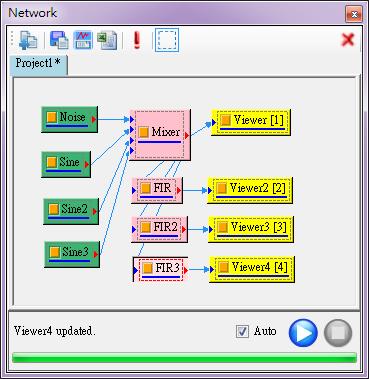
10 The picture above shows the symbol-editing menu that comes up after right-clicking the module compiling area. The menu is divided into five major groups, Compute, Conversion, Source, Viewer, and Writer. The component of each module describes its method of operation and Chapters 2, 3, and 4 go into each method in more specific detail. The components editing area works like a flow chart controlling operations of the signal processes you want analyzed. By connecting the signals and modules in the way you choose, complex signal analysis is possible in a few simple steps. With these options, Visual Signal will give you the ability to analyze signal processes, signal front-end processes, signal analysis algorithms and render them into visual graphics. Below is an example of what a typical signal analysis project could look like. 8

11 If there is a problem with the connected components, the Network Window will display a flashing warning sign ( ) or an error sign ( ) over the component. Placing the mouse over the sign will display a tooltip describing the detail of the problem. Double-clicking the error sign will place the warning inside the project which is helpful if you have multiple errors to keep track of at once Component Editor Toolbar The component editor toolbar is responsible for data operation commands such as inputting and outputting data and are listed below: Import data from file Save data to file Open Data Viewer Export data to Excel Descriptions of each command are listed below: 9

12 1. Import data from file: This command makes Visual Signal read import data from an external file. Acceptable file formats are Time Frequency Analysis file, plain text (ASCII file), and a variety of other different formats. If the file is in plain-text format or comma separated values format, the Text Importer window will appear for you to set up information for the data. File Extension tfa txt uff vsb eeg csv wav, mp3, aac, ac3, mp4, m4a, amr, ape, wma dat File Type Time Frequency Analysis File Plain text file Universal file format Binary file for Visual Signal SleepScan and Ceegraph EEG data file Comma-separated values Audio files ADLINK DAT file If you want to import a data file that is not in a supported format a warning message will appear asking you if you want to read the file in plain text format. Selecting yes will bring up the Text Importer to attempt to read the file. You must use the Text Importer to setup the signal timeline, such as units of time, the sampling range, and the data range. A more detailed explanation of this feature is in Section Save data to file and Export data to Excel These two commands save the data in the file format tfa, txt, and csv etc. Sound signals can be saved as a wav file or other audio formats. These two features are mainly used in the Writer function and are explained in more detail in Section 4.5 Writer (Signal Output Modules). 3. Open Data Viewer This command opens the data viewer window which allows you to select the components of calculation results. Also allows you to view the data browser which will detect the output data type, automatically adjust the way the data is presented, 10

13 and display graphics with data of the output device. This command is described further in Section Force update Click to execute the project from start to finish including all module components Operation Control Area The Operation Control Area is located below the Components Module Compiling Area and controls and displays the calculation process. The text on the left side is the calculation process in real-time, displaying the percentage of progress made in the implementation of the current program while the text below the progress bar immediately displays the progress of the current component being calculated. There are three controls on the right to provide you with control over the computing process, and are described below: 1. Auto function This function determines whether or not the program will be updating the calculations in real time as you modify them. If the Auto box is checked, whenever the user changes device parameters the program will immediately recalculate the components and all of the following components in the component output port. You may encounter a situation where you need to modify multiple components before wanting the program to update after each change, if that is the case uncheck the Auto box. 2. Perform operation If the Auto button is not checked, then pressing the perform operation button will have the program run the modified components. Compared to the Auto option this can be looked at as a Manual option. 11

14 3. Abort operation If program is in the course of running operations and you want to terminate the processes you can press the abort operation button. Something to note though is that this feature only terminates the components of a single process and thus only one element and its following processes will be terminated, the program will still continue the implementation of the other components Data Viewer There is lots of information that needs to be shown such as component outputs, data types, query signals, etc., so we provide a fast tool to view that data with the data viewer. The interface of the data viewer window shows the data value, waveform, and signal information as long as their components are in the component editor. Click a specific component and press the data viewer button and the browser will accommodate the different signal types (such as signal spectrum analysis results, numeric data or timefrequency analysis) and display relevant information. The browser window interface will correspond to the different signal types being used Visualization Window The Visualization Window is where the diagrams appear after creating a viewer component in the Network Window. In this window you will have a few options available to customize your diagrams and we will go through them in this section. More detailed customization is done through the Property Window and is covered in Section 1.5. Note: The group/move options located in the top left will only show up when your curser is hovering in that area. Above is an example of audio signal displayed by a basic Channel Viewer diagram. The red outline around the diagram signifies that the diagram is currently being selected in the Network Window. Because this is an audio file, there are five options located in the top right that allow you to continuously Loop (if box is checked), Mute, Play, Pause, or Stop the audio file and will only show up if the data is in audio format. 12

15 When a diagram is selected (as indicated by the red outline around it) scrolling the mouse wheel will zoom in and zoom out the x-axis for more specific viewing. To select a specific diagram, you can either click the diagram directly or click the viewer component it is associated with in the Network Window. Double-clicking the viewer component will bring up Plot Element Setting window which allows you to choose whether or not a certain channel is displayed, the channel name, and what type of color and line will be associated with the channel. This is very useful when working with a diagram that has multiple channels. Note: Clicking Display All or Hide All will either check all the boxes under Display or uncheck them all. Hovering your cursor in the top left of a diagram gives you the options to Delete, Move, or Group your diagram. Checking the Group box gives you the option of placing the specific diagram in a group numbered 1-5 and choosing whether to sync the X axis, the Y axis, or both with other diagrams in the same group. Right-clicking a diagram will bring up a list of options dealing with going back to specific views of the diagram and how to export the specific diagram into other areas. The first three options View Home, View Prev, and View Next deal with viewing the diagram after making edits such as zooming in and out. View Home brings the diagram back to its default view, View Prev can be compared to an undo button while View Next is a re-do button. 13

16 The next set of options deal with exporting the specific diagram to other programs or documents. The first two options, Copy to Clipboard (Bitmap) and Copy to Clipboard (Metafile) place the diagram on your clipboard to easily paste it into a program or document. Export to file allows you to save the diagram as a file in multiple picture formats. Print will bring up a print settings window for you to directly print the diagram Property Window The Property Window shows the properties of whichever diagram you are selecting in the Visualization Window or whichever component in the Network Window. When you select something the Property Window will display a list of its properties that can be edited either through manual typing or through a drop down menu. You can also see what module the program is using for its computations. Note: When the arrow to the left of a section is black the options are being shown, when it is clear the options are being hidden. Clicking the arrow will either expand the list or contract it. The bottom of the Property Window gives a detailed explanation of what editing each property will affect and is very helpful if you don t know what a certain property does Properties of a Diagram Selecting a diagram from the Visualization Window will bring up its properties in the Property Window. Details of the diagram can then be altered to suit your needs. Almost every aspect of your diagram can be changed from the Property Window. It is important to note that if you do not know what changing a certain property will do, the bottom box in the Property Window gives a detailed explanation of what the property does. Appearance The first section of properties dealing with your diagram has to do with its appearance. Here you can specify the background color and the height or width of your diagram. 14

17 The ListOrder specifies where the diagram is listed in your Visualization Window and RetainPlot. Channel This section allows you to choose how many input channels are in your diagram but also depends on how many input channels your specific type of diagram can support. Fonts and Colors Here you will be able to change the fonts and colors of all the text in your diagram from the title to the axes. Grid This section allows you to make changes to the grid overlay behind the data. Many of the spacing/anchor is already set to Auto by default which makes the program calculate the best fit for the diagram. If you change the value and want to restore it to its default, type Auto again. Module This property menu shows the details of the module being used. You will be able to see what class of viewer is being used, the time it took to execute, and the acceptable data types it can use. You can also change the name of the module to make organizing your Network Window easier. 15

18 Representation This section allows you to edit how your data is represented in the diagram. You will have options such as adding a legend, specifying what type of axes to use and what maximum and minimum values to use for your axes. Title Here is where you will be able to change the labels on your title, x-axis, and y-axis. Typing in {default} will revert back to the original label and typing {all} will show the whole title. You may also use the index to show which component name you want to see Properties of a Component Selecting a component from the Network Window will bring up its properties in the Property Window. Every component in the Network Window has options that can be modified from the properties. The Property Window also displays detailed information about the component. For example if you select a data component, the Property Window will list where the file location is, how many channels are in the data, the sampling frequency, etc. Depending on which component you have selected, different options will be available to modify. There is never one set way to analyze data and is why these options are made available to you. In this section we will use examples from a compute component and a convert component. The first example shows the properties of a Conversion Convert to Regular component. Here you will have options relating to how you want to convert your indexed into regular data. For example, convert method allow you to 16

19 choose whether you want the sampled data to be filled in by missing points or for the gaps to be removed. If you don t know what a certain property does remember that when it is selected a brief description will appear in the bottom box of the Property Window. The second example shows the properties of selecting a Compute TFA ShortTerm Fourier Transform component. You will see a different set of properties than the Convert to Regular component as different components have different sets of modifiable properties. In this set of properties you can customize how you want the specific ShortTerm Fourier Transform component to operate. Maybe for your first transformation you want a linear axis as the frequency type and a log axis for your next transformation, all these details are modified from the Property Window The Module section of these components is similar to the diagram module section. Specific information will be shown about the module being used for the component such as the class module, the execution time, the acceptable data types, and its output 17

20 data types. You will also have the option to change the name of the module and its input and output port side. 18

21 1.2 Importing Your Data 1. Importing data is done by going to the Network Window and clicking Import data from file. 2. Locate your data file and see if it is a supported format, if it is not the program will ask you if you want to use Text Importer to format the data. 3. Once the Text Importer window is opened, a preview of how your data will be formatted will be under File Contents near the bottom of the window. This preview will adjust in real-time as you make changes to the options. 4. Start by specifying the data range of your data. Here is where you specify which rows and columns you want your data to start and end at and whether you want the direction of the data to be column-based or row-based. By default the data will be separated into multiple channels depending on how your data is formatted, but by clicking the Concatenate to one channel checkbox your data will be set as a single channel regardless of how many columns or rows you have. You can 19

22 also specify which axis is your time axis by checking the Specify Time Axis box and choosing the corresponding axis. 5. Next area is the Field Format which will determine how the data will be separated. The default option is Any whitespace which will separate the data each time there is white space between them. The Delimiter option allows you to choose specific symbols that separate the data. If you want to specifically format the data yourself, you can use the Fixed Field option and see how it will be formatted in the file contents section. The import data can be merged to complex by checking Complex check box. 6. In the event that there are null-values in your data set, there is a Handle Null- Values option that is checked by default. Here you can choose how Visual Signal will handle your null-values when it imports your data set as there are a variety of options such as having fixed values or having Visual Signal calculate a linear interpolation. 7. The next set of options has to deal with the Time Coordinate. Specify the unit of time your data set uses by selecting the options under Time Unit. If you need to shift will also be able to choose the Sampling Frequency and whether or not you need to down sample your data set in the case your amount of data is too large and you want to reduce the number of sampling points to make computation easier. 8. The final sets of options are related to adding dates to your data set. The default option checked is Auto which will check if you have dates associated with your data and will set up accordingly. If you want to add dates manually check the Enable box and specify the starting date and time options to its right. After you are finished adjusting all the settings press import and your data should show up as a component in the network window. 20

23 Chapter 2 Example Projects 2.1 Your First Project This section will go through an example of how you would start a project, use the modules, and export your new diagrams. In this example we will take raw frequency data from the audio file WindowsXP.wav, which is located in C:\Program Files\AnCAD\Visual Signal\demo\Basic, compute a ShortTerm Fourier Transformations and display two separate time-frequency spectrograms usable in a document or presentation. 1. Select File New Project from the toolbar. 2. Go to the Network Window and click Import data from file 3. Navigate to C:\Program Files\AnCAD\Visual Signal\demo\basic and open the file WindowsXP.wav. Note: File locations will be different depending on platform (x86 or x64) or the installation path you selected. 21

24 4. Check the Specify Time Axis box and click Import, the settings should like the picture below. 5. A warning will pop up saying the data is Indexed and should be converted to Regular. Click Okay. 6. A green component named Windows XP will now be in the Network Window, right-click the box and select Viewer Channel Viewer. Note: Hovering your curser over an option or component will show details on what the option does. 22

25 7. A Channel Viewer component will now be linked to the Windows XP component by an arrow and a graph will be displayed in the Visualization Window. The graph shows that the data set has two separate channels and is shown by the two different colors. Note: Clicking on the square inside a component disables/enables the component, while clicking the component directly as shown in the picture above outlines in red the specific graph the component is associated to. 8. Right-click the Windows XP component and select Compute Channel Channel Switch. Repeat this step so you have two switch components linked to the Windows XP component. 23

26 9. Click on the Switch2 component. Locate the Active Channel section under the Property Window. Click the arrow on the right of 1:CH1 and click 2:CH2 from the drop down menu. 10. Right-click the newly made Switch component and select Viewer Channel Viewer. A new diagram will appear in the Visualization Window with the option to listen to the audio. Do the same thing to the Switch2 component. 11. Right-click the Switch component and select Compute TFA ShortTerm Fourier Transform. 12. Right-click the STFT component and select Viewer Time-Frequency Viewer. A time-frequency spectrogram will now show up under the Visualization Window. 13. Repeat steps 11 and 12 for the Switch2 component. You will now have two time-frequency spectrograms in your Visualization Window. Following these steps should yield a Network Window similar to the figure below. 24

27 14. Select the TF Viewer [4] component. The Visualization Window should now bring up the first time-frequency spectrogram. Right-click the diagram and select Copy to Clipboard (Bitmap). The diagram will now be copied onto your clipboard and can be pasted in documents or presentations. 25

28 2.2 Spectrum Analysis Setting Up and Analyzing a Fourier Transformation In this section we will go through an example of how to set up a Fourier analysis of a sine function. 1. Right-click the component editor window inside the Network Window and select Source Sine Wave. 2. Right-click the new component labeled Sine inside the Network Window and select Viewer Channel Viewer. This will display a graph of a sine wave that you can analyze and modify in the Property Window. In this example we will keep the sine wave as default. 3. Right-click the component labeled Sine again and select Compute Transform Fourier Transform. 26

29 4. Right-click the new FFT component and select Viewer Channel Viewer. A graph of the Fourier transformed sine wave will now be displayed in the Visualization Window. 5. On the graph that you just created labeled Sine-FFT click inside the graph and drag your mouse cursor from the second notch in the x-axis and to zero as if you were highlighting the triangle in the graph. This will zoom in the graph to the section you highlighted. 6. Double-click the Viewer [1] component and select the circle from the Marker Style drop down menu in the Plot Element Setting window, then hit Ok. 7. The graph will now be marked with circles at every frequency point. You should notice that the main curve is only made up of three points, creating a jagged curve. To achieve a more accurate curve we need to add more frequency points that make up the curve. 8. Select the FFT component and locate the Resolution setting in the Property Window. This is the multiplication factor of frequency resolution of the Fourier transform. Increasing the number will increase the number of frequency points resulting in a smoother curve. Replace 1 with 35 and highlight the curve on the graph like you did in step 5. Before After 27

30 9. The curve now has side lobes as a result of the multiplication factor but we can fix this by selecting a window function to apply before the Fourier transformation. Select the FFT component and locate the Window setting in the Property Window. Then select the Hanning option from the drop down menu. 10. Double-click the Viewer [1] component and select None under the Marker Style to remove the circle indicators. 11. Click the Show Value button in the toolbar then place your mouse cursor over any section of the curve. This will allow you to analyze the values of the curve with your mouse cursor. The values are displayed on the bottom-left corner of the Visualization Window. 12. Click the button to the right of the Show Value button with the drop down menu to select Pick Maxima. The value cursor will now lock to the nearest maxima on the curve making it easier to find specific values. 28

31 13. To leave the Show Value mode, select the Rect Zoom buttons in the toolbar. 14. Click and drag a rectangle over the curve, the graph will then zoom in to the area inside the rectangle. 15. Using the other zoom functions in the toolbar will make it easier for you to display specific areas of the curve. 29

32 Chapter 3 Data Acquisition Quick Start Data acquisition is the process of sampling signals that measure real world physical conditions and converting the resulting samples into digital numeric values that can be analyzed on the computer with programs such as Visual Signal. Visual Signal works in conjunction with a variety of data acquisition systems (DAQ) such as ADLINK that allows real-time data acquisition and the ability to convert the recorded analog waveforms into digital values for processing. The data can be directly sampled from within Visual Signal for simple accessibility and manipulation. This user guide will go through examples of how to integrate the ADLINK data acquisition system with Visual Signal and how to record audio with your computer. 3.1 Recording Audio with Computer This section will go through an example of how to record and analyze an audio signal recorded from your computer microphone. If your computer has a microphone, you can directly record an audio signal into Visual Signal to analyze. 1. Right-click the Network Window and select Source DAQ Audio-DAQ. 30

33 2. Double-click the Audio-DAQ module to open the Audio Card DAQ window. Under the Audio Card tab select the input device for your microphone from the drop down menu under the Input Device option. You can adjust the volume of your microphone by clicking on the System Dialog button next to Mic Volume. This will open up your microphone properties and allow you to make proper adjustments. Next select the bit rate of your recording under Bits Per Sample and then choose whether you want a Stereo or Mono channel. You can then test your microphone by looking at the microphone level bars for the left channel (capital letter L ) and right channel (capital letter R ). 3. Once your microphone is set up and the settings of your recording are correct click the Data Acquisition tab. Here you will have two options for recording your audio. The first option is recording for a set amount of time that you set under the Sample Time(s) in seconds. The second option is checking the Continuous Mode option, this option constantly records audio and displays the data in real-time until stopped by clicking the square button (Stop button) in the network window. The Sample Rate (Hz) applies to both options of recording. 31

34 3.1.1 Recording audio data in a set amount of time (Option 1) 1. Set the amount of time you wish to record for in the Sample Time (s) section in seconds. 2. Select the sound quality of your recording by adjusting the Sample Rate (Hz). The higher the sampling rate, the higher the sound quality. The standard sampling rate of most recordings is Hz. 3. The Data Length is the number of points recorded during the recording. Typically, this does not need to be changed as it will automatically update on its own based on your sample time and sample rate. 4. Click the red circle (Record button) when you are ready to begin your recording. 5. After the recording is finished, the data will be stored inside the Audio-DAQ component. From here you can attach a Channel Viewer by rightclicking the component and selecting Viewer Channel Viewer to view the recording and play the recording back. 6. Right-click the Audio-DAQ component and select Compute Transform Fourier Transform. This will convert the audio 32

35 recording into the frequency domain. Right-click the FFT component and select Viewer Channel Viewer to view the resulting graph Recording audio data in real-time (Option 2) 1. Right-click the Network Window and select Source DAQ Audio-DAQ. Attach a Channel Viewer to the Audio-DAQ component if you want to view the recording in a time vs. amplitude graph or attach a time-frequency viewer if you want to view the recording in a time vs. frequency graph. 2. Double-click the Audio-DAQ component and select the Data Acquisition tab. 3. Check the Continuous Mode box under DAQ. 4. Select the sound quality of your recording by adjusting the Sample Rate (Hz). The higher the sampling rate, the higher the sound quality. The standard sampling rate of most recordings is Hz. When DAQ mode is checked the sample time and data length option will be disabled and grayed out since it will automatically be calculated for you. 5. Change the refresh rate of the graph and the data length by adjusting the Cont. Update Rate (Hz). The higher the update rate, the lower the 33

36 data length. If you want to get a finer resolution in the spectrum or spectra, the data length should be longer. So setting a higher update rate will result in a higher refresh rate in the graph. Set a lower update rate to get a finer resolution. 6. Select the type of scrolling mode you want when the data is represented on your attached viewer. The way scrolling works is that for every n data points sampled, which is decided by setting Cont. Update Rate (Hz), only one data point is used for plotting, and the scrolling mode allows you to choose how you pick that one data point. The different modes include Off, Sample, Average, Extrema, and STFT. Off : This mode will have no scrolling and will represent whatever audio signal is currently being recorded on the viewer. Sample : This mode picks the first point of the data sampled and plots the point. Average : This mode takes the average of the n points and plots the point. Extrema : This mode picks the point with the largest absolute magnitude of the n points and plots the point. STFT : This mode will output time-frequency data in real time and requires you to attach a time-frequency viewer instead of the standard channel viewer. 7. Once your settings are set, you can decide whether or not you want to have the recording saved to a specific file by checking the Logging box and specify the name and location. If the specified file already exists, the old content will be replaced by the new file. 8. Click the red circle (Record button) when you are ready to begin your recording. 9. Visual Signal will now go into Real-Time Mode Updating which means data is constantly being recorded into your Audio-DAQ component. The viewer 34

37 you attached to the module will constantly be updated to show you the recorded data in real-time. To finish recording, press the stop button in the network window. 10. After the recording is finished, the data will be stored inside the Audio-DAQ component. Right-click the Audio-DAQ component and select Compute Transform Fourier Transform. This will perform a Fourier transform and convert the audio recording into the frequency domain. Rightclick the FFT module and select Viewer Channel Viewer to view the resulting graph. 35

38 3.2 Using ADLINK In order to use the ADLINK hardware with Visual Signal, the latest driver for the device must first be installed. UD-DASK is the kernel driver for the ADLINK hardware and has support for 32-bit/64-bit Windows 7/Vista/XP OS. Please note that only UD-DASK versions and later can support the USB-2405 module Installing the UD-DASK Driver 1. Locate the file named UD-DASK. This will be in the driver installation CD provided with the device or you can download the latest driver from The latest version at the time this guide was created is v Note: a. Make sure you are the Administrator of the computer or have administrative privileges. b. Confirm you have the latest driver installed to ensure your device works properly. 2. Once the installation wizard is opened, click Next. 36

39 3. Click Next to install to the default folder, or click Change to install to a different location. 4. Press the Install button to begin the driver installation process. 5. During the installation process, Windows will verify the installation the driver. Check the Always trust software from ADLINK TECHNLOGY INC. and click Install. 37

40 6. Once the installation process is done, click Finish to close the wizard. 7. A prompt will ask to restart your computer to finalize the installation, click Yes Connecting the device 1. Connect the ADLINK USB DAQ module to a USB port on the computer using the included USB cable. 2. The first time the device is connected, a New Hardware message will appear. It will take around one minute to load the firmware. When loading is complete, the LED indicator on the rear of the USB DAQ module changes from amber to green and the New Hardware message will close. Note: There are two requirements to starting Visual Signal DAQ Express. a. The driver must be installed properly. b. The hardware (ADLINK USB-DAQ 2405) is connected. Note: If any of the following requirements are not met, the following error message will appear. 38

41 3. The USB DAQ module can now be located in the hardware Device Manager. Note: If the device cannot be detected, the power provided by the USB port may be insufficient. The device is exclusively powered by the USB port and requires V Recording data with device 1. Open Visual Signal DAQ Express. 2. Right-click the Network Window and select Source DAQ Adlink-DAQ. Attach a Channel Viewer to the Adlink-DAQ component if you want to view the recording in a time vs. amplitude graph or attach a TF Viewer if you want to view the recording in a time vs. frequency graph. 3. Double-click the Adlink-DAQ component to open the Adlink DAQ Window. 4. In the Adlink DAQ Window, select which channels to record from. 39

42 Note: If you have your sensor connected to channel 0 on the device, it will be channel 1 in Visual Signal. ADLINK devices start at channel 0, while Visual Signal starts at channel Adjust any settings such as the Coupling, Input Type, IEPE, and Scale to work with the signal you are analyzing. Note: Refer to the ADLINK User Guide for detailed explanations of these functions. 4. Once you are finished with selecting the channels to use and the settings click the Data Acquisition tab. Here you will have two options for recording your signal. The first option is recording for a set amount of time that you set under the Sample Time (s) in seconds. The second option is checking the Continuous Mode option, this option constantly records signals and displays the data in real-time until stopped by clicking the square button (Stop button) in the Network Window. The Sample Rate (Hz) applies to both options of recording. 40

43 Recording signal data in a set amount of time (Option 1) 1. Set the amount of time you wish to record for in the Sample Time (s) section in seconds. 2. Select the sample rate of your recording by adjusting the Sample Rate (Hz). The higher the sampling rate, the more sample points a second resulting in more accurate signals. The highest sampling rate of the ADLINK device is Hz. 3. The Data Length is the number of points recorded during the recording. Typically, this does not need to be changed as it will automatically update on its own based on your sample time and sample rate. 4. Click the red circle (Record button) when you are ready to begin your recording. 5. After the recording is finished, the data will be stored inside the Adlink- DAQ component. From here you can attach a Channel Viewer by rightclicking the component and selecting Viewer Channel Viewer to view the signal. 41

44 6. Right-click the Adlink-DAQ component and select Compute Transform Fourier Transform. This will convert the signal into the frequency domain. Right-click the FFT module and select Viewer Channel Viewer to view the resulting graph Recording signal data in real-time (Option 2) 1. Right-click the Network Window and select Source DAQ Adlink-DAQ. Attach a Channel Viewer to the Adlink-DAQ module if you want to view the signal in a time vs. amplitude graph or attach a TF Viewer if you want to view the recording in a time vs. frequency graph. 2. Double-click the Adlink-DAQ component and select the Data Acquisition tab. 3. Check the Continuous Mode box under DAQ. 42

45 4. Select the recording quality by adjusting the Sample Rate (Hz). The higher the sampling rate, the more accurate the resulting signal will be. The highest sampling rate of the device is Hz. When DAQ mode is checked the sample time and data length option will be disabled since it will automatically be calculated for you. 5. Select the desired Cont. Update Rate (Hz) 6. Select the type of scrolling mode you want when the data is represented on your attached viewer. The way scrolling works is that for every data points sampled, only 1 data point is used for plotting, and the scrolling mode allows you to choose how you pick that one data point. The different modes include Off, Sample, Average, Extrema, and STFT. Off : This mode will have no scrolling and will represent whatever audio signal is currently being recorded on the viewer. Sample : This mode picks the first point of the data sampled and plots the point. Average : This mode takes the average of the 1024 points and plots the point. Extrema : This mode picks the point with the largest absolute magnitude of the 1024 points and plots the point. STFT: This mode will output time-frequency data in real time and requires you to attach a time-frequency viewer instead of the standard channel viewer. 7. Once your settings are set, you can decide whether or not you want to have the recording saved to a specific file by checking the Logging box and specify the name and location. If the specified file already exists, the old content will be replaced with the new file. 43

46 8. Click the red circle (Record button) when you are ready to begin your recording. 9. Visual Signal will now go into Real-Time Mode Updating which means data is constantly being recorded into your Adlink-DAQ component. The viewer you attached to the component will constantly be updated to show you the recorded data in real-time. To finish recording, press the stop button in the Network Window. 10. After the recording is finished, the data will be stored inside the Adlink-DAQ module. Right-click the Adlink-DAQ component and select Compute Transform Fourier Transform. This will perform a Fourier transform and convert the recording into the frequency domain. Right-click the FFT component and select Viewer Channel Viewer to view the resulting graph. 44

47 45

48 Chapter 4 Function List 4.1 Computing With Signal Flow Object Channel 1. Channel Switch: Select a single-channel from a multi-channel source. 2. Data Selection: Select a time frame from a source data to be analyzed. 3. Fill NULL Value: Use mathematical methods to fill any data that is missing (known as NULL value). 4. Input Switch: Accept all sorts of input signals, and one signal is chosen. 5. Remove Channel: Remove a single-channel from a multi-channel source. 6. Replace Value: Replace a particular value in the signal data. 7. Resample: Set a new sampling frequency value to a signal data. 8. Time Shift: Shift the graph along the x-axis (time). 46

49 Channel Switch Select a single-channel from a multi-channel source. Properties This module accepts input of Signal (which could be a real number or complex number, multiple-channel, Regular or Indexed), numeric (which could be a real number or complex number, multiple-channel, Regular or Indexed), and Audio (which could be real number or complex number, multiple-channel, Regular). The output formats are real numbers or complex numbers, single channel, and Regular signals. The properties and settings of the Channel Switch are introduced below. {Channel Switch} Property Name Channel Count Property Definition Shows the number of channels currently connected to components Default Value Positive integer Active Channel Select the active channel Channel 1 (the 1 st channel) If Select Last Channel is set as True, Select Last Channel then the channel to be removed will always be the False last channel Example Combine a sine wave data with a triangle wave data into multi-channel and use Channel Switch to select one of the signal waves to display. 1. Create a Source Sine Wave and a Source Triangle Wave and connect the two components into a Conversion Merge to Multi- Channel to create a multi-channel signal data. 47

50 1 (Sine, Triangle) - ToMulti Time [sec] Change the SamplingFreq of both Sine and Triangle component to 1000, SignalFreq to 6 and 15 respectively. 2. Output ToMulti component to a Channel Viewer component. In the Channel Switch component, you can change the Active Channel to 48

51 1:Sine_CH1 or 2:Triangle_CH1 to read either the sine wave signal or the triangle wave signal. 1 (Sine, Triangle) - ToMulti - Switch Time [sec] 49

52 1 (Sine, Triangle) - ToMulti - Switch Time [sec] Related Functions Merge to Multi-Channel, Channel Viewer, Source 50

53 Data Selection Select a time range from a source data to be analyzed. Properties This module accepts input of Signal (which could be a real number or complex number, single channel or multi-channel, Regular) and Audio (which could be a real number or complex number, single channel or multi-channel, Regular). Enter the selected range of the signal by defining the StartPosition and EndPosition (time unit). You can also move your cursor near the entering field and the button will show up. Click the button at the right side of the field to enter the Data Viewer and select the range by mouse. {Data} Property Name SamplingFrequency DataCount {Data Selection} Property Name StartPosition EndPosition Property Definition Displays the sampling frequency of the input data Displays the sampling count of the input data Property Definition Enters the value of the start position of the input data Enter the value of the end of the input data Default Value 0 0 Default Value The original start time for the input data The original end time for the input data 51

54 DownSampleStep Example NewCount Reduce the sampling frequency of a signal by dividing an integer Display the new data count re-calculated by selected interval and DownSampleStep Create Source Sine Wave and connect it to Viewer Channel Viewer. 1 Sine Time [sec] In this Sine component the SamplingFreq is 1000 and the SignalFreq is Connect a Compute Channel Data Selection to the Sine component then connect it to Viewer Channel Viewer. In Selection component set the StartPosition to and EndPosition to and the new graph will be show the range between to (The original range is between, so the new range has to be within the original range.) 52

55 1 Sine - Selection Time [sec] 3. The range will now be between and the NewDataCount is 201. Try using DownSampleStep to reduce sampling frequency. By setting DownSampleStep to 5, the sampling frequency of the sine wave will change to 200 from 1000 and the NewDataCount will be 41. This will cause the curve of the sine wave to become rough. 53

56 1 Sine - Selection Time [sec] How to select a data range with Data Viewer 1. Click to enter the Data Viewer. The top graph is the full signal where the range can be selected by dragging your mouse over the desired area. After selecting your range, the selected data will be shown within two red vertical lines as indicated in figure below. The second graph shows the partial data which you selected. 54

57 2. After deciding the range, click to extract the data. The Selection component will automatically import the selected value of StartPosition and EndPosition. Related Functions Data Viewer, Channel Switch, Channel Viewer, Source 55

58 Fill Null Value Use a mathematical method to fill any data that is missing with the NULL value. Introduction To fill in the data signal or NULL values., which contains NaN (Not a Number) Properties This module accepts input of Signal (which could be a real number, single channel or multi-channel, Regular or Indexed) and Audio (which could be a real number, single channel or multi-channel, Regular). In the FillMethod, there are six methods to fill in the missing values. {Fill Null Value} Property Name FillMethod NullValue Property Definition There are the FixedValue, PrevValue, NextValue, LinearInterpolation, SplineInterpolation, and MonotonicCubic methods to fill the NULL value Enter a value to replace all the NULL values. Default Value LinearInterpolation 0 56

59 Variable Option FixedValue PrevValue NextValue LinearInterpolation SplineInterpolation MonotonicCubic Property Definition A new NullValue variable option will appear in the Properties Window. Enter a value to replace all the NULL values to the values entered The NULL value will be replaced with the previous value in the signal The NULL value will be replaced with the next available value in the signal Using linear interpolation to calculate the value of the NULL Using spline interpolation to calculate the value of the NULL Monotone cubic interpolation is a type of cubic interpolation that preserves monotonicity of the data set being interpolated. MonoticCubic method is better than SplineInterpolation method when the slope of the signal is large e.g. Square Wave Example To fill in the missing values using Fill NULL Value component. 1. Open demo53 in the directory C:\Program Files\AnCAD\Visual Signal\demo. From the graph in the Visualization Window, you can clearly see the missing values on the graph. Note: File locations will be different depending on platform (x86 or x64) or the installation path you selected. 2. Connect the source signal data to Compute Channel Fill NULL Value and select LinearInterpolation in the FillMethod of the Fill NULL Value component. 57

60 2 test3_nan - FillNull - Linear Time [sec] 3. Select SplineInterpolation method instead and the way the values are filled in will be considerably different. 2 test3_nan - FillNull - Spline Time [sec] 4. In the Text Importer there is also an option to fill in the missing value but this feature is different from the Fill NULL Value component. 58

61 5. Import a data which has missing values and intentionally uncheck the box Handle Null-Values in Text Importer. The imported value and graph is shown in the image below. 59

62 1 Square Time [sec] 6. Now create two Fill NULL Value components to connect to the imported source signal data, where Square Wave has some removed points. The first component will use the SplineInterpolation fill in method and the second component will use the MonotonicCubic fill in method. 7. From the results shown in the Channel Viewer, there is an obvious difference between the SplineInterpolation method (thin dark line) and the MonotonicCubic method (thick blue line). 1 (Square - FillNull, Square - FillNull2) Time [sec] Related Functions Text Importer, Resample, Channel Viewer, Source 60

63 Input Switch Select one channel from a multi-channel input signal. Properties This module accepts input of Signal (which could be a real number or complex number, single channel or multi-channel, Regular or Indexed), Audio, numeric, and spectra. The definition and default value of the parameters are shown below. {Input Switch} Property Name Input Count Active Input Property Definition Total number of channels in this component Default Value The selected channel number 1 0 Example Use Source Noise as the source signal, carry out different calculations on it and output the results in a different format. Then use Input Switch to select one of the channels. 1. Create Source Noise in Network Window. In the Property Window set TimeLength to 3, set SamplingFreq to 1000, and set Amplitude to Connect the Noise component to Compute TFA ShortTerm Fourier Transform, Compute Transform Fourier Transform, and Conversion Convert to Audio, respectively. 61

64 3. Connect all outputs of the calculations to Compute Channel Input Switch, and view the result with a Channel Viewer. Change the Active Input setting in Input Switch to view different results. 62

65 Frequency [Hz] V I S U A L S I G N A L E X P R E S S G U I D E 4. Connect Input Switch to Viewer TFA Viewer and change the Active Input setting to observe the result of the STFT. 500 Noise - STFT Time [sec] Related Functions Fourier Transform, Convert to Audio, ShortTerm Fourier Transform, Time-Frequency Viewer, Source 63

66 Remove Channel Remove a single-channel from a multi-channel source. Properties This module accepts input of Signal (which could be a real number or complex number, multi-channel, Regular or Indexed) and Audio (which could be a real number or complex number, multi-channel, or Regular). {Remove Channel} Property Name Channel Count Remove Channel Select Last Channel Property Definition Default Value Displays the number of channels 0 Select the channel to be removed Channel 1 If Select Last Channel is set as True, then the channel to be removed will always be the last channel False Example Combine a sine wave, a triangle wave and a square wave together, connect it to a Remove Channel component and remove the sine wave. 1. Create Source Sine Wave, Square Wave and Triangle Wave and connect them all to a Conversion Merge to Multi-Channel to make the three waves into a multi-channel signal data. Set the SamplingFreq as 1000 and set the Sine component s SignalFreq as 5, Square component s SignalFreq as 8 and Triangle component s SignalFreq as 15 and observe the different waves on the graph. 64

67 1 (Sine, Square, Triangle) - ToMulti Time [sec] 2. Connect the Merge to Multi-Channel component to Compute Channel Remove Channel and set Remove Channel as 1:Sine_CH1 (sine wave). 65

68 1 (Sine, Square, Triangle) - ToMulti - RemoveCh [Ch1] Time [sec] 3. Now set the Select Last Channel as True and you will see that Remove Channel will automatically change to 3:Triangle_CH3 and the triangle wave signal (Channel 3) will be removed. 66

69 1 (Sine, Square, Triangle) - ToMulti - RemoveCh [Ch3] Time [sec] Important Note Channel Switch and Remove Channel are completely opposite functions. Channel Switch preserves a single selected channel from a multi-channel signal data and Remove Channel removes the single selected channel from a multichannel signal data. Related Functions Merge to Multi-Channel, Channel Switch, Source 67

70 Replace Value Replace a particular value in the signal data. Properties This module accepts input of a signal (which could be a real number, single channel or multi-channel, Regular) and Audio (which could be a real number, single channel or multi-channel, Regular) and replaces specific values to another value. {Replace Value} Property Name ReplaceMethod Condition Expression Replace Value Type ReplaceValue StartPosition EndPositon Outlier Boundary Property Definition There are All, Expression, Outlier, and ByPass methods to replace value. Use the conditional expression to replace value. The arithmetic operators are available to use. Only for Expression mode. There are three kinds of value types, Custom, NULL, mean, and median. Set the value which signal data will be replaced with. The start position of x-axis to begin replacing. The end position of x-axis to end replacing. The multiples of the standard deviation. Only for Outlier Default Value Expression y = null Custom 0 The start point of the input signal. The end point of the input signal. 3 68

71 Sliding Window Mode Example mode. True sets the sliding window which is used for the Outlier mode. Only for Outlier mode. False Change the maximum value of the square wave to another number 1. Create a Source Square Wave and connect it to a Viewer Channel Viewer. 1 Square Time [sec] 2. Now connect the Square component to Compute Channel Replace Value and modify the Condition Expression to y==1. Then set the ReplaceValue to -0.5, StartPosition to 0.2, and EndPosition to 0.6. Now all the values in of the square wave which were originally 1 will become

72 -1 Square - Replace Time [sec] 3. Change Replace Value Type to Null, Mean, or Median and observe the difference between these types. Null, Mean, and Median will replace values with a null value or the mean or median of a specified range, refer to the bottom figures to observe the differences. 70

73 1 Square - Replace(Null) Time [sec] 1 Square - Replace(Mean) Time [sec] 1 Square - Replace(Median) Time [sec] Important Note You can only replace one value at a time. If you want to replace multiple values then several Replace Value components will have to be created. Related Functions Source, Channel Viewer 71

74 Resample Resample allows you to set a new sampling frequency value to a signal data. Properties This module accepts input of Signal (which could be a real number or complex number, single channel or multi-channel, Regular) and Audio (which could be a real number or complex number, single channel or multi-channel, Regular) {Data} Property Name Property Definition Default Value FrequencyUnit Sampling frequency unit of input data None SamplingFrequency Sampling frequency of input data 0 DataCount Sampling count of input data 0 {Resample} Property Name Step Downsampling ReSamplingMethod Property Definition If set to True, the input data will be down-sampled with DownSamplingStep Select a resampling interpolation method: Nearest, Linear, Spline, and MontonicCubic Default Value True 72

75 DownSamplingMethod DownSamplingStep NewSamplingFrequency NewCount Select a down-sampling method: Sample, Average, MaxDetect, MinDetect, or PeakDetect Set the integer ratio for downsampling if Step Downsamping sets True Set the new sampling frequency Display the new sampling count of the data output Sample {DownSamplingStep} Variable Option Sample Average MaxDetect MinDetect PeakDetect {ReSamplingMethod} Variable Option Nearest Linear Spline MonotonicCubic Property Definition Set the range of samples of DownSamplingStep. Picks the first point of samples. Set the range of samples of DownSamplingStep. Picks the average value of samples Set the range of samples of DownSamplingStep. Picks maximum value of samples. Set the range of samples of DownSamplingStep. Picks minimum value of samples. Set the range of samples of DownSamplingStep. Picks maximum and minimum values of samples. Property Definition Use the nearest value to fill the new sample Uses Linear Interpolation to calculate the value of the resample Uses Spline Interpolation to calculate the value of the resample Monotone cubic interpolation is a type of cubic interpolation that preserves monotonicity of the data set being interpolated. MonotonicCubic method is better than SplineInterpolation method when the slope of the signal is large e.g. Square wave Example Create a Sine Wave component and apply Resample component to it. 1. Create Source Sine Wave and edit the SamplingFreq to 100 and DataLength to 101. Connect the Sine Wave component to Viewer 73

76 Channel Viewer to see the graph. You can clearly see from the graph that the wave signal is not as smooth. 1 Sine Time [sec] 2. Connect the Sine Wave component to Compute Channel Resample and edit the value of NewSamplingFrequency to 51 and UpsamplingMethod to Linear to compare the difference between the two. 74

77 1 Sine - Resample Time [sec] 3. Now try changing the UpsamplingMethod to Nearest. 75

78 1 Sine - Resample Time [sec] 4. Create a Square component and connect it to two Resample components and set one of the Resample component s NewSamplingFrequency to and UpSamplingMethod to Spline and the other Resample component s NewSamplingFrequency to and UpSamplingMethod to MonotonicCubic and connect both Resample components to the same Channel Viewer component (Square - Resample, Square - Resample2) Time [sec] Notice the slight difference around the corners of both wave signals. Zoom into the graph for a closer look (Square - Resample, Square - Resample2) Time [sec] 76

79 The thin black line is created through the Spline method and the thick blue line is created through the MonotonicCubic method. From the graph you can observe that Spline method has a tendency of overshooting while the MonotonicCubic method does not have that problem. Related Functions Source, Channel Viewer, Fill NULL Value Reference Numerical Recipes 3 rd Edition: The Art of Scientific Computing by William H. Press, Saul A. Teukolsky, William T. Vetterlingm, Brian P. Flannery 77

80 Time Shift Shift the graph along the x-axis (time). Properties This module accepts input of Signal (which could be a real number or complex, single channel or multi-channel, Regular) and Audio (which could be a real number or complex, single channel, or multi-channel, Regular). {Data} Property Name Property Definition Default Value Channel Displays the number of channels Count connected to the component 0 Sampling Displays the sampling frequency of Frequency the component 0 Data Length Displays the data length of the component 0 DataUnit Displays the data unit of the component None Unit Displays the unit of the component None {Time Shift} Property Name ShiftMode Property Definition Select the type of shift method to apply to the graph. There are ShiftStartTime, SetStartTime, and SetStartDateTime three Default Value ShiftStartTime 78

81 options. ShiftValue Set the shift value 0 StartValue Set the start time value 0 StartDate Set the start date 2000/1/1 StartTime Set the start time 00:00:00 {ShiftMode} Variable Option ShiftStartTime SetStartTime SetStartDateTime Example Property Definition Shift Value. Shift the start time of the graph to the entered value (the time shift will either add to or minus from the original start time) Start Value. Set the start time of the graph to the entered value Start Date, Start Time. Set the start date and the start time of the graph to the entered value Default Value ShiftValue = 0 StartValue = 0 StartDate = 2000/1/1 StartTime = 00:00:00 Create a Sine Wave component and shift its time value. 1. Create Source Sine Wave and set the TimeStart to 3. You can see that the first point of the sine wave will begin at the 3 second mark. 79

82 1 Sine Time [sec] 2. Connect the Sine Wave component to Compute Channel Time Shift and set the ShiftMode and select ShiftStartTime and set ShiftValue to 2. You will see that the start time on the graph has shifted to the 5 th second. 80

83 1 Sine - Shift Time [sec] 3. If you select SetStartTime and set the StartValue to 1, then the first point of the graph will start at 1 second mark. 1 Sine - Shift Time [sec] Important Time Shift allows the user to shift the graph along the x-axis and the RemoveDC function allows the user to shift the graph along the y-axis. Related Functions RemoveDC 81

84 4.1.2 Filter This module provides several regular filters which are used to remove some components from input signals, based on different signal characteristics. 1. FIR Filter: Fundamental Finite Impulse Response Filter 2. Median Filter: Significantly reduce impulsive noises. 3. Moving Average Filter: Used to remove random noise 4. Notch Filter: A Notch filter is a stop-band filter with a narrow band. 82

85 FIR Filter Finite Impulse Response Filter is the fundamental filter prototype in digital signal processing. It can remove a high-frequency, low-frequency or a given band frequency components. The term finite means that the filter impulse response is finite. Introduction Assume an input signal is given as shown below. The Fourier Transform is shown below. It is desired to remove the high frequency components and preserve the low frequency components. (The thin black curve represents the Fourier Transform of the original signal and the bold red curve represents the desired filter) Therefore, define a function representing the filter above in Fourier Space and multiply it with the Fourier Transform of the original signal. Next, conduct an Inverse Fourier Transform to remove the high frequency component. The result is shown below. 83

86 Besides the low-pass filter above, the high-pass filter is shown below. BandPass: The BandPass filter is shown below. BandStop: The BandStop filter is shown below. Bypass: All frequency components can pass through the filter. Properties This module accepts input of Signal (which could be a real number, single channel or multi-channel, Regular) and Audio (which could be a real number, single channel or 120multi-channel, Regular). The main property of FIR Filter is FilterType, which has 5 options: LowPass, HighPass, BandPass, BandStop and ByPass. LowPass is used 84

87 to remove frequency components which are higher than F1, while HighPass is used to remove components which are lower than frequency F1. BandPass is used to retain components which are between frequency F1 and F2 while BandStop is used to remove them. ByPass allows all components to pass through, i.e., the output signal is the input signal. Definition of properties and default values are shown below. {FIR} Property Name FilterType UseIPP F1 Property Definition 5 types are provided which are LowPass, HighPass, BandPass, BandStop, and ByPass Select True to perform IPP algorithms for FIR computation For LowPass and HighPass, F1 represents the cutoff frequency. Default Value LowPass True 10 85

88 NormalizedF1 F2 NormalizedF2 Freq Unit DefaultUnit FilterOrder Window Example For BandPass and BandStop, F1 represents the frequency starting point. Unit is Hz Demonstrate the normalized F1 based on the Sampling frequency of the input signal The frequency ending point, F2, for BandPass and BandStop filters. Unit is Hz Demonstrate the normalized F2 based on the Sampling frequency of the input signal Specify the frequency unit associated with cutoff frequency Display the frequency unit associated with trend frequency The number of points in the discrete impulse response function of the filter. N means N-order Filter Use window function to reduce the leakage effect on the transform. The window functions include 5 types: Barlett, Blackman, Hanning, Hamming, and Rectangle, whose definitions are given below. Varies based on the input signal 50 Varies based on the input signal default Hz 101 Barlett This example shows the process of using FIR Filter to remove different frequency components based on an input signal which contains 10, 51, 193 Hz sine waves plus white noise. 1. In the Network Window, select Source Noise to create a white noise signal and set the Amplitude as 0.3. Then use the Source Sine Wave to generate 3 sine waves and change their SignalFreq to 10, 51, 193 Hz. After that, use the Compute Mathematics Mixer to mix the above signals and plot them using the Viewer Channel Viewer (by dragging the Output of every signal to the Input of Mixer). 86

89 87

90 (To facilitate the following FIR Filter design, Mixer could be connected to FFT for frequency spectrum observation) 2. On the Mixer icon, select Compute Filter FIR Filter and change the F1 to 25Hz and UseIPP to False. The default FilterType is LowPass. Then, use Channel Viewer to show the processing result. It can be seen that the frequency components higher than 25Hz are all removed and the output signal is similar to sine of 10Hz. However, because the FilterOrder is only 101, the wave is partially affected. 88

91 3. Change properties of FilterType to HighPass, F1 to 100Hz, UseIPP to False, and FilterOrder to 500. As shown below, the filter removes the frequency component lower than 100Hz and it leaves a sine wave of 193Hz with the White Noise. 89

92 4. Repeat Step 2 and add one FIR Filter. Change the FilterType to BandPass, UseIPP to False, F1 to 25Hz, F2 to 100Hz, and FilterOrder to 500. The frequency components between 25~100Hz would pass through while other components would be cut off. Therefore, the output is a Sine wave of 51Hz. 90

93 91

94 Related Functions Source, Mixer, Channel Viewer References:

95 Median Filter Median Filter is a one-dimensional non-linear filter, used to calculate the median in the range of filtering (Filter Order). Because it can reduce speckle noise significantly while retain good edge detection, it is usually used in digital image processing. Introduction Let be a -length input signal, be the output signal, and M be the signal length for calculation. The Median Filter is defined as Centered on the data, take points on both sides to construct a set of array. Then, find the median in the array to replace the data. In the case when the number of data is insufficient, e.g., or, repeat the edge data to fill the whole array. is supposed to be an odd number. In the case of an even number, it would be made to be odd by adding 1 automatically. Properties This module accepts input of Signal (which could be a real number, single channel or multi-channel, Regular) and Audio (which could be a real number, single channel or multi-channel, Regular). The formats of input signal and output signal are identical. 93

96 {Median Filter} Property Name FilterType FilterOrder Example Property Definition To set the filter to remove highfrequency or low-frequency components. The available options are LowPass, HighPass, and ByPass The data length of the median filter, i.e.,, is supposed to be an odd number. In the case of an even number, it would be changed to an odd number by adding 1 automatically Default Value LowPass 101 The example shows the procedure of using a median filter to process a signal of a square wave and remove speckle noise. 1. Right click in the Network Window, select Source Noise to generate a noise signal. Set the NoiseType as Speckle, Probability as In addition, select Source Square Wave to generate a square wave. Use Compute Mathematics Mixer to mix these two signals and then use Viewer Channel Viewer to show the result in the window. 94

97 2. Click on the Mixer component to select Compute Filter Median Filter, then change the FilterOrder to 5. Use Channel Viewer to show the result. 95

98 3. In step 2, a good result is achieved. As shown below, FilterOrder can be increased 4 times if the Median Filter is adjusted to 21, i.e., FilterOrder = 21. Not only will the speckle noise be removed completely, but the edge sharpness will still be preserved. 4. Finally, to test characteristics of Median Filter, come back to the Noise component and change Speckle noise to White noise in NoiseType. As shown below, it can be seen that the Median Filter cannot eliminate the effect caused by white noise completely. However, the wave edges are mostly retained. This is the main characteristic of Median filter. 96

99 Related Functions Source, Mixer, Moving Average Filter, Channel Viewer Reference 97

100 Moving Average Filter By calculating the average of signals in the range of filtering (average length), Moving Average Filter decreases the noise in discrete time signals and increases the recognizable ability of peak. The advantages of moving average filter are: simple theory and fast calculation. However, compared with other types of filters, it has a low filtering ability to separate one band of frequencies from another. In spectrum analysis, its performance is poor. Introduction Let be an -length input signal, be the output. If the average length of the signal is M elements, for every signal in X, the output is The formula above means the convolution of the input signal and a square filter which has area of 1 and length in time axis. Notice that this filter is similar to the Rolling Statistics on the average calculation. The difference is how to handle with the edge. On the edge, in the case when average length is less than, this filter still calculates average using. Therefore, the output data length is identical to the input data length. On the other hand, the Rolling Statistics only calculates average in the range of given data and therefore, the length of output data length would be less than the length of input data. Properties This module accepts input of Signal (which could be a real number, single channel or multi-channel, Regular) and Audio (which could be a real number, single channel or multi-channel, Regular). The input signal format and the output signal format are identical. Moving Average Filter has three properties, which are FilterType, AverageLength and AverageCount. AverageLength represents the number of data points,, for average calculation. The unit is time. FilterType sets the type of filters which include LowPass, HighPass and ByPass. LowPass is the calculation result using the theory introduced above. HighPass is achieved by subtracting the LowPass result from the input signal. Because the original signal is equal to HighPass + LowPass, the output of ByPass is equal to the input signal. The default values of properties are shown in the table below. 98

101 {Moving Average} Property Name FilterType Average Length AverageCount Example Property Definition To set the filter to remove highfrequency or low-frequency components. The available options are LowPass, HighPass, and ByPass The signal length for calculation of average. The unit is time To show the number of signals corresponding to AverageLength Default Value LowPass 0.05 of total length Automatically adjusts based on AverageLength In this example, a square wave (frequency = 2Hz, Amplitude = 1, TimeLength = 2) is mixed with a White Noise (Amplitude = 0.5, TimeLength = 2) and then processed by the Moving Average Filter. Different AverageLengths are set to observe corresponding effects. 1. Right click and select Source Square Wave to create a square wave. Change its TimeLength to 2 and SignalFreq to 2. Right click again and select Source Noise White Noise to generate white noise. Change the White Noise component s properties of TimeLength to 2 and Amplitude to 0.5. Finally, right click and use Compute Mathematics Mixer to mix these two signals and use Viewer to plot the result. 99

102 100

103 2. To conduct moving average on the input signal, right click on the Mixer component and select Compute Filter Moving Average. In the field of AverageLength, it can be seen that the default value is 0.1s. Similarly, it can be seen that the value of AverageCount is 101 which means that every output point of MA is the average of 101 points centering at the corresponding point in the input signal. Finally, use Channel Viewer to plot the result. 101

104 3. Following step 2, change AverageLength to 0.2 to perform a moving average again to generate a new figure, named MA2. Then use Channel Viewer to plot the result. 102

105 4. Comparing the results obtained in step 1, 2 and 3, it can be seen that increasing Average Length can reduce the noise in the input signal significantly. However, the drawback of this filter is that the sharp edge of the original square wave becomes more and more flat as the Average Length increases. 5. Next, after changing the FilterType to HighPass, perform a moving average again. It can be seen that the result is the input signal subtracted by the output of MA2. 103

106 Related Instructions Source, Mixer, Channel Viewer Reference 104

107 Notch Filter A Notch filter is a band-stop filter or band-rejection filter. It can filter a specific frequency. Introduction The purpose of Notch filter is filtering a specific frequency. Suppose there is a 60Hz frequency to be filtered, its frequency response function (FRF) is shown below Properties This module accepts input of Signal (which could be a real number, single channel or multi-channel, Regular) and Audio (which could be a real number, single channel or multi-channel, Regular). {Notch Filter} Property Name FilterType Property Definition To set the filter to remove specific frequency or pass specific frequency. The available options are BandStop, BandPass, and ByPass Default Value BandStop 105

108 CenterFrequency Set the central frequency be filtered Freq Unit Specify the frequency unit associated with cutoff frequency Default Unit Display the frequency unit associated with trend frequency Set the magnitude response DecibelPoint bandwidth at a level. The less value, the rejection-band more sharp Set the band width. The definition is bandwidth of Band Width attenuation point. The unit of Band Width is( * radian/sampling frequency) PhaseCorrection Set True to correction phase 60 default Hz -3dB 0.01 True Example 1. Right-click and select Source Square Wave and Sine Wave. Change SignalFreq of Sine to 60Hz and Amplitude to 0.5. Connect Square and Sine to Compute Mathematics Mixer and use Channel Viewer to observe the graph. 106

109 2. Use a Notch Filter to filter sine wave with 60Hz. Connect Compute Filter Notch Filter to Mixer component. All settings of Notch Filter are default, and connect to a Channel Viewer. The sine wave with 60Hz will then be filtered. 107

110 3. Change FilterType to BandPass from BandStop. Now, the square wave with 10Hz is filtered. Related Functions Mixer, Channel Viewer, Source Reference 108

111 4.1.3 Mathematics This group of modules process signals or relationships between signals mathematically, whose components are listed below. 1. Differential: Select a single-channel from a multi-channel source and do a numeric differential operation of the input signal. 2. Integrate: To calculate approximate integration of input signal. 3. Math: To input mathematical formula for signal calculation. 4. Mixer: To add (or subtract) several signals using an identical time scale. 5. Multiplier: To multiply several signals using an identical time scale. 6. Normalize: Normalizes the data for different normalization values. 7. Remove DC: To remove the direct current component of signal. 8. RMS: Compute a root-mean-square. 109

112 Differential This component performs a subtraction or a differential operation on two signals. Introduction Let defined as below. be a length- signal, the various difference/differential is Forward difference: Divided by the sampling period, the approximate differential value is given by Central difference: Dividing the central difference by sampling period, the approximation of differential can be obtained as follows. Properties This module accepts input of Signal (which could be a real number or complex number, single channel or multi-channel, Regular) and Audio (which could be a real number or complex number, single channel or multi-channel, Regular). Settings of related properties are given below. 110

113 {Diff} Property Name Zero Padding Method Differentiate Example Property Definition Specify whether to pad the first or last point with zero, or not at all. The three options are None, First, and Last. The differentiation methods include Simple and Symmetrized. Simple is 2 points forward difference while Symmetrized is central difference Divide the result by the sampling period to obtain the approximation of differentiation Default Value None Simple False This example shows the differentiation of a sine wave. 1. Right click in Network Window to select Source Sine Wave to generate a sine wave, and then use Viewer Channel Viewer to show it in the window. 1 Sine Time [sec] 111

114 2. Right click on the Sine component, select Computer Mathematics Diff, and then use View Channel Viewer to plot the calculation result, as shown below. It can be seen that the sine wave is changed to cosine after Diff calculation. However, because the default value of Differentiate is False, the amplitude is very small Sine - Diff Time [sec] 112

115 3. The approximation of differentiation can be obtained by changing the Differentiate in Diff to True. Here, the Source Sine Wave is, where is the signal frequency, is the signal time, and the differentiation of this sine wave should be. In this example, is 10 Hz, is 6.28, therefore, the maximum amplitude should be = The result can be verified by comparing with the result shown below. Related Functions Integrate, Channel Viewer 113

116 Integrate This component performs integration on input signals. Introduction Let be an -length signal, be the corresponding X-axis (time axis) coordinates, the numerical integration using n-simple can be denoted as the formula below. If Trapezoidal is used, the formula is denoted as below Properties This module accepts input of Signal (which could be a real number or complex number, single channel or multi-channel, Regular) and Audio (which could be a real number or complex number, single channel or multi-channel, Regular). The related properties are introduced as in the table below. 114

117 Property Name Property Definition Default Value Method The methods of numerical integration, including Simple and Trapezoidal Trapezoidal StartPosition The start position in X-axis for The starting point of the integration input signal EndPosition The end position in X-Axis for The ending point of the integration input signal Const The shift along Y-axis after integration 0 Example This example uses the integration function on a sine wave. 1. Right-click in the Network Window. Select Source Sine Wave to create a sine wave, then change the SignalFreq to 1Hz, SampleFreq to 20Hz, TimeLength to 1 second (must be set in the final step). Then use Viewer Channel Viewer to show it in the window, as shown below. 1 Sine Time [sec] 2. To show every point clearly, click PlotEditor in the Plot Elem Editor which is found in the Viewer[1] component. In the popped-up Plot Element 115

118 Setting Window, select + in Marker Style to mark every time point as a symbol of + in the curve. 1 Sine Time [sec] 3. Perform numerical integration using Compute Mathematics Integrate on the sine wave, and change Marker Style to x as what has been done in step 1 and 2. The figure plotted is the integration result. 116

119 0.3 Sine - Int Time [sec] 4. Change StartPosition of the Int component to 0.3, the new calculation result is shown below. Next, use Data Viewer to observe the signal output from Int component. It can be seen that the original value of 21 in DataCount has been changed to 15. Note: Changing the StartPosition and EndPosition will affect the output signal length. 117

120 Sine - Int Time [sec] Related Functions Differential, Source, Channel Viewer 118

121 Math Perform point to point math calculations for an input signal. Interface Introduction This module accepts input of Signal which could be a real number or complex number, single channel or multi-channel, regular and audio. To activate this module, click the to the right of the field Expressions, or double-click the Math component. The MultiChannel Expression Editor will then pop up as shown below. 119

122 The pop-up window has three panels: Input Signal List, Toolbar, and output Signal List. The operation procedure is as following: select the signal from the Input Signal List, define math equation in the Expression field of Toolbox, the calculated result becomes one of the Output Channel in the Output Signal List. Below explains each of the functions: Input list Input List displays the signals connected to the input end of the Math component. By default, the input signal is multi-channel and each channel is displayed as a tree map shown in the graph. The 1 st input signal is denoted as X1 in the Expression of Toolbox, the 2 nd signal is denoted as X2, etc. The number in the square bracket represents the channel sequence of the input signal. For example, X1[1] represents the 1 st channel of the 1 st input signal. In addition, X1[1] can be abbreviated as X. 120

123 a. Double click a signal in the tree map. It will then be added to the Expression field. b. If there is no calculation applied to the select input (output is the same as the input), then press button to move the signal to the Output List. c. When checking the checkboxes in the tree map, multi-channels can be selected for complicated calculation. In addition, the signal code (such as X, X1[2]) and math operations (such as +, -,, sin, log) can be typed directly in the Expression field. Toolbox The above image shows the Toolbox of the MultiChannel Expression Editor. The Expression field is used for editing math equations. clears all the output signals in the Output Channel panel add the math equation in the Expression field to the Output Channel list replace the math equation in one of the output signal of the Output Channel list with the equation in the Expression field Other buttons in the Toolbox are explained below Basic Operation + - * / Special Operation π t Function Definition Add plus operation to Expression field, + can be typed in directly Add minus operation to Expression Field, - can be typed in directly Add multiply operation to Expression Field, * can be typed in directly Add divide operation to Expression Field, / can be typed in directly Function Definition Set group operation type: By Channel or By Input. By Channel: channel-by-channel calculation for selected multichannels, the output is a single channel, such as Y[1]=X1[1]+X1[2]+X2[1]+X2[2]. By Input: input-by-input calculation for selected input signals, the output is multi-channel signal, such as Y[1]=X1[1]+X2[1], Y[2]=X1[2]+X2[2]. Add π(pi) value to Expression field Add vector of time axis t to Expression field. It is 121

124 corresponding to the time axis of the selected input signal These two tools work as a group. The pull-down menu gives the internal functions. After selecting the internal function, press button to add selected function to the Expression field. The function can also be typed in directly, such as sin(x1[1]), abs(x1[1]) Common internal functions are listed below Function Description Function Description abs Absolute value ceilin g floor Round to the nearest integer towards minus infinity round Round to the nearest integer toward infinity Round to the nearest integer sin Sine asin Inverse sine cos Cosine acos Inverse cosine tan Tangent atan Inverse tangent sinh Hyperbolic sine cosh Hyperbolic cosine tanh Hyperbolic tangent exp exp(x) equals log Natural logarithm log10 Base 10 logarithm pow pow(x, a) equals sqrt Square root square Equals sign Truncat e Rounds to the nearest integer towards zero. If x<0, truncate(x) equals ceiling(x). If x>=0, truncate(x) equals floor(x) conj Signmum function. Returns 1 if greater than zero, 0 if equals zero and -1 if less than zero Complex conjugate. For a complex, In addition, there exists >, <, >=, <=, ==, and!= conditional signs. If the condition is satisfied, return 1. If the condition is not satisfied, return 0. There are examples below to show the usage. Output Channels Output Channels display all output channels and defined math equations in Expression. The order of the channels in the output gives the sequence number of the signal. The sequence number/order of the channel can be changed using the button to the right of the panel, moves up and moves down, while deletes channels. The name of the channel and the equation can be modified. Double click the channel to modify the name; if the math equation needs to be modified, select the Express of 122

125 the target channel, click the mouse left-button once (similar to double click, but with a slower speed), then the Expression can be edited directly. Example Different calculation methods and functionality usages are shown below. 1. Create a noise and sine wave using Source Noise, Sine Wave. Connect to Conversion Merge to Multi-Channel to make a multi-channel signal. Then view the signals by connecting the ToMulti component to Viewer Channel Viewer. Change Multi-Channel Display in Channel Viewer properties to List. This will cause each channel to be displayed separately. 123

126 2. Do the same as step 1. However, change the Noise component and Sine Wave component to Square Wave and Triangle Wave, respectively. 3. Connect ToMulti component and ToMulti2 component to Compute Mathematics Math. Expand the + box before Expressions in the Math Property Window and click Expression Editor at the end of the line to open the interface. 124

127 4. In Multi-Channel Expression Editor, open the tree map in the Input List by clicking the + sign in front of the signals. Please note that the default output signal is the 1 st input signal. 125

128 5. In order to calculate the sum of channel 1 of X1 and channel 2 of X2 together, select both channels and click the basic operator + in the toolbar at the top of the window. The summation equation will then be added to the Expression field. This equation X1[1]+X2[2] can be typed in the field directly as well. 126

129 6. Press button to transfer the equation in the Expression field to the Output Channels. Here CH3 is added. 7. Next, the channel 2 of X1 multiplies the corresponding time t, then adds channel 1 of X2. Add channel 2 to the Expression field by double clicking X1[2] under X1, then click the basic operator in the Toolbox to complete the equation. The equation X1[2]* t + X2[1] can also be directly typed in the Expression field. 8. To get the absolute value of X1[2]* t, edit the equation directly to abs( X1[2]* t )+ X2[1], or highlight the X1[2]* t part in Expression field, then select function abs from the function list by pressing the fn button to complete the equation. All internal functions can be added this way. Finally, click the button to transfer the equation to the Output List. 127

130 9. For the calculation of more than two input signals, such as CH1+CH1, CH2+CH2, the By Input option can be used. The top level selections are input signals instead of each channel under the signal. Once the signal is selected, all channels under it will be selected automatically. As shown below, select input signal X1 and X2, then select By Input, and click basic operator +, the full calculation equations will then be added to the Expression field. 128

131 10. Finally click button to transfer the equations to the Output Channels. 11. In Output Channels panel, there are 2 calculation channels added. There are both 2 channels in X1 and X2. If the channel counts are not same between each group, Math uses the lesser number for the output. There should now be 8 channels if the above steps were done correctly. 12. To the right of the Output Channels, there are 3 buttons. They can be used to move the output channel up and down, or to delete output channels. Once the output channels are ready, press OK or Apply to complete. The Output Channels can be displayed via Channel Viewer. Don t forget to change Multi-Channel Display to List. 129

132 13. The Expression function can carry out calculations for >, <, ==,!= etc. Create a Noise signal using Source Noise and set NoiseType to Brown, Amplitude to 10, then display the signal using Viewer Channel Viewer. 14. Connect Noise component to Compute Mathematics Math, and display the output signal of Math with Channel Viewer. 130

133 15. Replace the Noise signal, where the amplitude is between 0 and 10, with a Sine wave. The equation of the calculation is written in the Expression field. X1[1]+(10*sin(2*pi*10*t)-X1[1])*((X1[1]<10)*(X1[1]>0)) 16. Connect the Math component to the same viewer as the input Noise signal and compare the curves. Related Functions Channel Viewer, Mixer, Multiplier, Source, Merge To Multi-Channel 131

134 Mixer Mixer is used to mix several signals. Introduction Assume groups of signals,, each group of which has different time axis and sampling frequency. The mixed Signal is where,, and are weights In this module, because the time-axis of input signals are supposed to be different, the minimum sampling frequency of the input signals is extracted first, then all other signals are re-sampled by. After the time-axis of all input signals are unified, the signals are added at every time point. Notice that the weights from the 3 rd group of signals are all equal to. Properties This module accepts input of Signal (which could be a real number, single channel, Regular) and Audio (which could be a real number, single channel, Regular). Multiple signal input is also allowed. Gain1, Gain2 and GainN are the weights of the first, the second and the third group of input signals, respectively. The difference between this module and Math is that the Mixer can perform faster addition/subtraction computation, and also perform addition/subtraction on signals with different length, while Math does not have this type of functionality. 132

135 {Mixer} Property Name Gain1 Gain2 GainN Example Property Definition Set the weight for the first group of signals Set the weight for the second group of signals Set the weight for the signals from the 3 rd group Default Value = 1 = 1 = 1 This example below shows the procedure to mix a sine wave and a square wave with different time axis. 1. Use Source Sine Wave to create a signal with a frequency of 5Hz, sampling frequency of 1000Hz and duration of 1.5 seconds. Then create a square wave with frequency of 10Hz, sampling frequency of 300 Hz, duration of 1.3 seconds, and time starting point of second. Next, use Viewer Channel Viewer to observe the wave. 133

136 Sine properties are shown in the table below. Square properties are shown in the table below 2. Select PlotEditor in the Plot Elem Editor in Channel Viewer. In the popped-up Plot Element Setting Window, add o to the Sine curve, x to the Square curve, and use the tool Zoom X to enlarge the overlapping point of these two signals. It can be seen that the signal data-point distributions along the X-axis (time-axis) are completely different. Settings of PlotEditor are given as follows. 134

137 Zooming in on the result in Channel Viewer is shown below. 3. Add these two signals to form a new signal. As shown below in the Network Window, use Compute Mathematics Mixer to perform the signal mixture. The first input to Mixer is Sine, the second input is Square and the corresponding properties are Gain1 and Gain2, respectively. Both have a default value of 1. Next, use Viewer Channel Viewer to plot the mixer wave. 135

138 4. Now, use Data Viewer to check the sampling frequency and duration of the output signal from Mixer. The sampling frequency is 300 Hz. The signal starts at 0 second and ends at second. The computation method in Mixer uses the duration of mixed input signal as the total duration, selects the minimum sampling frequency from the input signals, and adds all signals after they are multiplied by corresponding weights. Therefore, to use Mixer, special attention must be paid to the sampling frequency of input and output signals. 136

139 5. Notice that more than 3 groups of data can be mixed. However, for all data groups which are higher than three, the weights will all be set as GainN. Therefore, it is not encouraged to use one mixer to mix more than 3 groups of data. It is recommended to use a multi-layer mixer to achieve mixture of more than 3 groups of data. The figure below shows an example using this method to mix multiple signals. 137

140 If you want to understand this function better, open Demo05 in C:\Program Files\AnCAD\Visual Signal\demo\Basic. This demo will show an example of a project utilizing the Mixer function. Related Functions Channel Switch, Multiplier, Source 138

141 Multiplier This component multiplies multiple input signals. Introduction Mathematically, assume groups of signal sources, where time-axis and sampling frequency of every signal are not necessarily to be identical. The mixed signal is In this module, because the time-axis of input signals are supposed to be different, the minimum sampling frequency,, in all input signals is extracted first, and then all other signals are re-sampled by. After the time-axis of all input signals are unified, the signals are multiplied at every time point. Properties This module accepts input of Signal (which could be a real number or complex number, single channel, Regular) and Audio (which could be a real number or complex number, single channel, Regular). Multiple signal input is also allowed. This module does not require default values. It can perform multiplication on signals which have different length and sampling frequency. Example This example shows the multiplication of a sine wave and a triangular wave. 1. Use Source Sine Wave and Source Triangle Wave to generate a sine wave and a triangle wave. Change the SignalFreq of the triangle wave to 5 and use the Viewer Channel Viewer to observe the original wave. 139

142 2. Multiply these two signals using Compute Mathematics Multiplier. The output signals are shown as below. 140

143 3. Like Mixer, the Multiplier function allows the sampling frequency and time length of the two signals to be different. The sampling frequency of the output signal is identical to the minimum sampling frequency in the input ones. On the time axis, the overlapping parts of the input signals are multiplied together while the other part is intact. Change the SamplingFreq of the triangular wave to 100, TimeLength to 2. Then, in the output signal, the signal frequency will become 100 and the time length will become 2 seconds. 141

144 Related Functions Channel Switch, Mixer, Channel Viewer, Source 142

145 Normalize The signal data is divided by different normalization values. Introduction Let the signal source be, and its standard deviation be. The value,, is the normalization value. The normalized signal is. Properties This module accepts input of Signal (which could be a real number, single channel/multi-channel, Regular) and Audio (which could be a real number, single channel/multi-channel, Regular). The property, Normalization Type, in the Normalize component includes 6 types. Selecting the property absolutemax will use the maximum value of the signal to normalize. Selecting Custom will show another option, CustomNormalizationValue, where you can specify the normalization value. Select Integrate and the normalization value is the integral of the signal by the trapezoidal rule. Select MaxRange and the normalization value is the maximum subtracted by the minimum of the signal. Select RootMeanSquare and the normalization value is the following equation below where is the source signal 143

146 {Normalize} Property Name RemoveMean Normalization Type Property Definition Setting to True removes the mean value of signal. Otherwise, False. There are six normalization types which consist of absolutemax, Custom, Integrate, MaxRange, RootMeanSquare, and StandardDeviation. Default Value True StandardDeviation Variable Name Variable Definition Default Value CustomNormalizationValue Specify the custom 1 normalization value Example Create a signal, which is shifted with y-axis, and enlarge the amplitude. Then, use the Normalize component to remove the shift and normalization. 1. Create a sine wave using Source Sine Wave, and change the property Amplitude to 4 and AmplitudeOffset to 2. Connect a viewer component using Viewer Channel Viewer and observe the graph. 144

147 2. Connect the signal to Compute Math Normalize and set RemoveMean to True. Select absolutemax from the NormalizationType field, and connect a viewer component to observe the signal. The amplitude of signal is normalized to range. 145

148 Related Functions Source, Channel Viewer 146

149 Remove DC Remove the signal direct current component, i.e. remove the signal shift along the Y- axis. Introduction Let the signal source be with, i.e. DC. Here after, is said to be Remove DC. Properties This module accepts input of Signal (which could be a real number, single channel, Regular) and Audio (which could be a real number, single channel, Regular). The property is of DC type which includes four types of calculation methods to compute the shift along the Y-axis, where the default option is Mean. The detailed meaning of these methods is given in the table below. {Remove DC} Property Name Property Definition Default Value Channel Count The input channel count 0 DC Value The input DC value 0 DC type There are four types of DC which consist of Mean, DFTZerothTerm, TrapezoidIntegration, and UserSetting. Mean 147

150 {DC type} Variable Property Mean DFTZerothTerm TrapezoidIntegration UserSetting Property Definition To calculate the arithmetic average After performing Fourier Transform on the original data, define X-axis as zero point which has the value Divide the result of a Trapezoid Integration by the total number of points. The result is the DC. The users can set the desired shift value manually Example Create a sine wave which is shifted along Y-axis and then use RemoveDC to remove the shift. 1. Create a sine wave using the Source Sine Wave and then adjust the AmplitudeOffset to 1.2 to shift the signal along the Y-axis in positive direction for 1.2 unit. Next, use the Viewer Channel Viewer to observe. 148

151 2. Connect the original signal to Compute Mathematics RemoveDC and set the method as Mean in the property DCType. It can be seen that the shift is removed. 149

152 3. The DC Type can also be changed, e.g. DFTZerothTerm. However, in this example, the result would be identical. 4. Connect the signal to Compute Transform Fourier Transform to perform Fourier Transform. Without the RemoveDC in Fourier Transform, it can be seen that the amplitude at 0Hz is 2 times of

153 For horizontal shifting along time axis, please reference the Channel TimeShift module. Related Functions Source, Fourier Transform, TimeShift 151

154 RMS Root Mean Square (abbreviated RMS or rms), is a statistical measure of the magnitude of a varying quantity or a measurement of energy of an input signal. Introduction A signal can be expressed as formula below, and the RMS is given by the Properties {Integrate } Property Name Method RemoveDC StartPosition EndPosition Property Definition Set the method for the numerical integral to either Trapezoidal or Simpson. Choose whether to remove the DC or not. Enters the value of the start position of the input data Enters the value of the end of the input data Default Value Trapezoidal True The original start time of the input data The original end time of the input data 152

155 TimeWindow WindowUnit TimeOverlap {Vibration Level} Property Name Type Set the value to decide the window size rolling time. Set the unit as second or sample, of the window and overlap. Set the time overlap while rolling. Note: time overlap must be less than time window Property Definition Specify the vibration level by using RMS, Peak, or PeaktoPeak 0.1 second 0.05 Default Value RMS Variable Name Property Definition RMS The average energy of the input signal within an interval Peak The Peak value of a sine wave is about times the RMS value. PeaktoPeak The PeaktoPeak value of a sine wave is about 2.8 (2 Peak) times the RMS value. Example Open the file chirp1000.tfa in C:\Program Files\AnCAD\Visual Signal\demo\Basic and observe the differences between each vibration level. 1. Open chirp1000.tfa in C:\Program Files\AnCAD\Visual Signal\demo\Basic using Source Open Data. Then, connect chrip1000 component to a Viewer Channel Viewer. 153

156 2. Connect the chrip1000 component to Compute Mathematics RMS. Use all the default properties of RMS component. Now, the RMS component will show a warning sign. The details of the message can be seen by moving the mouse cursor close the warning sign. 154

157 3. Set the Type of Vibration Level to Peak. The amplitude is about times the value before setting RMS to Peak. 4. Follow step 3, but instead set Peak to PeaktoPeak. The amplitude is about 2 times the Peak value. 155

158 5. Let s create three RMS components and set the Type of Vibration Level property to RMS, Peak, and PeaktoPeak respectively. Connect all RMS components to the same Channel Viewer. The differences will then become more apparent. 156

159 Related Functions Channel Viewer 157

160 4.1.4 Time-Frequency Analysis (TFA) This module provides calculation of time-frequency analysis Short Term Fourier Transform Short-Term Fourier Transform (STFT) is a mathematical transform related to Fourier Transform, which is used to calculate the instantaneous frequency, amplitude and phase of signals. Introduction Use continuous-time function as an example, a function could multiply a time window function which is not zero, perform one-dimensional Fourier Transform, and then shift this window function along the time axis to get a series of Fourier Transform results which can be arranged to form a two-dimensional result. Mathematically, such an operation could be written as Where is the window function, is the signal to be transformed. Essentially, is a complex function obtained by performing Fourier Transform on, which represents the amplitude and phase of the input signal in time and frequency space. Properties This module accepts input of Signal (which could be a real number, single channel, Regular) and Audio (which could be a real number, single channel, Regular). The output format is complex and signal-channel spectra data. 158

161 Property Name Property Definition Default Value FreqAxis The frequency axis could be LinearAxis (Linear measurement) or LogAxis (Logarithmic LinearAxis measurement). LogAxis are mostly used in audio analysis FreqMin; FreqMax To define the frequency boundary for frequency plotting 0; 0.5*(Sample Frequency) To define the range of the window function. It would affect FreqResolution the size of the window function. (Sample Frequency) / 40 The smaller this value, the smaller the window function FreqCount The number of discrete lattice in frequency 256 TimeCount The number of discrete lattice in time 2048 RemoveDC Use to choose whether to remove the DC or not before STFT True Window To select a different window function in STFT. For the definitions of window functions, please reference to Fourier Transform Gaussian Example In the example below, use a Chirp signal as input, and then use Visual Signal to perform time-frequency analysis. It can be seen that a frequency which varies linearly with time. 1. Press the in the Network tools, or use Source Import data from file to read a signal file, chirp1000.tfa, in the installation directory (the default directory is C:\Program Files\AnCAD\Visual Signal\data) Note: File locations will be different depending on platform (x86 or x64) or the installation path you selected. 159

162 2. Click on the Chirp_1000 component, whose Properties show that the number of channels (Channel Count) is 1 and the Sampling Frequency is 1000Hz. Next, use Viewer Channel Viewer to plot this signal. It can be seen that the signal frequency increases with the time increasing. 160

163 1 chirp Time [sec] 3. Select Compute TFA Short Term Fourier Transform to perform STFT on this signal and use Viewer Time Frequency Viewer to plot the result. Observing the time-frequency diagram, it can be seen that the signal frequency varies lineally with time. From the result, the frequency at a given time point is available. 161

164 Frequency [Hz] V I S U A L S I G N A L E X P R E S S G U I D E 500 chirp STFT Time [sec] 4. If the properties of TimeCount or FreqCount are changed, STFT would recalculate based on the re-set numbers of grids. Therefore, the result resolution and computation time would be affected. Change the TimeCount to 50, it can be seen that the computation runs faster while the resolution result becomes worse. 162

165 Frequency [Hz] V I S U A L S I G N A L E X P R E S S G U I D E 500 chirp STFT Time [sec] 5. If the properties of FreqMin or FreqMax are changed, STFT would still calculate in the original frequency range. However, it will only output the result in the range defined by the properties and would not affect the computation time. Changing the FreqMax to 50 will not decrease the computation time. 163

166 Frequency [Hz] V I S U A L S I G N A L E X P R E S S G U I D E 50 chirp STFT Time [sec] Related Functions Fourier Transform Reference A Wavelet Tour of Signal Processing (2 nd Edition) 164

167 4.1.5 Transform This module provides Fourier transforms for signal processing Fourier Transform and Inverse Fourier Transform Fourier Transform converts a time signal to a frequency signal for checking the frequency and amplitude distribution in the signal. The frequency signal could be converted back to time signal by Inverse Fourier Transform. This method is widely used in communication, voice signal, system analysis, and other scientific fields. Introduction Let be a -length time signal, be the n th signal,, the discrete Fourier Transform of Signal is defined as a -length series, The Inverse Fourier Transform is defined as follows, Properties This module accepts input of Signal (which could be a real number, single channel or multi-channel, Regular) and Audio (which could be a real number, single channel or multi-channel, Regular). The definition of properties and corresponding setting are given below. 165

168 The property of RemoveDC is used to remove the average of the signal. The properties of Min and Max define the frequency range of FFT. The Property of Resolution is used to duplicate the signal to double the single length, k, of Fourier Transform, for better spectrum resolution. In the Window properties, there are 6 common window functions which can be used to smooth discrete signal and therefore remedy the numerical error caused by boundary effects. Property Name Property Definition Default Value RemoveDC To remove the shift along the y- axis, making the signal average zero True Min To set the lower frequency boundary of the Fourier Transform 0 To set the upper frequency Max boundary of the Fourier Transform, which varies based on auto the input signal Resolution To adjust the Fourier Transform resolution. The approach is to multiply the input data point with the Resolution for increasing the 1 transform resolution, then use Cherp Z Transform to obtain highresolution Fourier Transform Window Use window function to reduce the leakage effect on the transform. The window functions include 6 types: Barlett, Blackman, Flat Top, Hanning, Hamming, and Gauss, whose definitions are given below. none Window Function Window Function Definition and Diagram Barlett 166

169 Blackman FlatTop Hanning Hamming Gauss 167

170 The properties of Inverse Fourier Transform are given as follows. The property of Inverse Fourier Transform is Resolution, which has identical meaning as that in Fourier Transform. The number of signals in Inverse Fourier Transform would be twice as many as the Resolution value. Example This example uses the Mixer function to generate a combined signal of two sine waves, and then perform Fourier Transformations to the new signal. 1. In the Network Window, use Source Sine to create a sine wave. In the Properties window, change the Name filed to Sine, freq=10. The default value of Signal frequency is 10 Hz. Change TimeLength field to 0.9 sec. 168

171 2. Create another sine wave and set the Signal Frequency to 3, and TimeLength to 0.9 second. Add Compute Mathematics Mixer to combine these two signals and use View Channel Viewer to plot the output. 169

172 2 (Sine, Sine, Freq = 3) - Mixer Time [sec] 3. On the Mixer component, select Compute Transform Fourier Transform to perform FFT and then use Channel Viewer to plot the spectrum in the left window. 170

173 1 (Sine, Sine, Freq = 3) - Mixer - FFT Frequency [Hz] Because most frequencies are less than 20Hz and the default x-max is 500 in the properties of Viewer, set this field to 30 for better observation. 1 (Sine, Sine, Freq = 3) - Mixer - FFT Frequency [Hz] 4. In the spectrum diagram generated by FFT, frequency components mainly concentrate at 10Hz and 3 Hz. However, the magnitude around 3Hz is underestimated due to the low frequency. This could be enhanced by changing the resolution. Click on the FFT icon, change the Properties/Resolution to 5 to obtain a new result. It is shown that the spectrum around 3 Hz has been improved significantly after changing the resolution. Note that increasing the resolution would result in multiplication of output data length in FFT. In this example, the input data length is 901 and the output length of FFT is 451 when the resolution is 1. After changing the resolution to 5, the output length would increase 5 times to (Sine, Sine, Freq = 3) - Mixer - FFT Frequency [Hz] 5. Change the FFT resolution back to 1, right click the FFT icon to select Compute Transform Inverse Fourier Transform, then use Channel Viewer to view the result. The result is the same as the original signal. 171

174 2 (Sine, Sine, Freq = 3) - Mixer - FFT - IFFT Time [sec] Related Functions ShortTerm Fourier Transform Reference 172

175 4.2 Format Conversion of Signal Flow Object Convert from Spectra Convert Spectra data to single/multi-channel time series or single/multi-channel frequency distribution signal. Introduction We can extract one row or all rows from the Spectra, which is the amplitude time series at a fixed frequency. We can also extract one column or all columns from the Spectra, which is the frequency distribution at a fixed time point. Properties This module accepts spectra with real, complex, single channel, or multi-channel data. {Convert From Spectra} Property Name ExtractionMode Example Property Definition Extract Row or Column, options: MultiChannelRows, MultiChannelColumns, SingleRow, and SingleColumn Default Value SingleRow Row Set which row to extract. 0 Column Set which column to extract Use Source Sine Wave to create an input signal and connect the signal to Compute TFA ShortTerm Fourier Transform. Use all the default property settings. 173

176 2. Connect STFT component to Conversion Convert from Spectra and set Row to 50 in the Convert from Spectra properties, then display the 50 th row data using Channel Viewer. 174

177 Frequency [Hz] V I S U A L S I G N A L E X P R E S S G U I D E 500 Sine - STFT Time [sec] 3. In Convert from Spectra properties, set ExtractionMode to SingleColumn and set Column to 100. Show the frequency distribution of the 100 th column using Channel Viewer. 175

178 Related Functions ShortTerm Fourier Transform 176

179 4.2.2 Map to Real This function converts a Complex Signal to a Specific Real Signal. Introduction Let and be the real part and the imaginary part of a complex signal, respectively; where represents the channel. The output signal can be used to calculate real signals. There are 6 types as shown below. Magnitude: Phase: Real Part: Imaginary Part: Gain:, is the Gain reference Properties Power Spectrum: This module accepts input of Signal (which could be a complex number, single channel or multi-channel, Regular or Indexed), Audio (which could be a complex number, single channel or multi-channel, Regular), Numeric (which could be a complex number, single channel or multi-channel, Regular or Indexed) and Spectra (which could be a complex number, single channel or multi-channel, Regular). The output format is identical to the input signal except that it is a real number. The property Map Method is how to convert the complex function, with a default value of Real Part, i.e., the real part of the input signal. Imaginary Part represents the imaginary part, Magnitude is the absolute value of the complex signal, Phase denotes the phase, Gain is used to set Gain Reference for Power Gain calculation, and Power Spectrum is the power of Magnitude. 177

180 {Map to Real} Property Name MapMethod Unwrap phase GainReference Example Property Definition Select the signal type which the complex signal should be converted to. The method options are Magnitude, Phase, RealPart, ImagPart, Gain, and Powerspectrum Set True if phase is to be unwrapped. Only appear in Phase method Set the gain reference. Only appear in Gain method Default Value Magnitude False 1 Map to real two sine waves with the sampling frequency of 1000Hz, length of 1 second and amplitude of 1 that are used as input signals. 1. In the Network Window, use Source Sine Wave to create a sine wave and perform a Fourier Transform using Compute Transform Fourier Transform. Then, use Compute Transform Map To Real to choose which kind of conversions of a complex signal to use and use Viewer Channel Viewer to plot the result. 178

181 2. Change Map Method to each of the methods, and observe the differences between them. 179

182 Related Functions Source, Channel Viewer 180

183 4.2.3 Merge to Multi-Channel This component merges several single-channel signals into a multi-channel signal. Introduction Let be a signal whose time-axis is, to be a signal whose time-axis is, then the merged signals is where represents the signal time-axis. If the Reference Input is set to, the time-axis of the output signal is identical to the one in. i.e., and the time-axis of would be replaced by the time-axis of. Note that this module replaces the coordinates of the time-axis and more attention is needed for the length of input signals. Properties This module accepts input of Signal (which could be a real number or complex number, single channel, Regular or Indexed), Audio (which could be a real number or complex number, single channel, Regular), Numeric (which could be a real number or complex number, single channel, Regular or Indexed). In this module, Reference Input selects an input signal used as reference of the number of channels and time-axis of the output signal. The default value is 0 which means that the output references the 1 st input signal. The time-axis settings of other input signals would be copied directly from the 1 st signal. The principle of copying time-axis setting is that the time points of missing data are filled with 0 and time points of exceeding the time reference are discarded. In order to avoid the operation confusion, it is recommended to use signals with identical settings, such as SamplingFreq, time starting point, and Time Length. Definitions and default values of properties are given below. 181

184 {Merge To Multi-Channel} Property Name ReferenceInput EnableOverlapCapability Example Property Definition To set the reference signal, its time axis is used as the time axis of the output signal Specify True to use AND or OR functions, or False not to use them. False uses the time axis of ReferenceInput for output and ignores different starttime in the inputs. Default Value The 1 st input signal False This module accepts Regular, Indexed input signals. The examples show the operation of input signals with identical and different time-axis settings. 1. Use Source Sine Wave to generate a Sine Wave and use Source Triangle Wave to generate a triangular signal. Change the SamplingFreq 182

185 of Triangle to 333, TimeStart to 0.33, and TimeLength to 4 seconds. Finally, link these two signals to Viewer Channel Viewer to plot figures. 183

186 2. Connect these two signals to Conversion Merge to Multi-Channel and use Channel Viewer to plot figures. 184

187 Click on the ToMulti. Because its ReferenceInput is set as Sine, the time-axis setting of the output is identical to those in the Sine Wave, i.e., the time starting point is 0, sampling frequency is 1000Hz, time length is 1 second, and the number of data point is The contents of Sine are copied to the CH1 in the ToMulti completely. For the input signal of Triangle, the original time axis would be replaced by the timeaxis of Sine. The number of data point in Sine is 1001 while it is 1333 in Triangle. This module would place the first 1001 data points of Triangle to the CH2 in the output signal and delete all other. 3. Change the ReferenceInput to 1:Triangle, the time-axis setting of the output is identical to those in Triangle. Because there are 1333 data points in Triangle while there are only 1001 data points in Sine, the CH1 of the output signal is filled with 0 in the corresponding points which have no data in Sine. 4. Next, read in a set of signals in Indexed format. First, create a simple data set as shown in the figure below, where the 1 st column is time and the 2 nd column is data. 185

188 5. Next, press in the Network tools or use Source Open Data from file to read in this data file, TestData.txt. In Text Importer, check Specify Time Column and then press the confirm button. 6. Not only does ToMulti accept signals in formats of Regular and Indexed, it also accept input signal of mixed Regular and Indexed. Drag TestData to ToMulti and change the ReferenceInput to 2:TestData, the original Regular format in the time-axis of Sine and Triangle signals is replaced by the time-axis of TestData. This is clearer when observing the output of Channel Viewer. Related Functions Noise, Sine, Channel Viewer 186

189 4.2.4 Convert to Audio This component changes the type of signal data from Signal to Audio. Introduction The output data format of Convert to Audio follows the Microsoft Wave Format. The Microsoft Wave Format contains 3 data blocks: RIFF, FMT, and DATA. The details are given as follows. RIFF: defines the file format, file size and other information. The format is WAVE. FMT: contains the related properties of audio signal such as code type, sampling frequency, number of audio channels, byte rate etc. DATA: The original data which contains audio information. Properties Acceptable input data sources are: real, single channel or multi-channel, Regular signal or audio signal. Note that this component only accepts double channels for multichannel. The output format is real, single channel or double channel, Regular audio signal. Available properties are Sample rate and Bits per sample. Property Name Property Definition Default Value Auto Sample When set to true, the sample rate Rate True will be set automatically. The number of sampling points in every second. It affects the resolution of voice frequency. The Sample Rate available options are 1000,2000, 4000, 8000, 11025, 22050, 44100,48000, and 96000Hz. New Total If the sample rate is changed, the Time None new total time will be changed to 187

190 Bits Per Sample Example the correct time corresponding to the new sample rate. Define the value of every saved data which could affect the resolution of sound intensity. The available options are 8, 16, 24, and 32 bps. 16 Convert the signal data file Chirp1000.tfa to audio signal using the Convert To Audio function. 1. Press in the Network tools, or use Source Import data from File to read the signal file, chirp1000.tfa, in the data folder of installation directory which has a default location C:\Program Files\AnCAD\Visual Signal\demo\Basic. Note: File locations will be different depending on platform (x86 or x64) or the installation path you selected. 188

191 In Properties, it shows that the signal has the SamplingFrequency of 10000, the DataLength of and the Unit is seconds. In addition, open the Module type in the Properties, where the OutputDataType shows the signal format and type of this module output. Since the OutputDataType is Real Single-Channel Signal of Rank-1(Regular) Data, the data type of Chirp10000 is a signal. Refer to the introduction of Properties in Chapter one for more details. 2. From Chirp10000 component, select Conversion Convert To Audio directly. 189

192 In Properties, it can be seen that the Sample Rate = Hz and Bits Per Sample = 16 bps. These two properties can be changed in the drop-down menu. Then check Module in Properties and check to see if the OutputDataType has been changed to Audio. 3. Connect Viewer Channel Viewer to the ToAudio component, the tool at the top right of the Viewer could be used to play this audio signal. 190

193 Related Functions Channel Viewer References Microsoft Wave Format: 191

194 4.2.5 Convert to Regular This function changes the time-axis setting of a signal from Indexed data to Regular data. Introduction When reading text files such as.txt and.csv etc. with Import data from file, if a row or a column in the data contains time-axis coordinates, it is recommended to use the Specify Time column/row in the Text Importer. As such, the data format is marked as Indexed and the sampling periods are assumed to be different. However, most modules require the signal format to be Regular. This module can be used to convert Indexed signals to Regular signals. In Indexed format, it is assumed that the data points on time-axis are discrete and the intervals are uneven. Therefore, there exists a corresponding time coordinate for every data point. Let the input signal be and the signal timeaxis is defined as, Convert to Regular performs re-sampling on the signal above to convert the time-axis of Indexed signal into Regular which is discrete and equidistant. Where is the time-axis after Convert to Regular processing, is the output sampling period, M is the number of the output data points. The output signal is obtained by the formula below. Two types of calculations, FillGap and RemoveGap, can be used to convert Indexed data to Regular data. The details are given below. FillGap: FillGap can preserve the signal time characteristics and add values at the locations where the time intervals are too large. In calculation, it can detect the minimum sample period,, in the input signals, and then use it to perform re-sampling on the signals,. The re-sampling methods are the same as the ones in the Resample component with 7 methods. Users can also set sampling period manually. 192

195 However some constraints may apply. For consistency of input and output signals, the sampling period must be less than or equal to 1.5 times of. The computation logics of re-sampling are briefly introduced as follows. If filling data,, between and. If Fix: Use fixed value as filling-value, the following methods are used to calculate the Prev: Use value of the preceding point as filling-value. Next: Use value of the subsequent point as filling-value. Linear Interpolation: Use the preceding and subsequent points to perform Linear Interpolation. Spline Interpolation: Use Spline to fill values. Monotonic Cubic Spline: This is a e-degree interpolation with damping. It has better performance than Spline in the case of processing a signal with a large slope like square waves because it can avoid large vibrations. No Fill: No additional value is added, NaN., the value which is corresponding to the input signal of would be output directly to the corresponding position, in the output signal. RemoveFillGap: RemoveGap discards the time-axis of the input signal, uses the starting time and the minimum sampling period to re-calculate the time-axis of the output signal, and replaces the time-axis with. The formula for is Therefore, the output signal from RemoveGap has the same number of data points as the input signal. However, uneven intervals in the input signal are changed to even intervals. 193

196 Properties This module accepts input of Signal (which could be a real number or complex number, single channel or multi-channel, Indexed). The outputs are Regular signals which are real or complex, single channel or multiple channels. Property of AutoDetect provides the option to set the Sampling Period of the output signal manually. If it is set as True, this module would detect the minimum sampling period of the input signals automatically and use it as the Sampling Period. If AutoDetect is set as False, user can set the Sampling Period manually. Because a large sampling period would cause discrepancies between the output signal and the original one, the manual setting of the Sampling period must be less than 1.5 times of the sampling period obtained by AutoDetect. Property of ConvertMethod allows users to select FillGap or RemoveGap to calculate the time-axis of the input signal. If FillGap is selected, a new property of FillMethod is provided for value-filling methods, which are explained below. Property Name Property Definition Default Value FillGap: Use to conduct signal resampling by value filling Convert RemoveGap: Directly change the Method time-axis of the original signal. Use the time starting point and the FillGap Sampling period to re-arrange data time FillMethod When ConvertMethod = FillGap, different data-filling methods can be selected. FixedValue: Use NullValue as the fixed filling data LinearInterpolation 194

197 Sampling Period Unit AutoDetect NullValue Example PrevValue: Previous value NextValue: Next Value LinearInterpolation: Linear interpolation SplineInterpolation: Use Spline Curve to calculate the difference Monotonic Cubic: This is a 3- degree interpolation with damping. It has better performance than Spline in case of processing signal with large slope like square wave. NoFill: The value in this location is Null. No value is added. To show or set the sampling period, of the output signal. When AutoDetect is set to True, it shows the minimum sampling period detected of the input signals, i.e. When AudioDetect is set to False, besides showing it can also be used to set the sampling period. To show or set the sampling time unit of output signal. When AutoDetect is set to True, show the signal time unit detected. When AutoDetect is set to False, besides showing the signal time unit, set the signal time unit by using Sampling Period together. Determine whether to detect Sampling Period and Unit automatically If ConvertMethod is set as FillGap and FillMethod set as FixedValue, this property would be provided to set the fixed value for data-filling Based on input signals True 0 Read a set of signal data that is in the Indexed format. 1. First, generate one set of simple data as shown below, where the first column is time while the second column is data. 195

198 2. Then, press the in the Network tools or use Source Open Data to read the signal file, TestData.txt. Check the Specify Time Column in Text Importer and then press OK. 196

199 3. After reading the signal, use Viewer Channel Viewer to plot figures. And select the TestData component to verify the OutputDataType in Properties/Module. It can be seen that the time-axis format is Indexed. 10 TestData Time [sec] 4. Connect ToRegular to the TestData component to convert the signal into an evenly sampled data. Then use Channel Viewer to plot the result. In the Properties of ToRegular, it shows that the default method is RemoveGap. 197

200 The Sampling Period detects the minimum sample period and this value is used for re-sampling. Therefore, the Sampling Period is 0.1 second and the total time length is = 0.9 second. 10 TestData - ToRegular Time [sec] 5. Change the ConvertMethod in ToRegular to FillGap, the FillMethod to Monotonic Cubic. The output result is shown as below. It shows that the 198

201 FillGap preserves the time-axis definition of the original signal and the signal timeaxis is changed to even interval of an approximate 0.1 second sampling frequency. 10 TestData - ToRegular Time [sec] 6. ToReguar allows the users to fine tune the signal sampling frequency. First, set AutoDetect to False, and then change the SamplingPeriod to Drag the output result to Viewer[1] and compare with the original signal. The black curve is the original signal and the blue curve with -x is the ToRegular signal. It shows that the signal with the larger sampling frequency is distorted. 199

202 7. Next, try to change the Sampling Period to An error message will pop up saying that entering a value which is bigger than 1.5 times of the minimum sampling frequency of the input signal is not allowed. Related Functions Convert to Audio, Fill Null Value, Resample 200

203 4.2.6 Change X Axis Unit After reading in the signal data, the time unit of the data usually needs to be changed. In this case, Change X-Axis Unit can be used to convert time directly. In addition to time unit conversion, this module can also convert the spectrum-axis, i.e. the X-axis, from frequency to period. Properties This module accepts input of Signal (which could be a real number or complex number, single channel or multi-channel, Regular) and Audio (which could be a real number or complex number, single channel or multi-channel, Regular). The output formats are real, complex, single channel/multiple channel Regular signal and audio signal. If the property of Convert to period is changed to True, the format of output signal would be changed from Regular to Indexed, because the data in x-axis are not separated with equal interval anymore. Property of Abscissa Unit shows the unit of x-axis to be converted to. The default is in second. Changing the Abscissa Unit can trigger the unit conversion on x-axis for the input data. The explanation of the unit is given in the table below. Property Name Property Definition Default Value When the unit of x-axis is Convert to frequency, this option can convert period the unit of frequency to the unit of False period on the x-axis ps Picosecond second ns Nanosecond 10-9 second us Microsecond 10-6 second 201

204 ms Millisecond 10-3 second sec Second 1 second min Minute 60 seconds hour Hour 60 minutes day Day 24 hours week Week 7 days month Month 30 days year year 365 days Property Name THz GHz MHz KHz Hz Cycles_per_min Cycles_per_hour Cycles_per_day Cycles_per_week Cycles_per_month Cycles_per_year Property Definition Terahertz Cycles per second Gigahertz Cycles per 10-9 second Megahertz Cycles per 10-6 second Kilohertz Cycles per 10-3 second Hertz Cycles per second Cycles per minute Cycles per hour Cycles per day Cycles per week Cycles per month Cycles per year Example 1. Select Source Sine Wave to create a sine wave with default signal frequency of 10Hz, sampling frequency of 1000Hz, and length of 1 second. Then change the TimeUnit to minute, SamplingFreq to 10000, SignalFreq to 600 for obtaining a signal whose x-axis unit is in minute and signal frequency is 10Hz. Connect the signal to Compute Transform Fourier Transform to perform an FFT calculation, and then connect the Viewer to show the curve, where the x-axis is in frequency and the unit is in cycles per minute. 202

205 1 Sine - FFT Frequency [cycles/min] From the result, the frequency is 600 cycles per minute and not in Hz. Connect Change X Axis Unit to the output of FFT. Change the Properties/Abscissa unit and use Channel Viewer to show the result. Now the x-axis has changed to Hz and the values on x-axis has also changed to second automatically. 203

206 1 Sine - FFT - XAxisUnit Frequency [Hz] 2. In addition, the Convert to period can be set to True. This converts the x-axis from frequency to period, as shown in the figure below. The x-axis is converted to Time and the unit is in seconds, i.e. the period corresponding to Hz. 204

207 1 Sine - FFT - XAxisUnit Period [sec] The time-frequency analysis module (TFA) is not able to pass the result to Change X Axis Unit for frequency unit modification directly, since the frequency is located on the y-axis for the time-frequency diagram. However, the conversion can be achieved by changing the unit of x-axis first and then performing time-frequency analysis. 3. Connect Change X axis Unit to the Sine component, change the Properties/Abscissa unit to msec, use Compute TFA ShortTerm Fourier Transform to perform time-frequency analysis, and then use Viewer Time-Frequency Viewer to plot the result. It shows that the y-axis, i.e. the frequency axis, has been changed to KHz, i.e. 1/msec. 205

208 Frequency [khz] V I S U A L S I G N A L E X P R E S S G U I D E 0.08 Sine - XAxisUnit2 - STFT Time [ms] Related Functions Import Data from File, Viewer, Fourier Transform 206

209 4.3 Source Of Signal Flow Object Open Data Open a file that is to be used in Visual Signal. Properties There are two methods to open a data file. The first method is to click on the Import data from file button and select the file you want to load into Visual Signal. The second method is to right mouse click the Network Window and the Network Window menu will pop up. From the menu, select Source Open Data to select a file to be loaded into Visual Signal. Supported File Types Using either of above two methods, a browser window is opened for displaying all supported files. If you click on the file type drop down menu, a list of supported file types will be shown. The supported file types include:.txt,.csv,.tfa,.wav,.mp3 and special file types like.eeg for EEG file and.tfa for Visual Signal. When you open a.tfa file, the lines which begin with # contain information about the detailed aspects of the data and other lines are data signals. So a.tfa file not only has signals, but also has metadata information. 207

210 When opening any other types of files such as.csv and.txt, the Text Importer will open Text Importer Opening.csv and.txt file types will open a Text Importer. The Text Importer is a complicated importer that allows you to specify options for importing.csv and.txt files. 208

211 The fields in Data Range are explained in the table below. Property Name Property Definition Default Value Rows Enter the range of rows to be read. 1 to End Columns Enter the range of columns to be read 1 to End Data Direction Determine the way to read the data, either row based or column based Column-based Determine if the data is to be Concatenate to displayed in one channel or one channel multiple channels (uncheck) Unchecked Specify Time Determines if the time information already exists in the signal data. Check to select the column representing the time information. (Note: After checking the box the data will be displayed in the Index format). Unchecked 209

212 In Field Format there are three options to select: Any Whitespace, Delimiter and Fixed Field. User can select the Any Whitespace option to separate each data by the white spaced character (most.txt files go by this method). User can select the Delimiter option and choose from the drop down menu to separate each data either by, character or the TAB character. User can select the Fixed Field option to customize how the data is to be read. The character allows one character to be read from each row to form a channel, [ ] character allows two characters to be read from each row to form a channel and [-] character allows three characters to be read from each row to form a channel. To read more than three characters into a channel, just add one - into [-] which becomes [--] to read four characters into a channel. Another option is a check-box for complex data if the data being imported is of complex type. Checking the complex box will have the importer merge the data to a complex type. There needs to be at least two columns for the complex data, one is the real part of the complex, while the other is the imaginary part of the complex. Example If [--] [] was entered in the Fixed field to read from a row with the numbers , then 1 is included in the first channel, 2345 is included in the second channel, 67 is included in the third channel, 8 and 9 are disregarded. NULL Value Handle option allows user to choose a method to fill in missing values such as NULL or NaN. Currently methods are Fixed value, Prev value, Next value, Linear Interp, Spline Interp and MonotonicCubic (TIPS: For more information on filling in missing values, please look up on Resample in Chapter 3.1.7). In the Time Coordinates field, there are a few options that can be selected. The property of Time Coordinates are listed below Property Name Property Definition Default Value Time Unit Select the time unit from picosecond, nanosecond, microsecond, millisecond, sec, min, sec hour, day, week, month (30 days),and year (365 days) Time Shift Set the starting time of the data 0 Sample Frequency Set the Sample Frequency 1000 Down-sample by Set the Down-Sample rate. With every increment of the value, the sample data is reduced to save time during calculation. Note: The Sampling Frequency value will be automatically recalculated depending on the Unchecked 210

213 Handle Repeat Time Coordinates Examples down-sample value. E.g. Sampling Frequency=1000 with Downsample=2 will result in creating an imported Source component with Sampling Frequency=500 Sets how to handle repeating time coordinates. Sample 1. Import a Multi-Channel Signal Data Load a multi-channel signal data file. The data is separated by white space character and there are three groups of data (one column is one channel.) 211

214 1. Click on Import data from file button in the Network Window Toolbar or open it from right mouse clicking on the Network Window to open up the Network Window menu and select Source Open Data. The Text Importer will pop up when you have selected the text file to import (Assume the multi-channel text file was selected as describe above). If you want to import all three data columns then leave the Column option as 1 to end. Note: Set the Column option as 2 to 2, if you only want to import the second data column. 2. Because the imported data does not contain any time information, the Time Unit will be set to sec and Sample Freq set as Click on the Import button to import the data 2. Import a data file which has time information and some missing data values. This example demonstrates how to import a data file which has time information included but contains some missing data values. 212

215 1. The data to be imported has to first be understood. You can see that there is NaN (missing data value) in 009 and 013 of the CH1 column. The first column is the X_Value (time) and the second column is the CH1 data value. Text Importer will be configured to import this data properly into Visual Signal. 213

216 2. The first row in the data contains the titles for the two columns. So in the Rows option under Data Range, the Rows should begin from 2 (the second row is where the data values begin). Because the data contains time information, check the Specify Time Column option under Data Range and select 1 (first column of the data is the time information). 3. The Field Format does not need to be edited because the data is separated by Any Whitespace (which is the default selection). Check Use NULL Value Handle option under NULL Value Handle and select Linear Interp calculation from the drop down menu to fill in the NaN values (missing value). If there are NULL or NaN values in the data but Use NULL Value Handle option isn t checked, then the following warning message will appear. 4. Although the time information exists in the data, you still need to set the unit of the time information. Click on the Time Unit option under Time Coordinate and select sec from the drop down menu. 5. Click on the Import button once the configurations are done. 214

217 If the signal data is to be calculated further, it needs to connect to Conversion Convert To Regular because Specify Time Column is in the Indexed format. It needs to convert it to regular format Import csv file format The data in the csv file format is separated by a, comma character. The first row in the data contains the titles of the columns, so the data has to begin from the second row. Text Importer will automatically detect the inputted file format. When a csv file format is loaded, the Delimiter function will be checked. Text Importer can also detect the data-time format. If a date-time axis is found, a Question window will pop up like the figure below, giving you the option to have the time axis be automatically set for you. 215

218 You can increase the Down-Sample by number to 5 if the data is too large, which means that for every 5 data points only 1 will be read. 216

219 Note: It is not advised to have decimal numbers within the time of the data. E.g. 2005/3/18 15:05:35: If you wish to import a data with date and time and it is not in the csv format then you will have to configure the Data Axis and Time Coordinate options. In this example, Time Coordinate is set as day and Sample Frequency is set as Data Axis is Enabled and the date and time is set as 2003/03/12 4(hour):6(minute):50(seconds). 217

220 2. If all rows of the imported data have the same character length, you can use customize Fixed field to read in the data. The data imported are placed in four channels: the first channel contains one character, the second channel contains two characters, the third channel contains three characters, and the fourth channel contains four characters. Under Data Viewer, the X values are based on the Sample Frequency of 1000Hz. So every data value is read at increments. 218

221 Import wav or mp3 file format If the file imported is.wav or.mp3, these two types of sound formats will directly create a source component in the Network Window and will not open any importers. Property Name Property Definition Default Value Data Range: Contains the options to set the range for the data Rows Enter the range of rows to be read 1 to End Columns Enter the range of columns to be read 1 to End Data Direction Determine the way to read the data, either row based or column based Column-based Determine if the data is to be Concatenate to one displayed in one channel or channel multiple channels (uncheck) Unchecked Specify Time Column Determine if the time information already exists in the signal data. Check to select the column representing the time information. (Note: After checking the box the data will be displayed in the Indexed format). Unchecked Field Format: Contains the options to set how data values are read 219

222 Any Whitespace Separate the data values by the white space character Yes Delimiter Separate the data values by the comma or the TAB character No Fixed Field Customize your own rules to read the data values No Null Value Handle: Contains the options to deal with NULL or NaN values (missing values) NULLFilledMethod Check the calculation method to fill in the missing value Linear Interp. Time Coordinate: Contains the options to set the date and time Select the time unit from psec, Time Unit nsec, msec, sec, minute, hour, day, week, month (30 days) and sec year (365 days) Time Shift Set the starting time of the data 0 Sample Frequency Set the Sample Frequency 1000 Down-sample by Set the Down-Sample rate. With every increment of the value, the sample data will be shortened to save time during calculation. (Note: The Sampling Frequency value will be automatically recalculated depending on the 1 down-sample value. E.g. Sampling Frequency = 1000 with Down-sample = 2 will result in creating an imported Source component with Sampling Frequency = 500). Date Axis Enable Select to enable the date and time option Unchecked Disabled Start Date/Time Set the Date and Time for the data values 2001/01/01 0:0:0 Related Functions Channel Viewer, Fill NULL Value, Resample 220

223 4.3.2 Noise The Noise function has the ability to create seven different types of noise signal waves. Introduction Below are the following descriptions for each noise definition: Noise Equation Description The noise that has a wide range of frequencies of uniform intensity, where E is White expected value. It has an autocorrelation which can be represented by a Delta function over the relevant space dimensions. Gaussian noise is noise that has a probability density Gaussian function (abbreviated pdf) of the normal distribution (also known as Gaussian distribution). Speckle-type noise, its Speckle - amplitude is either zero or one, it is controlled by the probability P. Pink noise or noise is a Pink Brown Blue Violet signal or process with a frequency spectrum such that the power spectral density is proportional to the reciprocal of the frequency Brownian noise is the kind of signal noise produced by Brownian motion hence its alternative name of random walk noise Blue noise s power density increased 3 db per octave with increasing frequency (density proportional to f) over a finite frequency range Violet noise s power density increases 6 db per octave with 221

224 increasing frequency (density proportional to f 2 ) over a finite frequency range Properties {Source} Property Name TimeUnit TimeLength SamplingFreq DataLength Amplitude Property Definition Set the time in ps, ns, us, ms, sec, min, hour, day, week, month,or year Set the value of time selected in TimeUnit Set the number of Sampling frequency (the amount of data values to be sampled) Set the length of the data (SamplingFreq TimeLength + 1) Set the maximum displacement Default Value sec of a periodic wave AmplitudeOffSet Set the amplitude offset 0 TimeStart Set the start time for the data 0 There are two more variable options in Gaussian Noise and Speckle Noise 1 {Noise} Property Name Sigma (Gaussian) Probability (Speckle) Example Property Definition Set the standard deviation for Gaussian Noise Set the probability of occurrence for Speckle Noise. Default Value

225 Analyzing noise waves: 1. Create seven different types of noise through Source Noise and connect each source component to a Viewer Channel Viewer. 1 White Time [sec] 4 Gaussian Time [sec] 223

226 1 Speckle Time [sec] 1 Pink Time [sec] 1 Brown Time [sec] 1 Blue Time [sec] 1 Violet Time [sec] 2. Connect the Noise component to Compute Transform FFT and connect the FFT component to Conversion Map To Real and finally connect the result to a Channel Viewer component. Change the Map Method of the ToReal to PowerSpectrum. You can observe that the power spectrum density increases as the frequency decreases. 224

227 0.04 Pink - FFT - ToReal Frequency [Hz] 3. Repeat the steps to the other source signals. The Blue noise graph is shown below after the steps Blue - FFT - ToReal Frequency [Hz] You can observe that the power spectrum density increases as frequency increases. 225

228 4. Set the Noise Type to Gaussian noise and set the TimeLength to 100 seconds and view the histogram with Data Viewer. If you want to see example projects using the Noise function, open projects demo39 and demo40 in C:\Program Files\AnCAD\Visual Signal\demo\Basic. Related Functions Channel Viewer, Fourier Transform, Map To Real Reference

229 4.3.3 Sine Wave Explanation is given for the Source Sine Wave. Introduction Let time, length of the signal, is the representation of the time coordinate and sine wave can be generated by Where amplitude, angular frequency, phase at, offset from X axis, and sampling frequency is defined as. Properties {Source} Property Name TimeUnit TimeLength SamplingFreq DataLength SignalFreq Property Definition Set the time in ps, ns, us, ms, sec, min, hour, day, week, month,or year Set the value of time selected in TimeUnit Set the number of Sampling Frequency (the amount of data values to be sampled) Set the length to the data (SamplingFreq TimeLength + 1) Set the real signal frequency. The unit is in Hz. Default Value sec

230 Amplitude Set the maximum displacement of a periodic wave 1 AmplitudeOffSet Set the amplitude offset 0 Set the Phase in degree. When Phase the phase is non-zero, the entire waveform appears to be shifted in time with specified value TimeStart Set the start time for the data 0 Example Create a Sine wave 1. Create Source Sine Wave. 0 o 1 Sine Time [sec] In this figure, the SamplingFreq is set to 1000 and SignalFreq is set to If you set the Phase to 90 o then the sine wave will become a cosine save. 228

231 1 Sine Time [sec] 3. Set the SignalFreq to 3, Amplitude to 2.5, AmplitudeOffSet to 1.5, and TimeStart to 2, the graph is shown in the image below. 4 Sine Time [sec] Related Functions Channel Viewer 229

232 4.3.4 Square Wave Explanation is given for the Source Square Wave. Introduction Where amplitude, sampling frequency, phase at, offset from X axis, the ratio is shown in the image below. Properties {Source} Property Name TimeUnit TimeLength Property Definition Set the time in ps, ns, us, ms, sec, min, hour, day, week, month,or year Set the value of time selected in TimeUnit Default Value sec 1 230

233 SamplingFreq Set the number of Sampling Frequency (the amount of data 1000 values to be sampled) DataLength Set the length o the data (SamplingFreq TimeLength + 1) 1001 SignalFreq Set the real signal frequency. The unit is in Hz. 10 Amplitude Set the maximum displacement of a periodic wave 1 AmplitudeOffSet Set the amplitude offset 0 Set the Phase in degree. When Phase the phase is non-zero, the entire waveform appears to be shifted 0 o in time with specified value Symmetry Symmetry set at 0.5 is equal symmetry where the left of the inflection point takes up 0.5 (half) of the period. E.g. 0.5 Symmetry 0.2 means that the left of the inflection point takes up only one-fifth of the period. TimeStart Set the start time for the data 0 Example Create a square wave. 1. Create Source Square Wave. 231

234 1 Square Time [sec] In this figure, the SamplingFreq is set to 1000 and SignalFreq is set to Set the SignalFreq to 5, Amplitude to 3, AmplitudeOffSet to 0.2, Phase to 0, Symmetry to 0.4, TimeStart to 2.5, the graph is shown in the image below. If you want to see an example project using the Square function, open project demo14 in C:\Program Files\AnCAD\Visual Signal\demo\Basic. Related Functions Channel Viewer 232

235 4.3.5 Triangle Wave Explanation is given for the Source Triangle Wave. Introduction Where amplitude, sampling frequency, phase at, offset from X axis, the ratio is shown in the image below. Properties {Source} Property Name TimeUnit Property Definition Set the time in ps, ns, us, ms, sec, min, hour, day, week, month,or year Default Value sec 233

236 TimeLength Set the value of time selected in TimeUnit 1 SamplingFreq Set the number of Sampling Frequency (the amount of data 1000 values to be sampled) DataLength Set the length o the data (SamplingFreq TimeLength + 1) 1001 SignalFreq Set the real signal frequency. The unit is in Hz. 10 Amplitude Set the maximum displacement of a periodic wave 1 AmplitudeOffSet Set the amplitude offset 0 Set the Phase in degree. When Phase the phase is non-zero, the entire waveform appears to be shifted 0 o in time with specified value Symmetry Symmetry set at 0.5 is equal symmetry where the left of the inflection point takes up 0.5 (half) of the period. E.g. 0.5 Symmetry 0.2 means that the left of the inflection point takes up only one-fifth of the period. TimeStart Set the start time for the data 0 Example Create a Triangle wave. 1. Create Source Triangle Wave. 234

237 2. Set the SignalFreq to 4, Amplitude to 1, AmplitudeOffSet to 0.3, Phase to 0, Symmetry to 0.7 and TimeStart to 0.3, the graph is shown in the image below. If you want to see an example project using the Triangle function, open project demo14 in C:\Program Files\AnCAD\Visual Signal\demo\Basic. Related Functions Channel Viewer 235

238 4.3.6 Custom Wave The users can input equations to create signals via this module. Properties {Source} Property Name TimeUnit TimeLength SamplingFreq DataLength Property Definition Set the time in ps, ns, us, ms, sec, min, hour, day, week, month,or year Set the value of time selected in TimeUnit Set the number of Sampling Frequency (the amount of data values to be sampled) Set the length to the data (SamplingFreq TimeLength + 1) Default Value TimeStart Set the start time for the data 0 Expression Set the equations to calculate the signal sec sin(2*pi*10*t) Note: The expression area can use inputs of sin, cos, tan, exp, and asin etc. math functions, which are the same as functions in the menu of the Math module. (Please also refer to reference of math functions for C# language). Note the expression of power, is written as pow(a,b). 236

239 Example Build a quasi-steady signal in which the time is a direct ratio with the frequency: 1. Under the menu of Source Custom Wave, set the TimeLength to be 2. Then set the Expression property to sin(200*pow(t,2)). The setting of the Expression is shown below: 2. View the function with a Channel Viewer. The figure is shown below: 3. Then, validate that the frequency has direct ratio with time using the ShortTerm Fourier Transform. The setting and the frequency-time figure is shown as below: 237

240 The user can also build a wave of 238

241 If you want to see an example project using the Custom Wave function, open project demo14 in C:\Program Files\AnCAD\Visual Signal\demo\Basic Related Functions Channel Viewer, ShortTerm Fourier Transform, Math References Viewer Of Signal Flow Object Channel Viewer The purpose of the Channel Viewer is to convert signal data to be graphically displayed onto the Visualization Window. The graph will plot each signal data along the x-axis. Properties This module accepts input of Signal (which can be a real number or complex number, single channel or multi-channel, Regular or Indexed), Audio (which can be a real number or complex number, single channel or multi-channel, Regular). Channel Viewer can accept multiple input data sources. 1. Appearance The Appearance property contains the options to set the appearance of how the graph of the Channel Viewer will be shown on the Visualization Window. 239

242 {Appearance} Property Name BackColor ViewerWidth ViewerHeight ListOrder RetainPlot 2. Channel Property Definition Set the background color of the graph displayed in the Visualization Window Set the width of the graph in pixels Set the height of the graph in pixels Set the order of the graph to be shown on the Visualization Window Set True to retain previous plot Default Value White The default position on the Visualization Window is based on the order that the Channel Viewer is created False {Channel} Property Name Property Definition Default Value 240

243 Channel Count Multi-Channel Display Show value Channel 3. Representation Displays the number of input signals currently connected to the Channel Viewer Select from the option Overlapped (to display the graphs of the input signals on the same graph overlapping each other) or List (to display the graphs on top of one another) When there are multiple inputs, select the channel (graph) from the drop down menu to use the Show Value button on the Visualization Window toolbar. When there are multiple inputs, knowing which graph shows what value can be rather difficult. So selecting a channel from the drop down menu, the user can specify the graph to perform the Show Value button (located on the Visualization Window toolbar) (Cannot be edited) Overlapped Channel 1 241

244 {Representation} Property Name TimeUnit LegendPosition AutoLegendNames XAxisType Plot Elem Editor DataValueType Property Definition Displays the time unit of the data Select the position: None, TopLeft, BottomLeft, TopRight, BottomRight and RightOutSide to display the legend on the graph. Or select Custom to position the legend via drag-and-drop. Set True to automatically retrieve legend names; otherwise they are taken from Plot Elem Editor Select the representation of the x-axis, choose between LinearAxis and LogAxis Click on the PlotEditor button next to the field to edit how the graph is displayed, from the line color, line thickness, dot representation, etc. Note: User will need to click on the Plot Elem Editor field for the button to appear or doubleclick the Channel Viewer Select different ways to display the y-axis from a selection of Default Value Depends on the input signal data s time unit None True LinearAxis default Magnitude 242

245 GainReference Hold Plot Range Xmin Xmax Ymin Ymax Date Time Format FormatString Show Title Show XAxis Show YAxis Magnitude, Phase, RealPart, ImagPart, Gain and PowerSpectrum. Normally this option is used for spectrum data. When there are multiple channels in the signal. If DataValueType is set as Gain, this option field will appear. See also Map To Real When Hold Plot Range is set as True, after resizing, moving and zooming into the graph, the calculation done will still be based on the original range. Set the minimum value of the x- axis Set the maximum value of the x- axis Set the minimum value of the y- axis Set the maximum value of the y- axis Set a date-time format. There are Auto, WeekdayOnly, MonthOnly, YearOnly, YearMonth, YearMonthDay, and Custom six options. Specify a custom date-time format string Select True to show the title on the graph and False to hide the title Select True to show the x-axis on the graph and False to hide the x-axis Select True to show the y-axis on the graph and False to hide the y-axis 1 False auto auto auto auto Auto yyyy/mm/dd True True True Clicking on the Plot Elem Editor button will pop up the Plot Element Setting window. Check the Display tick box to show the signal on the graph (useful to determine which is which when there are multiple signals on one graph). You can 243

246 change the Channel Name, Line Color, Line Width, Line Style, Marker Style, and Draw Style to improve the presentation of the graph and customize the looks according to your need. 4. Title {Title} Property Name Property Definition Default Value Title Change the title of the graph {default} XTitle Change the title of the x-axis {default} YTitle Change the title of the y-axis {default} Example A demonstration of how to use the audio player within a Channel Viewer. 1. Create Source Sine Wave and connect the Sine component to Conversion Convert To Audio to turn the sine wave signal to an 244

247 Audio file. Then connect the ToAudio to Viewer Channel Viewer to display the graph and the audio playback on the Visualization Window. 2. Change the TimeLength of the Sine component to

248 3. Click on the audio play button on the top right corner of the graph and play the signal. A red line will run through the x-axis indicating the position of the audio currently being played. 4. You can use the Zoom X button off the Visualization Window toolbar to enlarge the area of the audio signal. Below are some examples showing how to configure the other options in the Properties Window. 1. Create Source Square Wave and connect it to Viewer Channel Viewer. 1 Square Time [sec] 246

249 2. Change the ViewerHeight to 500 and ViewerWidth to 300 in the Channel Viewer properties. 1 Square Time [sec] 3. Use the Zoom X, Zoom Y or Pan X and Pan Y feature in the Visualization Window toolbar. If you want to maintain the current status, you can set the Hold Plot Range to True. 247

250 4. Use Zoom X and zoom in between 0.2 sec and 0.5 sec on the x-axis. 5. Create Source Sine Wave and connect it to the same Channel Viewer. Because the Auto box is checked, the Channel Viewer will automatically update with the new sine wave graph. Since Hold Plot Range is set to True, the new update will not return the graph to the default position. 248

251 6. Click on the Plot Elem Editor, and then click on the button to open up the Plot Element Setting window. 7. In the Plot Element Setting window, you can edit the display of all the input channel data on the graph. Set the Line Color of Square:CH1 to red, change the Line Style to dotted line and change the Marker Style to and click on the Apply button to see the change on the graph. 249

252 In the Channel Viewer you have the option to configure the DataValueType of the spectrum data to Magnitude, Phase, etc. 8. Continuing from the above example, connect the Square component to Compute Transform Fourier Transform and then connect it to a Channel Viewer. 9. In the graph above, the x-axis is the frequency and the y-axis DataValueType is set as Magnitude. Now change the DataValueType to Phase, the y-axis will now represent the frequency of each phase. 250

253 Note: When DataValueType is changed to Gain, an additional option GainReference will appear and set the GainReference to 10. Gain is defined as, unit is in db, is to the base of 10, is the magnitude and the dominator is GainReference. 251

254 db V I S U A L S I G N A L E X P R E S S G U I D E 0 Square - FFT Frequency [Hz] Related Functions Sine Wave, Square Wave, Fourier Transform, Map To Real 252

255 4.4.2 Time-Frequency Viewer Time-Frequency Viewer uses images to display three dimensional timefrequency signals (time, frequency and signal strength). The x-axis represents the time, the y-axis represents the frequency and the color represents the signal strength. Properties This module accepts input of Spectra (which could be a real number or complex number, single channel, Regular). Time-frequency Viewer and Channel Viewer are very similar with the difference being that there are more variable options for Time-Frequency Viewer. Property Name Property Definition Default Value CMin Set the minimum value of the Auto time-frequency color CMax Set the maximum value of the Auto 253

256 Colormap Show Color Bar Example time-frequency color There are four types of color representations: Jet, HSV, Rainbow and Gray Select whether or not to display the color bar at the right side of the graph Jet False Create a Square Wave component, connect it to a ShortTerm Fourier Transform component, and then connect it to a Time-frequency Viewer component. Then change some configurations to the Time-Frequency Viewer. 1. Create Source Square Wave and connect it to Compute TFA ShortTerm Fourier Transform and then connect it to a Viewer Time-Frequency Viewer component. 254

257 Set the CMax to auto( ). This value is the maximum value of the signal strength and it is also the maximum color value on the color map. A user can set the value of the CMax variable to show the signal strength below this value. Since the colors on the color map keep the same, a better resolution of the signal strength can be presented if CMax becomes smaller. Set CMax to 1, the graph uses this as the maximum color value for color map. All signal strength below 1 is remapped to the color map and the graph is redrawn to focus on the region that was unclear when CMax was Set the Show Color Bar to True will display a color bar legend based on relationship between the color and its values. 255

258 3. Change the Time-Frequency Viewer s DataValueType to Phase and the following image will be displayed. 256

259 Related Functions Square Wave, ShortTerm Fourier Transform, Channel Viewer, Map to Real 257

260 4.4.3 XY Plot Viewer Displays two signal data in one viewer, one corresponding to the x-axis and the other corresponding to the y-axis. Introduction XY Plot Viewer accepts three main signal data: 1. Two signal data, channel 1 is drawn on the x-axis and channel 2 is drawn on the y- axis and then the two signals are plotted on the graph. 2. Multi-Channel data with odd channels are drawn on the x-axis and even channels are drawn on the y-axis and then the channels are plotted on the graph. 3. A single channel with complex data, the real part is drawn on the x-axis and the imaginary part is drawn on the y-axis and the two values are plotted on the graph. Properties This module accepts input of Signal (which could be a real number or complex number, single channel or multi-channel, Regular or Indexed), Audio (which could be a real number or complex number, single channel or multi-channel, Regular). XY Plot Viewer and Channel Viewer are very similar with the difference being that there are more variable options for XY Plot Viewer. 258

261 {Representation} Property Name MaxPointCount Example 1 Property Definition The number of points to be drawn Default Value 1001 Sine wave is drawn on the axis and triangle wave is drawn on the y-axis and then use the XY Plot Viewer to display the graph. 1. Create Source Sine Wave and then create Source Triangle Wave and connect both signal data to Viewer XY Plot Viewer. Related Functions Sine Wave, Square Wave, Channel Viewer, Time-Frequency Viewer 259

262 4.5 Writer For Signal Flow Object Write Data & Export to Excel The Export Data and Export to Excel functions allow you to export or save Visual Signal information into numerous types of file formats. Both of these functions can also be found in the Network Window toolbar. Properties Write Data can save data to five different file types: Visual Signal Binary Files (*.vsb), Time Frequency Analysis Files (*.tfa), Text Files (*.txt), Comma Separated Value Files (*.csv), and Audio Files (*.wav, *.mp3, *.aac, *.ac3, *.mp4, *.m4a, *.wma). Export to Excel will export the data into Microsoft Excel. The first column will be the X values and from the second columns onwards represents the number of channels you have. Each row in the file contains the data values of the signal. Both Export Data and Export to Excel can save the information created by all Signal Flow Objects except the Viewer components. Example Note: The following examples use the Save data to file and Export data to Excel functions in the Network Window toolbar. In the following examples, demonstrations are given on how to save a real signal, spectrum signal, spectra signal and numeric signal to a file. 1. Real Signal 260

263 Click on the Sine Wave component on the Network Window and then click on the Save data to file button on the Network Window toolbar to save the information. After clicking on the Save data to file button an Export Data Window will appear, allowing the user to save different types of file formats. If you click on the Export data to Excel button, Microsoft Excel will automatically open with all the data transferred to a Microsoft Excel table. The X Value column stores the time information of the signal and the CH 1 column stores the data values. So if there is more than one channel, e.g. CH2, CH3 etc. then each channel will be listed in their own column. Spectrum Signal Export data to Excel and Save data to file on a spectrum signal will result in an output which looks something like this: 261

264 The X Value column stores the time information of the signal and CH 1 Real column stores the real part values, while CH1 Imag column stores the imaginary part. If there is more than one channel, the information will be listed in the same way. Visual Signal will view a spectrum signal as a multi-channel. The X Value will store the frequency and the rest will be the same as above. 2. Spectra Export data to Excel with a Spectra signal will result in something like this: The first column represents the time, the first row represents the frequency, and the data in between the first column and the first row represents the signal strength. Related Functions Sine Wave, Data Writer 262

265 4.5.2 Data Writer The Data Writer function allows you to save data to supported file formats. Introduce This is similar to the Save data to file function introduced in Section The difference between Data Writer and Save data to file is that Data Writer is auto and Save data to file is manual. Data Writer can be a component in the Network Window and will automatically save data to file when Network Window is updated. It will be saved to the folder you specified with the included file name and file format. Properties This module accepts all kind of data type. It is with three properties. {Data Writer} Property Name DefaultOutputDirectory ActualOutputFileName OutputFileName Property Definition This property shows the default output directory or folder Show the actual output file name and path Change the filename and specify the location to save to Default Value C:\Program Files\AnCAD\Visual Signal DataWriter.tfa {default}.tfa DefaultOutputDirectory is unchangeable in Property Window. It only can be changed through Tools Preference Output, as shown in the figure below. You can also specify the encoding; the default value is us-ascii (ASCII). 263

266 ActualOutputFileName only shows the full name, which is specified in OutputFileName. If the field, OutputFileName, is changed to another path that is different from DefaultOutputDirectory, it shows the full path in the ActualOutputFileName field. OutputFileName: The file extension (file format) is also changeable, though only to formats Visual Signal supports. Example 1. Open demo21 Writer.vsn in C:\Program Files\AnCAD\Visual Signal\demo\Basic. The network is shown below 2. The default action of Data Writer is disabled. After all settings are set, it will write data to file immediately when you enable the component. In demo21, there 264