HEWLETT PACKARD. Spectrum Analysis. Application Note 150. Spectrum Analysis Basics

Transcription

1 HEWLETT PACKARD Spectrum Analysis Application Note 150 Spectrum Analysis Basics

2 Application Note 150 Spectrum Analysis Company, Valley House Drive Rohnert Park, California, U.S.A. All Rights Reserved. Reproduction, adaptation, or translation without prior written permission is prohibited, except as allowed under the copyright laws. November 1,1989 Hewlett-Packard Signal Analysis Division would like to acknowledge the author, Blake Peterson, for more than 30 years of outstanding service in engineering applications and technical education for HP and our customers.

3 Chapter 1 Introduction What is a Spectrum? Why measure spectra? Chapter 2 The Superheterodyne Spectrum Analyzer Tuning Equation Resolution Analog Filters Digital Filters Residual FM Phase Noise Sweep Time Analog Resolution Filters Digital Resolution Filters Envelope Detector Display Smoothing Video Filtering Video Averaging Amplitude Measurements CRT Displays Digital Displays Amplitude Accuracy Relative Uncertainty Absolute Accuracy Improving Overall Uncertainty Sensitivity Noise Figure Preamplifiers Noise as a Signal Preamplifier for Noise Measurements Dynamic Range Definition Dynamic Range versus Internal Distortion Attenuator Test Noise Dynamic Range versus Measurement Uncertainty Mixer Compression Display Range and Measurement Range Frequency Measurements Summary Footnotes Chapter 3 Extending the Frequency Range Harmonic Mixing Amplitude Calibration Phase Noise Signal Identification Preselection Improved Dynamic Range Multiband Tuning Pluses and Minuses of Preselection Wideband Fundamental Mixing Summary Footnotes Glossary of Terms 60 Index 67

4 Chapter 1 Introduction This application note is intended to serve as a primer on superheterodyne spectrum analyzers. Such analyzers can also be described as frequency-selective, peak-responding voltmeters calibrated to display the rms value of a sine wave. It is important to understand that the spectrum analyzer is not a power meter, although we normally use it to display power directly. But as long as we know some value of a sine wave (for example, peak or average) and know the resistance across which we measure this value, we can calibrate our voltmeter to indicate power. What is a Spectrum? Before we get into the details of describing a spectrum analyzer, we might first ask ourselves: just what is a spectrum and why would we want to analyze it? Our normal frame of reference is time. We note when certain events occur. This holds for electrical events, and we can use an oscilloscope to view the instantaneous value of a particular electrical event (or some other event converted to volts through an appropriate transducer) as a function of time; that is, to view the waveform of a signal in the time domain. Enter Fourier. He tells us that any time-domain electrical phenomenon is made up of one or more sine waves of appropriate frequency, amplitude, and phase. Thus with proper filtering we can decompose the waveform of Figure 1 into separate sine waves, or spectral components, that we can then evaluate independently. Each sine wave is characterized by an amplitude and a phase. In other words, we can transform a time-domain signal into its frequency-domain equivalent. In general, for RF and microwave signals, preserving the phase information complicates this transformation process without adding significantly to the value of the analysis. Therefore, we are willing to do without the phase information. If the signal that we wish to analyze is periodic, as in our case here, Fourier says that the constituent sine waves are separated in the frequency domain by I/T, where T is the period of the signal.2 To properly make the transformation from the time to the frequency domain, the signal must be evaluated over all time, that is, over + infinity. However, we normally take a shorter, more practical view and assume that signal behavior over several seconds or minutes is indicative of the overall characteristics of the signal. The transformation can also be made from the frequency to the time domain, according to Fourier. This case requires the evaluation of all spectral components over frequencies to + infinity, and the phase of the individual components is indeed critical. For example, a square wave transformed to the frequency domain and back again could turn into a sawtooth wave if phase were not preserved. 1

5 So what is a spectrum in the context of this discussion? A collection of sine waves that, when combined properly, produce the timedomain signal under examination. Figure 1 shows the waveform of a complex signal. Suppose that we were hoping to see a sine wave. Although the waveform certainly shows us that the signal is not a pure sinusoid, it does not give us a definitive indication of the reason why. Figure 2 shows our complex signal in both the time and frequency domains. The frequency-domain display plots the amplitude versus the frequency of each sine wave in the spectrum. As shown, the spectrum in this case comprises just two sine waves. We now know why our original waveform was not a pure sine wave. It contained a second sine wave, the second harmonic in this case. Are time-domain measurements out? Not at all. The time domain is better for many measurements, and some can be made only in the time domain. For example, pure time-domain measurements include pulse rise and fall times, overshoot, and ringing. Why Measure Spectra? The frequency domain has its measurement strengths as well. We have already seen in Figures 1 and 2 that the frequency domain is better for determining the harmonic content of a signal. Communications people are extremely interested in harmonic distortion. For example, cellular radio systems must be checked for harmonics of the carrier signal that might interfere with other systems operating at the same frequencies as the harmonics. Communications people are also interested in distortion of the message modulated onto a carrier. Third-order intermodulation (two tones of a complex signal modulating each other) can be particularly troublesome because the distortion components can fall within the band of interest and so Fig. 2. Relationship between time and frequency domain Time Domain Measurements Frequency Domain Measurements 2

6 Spectral occupancy is another important frequency-domain measurement. Modulation on a signal spreads its spectrum, and to prevent interference with adjacent signals, regulatory agencies restrict the spectral bandwidth of various transmissions. Electromagnetic interference (EMI) might also be considered a form of spectral occupancy. Here the concern is that unwanted emissions, either radiated or conducted (through the power lines or other interconnecting wires), might impair the operation of other systems. Almost anyone designing or manufacturing electrical or electronic products must test for emission levels versus frequency according to one regulation or another. So frequency-domain measurements do indeed have their place. Figures 3 through 6 illustrate some of these measurements. Fig. 3. Harmonic distortion teat. Fig. 4. Two-tone test on SSB transmitter. Fig. 6. Conducted emmissions plotted against ME limits as part of EMI test. Fig. 6. Digital radio signal and mask showing limits of spectral occupancy. Jean Baptiste Joseph Fourier, , French mathematician and physicist. 21f the time signal occurs only once, then T is infinite, and the frequency representation is a continuum of sine waves: 3

7 Chapter 2 The Superheterodyne Spectrum Analyzer While we shall concentrate on the superheterodyne spectrum analyzer in this note, there are several other spectrum analyzer architectures. Perhaps the most important non-superheterodyne type is that which digitizes the time-domain signal and then performs a Fast Fourier Transform (FFT) to display the signal in the frequency domain. One advantage of the FFT approach is its ability to characterize single-shot phenomena. Another is that phase as well as magnitude can be measured. However, at the present state of technology, FFT machines do have some limitations relative to the superheterodyne spectrum analyzer, particularly in the areas of frequency range, sensitivity, and dynamic range. Figure 7 is a simplified block diagram of a superheterodyne spectrum analyzer. Heterodyne means to mix - that is, to translate frequency - and super refers to super-audio frequencies, or frequencies above the audio range. Referring to the block diagram in Figure 7, we see that an input signal passes through a low-pass filter (later we shall see why the filter is here) to a mixer, where it mixes with a signal from the local oscillator (LO). Because the mixer is a non-linear device, its output includes not only the two original signals but also their harmonics and the sums and differences of the original frequencies and their harmonics. If any of the mixed signals falls within the passband of the intermediate-frequency (IF) filter, it is further processed (amplified and perhaps logged), essentially rectified by the envelope detector, digitized (in most current analyzers), and applied to the vertical plates of a cathode-ray tube (CRT) to produce a vertical deflection on the CRT screen (the display). A ramp generator deflects the CRT beam horizontally across the screen from left to right.* The ramp also tunes the LO so that its frequency changes in proportion to the ramp voltage. I LP Filter I Mixer IF Filter Envelope Detector Fig. 7. Superheterodyne spectrum analyzer. RAMP Generator 4

8 If you are familiar with superheterodyne AM radios, the type that receive ordinary AM broadcast signals, you will note a strong similarity between them and the block diagram of Figure 7. The differences are that the output of a spectrum analyzer is the screen of a CRT instead of a speaker, and the local oscillator is tuned electronically rather than purely by a front-panel knob. Since the output of a spectrum analyzer is an X-Y display on a CRT screen, let s see what information we get from it. The display is mapped on a grid (graticule) with ten major horizontal divisions and generally eight or ten major vertical divisions. The horizontal axis is calibrated in frequency that increases linearly from left to right. Setting the frequency is usually a two-step process. First we adjust the frequency at the center line of the graticule with the Center Frequency control. Then we adjust the frequency range (span) across the full ten divisions with the Frequency Span control. These controls are independent, so if we change the center frequency, we do not alter the frequency span. Some spectrum analyzers allow us to set the start and stop frequencies as an alternative to setting center frequency and span. In either case, we can determine the absolute frequency of any signal displayed and the frequency difference between any two signals. The vertical axis is calibrated in amplitude. Virtually all analyzers offer the choice of a linear scale calibrated in volts or a logarithmic scale calibrated in db. (Some analyzers also offer a linear scale calibrated in units of power.) The log scale is used far more often than the linear scale because the log scale has a much wider usable range. The log scale allows signals as far apart in amplitude as 70 to 100 db (voltage ratios of 3100 to 100,000 and power ratios of 10,000,000 to 10,000,000,000) to be displayed simultaneously. On the other hand, the linear scale is usable for signals differing by no more than 20 to 30 db (voltage ratios of 10 to 30). In either case, we give the top line of the graticule, the reference level, an absolute value through calibration techniques2 and use the scaling per division to assign values to other locations on the graticule. So we can measure either the absolute value of a signal or the amplitude difference between any two signals. In older spectrum analyzers, the reference level in the log mode could be calibrated in only one set of units. The standard set was usually dbm (db relative to 1 mw). Only by special request could we get our analyzer calibrated in dbmv or dbuv (db relative to a millivolt or a microvolt, respectively). The linear scale was always calibrated in volts. Today s analyzers have internal microprocessors, and they usually allow us to select any amplitude units (dbm, dbuv, dbmv, or volts) on either the log or the linear scale. Scale calibration, both frequency and amplitude, is shown either by the settings of physical switches on the front panel or by annotation written onto the display by a microprocessor. Figure 8 shows the display of a typical microprocessor-controlled analyzer. Fig. 8. Typical spectrum analyzer display with control settings. But now let s turn our attention back to Figure 7. 5

9 Tuning Equation To what frequency is the spectrum analyzer of Figure 7 tuned? That depends. Tuning is a function of the center frequency of the IF filter, the frequency range of the LO, and the range of frequencies allowed to reach the mixer from the outside world (allowed to pass through the low-pass filter). Of all the products emerging from the mixer, the two with the greatest amplitudes and therefore the most desirable are those created from the sum of the LO and input signal and from the difference between the LO and input signal. If we can arrange things so that the signal we wish to examine is either above or below the LO frequency by the IF, one of the desired mixing products will fall within the pass-band of the IF filter and be detected to create a vertical deflection on the display. How do we pick the LO frequency and the IF to create an analyzer with the desired frequency range? Let us assume that we want a tuning range from 0 to 2.9 GHz. What IF should we choose? Suppose we choose 1 GHz. Since this frequency is within our desired tuning range, we could have an input signal at 1 GHz. And since the output of a mixer also includes the original input signals, an input signal at 1 GHz would give us a constant output from the mixer at the IF. The 1 GHz signal would thus pass through the system and give us a constant vertical deflection on the display regardless of the tuning of the LO. The result would be a hole in the frequency range at which we could not properly examine signals because the display deflection would be independent of the LO. So we shall choose instead an IF above the highest frequency to which we wish to tune. In Hewlett-Packard spectrum analyzers that tune to 2.9 GHz, the IF chosen is about 3.6 (or 3.9) GHz. Now if we wish to tune from 0 Hz (actually from some low frequency because we cannot view a to O-Hz signal with this architecture) to 2.9 GHz, over what range must the LO tune? If we start the LO at the IF (LO - IF = 0) and tune it upward from there to 2.9 GHz above the IF, we can cover the tuning range with the LO-minus-IF mixing product. Using this information, we can generate a tuning equation: fbi, = f, - frr where fmi, = signal frequency, f = local oscillator frequency, and!i = intermediate frequency (IF). If we wanted to determine the LO frequency needed to tune the analyzer to a low-, mid-, or high-frequency signal (say, 1 khz, 1.5 GHz, and 2.9 GHz), we would first restate the tuning equation in terms of flo: flo = fbi, + fw. 6

10 Then we would plug in the numbers for the signal and IF: f LO = 1 khz GHz = GHz, f LO = 1.5 GHz GHz = 5.1 GHz, and f LO = 2.9 GHz GHz = 6.5 GHz. Figure 9 illustrates analyzer tuning. In the figure, fl, is not quite high enough to cause the f, - f+, mixing product to fall in the IF passband, so there is no response on the display. If we adjust the ramp generator to tune the LO higher, however, this mixing product will fall in the IF passband at some point on the ramp (sweep), and we shall see a response on the display. Since the ramp generator controls both the horizontal position of the trace on the display and the LO frequency, we can now calibrate the horizontal axis of the display in terms of input-signal frequency. Freq Range -,- - -; of Analyzer Fig. 9. The LO must be tuned f LO f sig 'LO 1 I I I f f LO+ f sig to f, + fd. to produce a response on the display. We are not quite through with the tuning yet. What happens if the frequency of the input signal is 8.2 GHz? As the LO tunes through its 3.6-to-6.5-GHz range, it reaches a frequency (4.6 GHz) at which it is the IF away from the 8.2-GHz signal, and once again we have a mixing product equal to the IF, creating a deflection on the display. In other words, the tuning equation could just as easily have been f,, = f, + f,. This equation says that the architecture of Figure 7 could also result in a tuning range from 7.2 to 10.1 GHz. But only if we allow signals in that range to reach the mixer. The job of the low-pass filter in Figure 7 is to prevent these higher frequencies from getting to the mixer. We also want to keep signals at the inter-. mediate frequency itself from reaching the mixer, as described 7

11 above, so the low-pass filter must do a good job of attenuating signals at 3.6 GHz as well as in the range from 7.2 to 10.1 GHz. In summary we can say that for a single-band RF spectrum analyzer, we would choose an IF above the highest frequency of the tuning range, make the LO tunable from the IF to the IF plus the upper limit of the tuning range, and include a low-pass filter in front of the mixer that cuts off below the IF. To separate closely spaced signals (see Resolution below), some spectrum analyzers have IF bandwidths as narrow as 1 khz; others, 100 Hz; still others, 10 Hz. Such narrow filters are difficult to achieve at a center frequency of 3.6 GHz. So we must add additional mixing stages, typically two to four, to down-convert from the first to the final IF. Figure 10 shows a possible IF chain based on the architecture of the HP The full tuning equation for the HP is However, fig = flol - (fl02 + fl03 + fl04 + ffinalif) flo2 + f-lo3 + flo4 + ffinm = 3.3 GHz MHz MHz + 3 MHz = GHz, the first IF. So simplifying the tuning equation by using just the first IF leads us to the same answers. Although only passive filters are shown in the diagram, the actual implementation includes amplification in the narrower IF stages, and a logarithmic amplifier is part of the final IF section.3 Most RF analyzers allow an LO frequency as low as and even below the first IF. Because there is not infinite isolation between the LO and IF ports of the mixer, the LO appears at the mixer output. When the LO equals the IF, the LO signal itself is processed by the system and appears as a response on the display. This response is called LO feedthrough. LO feedthrough actually can be used as a O-Hz marker. 3 GHz GHz MHz 21.4 MHz 3 MHz 3c, c)c/ cx, Cv 3cI - 3c, - ry/ - 3L, cy, ry, z Fig. 10. Most spectrum analyzers use two to four mixing steps to reach the final IF GHz GHz 300 MHz 16.4 MHz I I CRT LRAMP Generator --+tj 8

12 An interesting fact is that the LO feedthrough marks 0 Hz with no error. When we use an analyzer with non-synthesized LOS, frequency uncertainty can be &5 MHz or more, and we can have a tuning uncertainty of well over 100% at low frequencies. However, if we use the LO feedthrough to indicate 0 Hz and the calibrated frequency span to indicate frequencies relative to the LO feedthrough, we can improve low-frequency accuracy considerably. For example, suppose we wish to tune to a lo-khz signal on an analyzer with ~-MHZ tuning uncertainty and 3% span accuracy. If we rely on the tuning accuracy, we might find the signal with the analyzer tuned anywhere from to 5.01 MHz. On the other hand, if we set our analyzer to a 20-kHz span and adjust tuning to set the LO feedthrough at the left edge of the display, the lo-khz signal appears within f0.15 division of the center of the display regardless of the indicated center frequency. Resolution Analog Filters Frequency resolution is the ability of a spectrum analyzer to separate two input sinusoids into distinct responses. But why should resolution even be a problem when Fourier tells us that a signal (read sine wave in this case> has energy at only one frequency? It seems that two signals, no matter how close in frequency, should appear as two lines on the display. But a closer look at our superheterodyne receiver shows why signal responses have a definite width on the display. The output of a mixer includes the sum and difference products plus the two original signals (input and LO). The intermediate frequency is determined by a bandpass filter, and this filter selects the desired mixing product and rejects all other signals. Because the input signal is fixed and the local oscillator is swept, the products from the mixer are also swept. If a mixing product happens to sweep past the IF, the characteristics of the bandpass filter are traced on the display. See Figure 11. The narrowest filter in the chain determines the overall bandwidth, and in the architecture of Figure 10, this filter is in the ~-MHZ IF. Fig. lleas a mixing product sweeps past the IF filter, the filter shape is traced on the display. 9

13

14 Let s try the 3-kHz filter. At 60 db down it is about 33 khz wide but only about 16.5 khz from center frequency to the skirt. At an offset of 4 khz, the filter skirt is down -3 - [(4-3/2)/(33/2-3/2>1*(60-3) = db, not far enough to allow us to see the smaller signal. If we use numbers for the l-khz filter, we find that the filter skirt is down l/2)/(11/2 - l/2)1*(60-3) = db, and the filter resolves the smaller signal. See Figure 15. Figure 16 shows a plot of typical resolution versus signal separation for several resolution bandwidths in the HP 8566B. Digital Filters Some newer spectrum analyzers such as the HP 856OA, 8561B, and 8563A use digital techniques to realize their narrowest two or three resolution-bandwidth filters (10,30, and 100 Hz in the case of these analyzers). As shown in Figure 17, the linear analog signal is mixed down to 4.8 khz and passed through a bandpass filter only 300 Hz wide. This IF signal is then amplified, sampled at a 6.4-kHz rate, and digitized. Fig. 15. The 3 khz filter does not resolve smaller signal, the 1 khz filter does. Once in digital form, the signal is put through a Fast Fourier Transform algorithm. To transform g lo the appropriate signal, the analyzer must be fixedtuned e z (not sweeping); that is, the transform must 6 40 be done on a time-domain signal. Thus the ana lyzer steps in 300-Hz increments, instead of s Earn sweeping continuously, when we select one of the e r. digital resolution bandwidths. This stepped tuning 8. can be seen on the display, which is updated in 300-Hz increments as the digital processing is Offset Frequency completed. Fig. 16. Resolution versus offset for HP 8566B. An advantage of digital processing as done in the two analyzers above is a bandwidth selectivity of 5:1.5 And this selectivity is available on the narrowest filters, the ones we would choose to separate the most closely spaced signals. 0 lohz 100Hz 1kHz 1OkM 1COkHz 1MHz 10MHz 1OOMM 10.7 MHz Lo9 bln r! Linear 3rd LO! I I 4.8 khzcf j r !-I-p ; 8! I I Sample and 6.4 khz Fig. 17. Digital implementation of 10,30, and 100 Hz resolution filters in HP 856OA, 8561B, and 8563A. 300Hz BW j!! 11

15 Residual FM Is there any other factor that affects the resolution of a spectrum analyzer? Yes, the stability of the LOS in the analyzer, particularly the first LO. The first LO is typically a YIG-tuned oscillator (tuning somewhere in the 2 to 6 GHz range), and this type of oscillator has a residual FM of 1 khz or more. This instability is transferred to any mixing products resulting from the LO and incoming signals, and it is not possible to determine whether the signal or LO is the source of the instability. The effects of LO residual FM are not visible on wide resolution bandwidths. Only when the bandwidth approximates the peak-topeak excursion of the FM does the FM become apparent. Then we see that a ragged-looking skirt as the response of the resolution filter is traced on the display. If the filter is narrowed further, multiple peaks can be produced even from a single spectral compo- I% ml 8% vn IiTS Is1 ST E.S(lll am nent. Figure 18 illustrates the point. The widest response is created Fig. 18. LO residual FM is seen only with a 3-kHz bandwidth; the middle, with a l-khz bandwidth; the innermost, with a IOO-Hz bandwidth. Residual FM in each case is than the peak-to-peak FM. about 1 khz. So the minimum resolution bandwidth typically found in a spectrum analyzer is determined at least in part by the LO stability. Low-cost analyzers, in which no steps are taken to improve upon the inherent residual FM of the YIG oscillators, typically have a minimum bandwidth of 1 khz. In mid-performance analyzers, the first LO is stabilized and loo-hz filters are included. Higherperformance analyzers have more elaborate synthesis schemes to stabilize all their LOS and so have bandwidths down to 10 Hz or less. With the possible exception of economy analyzers, any instability that we see on a spectrum analyzer is due to the incoming signal. when the resolution bandwidth is less Phase Noise Even though we may not be able to see the actual frequency jitter of a spectrum analyzer LO system, there is still a manifestation of the LO frequency or phase instability that can be observed: phase noise (also called sideband noise). No oscillator is perfectly stable. All are frequency- or phase-modulated by random noise to some extent. As noted above, any instability in the LO is transferred to any mixing products resulting from the LO and input signals, so the LO phase-noise modulation sidebands appear around any spectral component on the display that is far enough above the broadband noise floor of the system (Figure 19). The amplitude difference between a displayed spectral component and the phase noise is a function of the stability of the LO. The more stable the LO, the KNTER 5R&i%l em 1ilR.B WI RU t,ns MI2 *VII 3118 Hz 51 l.e&3 B@C farther down the phase noise. The amplitude difference is also a function of the resolution bandwidth. If we reduce the resolution Fig. 19. Phase noise is displayed only bandwidth by a factor of ten, the level of the phase noise decreases when a signal is displayed far enough above the system noise floor. by 10 db.6 12

16 The shape of the phase-noise spectrum is a function of analyzer design. In some analyzers the phase noise is a relatively flat pedestal out to the bandwidth of the stabilizing loop. In others, the phase noise may fall away as a function of frequency offset from the signal. Phase noise is specified in terms of dbc or db relative to a carrier. It is sometimes specified at a specific frequency offset; at other times, a curve is given to show the phase-noise characteristics over a range of offsets. Generally, we can see the inherent phase noise of a spectrum analyzer only in the two or three narrowest resolution filters, when it obscures the lower skirts of these filters. The use of the digital filters described above does not change this effect. For wider filters, the phase noise is hidden under the filter skirt just as in the case of two unequal sinusoids discussed earlier. In any case, phase noise becomes the ultimate limitation in an analyzer s ability to resolve signals of unequal amplitude. As shown in Figure 20, we may have determined that we can resolve two signals based on the 3-dB bandwidth and selectivity, only to find that the phase noise covers up the smaller signal. Fig. 20. Phase noise can prevent resolution of unequal signals. Sweep Time Analog Resolution Filters If resolution was the only criterion on which we judged a spectrum analyzer, we might design our analyzer with the narrowest possible resolution (IF) filter and let it go at that. But resolution affects sweep time, and we care very much about sweep time. Sweep time directly affects how long it takes to complete a measurement. Resolution comes into play because the IF filters are band-limited circuits that require finite times to charge and discharge. If the mixing products are swept through them too quickly, there will be a loss of displayed amplitude as shown in Figure 21. (See Envelope Detector below for another approach to IF response time.) If we think about how long a mixing product stays in the passband of the IF filter, that time is directly proportional to bandwidth and inversely proportional to the sweep in Hz per unit time, or Time in Passband = (RBW)/l(Span)/(ST)] = [(RBW)(ST)l/(Span), where RBW = resolution bandwidth and ST = sweep time. Fig. 21. Sweeping an analyzer too fast causes a drop in displayed amplitude and a shift in indicated frequency. 13

17 On the other hand, the rise time of a filter is inversely proportional to its bandwidth, and if we include a constant of proportionality, k, then Rise Time = WCRBW). If we make the times equal and solve for sweep time, we have or k/(rbw) = [(RBW)(ST)l/(Span), ST = k(spany(rbw)2. The value of k is in the 2 to 3 range for the synchronously-tuned, near-gaussian filters used in HP analyzers. For more nearly square, stagger-tuned filters, k is 10 to 15. The important message here is that a change in resolution has a dramatic effect on sweep time. Some spectrum analyzers have resolution filters selectable only in decade steps, so selecting the next filter down for better resolution dictates a sweep time that goes up by a factor of 100! How many filters, then, would be desirable in a spectrum analyzer? The example above seems to indicate that we would want enough filters to provide something less than decade steps. Most HP analyzers provide values in a 1,3,10 sequence or in ratios roughly equalling the square root of 10. So sweep time is affected by a factor of about 10 with each step in resolution. Some series of HP spectrum analyzers offer bandwidth steps of just 10% for an even better compromise among span, resolution, and sweep time. Most spectrum analyzers available today automatically couple sweep time to the span and resolution-bandwidth settings. Sweep time is adjusted to maintain a calibrated display. If a sweep time longer than the maximum available is called for, the analyzer indicates that the display is uncalibrated. We are allowed to override the automatic setting and set sweep time manually if the need arises. Digital Resolution Filters The digital resolution filters used in the HP 8560A, 8561B, and 8563A have an effect on sweep time that is different from the effects we ve just discussed for analog filters. This difference occurs because the signal being analyzed is processed in 300-Hz blocks. So when we select the lo-hz resolution bandwidth, the analyzer is in effect simultaneously processing the data in each 300-Hz block through 30 contiguous lo-hz filters. If the digital processing were instantaneous, we would expect a factor-of-30 reduction in sweep time. As implemented, the reduction factor is about 20. For the 30- Hz filter, the reduction factor is about 6. The sweep time for the loo-hz filter is about the same as it would be for an analog filter. The faster sweeps for the lo- and 30-Hz filters can greatly reduce the time required for high-resolution measurements.

18 Envelope Detector Spectrum analyzers typically convert the IF signal to video with an envelope detector. In its simplest form, an envelope detector is a diode followed by a parallel RC combination. See figure 22. The output of the IF chain, usually a sine wave, is applied to the detector. The time constants of the detector are such that the voltage across the capacitor equals the peak value of the IF signal at all times; that is, the detector can follow the fastest possible changes in the envelope of the IF signal but not the instantaneous value of the IF sine wave itself (nominally 3, 10.7, or 21.4 MHz in HP spectrum analyzers). qp +-f---y qt$fy Fig.22. Envelopedetector. Detected Output For most measurements, we choose a resolution bandwidth narrow enough to resolve the individual spectral components of the input signal. If we fix the frequency of the LO so that our analyzer is tuned to one of the spectral components of the signal, the output of the IF is a steady sine wave with a constant peak value. The output of the envelope detector will then be a constant (dc) voltage, and there is no variation for the detector to follow. However, there are times when we deliberately choose a resolution bandwidth wide enough to include two or more spectral components. At other times, we have no choice. The spectral components are closer in frequency than our narrowest bandwidth. Assuming only two spectral components within the passband, we have two sine waves interacting to create a beat note, and the envelope of the IF signal varies as shown in Figure 23 as the phase between the two sine waves varies. Fig. 23. Output of the envelope detector follows the peaks of the IF signal. 15

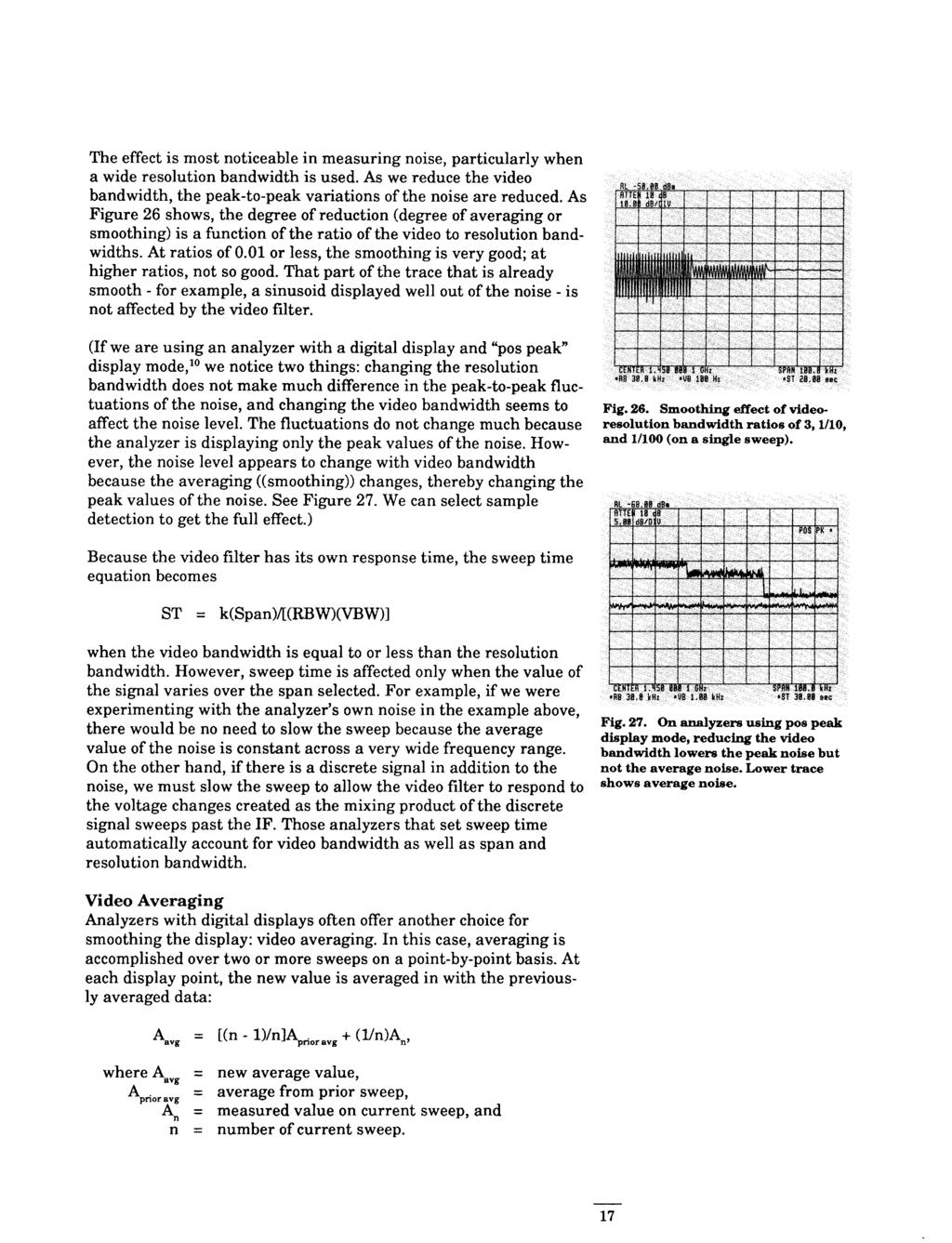
19 What determines the maximum rate at which the envelope of the IF signal can change? The width of the resolution (IF) filter. This bandwidth determines how far apart two input sinusoids can be and, after the mixing process, be within the filter at the same time.8 If we assume a 21.4-MHz final IF and a loo-khz bandwidth, two input signals separated by 100 khz would produce, with the appropriate LO frequency and two or three mixing processes, mixing products of and MHz and so meet the criterion. See Figure 23. The detector must be able to follow the changes in the envelope created by these two signals but not the nominal 21.4 MHz IF signal itself. The envelope detector is what makes the spectrum analyzer a voltmeter. If we duplicate the situation above and have two equalamplitude signals in the passband of the IF at the same time, what would we expect to see on the display? A power meter would indicate a power level 3 db above either signal; that is, the total power of the two. Assuming that the two signals are close enough so that, with the analyzer tuned half way between them, there is negligible attenuation due to the roll-off of the filter, the analyzer display will vary between a value twice the voltage of either (6 db greater) and zero (minus infinity on the log scale). We must remember that the two signals are sine waves (vectors) at different frequencies, and so they continually change in phase with respect to each other. At some time they add exactly in phase; at another, exactly out of phase. So the envelope detector follows the changing amplitude values of the peaks of the signal from the IF chain but not the instantaneous values. And gives the analyzer its voltmeter characteristics. Although the digitally-implemented resolution bandwidths do not have an analog envelope detector, one is simulated for consistency *V!J 0.60 tlhz with the other bandwidths. Fig. 24. Spectrum analyzers display signal plus noise. Display Smoothing Video Filtering Spectrum analyzers display signals plus their own internal noise,g as shown in Figure 24. To reduce the effect of noise on the displayed signal amplitude, we often smooth or average the display, as shown in Figure 25. All HP superheterodyne analyzers include a variable video filter for this purpose. The video filter is a low-pass filter that follows the detector and determines the bandwidth of the video circuits that drive the vertical deflection system of the display. As the cutoff frequency of the video filter is reduced to the point at which it becomes equal to or less than the bandwidth of the selected resolution (IF) filter, the video system can no longer follow the more rapid variations of the envelope of the signal(s).rs 1.18 m ST IBBC passing through the IF chain. The result is an averaging or smoothing of the displayed signal. Fig. 26. Display of Fig. 24 after full smoothing. 16

20

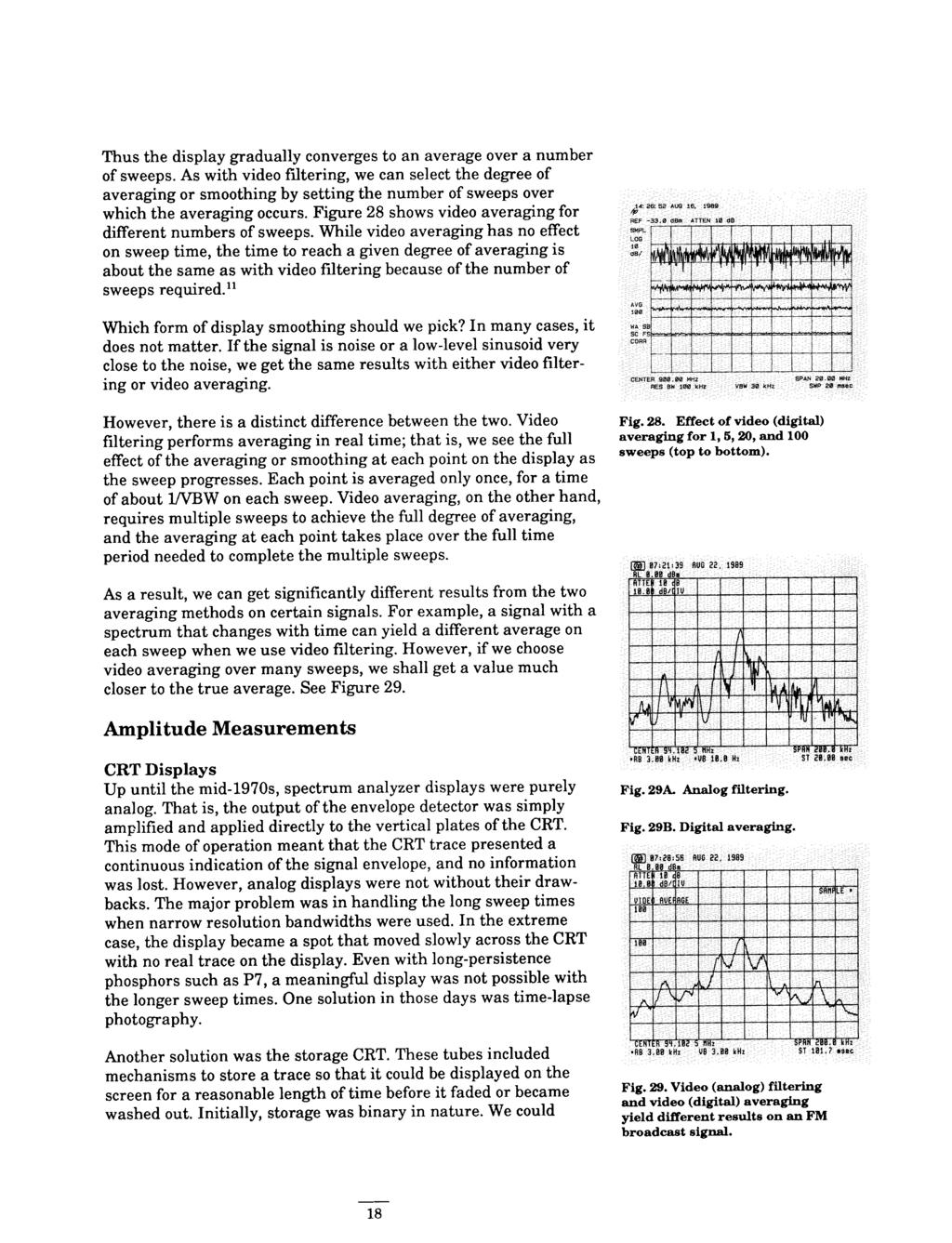
21

22 choose permanent storage, or we could erase the display and start over. Hewlett-Packard pioneered a variable-persistence mode in which we could adjust the fade rate of the display. When properly adjusted, the old trace would just fade out at the point where the new trace was updating the display. The idea was to provide a display that was continuous, had no flicker, and avoided confusing overwrites. The system worked quite well with the correct trade-off between trace intensity and fade rate. The difficulty was that the intensity and the fade rate had to be readjusted for each new measurement situation. When digital circuitry became affordable in the mid-1970s, it was quickly put to use in spectrum analyzers. Once a trace had been digitized and put into memory, it was permanently available for display. It became an easy matter to update the display at a flickerfree rate without blooming or fading. The data in memory was updated at the sweep rate, and since the contents of memory were written to the display at a flicker-free rate, we could follow the updating as the analyzer swept through its selected frequency span just as we could with analog systems. m lsrsl:36 RGG 3, Fig. 30. When digitizing an analog signal, what value should be displayed at each point? Digital Displays But digital systems were not without problems of their own. What value should be displayed? As Figure 30 shows, no matter how many data points we use across the CRT, each point must represent what has occurred over some frequency range and, although we usually do not think in terms of time when dealing with a spectrum analyzer, over some time interval. Let us imagine the situation illustrated in Figure 30: we have a display that contains a single CW signal and otherwise only noise. Also, we have an analog system whose output we wish to display as faithfully as possible using digital techniques Fig. 31. The sample display mode using ten points to display the signal of Figure 30. As a first method, let us simply digitize the instantaneous value of the signal at the end of each interval (also called a cell or bucket). This is the sample mode. To give the trace a continuous look, we design a system that draws vectors between the points. From the conditions of Figure 30, it appears that we get a fairly reasonable display, as shown in Figure 31. Of course, the more points in the trace, the better the replication of the analog signal. The number of points is limited, with 1,000 being the maximum typically offered on any spectrum analyzer. As shown in Figure 32, more points do indeed get us closer to the analog signal. While the sample mode does a good job of indicating the randomness of noise, it is not a good mode for a spectrum analyzer s usual function: analyzing sinusoids. If we were to look at a loo-mhz comb on the HP 71210, we might set it to span from 0 to 22 GHz. Even with 1,000 display points, each point represents a span of 22 GHz, far wider than the maximum ~-MHZ resolution bandwidth. Fig. 32. More points produce a display closer to an analog display. 19

23 As a result, the true amplitude of a comb tooth is shown only if its mixing product happens to fall at the center of the IF when the sample is taken. Figure 33 shows a 5-GHz span with a l-mhz band-width; the comb teeth should be relatively equal in amplitude. Figure 34 shows a 500-MHz span comparing the true comb with the results from the sample mode; only a few points are used to exaggerate the effect. (The sample trace appears shifted to the left because the value is plotted at the beginning of each interval.) One way to insure that all sinusoids are reported is to display the maximum value encountered in each cell. This is the positive-peak display mode, or pos peak. This display mode is illustrated in Figure 35. Figure 36 compares pos peak and sample display modes. Pos peak is the normal or default display mode offered on many spectrum analyzers because it ensures that no sinusoid is missed, regardless of the ratio between resolution bandwidth and cell width. However, unlike sample mode, pos peak does not give a good representation of random noise because it captures the crests of the noise. So spectrum analyzers using the pos peak mode as their primary display mode generally also offer the sample mode as an alternative. Fig. 33. A 6-GHx span of a loo-mhz comb in the sample display mode. The actual comb values are relatively constant over this range. Fig. 34. The actual comb and results of the sample display mode over a 500-MHz span. When resolution bandwidth is narrower than the sample interval, the sample mode can give erroneous results. (The sample trace has only 20 points to exaggerate the effect.) Fig. 35. Pos peak display mode versus actual comb. Fig. 36. Comparison of sample and pos peak display modes. To provide a better visual display of random noise than pos peak and yet avoid the missed-signal problem of the sample mode, the rosenfell display mode is offered on many spectrum analyzers. Rosenfell is not a person s name but rather a description of the algorithm that tests to see if the signal rose and fell within the cell represented by a given data point. Should the signal both rise and fall, as determined by pos-peak and neg-peak detectors, then the algorithm classifies the signal as noise. In that case, an odd-numbered data point indicates the maximum value encountered during its cell. On the other hand, an even-numbered data point indicates the minimum value encountered during its cell. Rosenfell and sample modes are compared in Figure 37. Fig. 37. Comparison of rosenfell and sample display modes. 20

24 What happens when a sinusoidal signal is encountered? We know that as a mixing product is swept past the IF filter, an analyzer traces out the shape of the filter on the display. If the filter shape is spread over many display points, then we encounter a situation in which the displayed signal only rises as the mixing product approaches the center frequency of the filter and only falls as the mixing product moves away from the filter center frequency. In either of these cases, the pos-peak and neg-peak detectors sense an amplitude change in only one direction, and, according to the rosenfell algorithm, the maximum value in each cell is displayed. See Figure 38. What happens when the resolution bandwidth is narrow relative to a cell? If the peak of the response occurs anywhere but at the very end of the cell, the signal will both rise and fall during the cell. If the cell happens to be an odd-numbered one, all is well. The maxi- 1% CHz VB w**t mum value encountered in the cell is simply plotted as the next data point. However, if the cell is even-numbered, then the mini- Fig. 38. When detected signal only mum value in the cell is plotted. Depending on the ratio of resolu- tion bandwidth to cell width, the minimum value can differ from the true peak value (the one we want displayed) by a little or a lot. In the extreme, when the cell is much wider than the resolution bandwidth, the difference between the maximum and minimum values encountered in the cell is the full difference between the peak signal value and the noise. Since the rosenfell algorithm calls for the minimum value to be indicated during an even-numbered cell, the algorithm must include some provision for preserving the maximum value encountered in this cell. To ensure no loss of signals, the pos-peak detector is reset only after the peak value has been used on the display. Otherwise, the peak value is carried over to the next cell. Thus when a signal both rises and falls in an even-numbered cell, and the minimum value is displayed, the pos-peak detector is not reset. The pos-peak value is carried over to the next cell, an odd-numbered cell. During this cell, the pos-peak value is updated only if the signal value exceeds the value carried over. The displayed value, then, is the larger of the held-over value and the maximum value encountered in the new, odd-numbered cell. Only then is the pos-peak detector reset. This process may cause a maximum value to be displayed one data point too far to the right, but the offset is usually only a small percentage of the span. Figure 39 shows what might happen in such a case. A small number of data points exaggerates the effect. rises or falls, as when mixing product sweeps past resolution filter, rosenfell displays maximum values. The rosenfell display mode does a better job of combining noise and discrete spectral components on the display than does pos peak. We get a much better feeling for the noise with rosenfell. However, because it allows only maxima and minima to be displayed, rosenfell does not give us the true randomness of noise as the sample mode does. For noise signals, then, the sample display mode is the best. Fig. 39. Rosenfell when signal peak falls between data points (fewer trace pointa exaggerate the effect). 21

25 HP analyzers that use rosenfell as their default, or normal, display mode also allow selection of the other display modes - pos peak, neg peak, and sample. As we have seen, digital displays distort signals in the process of getting them to the screen. However, the pluses of digital displays greatly outweigh the minuses. Not only can the digital information be stored indefinitely and refreshed on the screen without flicker, blooming, or fade, but once data is in memory, we can add capabilities such as markers and display arithmetic or output data to a computer for analysis or further digital signal processing. Amplitude Accuracy Now that we have our signal displayed on the CRT, let s look at amplitude accuracy. Or, perhaps better, amplitude uncertainty. Most spectrum analyzers these days are specified in terms of both absolute and relative accuracy. However, relative performance affects both, so let us look at those factors affecting relative measurement uncertainty first. Relative Uncertainty When we make relative measurements on an incoming signal, we use some part of the signal as a reference. For example, when we make second-harmonic distortion measurements, we use the fundamental of the signal as our reference. Absolute values do not come into play;12 we are interested only in how the second harmonic differs in amplitude from the fundamental. So what factors come into play? Table I gives us a reasonable shopping list. The range of values given covers a wide variety of spectrum analyzers. For example, frequency response, or flatness, is frequency-range dependent. A low-frequency RF analyzer might have a frequency response of +0.5 db.13 On the other hand, a microwave spectrum analyzer tuning in the 20-GHz range could well have a frequency response in excess of?4 db. Display fidelity covers a variety of factors. Among them are the log amplifier (how true the logarithmic characteristic is), the detector (how linear), and the digitizing circuits (how linear). The CRT itself is not a factor for those analyzers using digital techniques and offering digital markers because the marker information is taken from trace memory, not the CRT. The display fidelity is better over small amplitude differences, so a typical specification for display fidelity might read 0.1 db/db, but no more than the value shown in Table I for large amplitude differences. Table I. Amplitude Uncertainties Relative MB Frequency response 0.54 Display fidelity ARF attenuator AIF attenuator/gain 0.1-l AResolution bandwidth 0.1-l ACRT scaling 0.1-l Absolute Calibrator 0.2-l The remaining items in the table involve control changes made during the course of a measurement. See Figure 40. Because an RF input attenuator must operate over the entire frequency range of the analyzer, its step accuracy, like frequency response, is a function of frequency. At low RF frequencies, we expect the attenuator to be quite good; at 20 GHz, not as good. On the other hand, the IF attenuator (or gain control) should be more accurate because it operates at only one frequency. Another parameter that we might 22

26 change during the course of a measurement is resolution bandwidth. Different filters have different insertion losses. Generally we see the greatest difference when switching between inductorcapacitor (LC) filters, typically used for the wider resolution bandwidths, and crystal filters. Finally, we may wish to change display scaling from, say, 10 db/div to 1 db/div or linear. A factor in measurement uncertainty not covered in the table is impedance mismatch. Analyzers do not have perfect input impedances, nor do most signal sources have ideal output impedances. However, in most cases uncertainty due to mismatch is relatively small. Improving the match of either the source or analyzer reduces uncertainty. Since an analyzer s match is worst with its input attenuator set to 0 db, we should avoid the 0-dB setting if we can. If need be, we can attach a well-matched pad (attenuator) to the analyzer input and so effectively remove mismatch as a factor. 3c/ Fig. 40. Controls that affect r>l/ amplitude accuracy. rl 1 I R.F. IF RES ATTEN Anen/Gain SW Absolute Accuracy The last item in Table I is the calibrator, which gives the spectrum analyzer its absolute calibration. For convenience, calibrators are typically built into today s spectrum analyzers and provide a signal with a specified amplitude at a given frequency. We then rely on the relative accuracy of the analyzer to translate the absolute calibration to other frequencies and amplitudes. Improving Overall Uncertainty If we are looking at measurement uncertainty for the first time, we may well be concerned as we mentally add up the uncertainty figures. And even though we tell ourselves that these are worstcase values and that almost never are all factors at their worst and in the same direction at the same time, still we must add the figures directly if we are to certify the accuracy of a specific measurement. There are some things that we can do to improve the situation. First of all, we should know the specifications for our particular spectrum analyzer. These specifications may be good enough over the range in which we are making our measurement. If not, Table I suggests some opportunities to improve accuracy. Before taking any data, we can step through a measurement to see if any controls can be left unchanged. We might find that a given RF attenuator setting, a given resolution bandwidth, and a given display scaling suffice for the measurement. If so, all uncertainties associated with changing these controls drop out. We may be able to 23

27 trade off IF attenuation against display fidelity, using whichever is more accurate and eliminating the other as an uncertainty factor. We can even get around frequency response if we are willing to go to the trouble of characterizing our particular analyzer.14 The same applies to the calibrator. If we have a more accurate calibrator, or one closer to the frequency of interest, we may wish to use that in lieu of the built-in calibrator. Finally, many analyzers available today have self-calibration routines. These routines generate error coefficients (for example, amplitude changes versus resolution bandwidth) that the analyzer uses later to correct measured data. The smaller values shown in Table I, 0.5 db for display fidelity and 0.1 db for changes in IF attenuation, resolution bandwidth, and display scaling, are based on corrected data. As a result, these self-calibration routines allow us to make good amplitude measurements with a spectrum analyzer and give us more freedom to change controls during the course of a measurement. Sensitivity One of the primary uses of a spectrum analyzer is to search out and measure low-level signals. The ultimate limitation in these measurements is the random noise generated by the spectrum analyzer itself. This noise, generated by the random electron motion throughout the various circuit elements, is amplified by the various gain stages in the analyzer and ultimately appears on the display as a noise signal below which we cannot make measurements. A likely starting point for noise seen on the display is the first stage of gain in the analyzer. This amplifier boosts the noise generated by its input termination plus adds some of its own. As the noise signal passes on through the system, it is typically high enough in amplitude that the noise generated in subsequent gain stages adds only a small amount to the noise power. It is true that the input attenuator and one or more mixers may be between the input connector of a spectrum analyzer and the first stage of gain, and all of these components generate noise. However, the noise that they generate is at or near the absolute minimum of -174 dbm/hz (LTB), the same as at the input termination of the first gain stage, so they do not significantly affect the noise level input to, and amplified by, the first gain stage. While the input attenuator, mixer, and other circuit elements between the input connector and first gain stage have little effect on the actual system noise, they do have a marked effect on the ability of an analyzer to display low-level signals because they attenuate the input signal. That is, they reduce the signal-to-noise ratio and so degrade sensitivity. We can determine sensitivity simply by noting the noise level indicated on the display with no input signal applied. This level is the analyzer s own noise floor. Signals below this level are masked by the noise and cannot be seen or measured. However, the displayed noise floor is not the actual noise level at the input but rather the effective noise level. An analyzer display is calibrated to 24

28 reflect the level of a signal at the analyzer input, so the displayed noise floor represents a fictitious (we have called it an effective) noise floor at the input below which we cannot make measurements. The actual noise level at the input is a function of the input signal. Indeed, noise is sometimes the signal of interest. Like any discrete signal, a noise signal must be above the effective (displayed) noise floor to be measured. The effective input noise floor includes the losses (attenuation) of the input attenuator, mixer(s), etc., prior to the first gain stage. We cannot do anything about the conversion loss of the mixers, but we do have control over the RF input attenuator. By changing the value of input attenuation, we change the attenuation of the input signal and so change the displayed signal-to-noise-floor ratio, the level of the effective noise floor at the input of the analyzer, and the sensitivity. We get the best sensitivity by selecting minimum (zero) RF attenuation. Different analyzers handle the change of input attenuation in different ways. Because the input attenuator has no effect on the actual noise generated in the system, some analyzers simply leave the displayed noise at the same position on the display regardless of the input-attenuator setting. That is, the IF gain remains constant. This being the case, the input attenuator will affect the location of a true input signal on the display. As we increase input attenuation, further attenuating the input signal, the location of the signal on the display goes down while the noise remains stationary. To maintain absolute calibration so that the actual input signal always has the same reading, the analyzer changes the indicated reference level (the value of the top line of the graticule). This design is used in older HP analyzers. In newer HP analyzers, starting with the HP 85688, an internal microprocessor changes the IF gain to offset changes in the input attenuator. Thus, true input signals remain stationary on the display as we change the input attenuator, while the displayed noise moves up and down. In this case, the reference level remains unchanged. See Figures 41 and 42. In either case, we get the best signal-to-noise ratio (sensitivity) by selecting minimum input attenuation. Resolution bandwidth also affects signal-to-noise ratio, or sensitivity. The noise generated in the analyzer is random and has a constant amplitude over a wide frequency range. Since the resolution, or IF, bandwidth filters come after the first gain stage, the total noise power that passes through the filters is determined by the width of the filters. This noise signal is detected and ultimately reaches the display. The random nature of the noise signal causes the displayed level to vary as lo*log(bw.jbw,), where bw 1 = starting resolution bandwidth and bw 2 = ending resolution bandwidth. Fig. 41. Some spectrum analyzers change reference level when RF attenuator is changed, so an input signal moves on the display, but the analyzeis noise does not. Fig. 42. Other analyzers keep reference level constant by changing IF gain, so as RF attenuator is changed, the analyzer s noise moves, but an input signal does not. 25

29 So if we change the resolution bandwidth by a factor of 10, the displayed noise level changes by 10 dbi5, as shown in Figure 43. We get best signal-to-noise ratio, or best sensitivity, using the minimum resolution bandwidth available in our spectrum analyzer. A spectrum analyzer displays signal plus noise, and a low signal-tonoise ratio makes the signal difficult to distinguish. We noted above that the video filter can be used to reduce the amplitude fluctuations of noisy signals while at the same time having no effect on constant signals. Figure 44 shows how the video filter can improve our ability to discern low-level signals. It should be noted that the video filter does not affect the average noise level and so does not, strictly speaking, affect the sensitivity of an analyzer. In summary, we get best sensitivity by selecting the minimum resolution bandwidth and minimum input attenuation. These settings give us best signal-to-noise ratio. We can also select minimum video bandwidth to help us see a signal at or close to the noise level.16 Of course, selecting narrow resolution and video bandwidths does lengthen the sweep time. Noise Figure Many receiver manufacturers specify the performance of their receivers in terms of noise figure rather than sensitivity. As we shall see, the two can be equated. A spectrum analyzer is a receiver, and we shall examine noise figure on the basis of a sinusoidal input. IR 9.s *.* Fig. 43. Displayed noise level changes as lo*log(bw,/bw,). Noise figure can be defined as the degradation of signal-to-noise ratio as a signal passes through a device, a spectrum analyzer in our case. We can express noise figure as F = (S,/N,Y(So/N,,), where F = noise figure as power ratio, Si = input signal power, Ni = true input noise power, so = output signal power, and No = output noise power. If we examine this expression, we can simplify it for our spectrum analyzer. First of all, the output signal is the input signal times the gain of the analyzer. Second, the gain of our analyzer is unity because the signal level at the output (indicated on the display) is the same as the level at the input (input connector). So our expression, after substitution, cancellation, and rearrangement, becomes Fig. 44. Video filtering makes low- 1 eve1 signals more discernable. (The average trace was offset for visibility.) F = No/N,. This expression tells us that all we need to do to determine the noise figure is compare the noise level as read on the display to the true (not the effective) noise level at the input connector. Noise figure is usually expressed in terms of db, or NF = lo*log(f) = 10*log(NO) - lo*log(n,). 26

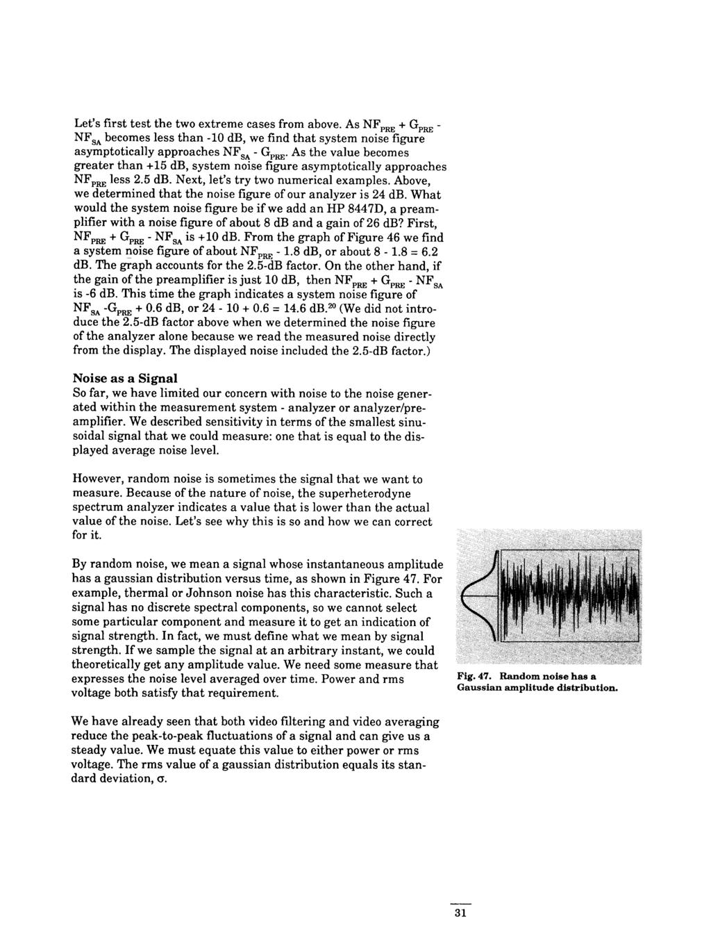
30 We use the true noise level at the input rather than the effective noise level because our input signal-to-noise ratio was based on the true noise. Now we can obtain the true noise at the input simply by terminating the input in 50 ohms. The input noise level then becomes N, = ktb, where k = Boltzmann s constant, T = absolute temperature in degrees kelvin, and B = bandwidth. At room temperature and for a l-hz bandwidth, ktb = -174 dbm. We know that the displayed level of noise on the analyzer changes with bandwidth. So all we need to do to determine the noise figure of our spectrum analyzer is to measure the noise power in some bandwidth, calculate the noise power that we would have measured in a l-hz bandwidth using lo*log(bwjbw,), and compare that to -174 dbm. For example, if we measured -110 dbm in a lo-khz resolution bandwidth, we would get NF = (measured noise),m,, - lo*log(rbw/l) - ktb,_, = -110 dbm - 10*1og(10,000/1) - (-174 dbm) = = 24 db. Noise figure is independent of bandwidth17. Had we selected a different resolution bandwidth, our results would have been exactly the same. For example, had we chosen a l-khz resolution bandwidth, the measured noise would have been -120 dbm and lo*log(rbw/l) would have been 30. Combining all terms would have given = 24 db, the same noise figure as above. The 24-dB noise figure in our example tells us that a sinusoidal signal must be 24 db above ktb to be equal to the average displayed noise on this particular analyzer. Thus we can use noise figure to determine sensitivity for a given bandwidth or to compare sensitivities of different analyzers on the same bandwidth.18 Preamplifiers One reason for introducing noise figure is that it helps us determine how much benefit we can derive from the use of a preamplifier. A 24-dB noise figure, while good for a spectrum analyzer, is not so good for a dedicated receiver. However, by placing an appropriate preamplifier in front of the spectrum analyzer, we can obtain a system (preamplifier/spectrum analyzer) noise figure that is lower than that of the spectrum analyzer alone. To the extent that we lower the noise figure, we also improve the system sensitivity. 27

31

32 the preamplifier less 2.5 db, or 5.5 db. In a lo-khz resolution bandwidth our preamplifier/analyzer system has a sensitivity of ktb,_, + lo*log(rbw/ll + NF,,, = -174 dbm + 40 db db = dbm. This is an improvement of 18.5 db over the -110 dbm noise floor without the preamplifier. Is there any drawback to using this preamplifier? That depends upon our ultimate measurement objective. If we want the best sensitivity but no loss of measurement range, then this preamplitier is not the right choice. Figure 45 illustrates this point. A spectrum analyzer with a 24-dB noise figure will have an average displayed noise level of -110 dbm in a lo-khz resolution bandwidth. If the l-db compression pointlg for that analyzer is -10 dbm, the measurement range is 100 db. When we connect the preamplifier, we must reduce the maximum input to the system by the gain of the pre-amplifier to -46 dbm. However, when we connect the preamplifier, the noise as displayed on the CRT will rise by about 17.5 db because the noise power out of the preamplifier is that much higher than the analyzer s own noise floor, even after accounting for the 2.5-dB factor. It is from this higher noise level that we now subtract the gain of the preamplifier. With the preamplifier in place, our measurement range is 82.5 db, 17.5 db less than without the preamplifier. The loss in measurement range equals the change in the displayed noise when the preamplifier is connected. -10 dbm 1OOdB Spa&urn Analyzer Range d&n/l0 khz Spectrum Analyzer t ds csmprassion Avg. notes on CRT Spectrum Analyzer & Preamplifier ds System Range Q Pm } -46 dsm System 1 ds cdmprsssion Avg. noise on CRT System sensitivity Fig. 45. If the displayed noise goes up when a preamplifier is connected, measurement range is diminished by the amount the noise changes. Is there a preamplifier that will give us better sensitivity without costing us measurement range? Yes. But it must meet the second of the above criteria; that is, the sum of its gain and noise figure must be at least 10 db less than the noise figure of the spectrum analyzer. In this case the displayed noise floor will not change noticeably when we connect the preamplifier, so although we shift the whole measurement range down by the gain of the preamplifier, we end up with the same overall range that we started with. 29

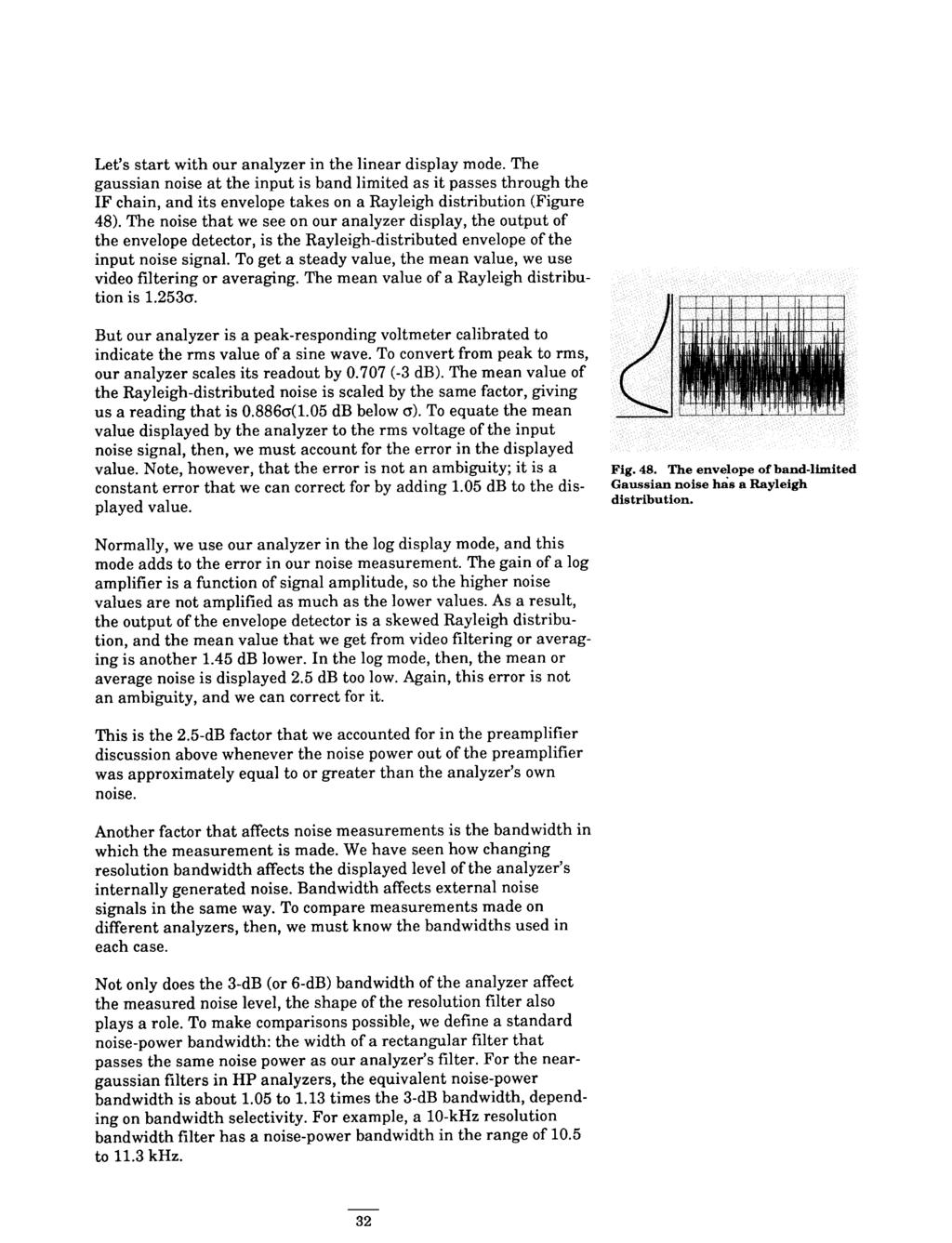
33

34

35

36 If we use 10*log(bwz/bw,l to adjust the displayed noise level to what we would have measured in a noise power bandwidth of the same numeric value as our 3-dB bandwidth, we find that the adjustment varies from 10*1og(10,000/10,500) = db to 10*1og(10,000/11,300) = db. In other words, if we subtract something between 0.21 and 0.53 db from the indicated noise level, we shall have the noise level in a noise-power bandwidth that is convenient for computations. Let s consider all three factors and calculate a total correction: Rayleigh distribution (linear mode): 1.05 db log amplifier (log mode): 1.45 db 3-dB/noise power bandwidths: -0.5 db total correction: 2.0 db Here we use -0.5 db as a reasonable compromise for the bandwidth correction. The total correction is thus a convenient value. Many of today s microprocessor-controlled analyzers allow us to activate a noise marker. When we do so, the microprocessor switches the analyzer into the sample display mode, computes the mean value of the 32 display points about the marker, adds the above 2-dB amplitude correction, normalizes the value to a l-hz noise-power bandwidth, and displays the normalized value. The analyzer does the hard part. It is reasonably easy to convert the noise-marker value to other bandwidths. For example, if we want to know the total noise in a ~-MHZ communication channel, we add 66 db to the noise-marker value (60 db for the 1,000,000/1 and another 6 db for the additional factor of four). Preamplifier for Noise Measurements Since noise signals are typically low-level signals, we often need a preamplifier to have sufficient sensitivity to measure them. However, we must recalculate sensitivity of our analyzer first. Above, we defined sensitivity as the level of a sinusoidal signal that is equal to the displayed average noise floor. Since the analyzer is calibrated to show the proper amplitude of a sinusoid, no correction for the signal was needed. But noise is displayed 2.5 db too low, so an input noise signal must be 2.5 db above the analyzer s displayed noise floor to be at the same level by the time it reaches the display. The input and internal noise signals add to raise the displayed noise by 3 db, a factor of two in power. So we can define the noise figure of our analyzer for a noise signal as NFB,,, = (noise floor)dbmm, - lo*log(rbw/l) - ktb,_, db. 33

37 If we use the same noise floor as above, -110 dbm in a lo-khz resolution bandwidth, we get NF,, = -110 dbm - 10*1og(10,000/1)- (174 dbm)+2.5 db = 26.5 db. As was the case for a sinusoidal signal, NF,,, is independent of resolution bandwidth and tells us how far above ktb a noise signal must be to be equal to the noise floor of our analyzer. When we add a preamplifier to our analyzer, the system noise figure and sensitivity improve. However, we have accounted for the 2.5-dB factor in our definition of NF,,, so the graph of system noise figure becomes that of Figure 49. We determine system noise figure for noise the same way that we did for a sinusoidal signal above. NFwNjGp+ 3 db NFpm + 3 db Fig. 49. signals. System noise figure for System Noise FigureWI NFw, jgpre+ 2 db NFp, + 2 db NFw,,).Gm+ 1 db NFp,e + 1 d8 NFSA(NjGpe lo NFpe NFp. + Gpe-NFwNj NW Dynamic Range Definition Dynamic range is generally thought of as the ability of an analyzer to measure harmonically related signals and the interaction of two or more signals; for example, to measure second- or third-harmonic distortion or third-order intermodulation. In dealing with such measurements, remember that the input mixer of a spectrum analyzer is a non-linear device and so always generates distortion of its own. The mixer is non-linear for a reason. It must be nonlinear to translate an input signal to the desired IF. But the unwanted distortion products generated in the mixer fall at the same frequencies as do the distortion products we wish to measure on the input signal. So we might define dynamic range in this way: it is the ratio, expressed in db, of the largest to the smallest signals simultaneously present at the input of the spectrum analyzer that allows measurement of the smaller signal to a given degree of uncertainty. Notice that accuracy of the measurement is part of the definition. We shall see how both internally generated noise and distortion affect accuracy below. 34

38 Dynamic Range versus Internal Distortion To determine dynamic range versus distortion, we must first determine just how our input mixer behaves. Most analyzers, particularly those utilizing harmonic mixing to extend their tuning range,21 use diode mixers. (Other types of mixers would behave similarly.) The current through an ideal diode can be expressed as i = IS(evkT - 11, where q = electronic charge, v = instantaneous voltage, k = Boltzmann s constant, and T = temperature in degrees Kelvin. We can expand this expression into a power series i = J(k,v + k2v2 + k3v3 +...). where k, = q/kt k, = ki2/2!, k, = ki3/3!, etc. Let s now apply two signals to the mixer. One will be the input signal that we wish to analyze; the other, the local oscillator signal necessary to create the IF: v = V,,sin(w,,t) + V,sin(w,t). If we go through the mathematics, we arrive at the desired mixing product that, with the correct LO frequency, equals the IF: k2vlov,cd(w,, - wilti. A k,v,ov,cos[(w,, + wilt1 term is also generated, but in our discussion of the tuning equation, we found that we want the LO to be above the IF, so (wlo + wi) is also always above the IF. With a constant LO level, the mixer output is linearly related to the input signal level. For all practical purposes, this is true as long as the input signal is more than 15 to 20 db below the level of the LO. There are also terms involving harmonics of the input signal: (3k~4lV,oV,2sin(w,, - 2w,)t, (k,/8)v,,v,3sin(w,o - 3w,)t, etc. These terms tell us that dynamic range due to internal distortion is a function of the input signal level at the input mixer. Let s see how this works, using as our definition of dynamic range the difference in db between the fundamental tone and the internally generated distortion. 35

39 The argument of the sine in the first term includes 2w1, so it represents the second harmonic of the input signal. The level of this second harmonic is a function of the square of the voltage of the fundamental, Vi2. This fact tells us that for every db that we drop the level of the fundamental at the input mixer, the internally generated second harmonic drops by 2 db. See Figure 50. The second term includes 3wl, the third harmonic, and the cube of the input-signal voltage, V,3. So a l-db change in the fundamental at the input mixer changes the internally generated third harmonic by 3 db. 2AdB 3AdB AdB I hdb Fig. 50. Changing the level of fundamental tone (w) or tones (w,, WJ at the mixer affects internally generated distortion. 3AdB 3AdB i W 2w 3W 2w1-w2 Wl w2 2w2-w 1 Distortion is often described by its order. The order can be determined by noting the coefficient associated with the signal frequency or the exponent associated with the signal amplitude. Thus secondharmonic distortion is second order and third harmonic distortion is third order. The order also indicates the change in internally generated distortion relative to the change in the fundamental tone that created it. Now let us add a second input signal: v = V,,sin(w,ot) + V,sin(w,t) + V,sin(w,t). This time when we go through the math to find internally generated distortion, in addition to harmonic distortion, we get (k(8wlov,2v2cos[w,o - (2w, - w,llt, (k,/8)vlov,v22cos[w,o - (2w, - w,)lt, etc. These represent intermodulation distortion, the interaction of the two input signals with each other. The lower distortion product, 2w, - w2, falls below wr by a frequency equal to the difference between the two fundamental tones, w2 - wi. The higher distortion product, 2w, - wr, falls above wp by the same frequency. See Figure 50. Once again, dynamic range is a function of the level at the input mixer. The internally generated distortion changes as the product of V,2 and V, in the first case, of V, and V22 in the second. If V, and V, have the same amplitude, the usual case when testing for distor- 36

40 tion, we can treat their products as cubed terms (VI3 or VZ3). Thus, for every db that we simultaneously change the level of the two input signals, there is a 3-dB change in the distortion components as shown in Figure 50. This is the same degree of change that we saw for third harmonic distortion above. And in fact, this, too, is third-order distortion. In this case, we can determine the degree of distortion by summing the coefficients of w1 and w2 or the exponents of V, and V,. All this says that dynamic range depends upon the signal level at the mixer. How do we know what level we need at the mixer for a particular measurement? Many analyzer data sheets now include graphs to tell us how dynamic range varies. However, if no graph is provided, we can draw our own. We do need a starting point, and this we must get from the data sheet. We shall look at second-order distortion first. Let s assume the data sheet says that second-harmonic distortion is 70 db down for a signal -40 dbm at the mixer. Because distortion is a relative measurement, and, at least for the moment, we are calling our dynamic range the difference in db between fundamental tone or tones and the internally generated distortion, we have our starting point. Internally generated second-order distortion is 70 db down, so we can measure distortion down 70 db. We plot that point on a graph whose axes are labeled distortion (dbc) versus level at the mixer (level at the input connector minus the input-attenuator setting). See Figure 51. What happens if the level at the mixer drops to -50 dbm? As noted above (Figure 501, for every db change in the level of the fundamental at the mixer there is a 2-dB change in the internally generated second harmonic. But for measurement purposes, we are only interested in the relative change, that is, in what happened to our measurement range. In this case, for every db that the fundamental changes at the mixer, our measurement range aiso changes by 1 db. In our second-harmonic example, then, when the level at the mixer changes from -40 to -50 dbm, the internal distortion, and thus our measurement range, changes from -70 to -80 dbc. In fact, these points fall on a line with a slope of 1 that describes the dynamic range for any input level at the mixer. s 8 Ol -10 TOI I lo Mixer Level (dbm) Fig. 51. Dynamic range versus distortion and noise. We can construct a similar line for third-order distortion. For example, a data sheet might say third-order distortion is -70 dbc for a level of -30 dbm at this mixer. Again, this is our starting point, and we would plot the point shown in Figure 51. If we now drop the level at the mixer to -40 dbm, what happens? Referring again to Figure 50, we see that both third-harmonic distortion and thirdorder inter-modulation distortion fall by 3 db for every db that the fundamental tone or tones fall. Again it is the difference that is important. If the level at the mixer changes from -30 to -40 dbm, the difference between fundamental tone or tones and internally generated distortion changes by 20 db. So the internal distortion is -90 dbc. These two points fall on a line having a slope of 2, giving us the third-order performance for any level at the mixer. 37

41

42 of -40 dbm at the mixer, it is 70 db above the average noise, so we have 70 db signal-to-noise ratio. For every db that we reduce the signal level at the mixer, we lose 1 db of signal-to-noise ratio. Our noise curve is a straight line having a slope of -1, as shown in Figure 51. Under what conditions, then, do we get the best dynamic range? Without regard to measurement accuracy, it would be at the intersection of the appropriate distortion curve and the noise curve. Figure 51 tells us that our maximum dynamic range for secondorder distortion is 70 db; for third-order distortion, 77 db. Figure 51 shows the dynamic range for one resolution bandwidth. We certainly can improve dynamic range by narrowing the resolution bandwidth, but there is not a one-to-one correspondence between the lowered noise floor and the improvement in dynamic range. For second-order distortion the improvement is one half the change in the noise floor; for third-order distortion, two thirds the change in the noise floor. See Figure 52. The final factor in dynamic range is the phase noise on our spectrum analyzer LO, and this affects only third-order distortion measurements. For example, suppose we are making a two-tone, third-order distortion measurement on an amplifier, and our test tones are separated by 10 khz. The third-order distortion components will be separated from the test tones by 10 khz also. For this measurement we might find ourselves using a 1-kHz resolution bandwidth. Referring to Figure 52 and allowing for a lo-db decrease in the noise curve, we would find a maximum dynamic range of about 84 db. However, what happens if our phase noise at a lo-khz offset is only -75 dbc? Then 75 db becomes the ultimate limit of dynamic range for this measurement, as shown in Fig. 53. In summary, the dynamic range of a spectrum analyzer is limited by three factors: the distortion performance of the input mixer, the broadband noise floor (sensitivity) of the system, and the phase noise of the local oscillator. Ol -10,-50 8 P I. Noise / \ (10 khz BW) lo Mxer Level (dbm) Fig. 52. Reducing resolution bandwidth improves dynamic range. 1 / 3 rd O&Jr lo Mixer Level (dbm) Fig. 53. Phase noise can limit thirdorder intermodulation tests. Dynamic Range versus Measurement Uncertainty In our previous discussion of amplitude accuracy, we included only those items listed in Table I plus mismatch. We did not cover the possibility of an internally generated distortion product (a sinusoid) being at the same frequency as an external signal that we wished to measure. However, internally generated distortion components fall at exactly the same frequencies as the distortion components we wish to measure on external signals. The problem is that we have no way of knowing the phase relationship between the external and internal signals. So we can only determine a potential range of uncertainty: Uncertainty (in db) = 2O*log(l+ 10dno), where d = difference in db between larger and smaller sinusoid (a negative number). 39

43 See Figure 54. For example, if we set up conditions such that the internally generated distortion is equal in amplitude to the distortion on the incoming signal, the error in the measurement could range from +6 db (the two signals exactly in phase) to -infinity (the two signals exactly out of phase and so cancelling). Such uncertainty is unacceptable in most cases. If we put a limit of 1 db on the measurement uncertainty, Figure 54 shows us that the internally generated distortion product must be about 18 db below the distortion product that we wish to measure. To draw dynamic-range curves for second- and third-order measurements with no more than 1 db of measurement error, we must then offset the curves of Figure 51 by 18 db as shown in Figure 55. Next let s look at uncertainty due to low signal-to-noise ratio. The distortion components we wish to measure are, we hope, low-level signals, and often they are at or very close to the noise level of our spectrum analyzer. In such cases we often use the video filter to make these low-level signals more discernable. Figure 56 shows the error in displayed signal level as a function of displayed signal-tonoise for a typical spectrum analyzer. Note that the error is only in one direction, so we could correct for it. However, we usually do not. So for our dynamic-range measurement, let s accept a 0.5-dB error due to noise and offset the noise curve in our dynamic-range chart by 5 db as shown in Figure 55. Where the distortion and noise curves intersect, the maximum error possible would be less than 1.5 db. Let s see what happened to our dynamic range as a result of our concern with measurement error. As Figure 55 shows, secondorder-distortion dynamic range changes from 70 to 56.5 db, a change of 11.5 db. This is one half the total offsets for the two curves (18 db for distortion; 5 db for noise). Third-order distortion changes from 77 db to about 68 db for a change of about 9 db. In this case the change is one third of the 1%dB offset for the distortion curve plus two thirds of the 5-dB offset for the noise curve. Mixer Compression In our discussion of dynamic range, we did not concern ourselves with how accurately the larger tone is displayed, even on a relative basis. As we raise the level of a sinusoidal input signal, eventually the level at the input mixer becomes so high that the desired output mixing product no longer changes linearly with respect to the input signal. The mixer is in saturation, and the displayed signal amplitude is too low. Saturation is gradual rather than sudden. To help us stay away from the saturation condition, the 0.5-dB or 1-dB compression point is usually specified. A mixer level of -10 to -5 dbm is typical. Thus we can determine what input attenuator setting to use for accurate measurement of high-level signals.22 Max Error W Fig. 54. Uncertainty versus difference in amplitude between two sinusoids at the same frequency. B Q I0 Mixer Level (dbm) Fig. 56. Dynamic range for 1.5-dB maximum error db 4.0 d0-2.0 d! db 4OdB 6.0 d0 9.0 db Oiqlplayed 6/N (de) Fig. 56. Error in displayed signal amplitude due to noise. 40

44 Actually, there are three different methods of evaluating compression. The traditional method, called CW compression, measures the change in gain of a device (amplifier or mixer or system) as the input signal power is swept upward. This method is the one just described. Note that the CW compression point is considerably higher than the levels for the fundamentals indicated above for even moderate dynamic range. So we were correct in not concerning ourselves with the possibility of compression of the larger signal(s). A second method, called two-tone compression, measures the change in system gain for a small signal while the power of a larger signal is swept upward. Two-tone compression applies to the measurement of multiple CW signals, such as sidebands and independent signals. The threshold of compression of this method is usually a few db lower than that of the CW method. A final method, called pulse compression, measures the change in system gain to a narrow (broadband) RF pulse while the power of the pulse is swept upward. When measuring pulses, we often use a resolution bandwidth much narrower than the bandwidth of the pulse, so our analyzer displays the signal level well below the peak pulse power.= As a result, we could be unaware of the fact that the total signal power is above the mixer compression threshold. A high threshold improves signal-to-noise ratio for high-power, ultranarrow or widely chirped pulses. The threshold is about 12 db higher than for two-tone compression in the HP 856OA, 8561A/B, and 8562ALEVC analyzers. Nevertheless, because different compression mechanisms affect CW, two-tone, and pulse compression differently, any of the compression thresholds can be lower than any other. Display Range and Measurement Range There are two additional ranges that are often confused with dynamic range: display range and measurement range. Display range, often called display dynamic range, refers to the calibrated amplitude range of the CRT display. For example, a display with eight divisions would seem to have an 80-dB display range when we select 10 db per division. However, in most cases, as with HP, the bottom division is not calibrated. The bottom line of the graticule represents a signal amplitude of zero, so the bottom division of the display covers the range from -70 db to infinity relative to the reference level (top line)24. The bottom division of ten-division displays are also typically uncalibrated. Another factor is the range of the log amplifier. Typical ranges are 70 and 90 db for analyzers with eight and ten divisions, respectively. Some analyzers do have log amplifiers, or use autoranging, to utilize the full 10 divisions of their displays. The HP 8560A and 8561B use a combination of digital signal processing and autoranging for a full loo-db display when we select one of the digitally-implemented resolution bandwidths (10, 30, 100 Hz). 41

45 The question is, can the full display range be used? From the discussion of dynamic range above, we know that the answer is generally yes. In fact, dynamic range often exceeds display range or log amplifier range. What then? To bring the smaller signals into the calibrated area of the display, we must increase IF gain. But in so doing, we move the larger signals off the top of the display, above the reference level. In HP analyzers, we can move signals at least 20 db above the reference level without affecting the accuracy with which the smaller signals are displayed. So we can indeed take advantage of the full dynamic range of an analyzer even when the dynamic range exceeds the display range. Measurement range is the ratio of the largest to the smallest signal that can be measured under any circumstances. The upper limit is determined by the maximum safe input level, +30 dbm (1 watt) for most analyzers. These analyzers have input attenuators settable to 60 or 70 db, so we can reduce +30-dBm signals to levels well below the compression point of the input mixer and measure them accurately. Sensitivity sets the other end of the range. Depending on the minimum resolution bandwidth of the particular analyzer, sensitivity typically ranges from -115 to -135 dbm. Measurement range, then, can vary from 145 to 160 db. Of course, we cannot view a -135 dbm signal while a +30 dbm signal is also present at the input. Frequency Measurements So far, we have focused almost exclusively on amplitude measurements. What about frequency measurements? Up until the late 197Os, absolute frequency uncertainty was measured in megahertz because the first LO was a high-frequency oscillator operating above the RF range of the analyzer, and there was no attempt to tie the LO to a more accurate reference oscillator. (An exception was the HP 8580, an automatic spectrum analyzer based on the HP 8555A, in which an external synthesizer was substituted for the internal LO. However, the cost of the system prevented its use as a general-pur-pose analyzer.) Many analyzers of this type are still available and in general use. Examples are the HP 8590 and Absolute frequency uncertainty of even many megahertz is not a hinderance in many cases. For example, many times we are measuring an isolated signal. Or we need just enough accuracy to be able to identify the signal of interest among other signals. Absolute frequency is often listed under the Frequency Readout Accuracy specification and refers to center frequency and, for analyzers with microprocessors and digital displays, start, stop, and marker frequencies. More important, usually, is relative frequency uncertainty. How far apart are spectral components? What is the modulation frequency? Here the span accuracy comes into play. For HP analyzers, span accuracy generally means the uncertainty in the indicated separation of any two spectral components on the display. For example, suppose span accuracy is 3% and we have two signal separated by 42

46 two divisions on a l-mhz span (100 khz per division). The uncertainty of the signal separation would be 6 khz. The uncertainty would be the same if we used delta markers and the delta reading was 200 khz. Span accuracy can be used to improve low-frequency accuracy. How would we tune to a loo-khz signal on an analyzer having 5 MHz frequency uncertainty? We can use the LO feedthrough (the response created when the first LO sweeps past the first IF) as a zero-frequency marker and the span accuracy to locate the signal. The LO feedthrough indicates 0 Hz with no error, and we can place it at the left side of the display graticule with a span of 200 khz. Again assuming 3% span accuracy, our signal should appear at the center of the display +O. 15 divisions. With the introduction of the HP 8568A in 1978, counter-like frequency accuracy became available in a general-purpose spectrum analyzer. A low-drift, ovenized crystal oscillator was added as a reference for all of the LOS in the instrument. Over the years, crystal reference oscillators, some ovenized, some not, have been added to analyzers in all cost ranges. A comment on stabilized oscillators. If we use the broadest definition of indirect synthesis, that the frequency of the oscillator in question is in some way determined by a reference oscillator, then the actual technique used is irrelevant. Phase lock, frequency discrimination, counter lock all fall within this definition of indirect synthesis. What we really care about is the effect on frequency accuracy (and drift). A typical readout accuracy might be stated as follows: +[(freq readout x freq ref error) + A% of span+ B% of RBW + C Hz]. Note that we cannot determine an exact frequency error unless we know something about the frequency reference. In some cases we are given an annual aging rate (for example, f2 x 10.Vyear); in others, aging over a shorter period (for example, *5 x lo-lo/day). In addition, we need to know when the oscillator was last adjusted and how close it was set to its nominal frequency (usually 10 MHz). Other factors that we often overlook when we think about frequency accuracy are whether or not the instrument was unplugged from the power line before we use it (some reference oscillators require 72 hours to reach their specified drift rate) and the temperature coefficient (it can be worse than the drift rate). In short, there are a number of factors to consider before we can determine frequency uncertainty. In a factory setting there is often an in-house frequency standard available that is traceable to a national standard. Most analyzers with internal reference oscillators allow substitution of an external reference. The frequency reference error in the above expression then becomes that of the in-house standard. 43

47 When making measurements in the field, we typically want to turn our analyzer on, complete our task, and move on as quickly as possible. It is helpful to know how the reference in our analyzer behaves under short warmup conditions. For the HP 8560 series of portable spectrum analyzers, specifications for the standard reference give performance after a five-minute warmup; specifications for the precision frequency reference give performance for both five- and fifteen-minute warmup. Most analyzers with digital displays include markers. When a single marker is activated, it gives us absolute frequency (as well as amplitude). However, the indicated frequency of the marker is a function of the frequency calibration of the display and the location of the marker on the display. To get best frequency accuracy, then, we must be careful to place the marker exactly at the peak of the response to a spectral component. If we place the marker at some other point on the response, we shall get a different frequency reading. For the best accuracy, we may narrow the span and resolution bandwidth to minimize their effects and to make it easier to place the marker at the peak of the response. Many analyzers that have markers include an internal counter schemes that eliminate the effects of span and resolution bandwidth on frequency accuracy. The counter does not count the input signal directly but instead counts the IF signal and perhaps one or more of the LOS, and the microprocessor computes the frequency of the input signal. A minimum signal-to-noise ratio is required to eliminate noise as a factor in the count. But counting the signal in the IF also eliminates the need to place the marker at the exact peak of the signal response on the display. Anywhere sufficiently out of the noise will do. Marker count accuracy might be stated as: *[(marker freq x freq ref error) + counter resolution + A Hz]. We must still deal with the frequency reference error as above. Counter resolution refers to the least significant digit in the counter readout, a factor here just as with any digital counter. Some analyzers allow the counter mode to be used with delta markers. In that case, the effects of counter resolution and the fixed frequency would be doubled. Summary In this chapter we have described the RF superheterodyne spectrum analyzer. We went through the block diagram and noted how the various sections affect our ability to make measurements. We looked at amplitude accuracy, sensitivity, and dynamic range, and ended with a discussion of frequency measurements. In the next chapter we shall see how we might extend the frequency range to enable us to analyze microwave signals.alyze microwave signals. 44

48 Footnotes (Chapter 2) Not exactly true for analyzers with digital displays. However, describing the ramp as if it did directly control the CRT beam simplifies the discussion, so we shall continue to do so. See CRT Displays (page 18). *See Amplitude Accuracy (page 21). In the text we shall mund off some of the frequency values for simplicity although the exact values are shown in the figures. If you experiment with resolution on a spectrum analyzer that has an analog display or one that has a digital display and msenfell display mode, use enough video filtering to create a smooth trace; otherwise, there will be a smearing as the two signals interact. While the smeared trace certainly indicates the presence of more than one signal, it is difficult to determine the amplitudes of the individual signals fmm that trace. Spectrum analyzers with digital displays and positive peak as their normal display mode may not show the smearing effect. You can observe the smearing by selecting the alternate sample display mode. 6Also see Sweep Time (page 13). OThe effect is the same for the broadband noise floor (or any broadband noise signal). See Sensitivity (page 24). A signal whose frequency range extends from zem (dc) to some upper frequency determined by the circuit elements. 8For this discussion, we assume that the filter is perfectly rectangular. %Jee Dynamic Range versus Measurement Uncertainty (page 39). See Digital Displays (page 19). Most analyzers automatically switch to a sample display mode when video averaging is selected. See Digital Displays (page 19) for potential loss of signal information in the sample mode. uexcept to the extent that dynamic range is affected. See Dynamic Range (page 34). 13Generally, frequency response is defined as half the peak-to-peak response. Should we do so, then mismatch may become a more significant factor. IsNot always true for the analyzer s own noise because of the way IF step gain and filter poles are distributed throughout the IF chain. However, the relationship does hold true when the noise is the external signal being measured. rbfor the effect of noise on accuracy, see Measurement Uncertainty under dynamic range. This may not be precisely true for a given analyzer because of the way resolution filter sections and gain are distributed in the IF chain. lethe noise figure computed in this manner cannot be compared directly to that of a receiver or amplifier because the measured noise term in the equation understates the actual noise by 2.5 db. See Noise as a Signal (page 31). lesee Mixer Compression (page 40). * For more details on noise figure, see HP Application Note 57-1, Fundamentals of RF and Microwave Noise Figure Measurements. Wee Chapter 3 (page 46). *2Many analyzers internally control the combined settings of the input attenuator and IF gain so that a cw as high as the compression level at the input mixer creates a deflection above the top line of the graticule. Thus we cannot make incorrect measumments inadvertently. *%See HP Application Note 150-2, Pulsed RF. l Because of the internally generated noise, analyzers always display some signal above the bottom line of the graticule on 10 db/div and higher scale factors. 45

49 Chapter 3 Extending the Frequency Range Harmonic Mixing In Chapter 2 we described a single-range spectrum analyzer that tunes to 2.9 GHz. Now we wish to tune higher in frequency, perhaps to 22 GHz. The most economical way to achieve such an extended range is to use harmonic mixing. But let us take one step at a time. In developing our tuning equation in Chapter 2, we found that we needed the low-pass filter of Figure 7 to prevent higher-frequency signals from reaching the mixer. The result was a uniquely-responding, single-band analyzer that tuned to 2.9 GHz. Now we wish to observe and measure higher-frequency signals, so we must remove the low-pass filter Gtiz Fig. 57. Switching arrangement to 21,4 MHz provide a high IF for the low band and a low IF for the high bands GHz To CRT Another factor that we explored in developing the tuning equation was the choice of LO and intermediate frequencies. We decided that the IF should not be within the band of interest because it created a hole in our tuning range in which we could not make measurements. So we chose 3.6 GHz, moving the IF above the highest tuning range of interest (2.9 GHz). Since our new tuning range will be above 2.9 GHz, it seems logical to move the new IF to a frequency below 2.9 GHz. A typical first IF for these higherfrequency ranges in HP spectrum analyzers is MHz. We shall use this frequency in our examples. In summary, for the low band, up to 2.9 GHz, our first IF is 3.6 GHz. For the upper frequency bands, we must switch to a first IF of MHz. Note that in Figure 10 the second IF is MHz, so all we need to do when we wish to tune to the higher ranges is bypass the first IF, as shown in Figure 57. In Chapter 2 we used a mathematical approach to conclude that we needed a low-pass filter. As we shall see, things become more complex in the situation here, so we shall use a graphical approach as an easier method to see what is happening. The low band is the simpler case, so we shall start with that. In all of our graphs, we shall plot the LO frequency along the horizontal axis and signal frequency along the vertical axis, as shown in Figure 58. Since we know that we get a mixing product equal to the IF (and therefore a response on the display) whenever the input signal differs from the 46

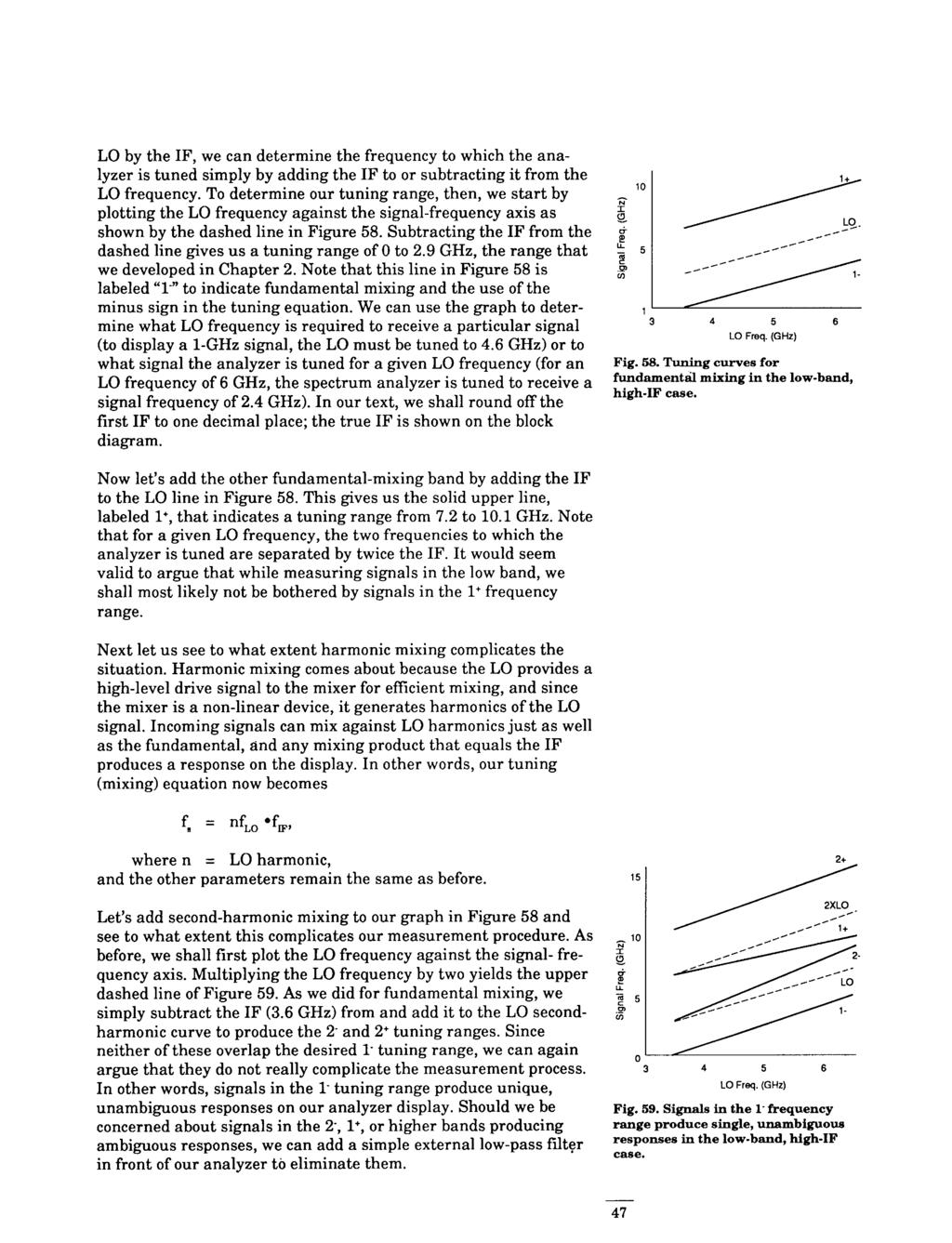
50

51 I he situation is considerably different for the high-band, low-if case. As before, we shall start by plotting the LO fundamental against the signal-frequency axis and then add and subtract the IF, producing the results shown in Figure 60. Note that the l- and 1 tuning ranges are much closer together, and in fact overlap, because the IF is a much lower frequency, MHz in this case. Does the close spacing of the tuning ranges complicate the measurement process? Yes and no. First of all, our system can be calibrated for only one tuning range at a time. In this case, we would choose the l- tuning to give us a low-end frequency of 2.7 GHz so that we have some overlap with the 2.9 GHz upper end of our lowband tuning range. So what are we likely to see on the display? If we enter the graph at an LO frequency of 5 GHz, we find that there are two possible signal frequencies that would give us responses at the same point on the display: 4.7 and 5.3 GHz (rounding the numbers again). On the other hand, if we enter the signal frequency axis at 5.3 GHz, we find that in addition to the 1 response at an LO frequency of 5 GHz, we could also get a l- response if we allowed the LO to sweep as high as 5.6 GHz, twice the IF above 5 GHz. Also, if we entered the signal frequency graph at 4.7 GHz, we would find a 1 response at an LO frequency of about 4.4 GHz (twice the IF below 5 GHz) in addition to the 1. response at an LO frequency of 5 GHz LO Freq. (GHz) Fig. 60. Tuning curves for fundamental mixing in the high-band, low-if case. Here we see cases of images and multiple responses. Images are signals at different frequencies that produce responses at the same point on the display, that is, at the same LO frequency. As we can see from Figure 60, images are separated by twice the IF. The multiple-response case results when a single input signal (sinusoid) causes more than one response on the display, that is, a response at two or more LO frequencies (two in this case). Again, note that the LO frequencies producing the multiple responses are spaced by twice the IF. Clearly we need some mechanism to differentiate between responses generated on the l- tuning curve for which our analyzer is calibrated and those produced on the 1 tuning curve. However, before we look at signal identification solutions, let s add harmonicmixing curves to 22 GHz and see if there are any additional factors that we must consider in the signal-identification process. Figure 61 shows tuning curves up to the fourth LO harmonic. In examining Figure 61, we find nothing really new, but rather an extension of the multiples and images that we discussed in Figure 60. For example, we have image pairs for each of the LO harmonics. For an LO frequency of 5 GHz, we have a pair for fundamental mixing that we discussed in Figure 60 at 4.7 and 5.3 GHz. For the second, third, and fourth harmonics of the LO, we have image pairs of 9.7 and 10.3, 14.7 and 15.3, and 19.7 and 20.3 GHz, respectively. The number of multiple responses that we get is a function of signal frequency and how far we sweep the LO. For example, if we LO Freq. (GHz) Fig.61.Tuniugcurvesforn=l through 4 in the high-band, low-if case. 48

52 sweep the LO over its full 3 to 6.5 GHz range, we get two responses for a 5-GHz input signal and four responses for an input signal at 10 GHz. Figure 62 shows two cases on an HP 71200, a spectrum analyzer with a wide-open front end (no filtering at the input prior to the first mixer). Can we conclude from Figures 61 and 62 that such a spectrum analyzer is not practical? Certainly not. Many of us work in controlled environments in which we deal with only one or two signals at a time. In such environments, analyzers like the HP work just fine. From Figures 60 and 61 we conclude that image signals, if they exist, can be filtered away with simple bandpass filters and that multiple responses will not bother us if we limit our frequency span to something less than 600 MHz (twice the IF). And, knowing the signal frequencies, we can tune to the signal directly knowing that the analyzer will select the appropriate mode cl-, 2., 3+, or 4 ) for which it is calibrated. RL dh Fig. 62A. Fig. 62B. Amplitude Calibration So far, we have seen that a harmonic-mixing spectrum analyzer does not always indicate the correct frequency of a given response. What about amplitude? The conversion loss of a mixer is a function of harmonic number, and the loss goes up as the harmonic number goes up. (Here we are considering only those cases in which we observe a particular response on the correct mixing mode or tuning range.) This means that signals of equal amplitude would appear at different levels on the display if they involved different mixing modes. To preserve amplitude calibration, then, something must be done. For example, the reference level or the IF gain could be changed to compensate for the changing conversion loss. In HP spectrum analyzers, the IF gain is changed. Fig. 62. The number of responses is a function of signal frequency and analyzer span. The increased conversion loss at higher LO harmonics causes a loss of sensitivity just as if we had increased the input attenuator. And since the IF gain change occurs after the conversion loss, the gain change is reflected by a corresponding change in the displayed noise level. See Figure 63. So we can determine analyzer sensitivity on the harmonic-mixing ranges by noting the average displayed noise level just as we did on fundamental mixing. Phase Noise In Chapter 2 we noted that instability of an analyzer LO appears as phase noise around signals that are displayed far enough above the noise floor. We also noted that this phase noise can impose a limit on our ability to measure closely-spaced signals that differ in amplitude. Refer to Figures 20 and 53. The level of the phase noise indicates the angular, or frequency, deviation of the LO. Fig. 63. Steps in the noise floor indicate changes in sensitivity with changes in LO harmonic used in the mixing process. 49

53 What happens to phase noise when a harmonic of the LO is used in the mixing process? Relative to fundamental mixing, phase noise increases by 20*log(n), where n = harmonic of the LO. For example, suppose that the LO fundamental has a peak-to-peak deviation of 100 Hz. The second harmonic then has a 200-Hz peakto-peak deviation; the third harmonic, 300 Hz; and so on. Since the phase noise indicates the signal (noise in this case) producing the modulation, the level of the phase noise must be higher to produce greater deviation. When the degree of modulation is very small, as in the the situation here, the amplitude of the modulation sidebands is directly proportional to the deviation of the carrier (LO). If the deviation doubles, then, the level of the sidebands must also double in voltage; that is, increase by 6 db or 2O*log(2). As a result, the ability of our analyzer to measure closely spaced signals that are unequal in amplitude decreases as higher harmonics of the LO are used for mixing. Phase-noise levels for fundamental and fourthharminic mixing are shown in Figure 64. &ii 2% IS&i Fig. 64. Difference in phase noise between fundamental and fourthharmonic mixing. Signal Identification Even in a controlled situation, there are times when we must contend with unknown signals. In such cases, it is quite possible that the particular response we have tuned onto the display has been generated on an LO harmonic or mixing mode other than the one for which the display is calibrated. So our analyzer must have some way to tell us whether or not the display is calibrated for the signal response in question. The HP offers two different identification methods: image and shift. We shall consider the image method first. Going back to Figure 60, let s assume that we have tuned the analyzer to a frequency of 4.7 GHz (an LO frequency of 5 GHz), and we see a response in the center of the display. Let s further assume that the signal is either 4.7 or 5.3 GHz, but that we do not know which. If we use the image-identification process, the analyzer changes the first LO by twice the IF, first in one direction and then the other. If our signal is indeed at 4.7 GHz, when the analyzer changes its LO down in frequency, there is still a response (due to the 1 mixing mode) in the center of the display. On the other hand, when the LO is moved up, there is no response on the display. Thus we can conclude that the signal is indeed at 4.7 GHz and that the analyzer is properly tuned. If, on the other hand, we had tuned our analyzer to 4.7 GHz (5 GHz-LO) and the input signal is actually 5.3 GHz, we would still have a response in the middle of the display. In this case, however, when we activate the image identification routine, there is no response when the LO is moved down by twice the IF and there is a response when the LO is moved up. This result tells us that when 50

54 we are tuned to 4.7 GHz, we are actually observing the image of 4.7 GHz. So we must tune our analyzer higher in frequency by twice the IF, to 5.3 GHz (5.6-GHz LO), to observe the response on the l- mixing mode for which the analyzer is calibrated. What happens if the response on the display is created by a harmonic of the LO different from the one for which the analyzer is calibrated? Referring to Figure 65, suppose that we have tuned our analyzer to 4.7 GHz (5-GHz LO), but our input signal is actually 10.3 GHz. We shall see a response in the middle of the display from the 2 mixing mode. When we activate the image- identification process, the analyzer again moves the LO, up and down, by twice the IF. But neither change produces a response on the display. The test fails for both cases. We know that multiple responses for a given LO harmonic are separated by an LO difference of twice the IF. But here the response is generated by the second harmonic of the LO, so it is the second harmonic of the LO that we must change by twice the IF to tune from one response to the other. The image routine, at least as a first step, changed the fundamental of the LO by twice the IF and so changed the second harmonic by four times the IF. Hence the failure. Having failed, the system then divides the change by two and tries again. In this case the analyzer changes the LO fundamental by just l*if and so moves the second harmonic of the LO by the required 2*IF. Now when the LO moves up, the second of the response pair comes to mid-screen, and the test is successful. The tests described so far are automatic, and a message appears on the display that tells us the signal frequency and gives us the opportunity to either tune the analyzer to that frequency or ignore the signal. The identification process can also be done manually. The manual routine is offered because noisy or modulated signals can sometimes fool the automatic process LO Freq. (GHz) Fig. 66. A response at a given LO frequency does not uniquely determine signal frequency. The image-identification method does not work on the low band (0 to 2.9 GHz) because, due to the high IF, we get only a single response in this band rather than a response pair. The second identification routine, the shift routine, works on this band as well as on the higher bands. This method involves changing the frequencies of two LOS in the analyzer rather than just one. Referring back to Figure 57, consider what happens if we reduce the frequency of the 300 MHz LO to 298 MHz. To have a signal in the middle of the 21.4 MHz IF, the signal coming from the second IF must be MHz; that is, the sum of 21.4 and 298 MHz. And if we are in the low band, as shown in Figure 54, the new center frequency of the first IF is GHz (319.4 MHz plus 3.3 GHz). In any case, whether we are in the low-frequency, high-if or the highfrequency, low-if band, we have reduced the effective first IF by 2 MHz. 51

55 Although this method is called the shift method, we are actually looking for the absence of a shift to indicate that we are on the correct response on the correct band. To negate the downward change in the first IF, the first LO is also changed. If the band that we have selected on the analyzer uses a minus mixing mode - for example, l- or 2- - the first LO is moved up in frequency. For the 3 and 4 mixing modes, the first LO is moved down. Since the appropriate harmonic for the band selected must shift 2 MHz, the actual change to the LO fundamental is 2/n MHz, where n is the appropriate harmonic number. As noted above, there is no frequency shift of the displayed response when we are tuned to the correct response on the correct band. In all other cases there is a shift. As with the image method, the shift method can be run automatically or manually. When run automatically, the HP indicates on its display whether the identified signal is in or out of band and, if the signal does not match the current tuning of the analyzer, gives us a choice of either tuning to the signal or ignoring it. There is yet a third, totally manual identification routine. This method takes advantage of the fact that in the high-frequency, low- IF band the response pairs are easily located, as in Figure 62. This method works particularly well when external mixers are used for measurements above 22 GHz. It also works well for modulated and noisy signals. This method has us tune halfway between the two responses of a given pair (for example, those in Figure 62) and set the frequency span wide enough to see both responses. Then we simply note the indicated separation of the two responses. If the separation is twice the IF (642 MHz), then we have chosen the band with the correct harmonic number. If the responses are closer together than twice the IF, then they are produced on an LO harmonic higher than the harmonic utilized for the band we are on. If the indicated separation is greater than twice the IF, then the responses are produced on a lower LO harmonic. Once we have chosen the correct LO harmonic (by selecting a center frequency that yields a 642-MHz separation of the response pair), we can choose the correct response. For a minus mixing mode (l- or 2- on the HP 71200, for example), we would select the response displayed to the right; for a plus mixing mode (3 or 4 on the HP , to the left. Preselection We made the case for the spectrum analyzer with a wide-open front end on the basis of a controlled measurement environment involving few, if any, unknown signals. However, there are many cases in which we have no idea how many signals are involved or what their frequencies might be. For example, we could be searching for unknown spurious signals, conducting site-surveillance tests as 52

56 part of a frequency-monitoring program, or performing EM1 tests to measure unwanted device emissions. In all these cases, we could be looking for totally unknown signals in a potentially crowded spectral environment. Having to perform some form of identification routine on each and every response would make measurement time intolerably long. Hence the need for some form of pre-filtering or preselection. What form must our preselection take? Referring back to Figure 60, assume that we have the image pair 4.7 and 5.3 GHz present at the input of our analyzer. If we were particularly interested in one, we could use a bandpass filter to allow that signal into the analyzer and reject the other. However, the fixed filter does not eliminate multiple responses, so if the spectrum is crowded there is still potential for confusion. More important, perhaps, is the restriction that a fixed filter puts on the flexibility of the analyzer. If we are doing broadband testing, we certainly do not want to be continually forced to change bandpass filters. The solution is a tunable filter configured in such a way that it automatically tracks the frequency of the appropriate mixing mode. Figure 66 shows the effect of such a preselector. Here we take advantage of the fact that our superheterodyne spectrum analyzer is not a real-time analyzer; that is, it tunes to only one frequency at a time. The dashed lines in Figure 66 represent the bandwidth of the tracking preselector. Signals beyond the dashed lines are rejected. Suppose we have signals at 4.7 and 5.3 GHz present at the analyzer input. If we set a center frequency of 5 GHz and a span of 6 2 GHz, let s see what happens as the analyzer tunes across this Fi range. As the LO sweeps past 4.4 GHz (the frequency at which it 5 could mix with the 4.7 GHz input signal on its 1 mixing mode), the p preselector is tuned to 4.1 GHz and therefore rejects the 4.7 GHz i 4 signal. Since the input signal does not reach the mixer, no mixing $ occurs, and no response appears on the display. As the LO sweeps past 5 GHz, the preselector allows the 4.7 GHz signal to reach the 2 mixer, and we see the appropriate response on the display. The GHz image signal is rejected, so it creates no mixing product to LO Freq. (GHz) interact with the mixing product from the 4.7 GHz signal and cause Fig. 66. A preselector allows a signal a false display. Finally, as the LO sweeps past 5.6 GHz, the prese- to reach the mixer only when the lector allows the 5.3 GHz signal to reach the mixer, and we see it analyzer is tuned to receive the signal. properly displayed. Note in Figure 61 that nowhere do the various mixing modes intersect. So as long as the preselector bandwidth is narrow enough (it typically varies from 20 MHz at low frequencies to 80 MHz at high frequencies) it will eliminate all image and multiple responses. The word eliminate may be a little strong. Preselectors do not have infinite rejection. Something in the 70- to 80-dB range is more likely. So if we are looking for very low-level signals in the presence of very high-level signals, we might see low-level images or multiples of the high-level signals. 53

57 What about the low band? Most tracking preselectors use YIG technology, and YIG filters do not operate well at low frequencies. Fortunately, there is a simple solution. Figure 59 shows that no other mixing mode overlaps the l- mixing mode in the low-frequency, high-if case. So a simple low-pass filter attenuates both image and multiple responses. Figure 67 shows the input architecture of a typical microwave spectrum analyzer. 3 GHz GHz O-2.9 GHz CXI z - ==: Fig. 67. Front-end architecture of a typical preselected spectrum analyzer. Improved Dynamic Range A preselector improves dynamic range if the signals in question have sufficient frequency separation. The discussion of dynamic range in Chapter 2 assumed implicitly that both the large and small signals were always present at the mixer and that their amplitudes did not change during the course of the measurement. But as we have seen, if signals are far enough apart, a preselector allows one to reach the mixer while rejecting the others. For example, if we were to test a microwave oscillator for harmonics, a 40 preselector would reject the fundamental when we tuned the ana- -50 lyzer to one of the harmonics ag i --70 Let s look at the dynamic range of a second-harmonic test of a 3- z =-6o GHz oscillator. In Figure 51 of Chapter 2, we suggested a second- e order specification for the input mixer such that a -40 dbm signal -110 at the mixer would produce a second harmonic product -70 dbc. We -120 also know from our discussion that for every db the level of the fundamental changes at the mixer, measurement range also changes by 1 db. The second-harmonic distortion curve has been regraphed in Figure 68 with an extended range. For this example, we shall assume plenty of power from the oscillator and set the input attenuator so that when we measure the oscillator fundamental, the level at the mixer is -10 dbm, below the l-db compression point. From the graph, we see that a -10 dbm signal at the mixer produces a second-harmonic distortion component 40 db down. Now we tune the analyzer to the 6-GHz second harmonic. If the preselector has 70-dB rejection, the fundamental at the mixer has dropped to -80 dbm. Figure 68 indicates that for a signal of -80 dbm at the mixer, the internally generated distortion is -110 dbc, ai Mxer Lev* (*am, Fig. 66. Extended second-order distortion graph. 54

58 meaning 110 db below the new fundamental level of -80 dbm. This puts the absolute level of the harmonic at -190 dbm. So the difference between the fundamental we tuned to and the internally generated second harmonic we tuned to is 180 db! Clearly, for harmonic distortion, dynamic range is limited on the low-level (harmonic) end only by the noise floor (sensitivity) of the analyzer. What about the upper, high-level end? When measuring the oscillator fundamental, we must limit the power at the mixer to get an accurate reading of the level. We can use either internal or external attenuation to limit the level of the fundamental at the mixer to something less than the l-db compression point. However, since the preselector highly attenuates the fundamental when we are tuned to the second harmonic, we can remove some attenuation if we need better sensitivity to measure the harmonic. A fundamental level of +20 dbm at the preselector should not affect our ability to measure the harmonic.2 Any improvement in dynamic range for third-order intermodulation measurements depends upon separation of the test tones versus preselector bandwidth. As we noted, typical preselector bandwidth is about 20 MHz at the low end and 80 MHz at the high end. As a conservative figure, we might use 18 db per octave rolloff of a typical three-sphere YIG filter beyond the 3-dB point. So to determine the improvement in dynamic range, we must determine to what extent each of the fundamental tones is attenuated and how that affects internally generated distortion. From the expressions in Chapter 2 for third-order intermodulation, we have and (k(8)v,,v12v,cos[w,o - (2w, - w,>lt (k(8)v,v,v,%os[w,o - (2w, - w,)lt. Looking at these expressions, we see that the amplitude of the lower distortion component (2w, - w,) varies as the square of V, and linearly with V,. On the other side, the amplitude of the upper distortion component (2w, - wr) varies linearly with V, and as the square of V,. However, unlike the case in Figure 50 of Chapter 2, the preselector will not attenuate the two fundamental tones equally. Figure 69 illustrates the situation in which we are tuned to the lower distortion component and the two fundamental tones are separated by half the preselector bandwidth. In this case the lowerfrequency test tone is attenuated 3 db; the upper test tone, 21 db (3 db plus an additional 18 db per octave away from center frequency). Since we are tuned to the lower distortion component, internally generated distortion at this frequency drops by a factor of two relative to the attenuation of v1 and equally as fast as the attenuation of V,. The improvement in dynamic range is a total of 27 db. Improvements for other signal separations appear in the Dynamic Range Improvement Sig. Sep Improvement (Presel Bw s) W) Bandwidths Offset from Center Fig. 69. Preselector attenuation and improvement in third-order intermodulation dynamic range. 55

59 table included in Figure 69. As in the case of second harmonic distortion, the noise floor of the analyzer must be considered, too. For very closely spaced test tones, the preselector provides no improvement, and we determine dynamic range as if the preselector was not there. The discussion of dynamic range in Chapter 2 also applies to the low-pass-filtered low band. The only exceptions occur when a particular harmonic of a low-band signal falls within the preselected range. For example, if we measure the second harmonic of a 1.5GHz fundamental, we get the benefit of the preselector when we tune to the 3-GHz harmonic. Multiband Tuning Not only does a preselector effectively eliminate image and multiple responses, it makes tuning across wide frequency ranges practical. All HP spectrum analyzers with built-in preselectors allow tuning across the entire preselected range in a single sweep, as shown in Figure 70A. Analyzers with microprocessors also allow spans less than the full preselected range that nevertheless involve more than one mixing mode. The wide frequency spans are accomplished by continuously tuning the preselector while repeatedly retuning the LO as appropriate for the harmonic used in the particular mixing mode. The abrupt steps in the displayed noise floor occur because the IF gain is changed to compensate for the changing conversion loss in the mixer as the LO harmonic changes. For all practical purposes, then, the preselected range becomes a single tuning band. However, continual sweeping across the switch point between the low-pass-filtered low band and the preselected high band is not allowed because a mechanical switch is used to select the band, and continual operation of the Fig. 70A. switch would cause excessive wear. The HP allows tuning over its entire tuning range because the same mixer is used on both low and high bands, and therefore no band switch is involved. However, because it is not preselected, this wide tuning is not as useful as on a preselected analyzer. See Figure 70B. Pluses and Minuses of Preselection We have seen the pluses of preselection: simpler analyzer operation, uncluttered displays, improved dynamic range, and wide spans. But there are some minuses relative to the unpreselected analyzer as well. First of all, the preselector has insertion loss, typically 6 to 8 db. This loss comes prior to the first stage of gain, so system sensitivity is degraded by the full loss. In addition, when a preselector is connected directly to a mixer as shown in Figure 67, the interaction of the mismatch of the preselector (typically 2.5 VSWR) with that of the input mixer (typically 3 VSWR) can cause a degradation of Fig. 70B. RE 3.81 Hit2 ST BBC Fig. 70. Preselectionmakes wide spans practical. 56

60 frequency response approaching ti db. To minimize this interaction, a matching pad (fixed attenuator) or isolator is often inserted between the preselector and mixer. Sensitivity is degraded by the full value of the pad (6 to 10 db) or isolator (1 to 2 db). The lower loss of the isolator yields better sensitivity, but the better match of the pad yields better flatness. Some architectures eliminate the need for the matching pad or isolator. As the electrical length between the preselector and mixer increases, the rate of change of phase of the reflected and rereflected signals becomes more rapid for a given change in input frequency. The result is a more exaggerated ripple effect on flatness. Architectures such as those used in the HP 8566A and B and HP include the mixer diode as an integral part of the preselector/mixer assembly. In such an assembly, there is minimal electrical length between the preselector and mixer. This architecture thus removes the ripple effect on frequency response and improves sensitivity by eliminating the matching pad or isolator. Even aside from the its interaction with the mixer, a preselector causes some degradation of frequency response. In most configurations, the tuning ramp for the preselector and local oscillator come from the same source, but there is no feedback mechanism to ensure that the preselector exactly tracks the tuning of the analyzer. As a result, analyzers such as the HP 8566B have both manual and automatic preselector-peak routines, and best flatness is obtained by peaking the preselector at each signal. The HP 8562A, on the other hand, has preselector-peak values programmed into the firmware for each GHz along the frequency range, so specified frequency response is obtained without taking extra steps to peak the preselector. Wideband Fundamental Mixing Even though Figure 67 is a simplified block diagram, if we look at it closely, we can find three areas for improved operation: ability to sweep across the low-band/high-band switch point, fundamental mixing across the entire frequency range for better sensitivity, and automatic preselector peaking for better amplitude accuracy and faster measurements. All three areas are addressed in the HP First of all, this analyzer uses a solid-state switch that is part of the preselector circuit to switch between the low and high bands. As a result, the HP can sweep across the switch point continuously and simplify the analysis of spectra that straddle the switch point. The solid-state switch also permits continuous sweeps across the entire 0 to 22 GHz frequency range. 57

61 Second, fundamental mixing avoids the loss of sensitivity that results from harmonic mixing. Fundamental mixing could be achieved by using a 3 to 22 GHz fundamental oscillator (if one existed). The actual scheme used in the HP multiplies the 3 to 6.5 GHz LO as appropriate before it is applied to the mixer. Such an arrangement is illustrated in Figure 71. In this case the sensitivity (noise floor) remains essentially constant across the entire frequency range, as shown in Figure 72. The slight rise of the noise at the high end of the low band results from an increased loss in the solid-state switch. 3 GHz GHz w r)c, ry, - =;;= Fig. 71. Front-end architecture of the HP with solid-state band switch, fundamental mixing to 22 GHz, and dynamic preselector peaking GHz /+-CRT The improved sensitivity gives the HP an advantage over harmonic-mixing analyzers when it comes to the measurement of low-level signals. Perhaps more important is the potential for reduced test times. For example, at 20 GHz the HP enjoys a sensitivity advantage of about 20 db over the HP 8566B. For a test requiring a given sensitivity, then, the resolution bandwidth selected on the HP can be one hundred times wider than the bandwidth on the HP 8566B. We know from Chapter 2 that sweep time (for analog filters) is inversely proportional to the square of the resolution bandwidth. So the HP has a potential measurement time advantage over the HP 8566B of lo,ooo:l! Finally, proper preselector peaking plays a role in both amplitude accuracy and measurement time. In an open-loop configuration, the tuning of the preselector may not exactly match that of the analyzer. As a result, the preselector - a bandpass falter - will be mistuned to varying degrees as a function of frequency and so add to the non-flatness of the system. Stopping to optimize preselector tuning at each and every measurement point would add considerably to measurement time. Fig. 72. Fundamental mixing across the entire tuning range gives the HP the same sensitivity at 22 GHz asat1ghz. The HP achieves dynamic preselector peaking by including a fourth YIG sphere in the same assembly that includes the three spheres used to form the preselector filter. The fourth sphere is the resonant element in a discriminator circuit. The resonant frequency of a YIG sphere is determined by the strength of the magnetic field in which it is placed. All four spheres of the preselector/ discriminator are placed in the magnetic field of an electromagnet. The tuning ramp of the analyzer determines the current in the coil 58