THE APPLICATION OF FEEDBACK CONTROL TO THE FORCE FREQUENCY SHIFTING TECHNIQUE

Transcription

1 The Pennsylvania State University The Graduate School College of Engineering THE APPLICATION OF FEEDBACK CONTROL TO THE FORCE FREQUENCY SHIFTING TECHNIQUE A Dissertation in Mechanical Engineering by Christopher J. Hudson 009 Christopher J. Hudson Submitted in Partial Fulfillment of the Requirements for the Degree of Doctor of Philosophy December 009

2 ii The dissertation of Christopher J. Hudson was reviewed and approved* by the following: Martin W. Trethewey Professor of Mechanical Engineering Dissertation Advisor Chair of Committee Christopher D. Rahn Professor of Mechanical Engineering John S. Lamancusa Professor of Mechanical Engineering Joseph P. Cusumano Professor of Engineering Science and Mechanics Karen A. Thole Professor of Mechanical Engineering Department Head of Mechanical and Nuclear Engineering *Signatures are on file in the Graduate School

3 iii ABSTRACT Large civil engineering structures present a difficult set of test requirements in order to determine the dynamic characteristics. These structures are characteried by large mass, high damping, and low natural frequencies, which result in the need for large dynamic forces in that low frequency region. Conventional excitation systems used for dynamic analysis of civil structures are typically large hydraulic or rotating imbalance shakers. A novel excitation technique has been developed through the exploitation of the nonlinear dynamic response of a mechanical system with active damping. This work examines the characteristics of the nonlinear dynamic response and the resulting sub and super harmonic content that arises. The desired result is to amplify the sub harmonic response in a prototype excitation system for the purpose of low frequency structural excitation. Mechanical production of the sub harmonic excitation, known as force frequency shifting (FFS), has evolved from the application of an oscillatory force in a spatially varying fashion to designs with active components. Previous FFS applications used active damping components with an open loop or predetermined control signal. This work explores the use of feedback control of the active FFS component. Evaluation is performed by a combination of analytical analysis, simulation and experiments. Magnetorheological (MR) damping, a mature active technology, is used to generate the force frequency shifting response. Bang-bang and PID feedback controllers are analyed and implemented with the objective of increasing the low frequency transmitted force and reducing harmonic distortion. The controllers were implemented on a fully instrumented laboratory scale prototype. The experimental test results showed that regardless of the feedback controller used, improvements in the sub harmonic transmitted force magnitude were not realied compared to open loop operation. However, nominal reductions of -4% in the harmonic distortion were demonstrated. The use of a purely dissipative actuator with a limited time response and limited variation in dissipative properties proved to be the factor preventing the desired performance objectives from being achieved.

4 iv TABLE OF CONTENTS LIST OF FIGURES LSIT OF TABLES ACKNOWLEDGEMENTS.... ix xx xxiv CHAPTER 1 Introduction Background Anatomy of a Bridge Collapse Vibration Testing of Large Civil Structures Vibration Testing Methods Summary A New Testing Technique Problem Statement Objectives Scope Outline CHAPTER Force Frequency Shifting Hardware Configurations Performance Evaluation Introduction Actuator Selection Variable Damper Actuators Variable Stiffness Actuators Variable Material Stiffness Actuators Coupled Elastic Element Variable Stiffness Actuators Actuator Selection Criteria for Active FFS Implementation Force Frequency Shifting Hardware Configuration Models.3.1 Out-of-Balance Mass Motor..3. Moving Contact point Beam Exciter Pinned Beam Exciter with Active Damper Two Degree of Freedom Beam Exciter with Active Damper Single Degree of Freedom Exciter with Active Damper. 8.4 Low Frequency Excitation with FFS Configurations Assessment of Potential FFS Hardware Configurations Summary... 3 CHAPTER 3 Force Frequency Shifting Dynamics Introduction Harmonic Balance Solution Method to FFS Shaker Dynamics Force Frequency Shifting Dynamic Simulations Force Frequency Shifting Transmitted Force Phase Analysis.. 5

5 v 3.5 Force Frequency Shifting Damper Force Phase Analysis Force Frequency Shifting Time Varying Damping Coefficient Analysis Force Frequency Shifting Performance Optimiation Summary CHAPTER 4 Feedback Control Feasibility Assessment in Force Frequency Shifting Applications Introduction Single Degree of Freedom Plant Prototype Design System Identification Summary FFS Feedback Control Feasibility Analysis Feedback Control Comparative Performance Metrics Experimental Hardware Setup Open Loop Operation FFS Performance with Sinusoidal Control Current FFS Performance with Square Wave Control Current Feedback Control Feasibility Evaluation Linear Feedback Control Model Experimental Feedback Control Loop Feedback Control Model MR Damper Model Feedback Control Simulation Bang Bang Control Experimental Implementation: Bang Bang Control Numerical Simulation: Bang Bang Control Proportional Control Linear Feedback Control Analysis: Proportional Control Experimental Implementation: Proportional Control Feedback Control Simulation: Proportional Control Proportional Integral Control Linear Feedback Control Analysis: PI Control Experimental Implementation: PI Control Feedback Control Simulation: PI Control Proportional Derivative Control Linear Feedback Control Analysis: PD Control Experimental Implementation: PD Control Feedback Control Simulation: PD Control Proportional-Integral-Derivative Control Linear Feedback Control Analysis: PID Control Experimental Implementation: PID Control Feedback Control Simulation: PID Control Summary. 164

6 vi CHAPTER 5 Proportional Control Feedback Loop Analysis and Scalability Introduction Proportional Control Feedback Loop Analysis Transmitted Force Tracking Error Dissipative Decision Check Control Current Conditioning Transmitted Force FFS Exciter Scalability Under Proportional Feedback Control Summary CHAPTER 6 Summary Introduction Objective Summary Recommendations for Future Research 197 APPENDIX A Vibration Testing of Large Civil Engineering Structures.. 00 A.1 Introduction.. 00 A. Vibration Testing Methods A..1 Ambient Excitation.. 03 A.. Forced Vibration Testing Methods.. 05 A...1 Steady State Vibration Testing A Eccentric Mass Shakers A...1. Hydraulic Shakers A... Transient Vibration Testing Methods.. 10 A...1 Impact Vibration Testing.. 10 A... Step Relaxation. 1 A.3 Vibration Excitation Assessment. 14 A.3.1 Appropriate Test Structures. 16 A.3. System Identification Results.. 17 A.3.3 Excitation Force Levels A.3.4 Excitation Frequency Range... 1 A.3.5 Other Considerations... 5 A.4 Summary.. 6 APPENDIX B The Force Frequency Shifting Concept.. 8 B.1 Introduction.. 8 B. Spatially Variable FFS Configurations. 9 B..1 Sliding Support FFS Shaker 9 B..1.1 Sliding Support FFS Shaker Analytical Modeling.. 30 B..1. Sliding Support FFS Shaker Hardware Design B..1.3 Sliding Support FFS Shaker Experimental Test Results and Assessment 33

7 vii B.. Sliding Force FFS Shaker 35 B...1 Sliding Force Shaker Analytical Modeling. 35 B... Sliding Force FFS Shaker Hardware Design B...3 Sliding Force FFS Shaker Experimental Test Results and Assessment 37 B.3 Stationary Active Component FFS Development 39 B.4 Stationary Active Component FFS Configurations.. 41 B.4.1 Two Degree of Freedom Rocker FFS Shaker. 4 B Two Degree of Freedom Rocker Modeling. 43 B.4.1. Two Degree of Freedom Rocker Hardware Design B Two Degree of Freedom Rocker Experimental Test Results and Assessment B.4. Pinned Beam FFS Shaker with Active Damper.. 47 B.4..1 Pinned Beam FFS Shaker Modeling B.4.. Pinned Beam FFS Shaker with Active Damper Hardware Design.. 49 B.4..3 Pinned Beam FFS Shaker with Active Damper Test Results and Assessment B.4.3 Sliding Horiontal FFS Shaker 51 B Sliding Horiontal FFS Shaker Hardware Design... 5 B.4.3. Sliding Horiontal FFS Shaker Assessment B.5 Summary APPENDIX C Simulated Structural Response to FFS Hardware Configurations.. 56 C.1 Introduction.. 56 C. Bridge Model Development. 56 C.3 Bride Model Response to FFS Excitation 59 C.4 Long Span Ballroom Floor Model Response to FFS Excitation.. 6 C.5 Summary APPENDIX D Harmonic Balance Solution to a SDOF FFS System. 67 APPENDIX E Single Degree of Freedom Plant Identification.. 7 E.1 Introduction... 7 E. Counter Rotating Imbalance Exciter Design 7 E..1 Equivalent Out of Balance Mass. 74 E...1 Analytical Equivalent Out-of-Balance Mass E... Experimental Equivalent Out-of-Balance Mass.. 76 E.3 SDOF Plant System Identification 78 E.3.1 Free Vibration Acceleration Response Optimiation.. 78 E.3. Forced Vibration Acceleration Response Correlation. 8 E.4 Summary... 84

8 viii APPENDIX F Two Degree of Freedom Force Frequency Exciter Prototype 85 F.1 Introduction F. Two Degree of Freedom System Identification Summary F.3 Force Frequency Shifting Performance of the DOF Prototype F.3.1 Two Degree of Freedom FFS Model F.3. Experimental Operating Conditions. 90 F.3.3 Model and Experiment Performance Correlation F.3.4 Preliminary Performance Assessment. 98 F.4 Summary APPENDIX G System Identification of the FFS Exciter in the DOF Configuration G.1 Introduction G. Counter Rotating Imbalance exciter Design G..1 Counter Rotating Imbalance Exciter Performance G.. Equivalent Out-of-Balance Mass 311 G...1 Analytical Equivalent Out of Balance Mass G... Experimental Equivalent Out of Balance Mass G.3 Two Degree of Freedom System Identification G.3.1 Large Bottom Mass Subsystem Identification 316 G.3. Small Top Mass Subsystem Identification.. 33 G.3.3 Small Top Mass Forced Vibration Correlation G.3.4 System Identification in the DOF Configuration G Forced Vibration Acceleration Correlation. 336 G.3.4. System Identification with the MR Damper 338 G Forced Vibration Acceleration Correlation with MR Damper. 344 G.4 Summary REFERENCES

9 ix LIST OF FIGURES Figure 1.1 Figure.1 Figure. Figure.3 Figure.4 Figure.5 Figure.6 Figure 3.1 Figure 3. Figure 3.3 Figure 3.4 Figure 3.5 Pennsylvania Department of Transportation Engineers inspect the collapse of the Lake View Drive overpass on to I-70 [3] Out-of-balance mass motor used as a baseline comparison for the active component FFS hardware configurations. The magnitude of the transmitted force is governed by the out of balance mass, m, the mass eccentricity, e, and the rotational angular velocity, ω y Moving contact point beam exciter was an FFS hardware configuration that was tested in [9]. A sinusoidal force is applied at the beam center with frequency, ω, while support on one end oscillates at frequency ω x.. 4 Pinned beam exciter with active damper replaces the movable support used in the moving contact point configuration in Figure (.) and replaces it with a fixed suspension with a linear spring and variable rate damper 6 The two degree-of-freedom beam exciter is supported at each end with an identical suspension consisting of a linear spring and time varying damper. A phase shift of 180 exists between the two sinusoidally varying dampers.. 7 The single degree of freedom exciter with active damper with an applied force at a frequency ω with amplitude F and the time variant damping oscillates at a frequency ω c. 9 Nominal spectra for the left reaction force for FFS hardware configuration depicted in Figure (.3) for f = 5 H, and f c = 7. H. This result is representative of the spectra of all the FFS hardware configurations. 30 A schematic of a FFS exciter with counter rotating imbalance vertical excitation force amplitude F at a frequency f and timevariant damping, c(t) The variation of the time varying viscous damping is limited to a static component, c dc, and a sinusoidal amplitude component, c ac. 37 Spectrum of the steady state displacement response of an FFS shaker with a natural frequency of 4 H, damping frequency, f c, of 0 H and forcing frequency, f, of 3 H. 46 Transmitted force gain spectrum of an FFS shaker with a natural frequency of 4 H, damping frequency, f c, of 0 H and forcing frequency, f of 3 H. 47 The transmitted force gain at the difference frequency for an FFS system with a natural frequency of 4 H, and a damping frequency of 0 H. 48

10 x Figure 3.6 Figure 3.7 Figure 3.8 Figure 3.9 Figure 3.10 Figure 3.11 Figure 3.1 Figure 3.13 Figure 3.14 Figure 3.15 Figure 3.16 The variation in transmitted force gain as the natural frequency is varied from 0.5 < f n < 10 H and the difference frequency is varied from 0.5 < f -f c <10 H where f c is held constant at 0 H. 49 The variation in spring force gain as the natural frequency is varied from 0.1 < fn < 10 H and the difference frequency is varied from 0.1 < f -f c <10 H where f c is held constant at 0 H. 50 The variation in damper force gain as the natural frequency is varied from 0.1 < fn < 10 H and the difference frequency is varied from 0.1 < f -f c <10 H where f c is held constant at 0 H. 50 The transmitted force (-), spring force (---), and damper force (.-.-) determined at the difference frequency where 1 f 9 H (a) and the phasing between the spring force and damper force (-) at the difference frequency (b).. 5 The total damper force (-), force related to the time-invariant viscous damping coefficient (---) and force related to the timevariant viscous damping coefficient (.-.-) where 1 f 9 H (a) and the phasing between damper forces related to the timeinvariant and time-variant damping coefficient (-) at the difference frequency (b). 55 a) The four time variant damping signals corresponding to ζ r equal to 0.5 (-); 0.5 (---); 0.75 ( ); and 1.0 (-.-.). The timeinvariant damping ratio, ζ dc, was held constant at 0.5. b) The transmitted force at the difference frequency corresponding to ζ dc = 0.5 and ζ r equal to 0.5 (-); 0.5 (---); 0.75 ( ); and 1.0 (-.-.). 58 a) The four time variant damping signals corresponding to ζ dc equal to 0.5 (-); 0.50 (---); 0.75 ( ); and 1.0 (.-.-). The time variant damping ratio, ζ ac, was held constant at 0.5. b) The transmitted force at the difference frequency corresponding to ζ ac,= 0.5 and ζ dc equal to 0.5 (-); 0.50 (---); 0.75 ( ); and 1.0 (.-.-) a) The four time variant damping signals corresponding to ζ dc equal to 0.5 (-); 0.5 (---); 0.75 ( ); 1.0 (.-.-), and.0 (..). The damping ratio, ζ r, was held constant at 1.0. b) The transmitted force at the difference frequency corresponding to ζ r = 1 and ζ dc equal to 0.5 (-); 0.5 (---); 0.75 ( ); 1.0 (.-.-) and.0 (..) FFS Shaker natural frequency needed to maximie the transmitted force at the difference frequency. 64 FFS shaker damping ratios, ζ dc ( ) and ζ r ( ), needed to maximie the transmitted force at the difference frequency.. 66 The maximum transmitted force gain achievable with an FFS shaker using a sinusoidally time varying damping signal developed from the results of a constrained optimiation.. 67

11 xi Figure 4.1 The FFS prototype exciter (a) and the 3-D model developed in SolidWorks (b) Figure 4. The base plate arrangement of the FFS prototype.. 74 Figure 4.3 A detailed view of the large bottom mass and attached spring subassemblies of the FFS prototype Figure 4.4 A detailed view of the small top mass of the prototype including the attached spring subassemblies and MR damper Figure 4.5 The feedback control plant and the modification used to pretension the die spring subassemblies to reduce the system to a single degree of freedom 77 Figure 4.6 The experimental hardware setup to determine the feasibility of applying feedback control in the FFS technique 84 Figure 4.7 The transmitted force time history and corresponding spectrum with an excitation frequency of 0 H and a sinusoidal damping frequency of 16 H. 87 Figure 4.8 The difference frequency transmitted force curve produced with an excitation frequency of 0 H and sinusoidal control current between H.. 88 Figure 4.9 A typical transmitted force time history and corresponding spectrum with an excitation frequency of 0 H and a square wave current frequency of 16 H Figure 4.10 The difference frequency transmitted force curve produced with an excitation frequency of 0 H and square wave control current. 91 Figure 4.11 The block diagram detailing the application of feedback control to the FFS technique Figure 4.1 The block diagram depicting the control structure of the experimental feedback loop implemented in the WinCon / Simulink environment 99 Figure 4.13 The block diagram detailing the method to construct the prescribed transmitted force in simulation and experimental implementation Figure 4.14 The block diagram structure of the dissipative control check implemented in experimentally and in simulation. 104 Figure 4.15 The block diagram representing the control current conditioning utilied in the experimental implementation of feedback control Figure 4.16 Block diagram detailing the MR damper model used to predict the transmitted force performance of the SDOF FFS exciter in feedback control simulations Figure 4.17 A typical time history comparison between the transmitted force produced experimentally and the model for a sine wave control current with a frequency of 16 H.. 11

12 xii Figure 4.18 Figure 4.19 Figure 4.0 Figure 4.1 Figure 4. Figure 4.3 Figure 4.4 Figure 4.5 Figure 4.6 Figure 4.7 Figure 4.8 Figure 4.9 Figure 4.30 Figure 4.31 The spectrum comparison of the transmitted force produced experimentally and from the model for a sine wave control current with a frequency of 16 H A typical time history comparison between the transmitted force produced experimentally and the model for a square wave control current with a frequency of 16 H The spectrum comparison of the transmitted force produced experimentally and from the model for a square wave control current with a frequency of 16 H Block diagram depicting the structure of the simulation feedback control loop. The term Ŝ represents the required system velocity from the SDOF plant needed to compute the MR damper model force Block diagram of the bang bang controller where the control current to achieve transmitted force tracking is placed at the maximum 0.8 amperes when dissipative control is required A typical transmitted force time history and corresponding spectrum generated with a bang bang controller with an excitation frequency of 0 H and a desired low frequency transmitted force component of 4 H. 119 The prescribed low frequency transmitted force curve produced with an excitation frequency of 0 H and a bang bang controller. 10 A typical transmitted force time history comparison between the experimental and simulation results utiliing a band bang controller for a prescribed low frequency of 4 H.. 1 The transmitted force spectrum comparison between the experimental and simulation results utiliing a band bang controller for a prescribed low frequency of 4 H.. 1 The block diagram of the proportional controller implemented in the FFS feedback control feasibility analysis. 14 The value of proportional gain, K P, needed to achieve % of magnitude tracking and minimie the phase lag for a given prescribed low frequency transmitted force signal. 18 A typical experimental transmitted force time history and corresponding spectrum generated with a prescribed low frequency of 4 H The prescribed low frequency transmitted force curve produced with an excitation frequency of 0 H and proportional control 130 A typical transmitted force time history comparison between the experimental and simulation results utiliing a proportional controller for a prescribed low frequency of 4 H

13 xiii Figure 4.3 Figure 4.33 Figure 4.34 Figure 4.35 Figure 4.36 Figure 4.37 Figure 4.38 Figure 4.39 Figure 4.40 Figure 4.41 Figure 4.4 Figure 4.43 Figure 4.44 Figure 4.45 Figure 4.46 The transmitted force spectrum comparison between the experimental and simulation results utiliing a proportional controller for a prescribed low frequency of 4 H The block diagram of the proportional-integral (PI) controller implemented in the FFS feedback control feasibility analysis The proportional gain required to achieve a tracking magnitude within ±% of the prescribed low frequency signal for the ideal linear system with a PI controller The integral gain required to achieve a tracking magnitude within ±% of the prescribed low frequency signal for the ideal linear system with a PI controller Experimental transmitted force time history and corresponding spectrum due to PI control with a rotating imbalance frequency of 0 H and prescribed low frequency of 4 H. 140 The prescribed low frequency transmitted force curve generated with a PI feedback controller Transmitted force time history comparison between the experiment and model generated with the PI controller and a prescribed low frequency of 4 H Transmitted force spectrum comparison between the experiment and model generated with the PI controller and a prescribed low frequency of 4 H Proportional-derivative (PD) controller block diagram with proportional gain K P and derivative gain K D The proportional gain required to achieve a tracking magnitude within ±% of the prescribed low frequency signal for the ideal linear system with a PD controller The typical variation in closed loop pole location due to increasing derivative gain for a PD controller. For K D = Experimental transmitted force time history and corresponding spectrum for a rotating imbalance frequency of 0 H and prescribed low frequency of 4 H Low frequency transmitted force curve generated using PD control. 151 Transmitted force time history comparison between the experiment and model for a PD controller and a prescribed low frequency of 4 H Transmitted force spectrum comparison between the experiment and model for a PD controller and a prescribed low frequency of 4 H. 153

14 xiv Figure 4.47 Figure 4.48 Figure 4.49 Figure 4.50 Figure 4.51 Figure 4.5 Figure 4.53 Figure 5.1 Figure 5. Figure 5.3 Figure 5.4 Figure 5.5 Figure 5.6 Figure 5.7 Figure 5.8 Figure 5.9 Figure 6.1 The block diagram of the proportional-integral-derivative (PID) controller implemented in the FFS feedback control feasibility analysis The proportional and integral gains necessary to achieve transmitted force tracking within % over the low frequency range for small derivative gain with a PID controller The typical variation in closed loop pole location due to increasing derivative gain for a PID controller. For K D = Experimental transmitted force time history and corresponding spectrum for prescribed low frequency of 4 H. 159 Low frequency transmitted force curve generated with PID control. 160 Transmitted force time history comparison between the experiment and model for a prescribed low frequency of 4 H. 16 Transmitted force spectrum comparison between the experiment and model for a prescribed low frequency of 4 H 163 The transmitted force tracking error, time history and corresponding spectrum, generated using proportional control with a prescribed low frequency of 7 H 169 The block diagram structure of the dissipative control check implemented in the feedback control loop. 171 The MR damper force time history and corresponding spectrum generated with a prescribed low frequency of 7 H The dissipative decision signal, time history and corresponding spectrum, produced by the product of the MR damper force and the current control signal for a prescribed low frequency of 7 H. 174 The resulting control current, time history and corresponding spectrum, after it has passed through the dissipative decision block for a prescribed low frequency of 7 H 177 The block diagram representing the MR damper control current conditioning utilied in the experimental implementation of feedback control. 178 The resulting control current, time history and corresponding spectrum, after it has passed through the absolute value control block for a prescribed low frequency of 7 H 179 The resulting control current, time history and corresponding spectrum, after it has passed through the saturation control block for a prescribed low frequency of 7 H The transmitted force, time history and corresponding spectrum for a prescribed low transmitted force frequency of 7 H The low frequency transmitted force curve produced by the fullscale model of the FFS exciter

15 xv Figure A.1 Figure A. Figure A.3 Figure A.4 Figure A.5 The London Millennium Footbridge required full-scale vibration tests to determine an appropriate control scheme to minimie severe lateral vibrations A large eccentric mass shaker developed by ANCO Engineering Inc. to test a nuclear power plant containment structure [8] Hydraulic shakers with attached reaction mass designed to excite (a) vertical modes of bridges and (b) lateral modes of a damn [39].. 08 An impact hammer (a) used to test an induced draft fan that discharges process gas to the chimney. The tip was fitted with a hydraulic suspension (b) to generate an excitation between 0-50 H [41] Step relaxation of Vasco da Gama cable-stayed bridge using a suspended 60-ton barge to induce an initial displacement [39].. 13 Figure A.6 Approximate impact forces based on 350 kg hammer dropped meters on to a structure with a tip stiffness of 5.0 x 10 9 N/m (-), 5.0 x 10 8 N/m ( ), and 5.0 x 10 7 N/m (---) Figure A.7 Figure A.8 Figure A.9 Figure B.1 The corresponding spectrum of the impulses shown in Figure (.5). The impact representing a tip stiffness of 5.0 x 10 9 N/m (-), 5.0 x 10 8 N/m ( ), and 5.0 x 10 7 N/m (---) demonstrate the effect of contact time on the excitation frequency range... Step relaxation input examples with amplitudes of 100,000 N ( ), 10,000 N (---), and 1,000 N (-) The resulting frequency response of 100,000 N ( ), 10,000 N (---), and 1,000 N (-) step inputs presented in Figure (.7) to demonstrate the effect of step amplitude and duration on the frequency response Sliding support FFS shaker uses a spatially varying beam support in conjuction with a applied vertical load to generate a low frequency moment Figure B. Schematic of Sliding Support FFS Shaker. 3 Figure B.3 Sliding Support FFS Shaker instrumented prototype. 33 Figure B.4 Schematic of Sliding Applied Force FFS shaker Figure B.5 Figure B.6 Hardware implementation of Sliding Applied Force FFS Shaker developed by 4 th year engineering student attending Monash University, Australia The sliding applied force FFS shaker used in the vibration analysis of a large isolation platform in the Dynamics Lab at Monash University, Australia. 38 Figure B.7 Schematic of variable actuator implementation of an FFS shaker. 40 Figure B.8 Schematic of DOF rocker FFS shaker. 43 Figure B.9 The variation in viscous damping constant assumed for simulation of the Two Degree of Freedom Rocker FFS shaker. 44

16 xvi Figure B.10 Hardware implementation of DOF Rocker FFS shaker Figure B.11 Schematic of pinned beam FFS shaker Figure B.1 Hardware implementation of pinned beam FFS shaker [9].. 49 Figure B.13 The general transmitted force gain trend of the pinned beam FFS exciter as reported in [9]. 51 Figure B.14 Schematic of sliding horiontal FFS shaker... 5 Figure B.15 Hardware implementation of sliding horiontal FFS shaker.. 53 Figure C.1 The simulated acceleration response in g s of beam bridge model to the impulse force response in [1] Figure C. Nominal bridge acceleration response spectra for FFS hardware configuration depicted in Figure (.3) for f = 5 H, and f c = 35.1 H 59 Figure C.3 Peak acceleration response at the bridge first natural frequency versus FFS hardware placement on the bridge span due to excitation from the two degree of freedom exciter (Figure.4) which produces only a transmitted moment Figure C.4 Peak acceleration response at the bridge first natural frequency versus FFS hardware placement on the bridge span due to excitation from the single degree of freedom exciter (Figure.5) which produces only a transmitted force Figure E.1 The counter rotating imbalance exciter, front and side view, attached to the SDOF plant. 73 Figure E. The custom imbalance mass assemblies of the counter rotating imbalance exciter. The effective analytical out-of-balance mass for each assembly is kg-m.. 75 Figure E.3 A typical transmitted force time history and corresponding spectrum produced from the counter rotating imbalance exciter at an operating speed of 14 H Figure E.4 Experimental out of balance mass exciter transmitted force frequency response with best fit quadratic curve Figure E.5 A typical free vibration acceleration response of the SDOF plant Figure E.6 to an initial displacement 79 Typical correlation results between the experimental acceleration response of the SDOF plant (-) and the model (- - -) determined through the optimiation routine 8 Figure E.7 The correlation between the experimental ( ) and model (-) steady state forced vibration peak acceleration response at several frequencies. 83 Figure F.1 The control voltage signal with an offset of 1.05 volts and an amplitude of 0.55 volts sent to the MR damper controller. 91

17 xvii Figure F. A comparison of the experimental spring force steady state time histories between the DOF FFS prototype (-) and the model (---) using the simple MR damper model described in Table (F.) under the test conditions described in Table (F.3).. 93 Figure F.3 A comparison of the experimental spring force spectrum between the DOF FFS prototype (-) and the model (---) using the simple MR damper model described in Table (F.) under the test conditions described in Table (F.3).. 94 Figure F.4 A comparison of the experimental MR damper force steady state time histories between the DOF FFS prototype (-) and the model (---) using the simple MR damper model described in Table (F.) under the test conditions described in Table (F.3) Figure F.5 A comparison of the experimental MR damper force spectrum between the DOF FFS prototype (-) and the model (---) using the simple MR damper model described in Table (F.) under the test conditions described in Table (F.3).. 95 Figure F.6 A comparison of the experimental transmitted force steady state time histories between the DOF FFS prototype (-) and the model (---) using the simple MR damper model described in Table (F.) under the test conditions described in Table (F.3) Figure F.7 A comparison of the experimental transmitted force spectrum between the DOF FFS prototype (-) and the model (---) using the simple MR damper model described in Table (F.) under the test conditions described in Table (F.3).. 97 Figure F.8 The transmitted spring force at the difference frequency of the DOF prototype ( ) with linear interpolation (---) under the conditions described in Table (F.5) 300 Figure F.9 The transmitted MR damper force at the difference frequency of the DOF prototype ( ) with linear interpolation (---) under the conditions described in Table (F.5) 301 Figure F.10 The overall transmitted force at the difference frequency of the DOF prototype ( ) with linear interpolation (---) under the conditions described in Table (F.5) 30 Figure G.1 Schematic of a counter rotating imbalance exciter. 306 Figure G. The rotating imbalance shaker used to excite the DOF FFS prototype. 307 Figure G.3 The experimental test setup for characteriing the transmitted force performance of the counter rotating imbalance exciter. 308 Figure G.4 The rotating imbalance shaker transmitted force time series and spectrum at 5 H. The shaker produces an 85 N force at 5 H and less significant forces at integer multiples of the test frequency 309

18 xviii Figure G.5 Schematic of the arrangement of the load cells used to record the forces during the evaluation of the rotating imbalance exciter Figure G.6 The transmitted moment time history and spectrum about the plate long axis at 5 H Figure G.7 The transmitted moment time history and spectrum about plate short axis at 5 H Figure G.8 The geometrical arrangement of the 3 out-of-balance masses on each gear of the rotating imbalance shaker. 31 Figure G.9 Experimental eccentric mass exciter transmitted force frequency response ( ) and best-fit quadratic curve (-). 314 Figure G.10 The experimental setup to determine the large mass subsystem parameters Figure G.11 Typical free vibration acceleration response of the large bottom mass subsystem component of the DOF FFS prototype Figure G.1 Typical correlation results between the experimental acceleration response of the large bottom mass (-) and the model determined through the optimiation routine (---). 3 Figure G.13 The experimental test setup used to initiate a free vibration response of the top mass subassembly to verify the system parameters Figure G.14 A typical acceleration free vibration response of the smaller top mass subassembly induced by an impact Figure G.15 Typical correlation results between the experimental acceleration response of the top mass (-) and the model determined through the optimiation routine (---).. 36 Figure G.16 The experimental setup to obtain the steady state forced vibration acceleration response of the top mass. 37 Figure G.17 The steady state acceleration response, time history and spectrum, of smaller top mass due to excitation from the rotating imbalance exciter at 18 H. 38 Figure G.18 The correlation between the experimental ( ) and model (-) steady state forced vibration peak acceleration response at several frequencies. 39 Figure G.19 The acceleration free vibration response of the large bottom mass (-) and the smaller top mass (---) as a result of an impact in the DOF configuration 330 Figure G.0 Typical correlation results between the experimental acceleration response of the large bottom mass (-) and the model (---) determined through the optimiation routine in the DOF configuration

19 xix Figure G.1 Figure G. Figure G.3 Figure G.4 Figure G.5 Figure G.6 Figure G.7 Figure G.8 Typical correlation results between the experimental acceleration response of the small bottom mass (-) and the model (---) determined through the optimiation routine in the DOF configuration Steady state peak acceleration correlation between the bottom large mass experimental ( ) and the model (-) response along with the small top mass experimental ( ) and model response (---) in the DOF configuration Experimental setup, picture (A) and SolidWorks model (B), used to capture the acceleration response of the top and bottom mass with the MR damper added to the assembly Typical optimiation correlation results of the large bottom mass experimental (-) and model (---) free vibration acceleration response in the DOF configuration with the MR damper 341 Typical optimiation correlation results of the large bottom mass experimental (-) and model (---) acceleration spectrum of the free vibration response due to an impact in the DOF configuration with the MR damper Typical optimiation correlation results of the small top mass experimental (-) and model (---) free vibration acceleration response in the DOF configuration with the MR damper 343 Typical optimiation correlation results of the small top mass experimental (-) and model (---) acceleration spectrum of the free vibration response due to impact in the DOF configuration with the MR damper Steady state peak acceleration correlation between the bottom large mass experimental ( ) and the model (-) response along with the small top mass experimental ( ) and model response (---) in the DOF configuration with the MR damper 345

20 xx LIST OF TABLES Table.1 Table. Table 3.1 Table 4.1 Table 4. Table 4.3 Table 4.4 Table 4.5 Table 4.6 Table 4.7 Table 4.8 Table 4.9 Table 4.10 Table 4.11 Nominal forces and moments at the operational difference frequency produced by each of the FFS hardware configurations; f = 5 H, f c/x = Peak steady state accelerations at the first natural frequency (Bridge-10.1 H, Ballroom A-.33 H; Ballroom B-.44 H) of the three structure models produced by each of the five FFS exciter hardware configurations. 3 System parameters used in numerical studies of the solution to the dynamic response of a SDOF FFS shaker 45 The model parameters of the SDOF plant determined through the optimiation involving the experimental and model free vibration acceleration response.. 78 The requirements on the transmitted force spectrum imposed in the calculation of the harmonic distortion of the signal. 81 The harmonic distortion calculated from the transmitted force signal at each difference frequency for sinusoidal a MR damper control current 89 The harmonic distortion calculated from the transmitted force signal at each difference frequency for square wave MR damper control current The elements of the linear feedback control model as described in Figure (4.11) The band pass filter transfer functions used to generate the prescribed transmitted force for the implementation of feedback control. 101 The MR damper model parameters determined through iterative optimiation with transmitted force data produced with a sine wave control current The MR damper model parameters determined through iterative optimiation with transmitted force data produced with a square wave control current The harmonic distortion calculated from the transmitted force signal at each prescribed low frequency for bang bang control 11 The prescribed low frequency transmitted force comparison between the experimental implementation of bang bang control and the model. 13 The harmonic distortion calculated from the transmitted force signal at each prescribed low frequency for experimental implementation of proportional control. 131

21 xxi Table 4.1 Table 4.13 Table 4.14 Table 4.15 Table 4.16 Table 4.17 Table 4.18 Table 4.19 Table 4.0 Table 4.1 Table 5.1 Table 5. Table 5.3 Table 5.4 Table 5.5 The prescribed low frequency transmitted force comparison between the experimental implementation of proportional control and the model. 134 The stability requirements on the gains of the proportional integral controller The harmonic distortion calculated from the transmitted force signal at each prescribed low frequency generated using PI control. 14 The prescribed low frequency transmitted force comparison between the experimental implementation of proportionalintegral control and the model 144 The stability requirements for a PD controller as a result of performing an analysis utiliing a Routh table The harmonic distortion calculated from the transmitted force signal at each prescribed low frequency for generated using PD control. 15 The prescribed low frequency transmitted force comparison between the experimental implementation of proportionalderivative control and the model 154 The stability requirements for a PID controller as a result of performing an analysis utiliing a Routh table The harmonic distortion calculated from the transmitted force signal at each difference frequency for PID control The prescribed low frequency transmitted force comparison between the experimental implementation of proportionalintegral-derivative control and the model The harmonic content and corresponding magnitude of the transmitted force tracking error signal with a prescribed low frequency transmitted force of 7 H The four dominant harmonics of the MR damper force generated with proportional control and a prescribed low transmitted force frequency of 7 H The four dominant harmonics the dissipative decision signal with a prescribed low generated using proportional control and prescribed low transmitted force frequency of 7 H The percent of time the dissipative decision signal was positive under proportional control for each prescribed low transmitted force frequency The average time the dissipative decision signal remained positive under proportional control (actuation time) for each prescribed low transmitted force frequency

22 xxii Table 5.6 The four dominant harmonics of the control current after it has passed through the dissipative control check with a prescribed low transmitted force frequency of 7 H 177 Table 5.7 The four dominant harmonics of the control that results from the absolute value operation for a prescribed low transmitted force frequency of 7 H Table 5.8 The four dominant harmonics of the saturated control current that result for a prescribed low frequency transmitted force of 7 H 181 Table 5.9 The percent time the dissipative current achieved the upper saturation limit of 0.8 amperes over the prescribed low frequency range.. 18 Table 5.10 The four dominant harmonics and corresponding magnitudes of the transmitted force for a prescribed low frequency transmitted force of 7 H Table 6.1 The components that that comprise the conceptual design of the full-scale implementation of the FFS exciter. 186 Table A.1 A summary of the strengths and weakness of the various vibration testing techniques 15 Table B.1 Performance correlation results for the Sliding Support FFS Shaker with support oscillation frequency of 0 H and vertical excitation frequency of 3 H [11] 34 Table C.1 Reinforced concrete bridge simulation parameters 57 Table C. Peak accelerations at the bridge s first natural frequency (f n = 10.1 H) with the five hardware configurations and experimental test results reported in [1]... 6 Table C.3 Bay parameters used in dynamic simulations. The Elastic modulus was adjusted until the first natural frequency matched the finite element model [13]. 63 Table C.4 Peak steady state accelerations at the first natural frequency for the two ballroom floors. (Ballroom A-.33 H; Ballroom B-.44 H) with five exciter hardware configurations Table E.1 The system parameter and initial condition constraints used in the optimiation routine to estimate the model parameters of the SDOF plant. 80 Table E. The system parameter estimates produced by the optimiation routine on the acceleration free vibration response of the SDOF plant Table F.1 The model parameters of the DOF plant determined through the optimiation of the experimental and model free vibration acceleration response.. 87

23 xxiii Table F. Table F.3 Table F.4 Table F.5 Table G.1 Table G. Table G.3 Table G.4 Table G.5 Table G.6 Table G.7 Table G.8 Table G.9 Table G.10 The dissipation parameters assumed for the simple model of the MR damper based on static control voltage modeling developed in [3]. 90 The system settings selected to evaluate the correlation between the experimental DOF FFS performance and the dynamic model using an approximate MR damper representation... 9 A summary of the comparison of the transmitted forces produced by the prototype and the model.. 98 The system settings for the performance assessment of the DOF prototype during force frequency shifting operation.. 99 The system parameter and initial condition constraints used in the optimiation routine to estimate the model parameters of the large bottom mass subassembly. 31 The system parameter estimates produced by the optimiation routine on the acceleration free vibration response of the larger bottom mass 3 The system parameter and initial condition constraints used in the optimiation routine to estimate the model parameters of the small top mass subassembly The system parameter estimates produced by the optimiation routine on the acceleration free vibration response of the smaller top mass.. 36 The parameter optimiation constraints used in the routine to estimate the system parameters in the DOF configuration Optimiation results for the estimation of the larger bottom mass parameters based on an impact induced free vibration acceleration response in the DOF configuration Optimiation results for the estimation of the small top mass parameters based on an impact induced free vibration acceleration response in the DOF configuration The new constraints made to the small top mass damping parameters to account for the addition of the MR damper to the assembly. 339 Optimiation results for the estimation of the large bottom mass with the addition of the MR damper to the assembly 340 Optimiation results for the estimation of the small top mass with the addition of the MR damper to the assembly 340

24 xxiv ACKNOWLEDGEMENTS This work has been partially supported by the United States National Science Foundation under grants # U.S.-Australia Cooperative Science: Development of Force-Frequency Shifting for Low Frequency Structural Vibrations Testing and # Development of Force-Frequency Shifting for Low Frequency Structural Vibration Testing. Richard McCormik, as President of MB Dynamics, provided technical and financial support to develop the Two Degree of Freedom Force Frequency Shifting Shaker prototype. The design engineers, Kevin Gollon and Geoff Renier, assisted in the development process with insight into manufacturability and functionality of possible design configurations. The technicians and machinists at MB Dynamics produced the components needed to construct a working prototype for experimental verification and analysis.

25 1 Chapter 1 Introduction 1.1 Background Vibration testing of large civil structures, like bridges, buildings, long span floors, and sport stadiums, has benefits for both structural design and assessment. Numerical or finite element models of structures are developed, then correlated with actual experimental vibration test results, after which arbitrary loading conditions can be applied to predict the actual response. This allows the response of structures to loading from wind or earthquakes to be predicted as a result of a comprehensive vibration test. The dynamic response of structures that has been tested can be used to estimate the response of the similar structures. A database can then be used determine a suitable structural design for different expected loading conditions. Carried out over the lifespan of a structure, vibration testing can also be used to assess the structural state. This provides the capability of determining the effect of corrosion and severe loading conditions on the structural integrity. Vibration testing is also important for the design of vibration mitigation schemes that arise after construction. Unwanted vibration can impair precision manufacturing or sensitive imaging processes (MRI), frighten occupants in sports stadiums, large ballrooms, and pedestrian walkways [1]. The aging civil infrastructure has made the need for vibration testing more apparent. The Federal Highway Administration (FHA) monitors the structural state of

26 roadways in the United States. Half the bridges in the United States were constructed before 1940 and 4 percent have a structurally deficient health rating. Of the 575,000 bridges in the U.S., the FHA reports that one third or 30,000 are functionally obsolete or structurally deficient. The cost to repair all the aging and deteriorating bridges is estimated to be $70 billion []. Regularly monitoring the structural state of bridges employing techniques developed through research in structural health monitoring is expected to reduce maintenance costs, lengthen service life, and detect potentially catastrophic structural deterioration. 1. Anatomy of a Bridge Collapse As an example, a catastrophic bridge failure in December of 005 brought vehicular traffic to a standstill on a western Pennsylvania highway. A 53-foot-long, 60- ton reinforced concrete beam supporting an overpass collapsed onto Interstate 70, as shown Figure (1.1), stopping traffic in both directions. This area east of the I-79 interchange is a route for 40,000 vehicles a day, 5 percent of which are trucks [3].

27 3 Figure 1.1 Pennsylvania Department of Transportation Engineers inspect the collapse of the Lake View Drive overpass on to I-70 [3]. The severe structural deterioration of the bridge was not detected by recently performed inspections. Five months before the bridge collapsed an interim inspection was performed after the more thorough federally mandated biennial inspection that occurred in March 004. The inspection report rated the bridge a 4 on a 1 to 10 scale with 10 being excellent condition. The bridge was noted to be structurally deficient and the inspectors described the bridge to be in a state of stress and deterioration [3]. However, evidence that the overpass could not support the 40-ton maximum legal load for the state of Pennsylvania was not found during the inspections. Pennsylvania Department of Transportation engineers were able to determine the cause of the failure. The cyclic freeing and thawing during the cold Pennsylvania winters along with the use of salt to clear the roadways cracked the asphalt surface allowing the water and road salt to reach the concrete beam supports. The steel cable

28 4 reinforcement inside the concrete beam was exposed due to the same freee and thaw process that cracked the asphalt. Corrosion of the steel reinforcement was hidden during routine inspections by an adjacent box beam, which is an inherent side effect of the design [4]. The adjacent box beam and asphalt deck design was employed on 65 bridges in Pennsylvania alone. There are,539 bridges in the United States without a waterproof membrane separating the concrete box beams from the asphalt roadway. In Pennsylvania, 79 bridges were rated structurally deficient which used a similar design [4]. These bridges could be in similar or worse condition than the overpass that collapsed on to I-70. This example reveals the problems with relying on visual inspections to assess structural health. Low frequency vibration testing of the bridge at regular intervals could have resulted in information that could have alerted authorities to the extent of the deteoriation of the I-70 overpass. From the dynamic response of the structure recorded during vibration tests the structural health can be assessed. The natural frequencies, damping, and mode shapes are determined from the dynamics tests. By monitoring the changes in the modal parameters of the structure over time, the existence of damage can be located and quantified. Changes in the modal parameters can be associated with changes in the mass or stiffness, which can be attributed to wear, corrosion, crack propagation, or weakened joints [5, 6].

29 5 1.3 Vibration Testing of Large Civil Structures Vibration testing is usually separated into two categories: ambient excitation and forced (or measured) input excitation. The surrounding environment or loading conditions the structure experiences during everyday operation is used as the excitation source when employing the ambient excitation method. This technique does not allow the input to be measured. Forced excitation uses a measurable force as the input to the structure and multiple testing methods are available provide the structural excitation. The desired vibration testing result and the structure under test are important consideration when choosing a test method. Vibration testing of large civil structures places a unique demand on the type of excitation system used to produce a measurable structural response. These structures have physical characteristics that make dynamic excitation difficult. The designs are complex, utiliing a variety of construction techniques and materials that make solutions from first principles difficult placing a greater need on experimental analysis. The structures have a large mass and high damping, usually 4 10% of critical. The first mode is usually located in the low frequency region between H with no guarantee that the remaining dynamic modes are well separated. For example, the Tamar suspension bridge had ten natural frequencies between H [7]. As a result of these characteristics, a large amplitude force at a low frequency is required to excite large civil structures.

30 Vibration Testing Methods Summary Current vibration testing methodologies utilie either the ambient vibration response or the forced dynamic response of the structure. Ambient vibration testing of large civil structures is a popular testing method because the test structure does not have to be quarantined and a measurement array with data acquisition is the only required instrumentation. An immense amount of data is required to produce reliable results from ambient vibration data. Without knowing the load imposed to the structure, confidence in the characteriation of the frequency response is reduced. The long dynamic response time histories can be affected by environmental conditions at the test site. For example, solar radiation and the ambient temperature have an affect on the stiffness properties of asphalt, which would alter the dynamic response of a bridge depending on the weather conditions and time of day. Dynamic coupling between the bridge and a vehicle with a responsive suspension can corrupt the natural frequency estimate. Also, without the ability to compare the relative magnitude of the input to that of the dynamic response creates difficulty in developing a structural damping estimate. Forced vibration testing methods are used to excite the transient or the steady state response of the structure. Impacting testing and step relaxation are the two main transient vibration testing methods. Since the energy of the impulse provided during impact testing is spread over a large frequency range, local damage can occur at the site of impact in an attempt to generate a measurable response out of the structure. The step relaxation technique is usually reserved for testing long flexible structures making the

31 7 process of providing an initial displacement easier. This technique has many of the same complications associated with impact testing along with the difficulty to excite all the vibration modes. Steady state vibration testing methods can be carried out with either eccentric mass or hydraulic exciters. Since both excitation techniques rely on the same physical principle to generate the force transmitted to the structure, both techniques suffer from the inability to produce large forces at low frequencies. The presence of natural frequencies under 10 H in large civil structures limits the use of eccentric mass and hydraulic exciters to fully characterie these structures. The technical support and excessive sie of the exciters needed to test a structure are undesirable characteristics that must be considered. This method produces the most accurate structural characteriation and thus an exciter without the performance and design limitations would benefit structural vibration engineers. A more detailed discussion of current vibration testing techniques can be found in Appendix A A New Testing Technique Unique excitation systems have been developed to meet the requirements demanded by the physical characteristics of large civil structures. One novel method was developed by Koss and Trethewey to address the inherent shortcomings of the current technology. This particular method, called force frequency shifting (FFS), uses a high amplitude, high frequency force input which is dynamically modulated to the low

32 8 frequency range of interest as a result of the underlying system dynamics [6,8]. This phenomenon was first realied by analying the support reactions of a beam with a time varying force at a single frequency applied in the vertical direction while the contact point of the force spatial varies at a separate frequency. The reaction forces, which are also the forces transmitted to the structure produce a moment at the sum and difference frequencies. The FFS technique has been analyed through numerical simulation and the development of laboratory scale prototypes. Several different hardware configurations have been built to examine and demonstrate the FFS technique. A spatially varying beam support and variable pneumatic valves have been used to generate a low frequency shift from a high frequency force input. Current development has focused on the use of a magnetorheological (MR) damper to achieve force frequency shifting. A Phenomenological model of the damper behavior was developed and included in a dynamic model of a pinned beam prototype FFS exciter. A correlation was developed between the experimental performance of the FFS shaker with the MR damper and the dynamic model [9]. A more detailed development history of the force frequency shifting technique can be found in Appendix B.

33 9 1.4 Problem Statement Current excitation systems used for vibration testing of large civil structures do not have all the desirable physical and performance characteristics. The systems can be physically large, cumbersome to use, expensive, produce localied structural damage, or limit the ability for specialied modal testing. These problems are further exaggerated when considering the large mass and high damping of the structures they are meant to test. To produce a device capable of exciting large structures while eliminating many of the problems associated with the current vibration testing methods, a FFS shaker with feedback control is proposed. Through simulation, using feedback control to prescribe the damper force to achieve a large low frequency force has shown potential. This technique has not been fully evaluated or implemented. Thus, the problem is to evaluate and implement an active control FFS shaker in a laboratory scale device and analye the resulting performance

34 Objectives The continued development of the force frequency shifting technique as a method to produce a low frequency vibration force for the purpose of vibration testing of large civil structures, the following objectives are proposed: 1 To examine the feasibility of an active damper FFS shaker for low frequency vibration testing. To characterie the dynamics of an actively controlled force frequency shifting shaker. 3 To design and build a laboratory scale prototype shaker to carry out the evaluation of feedback control in producing the force frequency shifting phenomena. 4 To conceptually develop and analye a full-scale feedback controlled FFS exciter. 1.6 Scope The focus of this research is on the development of a feedback control scheme to improve the magnitude of the low frequency transmitted force and reduce harmonic distortion in a laboratory scale prototype FFS shaker. The control algorithms will be analyed in an equivalent linear model, in simulation, and through experimental implementation. The experimental implementation will occur in real time with a

35 11 prototype FFS shaker where the actuator receiving the control signal is limited to a MR damper. 1.7 Outline Chapter reviews the state of the art in variable parameter actuators, damping and stiffness, and establishes the criteria used to select an actuator for this work. A performance assessment of different FFS shaker hardware configurations with the assumed actuator is performed through numerical simulation. The transmitted forces developed by the FFS shaker are applied to three structure models to assess the dynamic response to FFS excitation. The exciter design that achieves the largest dynamic response is selected for further investigation. Chapter 3 develops the approximate steady state solution of the time varying second order differential equation that describes the dynamics of an ideal FFS shaker. This is followed by an analysis of the transmitted force behavior with respect to the sinusoidal variation of the viscous damping through simulation. Chapter 3 concludes with a multivariate optimiation to determine the maximum transmitted force potential of an FFS exciter with an open loop sinusoidal variation in viscous damping. Chapter 4 presents the feedback control feasibility analysis where bang-bang control and the family of PID controllers are experimentally evaluated for the ability to increase the magnitude of the low frequency transmitted force component and remove harmonic distortion from the transmitted force signal. A simulation including a MR

36 1 damper model developed from open loop control transmitted force data was also evaluated for the ability to predict the low frequency transmitted force. Chapter 5 analyses the proportional feedback control loop conditioning to explain the limited performance improvements that were gained with the implementation of feedback control. As a result of the conditioning performed within the proportional feedback control loop, it is found that the dynamics of the system converge to an effective open loop square wave control current where the frequency content of the response under feedback control can be predicted using the harmonic balance method. Chapter 6 summaries the results and explicitly addresses the work to accomplish each stated objective. The long and shot term work needed to continue the development of the FFS technique is also discussed. The Appendix is reserved for the presentation of background material and detailed analysis or modeling not directly related to the stated objectives. The Appendix contains information on the following: vibration testing of large civil structures, the history of the development of the FFS technique, FFS exciter hardware configuration structural excitation analysis, and the system identification of the SDOF prototype. Appendices F and G contain preliminary results on the modeling and experimental analysis of a DOF force frequency shifting exciter. The experimental transmitted force performance demonstrates significant increase when compared to previous experimental FFS exciter implementations. As a result, the work was included due to its significance to the continued development of this field.

37 13 Chapter Force Frequency Shifting Hardware Configuration Performance Evaluations.1 Introduction There are several different hardware configurations and active component actuators that can be used to implement the FFS concept. A review and evaluation of the actuator technology, both variable damping and variable stiffness actuators was performed. A single actuator was selected based on established criteria where the result determined the technique to achieve force frequency shifting dynamics. A performance assessment of each FFS exciter hardware configuration with the selected actuator was needed to determine which design was most suitable for consideration to develop into an experimental prototype. To achieve this goal, a numerical study of dynamic models representing 4 different hardware configurations was conducted and the results used to determine the relative structural excitation potential. Previous analysis and experiments of the force frequency-shifting concept with moving mechanical members showed that only a moment at the difference frequency was produced [10, 11]. The relative merits of various designs could be readily evaluated by cataloging the moment amplitude. However, design configurations with active components can create; 1) only a force; ) only a moment; or 3) a combination of forces and moments. A common metric was needed to enable a performance evaluation because

38 14 of the excitation combinations that can be created. The acceleration response amplitude of a test structure to the forces and/or moments produced by the various FFS hardware exciter configurations was the chosen metric to which all configurations would be judged. Two test structures were numerically modeled based on reported experimental response data [1, 13]. An elastic beam model was developed from impact test data of a highway bridge. Impact test data was also available for two large span ballroom floors, which was used to develop an elastic plate model. Relying on experimental data to develop numerical structural models provided a realistic baseline to develop comparisons of the performance of the various FFS hardware configurations. The performance comparison applies the transmitted loads from the FFS shakers to the structural models and the peak acceleration response of the structure was recorded. From the comparison of the acceleration response of structures produced by each FFS shaker, the relative potential of each hardware configuration to conduct low frequency vibration testing can be assessed.. Actuator Selection The movement to active components to continue the development the force frequency shifting technique required the selection of an actuator that is capable of rapid variation in the dissipative or stiffness properties. A possible set of actuator technology, as discussed in the literature, is reviewed for experimental application in a force

39 15 frequency shifting exciter. The development of these novel actuators has been a result of recent advances in material technology and the coupling of elastic elements with conventional actuators. The various actuator technologies will be briefly introduced and the capabilities compared to identify the most appropriate candidate for force frequency shifting applications explored in this work...1 Variable Damper Actuators The state of the art in variable damping has been achieved through the development of new materials where the most likely candidates are magnetorheological (MR), electrorheological (ER) or pieoelectric based actuators. MR dampers are a mature technology that has been utilied in the automotive, aerospace and structural design industry [14, 15, 16]. The variable dissipative properties of MR and ER dampers arise from the alignment of particles in the fluid suspension in the presence of an magnetic or electric field respectively resulting in an increase in yield stress. The behavior of MR and ER dampers has been difficult to quantify and a pure analytical understanding of the dissipative properties has not been developed which can been seen when surveying the numerous experimental and analytical techniques and corresponding models that have been developed [15]. Pieoelectric based actuators are capable of variable dissipative properties when coupled with resistive electrical networks. This typically results in frequency dependent viscoelastic damping behavior [17].

40 16.. Variable Stiffness Actuators The common set of variable stiffness actuators can be divided into two categories. Variable stiffness actuators are usually material based where the change in compliance is a result in the change in material properties or the coupling of elastic elements with traditional actuators. Both categories of variable stiffness actuators are reviewed for application in a FFS exciter....1 Variable Material Stiffness Actuators The first category of variable stiffness actuators again arises from developments in material science with the use of shape memory alloys (SMA), pieoelectric base materials, and electroactive polymers. SMA actuators variable compliance behavior arises from a phase change in the material due to a corresponding change in temperature [18]. Pieoelectric based actuators are also capable of variable compliance properties when coupled with capacitive rather than resistive electrical networks. This particular field of pieoelectric actuation is less developed, however pieoelectric actuators have been successfully used to tune vibration absorber to account for small changes in system resonant frequency [17]. Electroactive polymers are a promising variable stiffness material with development still ongoing. The technology is similar to the MR and ER dampers where a particle suspension is developed within an elastomer instead of a viscous fluid and the application of a magnetic or electric filed causes a change in the

41 17 particle alignment altering the elastic properties of the material [19]. Much interest in electroactive polymers exists for its use in motor and engine mount isolation [0].... Coupled Elastic Element Variable Stiffness Actuators The second category of variable stiffness actuators relies coupling traditional stiffness elements with conventional actuators like hydraulic, pneumatic, and electric actuators. This coupling generally results in four types of variable stiffness actuators: equilibrium-controlled, antagonistic-controlled, structure-controlled, and mechanically controlled. These four categories arise out of the desire to provide a method for energy storage with the use of a passive elastic element and adaptable compliance through the use of traditional actuators. Equilibrium-controlled stiffness actuator uses a fixed stiffness spring in series with a traditional actuator. To obtain variable stiffness, the effective equilibrium position of the spring is dynamically changed. As a result, an equilibrium controlled stiffness actuator has a fixed compliance and allows for force control [1]. A simple example of an equilibrium-controlled actuator would be to place a spring in series with an electromechanical actuator where the motion of the actuator causes and effective change in compliance as seen by the structure that is being excited []. Antagonistic-controlled stiffness is more complicated technique that results in variable stiffness behavior. Utiliing two equilibrium-controlled actuators working against each other with fixed nonlinear spring rates results in an antagonistic-controlled

42 18 stiffness actuator. The nonlinear spring rate allows for a linear variation in the compliance [1]. An example of antagonistic control is the articulation of the human arm with the bicep and tricep muscles. A variation in elbow stiffness occurs with the simultaneous contraction and relaxation of both muscles and has resulted in the pursuit of biologically inspired antagonistic controlled stiffness actuators [3]. Structure-controlled stiffness is a technique that can be implemented to achieve variable stiffness actuation. This technique relies on the variation of the physical structure of the elastic element. Considering a beam as the compliant element, the effective stiffness depends on the material modulus, moment of inertia, and the length. Active adjustment of these parameters achieves an effective variation in stiffness. The axial rotation of a rectangular beam effectively changes the moment of inertial to achieve a variable spring rate [1]. Another implementation of structure-controlled concept is the use of a helical spring, a motor, and slider to adjust the number of active coils [4]. A technique similar to structure-controlled stiffness in that the effective physical stiffness of the system is adjusted, however with mechanically controlled stiffness the full length of the spring is always active. The variation in actuator compliance is achieved through changing the pretension or the preload of the spring [1]. This is typically achieved by changing the location where the spring is attached. Typical implementation occurs in systems where an elastic element connects two beams rotating about a single axis and through the manipulation of the contact position on one beam; the torsional stiffness of the joint can be varied. Application of this technique occurs in the design of human prosthetics and in robotics [5].

43 19..3 Actuator Selection Criteria for Active FFS Implementation In selecting an active component actuator, the possible actuator technology was evaluated against seven criteria: 1. Commercially available with no need to design or prove actuator performance. Sufficient stroke/ travel (5 cm pk-pk ) to achieve force frequency shifting dynamics 3. Fast response time with sufficient variation in properties at 0 H or higher 4. Ease of use with minimal auxiliary equipment 5. Physical packaging for plug and play exciter design 6. Full scalability to commercial level performance 7. Cost effective Within the variable damper technology, MR dampers are a commercially available product packaged in a typical viscous damper design that allows for several inches of travel. As with ER damper MR dampers have a fluid response time on the order of milliseconds, an acceptable range for this application. ER damper are the less mature technology and require a large voltage source while under performing MR dampers in terms in the range of variation in dissipative properties [15]. Pieoelectric actuators, for use in variable damping or stiffness applications, do not provide the stroke or travel to produce the force frequency shifting phenomena. However, coupled elastic pieoelectric actuators being developed for aircraft, space, and defense applications may be a potential candidate with continued improvements in design and performance [6].

44 0 Variable stiffness actuators based on shape memory alloys do not have the response time due to the need to constantly heat and cool the material. Achieving the necessary stroke is also a challenge since it is limited to a fraction of the shape memory alloy wire length [18]. MR elastomers are a promising material technology that under its current state of development, do not meet the requirements established for this application. The elastomer base material, the general manufacturing process and the resulting MR elastomer properties are still being developed and investigated. The current scale of MR elastomer actuators is on the order of devices that ca fit in the human hand [19, 7]. A limiting factor to the use of a coupled elastic element variable stiffness actuator is the lack of commercially available products. Although, a significant amount of research has focused on this topic, much of the work has been devoted to addressing specific problems in vibration isolation, robotics and other fields [1]. Although it is easy to conceive of a and FFS exciter design that utilies equilibrium or structure controlled stiffness, the need to prove the actuator design for this application is an undesirable side effect of utiliing active stiffness components. A significant outcome of using variable stiffness actuator that does not arise through the use of a variable damper actuator is the possibility of instability. The unbounded output that can result from a time varying compliance is well documented in the literature [8]. Then, it is necessary through analytical and experimental analysis to prove that a force frequency shifting exciter design is robustly stable relative to the uncertainty in the systems dissipative properties, variation in actuator stiffness, the high

45 1 frequency excitation and possible environmental perturbations. This possibility of instability makes the passive use of active stiffness actuators not an ideal choice for use in the experimental implementation of an FFS exciter. After surveying the available actuators to achieve variable damping and stiffness, the MR damper, a proven technology, is chosen to explore the application of feedback control in improving force frequency shifting performance. Based on the seven criteria established for actuator selection, the MR damper satisfied all the requirements: 1. Commercially available: manufacture by Lord Corporation. Sufficient stroke/ travel: 6.5 cm pk-pk 3. Fast response time: time constant on the order of milliseconds 4. Ease of use: power amplifier required 5. Physical packaging: typical damper design, simple fixturing for mounting 6. Full scalability: applications range from passenger seat to earthquake structural isolation 7. Cost effective: in the hundreds of dollars As a result, the analysis of the force frequency shifting phenomena for this work is then limited to an assumed variation in damping properties to achieve force frequency shifting performance. Force frequency shifting exciters utiliing variable damper actuators are analyed for the ability excite structure models through numerical simulation.

46 .3 Force Frequency Shifting Hardware Configuration Models Numerical models will be used for five different potential hardware configurations for the comparative evaluation. Two models will be used for reference purposes and three active component force frequency-shifting configurations are developed. The two reference systems are: 1. Out-of-balance mass motor. Moving contact point beam exciter [9] The active component configurations will be referred to as: 3. Pinned beam exciter with active damper [9] 4. Two degree-of-freedom beam exciter with active dampers 5. Single degree of freedom exciter with active damper A schematic depicting the hardware configurations, the governing equations, and inherent characteristics of each are presented below..3.1 Out-of-Balance Mass Motor An out-of balance mass motor, also referred to as a rotating imbalance, is depicted in Figure (.1). Out-of-balance mass motors capable of producing 3,000 N at 1500 rpm are available commercially. They are used for industrial applications such as vibrating material conveyors and sand casting shake-out tables.

47 3 ω y m e θ y x Figure.1 Out-of-balance mass motor used as a baseline comparison for the active component FFS hardware configurations. The magnitude of the transmitted force is governed by the out of balance mass, m, the mass eccentricity, e, and the rotational angular velocity, ω y. Out of balance mass motors have previously been used to create the high amplitude force in FFS designs [9]. Although not depicted in Figure (.1), the force is assumed to be created by two counter-rotating masses phased such that the horiontal force components cancel resulting in only a sinusoidally time varying vertical force. The resulting vertical force can be expressed by equation (.1). The out-of-balance motor will be applied directly to the test structure for comparison purposes. Furthermore, the motor will be used to create the driving force, F (t), for the various force frequency shifting hardware configurations under consideration. F ( ω t) = meω sin.1 y y

48 4.3. Moving Contact Point Beam Exciter Figure (.) depicts the force frequency-shifting configuration used in [9]. A beam is supported on one end by a hinge and the other by a rigid member capable of translating back and forth. Based on an instantaneous static analysis, the configuration creates only a moment without an equivalent force at the difference frequency. l/ F sin(ω t) θ y x Figure. Moving contact point beam exciter was an FFS hardware configuration that was tested in [9]. A sinusoidal force is applied at the beam center with frequency, ω, while support on one end oscillates at frequency ω x. A sinusoidal load with amplitude F, and frequency ω is applied to the beam. The support opposite the pinned end oscillates at frequency ω x, with an amplitude, r, and offset, a. The moment as a function of the operational frequencies (ω, ω x ) is expressed by equation (.) [9]. a + r sin(ω x t) M FFS F r 4 F r 4 ( t) = cos[ ( ω ω ) t] sin[ ( ω ω ) t] x x.

49 5 Although this configuration is impractical for large-scale applications, due to mechanical design limitations that are exceeded in producing significant forces at the difference frequency, it is included in this study since the force frequency excitation may be described analytically and has been experimentally verified. Hence, it serves as good metric to judge the active component configurations..3.3 Pinned Beam Exciter with Active Damper A possible FFS exciter configuration consists of replacing the translating support in Figure (.) with a fixed position suspension located at the unhinged end of the beam, as shown in Figure (.3). The configuration was explored experimentally in [9]. The suspension consists of a linear spring and a controllable variable rate damper. Force frequency shifting is accomplished by applying a vertical oscillating force with amplitude F, and frequency ω, at the mid point of the horiontal beam while simultaneously oscillating the damping constant. The governing differential equation of motion for this configuration is expressed in equation (.3) [30]. 1 ml 3 & l θ ( t) + c( t) l & θ ( t) + k l θ ( t) = F sin( πf t).3 The time variant damping term, c(t), varies in a sinusoidal fashion from ero to a maximum value at a frequency, ω c. The differential equation was first solved numerically using a MATLAB Simulink model and the transmitted reaction forces calculated from the simulation results. The respective spectra were calculated via an FFT

50 6 algorithm using appropriate estimation procedures. The results showed that the system produced both an equivalent force and moment at the difference frequency, ω - ω c, between the applied force and the sinusoidally varying damping. This represents a significant deviation from the rigid moving member implementations of the FFS concept, shown in Figure (.), which were capable of producing only moments at the difference frequency. F sin(ω t) l/ θ y x k c(t) l Figure.3 Pinned beam exciter with active damper replaces the movable support used in the moving contact point configuration in Figure (.) and replaces it with a fixed suspension with a linear spring and variable rate damper..3.4 Two Degree of Freedom Beam Exciter with Active Damper A two-degree of freedom FFS configuration consists of a beam supported at both ends by suspension components as depicted in Figure (.4). The suspension consists of fixed rate springs and controllable variable rate dampers. Force frequency shifting is accomplished by applying a vertical oscillating force at the mid-point of the horiontal

51 7 beam while simultaneously oscillating the damping constants of each damper at each end of the beam. The damping rates change in a sinusoidal fashion from ero to a maximum value at the same frequency ω c. A 180 phase difference is introduced between the two dampers, such that as one damper reaches a maximum value, the opposing damper reaches the minimum value of ero. F sin(ω t) l/ θ y x k c 1 (t) k c (t) Figure.4 The two degree-of-freedom beam exciter is supported at each end with an identical suspension consisting of a linear spring and time varying damper. A phase shift of 180 exists between the two sinusoidally varying dampers. The spring rates were selected so that the natural frequency of the rocking mode was placed at the difference frequency between the applied force and the sinusoidally varying damping. The governing differential equation for this configuration is expressed in equation (.4). The differential equation was solved numerically with a MATLAB Simulink model producing the respective reactions. A spectral analysis was subsequently performed and showed that only a moment is created at the difference frequency. l

52 8 ( ) ( ) ( ) ( ) ( ) ( ) ( ) ( ) ( ) ( ) ( ) ( ) ( ) ( ) ( ) ( ) ( ) ( ) = t F t t l k k t t l t c t c l t c t c l t c t c t c t c t t J m θ θ θ & & && && Single Degree of Freedom Exciter with Active Damper A mass supported by a suspension consisting of a linear spring and a variable rate damper is depicted in Figure (.5). Force frequency shifting is accomplished by applying a vertical oscillating force with amplitude F, while varying the damping constant. This particular hardware configuration was studied extensively in the previous chapter. The damping coefficient changes in a time variant sinusoidal fashion from ero to a maximum at frequency ω c. The governing differential equation for this system is restated in equation (.5). ( ) ( ) ( ) ( ) ( ) t F t k t t c t m ω sin = + + & & &.5 A MATLAB Simulink model was used to numerically solve for the system response and calculate the transmitted force from which a spectral analysis was then performed. This configuration is only capable of creating a force at the difference frequency.

53 9 F sin(ω t) m x k c(t) Figure.5 The single degree of freedom exciter with active damper with an applied force at a frequency ω with amplitude F and the time variant damping oscillates at a frequency ω c..4 Low Frequency Excitation with FFS Configurations Each of the FFS configurations is capable of producing an excitation at the difference frequency. However, depending on the hardware configuration the excitation may take the form of 1) only a force; ) only a moment or 3) a force and moment. To facilitate a meaningful comparison, all simulations were performed with as many of the physical dimensions and operational parameters consistent between hardware configurations. In each case the high frequency excitation was assumed to be an out-ofbalance mass motor, as shown in Figure (.1), operating at 5 H with a 1.3 kg-m imbalance. This produces a sinusoidal varying force with amplitude of 3,000 N. For the active damper configurations, Figures (.3), (.4), and (.5), the damping coefficient varied sinusoidally between ero and that necessary to produce critical damping (ζ = 1). The system mass for each configuration, Figures (.3)-(.5), was identical at 10 kg. The mass moment of inertia for the rotational configurations, Figures (.3) and (.4), was

54 30 based on the assumption of a beam with uniform density and a length of meters. The spring rates were selected for each configuration to match the first natural frequency of the system to be tested. The respective simulations were performed producing reaction forces at the right and left supports for configurations in Figures (.), (.3) and (.4). The time variant excitation forces and moments were then formed and the spectra of each computed. The spectra were computed with a flat top window to retain amplitude accuracy. The spectrum of a typical reaction force is shown in Figure (.6). Figure.6 Nominal spectra for the left reaction force for FFS hardware configuration depicted in Figure (.3) for f = 5 H, and f c = 7. H. This result is representative of the spectra of all the FFS hardware configurations. The excitation amplitudes at the difference frequency were recorded for each configuration. A typical set of results of the various combinations of forces/moments that are created by the respective FFS hardware configurations is shown in Table (.1). The combinations of forces and moments produced by the different configuration makes it

55 31 difficult to directly assess their low frequency excitation ability. To provide a suitable metric, the response of a structure to the respective forces and/or moments produced by the various hardware configurations is used for performance comparison. The response amplitudes can then be used to assess the capabilities of the respective FFS hardware configurations. Table.1 Nominal forces and moments at the operational difference frequency produced by each of the FFS hardware configurations; f = 5 H, f c/x = 7. H. Figure Hardware Configuration M tr F tr [ N m ] [ N ] (.1) Out of balance mass motor 0 04 (.) Moving contact point beam exciter (.3) Pinned beam exciter with active damper (.4) DOF beam exciter with active dampers 49 0 (.5) SDOF exciter with active damper Assessment of Potential FFS Hardware Configurations The low frequency force or moment created by the various FFS hardware configurations was applied to structural models to determine the configuration that achieves the greatest excitation. The structure models where based on beam and plate dynamics where the specific dynamic parameters were determined from experimental data presented in the literature. Table (.) provides the maximum structural acceleration levels achieved with each FFS hardware configuration. A detailed presentation of this analysis can be found in Appendix C.

56 3 Table. Peak steady state accelerations at the first natural frequency (Bridge-10.1 H, Ballroom A-.33 H; Ballroom B-.44 H) of the three structure models produced by each of the five FFS exciter hardware configurations. Bridge Ballroom A Ballroom B Figure Hardware Configuration (g peak ) (g peak ) (g peak ) (.1) Out of balance mass motor.9 x x x 10-3 (.) Moving contact point beam exciter 4.00 x x x 10-4 (.3) Pinned beam exciter with active damper 1.93 x x x 10 - (.4) DOF beam exciter with active dampers 4.50 x x x 10-4 (.5) SDOF exciter with active damper 3.19 x x x Experimental Impact 7.0 x x x 10 - The results from this analysis provide a metric to compare the performance of several FFS exciter hardware designs. The active component designs result in larger structural excitation when compared to the design with a rigid moving support. The performance improvement is partially due to the ability of the active component designs to produce a transmitted force and not solely a transmitted moment. The hardware design that produced the greatest steady state excitation in the three linear structure models and therefore selected for further analysis is the SDOF exciter with active damper..6 Summary The FFS hardware configuration analysis, through the use of a simulated test structures, provided a means to compare the transmitted force/ moment potential of each configuration to excite a structure at the difference frequency. As a result of the study the following observations can be made:

57 33 1. The FFS hardware configurations produce an effective transmitted force and/or moment.. The largest transmitted moment was produced by the DOF beam exciter with active dampers and the SDOF exciter with active damper produces the largest transmitted force. 3. Transmitted moments (force) are more capable of exciting the first bending mode when the moment (force) is applied at the structures edge (mid-span). 4. An FFS shaker that produces a large transmitted force is more capable of structural excitation compared to a large moment especially when trying to excite the first bending mode. 5. The SDOF FFS configuration produced the largest dynamic response in the bridge and ball room floor structure models. 6. The SDOF FFS configuration demonstrated the most potential at low frequency structural excitation at the difference frequency and the particular dynamic response of this hardware configuration is selected for further study.

58 34 Chapter 3 Force Frequency Shifting Dynamics with an Active Damper 3.1 Introduction Force frequency shifting technique has evolved from the use of spatially varying system parameters to time varying damping in order to overcome inherent mechanical performance limitations. The hardware configuration analysis demonstrated the performance improvements achievable with active component FFS exciter when comparing the steady state structural acceleration response. The SDOF FFS exciter with an active damper achieved the largest steady state structural acceleration response when compared to the four other hardware configurations. As a result, the dynamic response of the SDOF FFS exciter is explored further where the hardware configuration analysis only examined the exciter response under a unique set of operating conditions. The dynamic response of the SDOF FFS exciter with an active damper is analyed under the strict condition of an open loop or predetermined sinusoidal variation in viscous damping. The use of the harmonic balance method is first explored to develop an approximate closed form solution to the dynamic response. The development of an approximate solution of limited harmonic content is developed to demonstrate the application of the solution method to this particular class of time varying parameter problem; however, the resulting solution provides little insight into the dynamics that would be useful for design and evaluation due to the complexity of the

59 35 expression. The interdependence of the solution on the number terms assumed in the solution limits the ability to determine the accuracy of the approximation. The limited utility of the harmonic balance method in seeking solutions to the dynamics of a SDOF FFS exciter with an active damper motivated the development of numerical solutions to a specific set of shaker parameters to characterie the time varying dynamics. A numerical study of the effect of the FFS shaker parameters with the main focus on characteriing the transmitted force to sinusoidal variation in viscous damping is conducted to guide the design FFS experimental prototypes. 3. Harmonic Balance Solution Method to FFS Shaker Dynamics The force frequency-shifting shaker is characteried by a single degree of freedom where a vertical force acts on the mass with amplitude, F, at a frequency ω, and the damping varies sinusoidally as a function of time. Further, the damping is assumed to be viscous in nature such that the damper force is proportional to the instantaneous system velocity. As a result of the time variant damping, the system response contains multiple harmonic components strictly related to the excitation and damping frequencies. Careful selection of the excitation frequency and damping frequency can place a component of the response in the low frequency region. The low frequency component also appears in the transmitted force, which is the sum of the spring, and damper force. Placing the FFS shaker, shown in Figure (3.1), on a structure

60 36 would provide excitation in the desired low frequency region along with the other harmonics. F (t) m x k c(t) Figure 3.1 A schematic of a FFS exciter with counter rotating imbalance vertical excitation force amplitude F at a frequency f and time-variant damping, c(t). The FFS shaker is a time varying system due to the presence of a time varying system parameter. The dynamic response of the FFS shaker can be described by the solution to the differential equation shown in equation (3.1). ( t) + c( t) & ( t) + k ( t) = F sin( ω t) m& 3.1 The time varying damping is further restricted to a form that consists of a constant viscous damping term, c dc, plus a sinusoidally varying component with amplitude, c ac, and frequency ω c as shown in Figure (3.). The amplitude c ac is never assumed to be greater than c dc which limits the instantaneous value of c(t) always being greater than or equal to ero. From a physical standpoint the viscous damping is never allowed to add energy to the system. The relation for the time varying damping is shown in equation (3.).

61 c ( t) c + c sin( ω t) dc ac c 37 = 3. c ac c dc Figure 3. The variation of the time varying viscous damping is limited to a static component, c dc, and a sinusoidal amplitude component, c ac. The constraint on the value of c ac, is best expressed by defining a new term c r defined by equation (3.3). cac c r = where 0 cr c dc Replacing c(t) in equation (3.1) with equation (3.) results in the differential equation describing the ideal dynamic behavior of an FFS exciter which is shown in equation (3.4). ( t) + [ c + c sin ( ω t) ] & ( t) + k ( t) = F sin( ω t) m& 3.4 dc ac c Dividing through by the mass, the equation can be expressed in terms of natural frequency, ω n and damping ratios, ζ dc and ζ ac. This result is shown in equation (3.5)

62 38 F & ( t) + ωn [ ζ dc + ζ ac sin( ωct) ] & ( t) + ωn ( t) = sin( ω t) 3.5 m The term ζ dc is referred to as the time-invariant damping ratio while the term ζ ac is referred to the time-variant damping ratio. The terms are defined using the classic definition for damping ratio shown in equation (3.6). cdc / ac ζ dc / ac = 3.6 k m From equation (3.3), a new term can be defined to express the constraint on ζ ac based on the dimensionless damping ratio shown in equation (3.7) ζ ac ζ r = where 0 ζ r ζ dc The steady state solution to equation (3.1) is sought using the method of harmonic balance as described in [31]. The solution is assumed to be periodic due to the excitation and time variant damping being sinusoidal with constant amplitude. A solution is assumed in the form of a sum of sinusoids at amplitudes and frequencies that are determined through the solution process similar to the method of undetermined coefficients. The form of the assumed solution is shown in equation (3.8). P ( t) = Ap sin( pt) + B p cos( ω pt) p= 0 ω 3.8 The assumed displacement solution is differentiated to obtain expressions for the velocity and acceleration. The expressions for the system response are substituted into equation (3.5), which results in equation (3.9). The summation is dropped for simplicity and the subscript p is used imply summation.

63 39 A + ω n ω p sin( ω pt) B pω p cos( ω pt) n [ ζ dc + ζ ac sin( ωct) ][ Apω p cos( ω pt) B pω p sin( ω pt) ] F [ A sin( ω t) + B cos( ω t) ] = sin( ω t) p + ω p p p Expanding the terms in equation (3.9) results in equation (3.10) A ω sin + ω A n p n n p p + ω ζ + ω ζ dc ac A A sin p ( ω pt) B pω p cos( ω pt) pω p cos( ω pt) ωnζ dcb pω p sin( ω pt) ω cos( ω t) sin( ω t) ω ζ B ω sin( ω t) sin( ω t) p F ( ω t) + ω B cos( ω t) = sin( ω t) p p n p p c p m n m ac p p p c The sine and cosine products that result because of the time varying damping are expanded using the trigonometric identities shown in equation (3.11) and (3.1). 1 sin ( A ) sin( B) = [ cos( A B) cos( A + B) ] cos ( A) sin( B) = [ sin( A + B) sin( A B) ] 3.1 The application of the trigonometric identities results in equation (3.13), which reveals the presence of system dynamics at the assumed frequency content shifted by the damping frequency, ω c, resulting in sum and difference frequencies. A ω sin n n + ω A n p n ac ac p p + ω ζ dc A + ω ζ A ω p ω ζ B ω p sin ( ω pt) B pω p cos( ω pt) pω p cos( ω pt) ωnζ dcb pω p sin( ω pt) p ( sin[ ( ω p + ωc ) t] sin[ ( ω p ωc ) t] ) ( cos[ ( ω ω ) t] cos[ ( ω + ω ) t] ) p F ( ω t) + ω B cos( ω t) = sin( ω t) p n p p c p p m c 3.13

64 40 At a minimum the assumed solution must contain the forcing frequency, ω, and this results in the time varying damping shifting the frequency content of the response by ω c resulting in sum, ω p + ω c, and difference, ω p ω c, frequencies revealing new response frequency content. A new solution can be assumed that contains the forcing frequency ω, along with the new frequency content, the sum frequency, ω + ω c, and the difference frequency ω - ω c. If a solution of this form is substituted into equation (3.5) then the response is again modulated due to the sinusoidal damping, revealing more frequency content beyond that assumed in the solution. This process reveals the frequency content of the response to contain the forcing frequency plus or minus an integer multiple of the damping frequency. The relation is shown in equation (3.14). ω p = ω ± p ω for p 0 and p an integer 3.14 c The relationship in equation (3.14) can be substituted into equation (3.13) resulting in equation (3.15). A n n + ω A n p + ω ω + ω ζ ω ζ ( ω + pωc ) sin[ ( ω + pωc ) t] B j ( ω + pωc ) cos[ ( ω + pωc ) t] nζ dc Ap ( ω + pωc ) cos[ ( ω + pωc ) t] nζ dcb p ( ω + pωc ) sin[ ( ω + pωc ) t] ac Aj ( ω + pωc )[ sin( [ ω + ( p + 1) ωc ] t) sin( [ ω + ( p 1) ωc ] t) ] B ( ω + pω )[ cos( [ ω + ( p 1) ω ] t) cos( [ ω + ( p + 1) ω ] t) ] ac p p sin F m [( ω + pω ) t] + ω B cos[ ( ω + pω ) t] = sin( ω t) c c n p c c c 3.15 A single term approximation to the solution can be obtained by assuming the only frequency content present in the response is the forcing frequency, ω. This assumes that p is equal to ero in equation (3.15) and the summation that is implied is ignored since

65 41 only a single term approximation is sought. The sine and cosine products that arise because of the sinusoidally varying damping at the sum (ω c + ω ) and difference (ω c - ω ) frequencies are discarded. However, this eliminates the time varying damping term from the solution and the resulting approximation is equivalent to the classic problem of a single degree of freedom with constant viscous damping under harmonic excitation. The single term approximation cannot provide any insight into force frequency shifting dynamics. A two-term solution can be developed to demonstrate the technique and the complex parameter dependence of the dynamic response. An approximate solution is developed assuming the forcing frequency, ω, and the difference frequency ω - ω c are present in the response of the system. The assumed solution is shown in equation (3.16). 0 ( t) = A sin[ ( + pω ) t] + B cos[ ( ω + pω ) t] p= 1 m ω 3.16 The terms in the solution for p = -1 and p = 0 are substituted into equation (3.5) individually and regrouped at the end of the solution when like terms are collected to solve for the unknown coefficients. From equation (3.15), setting p = 0, which corresponds to assuming frequency content at ω, results in equation (3.17). c m c A ω sin n n 0 n n + ω ζ ac ac dc A + ω ζ A ω ω ζ B ω + ω A sin [ ω t] B0ω cos[ ω t] 0ω cos( ω t) ωnζ dcb0ω sin( ω t) [ sin( [ ω + ωc ] t) sin( [ ω ωc ] t) ] [ cos( [ ω ω ] t) cos( [ ω + ω ] t) ] F m ( ω t) + ω B cos( ω t) = sin( ω t) n 0 c c 3.17

66 4 Assuming the solution contains the difference frequency, ω ω c, again from equation (3.15), setting p = -1, the result is shown in equation (3.18). A 1 + ω n n + ω A n ( ω ωc ) sin[ ( ω ωc ) t] B 1( ω ωc ) cos[ ( ω ωc ) t] ζ dc A 1( ω ωc ) cos[ ( ω ωc ) t] ζ dcb 1 ( ω ωc ) sin[ ( ω ωc ) t] ac A 1ω [ sin( ω t) sin[ ( ω ω c ) t ] B ω [ cos[ ( ω ω ) t] cos( ω t) ] n ω n + ω ζ ω ζ ac 1 1 sin F m [( ω ω ) t] + ω B cos[ ( ω ω ) t] = sin( ω t) c c n 1 c 3.18 From equation (3.18), the result from assuming the response contains the difference frequency also result in response frequency content at the forcing frequency, ω, and ω ω c. The terms from equation (3.17) and (3.18) containing the forcing frequency and the difference frequency are collected to form a system of equations while terms associated with all other frequencies (ω + ω c, ω ω c ) are discarded since it represents content beyond the scope of the assumed solution. The approximate dynamic response at the driving frequency and the difference frequency will be obtained and the frequency content at all other frequencies will not be present in the solution limiting the ability to characterie the system behavior with the solution. Collecting terms associated with sin(ω t) and cos(ω t) are show in equation (3.19) and (3.0) respectively. F A0ω ωnζ dcb0ω + A0ω n + A 1ω nω ζ ac = 3.19 m B ω + ω ζ A ω + B ω + B ω ω ζ n dc 0 0 n 1 n ac =

67 43 Collecting the terms associated with sin[(ω -ω c )t] and cos[(ω -ω c )t] are shown in equation (3.1) and (3.) respectively. ( ) ( ) = + ac n n c dc n c A A B A ω ζ ω ω ω ω ζ ω ω ω 3.1 ( ) ( ) = + + ac n n c dc n c B B A B ω ζ ω ω ω ω ζ ω ω ω 3. The results from equation (3.19) (3.) can be rewritten in matrix form, shown in equation (3.3), to facilitate solving for the unknown coefficients A 0, B 0, A -1, and B -1. ( ) ( ) ( ) ( ) = m F B A B A c n c dc n ac n c dc n c n ac n ac n n dc n ac n dc n n ω ω ω ω ω ζ ω ω ζ ω ω ω ζ ω ω ω ω ω ζ ω ω ζ ω ω ω ω ζ ω ω ζ ω ω ζ ω ω ω 3.3 The square matrix formed to determine the unknown coefficients is antisymmetric, also referred to as skew symmetric, since it satisfies the identity R = -R T. Approximate solution for the coefficients, A 0, B 0, A -1, and B -1, can be obtained through matrix inversion. The resulting expression for the coefficients; however, is presented in Appendix D due to the overall length and complexity of the expression. Development of the approximation revealed the interdependence of the coefficients at each harmonic on the number of terms in the solution. The resulting two-term approximation revealed elements similar to that of the particular solution of a single degree of freedom viscously damped system under harmonic excitation; however, other insight that could be gained into the system dynamics from a closed form approximation was not apparent.

68 44 The utility of a closed form solution for this analysis is not expected to provide insight in to the transmitted force dynamics. Continued development of an approximate solution through the harmonic balance method is recommended for future work on the dynamics of active component FFS systems. This work continues the analysis of the transmitted force dynamics through numerical simulation for several reasons. The dissipative properties of the MR damper are known to deviate significantly from the assumed sinusoidal variation in viscous damping used in the development of the solution through the harmonic balance method. As a result, the closed form approximation would not be able to accurately predictor the low frequency transmitted force magnitude. Further complicating the result from the harmonic balance method is the need to determine the transmitted force, the sum of the spring and damper force. This requires the assumed to solution to contain several harmonics to capture all the dynamic response components that contribute to the transmitted force at the difference frequency. The resulting expression would be more complex than the simple two term approximation presented in this work with no guarantee on its accuracy as a result of the truncation of the solution. However, the harmonic balance method does provide a significant resulting in characteriing the system dynamics. The outcome of the harmonic balance method is the ability to explain the frequency content that arises in the dynamic response of active component force frequency shifting systems through equation (3.14). Simulations were carried out based on the system natural frequency and damping ratios to generalie force frequency shifting transmitted force performance. The investigation into the dynamics of this time varying system was continued numerically utiliing MATLAB and Simulink.

69 Force Frequency Shifting Dynamic Simulations The study of the unique dynamic behavior of a single degree of freedom force frequency shifting system was continued numerically. The approach to obtain an approximate solution to the dynamic response of an FFS shaker has been developed through the harmonic balance method; however, without a means to justify term elimination or truncation, the accuracy of the approximation would be in question. The complexity of the approximation made prediction of dynamic behavior difficult and the addition of more terms would have compounded the complexity of problem. A numerical study of the transmitted force of a FFS shaker was performed due to the difficulty perceived in applying the harmonic balance method. Table 3.1 System parameters used in numerical studies of the solution to the dynamic response of a SDOF FFS shaker. Natural Frequency, f n 4 H Damping Frequency, f c 0 H Forcing Frequency, f 3 H Time-Invariant Damping Ratio, ζ dc 0.5 Time Variant Damping Ratio, ζ ac 0.5 A MATLAB Simulink model was used to numerically solve for the system response of equation (3.5) and calculate the transmitted force at steady state. The power spectra from the respective time histories were then estimated using a flattop window to maintain amplitude accuracy. The steady state displacement spectrum is shown in Figure (3.) with the system parameters listed in Table (3.1). The difference frequency, 3 H, and the forcing frequency, 3 H, are also specifically identified in Figure (3.3). The

70 46 response spectrum supports the theory developed through the harmonic balance method that the frequency content of the response corresponds to equation (3.14). f - f c =3 H f =3 H Figure 3.3 Spectrum of the steady state displacement response of an FFS shaker with a natural frequency of 4 H, damping frequency, f c, of 0 H and forcing frequency, f, of 3 H. A nominal transmitted force gain spectrum is show in Figure (3.4) under the same system conditions. The transmitted force gain, the transmitted force, F tr, divided by the magnitude of the input force, F, is a metric used to assess the performance of the FFS shaker. The frequency content of the transmitted force is consistent with the relation in equation (3.14) and most importantly the appearance of the difference frequency, f - f c, at 3 H is present in the transmitted force spectra.

71 47 f = 3 H f - f c =3 H Figure 3.4 Transmitted force gain spectrum of an FFS shaker with a natural frequency of 4 H, damping frequency, f c, of 0 H and forcing frequency, f of 3 H. The transmitted force gain at the difference frequency for a constant set of system parameters is shown in Figure (3.4). The ordinate is the difference frequency between vertically applied force and the frequency of the time varying damping frequency, f c. The abscissa is a transmitted force gain, provided in equation (3.4), and is calculated by dividing the force at the difference frequency by the applied force. G Ftr F ( f f ) tr c = 3.4 F The system parameters are defined in Table (3.1) except for the excitation frequency. The frequency of the vertically applied force, f is varied between 0.1 and 30 H in increments of 0.1 H. For each applied forcing frequency, the magnitude of the transmitted force gain at the difference frequency was recorded. The maximum gain is

72 48 achieved slightly above the 4 H natural frequency which is the opposite trend seen in force transmissibility of single degree of freedom viscously damped systems. With increased damping the maximum transmitted force shifts slightly below the system natural frequency. Other simulations show that the transmitted force gain is difficult to generalie being dependent on the specific system parameter values. Figure 3.5 The transmitted force gain at the difference frequency for an FFS system with a natural frequency of 4 H, and a damping frequency of 0 H.

73 49 Figure 3.6 The variation in transmitted force gain as the natural frequency is varied from 0.5 < f n < 10 H and the difference frequency is varied from 0.5 < f -f c <10 H where f c is held constant at 0 H. An incremental parameter study was conducted to achieve a more general view of the transmitted force characteristics. The natural frequency was varied from 0.5 and 10 H in 0.5 H increments while the damping was fixed to vary between 0 and critical during the entire study and the damping frequency was held constant at 0 H. To obtain a difference frequency range from 0.5 to 10 H, the vertical force was incremented over the range 0.5 to 30 H. The results are presented in a three-dimensional surface in Figure (3.6). The data presented in Figure (3.5) is a slice on the surface taken at a constant natural frequency of 4 H. The surface is rather symmetric along the diagonal where the natural frequency matches the difference frequency. When the difference frequency is similar to the system natural frequency, the largest transmitted force occurs. The transmitted force magnitude is greater as the natural frequency increases. The spring and the time varying damper

74 50 force are summed to form the transmitted force and these component forces can also be examined. Figure 3.7 The variation in spring force gain as the natural frequency is varied from 0.1 < fn < 10 H and the difference frequency is varied from 0.1 < f -f c <10 H where f c is held constant at 0 H. Figure 3.8 The variation in damper force gain as the natural frequency is varied from 0.1 < fn < 10 H and the difference frequency is varied from 0.1 < f -f c <10 H where f c is held constant at 0 H.

75 51 The force gain transmitted thorough the spring and damper are shown in Figures (3.7) and (3.8) respectively. Both the spring and damper force gain are comparatively larger when the difference frequency is below the natural frequency. The spring force gain shows a non-symmetric surface with higher values obtained along the natural frequency axis. The diagonal, where the natural frequency is equal to the difference frequency, represents a transition point, after which the force gain decreases asymptotically as the difference frequency is increased beyond the natural frequency. The damping force gain approaches ero as the difference frequency approaches the natural frequency. The trend show in Figure (3.8) was also observed experimentally in [9]. The damper force surface is also non symmetric with a higher magnitude force gain observed for higher natural frequencies. As the difference frequency increases beyond the natural frequency, the force gain appears to increases asymptotically to a constant value. The observations from these surfaces illustrate the interaction of the system parameters in the creation of the transmitted force. The next section will more thoroughly examine this interaction with particular attention to the phasing to understand the dynamic behavior.

76 5 3.4 Force Frequency Shifting Transmitted Force Phase Analysis The shifted low frequency transmitted force that arises at the difference frequency at steady state from a sinusoidal input is of particular interest for civil infrastructure structural dynamic testing. Understanding the relationship between the forces developed in the spring and time-variant damper are essential to the continued development of this technology. To gain further insight into the properties of the transmitted force at the difference frequency, a system with properties presented in Table (3.1) is examined. The excitation frequency is incrementally changed to characterie and generalie the unique steady-state behavior of this time-variant system. a. b. Figure 3.9 The transmitted force (-), spring force (---), and damper force (.-.-) determined at the difference frequency where 1 f 9 H (a) and the phasing between the spring force and damper force (-) at the difference frequency (b).

77 53 The force applied by a FFS exciter placed on a structure, depicted conceptually in Figure (3.1), is the sum of the spring force and damper force. The magnitude of these two forces and their relative interaction dictate the characteristics of the overall transmitted force at the difference frequency. An analysis was performed to examine the individual magnitudes and relative phase between the spring force and damper force to determine how the individual components combine to form the transmitted force. The spring, damper, and total transmitted force at the difference frequency were obtained by varying the excitation frequency, f, from 1 to 9 H while the damping frequency remained constant at 0 H as shown in Figure (3.9a). The relative phasing between the spring and damper force, Figure (3.9b), determines the level of interference, constructive or destructive, that occurs between the two components of the transmitted force. Below the 4 H natural frequency, the spring and damper force are 180 degrees out of phase, resulting in complete destructive interference. Above the 4 H natural frequency, constructive interference occurs, with no relative phasing between the two forces. The phase change that occurs at the natural frequency is unique to this system. In a time-invariant mass, spring, damper, system a constant phase between the spring and damper force would be observed. Although the individual spring and damper forces are large below the natural frequency, destructive interference decreases the overall transmitted force. The spring force component at the difference frequency is the dominant force component around the system natural frequency since the damper force tends to ero as the difference frequency approaches the natural frequency. As the difference frequency increases beyond the

78 54 natural frequency, the damper force tends increases asymptotically to a constant value. At this point the spring and damper force are in phase and the constructive interference causes the transmitted force to reach a maximum around 5 H. The spring force decreases significantly above 5 H, and the damper force becomes the dominant component of the transmitted force above the natural frequency. The relatively flat trend in the transmitted force above the system natural frequency is a desirable characteristic from a vibrationtesting viewpoint. 3.5 Force Frequency Shifting Damper Force Phase Analysis The damper force, illustrated in Figure (3.9a), tends to ero as the difference frequency approaches the natural frequency. The unique force characteristic produced in a time-varying damper warranted further investigation. To further understand the dynamics of the forces developed in the variable damper, the forces were separated into the force related to the time-invariant viscous damping coefficient, equation (3.4), and the force related to the time-variant viscous damping amplitude, described by equation (3.5). F Ddc ( t) = c & 3.4 dc F Dac ( ω t) & ( t) = c sin 3.5 ac c

79 55 Separating the damper force into components related to the two viscous damping coefficients, facilitates an analysis to examine and explain the unique properties of damper force. Examining the power spectrum of the two damper force components, the forces contain the same frequencies inherent in the steady-state system response, including the difference frequency. The force related to the time-variant viscous damping amplitude is unique in that the velocity at the difference frequency does not contribute to the force at the difference frequency. The velocity at the frequency above the difference frequency, the forcing frequency, f, and the frequency below the difference frequency, f - f c, are responsible for the force at the difference frequency. This unique property is evident by examining the trigonometric product of sines identity. a b Figure 3.10 The total damper force (-), force related to the time-invariant viscous damping coefficient (---) and force related to the time-variant viscous damping coefficient (.-.-) where 1 f 9 H (a) and the phasing between damper forces related to the time-invariant and timevariant damping coefficient (-) at the difference frequency (b).

80 56 The force components at the difference frequency related to the time-invariant, c dc, and time-variant, c ac viscous damping coefficients and the relative phase between them are shown in Figure (3.10). The characteristics of the two damper force components are distinctly different over the difference frequency range. The force associated with c dc, increases to a maximum at the natural frequency of 4 H and then decreases asymptotically as the difference frequency increases. The force related to timevariant viscous damping coefficient, c ac, decreases almost linearly with increasing difference frequency and exhibits no unique characteristics at or around the natural frequency, unlike the time-invariant component. The force related to c ac, is always greater than the force related to the time-invariant damping coefficient except at the natural frequency where the two are almost identically equal. The total damper force at the difference frequency, when compared to its components, is never larger than the force related to the time-variant viscous damping coefficient, which is the larger of the two. This illustrates the destructive interference occurring over the entire difference frequency range and that the phasing between the two damper force components is always greater than 90 degrees. Due to the large amount of harmonic content in the force signals, this trend is not distinguishable in the time histories. The phase trends between the static and oscillatory damper force components are seen in Figure (3.10b). As anticipated, with destructive interference occurring over the entire difference frequency range, the phase is found to be always greater than 100 degrees. At the natural frequency, where the variant and invariant damper force

81 57 magnitudes are identical, the phase is 180 degrees, resulting in a total cancellation of the damper force at the difference frequency. 3.6 Force Frequency Shifting Time Varying Damping Coefficient Analysis The relationship between the natural frequency and the transmitted force gain that can be expected from nominal time varying damping signal has been analyed by examining the response at the difference frequency. The underlying phenomena responsible for the unique properties observed in the simulation of a FFS exciter has been explored by separating the forces into their fundamental components and developing phase diagrams between the individual force components to gain insight into the interaction that is ultimately responsible for the transmitted force. The basic dynamics associated with the FFS exciter have been explored and an investigation into the role the time-variant damping signal has on the transmitted force is pursued. The time-variant viscous damping coefficient is composed of an invariant component, c dc and a sinusoidal time-variant component with amplitude, c ac. It is this time-variant component that is responsible for the frequency shifting phenomena. A simulation-based analysis was performed to determine how the two viscous damping components affect the transmitted force at the difference frequency. Three studies were conducted for each simulation set with the viscous damping coefficients changed and either ζ dc, ζ ac, or ζ r held constant.

82 58 The first simulation study examined the effect of the amplitude of the time varying damping while the time invariant damping amplitude is held constant. This analysis was characteried in terms of the variable ζ r instead of ζ ac. Four values were chosen such that the following values of ζ r : 0.5, 0.50, 0.75, and 1.0 where achieved while the time-invariant viscous damping coefficient was held constant at a value equivalent to ζ dc equal to 0.5. A sample time history of the four time-variant damping signals is shown in Figure (3.11a) and the resulting transmitted force at the difference frequency is shown in Figure (3.11b). a. b. Figure 3.11 a) The four time variant damping signals corresponding to ζ r equal to 0.5 (-); 0.5 (---); 0.75 ( ); and 1.0 (-.-.). The time-invariant damping ratio, ζ dc, was held constant at 0.5. b) The transmitted force at the difference frequency corresponding to ζ dc = 0.5 and ζ r equal to 0.5 (-); 0.5 (---); 0.75 ( ); and 1.0 (-.-.). The four different time-varying damping signals, where each represents a different value of the time-variant viscous damping coefficient, have a significant impact on the transmitted force at the difference frequency. The effect is most significant just after the 4 H natural frequency. Increasing the value of ζ r while ζ dc is constant has a scaling effect, exaggerating the general characteristics of the transmitted force at the

83 59 difference frequency. The relationship is almost linear, in that an increase in ζ r by a factor of results in an almost doubling of the transmitted force. However, there is limit to how much this behavior can be exploited. For a physically realiable system, the damping can never be negative. This trend in transmitted force and how it relates to the parameter ζ r has been found to be a general property of this form of time-variant system. To maximie the transmitted force produced at the difference frequency by an FFS exciter, the timevariant damping ratio, ζ ac, should be increased to the point where it was made equal to the time-invariant damping ratio, ζ dc. It has been observed that this general behavior is independent of the value of the time-invariant damping ratio, ζ dc. With the first simulation study maintaining a constant time-invariant damping ratio, a second study was performed to examine the effect this term has on the system dynamics. The time-invariant viscous damping coefficient is purposely varied to determine its affect on the transmitted force at the difference frequency. Five different time varying damping signals, each with a different value for ζ dc, were used in simulation to generate the transmitted force curves over the frequency range of interest. The damping ratio, ζ ac is held constant such that the ratio of the viscous damping coefficients, ζ r varies. Through simulation, the values of the time-invariant damping ratio, ζ dc, were varied from 0.5 to 1.0 in increments of 0.5. The damping ratio, ζ ac is held constant at 0.5 and thus the ratio of the viscous damping coefficients, ζ r, varies from 1 to 0.5. Figure (3.1) provides the time history of the time-variant viscous damping ratio along with the transmitted force that results at the difference frequency.

84 60 a. b. Figure 3.1 a) The four time variant damping signals corresponding to ζ dc equal to 0.5 (-); 0.50 (---); 0.75 ( ); and 1.0 (.-.-). The time variant damping ratio, ζ ac, was held constant at 0.5. b) The transmitted force at the difference frequency corresponding to ζ ac,= 0.5 and ζ dc equal to 0.5 (-); 0.50 (---); 0.75 ( ); and 1.0 (.-.-). The time-invariant damping ratio, ζ dc, has a significant impact on the transmitted force gain at the difference frequency. The most notable affect is around the natural frequency where a large disparity between the transmitted force gains results. The increased force gain is achieved by the system with time-invariant and time variant damping ratios that are equal or ζ r = 1. This result was also evident in the previous study. Systems with a larger value for ζ r are shown to achieve larger transmitted force at the difference frequency. The general trends in transmitted force gain are similar for all the systems before and after the natural frequency. A final simulation study is performed to examine the effect the damping parameters have on the performance of an FFS exciter. Both the time-variant and invariant viscous damping coefficients is purposely varied while the damping ratio, ζ r is held constant such that the ratio of the viscous damping coefficients remains constant.

85 61 Five different time varying damping signals, each with a different value for ζ dc, were used in simulation to generate the transmitted force curves over the frequency range of interest. a. b. Figure 3.13 a) The four time variant damping signals corresponding to ζ dc equal to 0.5 (-); 0.5 (---); 0.75 ( ); 1.0 (.-.-), and.0 (..). The damping ratio, ζ r, was held constant at 1.0. b) The transmitted force at the difference frequency corresponding to ζ r = 1 and ζ dc equal to 0.5 (-); 0.5 (---); 0.75 ( ); 1.0 (.-.-) and.0 (..). The simulation was performed for values of the time-invariant damping ratio, ζ dc : 0.5, 0.50, 0.75, 1.0, and.0. Based on the results of the previous simulation studies, the transmitted force was maximied when the two viscous damping coefficients were equal or when ζ r = 1. With this trend being evident, the value ζ r = 1 was held constant such that the value of ζ ac was set equal to the value of ζ dc for each simulation run. A sample time history of the five time-variant damping signals is shown in Figure (3.13a) and the resulting transmitted force at the difference frequency is shown in Figure (3.13b). The time-invariant damping ratio has a significant impact on the transmitted force at the difference frequency, most notably after the natural frequency. Below the natural

86 6 frequency, only for small values of ζ dc is there a significant difference in the transmitted force. The transmitted force at the difference frequency is practically independent of the time-invariant damping ratio when the difference frequency is equal to the natural frequency while ζ r is unity. This phenomenon is observed by noting that at 4 H the transmitted force for all 5 cases are almost identical. 3.7 Force Frequency Shifting Performance Optimiation The parameter study of the FFS shaker dynamics provided key insights to the conditions that allow for improved transmitted force performance at the difference frequency. The hardware configuration study has narrowed the focus of future prototype implementations of a FFS exciter to the design that was able to produce the largest dynamic response in a test structure, the SDOF exciter with an active damper. A new study is conducted to determine the transmitted force gain ceiling at the difference frequency for this particular hardware configuration with an open loop sinusoidal variation in viscous damping. This analysis will provide the performance limits that can be expected from an ideal SDOF FFS exciter with this specific type of dissipative behavior. A multivariable constrained optimiation was carried out utiliing the fmincon function available through the MATLAB optimiation toolbox. The optimiation routine was given access to a subset of the system parameters. The system dynamics were modeled in Simulink from which the steady state transmitted force time history was

87 63 extracted. The power spectrum of the transmitted force was calculated using a flattop window. The spectrum was used by the optimiation routine to assess the effect of the parameter adjustment to the transmitted force. The objective function, Q, used in the optimiation was defined to maximie the transmitted force at the difference frequency, which was achieved by minimiing the negative value of the spectra peak. The objective function is defined in equation (3.6) and the constraints on the optimiation parameters are shown in equation (3.7) (3.9). Minimie: Q G ( f f ) = 3.6 Ftr c Constraints: 0.01 f n 15 H ζ dc ζ The optimiation routine was allowed to adjust three system parameters to satisfy the objective function of maximiing the transmitted force at the difference frequency. For a given forcing frequency, the system natural frequency, f n, the time-invariant damping ratio, ζ dc, and ζ r were adjusted to satisfy the objective function. The remaining parameters were held constant. The time-variant damping frequency was permanently set at 0H. The input force amplitude, F, and the system mass were held constant during the entire study. The input frequency was varied from 1 to 9.5 H to produce a difference frequency between 0.5 and 9.5H. An optimiation was performed at each difference frequency, which provided an optimal set of shaker parameters over the difference frequency range. The results from the optimiation confirm trends that were revealed through the previous parameter study. The optimiation shows that in order to maximie the r

88 64 transmitted force, the natural frequency of the shaker needs to be in close proximity to the difference frequency. The natural frequency required to maximie the transmitted force at each difference frequency is shown in Figure (3.14). The results of the optimiation show that the natural frequency of the shaker should be tuned exactly to the difference frequency if it is below H. However, the optimied natural frequency is shown to be proportionally larger as the difference frequency is increased except after 9 H. This difference is small, for a difference frequency of 7 H; the optimied natural frequency to produce the largest transmitted force is 7.9 H FFS Shaker Optimied Natural Frequency, f n [ H ] Difference Frequency, f f c [ H ] Differecen Frequency, f - f c [ H ] Figure 3.14 FFS Shaker natural frequency needed to maximie the transmitted force at the difference frequency. In conjunction with the system natural frequency, the optimiation routine was also permitted to vary the system damping ratios. The time-invariant damping ratio was directly optimied and the time-variant indirectly. The optimiation actually optimied the damping ratio ζ r since the constraint to prevent negative damping was easier to

89 65 define. From the selected value of ζ r chosen by the optimiation routine the value ζ ac was calculated. The trend developed by the optimiation of the value of ζ r was observed in the parameter study. To achieve the largest transmitted force the ratio, ζ ac /ζ dc, should be 1 or equivalently the two damping ratios should be equal. This behavior is independent of the difference frequency and is a general property that should be applied to the design of an FFS shaker design. The behavior of the optimied time-invariant damping ratio was found to be more complicated. For each difference frequency, there is an ideal level of damping that maximies the transmitted force and this result was not generally revealed by the parameter study. The results of the optimiation of the damping ratios are summaried in Figure (3.15). The optimied time-invariant damping decreases from 1 to H then increases sharply at.5 H. The time-invariant damping continues to increases until a difference frequency of 4 H is achieved and then gradually decreases as the difference frequency increases.

90 66 1. Damping Ratio, ζdc and ζ r Difference Frequency, f - f c [ H ] Figure 3.15 FFS shaker damping ratios, ζ dc ( ) and ζ r ( ), needed to maximie the transmitted force at the difference frequency. A clear explanation of this behavior has not been developed. A single variable optimiation of the individual system parameters might be helpful in understanding the relationship of the placement of the natural frequency and the two damping ratios. However, the objective of this study was to determine the maximum performance that can be achieved with and ideal FFS shaker with a sinusoidal damping signal and this result is shown in Figure (3.16). The transmitted force gain, the percent of the input force that is shifted to the difference frequency, increases almost linearly with increasing difference frequency. The maximum gain almost reaches 5% at 9.5 H. However at 1 H difference frequency, the gain is less than 3 %. Low frequency performance will require very large input forces in order to achieve forces levels capable of exciting large structures. This is an obvious limitation inherent in an FFS shaker.

91 67 5 Transmitted Force Gain [ % ] Difference Frequency, f - f c [ H ] Figure 3.16 The maximum transmitted force gain achievable with an FFS shaker using a sinusoidally time varying damping signal developed from the results of a constrained optimiation. 3.8 Summary The parameter study revealed several trends in the transmitted force that will be helpful in guiding and improving the design of the FFS. Based on the parameter study along with the analysis developed through the harmonic balance method, the following observations are worth noting. 1. The frequency content of the steady state displacement response produced through numerical simulation coincided with that predicted through the use of the harmonic balance method.

92 68. The interaction of the spring and time varying damper force dictate the transmitted force performance. The spring and time varying damper force interfere destructively below the natural frequency and constructively above. 3. The time-varying damper force tends to ero as the difference frequency approaches the natural frequency. 4. The two damper force components are always greater than 90 degrees out of phase resulting in destructive interference and at the natural frequency they are exactly 180 degrees out of phase with equivalent force magnitudes. 5. The greatest gains in transmitted force are seen with systems that have equivalent time invariant and time variant damping ratios, ζ r = Under the strict condition of a sinusoidal variation in viscous damping, little control over the difference frequency transmitted force characteristics is achieved. 7. Above the FFS exciter natural frequency, transmitted force gains are sufficient to provide structural excitation given the high frequency excitation is scaled based on the transmitted force gain curve to produce the desired difference frequency excitation magnitude. 8. Large high frequency excitation magnitudes are required to achieve desired transmitted force levels due to a typical difference frequency transmitted force gain of 10%.

93 69 An optimiation on the transmitted force at the difference frequency was performed on the SDOF FFS hardware configuration to determine the performance ceiling under the strict condition of an assumed sinusoidal variation in viscous damping. A MATLAB optimiation routine in conjunction with a Simulink model of the FFS shaker, the natural frequency, time variant and time invariant damping ratios of the shaker were adjusted to maximie the transmitted force at the difference frequency. As a result of the optimiation the following observations can be made: 1. The natural frequency of the exciter should be placed at the difference frequency or just above if the difference frequency is greater than 3 H.. The damping should always vary from 0 to a maximum value corresponding to ζ r = The optimal value of ζ dc to achieve maximum transmitted force at the difference frequency follows to distinct trends with the region of transition occurring between a difference frequency of and 3 H. 4. The performance ceiling of the shaker increases linearly as a function of the difference frequency with a transmitted force gain just less than 3% at 1 H and a gain of almost 5% at 9.5 H when limited to an open loop sinusoidal variation in the viscous damping. 5. The optimal transmitted force curve requires adjustment of the shaker mass or stiffness to tune the natural frequency which is not a desirable characteristic.

94 70 Chapter 4 Feedback Control Feasibility Assessment in Force Frequency Shifting Applications 4.1 Introduction The implementations of the force frequency-shifting concept in both simulation and experiment have used a passive time dependent damping or dissipative parameter. Generally, sinusoidal variation with an offset is the assumed form of the dissipation variation used to achieve a low frequency transmitted force at the difference frequency along with other harmonic content. This open loop control method of updating or varying the instantaneous dissipative properties are independent of the system where the sinusoidal frequency and amplitude are preset and static while the system is excited at the high frequency. Under the strict condition of a sinusoidal variation damping and a fixed set FFS exciter mass and stiffness allows for limited control over the transmitted force characteristics at the difference frequency as shown in the time varying damping coefficient analysis presented in Chapter 3. Further examining the transmitted force performance at the difference frequency, the FFS exciter was permitted to be tuned allowing the natural frequency of the exciter to be optimied for a specific desired transmitted force difference frequency. The restriction of a sinusoidal variation in viscous damping was still maintained. In simulation, the performance ceiling of a system with these characteristics was determined

95 71 through a multivariate optimiation. To achieve these results, the sinusoidal variation in damping along with the FFS exciter natural frequency was varied to determine the optimal values. The analysis revealed the interdependence between the FFS shaker natural frequency and the magnitude of the shifted low frequency transmitted force. The result is a linear transmitted difference frequency force gain with % gain at 1 H and 4% gain at 9.5 H. FFS shaker tuning to achieve optimal transmitted force characteristics is not a desired property of the design. One notable result was the finite damping amplitude required to achieve the maximum low frequency transmitted force and thus a unique dissipation value is required to achieve maximum low frequency transmitted force performance. To further explore the development of the FFS technique, specifically the ability to generate a low frequency transmitted force component utiliing a large high frequency system input, feedback control was implemented. The variation in control current is used to alter the dissipative properties of the MR damper, and thus the damper force to generate the desired low frequency transmitted force. Along with producing a low frequency transmitted force component, the effect feedback control has on limiting unwanted harmonic content in the overall transmitted force signal was analyed. In this case the MR damper will function as an actuator rather than a passive time variant plant element to facilitate dynamic control of the system when excited by a high frequency force.

96 7 4. Single Degree of Freedom Plant The FFS hardware configuration analysis showed the SDOF configuration had the most potential for structural excitation. A custom FFS exciter was designed and built to experimentally analye the force frequency shifting dynamics where Chapter 3 analyed the SDOF FFS dynamics in simulation from the assumption of sinusoidally varying linear viscous damping. The actual system dynamics are known to deviate from this simplifying assumption. The chosen design concept permitted the investigation of force frequency dynamics in either a single or new DOF system to be presented in Chapter 6. The design of prototype FFS exciter and a summary of the system identification results are presented in the following sections Prototype Design The FFS prototype consists of two vertically translating masses, one set of springs connecting the two masses, another set supporting the larger bottom mass, and an MR damper. The fully assembled prototype is shown in Figure (4.1) along with a 3-D CAD model. The components are structurally supported by two 1-inch square, ¾ inch thick aluminum plates, a base plate and top plate, connected through four 1-1/ inch diameter, 30 inch long aluminum shafts mounted vertically to each plate.

97 73 a b Linear Rails Rotating Unbalance Small Top Mass MR Damper Larger Bottom Mass Base Plate Figure 4.1 The FFS prototype exciter (a) and the 3-D model developed in SolidWorks (b). Four custom linear rail fixtures are mounted to the base plate in a symmetric square diamond pattern along with a cylindrical mounting fixture in the center of the base plate for the MR Damper. However, only two linear rails are used to support vertical oscillation of the two masses. Spacers are secured to the top of 3 of the 4 custom linear rail mounts and on the fourth, two load cells are placed to measure the spring force. A third load cell is mounted between the cylindrical damper fixture and a bracket for the MR damper and is used to measure the damper force. Figure (4.) provides more detail on the mounting arrangement on the base plate

98 74 One pieoelectric load cell measures the transmitted damper force Two pieoelectric load cells measure ¼ of the transmitted spring force Figure 4. The base plate arrangement of the FFS prototype. Four spring mount subassemblies connect the larger bottom mass to spacers on the custom linear rail mounts. The spring subassemblies are designed to allow the linear rails to pass through, to be secured by the custom linear rail fixtures below. The springs are held in the upper and lower aluminum fixtures with a potting compound, such that when extended, they remain firmly attached to the fixtures. The larger bottom mass is supported by the four spring subassemblies from below and two from above. The arrangement is detailed in Figure (4.3). The cube shaped mass is made of steel with eight mounting holes available on the four vertical faces to secure pillow block linear plain bearings. The top and bottom faces secure the individual spring subassemblies. A large bore was machined through the mass to allow the MR damper to be secured to the base plate and the small top mass.

99 75 Top Mass Spring Subassembly MR Damper Large Bottom Mass Bottom Mass Spring Subassembly Figure 4.3 A detailed view of the large bottom mass and attached spring subassemblies of the FFS prototype. Two spring subassemblies are mounted to the top face of the larger bottom mass and connect it to the smaller top mass. The smaller top mass consists of 7 individual aluminum plate components and is shown if Figure (4.4). This unusual design was used to provide the surface area needed to mount the linear plain bearings, a counter rotating imbalance exciter, and improved manufacturability. A mounting bracket for the MR damper is secured to the bottom plate of the top mass and a pillow block linear bearing are mounted on opposite sides, securing the top mass to the linear rails.

100 76 Linear Rails Linear Bearing Linear Bearing Small Top Mass Top Mass Spring Subassembly MR Damper Figure 4.4 A detailed view of the small top mass of the FFS prototype including the attached spring subassemblies and MR damper. Linear rails secured to the top and bottom base plates are used to provide lateral stability and ensure vertical oscillatory motion of the two masses. Linear bearings are attached to the smaller top mass to guide it along the rails. The linear rails pass through the spring subassemblies to guide the larger bottom mass. The prototype is instrumented with three pieoelectric load cells to record the performance during operation. A pieoelectric load cell is mounted under the MR damper to record the damper force. Two load cells are mounted under one of the four spring subassemblies supporting the larger bottom mass. Under this arrangement, the sum of the signals from the load cells represents ¼ of the spring force transmitted to ground. Then the total transmitted force is assumed to be 4 times the sum of the two load cells measuring the spring force plus the load cell measuring the damper force.

101 77 In order to change the system from a DOF to a single degree of freedom system a simple modification is required. The FFS exciter prototype can be reduced to a single degree of freedom by placing carriage bolts through the die spring subassemblies connecting the small top mass and large bottom mass. The bolts were tightened, compressing the die springs, preventing any relative motion between the two masses. Figure (4.5) is a picture of the SDOF plant and the simple modification needed to create a rigid connection between the two masses. Figure 4.5 The feedback control plant and the modification used to pretension the die spring subassemblies to reduce the system to a single degree of freedom.

102 System Identification Summary Experimental system identification was carried out to determine the nominal model parameters of the FFS prototype in the single degree of freedom configuration. The differential equation used to describe the plant dynamics assumes both linear viscous and Coulomb friction dissipative properties along with a linear stiffness. Equation (4.1) is the model assumed to describe the dynamics of the SDOF plant. & m& + c & + Ff + k = & The model parameters where determined through a free vibration acceleration response optimiation minimiing the error between the experimental and model response where the equivalent system mass was assumed to be know because it was directly measured with an electronic scale. The results from the system identification are shown in Table (4.1). The system model that resulted from the optimiation was then correlated with the experimental forced vibration response. A detailed discussion of the single degree of freedom plant system identification process can be found in Appendix E. Table 4.1 The model parameters of the SDOF plant determined through the optimiation involving the experimental and model free vibration acceleration response. Fixed Parameter Mass m 18.4 [ kg ] Optimiation Results Stiffness k x 10 4 [ N/ m ] Viscous Damping c 3.80 [ N s/ m ] Coulomb Friction F f 1.59 [ N ]

103 Feedback Control Feasibility Analysis The feasibility of applying feedback control in the FFS technique to improve the dynamic performance of an FFS shaker was evaluated. Comparisons of open loop control methods with a predetermined variation in control current and feedback control methods with the objective of low frequency transmitted force tracking are used to perform the feasibility study. The open loop control methods that were evaluated include a sine and square wave variation of the control current over a frequency range of H to produce a low frequency transmitted force component between 1 10 H. The feedback controllers for this analysis were limited to bang bang and the family of PID controllers. The various methods, open loop and feedback control, were compared to determine if feedback control could improve the performance of the FFS shaker Feedback Control Comparative Performance Metrics Two metrics were used to compare the open loop and feedback control methods to determine the benefits of instituting feedback control in the FFS technique. The first criteria for comparison is the magnitude of the low frequency transmitted force produced by each method. The force magnitude is compared over the low frequency range from 1 10 H. The larger the magnitude of the low frequency transmitted force the greater the benefit of using the particular method.

104 80 The second method used to compare control strategies is the amount of harmonic distortion in the transmitted force signal. Removing harmonic distortion from the transmitted force signal allows for the identification of nonlinear dynamics that could result from structural deterioration. The ideal transmitted force signal consists purely of the desired low frequency transmitted force component and the high frequency disturbance force produced by the rotating imbalance exciter. All other frequency content in the transmitted force signal is extraneous and is characteried by calculating the harmonic distortion of the signal. The harmonic distortion can be defined differently for various types of signals. A suitable definition to accurately quantify the extraneous harmonics in the transmitted force was selected. Harmonic distortion is developed from the transmitted force spectrum and a force floor was established such that nominal operating noise was not included in the calculation. Based on nominal operating conditions, with the rotating imbalance exciter operating at 0 H and no current running through the MR damper the transmitted force was captured. Based on the spectrum it was found that excluding the transmitted force at 0 H, harmonic content at other frequencies was as high as 0.7 N. Therefore, the amplitude floor of the harmonic distortion analysis was placed 1 N, slightly above the nominal operating noise of the system. With the significant harmonic content existing below 100 H, frequency content above 100 H was omitted from the harmonic distortion calculation. Table (4.) lists the two requirements on the transmitted force spectrum when calculating the harmonic distortion.

105 81 Table 4. The requirements on the transmitted force spectrum imposed in the calculation of the harmonic distortion of the signal. Requirement Description Relation 1 The transmitted force harmonic components below the noise floor are omitted. Ftr ( f ) 1 N Transmitted force components above 100 H are omitted. f 100 H The definition of harmonic distortion selected for this analysis calculates the fraction of the signal that contains extraneous frequency content as compared to the harmonic content of the entire signal. The particular definition of harmonic distortion (HD) used in this analysis is shown in equation (4.). The calculation requires determining the power spectrum by summing the mean squared value of the harmonic amplitudes as long as the restrictions in Table (4.) are satisfied. To determine the numerator, the transmitted force mean squared value at the desired low frequency (Ftr RMS_Low) and the 0 H rotating imbalance frequency (Ftr RMS_0) are subtracted from the signal, leaving the root mean squared value of the extraneous harmonics. The desired ideal performance of the FFS shaker is to produce a transmitted force with ero harmonic distortion. FtrRMS Ftr FtrRMS _ 0 HD = 4. RMS _ Low FtrRMS

106 Experimental Hardware Setup Experimental feedback control was implemented through the acquisition of necessary data from the SDOF plant during operation and routing the sensor data for real time control within the WinCon/ Simulink environment. The experimental setup for every test was identical; however the controller implementation within the WinCon/ Simulink environment differed. The hardware to complete the feedback control loop and route the sensor data to the controller consisted of the SDOF plant, sensors, amplifiers, and other elements. The physical data was acquired from the SDOF plant, conditioned by the controller for use in determining the instantaneous control current to the MR damper. A feedback control loop based on the control formulation of a transmitted forcetracking problem was implemented experimentally. The SDOF plant consists of a mass limited to vertical oscillation with linear rails supported by 4 compression springs. The MR damper is connected to the mass and the bottom base plate. A custom counter rotating imbalance exciter powered by a DC motor with an optical tachometer and motor controller to provide precision speed control was attached to the top of the mass. The total transmitted force produced by the SDOF plant consisted of the sum of the four compression springs supporting the mass and the MR damper. A force plate mounted to the base plate of the SDOF plant captured the total transmitted force. The force plate was constructed by mounting four strain gauges (Transducer Techniques, MLP 100) between two aluminum plates. The four individual strain gauge signals where

107 83 passed to a summing amplifier (Transducer Techniques, TI 3000) and the resulting signal was available for use within the control algorithm. The MR damper force was also required for use within the control algorithm. A pieoelectric load cell (PCB, 08 A0) was mounted between the MR damper and a mounting fixture attached to the base plate. An ICP power supply (Kistler, 5118 A1) was used to activate the load cell by providing a current source. The damper signal was then available for use within the control algorithm. A high bandwidth linear power amplifier replaced the MR damper Wonder Box controller from Lord Corporation. The bandwidth of the Quanser QPA-L-E power amplifier is above 1000 H, which is substantially greater than the bandwidth of the Wonder Box controller. The amplifier operates in current mode which ideal for driving the inductive load of the electromagnet in the MR damper and modeling the MR damper behavior. The Q8 hardware in the loop (H.I.L) control board, also purchased from Quanser, relays the senor and control signals. The board is equipped with 14 bit analog inputs and 8, 1 bit, D/A voltage outputs. The sensor data is passed to the board, and with the compatible real time control software, WinCon, the control signal is calculated and then relayed from the board to the amplifier. The addition of this hardware creates a real time desktop control station. A diagram of the experimental setup is shown in Figure (4.6).

108 84 Custom Counter Rotating Imbalance Exciter F (t) = A sin( ω t ) m F c (t) k Control Current, I(t) Damper Force, Fc(t) Test Structure Desktop Workstation Strain Gauge Summing Amplifier Transmitted Force, Ftr(t) QPA Power Amplifier Control Inputs Control Voltage, V(t) Figure 4.6 The experimental hardware setup to determine the feasibility of applying feedback control in the FFS technique.

109 Open Loop Operation In order to determine the performance gains made by implementing feedback control in the FFS technique, the results were compared to the current method of passively varying the MR damper control signal in an open loop fashion with a sine or square wave to achieve the desired low frequency component to the transmitted force. The experimental setup for this evaluation differs from previous methods used to evaluate the FFS technique. The implementation of feedback control required the use of new software and hardware and to obtain an accurate assessment of the utility of feedback control, these new tools are used in the open loop performance assessment making an accurate comparison possible. A superior current mode power amplifier used to provide the control current to the MR damper replaced the Wonder Box controller from Lord Corporation. The replacement of the Wonder Box controller with the Quanser QPA-L-E produced a factor of two increase in open loop transmitted force performance. In current mode, the new amplifier is ideal for driving the inductive load of the MR damper electromagnet and the superior bandwidth will result in improved performance at higher frequencies. Utiliing the QPA power amplifier and the associated hardware and software the open loop FFS performance of the SDOF plant was assessed. Two control currents, a sine wave and square wave, were evaluated. The performance criterion is based on the magnitude of the low frequency force generated and the harmonic distortion of the transmitted force signal.

110 FFS Performance with Sinusoidal Control Current The performance of the SDOF plant with a sinusoidal MR damper control current was evaluated for the purpose of comparison to feedback control. The low frequency component of the transmitted force and the harmonic distortion were calculated for each test conducted. With the MR damper current saturation placed at 0.8 amps, a sinusoidal control current with a DC offset of 0.4 amps and amplitude of 0.4 amps was implemented. A WinCon/ Simulink model was created to represent this open loop control structure. The counter rotating imbalance frequency was placed at 0 H. The control current frequency ranged from H in 1 H increments to achieve low frequency transmitted force components the difference frequencies of 1 10 H. The transmitted force, the resultant sum of the spring and MR damper forces, was captured from the strain gauge force plate. The transmitted force time history was used during post processing for spectral analysis and the low frequency transmitted force at the difference frequency was recorded. Figure (4.7) is a typical transmitted force time history and corresponding spectrum using a flattop window to preserve amplitude accuracy.

111 87 Figure 4.7 The transmitted force time history and corresponding spectrum with an excitation frequency of 0 H and a sinusoidal damping frequency of 16 H. The low frequency transmitted force component was determined from the transmitted force spectrum captured during steady state for a given current frequency. Figure (4.8) shows the variation in transmitted force at the difference frequency based on the counter rotating balance frequency of 0 H and the sinusoidal current frequency. The transmitted force at a difference frequency of 1 H corresponding to a 19 H sinusoidal current frequency, is not shown because the resulting force was not above the 1 N noise floor. The largest low frequency transmitted force magnitude occurs at 5 H, the natural frequency of the system.

112 88 Figure 4.8 The difference frequency transmitted force curve produced with an excitation frequency of 0 H and sinusoidal control current between H. The harmonic distortion is used to characterie the magnitude of the unwanted harmonics that are present in the transmitted force signal. In the case of force frequency shifting, the desired harmonic content consists of the counter rotating imbalance frequency of 0 H, and the force component at the difference frequency. All other harmonics are undesirable and the harmonic distortion of the signal quantifies this characteristic such that comparisons of the open loop and feedback FFS techniques can be made. The harmonic distortion was calculated for each difference frequency from 3 10 H and the results are shown in Table (4.3). The harmonic distortion at H was omitted to provide an accurate comparison with the results obtained using feedback control. The average harmonic distortion present in the transmitted force signal was 6.5%.

113 89 Table 4.3 The harmonic distortion calculated from the transmitted force signal at each difference frequency for sinusoidal MR damper control current. Difference Frequency Harmonic Distortion N rms [ H ] N rms Average FFS Performance with Square Wave Control Current The process to obtain the low frequency or difference frequency transmitted force curve for a sinusoidal control current was repeated for a square wave control current. A WinCon/ Simulink block diagram prescribing a 0.4-ampere amplitude square wave with a 0.4-ampere DC offset to the MR damper through the QPA power amplifier was implemented. A typical transmitted force time history and corresponding spectrum in response to a square control current of 16 H and a 0 H rotating imbalance excitation frequency is shown in Figure (4.9).

114 90 Figure 4.9 A typical transmitted force time history and corresponding spectrum with an excitation frequency of 0 H and a square wave current frequency of 16 H. Again, the counter rotating imbalance exciter frequency remained at a constant 0 H for each test. The control current, in the form of a square wave, was varied between H in 1 H increments to obtain a low frequency transmitted force signal between 1 10 H. With the transmitted force noise floor placed at 1 N the result with a 19 H square wave control current resulting in a 1 H transmitted force component was omitted from the results. The difference frequency transmitted force curve is shown in Figure (4.10). The most notable difference between the transmitted force produced by the square and sine wave is at the natural frequency of 5 H where the square wave current resulted in 54 N while the sine wave current produced the smaller force of 48 N. The overall characteristics of the difference frequency transmitted force curves as a result of the sine and square wave control current are similar.

115 91 Figure 4.10 The difference frequency transmitted force curve produced with an excitation frequency of 0 H and square wave control current. The harmonic distortion of the transmitted force signal that resulted from each test with a square wave control current was calculated. The results are shown in Table (4.4). Overall, the square wave control current produced an average harmonic distortion 0.5% less than the results with the sine wave current. The most significant reduction is seen at the 5 H natural frequency where the square wave control current resulted in a harmonic distortion of approximately half that produced with a sine wave control current.

116 9 Table 4.4 The harmonic distortion calculated from the transmitted force signal at each difference frequency for square wave MR damper control current. Difference Frequency Harmonic Distortion N rms [ H ] N rms Average Feedback Control Feasibility Evaluation The utility and feasibility of feedback control applied to the FFS technique is evaluated relative to the open loop techniques, sine and square wave control current signals, to quantify the performance benefits. The magnitude of the low frequency transmitted force and the level of harmonic distortion in the transmitted force signal are the two performance metrics that will be used to evaluate feedback control. The same experimental test conditions used in the open loop evaluation will be applied to the test of feedback control to facilitate an accurate and meaningful comparison. The control design is based on a transmitted force tracking formulation of the FFS technique assuming a linear system model with an ideal actuator. The model is used to assess a specific subset of possible controllers where the actual controller gains are

117 93 determined during experimental implementation. The controllers are then implemented experimentally to determine the performance benefits gained through the use of feedback control. The magnitude of the low frequency force between 1 10 H is recorded where the magnitude must be greater than the 1 N noise floor to be considered for evaluation. Along with low frequency transmitted force magnitude the harmonic distortion is calculated for each transmitted force signal and compared. The controllers are also implemented in simulation to determine the accuracy of an MR damper model. The simulation is used to evaluate the modeling needed to capture the system and MR damper dynamics in the feedback control formulation through a correlation with experimental data. With feedback control, understanding and characteriing the relationship between a dynamic current signal and the dissipative properties of the damper will be essential to allow further development in simulation rather than relying on experimental implementation Linear Feedback Control Model A linear feedback control model of the system was developed to provide insight into to the system performance that could be achieved through experimental implementation. The family of PID controllers, (P, PI, PD, and PID), are evaluated for the ability to achieve the control objective in the ideal linear feedback control model and then the controllers are implemented experimentally. A bang-bang controller is also implemented, however the analysis is limited to experiment and simulation. The linear

118 94 feedback control model is based on a linear approximation of the SDOF plant dynamics and an ideal linear amplifier/ actuator uninhibited by the limitations associated with the MR damper. The linear feedback model is formulated in the form of a force-tracking control problem with an sinusoidal disturbance of known frequency and unknown magnitude. The reference force consists of two components, the desired low frequency force and the high frequency force due to the counter-rotating imbalance exciter. The transmitted force component at 0 H is obtained directly from the experimental transmitted force signal using a band pass filter centered at 0 H. Including this component in the prescribed or reference transmitted force eliminates the expenditure of any control effort to remove the 0 H counter rotating imbalance frequency from the transmitted force signal. Table 4.5 The elements of the linear feedback control model as described in Figure (4.11). Prescribed Low Frequency Transmitted Force R(s) - Signal C(s) - Controller/ Actuator D 0 (s) - Sinusoidal Disturbance Force at 0 H H(s) - SDOF Plant Transfer Function k - SDOF Plant Equivalent Stiffness c - SDOF Plant Equivalent Viscous Damping N(s) - Actual/ Experimental Transmitted Force Signal BP 0 (s) - Band Pass Filter Centered at 0 H The error signal is the difference between the prescribed transmitted force, which contains both the desired low frequency force and the 0 H imbalance force and the actual transmitted force is passed to the controller. The resulting control input to the SDOF plant is subtracted from the high frequency disturbance force creating the total force input to the plant. The control input is also a direct component of the transmitted force where it is summed with the spring and damper force to produce the total

119 95 transmitted force for the system. The transmitted force is then again compared to the reference transmitted force in a unity feedback loop. The block diagram representing the control structure for the transmitted force-tracking problem is shown in Figure (4.11) and for reference Table (4.5) list the various elements of the linear feedback loop. R(s) D 0 (s) C(s) - + H(s) k s c + + N(s) + BP 0 (s) Figure 4.11 The block diagram detailing the application of feedback control to the FFS technique. The closed loop transfer function governing the behavior of this linear system is determined by a block diagram reduction. The experimental transmitted force, N(s) can be described by equation (4.3). ( s) [ D ( s) E( s) C( s) ] H ( s) k + [ D ( s) E( s) C( s) ] H ( s) s c E( s) C( s) N = The error, E(s), is the difference between the sum of the total prescribed transmitted force and the experimental transmitted force, N(s). The total prescribed transmitted force consists of the sum of the desired low frequency force, R(s), and the bandpass filtered transmitted force. The error, E(s), is defined in equation (4.4).

120 E ( s) R( s) + N( s) BP ( s) N( s) 96 = Substituting equation (4.45), the definition of the error, into equation (4.3) the closed loop transfer function can be determined. Collecting terms associated with the low frequency prescribed transmitted force, R(s), and the sinusoidal disturbance due to the counter rotating imbalance exciter, D 0 (s), the closed loop transfer function is the superposition of these two inputs. The closed loop transfer function associated with the low frequency prescribed force, N L (s), is shown in equation (4.5) and with the counter rotating imbalance, N 0 (s), in equation (4.6). N L ( s) = 1+ BP 0 C( s) [ 1 H ( s) k H ( s) s c] ( s) C( s) [ H ( s) k + H ( s) s c 1] + C( s) [ 1 H ( s) k H ( s) s c] 4.5 ( s) H ( s) k + H ( s) s c ( s) C( s) [ H ( s) k + H ( s) s c 1] + C( s) [ 1 H ( s) k H ( s) s c] N = 0 1+ BP The total transmitted force through the property of supper position is defined in equation (4.7). ( s) N ( s) R( s) + N ( s) D( s) N L 0 = 4.7 The response due to the counter rotating imbalance disturbance is ignored during the controller design process while the response of the system due to the prescribed low frequency force component is of critical importance when trying to achieve the control objective. With the prescribed low frequency component of the transmitted force limited to the low frequency range, the transfer function can be further simplified. Since the desired low frequency force signal, R(s), is no greater than 10 H, then for this analysis

121 97 tit can be assumed the band pass filter has no effect on low frequency dynamics and therefore can assumed to be ero as shown in equation (4.8). ( s) 0 BP As a result, low frequency transfer function can further simplified as shown in equation (4.9) and can be used to approximate the response of the system to the low frequency prescribed transmitted force. N L ( s) C = 1+ ( s) [ 1 H ( s) k H ( s) s c] C( s) [ 1 H ( s) k H ( s) s c] 4.9 The transfer function show in equation (4.9) was used in par to evaluate the control schemes to test the feasibility of feedback control in force frequency shifting applications. Further, assuming the plant, H(s), is a single degree of freedom springmass-damper system, it can described by the transfer function in equation (4.10). H ( s) = m s 1 + c s + k 4.10 Substituting the transfer function of the plant, equation (4.10), into equation (4.9), the transfer function describing the response of the system to the low frequency prescribed transmitted force can be defined in equation (4.11). ( s) C( s) m s [ 1+ C( s) ] s + c s k N = L m The control objective for the application of feedback control in FFS applications is the ability of the system to track the low frequency prescribed force. For this to be true, the controller, C(s), is designed such that the magnitude of the transfer function is

122 98 close to unity and the phase approximately ero. The control objective in terms of magnitude and phase is shown in equation (4.1) and (4.13) respectively. ( s) 1 N L 4.1 o [ N ( s) ] 0 angle L 4.13 From the analysis of the closed loop transfer function in equation (4.11) the family of PID controllers are examined for the ability to achieve low frequency force tracking by obtaining a closed loop transfer function with unity magnitude and ero phase lag. The implementation of each controller includes a linear analysis that determines the region of stability of the closed loop system and the controller gains necessary to achieve the desired system performance Experimental Feedback Control Loop The controller was designed within the WinCon/ Simulink environment where two system parameters, the damper force and the total transmitted force were utilied with in he control algorithm. Controller design was performed in the Laplace domain, although the actual implementation in real time was discrete. The Simulink blocks provided by the WinCon software allows for continuous time system design such that the bi-linear transform to convert to the discrete domain based on the sample rate occurs upon compiling of the Simulink program for real time control. Even though a constant

123 99 sample rate of 1000 H was used for every test, it would prevent the need to redesign some of the controller components if for any reason the sample frequency were changed. The experimental control structure was virtually identical for every test where only the controller and associated gains varied. Additional signal conditioning was required with the implementation of integral control, however that is discussed in a later section. The feedback control loop implementation can be broken down in to several core components. The feedback loop consists of the prescribed transmitted force, the controller, dissipative control check, and control current conditioning. A block diagram of the feedback loop is provided in Figure (4.1). MR Damper Force (Input) Prescribed Transmitted Force + _ Controller Dissipative Control Check Control Current Conditioning Transmitted Force (Input) Control Current (Output) Figure 4.1 The block diagram depicting the control structure of the experimental feedback loop implemented in the WinCon / Simulink environment.

124 100 The limited magnitude of the low frequency transmitted force is an obstacle to the development of a full-scale FFS shaker. The prescribed transmitted force signal is developed to determine the approximate maximum low frequency transmitted force that can be produced with a controller given the limitations of using the MR damper as an actuator. This was accomplished through signal conditioning of the transmitted force recorded by the strain gauge force plate to create the prescribed transmitted force signal. First, to initiate the prescribed transmitted force feedback loop a seed signal is used which consists of a sinusoidal signal with an amplitude of 0.1 N at the desired low frequency. This signal initiates the prescribed transmitted force feedback loop, which extracts the prescribed low frequency and disturbance frequency at 0 H from the transmitted force signal through bandpass filtering. The Butterworth filters used to create the prescribed transmitted force signal are listed in Table (4.6). The filters were designed in MATLAB using the butter command along with specifying the filter order and the passband. The coefficients were truncated for presentation where the actual value produced by the MATLAB function was used.

125 101 Table 4.6 The band pass filter transfer functions used to generate the prescribed transmitted force for the implementation of feedback control. The coefficients are truncated for purpose of listing in the table. Passband Frequency Bandpass Filter Transfer Functions [ H ] s s + 5 s + 16 s + 97 s s s s s + 5 s s s s s s 3 s s s s s s s 3 s s s s s s s 3 s s s s s s s 3 s s s s s s s 3 s s s s s s s s + 5 s s s s s s 3 s s s s s s s 3 s s s s s s s 3 s s s s s s Once the transmitted force passes through the bandpass filter to extract the low frequency component it is scaled by a constant gain typically between 1.5 and 3. This results in a prescribed transmitted force signal that continually attempts to achieve the maximum transmitted force at the prescribe low frequency. The 0 H excitation from the rotating imbalance exciter is also included in the prescribed transmitted force signal

126 10 to prevent control effort from being expended to remove the component from the transmitted force signal. Also, it is the response of the system at the 0 H disturbance frequency that allows for the creation of the prescribed low frequency force. The block diagram describing the creation of the prescribed transmitted force is shown in Figure (4.13). Low Frequency Transmitted Force Seed _ Controller Gain Bandpass Filter 0 H Prescribed Transmitted Force Bandpass Filter 1 10 H Transmitted Force (Input) Figure 4.13 The block diagram detailing the method to construct the prescribed transmitted force in simulation and experimental implementation. The error signal is determined by subtracting the prescribed transmitted force from actual transmitted force. The error signal is then passed to the controller. For this study the controller types are limited to bang bang, proportional (P), proportionalintegral (PI), proportional-derivative (PD), and proportional-integral-derivative (PID). The controller signal is then passed to the dissipative control check. The control signal that is determined from the transmitted force tracking error and the controller passes through a dissipative force check to determine when to actively

127 103 engage the damper by passing through the control current. The dissipative decision block diagram is shown in Figure (4.14). The algorithm for the dissipative check requires input from the damper force along with the controller. The damper force functions as a velocity direction indicator where the sign and not the magnitude is the important characteristic. Since the damper can only apply a dissipative force, the force will oppose the direction of motion and thus can be used to determine the instantaneous velocity, positive or negative, of the plant. A weakness of using the MR damper as a velocity sensor is evident when examining typical force velocity curves. The damper force is not guaranteed to ero when the velocity is ero and as a result the transition from dissipative to non-dissipative control might not be entirely accurate. To determine if the control force needed is dissipative, the product of the instantaneous control force and the damper force is calculated and if the resulting signal is positive then the control is dissipative and the control current is passed through. However, if it is negative then the required tracking control force is not dissipative and the control current is set to ero [9, 3].

128 104 MR Damper Force (Input) Controller Product Dissipation Signal Pass if Dissipation Signal > 0 Control Current Conditioning 0 Pass if Dissipation Signal <= 0 Dissipative Control Check Figure 4.14 The block diagram structure of the dissipative control check implemented in experimentally and in simulation. After the signal leaves the dissipation check block, it enters a final conditioning block before it enters the D/A converters and reaches the power amplifier. The final conditioning block performs three operations on the control signal. The first is the absolute value of the control current is calculated. The control current is non-directional and therefore -0.5 amperes is the same as 0.5 amperes in terms of the response of the damper. In order to minimie the response time of the damper to a change in the control current, only positive control currents are used.

129 105 The second operation performed on the control signal is saturation. There is a limit to the maximum control current the MR damper can pass without damage. Based on the specification, the MR damper is rated to handle 0.5 amps continuously and has a peak intermittent current rating of 1.0 ampere. The upper saturation limit was placed at a conservative 0.8 amperes to achieve variation in dissipation properties without damaging the damper. The saturation floor was placed at 0 amperes at which the MR damper exhibits a minimum dissipation force. The final conditioning block is the amplifier gain. The control signal is multiplied by a amplifier gain of 0.5 V/Amp to provide the correct control current to the MR damper. The resulting signal is passed to the D/A converter and the to the power amplifier. The block diagram of the control current conditioning block is shown in Figure (4.15). 0.8 Dissipative Control Check I c ABS Saturation Amplifier Gain Control Current (Output) Control Current Conditioning Figure 4.15 The block diagram representing the control current conditioning utilied in the experimental implementation of feedback control.

130 Feedback Control Model The linear model provides a framework to determine the relative practicality of various controller designs. It does not however, provide the ability to predict the experimental performance of the FFS shaker under feedback control due to the assumption of an ideal linear actuator does not apply to the experimental system that relies on the MR damper to provide the control force. The MR damper is only capable of providing a dissipative actuation, which is difficult to quantify in terms of its functional dependence on the control current and system velocity. A simulation was developed quantify the ability to predict the experimental performance of the system when using feedback control. The difficulty in modeling the system lies in the inability to describe the dissipative properties of the MR damper to a time varying current. Much of the work in the development of the FFS technique requires extensive experimentation due to the inability to accurately describe the fundamental dynamics of the MR damper. In previous models of open loop control for FFS applications the MR damper signal was explicitly known and this knowledge could be used in the MR damper modeling process [9]. In feedback control that information is not explicitly available and as result a MR damper model was sought based on the instantaneous current and velocity.

131 MR Damper Model An MR damper model was developed to assess the ability to predict the low frequency transmitted force performance of the SDOF FFS shaker when implementing feedback control. With no consensus in the literature of the underlying fundamental behavior of the MR damper to time varying control current, empirical modeling under application specific conditions have been the standard process to obtain useful models [9, 3]. The MR damper model developed for this analysis attempts to improve upon a previous model developed for this particular application such that simulation can be used to a greater extent in the development of the FFS technique. The following MR damper modeling improvements were implemented to develop a model more suitable for the applications in feedback control. 1. The experimental transmitted force data set used to determine the MR damper model parameters was obtained with a known time varying control current. The previous model was developed from MR damper force data that was obtained while the damper was displaced at a known frequency, constant amplitude, and constant voltage.. The MR damper model is independent of the control current frequency, which is necessary for use in feedback control applications. With the MR damper model developed for open loop control applications, the control current frequency is directly known and incorporated into the functional dependence of the model parameters.

132 The MR damper model development makes use of a superior power amplifier compatible with the control hardware used to carryout the feasibility analysis. The previous MR damper controller, the WonderBox from Lord Corporation, had undesirable characteristic that inhibited the performance of the FFS exciter and resulted in a coupling of the amplifier and material time constant. The MR damper model proposed for this analysis expands on the model developed in [9] by decoupling the dissipative properties. The model is dependent on instantaneous velocity and control current as shown in the A block diagram of the MR damper model in Figure (4.16). The model assumes two dissipative mechanism, Coulomb friction and linear viscous damping. Each dissipative mechanism has separate material time constant in response to a change in current represented by a first order transfer function. The friction force and viscous damping are assumed to be a linear function of the control current where, F fo and c o represent the friction force and viscous damping of the MR damper with no control current. The value of F fo and c o are assumed to be the average friction and viscous damping values obtained during the SDOF plant identification which are listed in Table (4.1). The term F fa describes the increase in friction force for a given change in current, which has units of N/amp. The same relationship is assumed for the linear viscous damping element of the model. Force hysteresis is the last MR damper characteristic included in the model. The hysteresis is modeled as a first order transfer function with different time constants associated with the Coulomb friction force and dissipative force that develops due to viscous damping. The time constant associated with Coulomb friction force is τ hf, and

133 109 the force due to viscous damping has a time constant defined by τ hc. The sum of resulting forces is defined as the total force produced by the MR damper. Material Time Constant Force Hysteresis I(t) Control Current 1 τ F s + 1 τ 1 τ c s + 1 τ F c F fo F fa c A c o & Product Product 1 τ hf s + 1 τ 1 τ hc s + 1 τ hf hc + + F d (t) Damper Force Coulomb Friction & Linear Viscous Damping & - system velocity - sign function Figure 4.16 Block diagram detailing the MR damper model used to predict the transmitted force performance of the SDOF FFS exciter in feedback control simulations. The proposed MR damper model was sought to better capture the MR damper dynamics during actual conditions more consistent with the implementation of feedback control. To identify the model parameters the data set of the spectrum of the experimental transmitted force produced during the open loop control FFS analysis with sine wave and square wave control currents was used within the objective function to determine the optimal damper model parameters. The transmitted force spectrum from

134 110 the model is compared to that of the experimental data and the model parameters are optimied to reduce sum of the squared error. The MR damper model parameters were determined by an iterative optimiation routine, which resulted in the parameter combinations that produced the smallest error between the model and experimental transmitted force spectrum. The optimiation objective function, Q MR, is shown in equation (4.14) where the calculation is limited to a frequency range of 100 H. The success of the damper model will be determined by the invariance of the optimal parameters to the test conditions and the ability to predict the dominant characteristics of the experimental transmitted force produced during feedback control. The damper model parameters are determined using data obtained with sine and square wave control currents over frequency range of H in increments of 1 H where the open loop current waveforms have an amplitude of 0.4 amperes and a positive DC offset of 0.4 amperes. 100 f = 0 [ ( ) ( )] GFtr f GFtr f Q = 4.14 MR exp The results of the MR damper model optimiation using the sine wave and square wave open loop transmitted force data is shown Table (4.7) and Table (4.8). The notable results from the optimiation is that in both cases, the sine and square wave control current, the force hysteresis time constants converged to the lower bound value of seconds. Although force hyteresis is a dominant MR damper property under static current conditions, which can be seen in force velocity curves, under dynamic current conditions the force hysteresis property is not significant. Or the modeling of force model

135 111 hyteresis as a first order time constant is not an accurate model of the actual physical mechanism that occurs in the damper. Table 4.7 The MR damper model parameters determined through iterative optimiation with transmitted force data produced with a sine wave control current. Current Wave Form: Sine Optimied Model Parameters Material Time Constant Dissipation Amplitude Force Hysteresis Current Frequency Coulomb Friction Linear Viscous Coulomb Friction Linear Viscous Coulomb Friction Linear Viscous H sec sec N/ amp N s/ m amp sec sec AVG Table 4.8 The MR damper model parameters determined through iterative optimiation with transmitted force data produced with a square wave control current. Current Wave Form: Square Optimied MR Damper Model Parameters Material Time Constant Dissipation Amplitude Force Hysteresis Current Frequency Coulomb Friction Linear Viscous Coulomb Friction Linear Viscous Coulomb Friction Linear Viscous H sec sec N/ amp N s/ m amp sec sec AVG

136 11 The optimiation results produced with the sine and square wave control current to not exhibit a strong correlation. Comparing the average values of the test results, the Coulomb friction amplitude that results from the square wave is approximately half the amplitude obtained with a sine wave control current. The linear viscous amplitude obtained with a square wave control current is also significantly less the sine wave control current result. With in each set, the Coulomb friction tends to converge to a small range of values where as the linear viscous damping converged to a much broader range. The average Coulomb friction material time constant demonstrates a strong correlation, however when comparing individual tests divergence in optimal values are apparent. A typical correlation between the model and experimental transmitted force fore time history and corresponding spectrum for a sine wave control current is sown in Figure (4.17) and (4.18). An example of the correlation obtained with transmitted force data produced with a square wave control current is shown in (4.19) and (4.0). Figure 4.17 A typical time history comparison between the transmitted force produced experimentally and the model for a sine wave control current with a frequency of 16 H.

137 113 Figure 4.18 The spectrum comparison of the transmitted force produced experimentally and from the model for a sine wave control current with a frequency of 16 H. Figure 4.19 A typical time history comparison between the transmitted force produced experimentally and the model for a square wave control current with a frequency of 16 H.

138 114 Figure 4.0 The spectrum comparison of the transmitted force produced experimentally and from the model for a square wave control current with a frequency of 16 H. A convergence of MR damper model parameters was not evident based on the results produced by the optimiation. This is likely a result of a combination of factors that include the definition of the objective function and the form of the MR damper model. The signal noise determined to be below 1 N in the transmitted force signal was not removed from the calculation of the spectrum error when performing the optimiation. A weight should have been placed on the error of the dominant harmonic content to ensure the selection of model parameters that capture this behavior. Second, the assumed from of the model might not have been general enough to capture the underlying physical process that occurs in the MR damper during FFS operation. With no convergence resulting from the MR damper mode optimiation, a particular set of results was favored to assemble and evaluate an MR damper model under feedback control. Given the presence of the dissipative control check and the saturation block in the feedback control loop it is assumed the control current will more closely

139 115 resemble a square wave. The MR damper model selected for evaluation is based on the average parameter values produced with a square wave control current Feedback Control Simulation The feedback control structure of the simulations is virtually identical to the experimental implementation with WinCon/ Simulink. The main difference being that the simulation includes the MR damper model and a linear model of the SDOF plant including the rotating imbalance exciter. This provides a set of conditions that allow for an accurate comparison between the experimental results and the simulations such that an assessment of the MR damper model and the ability to predict FFS performance under feedback control can be made. The block diagram structure of the simulations used to evaluate the FFS feedback control model is shown in Figure (4.1). The prescribed transmitted force, the controller, and the dissipative control check are identical to the experimental implementation. The control current conditioning block in simulation does not contain the amplifier gain, which is unnecessary in simulation. The MR damper model receives the result from the control conditioning block and the instantaneous velocity from the SDOF plant which is represented by Ŝ in the feedback control diagram. The SDOF plant was modeled as a mass-spring system where the nominal dissipative properties of the MR damper at ero control current were absorbed by the MR damper model. The rotating imbalance

140 116 disturbance force is based on an equivalent imbalance mass of 0.0 kg-m determined experimentally and the frequency was fixed at 0 H to maintain identical test conditions. MR Damper Force Controller Dissipative Control Check Control Current Conditioning Rotating Imbalance -0 H- _ + Prescribed Transmitted Force & MR Damper Model SDOF Plant + + Figure 4.1 Block diagram depicting the structure of the simulation feedback control loop. The term Ŝ represents the required system velocity from the SDOF plant needed to compute the MR damper model force. With the development of the feedback control simulations, the complete structure of the analysis has been presented. The controllers, excluding bang-bang control, will be evaluated in a linear system model for the ability to achieve transmitted force tracking. The controllers are then implemented experimentally where the magnitude of the low frequency transmitted force component is recorded and the harmonic distortion of the transmitted force signal is calculated. Finally, a numerical simulation is performed and compared to the experimental results. Total Transmitted Force

141 Bang Bang Control One of the simplest control methodologies, bang bang control, was implemented experimentally and in simulation determine the ability of the controller to improve the FFS performance of the SDOF FFS exciter. A current saturation limit was needed within the feedback control loop to protect the MR damper. The maximum current limit was placed at a conservative level of 0.8 amperes given the intermittent current rating of the damper was 1 ampere. A bang bang controller was implemented due to the simplicity of the controller design and the presence of the control current saturation limit. This control technique does not utilie the tracking error in determining the magnitude of the control current and instead simply applies the maximum current level when any dissipative control force is needed to achieve tracking. The block diagram of the bang bang controller is shown in Figure (4.).

142 118 MR Damper Force (Input) Tracking Error Product Dissipation Signal 0.8 Pass if Dissipation Signal > 0 Control Current Conditioning 0 Pass if Dissipation Signal <= 0 Dissipative Control Check Figure 4. Block diagram of the bang bang controller where the control current to achieve transmitted force tracking is placed at the maximum 0.8 amperes when dissipative control is required Experimental Implementation: Bang Bang Control A bang bang style controller was also implemented experimentally for assessment. The controller was designed within Simulink and compiled through WinCon for real time control implementation. The two control options where 0.8 amperes control current when a dissipative force was needed and 0 ampere control current when no

143 119 dissipative force was required. The dissipative control check was based on the use of the MR damper force and the tracking error. A typical time history and corresponding spectrum of the transmitted force generated with bang bang control is shown in Figure (4.3). The rotating imbalance disturbance frequency was placed at 0 H and the prescribed low frequency was 4 H utiliing a bandpass filter in the feedback loop. Figure 4.3 A typical transmitted force time history and corresponding spectrum generated with a bang bang controller with an excitation frequency of 0 H and a desired low frequency transmitted force component of 4 H. The ability of the bang bang controller to generate the prescribed low frequency transmitted force was evaluated over the low frequency range. The prescribed transmitted force signal was set to generate a transmitted force over the range of 1 10 H in 1 H increments. With each prescribed transmitted force the resultant transmitted force was used to determine the magnitude of the low frequency transmitted force and the harmonic distortion. The low frequency transmitted force curve produced with bang bang control is shown in Figure (4.4). The results produced with a prescribed frequency of 1 and H did not produce a low frequency transmitted force above the 1 N noise floor and are therefore omitted. The largest low frequency transmitted force, 5 N,

144 10 occurs with a prescribed low frequency equivalent to the natural frequency of 5 H. This value is similar to the results obtained with open loop control. Figure 4.4 The prescribed low frequency transmitted force curve produced with an excitation frequency of 0 H and a bang bang controller. The harmonic distortion was calculated for each transmitted force signal generated containing the prescribed low frequency force component. The results of the analysis are shown in Table (4.9). The largest distortion occurs with a prescribed low frequency of 10 H with a harmonic distortion of 7.9%. At the natural frequency, where the prescribed low frequency is the dominant frequency in the transmitted force signal the harmonic distortion is a minimum. The average harmonic distortion for bang bang control is 0.037, which is almost % less than the results obtained in open loop control.

145 11 Table 4.9 The harmonic distortion calculated from the transmitted force signal at each prescribed low frequency for bang bang control. Prescribed Low Frequency Harmonic Distortion N rms [ H ] N rms Average Numerical Simulation: Bang Bang Control A numerical simulation implementing the bang bang controller was performed to assess the model correlation with the experimental results. The simulation was performed over the same low frequency range of 3 10 H in 1 H increments utiliing the same bandpass filters to generate the prescribed transmitted force signal. A comparison of the transmitted force time history and corresponding spectrum generated with the bang bang controller experimentally and in simulation for a prescribed low transmitted force frequency of 7 H is shown in Figure (4.5) and (4.6).

146 1 Figure 4.5 A typical transmitted force time history comparison between the experimental and simulation results utiliing a band bang controller for a prescribed low frequency of 4 H. Figure 4.6 The transmitted force spectrum comparison between the experimental and simulation results utiliing a band bang controller for a prescribed low frequency of 4 H.

147 13 The model was compared to the experimental results to assess the ability to predict the low frequency transmitted force when implementing a band-bang control in feedback control. The comparison was made over the low frequency range of 3 10 H where the model also was unable to generate the low frequency transmitted forces over 1 N at 1 and H. The low frequency transmitted forces generated experimentally and with the model are compiled in Table (4.10). The model tracks the magnitude of the experimental transmitted force showing a high degree of correlation. The largest discrepancy occurs at the natural frequency, which is the region of the transmitted force curve most sensitive to the dissipation properties of the system. Table 4.10 The prescribed low frequency transmitted force comparison between the experimental implementation of bang bang control and the model. Low Frequency Transmitted Force Prescribed Low Frequency Experiment Model H N N

148 Proportional Control A proportional controller, a subset of PID control, is examined for the ability to improve the FFS performance of the SDOF FFS exciter. In proportional control the error between the desired and actual transmitted force is scaled by a proportional gain, K P, to produce the control current. A block diagram representing proportional control is shown in Figure (4.7). The linear analysis of the application of proportional control can be used to determine the system stability for a range of proportional gains and the requirement on the proportional gain to achieve transmitted force tracking in the linear system model. + _ Tracking Error K P Control Output Figure 4.7 The block diagram of the proportional controller implemented in the FFS feedback control feasibility analysis Linear Feedback Control Analysis: Proportional Control The performance of proportional control to achieve low frequency transmitted force tracking is examined in an ideal linear formulation of feedback control as applied to the FFS technique. The controller is assumed to be of the form of constant proportional gain as shown in equation (4.15). The requirements on the gain for the closed loop system to remain stable are determined along with the effect of proportional gain on achieving the

149 15 control objective. The condition on which transmitted force tracking is achieved is calculated through determining the steady response of the closed loop system to a prescribed low frequency sinusoidal input. ( s) K P C = 4.15 Substituting the proportional gain into equation (4.11) results in the closed loop transfer function shown in equation (4.16). From this point the various properties necessary to achieve low frequency transmitted force tracking are determined. N L ( s) K m s P = m P ( 1+ K ) s + c s + k 4.16 The closed loop transfer function results in a second order system where the proportional control acts to vary the location of the system natural frequency by effectively changing the system mass. The proportional gain also appears in the numerator where it weights the two eroes located at the origin. To ensure system stability, the closed loop poles must be in the left half plane. From inspection it is determined that the proportional gain, K P, must be greater than 1. The stability requirement for this system with a proportional gain controller is shown in equation (4.17). K > P A closed form solution to the steady state response to a low frequency transmitted force tracking signal was calculated to further investigate the system response with a proportional gain controller. The tracking signal is assumed to be sinusoidal with a frequency ω and an amplitude R as shown in equation (4.18).

150 16 ( ) ( ) t R t r = ω sin 4.18 A solution is assumed in the form of the sum of a sine and cosine of unknown amplitude at the input frequency as shown in equation (4.19). ( ) ( ) ( ) t B t A t N P P P + = ω ω cos sin 4.19 The unknown amplitudes, A P and B P, are determined by substitution into the differential equation corresponding to the closed loop transfer function and solving the resulting simultaneous equations. The resulting expression for amplitudes A P and B P are show in equation (4.0) and (4.1) respectively. [ ] ( ) [ ] ( ) ( ) 1 1 ω ω ω ω = c K m k k K m m R K A P P P P 4.0 [ ] ( ) ( ) 3 1 ω ω ω + + = c K m k m c R K B P P P 4.1 The magnitude of the response can then be expressed as the square root of the sum of the squares of the two amplitudes. The magnitude of the response is shown in equation (4.). [ ] ( ) [ ] ( ) [ ] ( ) ( ) [ ] ω ω ω ω = c K m k m c K k K m m K R N P P P P P 4. The phase of the response can be determined from the inverse tangent of the ratio of amplitudes A P and B P. The phase of the response is shown in equation (4.3). [ ] + = k K m c P 1 1 tan ω ω φ 4.3

151 17 Evaluating the magnitude and phase of the system response with proportional control reveals that perfect tracking cannot be achieved. Inspection of the phase shows that the proportional gain cannot cause the phase to achieve the tracking criteria of 0 degrees. Increasing values of proportional gain; however can cause the phase to become arbitrarily small. Also, for increasing values of proportional gain the magnitude of the response asymptotically approaches unity. A performance region exists in this system where the closed loop transfer function asymptotically approaches the desired performance for increasing values of proportional gain. As a result, the tracking requirement can be changed such that the magnitude of the response is within % of the tracking signal and the resulting proportional gain minimies the phase lag. Using this new criteria and noting that the transfer function asymptotically approaches unity from a value greater or less than 1 depending on if the tracking frequency is above or below the natural frequency, a proportional gain, K P, can be calculated to meet the magnitude tracking requirement. Changing the tracking specification such that the magnitude is within % of unity, results in an explicit equation that can be used to determine the proportional gain, K P. This results in a quadratic expression that can be used to solve for the two values of K P that achieve the magnitude specification. Of the two solutions, the larger gain is selected since it will produce the smallest phase and results in a response that is the closest to transmitted force tracking. The proportional controller gain, K P, required be within % of magnitude tracking and achieve minimum phase lag was plotted for this particular system as a function of the

152 18 prescribed low frequency. This result is shown in Figure (4.8). Maximum controller gains are required as the prescribed low frequency approaches ero. The controller gain approaches a minimum as the prescribed low frequency approaches the natural frequency of the system. These trends are consistent with the results produced when analying the system in a time variant form. Figure 4.8 The value of proportional gain, K P, needed to achieve % of magnitude tracking and minimie the phase lag for a given prescribed low frequency transmitted force signal.

153 Experimental Implementation: Proportional Control Proportional feedback control was implemented experimentally in real time to determine its effectiveness in improving the performance of the SDOF FFS exciter. The bandpass filters were adjusted to generate the prescribed transmitted force over the low frequency range of 1 10 H in increments of 1 H. For each test the rotating imbalance exciter frequency was placed at 0 H. Using the real time capabilities of WinCon, the effect of increasing gain could be readily observed and the point of maximum low frequency transmitted force identifiable. The signals from the control loop were captured for post processing when the low frequency transmitted force ceiling was reached. The MR damper force and the total transmitted force recorded by the strain gauge force plate were recorded for further analysis. The experimental transmitted force for a prescribed low frequency of 4 H along with the corresponding spectrum is shown in Figure (4.9). At the 4 H frequency, the magnitude of the transmitted force was 11.6 N. Figure 4.9 A typical experimental transmitted force time history and corresponding spectrum generated with a prescribed low frequency of 4 H.

154 130 The low frequency transmitted force curve is shown in Figure (4.30). The results for a prescribed frequency of 1 and H were omitted due to the inability to produce a transmitted force signal above 1 N. The curve shows a sharp increase in transmitted force magnitude as the prescribed low frequency approaches the natural frequency of 5 H and reaches a magnitude of 49.8 N. The transmitted force then declines and levels off as the low frequency increases to 10 H. Figure 4.30 The prescribed low frequency transmitted force curve produced with an excitation frequency of 0 H and proportional control. The harmonic distortion for each transmitted force signal containing the prescribed low frequency was calculated. Table (4.11) lists the harmonic distortion for each prescribed low frequency. The average harmonic distortion for proportional control is The maximum harmonic distortion is seen at 4 H while the minimum is occurs at the 5 H natural frequency.

155 131 Table 4.11 The harmonic distortion calculated from the transmitted force signal at each prescribed low frequency for experimental implementation of proportional control. Prescribed Low Frequency Harmonic Distortion N rms [ H ] N rms Average Feedback Control Simulations: Proportional Control The proportional controller was implemented in simulation utiliing the MR damper and SDOF system model to assess the ability to predict the experimental response of the FFS exciter at the prescribed low frequency. The simulation was performed under the same conditions as the experimental implementation. The simulations were conducted with a prescribed low frequency range between 3 10 H. A sinusoidal force at 0 H with a magnitude of approximately 350 N was applied to the plant model where the mass and stiffness are taken from the results of the identification process listed in Table (4.1).

156 13 With each simulation run the prescribed low frequency transmitted force time history was used to calculate the spectrum and extract the resulting low frequency component magnitude. A comparison of the transmitted force time history and spectrum between the simulation and the experimental result for a prescribed low frequency transmitted force at 4 H is shown in Figure (4.31) and (4.3). Although the time history was not used in the development of the MR damper model, a high level of correlation is evident. The correlation extends when also comparing the spectrum. Figure 4.31 A typical transmitted force time history comparison between the experimental and simulation results utiliing a proportional controller for a prescribed low frequency of 4 H.

157 133 Figure 4.3 The transmitted force spectrum comparison between the experimental and simulation results utiliing a proportional controller for a prescribed low frequency of 4 H. Model data is solely quantitatively assessed on the ability to predict the prescribed low frequency transmitted force. The comparison of the model and the experimental low frequency force generated at each prescribed low frequency is shown in Table (4.1). A high degree of correlation is achieved through the low frequency range except at the natural frequency of 5 H. The model predicts an overestimate of the low frequency transmitted force of almost 0 N. With the region surrounding the natural frequency being highly sensitive to the effective damping in the system, the discrepancy is a result of the assumed parameter values of the MR damper model.

158 134 Table 4.1 The prescribed low frequency transmitted force comparison between the experimental implementation of proportional control and the model. Low Frequency Transmitted Force Prescribed Low Frequency Experiment Model H N N Proportional Integral Control Proportional-integral control is the third control strategy implemented and assessed for the ability to improve the magnitude of the low frequency forced produced by the SDOF FFS exciter and remove harmonic distortion from the transmitted force signal. A block diagram of the PI controller is shown in Figure (4.33). The addition of an integrator to the controller is evaluated for improved steady state tracking and a corresponding reduction in the required proportional gain.

159 Tracking Error K P + + Control Output K I Figure 4.33 The block diagram of the proportional-integral (PI) controller implemented in the FFS feedback control feasibility analysis. 1 s Linear Feedback Control Analysis: PI Control The addition of the integral control is examined for the ability to achieve transmitted force tracking in the linear feedback control model of the FFS exciter. The stability requirement on the controller gains is determined from the closed loop transfer function and from the range of stabiliing controllers the gains necessary to achieve force tracking are calculated. The PI controller is shown in equation (4.4) where K I represents the integral gain. C ( s) K I = K P s Substituting the PI controller from equation (4.5) into equation (4.11) results in the closed loop transfer function for PI control shown in equation (7.5). N L ( s) ( K P s + K I ) m s ( 1+ K ) s + ( K + c) s + k = m P I 4.5

160 136 The addition of integral control manipulates the effective damping in the system along with the location of a closed loop ero. One ero still remains at the origin. From inspection, the stability requirement on the proportional and integral gain can be determined and are listed in Table (4.13). Table 4.13 The stability requirements on the gains of the proportional integral controller. Controller Gain Stability Requirement Proportional K > 1 Integral P K I > c The addition of integral gain allows the placement of one of the closed loop eroes. An additional requirement placed on the controller gains is preventing the system from becoming nonminimum-phase by ensuring the closed loop eroes are in the left half plane. This ensures a transient response that is more favorable to achieving transmitted force tracking. To ensure the closed loop system has stable eroes or eroes in the left half plane, the proportional and integral gain must have the same sign as shown in equation (4.6). K I > 0 K 4.6 P The steady state solution of the system response to a sinusoidal input was calculated following the same procedure developed for proportional control. The input r(t) is of the form in equation (4.18) and the solution is assumed to be of the form shown in equation (4.19). The unknown amplitude coefficients, A PI and B PI were calculated and are shown in equation (4.7) and (4.8) respectively.

161 137 ( ) [ ] ( ) [ ] ( ) 1 ω ω ω ω ω = c K K m k m c K K k K m K m K R A I P I I P P P PI 4.7 ( ) [ ] ( ) [ ] ( ) 1 ω ω ω ω ω ω ω = c K K m k m m K k K m K K K K c K R B I P I I I P I P P PI 4.8 As in the case with proportional control, perfect magnitude tracking cannot be achieved with PI control and the transmitted force magnitude tracking requirement was relaxed to ±% of unity. To find the combination of proportional and integral gain to meet the tracking requirement, an iterative solution was sought using the magnitude and phase requirements for tracking. The solution involved specifying the integral gain and then calculating the proportional and integral gain necessary to achieve tracking. A solution was obtained when the integral gain necessary to achieve tracking was equal to the integral gain specified to initiate the iteration. Using the phase and magnitude constraints, the proportional and integral gain was determined over the low frequency range to achieve transmitted force tracking. Figure (4.34) and Figure (4.35) show the proportional and integral gain necessary to achieve a transmitted force tracking magnitude within % of the prescribed low frequency transmitted force signal and ero phase lag. The addition of integral gain provides a small reduction in the proportional gain needed when compared to the results for the proportional controller. However, the large gains in the low frequency region, under 1 H, still require significant control effort.

162 138 Figure 4.34 The proportional gain required to achieve a tracking magnitude within ±% of the prescribed low frequency signal for the ideal linear system with a PI controller. Figure 4.35 The integral gain required to achieve a tracking magnitude within ±% of the prescribed low frequency signal for the ideal linear system with a PI controller.

163 Experimental Implementation: PI Control The proportional-integral controller was constructed in the WinCon/ Simulink environment to experimentally evaluate the effect on the magnitude of the low frequency transmitted force and the harmonic distortion in the transmitted force signal. The addition of the integrator to the controller required an additional element be added to the signal conditioning of the feedback control algorithm. To prevent the integral control from producing a continuously increasing signal due to the small DC offset present in the experimental transmitted force signal, it was passed through a high pass filter with a passband at 0.3 H. The high pass filter transfer function, HP(s), is shown in equation (4.9). As before, the transmitted force signal is then used to generate the prescribed transmitted force signal and determine the tracking error. 3 s HP ( s) = s s s For each prescribed low frequency instituted within the feedback control loop the transmitted force was captured. The transmitted force for a prescribed low frequency of 4 H and the corresponding spectrum are shown in Figure (4.36).

164 140 Figure 4.36 Experimental transmitted force time history and corresponding spectrum due to PI control with a rotating imbalance frequency of 0 H and prescribed low frequency of 4 H. The transmitted force signals were recorded and processed for each prescribed low frequency. Calculating the spectrum with a flattop window, the magnitude of the prescribed low frequency force within the transmitted force signal was extracted. The low frequency transmitted force curve for PI control is shown in figure (4.37). The transmitted force for a prescribed low frequency of 1 and H is omitted because it resulted in a magnitude below the established noise floor. The peak force occurs at the natural frequency resulting in a magnitude of 51 N.

165 141 Figure 4.37 The prescribed low frequency transmitted force curve generated with a PI feedback controller. The harmonic distortion calculated for each transmitted force signal over the prescribed low frequency range is provided in Table (4.14). The minimum harmonic distortion occurs at the natural frequency due to the increase in magnitude of the low frequency force. Excluding the natural frequency the harmonic distortion ranges between 3-5% with an average value of 3.6%.

166 14 Table 4.14 The harmonic distortion calculated from the transmitted force signal at each prescribed low frequency generated using PI control. Prescribed Low Frequency Harmonic Distortion N rms [ H ] N rms Average Feedback Control Simulation: PI Control A simulation study was conducted to assess the ability of the proposed system model to predict the dominant characteristics of the transmitted force signal obtained experimentally with a proportional-integral controller. The simulation was performed under the same conditions as those seen experimentally. The high pass filter was added to the simulation to ensure identical test conditions. A comparison of the time history and corresponding spectrum obtained through simulation and experimentally can be seen in Figure (4.38) and (4.39) respectively. The results presented are for a prescribed low frequency of 4 H. Examining the spectrum, the model contains harmonic content that does not exist in the experimental transmitted force. However, the dominant harmonic characteristics of the experimental transmitted force are captured by the model.

167 143 Figure 4.38 Transmitted force time history comparison between the experiment and model generated with the PI controller and a prescribed low frequency of 4 H. Figure 4.39 Transmitted force spectrum comparison between the experiment and model generated with the PI controller and a prescribed low frequency of 4 H.

168 144 The simulation was used to generate the prescribed low frequency transmitted force to facilitate comparison with the experimental results. From the transmitted force spectrum produce by the model, the low frequency transmitted force component was extracted and a comparison with the results obtained experimentally is provided in Table (4.15). A high degree of correlation exists between the low frequency transmitted force produced experimentally and with the model. Under proportional-integral control, the model is able to capture the transmitted force magnitude at the natural frequency, which has previously demonstrated to be a difficult region to achieve correlation. Table 4.15 The prescribed low frequency transmitted force comparison between the experimental implementation of proportional-integral control and the model. Low Frequency Transmitted Force Prescribed Low Frequency Experiment Model H N N

169 Proportional-Derivative Control A Proportional-derivative (PD) controller is the fourth controller type implemented to determine the effect on the low frequency transmitted force magnitude and the ability to remove harmonic distortion in the transmitted force signal of the SDOF FFS shaker. Figure (4.40) shows the block diagram for PD control with both the proportional gain, K P, and derivative gain, K D. The addition of derivative control is evaluated for the effect on the transient response and the proportional gain required to achieve transmitted force tracking. + - Tracking Error K P + + Control Output K D s Figure 4.40 Proportional-derivative (PD) controller block diagram with proportional gain K P and derivative gain K D Linear Systems Analysis: PD Control A linear feedback control analysis of the system response to transmitted force tracking of a proportional-derivative controller was performed. The controller transfer function is defined in equation (4.30). The effect of PD control on the tracking performance, transient response, and system stability were analyed. C ( s) K + K s = 4.30 P D

170 146 Substituting the controller transfer function into equation (4.11) results in the closed loop transfer function shown in equation (4.31). The use of derivative control in this system increases the order of the closed loop transfer function to a third order system between the prescribed low frequency transmitted force and the system response. The system has two eroes at the origin which are weighted by the mass and one ero determined be the values of the proportional and derivative gain. N L ( s) ( K P + K D s) m s ( 1+ K + K s) s + c s + k = m P D 4.31 To ensure that the system is not nonminimum-phase the closed loop ero must be in the left half plane. This requires that the proportional and derivative gain maintain the same sign similar to the result with proportional-integral control. The proportional and derivative gain requirement to prevent nonminimum-phase is shown in equation (4.3). K P > 0 K 4.3 D With the order of the system being greater than two, the stability requirement on the controller gains is best determined using the Routh-Hurwit Criterion. Calculating a Routh table for this system and determining the sign changes that occur, there are several requirements on the proportional and derivative gains that result. One condition for stability requires that the derivative gain always be positive. The requirements for stability determined through the Routh table for the closed loop system are shown in Table (4.16). As a result, to prevent the system from becoming nonminimum-phase the proportional gain must also be positive. This requirement is dependent on the plant and

171 147 controller parameters. With all the parameters being positive, the only path to instability is through the increase of derivative gain. Table 4.16 The stability requirements for a PD controller as a result of performing an analysis utiliing a Routh table. Requirement Stability Relation 1 > 0 D K > 1 P K 3 ( ) ( ) > + + P D P K m k K c m K 4 > 0 k At steady state the ability of the system to track a sinusoidal low frequency transmitted force was examined. The ideal linear system response to the added derivative gain was determined following the same procedure utilied for proportional control. The corresponding response amplitudes, A PD and B PD, of the steady state solution to a sinusoidal input is shown in equation (4.33) and (4.34). ( ) [ ] ( ) ( ) ( ) ω ω ω ω ω ω ω ω ω ω = c K c K K m k m c K K k K m K m K R A D D P D D P P P PD ( ) [ ] ( ) ( ) ( ) ω ω ω ω ω ω ω ω ω = c K c K K m k m k K m K K K m K K c K R B D D P D D D P D P P PD Using the phase and magnitude constraints, the proportional and derivative gain was determined over the low frequency range to achieve transmitted force tracking. Assuming a small constant derivative gain to prevent a poor transient response, it was found that derivative gain causes an almost identical reduction in proportional gain compared to PI control to achieve transmitted force magnitude tracking within % of the

172 148 prescribed low frequency transmitted force signal and ero phase lag as shown in Figure (4.41). Like with the addition of integral gain, the derivative gain has little effect on the proportional control required to achieve tracking below 1 H. Figure 4.41 The proportional gain required to achieve a tracking magnitude within ±% of the prescribed low frequency signal for the ideal linear system with a PD controller. The controller design objective with respect to the system transient response is the rapid decay of transients due to a system input. Derivative gain and its effect on the transient response of the system was determined by calculating the location of the closed loop poles for various values of derivative gain. For this system and typical values of proportional gain results in a system with one closed loop pole on the real axis and a pair of complex conjugate poles close to the imaginary axis. Figure (4.4) shows the location of the closed loop poles for increasing values of derivative gain. The poles move closer to the jω axis for increasing values of derivative gain resulting in a more sustained transient response to a given input which is not a desirable performance characteristic.

173 149 Derivative gain in a PD controller does not provide any assistance in the decay of the transient response of the system due to an input, however with the decrease in proportional gain, a small derivative gain may have a positive impact on maximiing the low frequency transmitted force magnitude and removing harmonic distortion from the transmitted force signal when implemented experimentally. Increasing K D Increasing K D Figure 4.4 The typical variation in closed loop pole location due to increasing derivative gain for a PD controller. For K D = Experimental Implementation: PD Control The PD controller was implemented experimentally to examine the effect on the low frequency transmitted force magnitude and the harmonic distortion in the transmitted force signal. The performance of the PD controller was examined across the low frequency range. A typical transmitted force time history and corresponding spectrum for a prescribed low frequency of 4 H is shown in Figure (4.43).

174 150 Figure 4.43 Experimental transmitted force time history and corresponding spectrum for a rotating imbalance frequency of 0 H and prescribed low frequency of 4 H. For each prescribed low frequency, the transmitted force produced with PD control by the SDOF FFS shaker was captured and the low frequency force magnitude and harmonic distortion determined. The low frequency transmitted force curve generated using PD control is shown in Figure (4.44). For the prescribed low frequencies of 1 and H, the magnitude was not above the noise floor of the system and therefore the results were omitted. The low frequency transmitted force curve peaks at the natural frequency achieving a magnitude of 47 N. This is slightly less the results obtained with bang bang, proportional, and proportional-integral control.

175 151 Figure 4.44 Low frequency transmitted force curve generated using PD control. For each transmitted force signal generated for a prescribed low frequency the harmonic distortion was calculated. Table (4.17) lists the harmonic distortion calculated for each transmitted force signal. The least amount of harmonic distortion in the transmitted force occurs with a prescribed low frequency of 5 H, which is pattern that has been established in analysis of other controllers. This is simply a byproduct of the harmonic distortion definition. The average harmonic distortion over the low frequency range for PD control is.6%

176 15 Table 4.17 The harmonic distortion calculated from the transmitted force signal at each prescribed low frequency for generated using PD control. Prescribed Low Frequency Harmonic Distortion N rms [ H ] N rms Average Feedback Control Simulation: PD Control The PD feedback controller was implemented in simulation to continue the assessment of the model and the ability to predict the low frequency transmitted force response under feedback control. The simulation was performed using the same feedback loop control parameters implemented experimentally. A comparison of the experimental and model transmitted force time history and corresponding spectrum for a prescribed frequency of 4 H are shown in Figure (4.45) and (4.46). Under PD control, the model demonstrates a high degree of correlation, which is evident in the time history comparison. Examining the spectrum, strong correlation is also evident in the harmonic content and corresponding magnitudes.

177 153 Figure 4.45 Transmitted force time history comparison between the experiment and model for a PD controller and a prescribed low frequency of 4 H. Figure 4.46 Transmitted force spectrum comparison between the experiment and model for a PD controller and a prescribed low frequency of 4 H.

178 154 The simulation was performed to generate the prescribed low frequency force across the low frequency range. The low frequency transmitted force component produced by the model was determined and compared to the results obtained experimentally. Table (4.18) lists the low frequency transmitted force magnitude obtained for each prescribed low frequency for the model and experimental results. The model typically overestimates the low frequency transmitted force magnitude by 3 N except at the natural frequency were the discrepancy is closer to 15 N. Table 4.18 The prescribed low frequency transmitted force comparison between the experimental implementation of proportional-derivative control and the model. Low Frequency Transmitted Force Prescribed Low Frequency Experiment Model H N N Proportional-Integral-Derivative Control The final controller implemented was a full proportional-integral-derivative (PID) controller and the block diagram of the controller is shown in Figure (4.47). The ability of this controller to improve the magnitude of the low frequency transmitted force and remove harmonic distortion from the transmitted force signal of the SDOF FFS exciter

179 155 was evaluated. PID control typically allows for simultaneous adjustment to the steady state error and the transient response of the system. An analysis of the effect PID control has on a linear feedback control model of the FFS exciter in terms of stability and transmitted force tracking performance was performed. The controller is then implemented experimentally and in simulation where the results are assessed. + - Tracking Error K P + + Control Output K I 1 s + + K D s Figure 4.47 The block diagram of the proportional-integral-derivative (PID) controller implemented in the FFS feedback control feasibility analysis Linear Feedback Control Analysis: PID Control To complete the feasibility analysis of feedback control applied to the FFS technique, a linear feedback control analysis was performed with a full PID controller. The controller transfer function, C(s), is shown in equation (4.35). C K = P D 4.35 s I ( s) K + + K s

180 156 Substituting the PID controller defined above in equation (4.35) into the closed loop transfer function shown in equation (4.11) results in the closed loop transfer function shown in equation (4.36). As with PD control, the addition of derivative control increases the order of the system. The proportional and integral gains have the same influence on the system parameters as seen with PI control. A system ero exists at the origin, while the two remaining eros are determined by the quadratic expression that results in the numerator of the closed loop transfer function. N L ( ) ( K D s + K P s + K I ) s = 3 K D s + m P m s ( 1+ K ) s + ( K + c) s + k I 4.36 An additional system requirement to ensure necessary behavior for tracking and the removal of harmonic distortion is to prevent the system from becoming nonminimumphase. For the eroes to be in the left half plane, as determined by inspection, the controller gains must all remain positive. With the system being of the third order, the closed stability requirements on the controller gains are not easily determined by inspection. To determine the closed loop system poles a Routh table is used. Based on the results from the Routh table all the elements in the first column must be positive to prevent any sign changes and thus any poles in the right half plane. The conditions necessary to ensure stability are listed in Table (4.19).

181 157 Table 4.19 The stability requirements for a PID controller as a result of performing an analysis utiliing a Routh table. Requirement Stability Relations 1 K D > 0 K P > 1 3 K P c m + K P K I m + K I m K D k + c m > 0 m ( 1+ K P ) 4 k > 0 The performance of a PID controller follows from the analysis of PI and PD control. Again, derivative control is found to have a negative impact on mitigating the transient response of the system, moving the closed loop poles closer to the jω axis. As a result, the low frequency transmitted force tracking performance is examined using a small constant derivative gain over the low frequency range. The proportional and integral gains to achieve transmitted force tracking within % and minimie the phase lag are determined utiliing the tracking constraints. The required proportional and integral gains necessary to achieve tracking are virtually identical to the results obtained with the linear analysis of proportional-integral control as shown in Figure (4.48). Figure 4.48 The proportional and integral gains necessary to achieve transmitted force tracking within % over the low frequency range for small derivative gain with a PID controller.

182 158 The closed loop pole locations show, that like PD control, the derivative control gain does not help mitigate the system transient response. Increasing the derivative gain, K D, moves the poles closer to the jω-axis resulting in a more prolonged transient response as shown in Figure (4.49). The complex conjugate poles are extremely close to the imaginary axis for small derivative gains and only move closer as the derivative gain is increased. There is little benefit gained in transient system control that can be achieved with increasing derivative gain with a PID controller. Increasing K D Increasing K D Figure 4.49 The typical variation in closed loop pole location due to increasing derivative gain for a PID controller. For K D = Experimental Implementation: PID Control A PID controller was implemented experimentally to determine if a significant increase in the magnitude of the low frequency transmitted force component along with a reduction in the harmonic distortion could be achieved. Within the real time control environment of WinCon/ Simulink the three gains of the controller, K P, K I, and K D were

183 159 iteratively selected. The effect of PID control was evaluated over the low frequency range. The transmitted force time history and corresponding spectrum are shown in Figure (4.50). Figure 4.50 Experimental transmitted force time history and corresponding spectrum for prescribed low frequency of 4 H. The low frequency transmitted force curve generated with PID control is shown in Figure (4.51). The magnitude of the low frequency force at the natural frequency is 45 N. For increasing prescribed low frequency above the natural frequency, the low frequency transmitted force asymptotically descends to almost 5 N. As noted in the previous experimental results, the prescribed low frequency of 1 and H did not generate a magnitude above the established noise floor and were therefore omitted.

184 160 Figure 4.51 Low frequency transmitted force curve generated with PID control. The harmonic distortion for each transmitted force signal generated in response to a prescribed low frequency was calculated and is provided in Table (4.0). The harmonic distortion drops to 1% at the natural and climbs to a maximum of 3% for a prescribed low frequency of 8 H. The average harmonic distortion across the low frequency range is.5%. Although derivative control does improve the magnitude of the low frequency transmitted force, it does appear to have an impact on the harmonic distortion when examining the results from PD and PID control.

185 161 Table 4.0 The harmonic distortion calculated from the transmitted force signal at each difference frequency for PID control. Prescribed Low Frequency Harmonic Distortion N rms [ H ] N rms Average Feedback Control Simulation: PID Control A full PID controller was implemented in simulation to complete the analysis of the feedback control model of the SDOF FFS exciter. The low frequency transmitted force results determined from simulation were compared with the experimental results to further assess the validity of the model. The simulation was performed under identical conditions associated with experimental implementation where the controller and filter gains were unchanged. For each prescribed low frequency, a comparison of the magnitude achieved in experimental implementation and in simulation was compared. The comparisons between the model and the experimental transmitted force data is performed in the frequency domain. However, comparing the time domain transmitted force signals also provides an opportunity to evaluate the model and the ability to capture

186 16 the underlying dynamics of the system. Figure (4.5) shows a comparison of the transmitted force time history for a prescribed low frequency of 4 H. The comparison reveals that the model is able to capture some of the dominant characteristics of the transmitted force response while it is obvious that particular elements of the dynamics response are not captured. Examining the comparison of the spectrum in Figure (4.53), it is evident that the model contains harmonic content not present in the experimental transmitted force. Figure 4.5 Transmitted force time history comparison between the experiment and model for a prescribed low frequency of 4 H.

187 163 Figure 4.53 Transmitted force spectrum comparison between the experiment and model for a prescribed low frequency of 4 H. The simulation was performed to generate the low frequency transmitted force over the low frequency range. From the spectrum the magnitude of the prescribed low frequency transmitted force generated in simulation was recorded and compared to the experimental results. Table (4.1) compares the magnitude of the low frequency transmitted force between the experiment and the model. The model typically over estimates the low frequency magnitude by N demonstrating a strong correlation. At the natural frequency, model underestimates the experimental low frequency transmitted force by 3 N, which is the first occurrence of an underestimate by the model at the natural frequency.

188 164 Table 4.1 The prescribed low frequency transmitted force comparison between the experimental implementation of proportional-integral-derivative control and the model. Low Frequency Transmitted Force Prescribed Low Frequency Experiment Model H N N Summary The feasibility analysis of feedback control as applied to the SDOF FFS exciter revealed the performance enhancements that can be expected based on the metrics used in this study. A bang-bang controller and the family of PID controllers were evaluated on the ability to experimentally improve the magnitude of the low frequency prescribed force and the harmonic distortion in the transmitted force signal. This analysis as demonstrated the following: 1. The application of feedback control did not increase the magnitude of the low frequency force.. The application of feedback control consistently reduced the harmonic distortion of the transmitted force signal.

189 The addition of derivative control appears to have the most significant impact on reducing harmonic distortion. 4. Feedback control failed to produce a meaningful low frequency force above H, which is achievable with open loop control. The system model was evaluated solely on the ability to predict the magnitude of the prescribed low frequency force. The results from the model demonstrate the following: 1. Force hysteresis modeled as a first order transfer function is not a dominant property of an MR damper under a time varying current.. The model parameters obtained from open sine and square wave transmitted force data showed little correlation. 3. Within the individual optimiation based on sine and square wave transmitted force data, the Coulomb friction force showed less variance per prescribed low frequency. 4. The model cannot be relied upon to predict the harmonic content of the transmitted force signal. 5. At the natural frequency, the model tends to overestimate the low frequency transmitted force except under PID control.

190 Outside of the natural frequency the model obtains an excellent correlation, usually a slight overestimate, in predicting the magnitude of the low frequency transmitted force.

191 167 Chapter 5 Proportional Control Feedback Loop Analysis and Scalability 5.1 Introduction Through the feasibility study of feedback control to improve the low frequency transmitted force magnitude and mitigate the harmonic distortion within the transmitted force signal of a SDOF FFS shaker little difference in performance was found between the open loop and feedback control methods. Given this result, the signal conditioning of the feedback control loop for proportional control was analyed to determine the resulting conditioning that caused limited performance improvements when compared to open loop control. The analysis examines the resulting signals from the various elements within the feedback control loop and the propagation of the dominant harmonic content in the control signals resulted in no improvement in low frequency transmitted fore magnitude. The ultimate goal of this line of research is to develop a full-scale FFS exciter capable of producing large forces in the low frequency range. To that end, a conceptual design and analysis of an FFS shaker under proportional feedback control with an ideal dissipative actuator was performed. This analysis provides the maximum low frequency transmitted force range achievable given the specific system design. A conceptual design was developed around the experimental analysis of a pedestrian bridge documented in the literature and exposes performance and design challenges that arise when developing a commercial scale FFS exciter

192 Proportional Control Feedback Loop Analysis The transmitted force tracking error, the dissipative decision check, and the control current conditioning are examined to explain the performance results when utiliing feedback control in the FFS technique. The analysis is based on the steady state response of the various signals that make up the feedback control loop where the results obtained utiliing proportional control with a prescribed low frequency of 7 H are provided to demonstrate the result of the signal conditioning of the proportional control feedback loop Transmitted Force Tracking Error The transmitted force tracking error is generated from the subtraction of the experimental transmitted force from the prescribed transmitted force signal. The prescribed transmitted force is generated from the extraction of the prescribed low frequency and the rotating imbalance frequency at 0 H from the experimental transmitted force signal utiliing bandpass filters. As a result, the transmitted force tracking error is dominated by the prescribed low frequency since it is scaled in the process of generating the prescribed transmitted force signal. The rotating imbalance frequency of 0 H is not scaled however; and therefore it should be eliminated in the process of calculating the transmitted force tracking error.

193 169 Figure 5.1 The transmitted force tracking error, time history and corresponding spectrum, generated using proportional control with a prescribed low frequency of 7 H. The transmitted force tracking error, time history and corresponding spectrum, generated with proportional control and a prescribed low frequency transmitted force of 7 H is shown in Figure (5.1). A list of the 4 dominant harmonics in the transmitted force tracking error are provided in Table (5.1). The prescribed low frequency is the largest harmonic in the tracking error and the attempt to remove the 0 H rotating imbalance frequency was not completely successful however, an order of magnitude reduction in magnitude is achieved. The two prominent high frequency harmonics of 33 and 46 H would be expected if this was an open loop control result in an attempt to generate a 7 H low frequency utiliing a 13 H control current. Table 5.1 The harmonic content and corresponding magnitude of the transmitted force tracking error signal with a prescribed low frequency transmitted force of 7 H. Frequency Transmitted Force Tracking Error [ H ] [ N ]

194 Dissipative Decision Check The control current is calculated after the transmitted force tracking error passes through the controller. The next stage in the feedback control loop is the dissipative decision check, which determines when dissipative control is required to achieve transmitted force tracking. This is accomplished by calculating the product of the MR damper force and the control current where the sign of the MR damper force is assumed to be the sign, positive or negative, of the system velocity. If the product result is positive, then dissipative control is required and the control current is passed through the remainder of the control loop and if the product is negative then the control current is set to ero. A block diagram of the dissipative decision check control structure is shown in Figure (5.).

195 171 MR Damper Force (Input) Controller Product Dissipation Signal Pass if Dissipation Signal > 0 Control Current Conditioning 0 Pass if Dissipation Signal <= 0 Dissipative Control Check Figure 5. The block diagram structure of the dissipative control check implemented in the feedback control loop. The MR damper force contributes to generating the overall transmitted force of the FFS shaker and is also used to determine when dissipative actuation is required to achieve transmitted force tracking. The functionality of the MR damper within the dissipation decision check is solely as a velocity direction indicator of the shaker. The MR damper force generated with proportional control, time history and corresponding spectrum, for a prescribed low frequency of 7 H is shown in Figure (5.3). The magnitude of almost 0 N in the MR damper force time series was independent of the prescribed low transmitted force frequency.

196 17 Figure 5.3 The MR damper force time history and corresponding spectrum generated with a prescribed low frequency of 7 H. Since the MR damper is the only actuator in the system, and directly affected by the 0 H rotating imbalance disturbance, any frequency in the transmitted force must arise from the MR damper itself. As a result of the prescribed low frequency, 7 H is a prominent component of the damper force along with a damper force component associated with the 0 H rotating imbalance. With the two higher harmonics being significant components of the transmitted force tracking error and thus the transmitted force must also be present in the MR damper force. The four dominant harmonics are listed in Table (5.). Table 5. The four dominant harmonics of the MR damper force generated with proportional control and a prescribed low transmitted force frequency of 7 H. Frequency MR Damper Force [ H ] [ N ]

197 173 The general form of the dissipative decision signal is dictated by the characteristics of the MR damper force and control current. When considering the four dominant frequencies from each signal, which are identical, the resulting dissipative decision signal is governed by the trigonometric product rule of sines and cosines where an example of the relationship is shown in equation (5.1). Regardless of the form, the product of sines and/ or cosines results in the production of the sum and difference frequencies with a reduction in amplitude. This relationship dictates the steady state response characteristic of the dissipative decision signal. 1 sin ( A ) sin( B) = [ sin( A B) cos( A + B) ] 5.1 The dissipative decision signal, time history and corresponding spectrum, for a prescribed low frequency of 7 H is shown in Figure (5.4) and Table (5.3) lists the four dominant harmonics. Noting that the control current signal for this case is the transmitted force tracking error scaled by the proportional gain, the frequency content in the dissipative decision signal can be traced to the sum and difference frequencies of the product signals, the MR damper force and the control current. The two prominent frequencies of the dissipative decision signal, 13 and 7 H result from the product of the 0 H signal in the MR damper force and the prescribed low transmitted force frequency of 7 H in the control current producing the sum and difference frequencies.

198 174 Figure 5.4 The dissipative decision signal, time history and corresponding spectrum, produced by the product of the MR damper force and the current control signal for a prescribed low frequency of 7 H. Table 5.3 The four dominant harmonics the dissipative decision signal with a prescribed low generated using proportional control and prescribed low transmitted force frequency of 7 H. Frequency Dissipative Decision Signal [ H ] [ N Amp ] With the dissipative decision signal determining when to engage the MR damper, useful information can be gathered about the implementation of a purely dissipative actuator within the feedback control loop. The average time that the dissipative decision signal is positive, allowing the control current to proceed through to the remainder of the feedback control loop for the entirety of the data collection period, which was over 3 seconds, was calculated. Also determined was the average time the dissipative decision switch remained positive. These calculations were performed for data obtained using proportional control over the range of prescribed low transmitted force frequencies and are presented in Table (5.4) and (5.5).

199 175 Table 5.4 The percent of time the dissipative decision signal was positive under proportional control for each prescribed low transmitted force frequency. Prescribed Low Dissipative Decision Frequency Percent Time Positive [ H ] [ % ] Average 51.8 Table 5.5 The average time the dissipative decision signal remained positive under proportional control (actuation time) for each prescribed low transmitted force frequency. Prescribed Low Average Actuation Time Frequency [ H ] [ sec ] Average The percentage of time that the MR damper is actively engaged to achieve transmitted force tracking averages to 5% over the low frequency range. At the natural frequency, 5 H, the maximum percentage of actuator engagement results while at 7 H the minimum actuator is produced. This shows that one of the inherent limitations of using a purely dissipative actuator in feedback control involving the FFS technique is the MR damper is only actively engaged approximately 50% of the time where the other 50%

200 176 of the time the system is passively responding to the 0 H rotating imbalance disturbance force. When a dissipative force is required to achieve transmitted force tracking, the MR damper is engaged for a limited amount of time. The MR damper, on average, is only active for 15 msec, which is a response time on the same order as the damper time constant. Again, the largest average actuator activation time occurs at the natural frequency of 5 H with a time of 18 msec. The shortest activation time occurs with a prescribed low frequency of 3 H which can be assumed to be one of the reasons such low transmitted forces where achieved at this frequency and below. The dissipative feedback control block is responsible for determining when dissipative control is required to achieve transmitted force tracking. This results in a control current that is essentially turned off and on at the frequency or frequencies of the dissipative control signal. This process alters the control current by reducing the magnitude of the dominant harmonics and adding harmonic content to the overall signal. For a signal with frequency, f sig, being switched on and off based on the sign of a signal with a frequency, f sw, in the same manner as the dissipative decision check results in a signal with additional frequency content, f h, based on the relation shown in equation (5.). f = n f ± f where n is an positive integer 5. h sw sig The control current produced after it has passed through the dissipative decision feedback control block and generated with a prescribed low transmitted force frequency of 7 H under proportional control is shown in Figure (5.5). The periodic nature of the

201 177 control current is apparent in the time history. The control current waveform appears to consist of two periodic pulses: a square pulse and a triangle pulse. Figure 5.5 The resulting control current, time history and corresponding spectrum, after it has passed through the dissipative decision block for a prescribed low frequency of 7 H. The frequency content of the wave form is shown in the spectrum also provided in Figure (5.5). The four dominant frequencies of the dissipative control current are provided in Table (5.6). The dominant harmonic content of dissipative control current is equivalent to the original current signal. The main result of the dissipative control check is the reduction in magnitude of the dominant harmonics of the original control current from the controller. The next and final stage of the feed control loop is control current conditioning. Table 5.6 The four dominant harmonics of the control current after it has passed through the dissipative control check with a prescribed low transmitted force frequency of 7 H. Frequency Dissipative Control Current [ H ] [ Amp ]

202 Control Current Conditioning After the control current passes through the dissipative control check, it passes through three more conditioning blocks, as shown in Figure (5.6) before reaching the power amplifier and the MR damper. Control current conditioning within the feedback control loop consists of three operations; however only two significantly alter the fundamental characteristics of the MR damper control current. The absolute value and saturation of the current signal alter the frequency content and corresponding magnitudes where as the amplifier gain simply scales the signal to achieve the correct current output. 0.8 Dissipative Control Check I c ABS Saturation Amplifier Gain Control Current (Output) Control Current Conditioning Figure 5.6 The block diagram representing the MR damper control current conditioning utilied in the experimental implementation of feedback control. The absolute value of the control current is the first operation performed within the control current conditioning block. With the control current being non-directional, the absolute value operation was performed to improve the response time of the MR damper. This eliminates unnecessary swings in control current; however it alters the harmonic content and associated magnitudes of the control current signal.

203 179 Taking the absolute value of a sinusoidal waveform with no DC offset increases the harmonic content of the signal. The frequency content shifts to positive even multiples of the original frequency as shown in equation (5.3) where, f sig, is the frequency of the original signal and, f abs, is the resulting harmonic content. However, the relationship becomes more complicated when more than a single periodic signal is considered. In taking the absolute value of the superposition of two or more sinusoidal waveforms also produces harmonic content at the sum and differences frequencies along with other sideband frequencies. f = n where n is an even integer 5.3 abs f sig The control current produced as a result of the absolute value operation in the control current conditioning block is shown in Figure (5.7). Both the time history and corresponding spectrum are provided for a prescribed low transmitted force frequency of 7 H. The four dominant harmonics of the control current are listed in Table (5.7). Figure 5.7 The resulting control current, time history and corresponding spectrum, after it has passed through the absolute value control block for a prescribed low frequency of 7 H.

204 180 As a result of the absolute value operation, the dominant harmonic content in the control current has been shifted. The dominant to 13 and 7 H frequencies are the sum and difference frequencies of the 7 and 0 H harmonics of the original signal. The higher frequency harmonics 53 and 67 H appear to be the result of the sum and difference of the 7 H harmonic with three times the 0 H harmonic. After the absolute value operation, the control current passes to the final significant conditioning block for this analysis. Table 5.7 The four dominant harmonics of the control that results from the absolute value operation for a prescribed low transmitted force frequency of 7 H. Frequency Control Current Absolute Value [ H ] [ Amp ] Control current saturation is the final current conditioning block that alters the control current characteristics, magnitude and frequency. Saturation was needed to prevent the MR damper from being damaged from current surges commanded by the controller to achieve low frequency transmitted force tracking. The saturation limit was placed at 0.8 ampere, where the continuous use limit was 0.5 amperes and the intermittent use limit was 1 ampere as provided in the product specifications. The control current is incapable of violating the lower limit saturation value of 0 due to the absolute value operation being performed immediately prior to the saturation block. At this final stage in control current conditioning, the saturation has a significant impact is on the reduction of magnitude of the dominant harmonics. The saturated

205 181 control current is provided in Figure (5.8), which includes both the time history and corresponding spectrum for a prescribed low transmitted force frequency of 7 H. Table (5.8) lists the four dominant harmonics that comprise the saturated control current. Figure 5.8 The resulting control current, time history and corresponding spectrum, after it has passed through the saturation control block for a prescribed low frequency of 7 H. The saturated control current contains the four dominant harmonics that are also present in control current that results from the absolute value operation. The amplitudes however, are reduced significantly with an order of magnitude reduction in the individual harmonic amplitudes. The prominent 13 and 7 H frequencies are reduced to 0.4 and 0.9 amperes respectively from 1.9 amperes. Table 5.8 The four dominant harmonics of the saturated control current that result for a prescribed low frequency transmitted force of 7 H. Frequency Saturated Control Current [ H ] [ Amp ]

206 18 Further examining the effect of the saturation block had on the overall results in tracking the prescribed low frequency the equivalent open loop current frequency is present in the control current developed from feedback control. The control current amplitude is the second largest harmonic amplitude at 0.43 amperes. The largest harmonic of 7 H also results in a difference frequency of 7 H further contributing to the development of the prescribed low frequency of 7 H. To quantify the limitation the saturation block had on the control current and improving the FFS performance the percent time at saturation was calculated for each prescribed low frequency. The results are shown in Table (5.9). Table 5.9 The percent time the dissipative current achieved the upper saturation limit of 0.8 amperes over the prescribed low frequency range. Prescribed Low Percent Time at Frequency Current Saturation [ H ] [ % ] With the current FFS shaker configuration, the MR damper, on average, is at saturation 90% of the time when dissipative control is required. This limits the ability to evaluate the feasibility of feedback control for use in the FFS technique. Previous results have shown that there is an optimal amount of dissipative force necessary when considering the ideal FFS shaker in simulations. Given the characteristics of the FFS

207 183 shaker, mass and stiffness, the dissipative forces of the MR damper are insufficient for a conclusive evaluation Transmitted Force The transmitted force frequency and force content is the product the dissipative properties of the damper and the current control signal. The MR damper was only capable of generating a maximum of 15 N in dissipative control force for each prescribed low frequency. This limited force level mainly due to the current saturation limit imposed in the feedback control loop resulted in transmitted force performance in the low frequency range comparable to that achieved with open loop control. The transmitted force for a prescribed low frequency of 7 H, time history and corresponding spectrum, are shown in Figure (5.9). Figure 5.9 The transmitted force, time history and corresponding spectrum for a prescribed low transmitted force frequency of 7 H.

208 184 From the time variant analysis of variable damping systems the frequency components of the transmitted force can be predicted by the frequency of oscillation of the damping or dissipative properties of the system. The pattern governing the frequency content in the transmitted force signal for open loop control arises out of the harmonic balance method and is given by equation (5.4). The frequency f represent the disturbance frequency from the rotating imbalance and f i is the control current frequency to the MR damper. f tr = f ± n f where n is an integer 5.4 i Table (5.10) provides a list of the dominant harmonics of the transmitted force signal. The 7 and 33 H frequencies are the sum and difference frequencies corresponding to the 13 H control current frequency. The 0 H frequency is simply due to the rotating imbalance disturbance which was intended to be in the system uncontrolled. The 47 H arises due to the 7 H control current producing the sum frequency with the 0 H harmonic. Table 5.10 The four dominant harmonics and corresponding magnitudes of the transmitted force for a prescribed low frequency transmitted force of 7 H. Frequency Transmitted Force [ H ] [ N ]

209 FFS Exciter Scalability Analysis Under Feedback Control A dynamic evaluation of the Millennium Bridge in London, England was performed by Pavic and Armitage in the process of designing a vibration mitigation scheme. In order to excite the lateral low frequency modes of the bridge a custom hydraulic shaker was built. The desired result was a harmonic excitation of 3,000 N at 0.5 H. The custom designed hydraulic exciter consisted of a 1000 kg mass oscillating on a sliding rail attached to a lever. At the other end of the lever was a hydraulic actuator. This design essentially provided a method to increase the effective amplitude of oscillation of the hydraulic shaker, which is the only means available to magnify the low frequency force [33]. Given the specific requirement of obtaining 3,000 N at a frequency of 0.5 H, a simulation was developed to determine if an FFS shaker under proportional feedback control using and ideal dissipative actuator could meet the low frequency transmitted force requirements. An iterative process was used to determine an appropriate set of model parameters to achieve the desired transmitted force while monitoring other significant parameters like static and dynamic displacements. Commercially available hardware was sought to meet the design requirements based on the results of the simulation. A rotating imbalance exciter, springs, and an MR damper where selected based on the analysis and are listed in Table (6.1). In order to ensure the static and dynamic displacements where in a range that could be accommodated by actual hardware, a mass of 1000 kg and an equivalent stiffness of 166

210 186 kn/ m where used which placed the natural frequency of the shaker at H. The natural frequency could not be placed closer to 0.5 H due to the increase in static displacement where the static displacement of the shaker with the selected mass and stiffness was 6 cm. Table 5.11 The components that that comprise the conceptual design of the full-scale implementation of the FFS exciter. Item Vendor/ Part No. Specification Rotating Imbalance Exciter Cleveland Vibrator/ Operating Frequency: 30 H RE-5-4 Force at OF: N (11440 lbs) Compression Springs Rate: 4150 N/m (37 lbs/in) McMaster-Carr/ Displacement: 15 cm (6 in.) 96485K59 Qty: 4 MR Damper Lord Corp./ Not provided Max Force: 180 kn (40500 lbs.) Time Constant: 60 msec The performance of the FFS exciter was examined in simulation over the low frequency range of H. The low frequency transmitted force, maximum displacement, and maximum dissipative control force were recorded for each prescribed low frequency. The low frequency transmitted force is shown in Figure (6.1). The characteristic peak occurs at the natural frequency of H, however the force level continues to rise as the prescribed low frequency increases toward 10 H. The dynamic displacements are a significant concern when considering an actual hardware design. The maximum dynamic displacement is 4.6 cm and occurs at the natural frequency of H. The maximum displacement continues to decrease as the prescribe low frequency increases. With a prescribed low frequency of 10 H, the peak displacement decreases to 0.6 cm.

211 187 Figure 5.10 The low frequency transmitted force curve produced by the full-scale model of the FFS exciter. The maximum control force remains within the 18 kn limit imposed by the MR damper selected for the conceptual design. The smallest dissipative control force occurs at the natural frequency of H where the dissipative control reduces to 9.1 kn. The control force increases as the prescribed low frequency increases toward 10 H. At 10 H the dissipative control force reaches 5.9 kn, the maximum across the low frequency range. The low frequency force generated with a prescribed low frequency of 0.5 H is,60 N, just below the target force of 3,000 N. The typical peak force generated with the custom hydraulic lever shaker when conducting the structural test was,100 N, however this signal was not purely sinusoidal thus the corresponding magnitude would be significantly lower. The force produced by the hydraulic shaker was sufficient to excite

212 188 the pedestrian bridge. Under the conditions of assuming an ideal dissipative actuator the FFS shaker is capable of generating force levels sufficient to test small civil structures with low frequency modes like the Millennium Bridge. However, the results represent the upper limit in low frequency transmitted force potential where actual implementation will be only a fraction of the force level achieved through simulation. 5.4 Summary The analysis provided shows the evolution of the control current through the proportional control feedback loop that lead to the performance results in terms of the production of the low frequency transmitted force signal and the mitigation of harmonic distortion. The results presented represent the typical current conditioning seen for prescribed low frequencies across the low frequency range. The results of this analysis have demonstrated the following: 1. Under proportional control, the current conditioning of the feedback control loop converges to an equivalent open loop system with a square wave like control current where the two dominant frequencies arise in the form predicted by the harmonic balance method for p=1.. Current saturation inhibited performance by preventing the necessary control current to achieve the maximum prescribed low frequency transmitted force where the average time at current saturation was 90% across the prescribed low frequency range.

213 One of limitations in using a purely dissipative actuator for feedback control as applied in the FFS technique can be quantified by the fact that on average the MR damper is only actively controlled 5% of the time over a given time interval. 4. The maximum dissipative control force achievable across the low frequency range was between 15 0 N, limiting the magnitude of the low frequency transmitted force. 5. The difficulty in feedback controller design is not only made difficult by the use of a non-linear dissipative actuator but also the limited actuation time, which averages to seconds.

214 190 Chapter 6 Summary 6.1 Introduction With the difficulty to provide low frequency excitation to large civil structures information necessary to develop comprehensive solutions to standard problems that arise over the life span of a structure are not available to the vibrations or structural engineer. Experimental data detailing the actual structural response is often needed to update finite element models such that boundary conditions and material properties can be accurately included to predict the response to expected loads. This also provides the opportunity to analye the structural response to unique loading conditions that might include pedestrian traffic, vehicular traffic, wind and earthquake conditions. The dynamic structural response is also needed to accurately design vibration mitigation schemes to reduce unwanted or dangerous dynamic amplitudes. Vibration testing can be used to assess the structural state when carried out over the lifetime of the structure. This is a developing field built on the premise that the degradation of the structure due to the environment (corrosion) and loading conditions appear as changes in the modal parameters. This is useful considering that half the bridges in the US were constructed before 1940 and of the 575,000 bridges 4% have a functionally obsolete or structurally deficient rating. Dynamic tests would provide a

215 191 method to identify bridges in most need of repair allowing the efficient allocation of often scarce resources. The force frequency shifting (FFS) technique is a design concept to create a low frequency high amplitude force of sufficient magnitude for vibration testing of large structures. Previous design implementations relied on moving mechanical components which ultimately low frequency transmitted force magnitude. This work introduced the use of stationary active components under feedback control in an effort to achieve performance improvements by increasing the magnitude of the low frequency transmitted force and removing harmonic distortion from the transmitted force signal. The results would provide the evidence and motivation necessary to develop the next scale prototype that would ultimately lead to full-scale design and implementation of an FFS shaker. The results of this analysis in the application of feedback control in the FFS technique were inconclusive, however the conceptual design and analysis of a full-scale feedback controlled FFS shaker would prove valuable in determining the potential of this approach. 6. Objective Summary Four objectives were proposed at the onset of this work with the ultimate goal of moving toward the full-scale design and evaluation of an FFS shaker. The following discussion explicitly addresses the completion of each stated objective as it relates to the work presented.

216 19 1. To design and build a laboratory scale prototype shaker to carry out the evaluation of feedback control in producing the force frequency shifting phenomena. A prototype scale FFS shaker was designed and built to evaluate the low frequency transmitted force performance generated with the use of feedback control. This prototype had a dual configuration with the ability to analye SDOF and DOF experimental force frequency shifting response with only a minor modification required. A custom counter rotating imbalance exciter with an improved geometric design along with larger force level generation was built and successfully installed on the FFS shaker prototype. The precision controlled rotational frequency was achieved with an optical tachometer focused on a counter-rotating shaft and wired to a DC motor controller. Along with the prototype, a complete feedback control loop was needed consisting of sensors, control hardware and software to complete the feasibility analysis. A force plate consisting of four strain gauges measured the transmitted force produced by the prototype during operation. The strain gauge signal was passed to a summing amplifier and then used in the transmitted force tracking feedback control loop. The MR damper force was measured directly with a pieoelectric load cells and an ICP power supply, which was a component of the dissipative decision algorithm. The control algorithm was developed within WinCon/ Simulink and implemented in real time. The final control current signal was passed to a high bandwidth power amplifier operating in current mode suitable to drive inductive loads like the electromagnet embedded in the MR damper. The outcome of this process was a flexible fully instrumented testbed

217 193 suitable for experimental dynamic evaluation of the application of feedback control to the FFS technique on the prototype scale.. To examine the feasibility of an active damper FFS shaker for low frequency vibration testing. With the verification of the SDOF FFS shaker design and the assembly of the necessary equipment and instrumentation to complete the feedback loop for transmitted force tracking, a feasibility analysis was conducted. The feedback controller implementation was limited to bang-bang control and the family of PID controllers. The feedback control results were compared to the results obtained with open loop control, sine and square wave variation of the control current, based on two metrics: the magnitude of the low frequency transmitted force and the level of harmonic distortion in the transmitted force signal. With the various implementations of the feedback controllers, no gain in the transmitted force magnitude was achieved and only marginal improvements in the average harmonic distortion were recorded. Feedback control typically resulted in a -4% reduction in the average harmonic distortion over the low frequency range. Given the experimental results based on the implementation of feedback control minor improvement in the FFS performance was achieved.

218 To characterie the dynamics of an actively controlled force frequency shifting shaker. With the presence of control current saturation, it was found that the control current converged to an open loop control scheme where the control current contained the two frequencies, one above and one below the 0 H rotating imbalance frequency that would result in the prescribed low transmitted force frequency through their difference. The characteristic behavior of the systems follows from the harmonic balance method for a system with periodic time varying damping and sinusoidal force excitation. The control conditioning in the feedback loop was analyed to determine how the combined processes led to this result. In tracing the signal conditioning of the feedback loop it was found that the two dominant harmonics within the transmitted force tracking error where the prescribed low transmitted force frequency and the 0 H rotating imbalance disturbance frequency. The method of using a bandpass filter in the generation of the prescribed transmitted force to remove the guaranteed 0 H component was not completely successful and typically resulted in an order in magnitude reduction within the transmitted force tracking error. With proportional control, the control current follows directly from the transmitted force tracking error. The MR damper force and the control current combine through the product to generate the dissipative decision signal. The MR damper, being the actuator in the system, is the source of all significant harmonic content besides the disturbance frequency of 0 H. The MR damper force and the control current have the same

219 195 harmonic content and form the dissipative decision signal through the product of sines. As a result, the dissipative decision signal is dominated by harmonic content at the sum and difference frequency that results from the 0 H rotating imbalance frequency and the prescribed low frequency. The control current is significantly impacted by the dissipative decision signal, which is responsible for turning the control current on when dissipative control is required to achieve transmitted force tracking. Examining the dissipative decision signal reveals some of the difficulty in using a purely dissipative actuator to achieve transmitted force tracking. On average, dissipative control is required 5% of time while the remaining 48% the system is passively responding to the disturbance force. When dissipative control is required, the average actuation time is only 15 milliseconds. The main effect of passing the control current through the dissipative force check is the reduction in magnitude of the dominant harmonics. The control current, upon entering the current conditioning block of the feedback loop contains the harmonics consisting of the prescribed low frequency and the 0 H disturbance frequency. Taking the absolute value within the current control conditioning block results in the formation of the sum and difference frequencies with respect to the prescribed low frequency and the disturbance frequency. Finally, after passing through the saturation block, the maximum value of the control current is limited to 0.8 amperes, with the result of reducing the magnitude of the dominant harmonics and not significantly affecting the frequency content. With the current limit of 0.8 amperes combined with the dynamic response of the shaker at the 0 H disturbance frequency, the maximum dissipative

220 196 control force was limited to 15 0 N across the low frequency range of prescribed transmitted force signals. From the linear feedback control analysis, the control force to achieve transmitted force tracking is frequency dependent where low frequencies (< 1 H) require the largest control force while at the natural frequency, 5 H, the minimum amount of control is required. This correlates with the low frequency transmitted force curves generated with the use of feedback control. 4. To conceptualie a full-scale design of a feedback controlled FFS exciter and analye the low frequency transmitted force potential. The design and performance of a conceptual FFS exciter under proportional feedback control was developed based on a performance metric extracted from experimental dynamic analysis performed on the London Millennium pedestrian bridge. Off the shelf hardware components, springs, rotating imbalance exciter and MR damper, were selected to achieve the desired performance characteristics. However, an ideal dissipative actuator was assumed, instead of know MR damper characteristics, such that the transmitted force ceiling over the low frequency range could be calculated. This analysis demonstrated that with a high performance large scale MR damper and proper design considerations for static and dynamic displacements, a full-scale exciter could supply sufficient low frequency excitation for dynamic analysis of civil structures.

221 Recommendations for Future Research In continuing the development of the FFS technique a conclusive evaluation of feedback control is necessary. This work provides the framework for such an analysis however; due to the excessive levels of control current saturation the utility of feedback control is inconclusive. As a result, the most immediate priority would be to modify the current FFS shaker to include multiple MR dampers mounted to the mass in parallel to increase the dissipative control force. Simulations utiliing the MR damper model should provide insight into the number of dampers needed to eliminate current saturation. The current shaker design could be modified to accommodate 4 5 dampers. This task would require the design of new fixturing to securely attach the dampers to the mass and base plate while also providing the ability to record the overall damper force. Other improvements in the implementation of the controller could also be pursued. The goal in the method chosen to generate the prescribed transmitted force was two fold. The prescribed low frequency component increased in magnitude to achieve the approximate maximum low frequency transmitted force possible. The removal of the 0 H rotating imbalance frequency from the control current signal was also a desired result, however only an order of magnitude reduction was achieved. An alternative method, possibly imploring the use of a band stop filter centered at 0 H, should be explored to achieve performance improvement gains. When examining the harmonic content of the control current and assuming purely constructive interference, the result only represents about half of the current range available. With the presence of a

222 198 dominant 0 H harmonic in the control current, the necessary control current to achieve maximum low frequency transmitted force may not develop. Another element in the feedback control loop worthy of evaluation is the method used to determine dissipative actuation. Given the extremely short average actuation time of 15 milliseconds, a more accurate method of determining dissipative control actuation may be needed. The MR damper is known to have unique and difficult to quantify behavior, which is apparent when examining the MR damper force-velocity curves. At ero velocity the damper is not guaranteed to generate ero force, although it was assumed that with continuous oscillation from a high frequency disturbance force this effect would not be significant. This assumption has not been thoroughly evaluated and an accurate assessment of the limitations of the switching logic should be performed. In the long term, the realiation of a full-scale FFS shaker may require the development of additional hardware components to provide the conclusive evidence to justify such an undertaking. With the conceptual analysis of the full-scale shaker to achieve 3,000 N at 0.5 H, an ideal dissipative actuator was implored to provide the upper limit of low frequency transmitted force performance. There is no current model of MR damper that resembles this ideal behavior and as a result the expected level of performance when considering actual implementation is much less. Also with the conceptual design, accommodating static and dynamic displacements as the natural frequency is decreased or as the effective system mass is decreased is of increasing concern.

223 199 It is reasonable to assume that the limitations in using a purely dissipative actuator, given the current state of the technology, have been reached for use in SDOF FFS exciters. The application of variable stiffness actuators to the FFS technique now must seriously be considered with all of the design and development issues that arise and deterred the use of variable stiffness actuators at the beginning of this work. This would require the design and development of a custom variable stiffness actuator uniquely suited for this application. A unique control strategy, possibly utiliing variable dampers, is necessary to provide robust stability over a range of operating conditions. This line of development poses many challenges, however it is the most likely to achieve the performance necessary for full-scale structural excitation with and FFS exciter. Another avenue for future research is the development of a DOF FFS exciter. Preliminary modeling and analysis of a DOF force frequency shifting exciter is presented in Appendix F and demonstrates transmitted force magnitude gains of 0%. This result was achieved with an inferior power amplifier and counter rotating imbalance exciter and utiliing the equipment used in the feasibility study for feedback control, the transmitted force gains should double to 40%. However, this high performance region will only exist in a narrow band around the first exciter natural frequency of 6 H.

224 00 Appendix A Vibration Testing of Large Civil Engineering Structures A.1 Introduction Railway bridges were some of the first structures subject to dynamic tests. Railway bridge vibrations were monitored to during safety inspections as a means to assess structural integrity. The field has evolved as improvements in testing methods, data acquisition and signal processing, modeling and analysis have expanded the capabilities of vibration and structural engineers. This has allowed the expansion of the achievable objectives of full-scale vibration tests to include improving analysis and design procedures, assessment of structural code provisions, and monitoring in service behavior [1]. Vibration testing continues to expand into the diagnostic, design and analysis arena. The results can be used to predict the dynamic behavior of similar structures, which adds to the design database available to structural engineers. The data allows for design improvements and improvements in analytical methods. Many assumptions are made when modeling large structures. Complex designs along with uncertainty in the boundary conditions make it difficult to predict the dynamic response. The correlation between theoretical models and the experimental response provides a means to validate modeling assumptions.

225 01 Vibration testing is seen as a method to monitor and assess the structural integrity of large civil structures. The dynamic response can be used to extract the modal parameters of the structure, natural frequencies, damping, and mode shapes. Structural deterioration changes the physical properties of the system, altering the mass, stiffness, and/or damping, which lead to changes in the dynamic response [34]. Monitoring the change in modal parameters extracted through a full dynamic test carried out over time can be correlated to structural damage. Other information, like the dynamic amplification factor, can also be determined. This is used to determine the increase in deflection of a structure due to dynamic rather than static loads. Expected loading can increase beyond a structures original designed capacity. An example would be the increase in the allowable weight limit in trucks; bridges would have to be assessed to determine the effect of the larger load. Excessive vibrations in structures are often discovered after a structure is built. Once a structure put into service, the dynamic response to normal use can be greater than expected. US codes and standards provide serviceability requirements that deal with excessive vibrations. This phenomenon is seen in stadiums, pedestrian walkways, and large floor spans. In order to mitigate the excessive dynamic response, the system dynamics along with the particular mode or modes that have been excited have to be determined. After that is established a control scheme involving passive, semi-active, or active control can be designed and retrofitted to the structure.

226 0 Figure A.1 The London Millennium Footbridge required full-scale vibration tests to determine an appropriate control scheme to minimie severe lateral vibrations. The London Millennium Footbridge, show in Figure (A.1), was a pedestrian walkway that connected the city of London at St. Paul s Cathedral with Tate Modern Gallery at Bankside over the river Thames. The bridge had to be closed on opening day due to the extreme human induced lateral vibrations caused by the large pedestrian traffic volume. Extensive vibration tests were performed using large crowds of people and a large hydraulic shaker. The vibration modes and the mechanism responsible for the extreme lateral vibration were determined [33]. To reduce the vertical vibrations and the more problematic lateral vibrations, tuned inertial dampers were attached to the underside of the walkway and viscous dampers were attached to the frame near several joints.

227 03 A. Vibration Testing Methods The vibration engineers performing diagnostic tests on the London Millennium Footbridge relied on two testing methods to assess the dynamics and implement design modifications. Ambient vibration techniques were implored by subjecting the bridge to expected loading conditions, a large crowd using the walkway. Steady state forced vibration testing was also achieved with the use of the hydraulic shaker [33]. However, there are several other methods available to vibration engineers performing dynamic testing to extract the dynamic characteristics of a structure. One classification of vibration testing, previously mentioned, is ambient excitation. The second testing technique is forced excitation where the hydraulic shaker is an example that falls into the subset of steady state vibration testing. The design and type of structure along with the desired test results must be considered when selecting a method to carryout vibration testing. A..1 Ambient Excitation Ambient vibration is the most common reported vibration test performed on large civil engineering structures. This method is utilied more often because external excitation system is not required and the structure does not have to be quarantined during evaluation. Ambient vibration uses the response to loading experienced during the structures normal use as the excitation. The response of the structure to the service

228 04 environment is the only information used to characterie the dynamics of the structure. Example ambient excitation inputs include vehicular or pedestrian traffic, wind, waves, seismic motion, and transmissions from surrounding machinery [1]. Ambient vibration analysis assumes the force input to the structure is not required to characterie the dynamic parameters. This assumption only holds if the input has three specific characteristics; 1) the input is stationary, ) the input is random, and 3) the input spectrum is flat. The dynamic response of the structure is guaranteed to contain all the normal modes if these conditions on the input are met [1]. However, since the input is not measured there is no assurance that these characteristics exist in the input resulting in uncertainty in the results at the least and erroneous results at most. Understanding the nature and source of the ambient excitation is essential to interpreting the resulting dynamic response. It has been found that vehicular traffic as a source of ambient vibration generally excites structures in the frequency range from 4 H while the typical human gate occurs at approximately H. This limits the frequency range over which the dynamics can be characteried [35]. Statistical descriptions of wind loading characteristics on structures have been developed which can be used to improve the interpretation of the dynamic response of a structure under wind loading. Despite the challenges associated with dynamic structural parameter estimation based on ambient excitation data, the technique remains popular. The Tamar and Golden Gate suspension bridges were under dynamic assessment using ambient vibration testing techniques. For the two bridges, wind and vehicular traffic were the source of the excitation with multiple resonant frequencies identified below 3 H. However, there are

229 05 alternative testing methods to ambient vibration testing that do not suffer from the limitations that arise due to an unknown excitation. The class of techniques is referred to as forced vibration testing and have collectively demonstrated the ability to produce more accurate results in the estimates of structural natural frequencies, mode shapes, and damping ratios [1]. A.. Forced Vibration Testing Methods Forced vibration testing methods excite a structure using a knowable (but not always measured) force input and recording the resulting dynamic response. There are four general techniques available that fall into two categories, steady state and transient vibration testing. Although each technique has limitations, all have the ability to reveal dynamic properties of a structure. The characteristics of each approach will be reviewed in the following sections. A...1 Steady State Vibration Testing Steady state vibration testing applies a continuous, often sinusoidal, force to a structure. The dynamic response is analyed well after the transients have decayed. In order to obtain the system parameters, the input frequency can be stepped or swept through the frequency range of interest such the response at the frequency can be

230 06 determined. This allows the creation of the structure s frequency response. Two types of shakers are available to apply continuous excitation to a structure, eccentric mass and hydraulic shakers. Both types are inertial shakers in that they rely on the acceleration of a reaction mass to generate the applied force. A Eccentric Mass Shakers Eccentric mass shakers are categoried by the magnitude of the force achieved at a given operating frequency. The force is produce by a known mass offset from the axis of rotation by a given eccentricity. The shaft rotation results in a sinusoidally, time varying force where the magnitude of the force is constant for a particular imbalance mass, mob, eccentricity, e, and shaft speed, ω. The magnitude of the force generated by an eccentric mass shaker is given by equation (A.1). F = mob eω A.1 Since the magnitude of the force is proportional to the square of the rotational speed, eccentric mass shakers are not efficient at providing low frequency excitation. A reliable excitation can be achieved above 1 H; however to achieve the required force levels at a low frequency a large imbalance mass is required. Attempts to boost the force output using eccentric mass vibrators have included coupling multiple mass imbalances to single rotating shaft and rotational synchroniation of several eccentric mass shaker motors [36].

231 07 Figure A. A large eccentric mass shaker developed by ANCO Engineering Inc. to test a nuclear power plant containment structure [8]. For the purpose of testing nuclear power plant containment structure, a large - kiloton eccentric mass shaker was built by ANCO Engineering Inc. The unique design alleviated the possibility of local structural damage due to such a large rotating mass. The -kiloton vibrator was also used to analye the interaction and non-linear response of the surrounding soil for the same nuclear containment structure [37]. The operating frequency range for such large shaker is only 10 H. The company makes several smaller models with force ratings from 100, 10, and 5 ton. The maximum frequency range varies H depending on the particular model [8, 38].

232 08 A...1. Hydraulic Shakers Hydraulic shakers use fluid pressure to drive a servo controlled hydraulic actuator. A hydraulic power system with one or more pumps is required to pressurie the working fluid. The hydraulic piston is connected to a reaction mass, which is accelerated to achieve a transmissible force to the structure the hydraulic shaker is placed. Two examples of hydraulic shaker are shown in Figure (A.3). The design shown in Figure (A.3a) was used to characterie the vertical dynamic modes of bridges while the design shown in Figure (A.3b) was used to excite the lateral modes of a damn. a b Figure A.3 Hydraulic shakers with attached reaction mass designed to excite (a) vertical modes of bridges and (b) lateral modes of a damn [39]. The transmitted force produced by a hydraulic shaker suffers from the same limitation seen in eccentric mass shakers. Acceleration of a reaction mass is required to produce a transmissible force. The magnitude of the force, then, is proportional to reaction mass, the stroke, and the square of the oscillation frequency. The reaction mass

233 09 is often adjusted to achieve the desired force levels. The maximum piston stroke of hydraulic shakers is insufficient to improve low frequency performance and therefore large reaction masses are required to produce large forces at low frequencies. Hydraulic shakers are limited by an inherent upper frequency limit due the use of a working fluid, unlike eccentric mass exciters where the upper frequency limit is established by mechanical or motor design. At increasing frequencies, a decrease in available stroke results to a point where the inertia of the reaction mass becomes to great that the hydraulic shaker is unable to respond [1, 35]. A custom hydraulic shaker similar to that shown in Figure (A.3a) with a 1000 kg translating reaction mass was used to test the Millennium Pedestrian Bridge in London. The inability of the hydraulic shaker to produce perfectly sinusoidal motion when conducting a steeped sine vibration test presented a challenge in developing the frequency response function of the Millennium Bridge. The first lateral mode was successfully resolved below the typical operating frequency of a hydraulic shaker at 0.5 H. The results of the tests were used to validate the retrofit of viscous and tuned mass dampers to reduce excessive sway caused by walking pedestrians [33].

234 10 A... Transient Vibration Testing Methods Transient vibration-testing methods apply a temporary force after which the structure is allowed to undergo free vibration. The free vibration response is recorded and analyed to determine the system characteristics. Impact and step relaxation are the two methods that fall under the category of transient vibration testing. The broadband frequency content of the structural loading provided during testing has the ability to excite multiple dynamic modes of the structure over a wide frequency range. A...1 Impact Vibration Testing Impact testing delivers an impulse to a structure, which is a large applied force that occurs over a short period of time. The structural dynamic response to an impact is an approximation of the impulse response function describing the structure. The impact provides broadband input into structure with a flat spectrum up to the roll off frequency. A large instrumented suspended mass is a common method used to provide an impulsive input to a structure. Limited control of the excitation characteristics due to the impact can be achieved through the modification of the impact hammer. The excitation frequency range is controlled by the contact time of the impulse with shorter contact times providing a greater frequency range. As a general rule, when designing an impact test, significant role off can be expected at the inverse of the contact time [40]. The excitation energy

235 11 delivered over the frequency range is controlled by the height and shape of the impulse. Thus, the mass or the velocity at impact can be altered to produce a maximum force that provides a sufficient level of excitation. Care must be taken to prevent local damage due to high impact forces. Different impact hammer tips of varying hardness or a suspension can be used to control the excitation frequency range. Impact suspensions are tuned by the selection of a spring and damper to control the impact time and peak impact force. Control of the excitation frequency range can be achieved; however, care must be taken to control rebound to insure a single impact [35]. a b Figure A.4 An impact hammer (a) used to test an induced draft fan that discharges process gas to the chimney. The tip was fitted with a hydraulic suspension (b) to generate an excitation between 0-50 H [41]. Impact tests can assist in diagnostic analysis of structures experiencing in service behavior issues. For example, a 10,000 HP induced draft fan used in a coal-fired electric generating plant shown in Figure (A.4) was experiencing unacceptable bearing vibration while the fan was operating at 1 H, the lower of the two operating speeds. A coast down test was conducted starting at the higher operating speed of 15 H and revealed a resonance at 13 H. Impact tests were performed with a 1000 lb hammer operated in the same manner as a battering ram also shown in Figure (A.4a). The contact tip was fitted

236 1 with an adjustable hydraulic shock absorber, shown in Figure (A.4b), to concentrate the excitation energy in the low frequency region of 0 50 H [41]. Impact testing was used to develop a dynamic model of the system. The goal was to move the natural frequency well above the maximum operating frequency of 15 H. The dynamic model would assist in evaluating the proposed design changes to stiffen the structure. System parameter were identified from the test and correlated to a finite element model. Proposed solutions were first evaluated numerically and the final successful design involved reinforcing the bearing support and increasing the area and depth of the concrete foundation supporting the fan [41]. A... Step Relaxation The step relaxation technique applies an initial displacement to a structure, after which the structure is allowed to under go free vibration. Step relaxation is used predominantly for informal modal analysis of structures to provide an accurate estimate of the dynamic properties [40]. In past experiments, initial displacements have been applied with a boat, tractor, a large suspended mass, or a cable simply ratcheted to the ground. Care must be taken to prevent damage due to the large applied displacement and the swinging tensioned cable after the quick release. The input can be measured by placing a force transducer in line with the cable applying the displacement. The frequency response of a step input rolls off approximately as 1/ω, unlike the impulse, which is flat up to the roll off frequency. Step

237 13 relaxation provides most of the excitation energy in the low frequency region making it well suited to excite the low frequency structural modes. To generate the frequency response function, filtering of the input and output signals are necessary to account for the inability of the sample window to capture the entire step input. This process removes the eroes in the experimental spectrum of the step input and produces a result more closely resembling the theoretical frequency response of a step input. Without this process, the frequency response function cannot be calculated [40]. Figure A.5 Step relaxation of Vasco da Gama cable-stayed bridge using a suspended 60-ton barge to induce an initial displacement [39].

238 14 A step relaxation test was carried out on the 1 km long Vasco da Gama cablestayed bridge in Lisbon Portugal. The purpose of the test was to investigate aeroelastic instability in the structure and accurate damping estimates were needed. During high tide a 60-ton barge was secured to the underside of the bridge. At low tide, when the barge became suspended, the cable was cut, initiating free vibration. The free vibration response was recorded and lasted over 16 minutes [39]. Another example included the use of a tugboat to tension a cable attached to a bridge, which was suddenly released and was able to excite the bridge lateral modes [5]. A.3 Vibration Excitation Assessment The various vibration-testing techniques discussed are not appropriate for every vibration-testing scenario. Certain techniques are more appropriate or applicable depending on the structure and the desired dynamic test results. The techniques also differ in the force levels and the excitation frequency they can produce. Other considerations include cost, safety, and portability. Table (A.1) is a list of the strengths and weaknesses of the various testing method followed by a more detailed analysis in the following sections.

239 15 Other Considerations Strength: Easy setup Test structure remains in service Table A.1 A summary of the strengths and weakness of the various vibration testing techniques Excitation Frequency Range Excitation Force Levels System Identification Results Appropriate Test Structures Vibration Testing Technique Weakness: Unknown, force input not measured Weakness: Unknow n, force input not measured Weakness: Least reliable Mass normalied mode shapes unattainable Limited model extrapolation Strength: Most with few exceptions Ambient Weakness: Limited high frequency excitation Weakness: Large and localied Strength: Adjustable frequency range Strength: Accurate damping estimates Weakness: Easily corrupted by noise Limited ability to excite all modes Limited high frequency characteriation Weakness: Easily corrupted by noise Limited ability to excite all modes Step Relaxation Weakness: Linear Lightly damped Impact Testing Weakness: Poor low frequency excitation Weakness: Difficult to implement Safety Structural damage Strength: Easy to implement Weakness: Localied damage Weakness: Frequenc y dependent Strength: Most reliable results High frequency resolution Direct identification of mode shapes Strength: Linear/ Nonlinear Eccentric Mass Hydraulic Weakness: Expensive Difficult transport Transient Steady State

240 16 A.3.1 Appropriate Test Structures The different testing methods are more applicable for certain types of structures. Ambient vibration testing is currently the only method suitable to testing large suspension bridges due to the limited ability of the other methods to provide sufficient energy to develop a measurable dynamic response [35]. Ambient vibration can be used on any structure such that the natural use of the structure provides an excitation measurable above the noise floor of the instrumentation. The transient testing methods, step relaxation and impact testing are most appropriate for lightly damped, linear structures. Light damping ensures a lengthy free vibration response to provide sufficient information to quantify the dynamics of the structure. A large amount of damping in the dynamic response is usually characteristic of nonlinear behavior. Over the course of the dynamic response from the large initial excitation to an impact or step, a significant structural excitation occurs and then reduces to very low levels. Multiple structural states could be excited initially for a given mode due to such a large initial input. This can make the frequency response difficult to interpret with multiple frequencies appearing for the same dynamic mode [40]. The steady state testing methods, hydraulic and eccentric mass shakers, are the best technique for testing nonlinear structures. This can include structures with ill behaved boundary conditions or backlash in mechanical joints [40]. Due to the sie and weight of the shakers, light or compliant structures are not appropriate test subjects due to local mass loading that can significantly distort the dynamic response. The poor low

241 17 frequency forces achieved with eccentric mass and hydraulic shakers limits the ability to identify low frequency modes. If structure has known low frequency modes of interest then these shakers should not be used [35]. A.3. System Identification Results With ambient vibration testing, the input is not known and this results in the inability to determine accurate system parameters of the structure under test. Accurate damping estimates are difficult to obtain because the resulting structural vibration cannot be correlated with the magnitude of the excitation input [1]. The frequency estimates as a result of ambient excitation can be distorted to due interaction with the environment. Temperature affects have been shown to distort bridge properties resulting in erroneous predictions in natural frequencies [5]. Excitation due passenger vehicles has also been shown to distort modal estimates due to mass loading and the dynamic interaction of the structures response and the vehicle suspension [4]. The input can be non-stationary where the frequency of the input changes in time creating difficulty in determining natural frequencies. The frequency content of the input is not known and therefore the frequency range and uniformity cannot be established. Ambient vibration data does not allow for the determination of mass normalied mode shapes. The model derived applies only to the ambient loading conditions and is unreliable when extrapolated [1]. The free vibration response of a structure provides the most useful information to accurately estimate damping. This makes step relaxation popular for certain types of

242 18 analysis. For example, assessing the aeroelastic stability of cable-stayed or suspension bridges because accurate damping estimates are essential for analysis. One problem with transient vibration testing in general is the results can easily be corrupted by noise due to the limited length of the input as a percentage of the sample window [45]. The impact test and the step relaxation technique are not guaranteed to excite all the modes of a structure. During step relaxation, the modes that resemble the statically deformed structure dominate the free response [1]. Also, if a node exists at the location of the static force, it will not contribute to the response [35]. The energy from an impact is distributed over a wide frequency range; the excitation energy at a particular frequency might be sufficient to excite all dynamic modes. The frequency resolution in the frequency response derived from an impact test can result in poor damping estimated due to the low resolution [39]. As stated in the previous section, if the technique is applied to a nonlinear structure the resulting dynamic characteriation could be inaccurate due to the excitation of multiple structural states for a single mode. Steady state vibration testing, especially with measured input has been shown overall to produce the most accurate structural characteriations [1]. With the use of a controller, hydraulic and eccentric mass shakers can step through excitation frequencies to achieve very high frequency resolution in the frequency response. The shakers also allow for the direct identification of mode shapes through the application of sinusoidal forces at the natural frequencies of the structure [39]. The poor excitation performance in the low frequency region and the upper frequency limit due to mechanical limitations can prevent full dynamic characteriation.

243 19 A.3.3 Excitation Force Levels The transient vibration testing techniques require larges forces to be delivered to the structure because the energy of the excitation is distributed over a wide frequency range. The likelihood of structural damage is high due to the localied high force levels produced at an impact site or tie down location to induce a large displacement. The induced displacement can stress other regions of the structure also causing damage. Large instrumented impact hammers of varying sie and design are used to test structures. A drop weight impact was used to test a reinforced concrete highway bridge. The peak impact force produced during the test was 14. kn [1]. Documented impact tests often provide the mass of the hammer rather than the achieved excitation level of the impact. A 50 kg instrumented impact hammer, similar to a battering ram, was used to test bridge bents and a 450 kg hammer was used to test large induced draft industrial fan for a coal-fired power plant [41, 43]. Impact forces can easily be approximated by a simple single degree of freedom free vibration approximation. Consider a drop weight impact test with a 350 kg hammer. A common impact tip material is aluminum. If the tip is assumed to be cylindrical with a diameter of 0.15 m and length of 0.30 m, then the equivalent stiffness is numerically approximately 6 % of the elastic modulus. The equivalent spring stiffness for aluminum is approximately 5.0 x 10 9 N/m. To demonstrate the effect of varying stiffness on peak impact force, a comparison will be made using a stiffness of 5.0 x 10 7 N/m and 5.0 x 10 5 N/m.

244 0 If the impact hammer is dropped from a height of m above the structure, the velocity at impact will be 6 m/s. The impact occurs for a half cycle where the impact force is due to the compression of the tip and any dissipation properties are ignored. The resulting impacts for the different tips are shown in Figure (A.6). Although the analysis is an approximation, impact force levels can be expected to be as high as 8.0 x 10 6 kn, which illustrates the need to protect the structure from localied damage during a test. Figure A.6 Approximate impact forces based on 350 kg hammer dropped meters on to a structure with a tip stiffness of 5.0 x 10 9 N/m (-), 5.0 x 10 8 N/m ( ), and 5.0 x 10 7 N/m (---). The step relaxation technique also relies on a large temporary force to excite the structure. In several instances, large masses were suspended from bridges and abruptly released. The testing of the Vasco da Gama Bridge for an aeroelastic stability analysis used a 60-ton barge was suspended from the underside of the bridge. Using an equivalent 60-ton mass, a similar test was carried out on the Madeira airport extension. The

245 1 resulting force applied to the structures was 53,400 N [39]. Step relaxation is a popular technique to apply to wind turbines. The 110 m tall Eole vertical axis wind turbine was successfully tested using tensioned cables. The load applied to displace the wind tunnel sufficiently was 130,000 N [40]. Hydraulic shakers have been used in a variety of tests and vary in the range of forces produced. The dynamic assessment of a 108 m long wooden footbridge was conducted with a hydraulic shaker that generated a maximum ero to peak force of +/- 5- kn for frequencies greater than.3 H. For bridges with span as long as 50 m shakers that could produce +/- 16-kN were used [1]. Typical maximum force levels of hydraulic shakers available in the market range from 9 to 300-kN [41]. Eccentric mass shakers, although not as popular as hydraulic shakers, have been used to conduct a variety of tests. An 89-kN eccentric mass exciter was used to test bridge bents [43]. Anco Engineering Inc. developed family of large eccentric mass exciters with force ranges from 40 to 0,000-kN [38]. The 0,000-kN exciter was specifically designed to test containment structures of nuclear power plants [37]. A.3.4 Excitation Frequency Range There is an upper excitation frequency limitation for transient vibration testing methods. The frequency range excited during an impact test can be controlled by the impulse contact time. The contact tip or impact suspension placed on the structure is altered, softer for lower frequency excitation and stiffer to excite higher frequencies. The

246 hydraulic suspension of the impact hammer shown in Figure (A.4b) to study the induced draft fan was tuned to excite modes from 0-50 H [41]. The 50-kg impact hammer used to test bridge bents provided excitation out to a frequency of 0 H [43]. Calculating the spectrum of the impulse approximations shown in Figure (A.6) verifies that significant roll off begins at frequencies exceeding the inverse of the impact duration. The resulting spectrums are shown in Figure (A.7). Figure A.7 The corresponding spectrum of the impulses shown in Figure (A.6). The impact representing a tip stiffness of 5.0 x 10 9 N/m (-), 5.0 x 10 8 N/m ( ), and 5.0 x 10 7 N/m (---) demonstrate the effect of contact time on the excitation frequency range. Step relaxation is more suited for low frequency vibration excitation. The only adjustable parameter associated with a step relaxation test is the initial displacement magnitude, which is controlled by the equivalent force needed to achieve that displacement. With a quick release of the structure from the displaced position results in an forced step input that is initially at a constant value and then instantaneously drops to ero at the time of release. Roll off in the frequency response can be characteried by the

247 3 inverse of the frequency (1/ω) response resulting in a significant decrease in magnitude before 10 H. Using the FFT to calculate the frequency response of a step is problematic due to the finite window that prevents full capture of the step input. This results in frequency response more characteristic of a square wave. Also the step duration in the time window can alter the resulting frequency response [40]. Step inputs with amplitude of 100,000 N, 10,000 N, and 1,000 N are shown in Figure (A.8). Figure A.8 Step relaxation input examples with amplitudes of 100,000 N ( ), 10,000 N (---), and 1,000 N (-). The effect of the step amplitude and step duration on the frequency response is shown in Figure (A.9). Uncharacteristic eroes appear in the frequency response and the location is dependent on the step duration. Filtering of the input and resulting response are required to produce accurate frequency response functions of the structure. The majority of excitation energy exists in the low frequency region with an order of

248 4 magnitude difference in the response at 10 H compared to the response of 0.10 H for each step input. Figure A.9 The resulting frequency response of 100,000 N ( ), 10,000 N (---), and 1,000 N (-) step inputs presented in Figure (A.8) to demonstrate the effect of step amplitude and duration on the frequency response. Eccentric mass and hydraulic shakers are effective for a given frequency range. Both testing methods cannot produce reliable force levels below 1 H. The force levels generated above 1 H still could be insufficient to excite the structure, especially if the damping is high. For improved low frequency performance extremely large reaction masses or out of balance masses are needed. Hydraulic shakers, unlike eccentric mass shakers, have the added ability to provide complex excitation signals to structures beyond a single time varying sinusoidal force. The hydraulic and eccentric mass shakers also have an upper frequency limit. Most hydraulic shakers are unable to provide excitation above 100 H. As the frequency

249 5 increases the available stroke decreases, resulting in poorer performance at higher frequencies [1]. The individual design, along with the motor driving the shaker limit the upper frequency limit on eccentric mass exciters. The frequency range of the large eccentric mass shakers developed by ANCO Engineering Inc. has an operating range from 8 to 100 H due to mechanical limitations [38]. A.3.5 Other Considerations There are other things to consider when selecting a testing method for a particular structure. Issues like cost, safety, setup, and portability vary for the different testing methods. Hydraulic and eccentric mass exciters are very expensive and require supporting control and power systems. Safety concerns arise when implementing the step relaxation technique. The quick release of a heavily tensioned cable presents a haard at the test site. Although the concept of applying a displacement to a structure is simple the actual implementation in practice is very difficult. The step relaxation technique is probably the most difficult test to implement, while impact testing is the simplest. When considering portability, hydraulic and eccentric mass shakers are not easily portable test methods. The shakers themselves are large, and supporting equipment, power pack, controllers are needed at the test site.

250 6 A.4 Summary The vibration testing techniques were compared on the criterion of test structures appropriate to the excitation, system identification results, excitation force levels, and excitation frequency range. Based on the testing methods review, inherent weaknesses were identified that limited the effectiveness of the dynamic characteriation of the structure under test. The review and comparison of structural excitation techniques suitable for vibration testing of large civil structures has shown the following: 1. Ambient vibration testing produces the least reliable test results due to the unknown characteristics of the excitation source.. Transient vibration testing is a form of forced vibration testing and the two most common methods are impact and step relaxation. 3. Step relaxation is limited to linear, lightly damped structures and is not guaranteed to excite all the structural modes. It is also a difficult test to perform with the potential to cause structural damage due to the large localied forces. 4. Impact testing suffers from many of the same weaknesses as step relaxation except for an improved excitation frequency range and it is an easy test to implement. Like step relaxation the results are easily corrupted by noise. 5. Hydraulic and eccentric mass exciters are the two common steady vibrationtesting techniques that fall into the forced vibration-testing category.

251 7 6. Eccentric mass and hydraulic excitation require expensive equipment to perform the test but are not limited by the dynamics of the structure under test. 7. Hydraulic excitation, unlike eccentric mass exciters, is not limited to pure sinusoidal excitation. 8. Steady state vibration testing techniques produce the most accurate dynamic characteriation of a structure.

252 8 Appendix B The Force Frequency Shifting Concept B.1 Introduction Development of alternative excitation systems capable of low frequency forced vibration testing of large structures has been motivated by the limitations in the available vibration-testing methods. The steady state excitation systems available, the hydraulic and eccentric mass shakers, as discussed, are limited in the ability to produce low frequency forces sufficient to excite large structures. The dynamic characteristics, large mass and high damping, of such structures require a large force at a low frequency to produce a measurable dynamic response. Koss and Trethewey have developed a method capable of producing low frequency forces using a novel technique called force frequency shifting (FFS) [10, 11]. An easily producible high frequency, large amplitude force is the input to a system with prescribed time varying characteristics. The resulting system dynamics can produce a shifted force in the low frequency region. The development of the FFS technique has evolved from spatially variable systems to parameter variant systems to improve the magnitude of the low frequency transmitted force.

253 9 B. Spatially Variable FFS Configurations The first generation of force frequency shifting shakers relied on the spatial variation of mechanical components to generate the shifted low frequency force or moment. Two different prototypes were designed and tested to verify the underlining theory supporting the force frequency-shifting concept. The Sliding Support FFS Shaker design consisted of a pin connection at one end of the beam and a simply supported spatially variable support at the opposite end. A high frequency force is applied at the beam midpoint. The second prototype configuration applies a spatially varying high frequency force along the length of the beam, which is pinned at one end and simply supported at the opposite end. The two configurations are discussed in more detail in the following sections. B..1 Sliding Support FFS Shaker The FFS technique can be further explained by examining the reaction forces of a pinned beam subject to a time varying load and spatially varying support [11]. As shown in Figure (B.1) a time varying force is applied to the beam in the vertical or -direction with amplitude, F, and frequency, f. Simultaneously, the contact support is varied in the horiontal or x-direction with amplitude, r, frequency, f x, and static displacement, e. A static analysis of the forces generated at the supports assuming the beam is perfectly rigid reveals the presence of a force couple at the difference frequency, f -f x.

254 30 F (t) = F sin(πf t) L/ L/ x e + r sin ( πf t) x Test Structure Figure B.1 Sliding support FFS shaker uses a spatially varying beam support in conjuction with a applied vertical load to generate a low frequency moment. B..1.1 Sliding Support FFS Shaker Analytical Model With the intent of implementation, a physical mechanism is required to generate the applied vertical force, F. To account for the mass of the mechanism that is producing the vertical force, the force, F, is redefined by equation (B.1). F ( t) m g + F sin( π f t) = B.1 s The reaction forces produced by the Sliding Support FFS Shaker can be determined by examining a free body diagram of the shaker. Performing a static analysis, summing forces in the vertical direction and summing moments about the hinge, the force couple transmitted to the test structure can be determined. Performing the analysis results in a time varying moment with frequency content at the vertical excitation frequency, f, the horiontal oscillation frequency, f x, due to the static load of the excitation mechanism

255 31 and ultimately the sum, f + f x, and difference frequencies, f - f x. An intermediate result is shown in equation (B.) [11]. M 1 ms gr + sin ( t) = ( e L) m g + ( e L) F sin( πf t) s F r ( πf t) + sin( πf t) sin( πf t) x 1 x B. Using the trigonometric identity for sin products shown in equation (B.3). 1 1 sin ( π f x t) sin( π f t) = cos( ( π f π f x ) t ) cos( ( π f + π f x ) t ) B.3 The moment applied to the structure becomes equation (B.4). M 1 F r + cos 4 s ( t) = ( e L) m g + ( e L) F sin( πf t) + sin( πf t) s 1 F r 4 m gr ( ( π f π f ) t ) cos( ( π f + π f ) t ) x x x B.4 From this result it is now apparent that the reaction force contains frequency content at the applied force, f, the sum (f + f x ), and the difference (f f x ) frequencies. B..1. Sliding Support FFS Shaker Hardware Design A laboratory scale Sliding Support FFS Shaker was designed and tested by Koss and Trethewey. A schematic of the design is shown in Figure (B.). An inertial shaker supplied the time varying sinusoidal force. The sliding support mechanism consists of a carriage and roller bearing with a linear rail attached to the underside of the hinged beam to prevent the loss of physical contact. A scotch yoke drives the carriage along the length

256 3 of the beam through a push rod to create the spatially varying contact required to produce the shifted low frequency transmitted moment [11]. Time varying push rod motion Roller Bearing Hinge Shaker Hinged beam Time Varying Shaker Force Push Rod connected to Scotch Yoke Base Plate Slide Carriage and roller x Figure B. Schematic of Sliding Support FFS Shaker. The fully instrumented Sliding Support FFS Shaker is shown in Figure (B.3). Pieoelectric load cells were strategically placed on the prototype to record the forces produced during operation, which were later compared with analytical predictions. A variable speed DC motor with laser tachometer prescribed the spatial oscillation frequency of the carriage beam support. An accelerometer was mounted on the pushrod to verify the carriage oscillation frequency.

257 33 DC Motor with digital speed control and laser tachometer Hinge plate Roller bearing hinge Wilcoxon F4 Shaker with impedance head Hinged beam Pushrod accelerometer Hardened steel roller plate Scotch yoke Load cell Load cell Cam follower carriage Base plate Figure B.3 Sliding Support FFS Shaker instrumented prototype. B..1.3 Sliding Support FFS Shaker Experimental Test Results and Assessment The performance of the Sliding Support FFS Shaker was evaluated through a series of tests. With the vertical excitation frequency placed at 3 H and the support oscillation placed at 0 H the transmitted moment contained frequency content at the excitation frequency, the sliding support oscillation frequency, the sum and difference frequencies. The force frequency-shifting concept was verified through the examination of the experimental moment produced by the prototype. The analytical model was able to accurately predict the moments at the vertical excitation frequency, the difference

258 34 frequency and the sum frequency. Significant error appeared in the moment prediction at the horiontal support oscillation frequency with the experimental value underestimated. A summary of the results is presented in Table (B.1). Table B.1 Performance correlation results for the Sliding Support FFS Shaker with support oscillation frequency of 0 H and vertical excitation frequency of 3 H [11]. Frequency [ H ] Force Couple [ N rms ] Analytical Experimental The frequency agreement seen in the spectrum of the experimental and analytical moment was excellent. Extraneous harmonic content was present at approximately 40 and 46 H on same order as the force couple produced at 3 and 3 H respectively. Diagnostic testing showed that this was partially due to the structural loads produced during the operation of the scotch yoke along with the inability of the scotch yoke to produce pure sinusoidal oscillation of the support carriage. Further testing of the prototype produced evidence that verified many of the performance characteristics evident in the analytical model. A direct functional dependence exists between the frequency shifted moment amplitude and the product of the vertical force and the scotch yoke travel. Further, doubling the vertical force amplitude results in a doubling of the frequency shifted moment amplitude suggesting a proportional linear relationship. Also, the difference between the operational frequencies determines the frequency shift, not their respective values [11].

259 35 B.. Sliding Force FFS Shaker With the proven subscale validation of the FFS technique an effort was made to produce a large-scale FFS device. However, this device was based on a slightly different principle. To achieve force frequency shifting, the contact point of the applied force is varied spatially as shown in Figure (B.4) and the beam supports remain fixed at the ends. x(t) = e + r sin(πf x t) F (t) = F sin(πf t) x Figure B.4 Schematic of Sliding Applied Force FFS shaker. B...1 Sliding Force FFS Shaker Analytical Modeling The transmitted force is developed through a static analysis and determining the reaction forces at the beam supports [11]. The reaction force at the right beam determined by summing moment around the left beam support and ignoring the mass associated with a vertical excitation system is shown in equation (B.5). F r e r = F sin ( πf t) + F sin( πf xt) sin( πf t) B.5 l l

260 36 Applying the trigonometric identity from equation (B.) as before, the reaction force at the right support becomes equation (B.6). F e Fr Fr = F sin ( πf t) + cos[ π ( f f x ) t ] cos[ π ( f f x ) t] B.6 l l l r + The moment transmitted to the test structure due to the reactions at the left and right beam supports is shown in equation (B.7). The result is similar to the Sliding Support FFS Shaker. M L F r F r ( t) = F e sin( πf t) cos[ π ( f f ) t] + cos[ π ( f f ) t] x + x B.7 B... Sliding Force FFS Shaker Hardware Design The hardware implementation of Sliding Force FFS Shaker, shown in Figure (B.5), consisted of counter rotating eccentric mass shakers to provide the vertical excitation. The eccentric mass shakers were synchronied with a timing belt to cancel the lateral forces, resulting in an applied vertical force. The shakers were mounted on a slide table driven by a cam attached to a separate motor, which allowed the table to be moved, varying the contact point of the vertical force produce by the shakers. A preloaded spring was used to maintain contact between the cam and the slide table.

261 37 Preload Spring Cam Drive Motor and Gearbox Cam Eccentric Mass Shakers Slide Table Figure B.5 Hardware implementation of Sliding Applied Force FFS Shaker developed by 4 th year engineering student attending Monash University, Australia. B...3 Sliding Force FFS Shaker Experimental Test Results and Assessment The testing of the Sliding Force FFS Shaker involved the modal analysis of a vibration isolation platform rather than a general performance characteriation of the shaker. The vibration platform had a mass in excess of 5,000 kg and was heavily damped by an air spring suspension. The Sliding Force FFS shaker placed on the isolation platform is shown in Figure (B.6). The dynamics of the isolation platform were first determined through impact testing. The modes of the rectangular platform were determined from the tri-axial

262 38 acceleration response recorded at the eight corners of the platform. Modes were identified at 1.3,.8, and 13.8H. FFS Shaker Isolation Platform Figure B.6 The sliding applied force FFS shaker used in the vibration analysis of a large isolation platform in the Dynamics Lab at Monash University, Australia. Dynamic characteriation was attempted with the Sliding Force FFS Shaker to ascertain its ability to extract the modes determined with impact testing. The shaker had design and manufacturing limitations, which made modal testing difficult. Instrumentation to measure the transmitted force to the isolation platform was not installed requiring the use of operating deflections shapes to determine the vibration modes. The maximum slide frequency to vary the application point of the force produced by the eccentric mass exciters was approximately 6 H. This further limited the excitation frequency to achieve the desired sum and difference frequencies. Unwanted harmonic content in the acceleration response of the platform was observed due to the

263 39 performance of the cam driven slide table. These issues limited the ability to compare testing results with those developed through the impact testing. Excitation with the Sliding Force FFS Shaker was able to extract the 13.8 H mode reliably. The 1.3 and.8 H modes could not be identified due to the orientation of the shaker on the isolation platform and the excessive harmonic content of the excitation signal. However, the two natural frequencies were observable in the acceleration spectra. Using the sum frequency produced by the shaker with the sliding frequency of 6 H and an excitation frequency of 7.8 H; the 13.8 H mode was virtually identical to that obtained from the impact testing data. The corresponding modal assurance criterion (MAC) was 0.85 between the mode shape determined through impact testing and the operating deflection shape, providing supporting evidence of a correlation. B.3 Stationary Active Component FFS Development The inherent mechanical design limit of oscillating the support or force contact point hardware at high frequencies over large spatial distances to achieve large forces at the difference frequency motivated a new approach to achieve force frequency shifting. It was necessary to explore the FFS technique utiliing oscillating hardware components to prove the concept and demonstrate the rise of a low frequency force component. To demonstrate the limitations in spatially varying FFS designs, consider the following design example. A typical commercial rotating imbalance shaker with a rotational operating speed of 100 H and a 0.5 kg m imbalance produces a 00,000 N force at the

264 40 operating frequency. To achieve a 100,000 N force to excite the first natural frequency of 4 H of a floor system would require a stroke of 1.0 m at 96 H. The mechanical components of the FFS system would be required to accelerate at over 3.5 x 10 5 m/s, which is beyond the physical limitations of most mechanical components. Using moving mechanical components to generate the shifted low frequency in a FFS shaker is not a viable option for large-scale implementation. Stationary active component beam supports are used to replace the spatially varying mechanical components in order to eliminate the hardware limitations that occur from the requirement of moving mechanical hardware large displacements at high frequencies. The actively controlled actuators are turned on and off in sequence to mimic the moving support, eliminating the need for moving components. Figure (B.7) is an arrangement of four variable actuators distributed evenly under a beam with an applied vertical load. The actuator would be turned on, increasing the stiffness and/or damping to simulate the presence of the moving mechanical support, and off, decreasing the stiffness and/or damping to simulate the absence of the mechanical support, in succession to produce the force frequency shifting phenomena. Figure B.7 Schematic of variable actuator implementation of an FFS shaker.

265 41 The use of passive stationary components was evaluated through a simulation study. The type of actuator, variable stiffness and variable damping, the number of actuators, and on/off switching behavior were some of the parameters examined for the relationship to FFS performance. The results from the study are reported in [9]. Reducing the number of actuators and separating the actuators by the greatest distance where two results determined by the study that increased the moment at the difference frequency. Also, the study found, the use of variable spring actuators, under certain conditions, resulted in an unstable dynamic response. Variable damper actuators, instead of variable springs, were recommended by Murdoch since this would prevent the possibility of dynamic instability. B.4 Stationary Active Component FFS Configurations The results of the study fostered the development of laboratory scale experimental studies utiliing active damping components to produce the FFS phenomena. The production of FFS is now reliant on the control of an active damper rather than the physical mechanism designed to oscillate mechanical hardware. Three different prototype FFS shakers utiliing active dampers were designed, built, and experimentally tested. Numerical simulations demonstrated that force frequency shifting could be achieved with active dampers and unlike active springs, showed no incidence of instability. To validate the conclusions of the numerical study three different hardware

266 4 designs, using three different types of variable dampers were experimentally tested to assess their capability to produce low frequency forces using the force frequency shifting technique. A two-degree of freedom rocker design using variable oil filled dampers, a pinned beam with a magnetorheological (MR) friction damper, and a sliding cart design using a magnetorheological damper with an accumulator were used to evaluate the use of variable dampers for FFS applications. B.4.1 Two Degree of Freedom Rocker FFS Shaker The Two Degree of Freedom (DOF) Rocker FFS Shaker was developed and tested by Dr. Koss and Dr. Lee at Monash University [44]. The Rocker FFS Shaker, shown in Figure (B.8), has two degrees of freedom, a vertical translational mode and a torsional mode. A spring and a variable damper support the rocker FFS shaker at each end of a beam. At the beam center a vertical force is applied and force frequency shifting is accomplished by varying the damping at each end of the beam. The damping changes from a minimum to a maximum value using an oil filled damper with fluid direction control.

267 43 l l/ F sin(πf t) x k θ c 1(t) k c (t) Figure B.8 Schematic of DOF rocker FFS shaker. B Two Degree of Freedom Rocker Modeling The dynamics of the Two Degree of freedom Rocker FFS shaker were analyed numerically. The differential equation describing the motion of the FFS shaker is shown in equation (B.8). MATLAB was used to simulate the system response and the spectrum of the transmitted force was obtained to assess the performance. The time dependent viscous damping was assumed to vary in a parabolic fashion with the phase between the two dampers held constant at 180 degrees such that when one damper was active the other was dormant. The general damping behavior assumed for the simulation study is shown in Figure (B.9). Based on an exhaustive parameter study, the transmitted force = ) ( ) ( ) ( 0 0 ) ( ) ( )) ( ) ( ( )) ( ) ( ( )) ( ) ( ( ) ( ) ( ) ( ) ( t F t t l k k t t l t c t c l t c t c l t c t c t c t c t t J m θ θ θ & & && & & B.8

268 44 obtained at the difference frequency motivated experimental implementation to verify the promising experimental results. Figure B.9 The variation in viscous damping constant assumed for simulation of the Two Degree of Freedom Rocker FFS shaker. B.4.1. Two Degree of Freedom Rocker Hardware Design The hardware implementation of the Two Degree of Freedom Rocker FFS shaker is shown in Figure (B.10). An electromechanical shaker is mounted on a rectangular plate and provides the vertical excitation to the system. The plate rests on two spring and damper assemblies, which are attached at each end. A valve train controls the fluid flow route of the dampers with a double-shafted electric motor and two ball valves to achieve the variable damping.

269 45 Electromechanical Shaker Variable Dampers Drive motor and ball valves Figure B.10 Hardware implementation of DOF Rocker FFS shaker. When providing minimal dissipation the valves are open, effectively functioning like a short circuit, allowing the free flow of fluid from one end of the damper chamber to the other by passing the piston. The damping increases to a maximum with the valve fully closed and maximum resistance to the plunder motion is achieved. The valve for each damper rotates 90 degrees out of phase of its counter part to achieve maximum damping in one damper while the other is at a minimum damping value.

270 46 B Two Degree of Freedom Rocker Experimental Test Results and Assessment The performance of the Two Degree of Freedom Rocker FFS Shaker was assessed within the limitations of the hardware [44]. For various shaker and valve frequency settings, the production of the difference frequency was verified by analying the spectrum of the acceleration response. Other harmonic combinations of the valve and shaker frequencies were also present. An examination of the acceleration response as a function of the difference frequency showed that the response to be largest with the difference frequency placed at the natural frequency of the system. However, due to limitations in controlling the valve frequency, the difference frequency could not be placed below the 3.4 H natural frequency of the shaker. The relative responses of the two ends of the plate were analyed to verify the presence of the anticipated rocking motion. A 180 degree phase between the two ends was anticipated due to the 180 degree phase between the variable dampers. Instead, a 95 degree phase was found. The source of the discrepancy was placed on the hardware and the inability to achieve a significant change in the damping due to the continuous opening and closing of the valves. A reduction in transmitted force at the difference frequency would result with a decrease in the variation of the achievable damping values [44].

271 47 B.4. Pinned Beam FFS Shaker with Active Damper The Pinned Beam FFS Shaker with active damper was designed and evaluated by Mr. Murdoch and Dr. Trethewey at Penn State University [9]. The shaker has a pinned beam connection at one end and a suspension consisting of a spring and variable damper supporting the other end as shown in Figure (B.11). A vertical force is applied at the beam mid point and in conjunction with the variable damper, force frequency shifting is achieved. This particular design produces a transmitted force and moment at the difference frequency. F sin(πf t) l/ θ x k c(t) Figure B.11 Schematic of pinned beam FFS shaker. l

272 48 B.4..1 Pinned Beam FFS Shaker Modeling An extensive modeling analysis was performed in order to characterie the dynamics of the Pinned Beam FFS Shaker [9]. The general equation describing the dynamics of the system is shown in equation (B.9). Variation in the damping constant was achieved with an MR damper. The fluid properties of the MR damper change within the presence of a magnetic field produced by an electro magnet imbedded within the damper. Particle alignment of the fluid is proportional to the strength of the magnetic field resulting in a greater resistance to plunger motion. The control voltage to the MR damper was functionally related to the magnetic field strength and provided the means by which the damping could be varied. 1 1 ml & θ ( t) + c( t) l & θ ( t) + kl θ ( t) = F sin(πf t) 3 B.9 The dissipation properties of the damper were analyed by examining the force produced by the damper while the plunger was sinusoidally displaced at various frequencies and control voltage settings. From this data set, an empirical model of the damper behavior was developed through a regression analysis. The final model of the MR damper consisted of linear viscous and Coulomb friction terms functionally dependent on the oscillation frequency, and the instantaneous control voltage. The hysteresis properties of the fluid were accurately captured with a first order time constant.

273 49 B.4.. Pinned Beam FFS Shaker with Active Damper Hardware Design A tabletop prototype of the pinned beam FFS shaker, shown in Figure (B.1) was built and tested [9]. An inertial shaker provided the vertical excitation at the beam midpoint. An extension spring and MR damper vertically support the free end of the beam while the other end is hinged with a pinned connection. The prototype shaker was instrumented to record the forces developed in the spring, damper, and hinge which when summed is the total transmitted force to the structure. Spring Inertial Shaker MR Damper Hinge Figure B.1 Hardware implementation of pinned beam FFS shaker [9].

274 50 B.4..3 Pinned Beam FFS Shaker with Active Damper Test Results and Assessment The pinned beam FFS shaker with an active damper was subjected to a performance evaluation. The input excitation was held constant at 5 H and the voltage frequency to the MR damper was adjusted to obtain the desired difference frequency. The variation in MR damper voltage frequency ranged from 17 4 H resulting in difference frequencies from 1 8 H. The transmitted force curve for the shaker at the difference frequency follows a linear trend. The transmitted force gain, the transmitted force at the difference frequency divided by the vertical excitation force applied to the system, as a function of the difference frequency is shown in Figure (B.13). The transmitted force gain at the difference frequency increases from about 1% at 1 H to almost 9% at 8 H. At the selected operating conditions, the transmitted force at the difference frequency achieved with the Pinned Beam FFS Shaker does not demonstrate desired increase in performance in the low frequency region.

275 51 10 Transmitted Force Gain [ % ] Difference Frequency, f - f c [ H ] Figure B.13 The general transmitted force gain trend of the pinned beam FFS exciter as reported in [9]. B.4.3 Sliding Horiontal FFS Shaker The Sliding Horiontal FFS Shaker, shown in Figure (B.14), was designed and built to further examine design configurations and the scalability of producing force frequency shifting with MR dampers. Hardware and output scalability are important issues that need to be addressed to develop a full scale FFS device capable of exciting large civil structures. To further this goal, a simple design consisting of a horiontal sliding table excited by eccentric mass shakers and horiontally mounted MR dampers to achieve force frequency shifting was built.

276 5 F(t) k/ k/ c(t)/ c(t)/ Figure B.14 Schematic of sliding horiontal FFS shaker. B Sliding Horiontal FFS Shaker Hardware Design The Sliding Horiontal FFS Shaker was fabricated by 4 th year engineering students at Monash University in Melbourne, Australia. The shaker, shown in Figure (B.15), uses two large eccentric mass shakers to excite a cart attached to a horiontal linear rail system. Two MR dampers, one mounted on each side, provide the variable damping capability to achieve force frequency shifting. The MR dampers used in this design have an accumulator which functions like a spring providing a restoring force. The particular design only transmits a force and not a moment.

277 53 Figure B.15 Hardware implementation of sliding horiontal FFS shaker. B.4.3. Sliding Horiontal FFS Shaker Assessment The Sliding Horiontal FFS Shaker was strictly used as a demonstration device to investigate the scaling of FFS hardware designs. Although there is no formal documentation discussing the performance this device, Dr. Koss, the project faculty supervisor, attested to the production of the difference frequency in the vibration response [45].

278 54 B.5 Summary The development and implementation of the FFS techniques has progressed through various hardware designs. The first designs required the spatial variation of either the beam support location or the application of the vertical applied force and the resultant reaction forces were determined in closed form through a static analysis. The inherent mechanical limitations encountered when attempting to improve the excitation level at the difference frequency lead to the use of active components to achieve force frequency shifting. The review of the development of the FFS technique through experimental implementation has shown the following: 1. The Sliding Support and Sliding Force FFS shakers relied on the spatial variation of hardware components to produce the shifted low frequency excitation. The designs were implemented in hardware and experimentally verified the FFS phenomena.. The design limitations in the requirement of spatially varying mechanical components over large distances and at high frequencies prompted the development of stationary active components to produce the FFS phenomenon. 3. Variable stiffness actuators were shown to cause system instability under certain circumstances in simulation resulting in the exploration of variable damper actuators for FFS applications [9].

279 55 4. Three hardware designs were tested experimentally and verified the ability to produce the low frequency shifted force using a time variant damper. 5. The experimental performance of the different prototype hardware configurations has not demonstrated the low frequency force levels gains necessary to excite large civil structures when scaled

280 56 Appendix C Simulated Structural Response to FFS Hardware Configurations C.1 Introduction The dynamic response of structural models where used to evaluate the low frequency force and/ or moment created by the various FFS hardware configurations. Beam and plate dynamic structure models were develop from experimentally determined parameters presented in the literature. Peak steady state structural accelerations in response to FFS excitation were compared to determine the configuration that achieves the greatest excitation. The development of the structure models and the response to FFS excitation are presented in the following sections. C. Bridge Model Development The transmitted forces produced by each hardware configuration were applied to a dynamic bridge simulation and the response recorded. The bridge was modeled as a beam simply supported at both ends. The classical beam model used to determine the bridge response to the various exciter transmitted forces is shown in equation (C.1). Beam parameters were selected such that the measured experimental response was replicated.

281 57 4 E I ( x, t) + ρ A ( x, t) = f ( x, t) C.1 4 x t The modeled bridge was a standard 10-meter Caltrans reinforced-concrete monolithic slab deck design highway bridge using the physical dimensions and parameters reported in [1]. Since the bridge was supported at mid span, the simulation length was reduced to half or 5 meters. The density and the elastic modulus for the beam were adjusted so that reported dynamic behavior of the bridge was replicated. The model density was increased to account for the reinforced construction. The elastic modulus was adjusted until the first natural frequency of the bridge beam model matched the reported experimental value. The second natural frequency, the damping associated with the first and second bending modes were also adjusted to the reported experimental values. The bridge specifications, natural frequencies and damping ratios, are listed in Table (C.1). Table C.1 Reinforced concrete bridge simulation parameters. Length 5 m Thickness 0.46 m Width 13 m Area Moment (I) m 4 Elastic Modulus (E) 3.8E9 N/m Density (ρ) 600 kg/m 3 1 st Bending Mode Natural Frequency 10.1 H 1 st Bending Mode Damping 3.0 % nd Bending Mode Natural Frequency 14.6 H nd Bending Mode Damping 0.9 %

282 58 To verify the accuracy of the beam bridge model an impulse of the same magnitude and duration as the experimental waveform reported in [1] was recreated numerically and applied to the beam model. The acceleration response produced by the simulation is shown in Figure (C.1). Comparison to the experimental acceleration response reported in [1] shows similar magnitude; however, the experimental response tends to decay faster. Considering the bridge beam model is used for comparative purposes, the model was viewed as acceptable for this study. Figure C.1 The simulated acceleration response in g s of beam bridge model to the replicated impulse force used in [1].

283 59 C.3 Bridge Model Response to FFS Excitation The reaction forces for each configuration were applied to the bridge model and the response calculated. When the configuration created two reactions, superposition was used to determine the overall response. The spectrum of the response was estimated via a FFT with a flattop window. A typical response spectrum is shown in Figure (C.). The response amplitude at the bridge s first natural frequency was then measured from the spectrum. Figure C. Nominal bridge acceleration response spectra for FFS hardware configuration depicted in Figure (.3) for f = 5 H, and f c = 35.1 H. The placement of the hardware on the bridge is crucial to maximiing the response for each FFS configuration considering the creation of forces and/or moments at the difference frequency. To evaluate the optimal position, each exciter configuration was incrementally positioned across the bridge span producing a difference frequency

284 60 equivalent to the first natural frequency of the bridge and the response amplitude of the 1 st mode cataloged. Results of the placement survey for the DOF beam exciter with active dampers, which produces a pure transmitted moment at the difference frequency is shown in Figure (C.3). In Figure (C.4), the results of the placement survey are presented for the configuration that produces a pure transmitted force, the SDOF exciter with active damper. Figure (C.3) shows the moment shaker should be placed at the bridge ends, which agrees with theory [10]. The force shaker should be placed at the bridge center as shown in Figure (C.4). The force component dominates the response excitation created by the mixed force-moment configuration of the Pinned Beam Exciter with Active Damper and therefore its optimal location is near the center. 3.0E-05.5E-05 Peak Acceleration (g's).0e E E E E Normalied Displacement [ m/m ] Figure C.3 Peak acceleration response at the bridge first natural frequency versus FFS hardware placement on the bridge span due to excitation from the two degree of freedom exciter (Figure.4) which produces only a transmitted moment

285 61 Peak Acceleration (g's) 1.4E-03 1.E E E E E-04.0E E Normalied Displacement [ m/m ] Figure C.4 Peak acceleration response at the bridge first natural frequency versus FFS hardware placement on the bridge span due to excitation from the single degree of freedom exciter (Figure.5) which produces only a transmitted force The peak steady state vibration responses for the five exciters at the span center are shown in Table (C.). The results show that the largest dynamic response amplitudes are attained with the force type FFS exciters, shown in Chapter, Figures (.3) and (.5). The dynamic response produced from the moment exciters are nominally an order of magnitude less. When a time variant moment is applied to a beam, the generalied excitation includes the mode shape spatial derivative. Hence, long span structures are inherently more difficult to excite with moments [10]. The results confirm this point even for a bridge with a 5 m span. The predicted bridge response is the highest with the active damper SDOF exciter, show in Figure (.5), being approximately 40% greater than the out-of-balance mass motor. Furthermore, the predicted steady state bridge response from the FFS hardware simulation is an order of magnitude greater than peak amplitude measured with a 14.-kN peak force impactor [1].

286 6 Table C. Peak accelerations at the bridge s first natural frequency (f n = 10.1 H) with the five hardware configurations and experimental test results reported in [1]. Figure Hardware Configuration Acceleration (g peak ) (.1) Out of balance mass motor 0.9 (.) Moving contact point force (.3) Hinged cantilever beam with active damper (.4) DOF beam exciter with active dampers (.5) SDOF exciter with active damper Experimental 14. kn peak impact [1] 0.07 C.4 Long Span Ballroom Floor Model Response to FFS Excitation To further examine the capabilities of the FFS hardware configurations, the simulation forces were also applied to models of two long span ballroom floors. The ballroom floors were modeled as homogeneous plates simply supported on all sides. The governing differential equation for a laterally vibrating plate is expressed in equation (C.). w t 4 D E w + p = ρ C. The term D E is the flexural rigidity, p is the applied force per unit area, and ρ is the mass per unit area of the plate. The flexural rigidity, D E, is expressed in equation (C.3) where E is Young s Modulus, h is the plate thickness, and ν is Poisson s ratio. 3 E h D E = C.3 1 (1 υ )

287 63 Bays from two long span ballroom floors presented in [13] were modeled. They were selected because physical dimensions, material properties, finite element model results, and experimental test results were available. The respective floor properties are shown in Table (C.3). The physical parameters were applied to the homogeneous plate floor models and the natural frequencies calculated. Initially the first five natural frequencies were nominally 5% lower than the reported experimental values. The Elastic modulus of the plate model was increased until the first natural frequency matched the reported value. The increase in Elastic modulus was necessary in the homogeneous plate model to account for the inherent stiffening effect of the steel trusses supporting the floors. A 4% damping ratio was used for the first mode. The overall time variant response for each floor was determined using modal superposition. First, the response for each mode was determined. Then the responses from the first 5 modes were summed to determine the overall response. A FFT was subsequently applied to estimate the spectra. Table C.3 Bay parameters used in dynamic simulations. The Elastic modulus was adjusted until the first natural frequency matched the finite element model [13]. Floor Bay Parameters Ball Room A Ball Room B Length in X (m) Length in Y (m) Thickness h (m) Poisson s ratio Elastic Modulus (N/m ) 6. x x Mass per unit area (kg/m ) 46 44

288 64 To verify the model accuracy, a sinusoidal load of 1068 N, equivalent to that used in [13], was applied at the middle of the floor and the response computed at the center. The results showed that the homogeneous plate model consistently over estimated the steady state acceleration response amplitude by -3 times in relation to the finite element model reported in [13]. The difference was attributed to modeling the floor as a continuous homogeneous slab with an increased elastic modulus to account for the girder stiffness. The boundary conditions were assumed to be simply supported on all sides; however, exact boundary conditions were not specified when experimentally analying the ballroom floor dynamics. The start up transient response envelope compared well indicating the damping was being modeled correctly. Since, the model will be used for comparison between the different FFS configurations, the absolute values of the response are not as critical as the relative values. Hence, the homogeneous model was judged to be acceptable for this evaluation. The FFS hardware stiffness was adjusted to force the coincidence of the natural frequency of the shakers to the first natural frequency of the ball room floors. The high frequency force remained at 5 H, and the damping frequency was adjusted to produce a difference frequency to match the natural frequency of the both the floor and the FFS shakers. The remaining FFS exciter design specifications were not altered. The reaction forces from each FFS hardware configuration were then applied to the two ballroom floor models. The acceleration responses were computed at the middle of the floor and are presented in Table (C.4). The results show that the force dominant configurations depicted in Chapter, Figures (.3) and (.5), again outperform the moment systems

289 65 depicted in Chapter, Figures (.) and (.4) by two orders of magnitude. The rotating imbalance exciter produces an acceleration response that lies in between the force and moment dominant FFS exciters. The configuration performance ranking is similar to that achieved with the bridge model. Table C.4 Peak steady state accelerations at the first natural frequency for the two ballroom floors. (Ballroom A-.33 H; Ballroom B-.44 H) with five exciter hardware configurations. Figure Hardware Configuration Ballroom A Ballroom B (g peak ) (g peak ) (5.1) Out of balance mass motor 5.80 x x 10-3 (5.) Moving contact point beam exciter 3.43 x x 10-4 (5.3) Pinned beam exciter with active damper.3 x x 10 - (5.4) DOF beam exciter with active dampers 8.69 x x 10-4 (5.5) SDOF exciter with active damper 3.10 x x Experimental Impact [13] 4.0 x x 10 - Experimental tests were performed in [13] whereby a scissors lift was raised approximately a meter and released imparting an impact excitation to the floors. The lift was not instrumented so the transmitted forces were not measured, precluding a quantitative comparison. However, a qualitative comparison may be performed with the responses. Measured responses at the respective floor centers showed the peak acceleration levels for each floor were: Ballroom A) 0.04 g peak and Ballroom B) 0.01 g peak. The steady state responses predicted with the Pinned Beam and SDOF FFS exciters, shown in Table (C.4), are of similar magnitude. The fact that predicted steady state vibration levels are of the same order as experimentally measured peak impact levels is very encouraging.

290 66 C.5 Summary The objective of this analysis was to compare the relative merits of several potential force frequency shifting hardware configurations with active components for vibration testing of large structures. The analysis was performed with dynamic models for both the respective FFS hardware and the test structures. The evaluation has shown that FFS configurations with active damping components produce greater low frequency excitation potential than rigid moving member designs. The active component FFS designs are capable of creating both forces and moments at the operational difference frequency. Long span structures are considerably easier to excite with a force than a moment. The response of the targeted structures is three orders of magnitude greater with the active FFS systems. Previous FFS hardware has used moving mechanical parts, which limited the maximum operational speeds. With active components, the operational speeds can be increased and higher low frequency excitation levels achieved.

291 67 APPENDIX D Harmonic Balance Solution to a SDOF FFS System The differential equation describing the dynamics of a SDOF FFS shaker is shown in equation (D.1). ( ) ( ) [ ] ( ) ( ) ( ) t m F t t t t n c ac dc n ω ω ω ζ ζ ω sin sin = & & & D.1 Using a the harmonic balance method, a two term approximation of the solution is assumed to contain a response at the difference frequency, ω ω c, and the excitation frequency ω. The assumed solution is shown in equation (D.). ( ) ( ) [ ] ( ) [ ] [ ] [ ] t B t A t B t A t c c ω ω ω ω ω ω cos sin cos sin = D. As shown in Chapter 3, taking the necessary derivatives of the assumed solution and substituting the displacement, velocity, and acceleration expressions into the equation (D.1) results in a system of equations, shown in equation (D.3) that can be used to solve for the unknown coefficients A 0, B 0, A -1, and B -1. ( ) ( ) ( ) ( ) = m F B A B A c n c dc n ac n c dc n c n ac n ac n n dc n ac n dc n n ω ω ω ω ω ζ ω ω ζ ω ω ω ζ ω ω ω ω ω ζ ω ω ζ ω ω ω ω ζ ω ω ζ ω ω ζ ω ω ω D.3

292 68 To simplify the expressions that result from the required matrix inversion required to solve for the unknown coefficients, equations (D.4) (D.8) are defined. n A ω ω = D.4 ( ) c n B ω ω ω = D.5 ( ) c dc n X ω ω ζ ω = D.6 ac n Y ω ζ ω = D.7 dc n Z ω ζ ω = D.8 Substituting equations (D.4) (D.8) to equation (D.3) results in equation (D.9). = m F B A B A B X Y X B Y Y A Z Y Z A D.9 The unknown coefficients are determined through the solution of equation (D.10). = m F B X Y X B Y Y A Z Y Z A B A B A D.10 The inversion of the 4 x 4 matrix requires the calculation of the determinant, which is also the denominator of all four unknown coefficients. The resulting determinant is shown in equation (D.11) [ ] ( )( ) ( ) 4 det Y ZX AB Y X B Z A = D.11

293 69 The terms present in the determinant are similar to the terms that result from the time invariant solution, ζ ac = 0. Expanding the first term of the determinant from equation (D.11), shown in equation (D.1) is the identical term in the denominator of the solution to the time invariant form of the differential equation. The second term, shown in equation (D.13), is also identical except for the frequency shift from ω to ω ω c. ( A Z ) = ( ω ω ) + ( ω ζ ω ) + D.1 n n dc ( B X ) = ( ω ( ω ω ) ) + ω ζ ( ω ω ) n c ( ) + D.13 n dc c Continuing to examine the coefficients of the denominator, the second term is expanded in equation (D.14). The second term in the denominator contains the square of like terms except for the frequency shift. This term is similar to the first term, the product of equations (D.1) and (D.13), except for lack of cross terms that result from the product. The term order and the product of the term containing the time variant damping ratio would remove the appearance similarity when the expressions are expanded. Y ( AB ZX ) ( ω ζ ω ) ([ ω ω ][ ω ( ω ω ) ] [ ω ζ ω ][ ω ζ ( ω ω )]) n ac = n n c n dc n dc c D.14 The final term of the denominator consists of the system natural frequency, the time invariant damping ratio and the excitation frequency as shown in equation (D.15). Y ( ω ζ ω ) 4 = D.15 4 n ac

294 70 The numerator for the term A 0 and B 0, which comprise the amplitude associated with the excitation frequency ω are shown in equation (A.16) and (A.17) respectively. For simplicity the term F /m is not shown; however, this term is present in the numerator of the four coefficients. The numerators share a common form and contain similar terms. Num[ A0 ] = A( B + X ) + Y B = ( ωn ω )( ωn ( ω ωc ) ) + ω nζ dc ( ω ωc ) + ( ω ζ ω ) ( ω ( ω ω ) ) n Num B ac [ ( ) ] n [ ] = Y X Z( B + X ) 0 ( ωnζ acω ) ( ω nζ dc ( ω ωc )) ω ζ ω ( ω ( ω ω ) ) + ( ω ζ ( ω ω )) n dc c = [ ] n c n dc c D.16 D.17 The numerators for the terms A -1 and B -1 are shown in equation (D.18) and (A.19) respectively. A -1 and B -1 correspond to the amplitude for the response at the difference frequency, ω ω c. Num[ A 1] = Y ( AB ZX + Y ) = ( ) [ ] ω ( ) n ω ωn ω ωc ω ζ ω n ac [ ] [ ω ][ ( )] + ( ) nζ dcω ωnζ dc ω ωc ωnζ acω [ 1 ] = Y ( BZ + AX ) = ω n ( ω ωc ) ( ω nζ dcω ) ( ω ζ ω ) Num B n ac + ( ω ω ) ω ζ ( ω ω ) n ( ) n dc c D.18 D.19 The expressions presented comprise the two term approximate solution developed through the harmonic balance method. The result was included in the body of the document for completeness. The development of the approximation did not provide the insight into the dynamic response of an FFS shaker that would be useful for design and

295 71 performance improvements. Numerical solutions in non-dimensional form were the preferred method to the continued development of the FFS technology.

296 7 APPENDIX E Single Degree of Freedom Plant Identification E.1 Introduction The nominal model parameters of the FFS prototype in the single degree of freedom configuration were determined through a systematic system identification process. The results of the analysis allow for the evaluation of a MR damper model and an assessment of the ability to predict the transmitted force levels of the FFS exciter under feedback control. System identification of the FFS prototype in the single degree of freedom configuration begins with the evaluation of the custom counter rotating imbalance exciter used to provide the high frequency excitation and continues with the determination of the equivalent mass, stiffness, and dissipative properties of the prototype. E. Counter Rotating Imbalance Exciter Design High frequency excitation of the SDOF plant was achieved with a custom counter rotating out of balance mass exciter attached to the top of the SDOF mass. This counter rotating imbalance exciter differs from the exciter used in the analysis of the DOF prototype. The new imbalance exciter design, shown in Figure (E.1), incorporated

297 73 several design improvements, eliminating several weaknesses observed in the previous exciter. Figure E.1 The counter rotating imbalance exciter, front and side view, attached to the SDOF plant. The replacement counter rotating imbalance exciter is powered by a 1/8 HP DC motor (Bodine Electric, 33A5BEPM). Precision speed control is achieved with an optical tachometer (Monarch Instruments, ROS-W ) placed on one of two a drive shafts and a DC motor controller (Dart Controls, MD10P). The DC motor is mounted vertically from above connecting to one of three shafts of the counter-rotating gearbox (Rino Mechanical, BLHM40-1). This configuration places the center of mass in line with the geometric center of the exciter, which is an improvement over the previous design. The input from the motor to the gearbox is transferred to two counter-rotating shafts in a 1:1 ratio. Timing pulleys placed on the output shafts of the gearbox and on the counter rotating drive shafts are connected by timing belts, providing a path to transfer

298 74 the motor input. Tension in the timing belts is maintained with a screw tensioned levered roller bearing mounted to each inside wall of the exciter. At each end of the two counter rotating shafts, a custom imbalance mass assembly is secured with a setscrew. E..1 Equivalent Out-of-Balance Mass A correlation between the experimental and analytical equivalent out-of-balancemass of the rotating imbalance exciter was developed to determine the equivalent force necessary for dynamic system models and to correlate with the experimental hardware. A poor correlation provides evidence of misalignment of the out-of-balance masses or an error in the modeling of the rotating imbalance exciter. A large out of balance mass was desired to maximie the dynamic response within the limits of the hardware, spring and damper displacements, which would result in maximum transmitted force at the low frequency. The experimental equivalent out-of-balance-mass was determined by regression of a quadratic trend line through transmitted force data at several discrete known frequencies. The geometry and mass characteristics of the rotating imbalance design were the basis for the determination of the analytical out-of-balance-mass.

299 75 E..1.1 Analytical Equivalent Out-of-Balance Mass The equivalent out-of-balance-mass of the rotating imbalance shaker was determined from the geometrical arrangement and the physical mass of the elements. The rotating imbalance consists of two separate custom masses, a rectangle and cylinder, with the cylinder physically attached to the end of the rectangular bar. A picture of the rotating imbalance assemblies attached to the counter rotating imbalance exciter along with an outline drawings are shown in Figure (E.). r 1 r Figure E. The custom imbalance mass assemblies of the counter rotating imbalance exciter. The effective analytical out-of-balance mass for each assembly is kg-m. Both elements are made from standard carbon steel with a density of 7850-kg/ m 3 and the mass of the rectangular bar and cylinder is and 50.5 grams respectively. The equivalent rotating mass imbalance can be calculated by noting the mass of the bar and cylinder along with the distance of the center of mass of each object from the axis of rotation. The location of the center of mass of the bar, r 1, and cylinder, r, from the axis of rotation is. and 4.45 cm respectively. The equivalent out-of-balance mass of the shaker is kg-m, which takes into account the four out-of-balance mass assemblies.

300 76 E..1. Experimental Equivalent Out-of-Balance Mass The transmitted force produced by the rotating imbalance shaker was experimentally determined from 10 4 H in H increments. The transmitted force was determined by summing the individual force signals from the four pieoelectric load cells mounted between the bottom plate of the shaker and an optical bench. The experimental setup to acquire this data is identical that used for the analysis of the counter rotating balance exciter used for the DOF prototype configuration and is documented in Appendix G section G..1. The spectrums of the force time histories at each operating frequency were calculated with a flattop window and the transmitted force was recorded. A typical transmitted force time history and corresponding spectrum for an operating frequency of 14 H is shown in Figure (E.3). Figure E.3 A typical transmitted force time history and corresponding spectrum produced from the counter rotating imbalance exciter at an operating speed of 14 H.

301 77 The transmitted force data was plotted as a function of frequency along with the best-fit quadratic curve as shown in Figure (E.4). The quadratic coefficient and equivalently the experimentally determined out-of-balance-mass was determined to be 0.0 kg-m which correlates with the analytical value of kg-m. The quadratic trend results in the largest discrepancy with the experimental transmitted force at 157 rad/ s or 4 H Transmitted Force [ N ] Experiment Quadratic Trend Frequency [ rad/s ] Figure E.4 Experimental out of balance mass exciter transmitted force frequency response with best fit quadratic curve. The out-of-balance-mass determined experimentally is in agreement with the value determined analytically. The error is approximately 1.4% and with a correlation of this degree suggests the out-of-balance masses are in alignment. It was expected that the theoretical result would be larger than the experimental, where misalignment would reduce the overall transmitted force and produce a corresponding moment.

302 78 E.3 System Identification of the SDOF Plant Model parameters describing the dynamic response of the SDOF plant were determined experimentally. A method similar to that used to model the DOF prototype was used to identify the system parameters. The experimental acceleration free vibration response was captured and based on the response an appropriate model was selected. To verify the accuracy of the model, the peak acceleration due to the forced vibration of the counter-rotating imbalance is compared to experimental results. E.3.1 Free Vibration Acceleration Response Optimiation The free vibration acceleration response of the SDOF plant including the MR damper was captured. A physically applied negative displacement was used to initiate the free vibration response of the system. The system acceleration response to an initial displacement was captured 4 times and a typical response is shown in Figure (E.5).

303 Acceleration [ m/s ] Time [ sec ] Figure E.5 A typical free vibration acceleration response of the SDOF plant to an initial displacement. A single degree of freedom model was developed to represent the dynamics of the plant. From the free vibration decay envelope the dominant dissipative mechanism appeared to be Coulomb friction due to the linear amplitude decay. A linear viscous damping component was added to the model due to the fact the MR damper was known to have a similar component property. The system stiffness, physically represented by 4 springs attached to the base of the mass, was modeled by a linear spring rate. The system model representing the SDOF plant is shown in equation (E.1). & m & + c & + Ff + k = 0 E.1 &

304 80 The constrained multivariate optimiation capabilities of MATLAB, through the use of the function routine fmincon were utilied to determine the unknown SDOF plant parameters. The mass of the system was determined directly with a calibrated scale and was considered a known quantity. The dissipative parameters and the stiffness were considered unknowns; however, the parameters could be tightly constrained due to previously determined values obtained when examining the DOF system examined in Appendix F and G. The constraints placed on the unknown system parameters describing the model of the SDOF plant are listed in Table (E.1). Table E.1 The system parameter and initial condition constraints used in the optimiation routine to estimate the model parameters of the SDOF plant. SDOF Plant Optimiation Parameter Constraints System Parameters Stiffness [N/ m]: k.0 10 Linear Viscous Damping [N s/ m]: 0.1 c 6 Coulomb Friction Damping [N]: 0.1 F f 3 Initial Conditions Initial Displacement [m]: Initial Velocity [m/ s]: 0.01 & The optimiation routine was performed on the four experimental free vibration acceleration responses of the SDOF plant. The objective function, Q fa, used within the optimiation routine is based on minimiing the acceleration error between the model and the experimental acceleration response and is shown in equation (E.). The initial error is weighted to ensure an accurate estimate of the initial conditions. Q fa = 3 n= 1 N [ & ( n) && ( n) ] D + && ( n) & ( n) [ exp model ] & exp model E. n= 4

305 81 The results from the optimiation routine produced estimates of the system stiffness, viscous and Coulomb friction damping along with the necessary initial conditions. There is some uncertainty in the parameter estimates evident by the convergence of the optimiation to different parameter values for each response. The variation is most evident in the estimate of the viscous damping while the Coulomb friction damping estimate is relatively consistent through the four trials. The average of the four estimates produced by the optimiation routine was assumed to be the parameter value in the model. A summary of the optimiation results is presented in Table (E.). Table E. The system parameter estimates produced by the optimiation routine on the acceleration free vibration response of the SDOF plant. Fixed System Optimiation Results Trial Parameter System Parameters Initial Conditions Mass k c F f X o V o [ kg ] [ N/ m ] [ N s/ m ] [ N ] [ m ] [ m/ s ] x x x x Average x The examination of the correlation between the experimental and model free vibration acceleration responses was used to assess the accuracy of the optimiation results and ensure convergence. The simulation acceleration response with the parameters determined from the optimiation was compared to the experimental acceleration response in Figure (E.6). The optimiation accurately estimated the system stiffness due to the absence of a phase shift in the alignment of corresponding amplitude peaks. The match in corresponding amplitude also provides evidence that the damping was estimated accurately.

306 8 Figure E.6 Typical correlation results between the experimental acceleration response of the SDOF plant (-) and the model (- - -) determined through the optimiation routine. E.3. Forced Vibration Acceleration Response Correlation The ability of the model to capture the dynamics of the SDOF plant was explored further by comparing the respective responses under forced excitation. The rotating imbalance exciter was used to dynamically excite system over a discrete frequency range to develop a correlation of the peak steady state acceleration between the model and the experimental response of the SDOF plant. The excitation frequency range was from 10 0 H and the acceleration response of the system was recorded at each frequency. The spectrum of the steady-state acceleration response was calculated with a flattop window to determine the peak acceleration at the driving frequency of the shaker.

307 83 The model was then used to produce the analytical acceleration response due to excitation by the rotating imbalance. The plant parameters determined from the optimiation were used in the model and the frequency dependent force produced by the rotating imbalance exciter was applied to the system. The peak steady state acceleration response produced by the model was determined over a wide frequency range. These results were then compared with the experimental acceleration response. The comparison between the peak acceleration responses produced with the model and experimentally is shown in Figure (E.7). Figure E.7 The correlation between the experimental ( ) and model (-) steady state forced vibration peak acceleration response at several frequencies. The model experimental peak acceleration response correlates with the model predictions. The general trend, however is the model over predicts the experimental peak acceleration response. Although the deviation is not that significant, it is most likely due to the variation in the dissipation properties of the MR damper under the forced vibration

308 84 conditions which results in higher dynamic system velocities. Overall, the correlation provides evidence that the parameter estimates produced by the optimiation routine were accurate. E.4 Summary The identification of the model parameters through the free vibration acceleration response and subsequent correlation with forced vibration response demonstrates an accurate characteriation of the dynamics of the FFS prototype in the SDOF configuration. Convergence of the optimiation to similar stiffness and dissipative values provides evidence to the appropriateness of the assumed dynamic model. An accurate characteriation to the nominal dynamics of the prototype will allow an accurate assessment of the ability to characterie the FFS dynamics under feedback control.

309 85 Appendix F Two Degree of Freedom Force Frequency Shifting Exciter Prototype F.1 Introduction The FFS hardware configuration analysis revealed the most promising design based on the dynamic response of structural models to the shifted low frequency transmitted force / moment of the FFS shaker designs. The simulation results showed the single degree of freedom exciter with active damper hardware configuration demonstrated the most potential, producing the largest simulated structural acceleration response compared to the other configurations. The single degree of freedom exciter was also the configuration that generated the largest transmitted force at the difference frequency with no moment component. Expanding on the vertical oscillating mass design, an additional vertical translating degree of freedom is permitted in the FFS exciter to quantify the low frequency transmitted force improvement. The placement of the second natural is key to exploiting the DOF FFS exciter design. As with the SDOF FFS exciter, the first natural frequency is placed in the low frequency region, however the second natural frequency exciter is placed at the higher excitation frequency. This results in an overall greater dynamic response, which can be exploited to increase the low frequency transmitted force magnitude.

310 86 This chapter presents the performance analysis of the FFS prototype in the two degree of freedom configuration. The prototype parameters, mass, stiffness and damping, are determined through vibration tests in conjunction with simulation curve fitting of the resulting dynamic response. System modeling issues concerning the MR damper are presented in reference to predicting the experimental force frequency shifting performance of the prototype and a preliminary performance assessment was conducted. F. Two Degree of Freedom System Identification Summary The process of system identification was carried out on the FFS prototype, which required removal of the two carriage bolts preventing relative motion between the top and bottom mass. The identification process was similar to process used in the single degree of freedom configuration and a detailed discussion of the DOF system identification process can be found in Appendix G. The model assumed for the FFS exciter in the DOF configuration is shown in equation (F.1). = S L S S S S L S S fs L L fl S L S L S L S L k k k k k F F c c m m & & & & & & && && F.1 An optimiation routine was used to determine the model parameters by minimiing the error between the model and experimental free vibration acceleration response. The optimiation routine was carried out on 4 separate experimental free vibration acceleration responses where the average is the assumed value of each model

311 87 parameter. The final result of the DOf system identification process is shown in Table (F.1). Table F.1 The model parameters of the DOF plant determined through the optimiation of the experimental and model free vibration acceleration response. Fixed Parameter Small Top Mass m S.1 [ kg ] Large Bottom Mass m L 8.7 [ kg ] Optimiation Results Small Top Mass Large Bottom Mass Stiffness k S 8.58 x 10 4 [ N/ m ] Viscous Damping Coulomb Friction c S 5.1 [ N s/ m ] F fs 1.60 [ N ] Stiffness k L 1.85 x 10 4 [ N/ m ] Viscous Damping Coulomb Friction c L.15 [ N s/ m ] F fl [ N ] F.3 Force Frequency Shifting Performance of the DOF Prototype The ability of the DOF prototype to produce low frequency forces through the force frequency shifting technique is evaluated. A model of the system, which included a simple formulation of the time varying MR damper dynamics was developed and compared to experimental data. This modeling approach is a simple first attempt with the main focus on experimental FFS performance. The assessment and correlation focused on the transmitted force and its components, the spring and damper force. Achieving

312 88 sustained low frequency structural excitation being the goal, the DOF FFS exciter is expected to provide a significant transmitted force gain compared to other FFS prototypes. F.3.1 Two Degree of Freedom FFS Model A sophisticated model of the dynamic properties of the MR damper was developed in [9]. The model was based on experimental data gathered under sinusoidal displacement of the MR damper plunger with known amplitude while the resulting force was recorded. Tests were conducted over a range of control voltages, both constant and time varying, applied to the MR damper amplifier and displacement frequencies of the plunger. From this data set, curve fits were created to determine the functional dependence of the MR damper properties. These relationships were then used in a dynamic model to predict the behavior of a pinned beam FFS prototype. Most of the model complexity arose from describing the MR damper behavior to a time varying control signal. The damper model proposed for incorporation into the overall DOF system model ignores that element of the modeling and relies on the documented MR damper properties at constant control voltage. The experimental time varying voltage signal is correlated to the static MR damper properties based on the maximum and minimum values of the signal. The damper force was not expected to be a significant contributor to the overall transmitted force and therefore, simplifying the model dynamics was a reasonable first attempt at modeling the prototype.

313 89 The model of the DOF prototype under FFS operation is shown in equation (F.). The MR damper is represented by the terms c MR (t) and F fmr (t). The terms c s and F fs represent the nominal viscous and friction damping present in the system before the MR damper was added. m 0 + L 0 && L cl 0 + m S && S 0 cs + cmr & L FfL & k L + k L S + ( t) k = & [ F + F ( t) ] k k F ( t) S S S S sin ω fs fmr & S & & L S S L 0 F. The time varying viscous and Coulomb friction damping represented by the MR damper are describe by equation (F.3) and (F.4). The MR damper model assumes the viscous and friction damping properties vary in a perfect sinusoidal fashion at the identical frequency of the sinusoidal control signal applied to the amplifier. The dissipation properties are also assumed to respond identically to a change in control voltage without a phase lag between the viscous and damping time varying components. F c MR fmr ( t) c + c sin( ω t) = F.3 o ( t) F + F sin( ω t) fo a fa c = F.4 The maximum viscous damping value, c o + c a, is determined from the static MR damper properties reported at the maximum control voltage. The minimum damping value, c o c a, is correspondingly determined from the static MR damper properties reported at the minimum control voltage. The time varying relationship for the friction force in the model was developed in the same manner. Table (F.) list the damping c

314 90 values and operating conditions used to assess the ability of the model to predict the experimental performance of the DOF FFS shaker. Table F. The dissipation parameters assumed for the simple model of the MR damper based on static control voltage modeling developed in [9]. MR Damper Control Signal Properties Damping Frequency, f c 19 H Control Voltage Minimum, CV min 0.5 V Control Voltage Maximum, CV max 1.6 V Resulting MR Damper Model Parameters Viscous Damping Time Invariant, c o Time Variant, c a Coulomb Friction Damping Time Invariant, F fo Time Variant, F fa 90 N s/m 56.1 N s/m 15 N 10 N F.3. Experimental Operating Conditions A set of operating conditions was selected to evaluate the ability of the model to predict the dynamic behavior of the DOF FFS prototype. The largest gains were expected with alignment of the excitation frequency and the difference frequency to the two natural frequencies of the system. This condition was selected to evaluate the simple MR damper model.

315 91 Figure F.1 The control voltage signal with an offset of 1.05 volts and amplitude of 0.55 volts sent to the MR damper controller. With the counter rotating imbalance exciter attached to the DOF prototype the natural frequencies were approximately 6 and 5 H. The excitation frequency was set to 5 H and to achieve the 6 H difference frequency required a 19 H damping frequency. The control voltage settings applied to the MR damper amplifier were selected to achieve the largest amplitude sine wave. This results in greater change in the damping, which has been shown to improve performance. A dead one between the control voltage sent to the amplifier and the resulting current sent to the MR damper exists between volts. Also, the amplifier saturate at 1.6 volts. The control signal chosen had an offset of 1.05 volts and amplitude of 0.55 volts as shown in Figure (F.1). A summary of the settings is shown in Table (F.3).

316 9 Table F.3 The system settings selected to evaluate the correlation between the experimental DOF FFS performance and the dynamic model using an approximate MR damper representation. Excitation Frequency [H]: 5 MR Damper Control Signal Wave Form: Sine Damping Frequency [H]: 19 Voltage Offset [V]: 1.05 Voltage Amplitude [V]: 0.55 Under the prescribed conditions, the transmitted force produced by the DOF prototype was measured. A load cell measured the force produced by the MR damper. Two load cells measured the force produced by one of the four springs support the large bottom mass. The total spring force was calculated during post processing of the data. To determine the transmitted spring force, the two force signals from a single spring are summed and then multiplied by four to account for the four springs that support the large bottom mass. The transmitted force is simply the sum of the transmitted spring and damper force. This data was then compared to the model. F.3.3 Model and Experiment Performance Correlation The dynamic response of the DOF FFS model using the simplified MR damper model and under the equivalent conditions described in Table (F.) and (F.3) was calculated numerically. The steady state time histories of the experimental and model spring force, damper force, and overall transmitted force were compared. The spectrum of the forces was also calculated to analye and compare the force components at the

317 93 various frequencies of the force signal to draw further conclusions on the ability of the simplified model to accurately capture the dynamics of the system. A comparison of the experimental and model spring force time history and spectrum are shown in Figure (F.) and (F.3). From the time histories, the model predicts a peak force of approximately 70 N compared the peak experimental spring force of 50 N. Examining the spring force spectrum, the model over predicts the spring force at the difference frequency and the excitation frequency, with correlation at the excitation frequency being the more accurate of the two. Figure F. A comparison of the experimental spring force steady state time histories between the DOF FFS prototype (-) and the model (---) using the simple MR damper model described in Table (F.) under the test conditions described in Table (F.3).

318 94 Figure F.3 A comparison of the experimental spring force spectrum between the DOF FFS prototype (-) and the model (---) using the simple MR damper model described in Table (F.) under the test conditions described in Table (F.3). A comparison of the experimental and model damper force time history and spectrum are shown in Figure (F.4) and (F.5). The model over predicts the forces transmitted by the MR damper evident through the time series comparison. The simplified MR damper model does not capture the experimental dynamics. With the peak experimental damper force being approximately half of the experimental spring force, the significance of the damper dynamics in the overall dynamics has been underestimated. Examining the force response at the difference frequency and excitation frequency shown in Figure (F.5), the model over predicts the force magnitude for both frequencies.

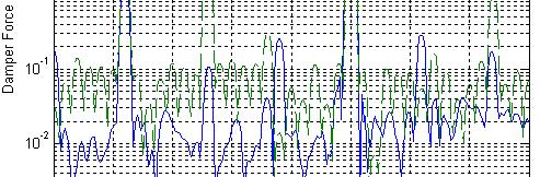
319 95 Figure F.4 A comparison of the experimental MR damper force steady state time histories between the DOF FFS prototype (-) and the model (---) using the simple MR damper model described in Table (F.) under the test conditions described in Table (F.3). Figure F.5 A comparison of the experimental MR damper force spectrum between the DOF FFS prototype (-) and the model (---) using the simple MR damper model described in Table (F.) under the test conditions described in Table (F.3).

320 96 A comparison of the experimental and model overall transmitted force time history and spectrum are shown in Figure (F.6) and (F.7). With a poor correlation between the spring and damper forces, the overall transmitted force is not expected to predict the experimental forces transmitted by the prototype. However, the spectrum shows the model predicts the force magnitude at the excitation frequency of 5 H. Of greater interest is the performance at the difference frequency, 6 H, and the model substantially over estimates the force magnitude. Figure F.6 A comparison of the experimental transmitted force steady state time histories between the DOF FFS prototype (-) and the model (---) using the simple MR damper model described in Table (F.) under the test conditions described in Table (F.3).

321 97 Figure F.7 A comparison of the experimental transmitted force spectrum between the DOF FFS prototype (-) and the model (---) using the simple MR damper model described in Table (F.) under the test conditions described in Table (F.3). Based on the spectrum force comparison, the simplified model typically over predicts the spring, damper, and transmitted force at the difference frequency and excitation frequency. The model under predicts the experimental result of the transmitted force produced by the prototype. The lack of correlation is the result of using simplified MR damper model that did not account for the complex variation dissipative properties due to a time varying control voltage. A comparison of the results of both the prototype and model are provided in Table (F.4). It was postulated that the damper force would not contribute significantly to the transmitted force and thus the modeling of the MR damper could be simplified. However, based on the comparison the time varying characteristics of the MR damper to a time varying control signal cannot be ignored for this application.

322 98 Table F.4 A summary of the comparison of the transmitted forces produced by the prototype and model. System Force Model Prototype [ N ] Excitation Frequency 5 H Spring Damper Transmitted Difference Frequency 6 H Spring Damper Transmitted F.3.4 Preliminary Performance Assessment Although the model was unable to capture the force frequency dynamics of the DOF prototype, a preliminary experimental performance assessment was conducted for a set of system parameters. The selected control signal setting for the MR damper is a sine wave with a peak-to-peak amplitude from 0.5 to 1.0 Volts with a frequency of 19 H. This is not expected to demonstrate the maximum transmitted capable of being produced with the DOF shaker. This process provides a single performance curve at the difference frequency for a single set of system parameters. The task of building a complete set of performance curves under various system settings with an accurate model to predict the response is proposed for future work. Table (F.5) provides a summary of the setting used during the performance assessment.

323 99 Table F.5 The system settings for the performance assessment of the DOF prototype during force frequency shifting operation. Excitation Frequency Range [H]: MR Damper Control Signal Wave Form: Sine Damping Frequency [H]: 19 Voltage Offset [V]: Voltage Amplitude [V]: 0.75 The rotating imbalance exciter supplied the excitation force to the prototype. The excitation frequency was manually adjusted from H in 0.5 H increments through the manipulation of the power supply voltage to the rotating imbalance exciter. With the damping frequency constant at 19 H, the difference frequency range of the assessment was H. At each excitation frequency, the steady state damper force and a fraction of the spring force were recorded and the total spring and transmitted force were calculated. Using the spectrum of the force time histories, the peak force at the difference frequency was determined. The frequency dependent force curves of the spring, damper and overall transmitted force are shown in Figure (F.8), (F.9), and (F.10).

324 300 Figure F.8 The transmitted spring force at the difference frequency of the DOF prototype ( ) with linear interpolation (---) under the conditions described in Table (F.5). The spring force generally increases with increasing difference frequency. The maximum spring force, almost 9 N, occurs around the first natural frequency of the system where the dynamic response is the greatest. A gradual increase in spring force occurs as the difference frequency approaches the natural frequency compared to a steeper decline seen after the natural frequency.

325 301 Figure F.9 The transmitted MR damper force at the difference frequency of the DOF prototype ( ) with linear interpolation (---) under the conditions described in Table (F.5). The overall trend in the damper force at the difference frequency, shown in Figure (F.9), is similar to that seen in the simulation studies. Excluding the results at 1 and 1.5 H, when examining the FFS shaker dynamics through simulation it was found that the damper force trends to ero as the difference frequency approaches the natural frequency. For the DOF prototype, decrease in the damper force occurs as the difference frequency approaches the natural frequency. The difference in behavior is likely a property of a two degree of freedom FFS shaker and/ or the difference in the properties of the MR damper compared to model used in the simulation. The damper force appears to increase after the passing the first natural frequency which was also observed in simulation. However, this trend is not conclusive since it is only supported with one experimental data point.

326 30 Figure F.10 The overall transmitted force at the difference frequency of the DOF prototype ( ) with linear interpolation (---) under the conditions described in Table (F.5). The overall trend of the transmitted force at the difference frequency, shown in Figure (F.10), is similar to the spring force. Comparing the transmitted force to the spring force, the destructive interference of the damper force is evident. The magnitude of the transmitted force is less than that of the spring force from H. Constructive interference occurs at 6 and 6.5 H. With the limited amount of data, it can only be assumed that the trend continues. Based on simulation studies the natural frequency is the transition point from destructive to constructive interference between the spring and damper forces. Based on the transmitted force, this trend also occurs experimentally.

327 303 F.4 Summary The design, development, and preliminary assessment of the DOF FFS prototype demonstrated significant transmitted force performance enhancement in a portion of the low frequency region. The additional system natural frequency placed on or near the excitation frequency appears to improve the transmitted force at the difference frequency. However, the assessment is incomplete and a full compliment of supporting evidence is needed to draw definitive conclusions. The system identification process carried out on the DOF prototype was performed with the intent on developing a numerical model of the system. The results of that process have shown the following: 1. The modeling developed through the acceleration free vibration response time history correlation was successful at determining the system properties of the DOF prototype.. The simple MR damper model based on static control voltage and corresponding dissipation parameters did not accurately represent the experimental DOF prototype dynamic behavior under a sinusoidal control voltage with known amplitude and offset. 3. The proposed solution for the continuation of this work is to revaluate the DOF system with the superior equipment and MR damper model used in the feedback control analysis of the SDOF system.

328 304 A preliminary performance assessment for a single MR damper control signal over a limited difference frequency range was performed. A complete assessment for a varied set of control signals with an improved frequency range is needed draw definitive conclusion about the performance gains that can be achieved using a DOF hardware design. The preliminary performance assessment has shown the following: 1. The DOF prototype experimental performance demonstrated trends observed in the dynamic analysis of the SDOF FFS translational system.. The settings selected for the performance evaluation are not characteristic of the maximum possible transmitted force gains achievable with the prototype. 3. The performance gains in the difference frequency range are expected to be the greatest on and around the first natural frequency of the prototype. 4. From the experimental results of the model comparisons maximum transmitted force gains can be expected be has high as 1% around the first natural frequency of the prototype.

329 305 APPENDIX G FFS Exciter System Identification in the DOF Configuration G.1 Introduction The nominal model parameters of the FFS prototype in the two degree of freedom configuration were determined through a systematic system identification process. The system identification process is carried out for the two individual subsystems providing a basis to judge the identification results in the DOF configuration. Experimental and analytical evaluation of the custom counter rotating imbalance exciter used to provide the high frequency excitation begins the identification analysis. The process continues with the determination of the equivalent mass, stiffness, and dissipative properties of the two individual subsystems and in the DOF configuration. G. Counter Rotating Imbalance Exciter Design The excitation of the FFS prototype in the DOF configuration was achieved with a counter rotating out of balance mass exciter, placed on the smaller top mass. A schematic is shown in Figure (G.1). A counter rotating design was necessary to limit the transmitted later forces that would prevent smooth vertical translation of the masses. If

330 306 properly aligned, the later forces produced by rotation of the individual masses should cancel resulting in only a sinusoidal vertical force. Figure G.1 Schematic of a counter rotating imbalance exciter. The rotating imbalance exciter uses a 4 Volt through axis DC motor mounted between two parallel aluminum plates to drive the eccentric mounted masses as shown in Figure (G.). Another shaft aligned with the motor shaft is mounted through the parallel plates adjacent to the motor. Identical gears are attached to the both shafts at each end. The gear mounted to the motor shaft meshes with the gear mounted to the adjacent shaft allowing counter rotation to cancel lateral forces. The gears are attached to the shafts via a setscrew for manual alignment.

331 307 Figure G. The rotating imbalance shaker used to excite the DOF FFS prototype. The imbalance masses are attached to 3 adjacent through holes of each gear. The out-of balance-masses simply consist of a screw and several nuts. Since all alignment is performed manually, the theoretical transmitted force could be difficult to achieve. Any misalignment will result in the creation of a transmitted moment, which is undesirable. G..1 Counter Rotating Imbalance Exciter Performance Force data was taken from the rotating imbalance shaker in order to characterie the transmitted force performance. The shaker was mounted to a plate, which in turn was mounted to four pieoelectric load cells as shown in Figure (G.3). The entire setup was anchored to an optical bench. The DC motor of the rotating imbalance shaker was connected to a power supply where the voltage was adjusted manually to achieve the desired rotational frequency.

332 308 Figure G.3 The experimental test setup for characteriing the transmitted force performance of the counter rotating imbalance exciter. The performance of the rotating imbalance shaker was characteried by calculating the transmitted force and moments at a typical operating frequency. The rotating imbalance shaker was set to operate at 5 H by manually adjusting the voltage of the power supply. The transmitted force was determined by summing the individual force signals from the 4 load cells using equation (G.1). ( t) F ( t) + F ( t) + F ( t) F ( t) F tr = G.1 The force transmitted at 5 H was 85 N, which was determined by calculating the spectrum of the transmitted force time history shown in Figure (G.4). The transmitted force time history also contains content at integer multiples of the operating frequency; however, there is a significant reduction of magnitude in the higher frequency content.

333 309 Figure G.4 The rotating imbalance shaker transmitted force time series and spectrum at 5 H. The shaker produces an 85 N force at 5 H and less significant forces at integer multiples of the test frequency. The layout of the four load cells used to record the transmitted force of the rotating imbalance exciter is shown in Figure (G.5). Load Cell 1 4 Plate Long Axis S=5.1 cm Plate Short Axis 3 L=17.7 cm Figure G.5 Schematic of the arrangement of the load cells used to record the forces during the evaluation of the rotating imbalance exciter.

334 310 Equation (G.) was used to determine the moment about the short plate axis. S S M LA = + G. ( t) [ F1 ( t) + F4 ( t) ] [ F ( t) F3 ( t) ] The moment about the long plat axis was calculated using equation (G.3). L L M SA = + G.3 ( t) [ F1 ( t) + F ( t) ] [ F3 ( t) F4 ( t) ] Figures (G.6) and (G.7) show the transmitted moment time history and corresponding spectrum about the long and short plate axis respectively. The moments produced by the rotating imbalance exciter, if significant, would limit the mobility of the smaller top mass of the prototype and degrade overall performance. The moment about the plate long axis is of a greater magnitude; however, it does not appear to be of sufficient magnitude to warrant an out of balance mass realignment. Figure G.6 The transmitted moment time history and spectrum about the plate long axis at 5 H.

335 311 Figure G.7 The transmitted moment time history and spectrum about plate short axis at 5 H. G.. Equivalent Out-of-Balance-Mass A correlation between the experimental and analytical equivalent out-of-balancemass of the rotating imbalance shaker was developed to determine the equivalent force to excite a DOF model and correlate with the experimental hardware. A poor correlation provides evidence of misalignment of the out-of-balance masses or an error in the modeling of the rotating imbalance shaker. The experimental equivalent out-of-balancemass was determined by fitting a quadratic trend line through transmitted force data at several frequencies and the analytical out-of-balance-mass was determined from the geometry and mass characteristics of the rotating imbalance design.

336 31 G...1 Analytical Equivalent Out-of-Balance Mass The equivalent out-of-balance-mass of the rotating imbalance shaker can be determined from the geometrical arrangement of the masses and the actual mass of the elements. For a single rotating imbalance mass the time varying transmitted force is found from equation (G.4). F ( t) m rω sin( ω t) = G.4 However, the rotating imbalance exciter has 3 imbalance masses, equidistant from the axis of rotation, on each gear as shown in Figure (G.8). Using the position of the second mass, m, as the reference, the time varying transmitted force for this arrangement is found from equation (G.5). ( t) = m rω sin( ωt + φ ) + m rω sin( ωt) + m rω ( ωt + φ ) F G sin 3 r φ 1 φ 3 m 3 m 1 m Figure G.8 The geometrical arrangement of the 3 out-of-balance masses on each gear of the rotating imbalance shaker.

337 313 Equation (G.5) is further expanded through the use of the trigonometric addition formula. Then, the magnitude of the equivalent force for one gear is determined from equation (G.6). 4 [ m cos( φ ) + m + m cos( φ )] + r ω [ m sin( φ ) m sin( φ )] 4 F EQ r ω = G.6 For this particular configuration, m 1 = m 3 = m o and φ 1 = 30 and φ 3 = -30 degrees. The resulting equivalent transmitted force magnitude is found from equation (G.7). ( m 3 + m ) ω FEQ = o r G.7 The out-of-balance-mass assemblies and the radial distance about which they rotate were measured. The mass m o and m were determined to be 1.7 grams and 11.8 grams respectively and the radial distance from the axis of rotation is approximately.54 cm. The analytical out-of-balance-mass for a single gear becomes kg m. Multiplying by four to account for the 4 gear subassemblies, the analytical out-ofbalance-mass for the rotating imbalance exciter is kg m. 3 3 G... Experimental Equivalent Out-of-Balance Mass The transmitted force produced by the rotating imbalance shaker was experimentally determined at 7 frequencies between 11 and 8 H. The transmitted force data was plotted as a function of frequency along with the best-fit quadratic curve as shown in Figure (G.9). The quadratic coefficient was determined to be kg m and

338 314 this is the experimentally determined out-of-balance-mass, which correlates extremely well with the analytical value of kg m. The experimental data shows a small increasing deviation from the model as the frequency increases resulting in a transmitted force greater than that predicted by the quadratic curve fit. Eccentric Mass Exciter Transmitted Force Frequency Response Experimental Quadratic Trend Force [ N ] Frequency [ rad/s ] Figure G.9 Experimental eccentric mass exciter transmitted force frequency response ( ) and best-fit quadratic curve (-). The out-of-balance-mass determined experimentally is in agreement with that determined analytically. The error is approximately 3%. With a correlation this strong, the out-of-balance masses were aligned extremely well. It was expected that the theoretical out-of-balance mass would be larger than the experimental. The smaller experimental transmitted force is accounted for in that a portion of the out-of-balancemass is wasted in the generation of a moment. The correlation suggests that manual alignment might be sufficient in the design of the rotating imbalance shaker.

339 315 G.3 Two Degree of Freedom System Identification A series of shake down tests were conducted on the subsystems that comprise the DOF FFS prototype. This was done to verify the system parameters used to describe the dynamics of the system. The selection of the springs and the design of the two masses were chosen to place the natural frequencies of the system. To improve low frequency excitation, the first natural frequency needed to be placed at the difference frequency and the second at the vertical excitation frequency. The anticipated excitation frequency was expected to be constant at 5 H and was selected as the second natural frequency. The first natural frequency was chosen to be 6 H such that increased excitation levels can be achieved on average between the 1 10 H frequency range. The prototype masses and springs were selected to achieve the desired natural frequencies. Free vibration tests of the prototype and the individual subassemblies were conducted. The systems were excited either with a given initial displacement or an impact. The acceleration response was recorded and an optimiation was performed to determine the system parameters based on minimiing the error between the experimental and model acceleration response. The system mass was weighed and therefore known, while the system stiffness was tightly constrained due to the information obtained from the spectrum of the free vibration response. The dissipation mechanism was assumed to be a combination of linear viscous and Coulomb friction damping. Under certain circumstances a forced vibration correlation was also developed. The peak acceleration response of the experimental system at the driving frequency was

340 316 compared to the model response under similar conditions. This was done over a range of excitation frequencies to provide another metric in assessing the identification of the system parameters of the prototype. G.3.1 Large Bottom Mass Subsystem Identification The DOF FFS prototype was disassembled to facilitate the vibration testing of the individual subsystems. The small top mass was separated from the large bottom mass by removing the two die springs coupling the two masses together. The four spring mounts supporting the large mass were left attached to the base and with the other components removed the linear rails and top structural plate were secured. The experimental setup to carry out the vibration testing of the larger bottom mass of the DOF FFS prototype is shown in Figure (G.10).

341 317 Figure G.10 The experimental setup to determine the large mass subsystem parameters. The large mass was placed into a state of free vibration with an initial displacement and the acceleration response was recorded. This was repeated three more times to obtain a total of four free vibration response of the large mass. A typical free vibration response is shown in Figure (G.11).

342 318 Figure G.11 Typical free vibration acceleration response of the large bottom mass subsystem component of the DOF FFS prototype The amplitude decay envelope is neither perfectly linear nor exponential, which would have indicated Coulomb friction or linear viscous damping. With no clear indication to a single dissipation mechanism, a model for this system was assumed to contain both linear viscous damping and Coulomb friction. The differential equation assumed to describe the free vibration response is presented in equation (G.8). & m& + c & + Ff + k = 0 G.8 & An optimiation routine using the fmincon function in MATLAB was developed to determine the system parameters. The routine allows for user defined constraints on parameters that can be adjusted to minimie a user defined objective function. The constrained adjustable parameters available to the optimiation routine included the initial conditions, the system stiffness, the linear viscous, and the Coulomb

343 319 friction damping. The mass was weighed and was therefore assumed to be a known quantity. The optimiation routine selected the parameters for the model represented by equation (G.8), which was numerically solved in Simulink. The optimiation routine perturbs the constrained parameters and calculates the resulting objective functions. The gradient is then calculated to determine the parameters and the adjustment direction that had the greatest influence in reducing the objective function. This process repeats until the objective function is minimied within a specified tolerance. The objective function of the optimiation was selected to express the sum of the squared error between the experimental and model acceleration response. The time location within the experimental data to begin the comparison was manually determined by examining the quality of the data and considering the model initial conditions required to match the experimental response. To accurately capture the experimental dynamics with the model determined through the optimiation, the error associated with the first three data points in the objective function was artificially weighted to ensure an accurate determination of the model initial conditions. Significant deviation between the initial behavior of the model produced by the optimiation routine and the experimental data resulted in an increase in the weight. The objective function, Q, to be minimied by the optimiation routine used to determine the system parameters is shown in equation (G.9). Minimie: 3 N Q = [ & exp ( n) && model ( n) ] D + [ && exp ( n) & model ( n) ] G.9 n= 1 n= 4

344 30 Constraints on the adjustable system parameters were developed to reduce the computational time needed by the iterative optimiation algorithm and ensure convergence to a solution. Constraints on the initial conditions were achieved by selecting a negative peak in the experimental acceleration response to begin the comparison with the model. Theoretically this implies the initial velocity is ero and the sign of the velocity is transitioning from negative to positive. The initial displacement is then limited to being a positive value. The constraint on the stiffness was developed through the spectrum of the free vibration response. The oscillation frequency was determined to be 7.38 H (46.3 rad/sec) from the spectrum of the free vibration response. From direct measurement, the mass was known to be 8.7 kg. If it is assumed that the free vibration frequency is approximately equal to the natural frequency, then the stiffness is equal to 1.87 x 10 4 N/m. However, this stiffness value differed significantly from that reported by the manufacturer. The stiffness of the individual springs supporting the large bottom mass was reported to be 3850 N/m. Four springs were used to support the large mass; the equivalent stiffness is 1.54 x 10 4 N/m. The resulting natural frequency was calculated to be 6.67 H (4.07 rad/ sec). With this small discrepancy, the actual stiffness value was believed to be located near the stiffness determined from the spectrum. A small interval centered around 1.87 x 10 4 N/m was used as the stiffness constraint. A list of the parameter constraints used in the optimiation is provided in Table (G.1).

345 31 Table G.1 The system parameter and initial condition constraints used in the optimiation routine to estimate the model parameters of the large bottom mass subassembly. Large Bottom Mass Optimiation Parameter Constraints System Parameters Stiffness [N/m]: k.0 10 Linear Viscous Damping [N s/m]: 0.1 c 5 Coulomb Friction Damping [N]: 0.1 F f Initial Conditions Initial Displacement [m]: Initial Velocity [m/s]: 0.01 & The optimiation routine was performed on the four experimental acceleration responses. The results from the optimiation routine produced estimates of the system stiffness, viscous and Coulomb friction damping. There is some uncertainty in the parameter estimates evident by the convergence of the optimiation to different parameter values for each response. The variation is most evident in the estimates of the dissipation parameters both the viscous and Coulomb friction damping. With no apparent mechanism of dissipation, this was expected. The average of the four estimates produced by the optimiation routine was assumed to be the actual parameter value. A summary of the optimiation results is presented in Table (G.). Table G. The system parameter estimates produced by the optimiation routine on the acceleration free vibration response of the larger bottom mass. Fixed System Optimiation Results Trial Parameter System Parameters Initial Conditions Mass K C F f X o V o [ kg ] [ N/m ] [ N s/m ] [ N ] [ m ] [ m/s ] x x x x Average x

346 3 Examining the correlation between the experimental and model acceleration responses can be sued to assess the accuracy of the results from the optimiation. The integration time step in calculating the model response was set to seconds to match the sample rate used to capture the experimental data. The simulation acceleration response with the parameters determined from the optimiation is compared to the experimental acceleration response in Figure (G.1). The optimiation accurately estimated the system stiffness due to the absence of a phase shift in the alignment of corresponding amplitude peaks. The match in corresponding amplitude height also provides evidence that the damping was estimated accurately. Figure G.1 Typical correlation results between the experimental acceleration response of the large bottom mass (-) and the model determined through the optimiation routine (---).

347 33 G.3. Small Top Mass Subsystem Identification The parameter identification process was repeated on the smaller top mass subsystem of the two-degree of freedom FFS prototype. The experimental setup, shown in Figure (G.13), was reconfigured to facilitate vibration testing of the smaller top mass. The linear bearings attached to the small top mass were placed on the linear rails and the two spring subassemblies were attached to the top face of the larger bottom mass. The larger bottom mass was used to anchor the top mass which required the removal of the four spring assemblies. Figure G.13 The experimental test setup used to initiate a free vibration response of the top mass subassembly to verify the system parameters.

348 34 Two die springs were used to connect the small top mass to the larger bottom mass. To initiate free vibration of the top mass required the use of an impact hammer due to the high stiffness of the die springs. The acceleration response was recorded for a total of four impact tests and a typical response is shown in Figure (G.14). Figure G.14 A typical acceleration free vibration response of the smaller top mass subassembly induced by an impact. The system model assumed for the larger mass, shown in equation (G.5), was also used to represent the dynamics of the smaller mass. The same optimiation routine was employed, with different constraints, to estimate the system parameters. The constraints on the system parameters are show in Table (G.3). The upper limits on both damping constraints were increased due to the reduced number of oscillations present in the free vibration response compared with the larger mass. The stiffness interval was again determined by analying the spectrum of the free vibration response.

349 35 Table G.3 The system parameter and initial condition constraints used in the optimiation routine to estimate the model parameters of the small top mass subassembly. Small Top Mass Optimiation Parameter Constraints System Parameters Stiffness [N/m]: k Linear Viscous Damping [N s/m]: 0.1 c 35 Coulomb Friction Damping [N]: 0.1 F f 3 Initial Conditions Initial Displacement [m]: Initial Velocity [m/s]: 0.01 & However, a small discrepancy in spring constants was observed. The reported stiffness value for the individual die springs was 3.5 x 10 4 N/m, which results in an equivalent system stiffness of 7.0 x 10 4 N/m. Using the known smaller mass,.1 kg, and the reported stiffness value of 7.0 x 10 4 N/m, the natural frequency can be approximated at 9.1 H (18.5 rad/sec) if the damping is small. The free vibration frequency of the top mass after impact was actually 31.5 H ( rad/sec). This results in a stiffness estimate of 8.1 x 10 4 N/m. The optimiation routine was performed using the four experimental acceleration responses and estimates of the system stiffness, viscous and Coulomb friction damping was produced. A summary of the optimiation results is presented in Table (G.4). The small statistical variation present in the parameter estimates resulted in assuming the average to be the actual parameter value.

350 36 Table G.4 The system parameter estimates produced by the optimiation routine on the acceleration free vibration response of the smaller top mass. Fixed System Optimiation Results Trial Parameter System Parameters Initial Conditions Mass K C F f X o V o [ kg ] [ N/m ] [ N s/m ] [ N ] [ m ] [ m/s ] x x x x Average 8.16 x A typical result comparing the acceleration response of the model produced by the optimiation and the actual experimental response are shown in Figure (G.15). An accurate representation of the system dynamics is achieved given the degree to which the two responses coincide. A significant amount of noise is present in the experimental response, but appears to have had little affect on the parameter estimation routine. Matching of amplitude height and the coincidence of amplitude peaks suggest an accurate estimate of the damping and stiffness. Figure G.15 Typical correlation results between the experimental acceleration response of the top mass (-) and the model determined through the optimiation routine (---).

351 37 G.3.3 Small Top Mass Forced Vibration Correlation A forced vibration test was conducted with the small mass to further assess the model developed through the optimiation routine. The counter rotating imbalance exciter was attached to the top of the small mass. The experimental setup to gather the steady state forced vibration acceleration response of the top mass is shown in Figure (G.16) and is similar to the previous setup to gather the free vibration acceleration data shown in Figure (G.13) with addition of the attached counter rotating imbalance exciter. Figure G.16 The experimental setup to obtain the steady state forced vibration acceleration response of the top mass.

352 38 The forced vibration acceleration response of the smaller top mass was captured with the rotating imbalance operating at 5 different frequencies between H. A sample time history of the acceleration response at steady state and corresponding spectrum is shown in Figure (G.17). The spectrum reveals the presence of one dominant acceleration frequency and several smaller harmonics. Figure G.17 The steady state acceleration response, time history and spectrum, of smaller top mass due to excitation from the rotating imbalance exciter at 18 H. From each acceleration response time history, the peak acceleration at the dominant excitation frequency was determined from the spectrum. The transient response was not included in the time history when the spectrum was calculated with a flattop window to preserve amplitude accuracy of the acceleration response. This analysis resulted in an experimental frequency dependent peak acceleration response. The experimental peak acceleration was compared to the analytical results developed from the system model. The system parameter estimates determined by the optimiation routine, along with the system mass, which was increased to account for the attached rotating imbalance shaker were used to produce the analytical acceleration

353 39 response. A frequency dependent excitation force based on the analysis of the rotating imbalance exciter was used as the input to the model. The peak acceleration response of the model was determined from 6 18 H. The steady state acceleration response at each frequency was determined and the spectrum calculated. The peak acceleration response at each frequency was extracted from the spectrum. A comparison of the peak acceleration frequency response determined experimentally and through simulation is shown in Figure (G.18). Figure G.18 The correlation between the experimental ( ) and model (-) steady state forced vibration peak acceleration response at several frequencies. The experimental peak acceleration response correlates with the model predictions. The model appears to accurately capture the peak acceleration at the driving frequency of rotating imbalance exciter of the smaller top mass. This provides more evidence that the parameter estimates produced by the optimiation routine were accurate.

354 330 G.3.4 System Identification in the DOF Configuration With estimates of the individual subsystem parameters shown to accurately capture the dynamics of the respective systems, vibration tests were conducted to validate the system parameters in the DOF configuration using techniques previously described. The free vibration acceleration response of both the smaller top and larger bottom masses were captured when the DOF system was subjected to an impact. Figure (G.19) typical free vibration responses of the smaller top mass and larger bottom mass. Evidence of the two natural frequencies is present in the response of each mass. Figure G.19 The acceleration free vibration response of the large bottom mass (-) and the smaller top mass (---) as a result of an impact in the DOF configuration. A two-degree of freedom model was developed to represent the dynamics of the prototype. The model is similar in from to the single degree of freedom models developed for the individual subassemblies. The dissipation assumed to remain uncoupled with no damping based on the relative motion between the two degrees of

355 331 freedom. The differential equation representing the model for the two-degree of freedom dynamics is shown in equation (G.10). New subscripts are introduced to identify the different degrees of freedom. The subscript L refers to the large bottom mass while the subscript S refers to the small top mass. m 0 L 0 && m S && L S cl & c S & L S F + F fl fs & & & & L L S S k L + k + ks S k k S S L S 0 = 0 G.10 The objective function, Q, used to aid the selection of the system parameters for the DOF prototype model shown in equation (G.11) and it is similar to the function utilied during the single degree of freedom optimiations. The objective function is defined by the sum of the weighed initial acceleration responses of both the top and bottom masses plus the squared error of the remaining acceleration responses of the top and bottom mass. The weight on the initial acceleration responses was manually selected to increase the initial correlation resulting in an accurate estimate of initial conditions. Minimie: Q = + 3 n= 1 3 n= 1 N [&& ( n) && ( n) ] D + && ( n) && ( n) L,exp [ L,exp L,model ] n= 4 N [&& ( n) && ( n) ] D + && ( n) && ( n) S,exp L,model S,model S L [ S,exp S,model ] n= 4 G.11 The system parameters estimates determined in the DOF configuration were not expected to deviate significantly from the SDOF parameter estimates. The damping optimiation constraint intervals for both the linear viscous and Coulomb friction damping were tightened. The stiffness constraints required adjustment as a result of the

356 33 change in configuration. With a more complicated system model and a total of 10 adjustable parameters, the tightening of constraints was desired to facilitate timely convergence to a set of parameter estimates. The spectrum of the free vibration response of the top and bottom masses was calculated to examine the frequency content. The natural frequencies of the system were determined to be 6.5 and H. To achieve these natural frequencies with system masses of 8.7 and.1 kg requires an equivalent stiffness of 16,780 and 85,650 N/m. These stiffness values differ from the results obtained from the equivalent stiffness estimated by the optimiation routine for the two subassemblies. The stiffness constraints contain the values that result from examining the free vibration frequency content. The initial condition optimiation constraints were also relaxed to account for the added degree of freedom. The relationship between acceleration, velocity, and displacement used to limit the SDOF initial condition optimiation constraints is not guaranteed to apply for a system with more than one degree of freedom. Greater latitude in the initial conditions was required resulting in larger constraint intervals. Although the free vibration acceleration response is initiated with an impact, the comparison between model and experimental free vibration response begins a cycle after impact requiring initial condition constraints on both the top and bottom masses. A list of the parameter constraints used in the DOF optimiation model is provided in Table (G.5).

357 333 Table G.5 The parameter optimiation constraints used in the routine to estimate the system parameters in the DOF configuration. DOF Optimiation Parameter Constraints Large Bottom Mass, m L System Parameters 4 4 Stiffness [N/m]: k L. 10 Linear Viscous Damping [N s/m]: 1.0 c L 3. 5 Coulomb Friction Damping [N]: 0.1 F fl 0. 9 Initial Conditions Initial Displacement [m]: 0.07 L Initial Velocity [m/s]: 0.1 & 0. 1 L Small Top Mass, m S System Parameters Stiffness [N/m]: k S c S Linear Viscous Damping [N s/m]: 35 Coulomb Friction Damping [N]: 1.0 F fs. 5 Initial Conditions Initial Displacement [m]: 0.07 S Initial Velocity [m/s]: 0.1 & 0. 1 S 10 4 The optimiation routine determined initial conditions and the system parameters for both degrees of freedom that minimied the objective function utiliing the experimental and model acceleration response. The results from the optimiation routine on the four separate impact induced free vibration responses of the DOF prototype are presented in Table (G.6) and (G.7). The linear viscous and Coulomb friction damping estimates are similar to the SDOF optimiation estimates. An unexpected change in stiffness, revealed earlier in the free vibration spectrum, resulted from a change in the configuration.

358 334 Table G.6 Optimiation results for the estimation of the larger bottom mass parameters based on an impact induced free vibration acceleration response in the DOF configuration. Fixed System Optimiation Results Parameter System Parameters Initial Conditions Trial Mass K L C L F fl X o V o [ kg ] [ N/m ] [ N s/m ] [ N ] [ m ] [ m/s ] x x x x Average 1.85 x Table G.7 Optimiation results for the estimation of the small top mass parameters based on an impact induced free vibration acceleration response in the DOF configuration. Fixed System Optimiation Results Parameter System Parameters Initial Conditions Trial Mass K S C S F fs X o V o [ kg ] [ N/m ] [ N s/m ] [ N ] [ m ] [ m/s ] x x x x Average 8.58 x The optimiation produced results that accurately reflect the system dynamics, which are evident through graphical comparison. The integration time step in calculating the model response was set to seconds to match the sample rate used to capture the experimental data. A typical correlation result comparing the result from the model based on parameters from the optimiation and the experimental acceleration response is shown in Figures (G.0) and (G.1). The optimiation predicted an increase in stiffness associated with the larger bottom mass and the smaller top mass. However, there was no significant change apparent in the damping. The average value was assumed to be the estimate of the parameter.

359 335 Figure G.0 Typical correlation results between the experimental acceleration response of the large bottom mass (-) and the model (---) determined through the optimiation routine in the DOF configuration. Figure G.1 Typical correlation results between the experimental acceleration response of the small top mass (-) and the model (---) determined through the optimiation routine in the DOF configuration.

360 336 G Forced Vibration Acceleration Correlation The rotating imbalance exciter was attached to the smaller top mass to develop a correlation of the peak steady state acceleration between the model and the experimental response of the DOF prototype. The excitation frequency range was from 10 0 H and the acceleration responses of both the top and bottom masses were recorded at each frequency. The spectrum of the steady-state acceleration response was calculated to determine the peak acceleration at the driving frequency of the shaker. The model was then used to produce the analytical acceleration response due to excitation by the rotating imbalance. Parameters from the optimiation were used and the smaller top mass was increased to account for the mass of the rotating imbalance exciter. The frequency dependent force produced by the rotating imbalance exciter was applied to the smaller top mass in the model. The peak steady state acceleration response produced by the model was determined over a wide frequency range. These results were then compared with the experimental acceleration response. The comparison is shown in Figure (G.).

361 337 Figure G. Steady state peak acceleration correlation between the bottom large mass experimental ( ) and the model (-) response along with the small top mass experimental ( ) and model response (---) in the DOF configuration. The model accurately captures the dynamic behavior of the DOF prototype. The model under predicts the acceleration of the large top mass for frequencies greater than 14 H. The discrepancy between the acceleration response and the model for the larger top mass is small with maximum error of 10.5% occurring at 13.9 H. A strong correlation in the acceleration response also exists between the model and the smaller top mass. The model captures the anti-resonance behavior in the smaller mass apparent at approximately 17.5 H. The correlation supports the accuracy of the parameter estimates obtained by the optimiation routine.

362 338 G.3.4. System Identification with the MR Damper The MR damper was added to the DOF prototype assembly. The damper connects to a bracket located on the bottom face of the smaller top mass and the cylindrical fixture located in the center of the base plate. The experimental setup to capture the free vibration data is shown in Figure (G.3). Vibration tests were again carried out to determine the system parameters with the MR damper included in the assembly. During the tests, a control voltage was not applied to the MR damper amplifier. a b Figure G.3 Experimental setup, picture (a) and SolidWorks model (b), used to capture the acceleration response of the top and bottom mass with the MR damper added to the assembly.

363 339 Adjustments to the system parameters and the optimiation constraints were needed due to the addition of the MR damper to the assembly. An increase of 0.5 kg to the top mass was needed to account for the attached MR damper. From the analysis developed in [9], under static control input conditions, the MR damper can be modeled as a linear viscous and Coulomb friction damper acting in parallel. Therefore, the damping constraints associated with the smaller top mass were increased to account for the expected increase in dissipation due to the addition of the MR damper. The adjustments to the constraints are listed in Table (G.8). The remaining constraints and the objective function can be reviewed in Table (G.5) and equation (G.9) respectively. Table G.8 The new constraints made to the small top mass damping parameters to account for the addition of the MR damper to the assembly. Small Top Mass, m S System Parameters Linear Viscous Damping [N s/m]: 0 c S 40 Coulomb Friction Damping [N]: F 5 fs The system was excited with an impact hammer and the acceleration responses were again recorded. The optimiation routine, using the error between the experimental and numerical model produced parameter estimates that minimied the objective function. The parameter estimates developed by the optimiation routine are presented in Table (G.9) and (G.10).

364 340 Table G.9 Optimiation results for the estimation of the large bottom mass with the addition of the MR damper to the assembly. Fixed System Optimiation Results Trial Parameter System Parameters Initial Conditions Mass K L C L F fl X o V o [ kg ] [ N/m ] [ N s/m ] [ N ] [ m ] [ m/s ] x x x x Average 1.73 x Table G.10 Optimiation results for the estimation of the small top mass with the addition of the MR damper to the assembly. Fixed System Optimiation Results Trial Parameter System Parameters Initial Conditions Mass K S C S F fs X o V o [ kg ] [ N/m ] [ N s/m ] [ N ] [ m ] [ m/s ] x x x x Average 8.53 x The change in the dynamics due the addition of the MR damper resulted in a change of the system parameter estimates. The damping and stiffness terms associated with the large bottom mass did not see a statistically significant change. A significant change is present in the small top mass damping terms as a result of the MR damper. Comparing to the parameter estimates obtained without the MR damper, it can be assumed that the MR damper increased the linear viscous damping by 4.9 N s/m and the Coulomb friction damping by 1.5 N. The model developed from the optimiation and the experimental acceleration responses are graphically compared to assess the parameter estimation. A typical result of the correlation obtained between the acceleration responses of the large bottom mass is

365 341 shown in Figure (G.4). The peak amplitudes of the experimental free response and the model occur at the approximately the same time suggesting that the model has accurately estimated the stiffness of the system. The consistently smaller amplitude of the model provides evidence that the model has overestimated the damping. Figure G.4 Typical optimiation correlation results of the large bottom mass experimental (-) and model (---) free vibration acceleration response in the DOF configuration with the MR damper. Examining the spectrum of the free vibration acceleration responses, shown in Figure (G.5), provides more evidence supporting the ability of the model to accurately capture the system behavior. The spectrum peaks of both the experimental and the model free vibration acceleration response occur at 7.5 and 35 H. As noted with the time series correlation, this provides further confidence on the system stiffness estimates. However, the magnitude is greater in the experimental response with the larger discrepancy occurring at the 35 H natural frequency suggesting that the damping parameters have been overestimated.

366 34 Figure G.5 Typical optimiation correlation results of the large bottom mass experimental (-) and model (---) acceleration spectrum of the free vibration response due to an impact in the DOF configuration with the MR damper. The correlation between the free vibration acceleration time histories of the small top mass is shown in Figure (G.6). As seen with the correlation with the large bottom mass, the model of the response of the small top mass accurately captures the system stiffness evident through the lack of phasing between the peak amplitude of the experimental and model acceleration response. The overall model amplitude is consistently of a smaller magnitude than the experimental response. Again, this is similar to the correlation seen with the large bottom mass.

367 343 Figure G.6 Typical optimiation correlation results of the small top mass experimental (-) and model (---) free vibration acceleration response in the DOF configuration with the MR damper. The spectrum of the free vibration acceleration experimental and model response revealed the presence of the 7.5 and 35 H natural frequencies. Evident through the spectrum in Figure (G.7), there is only a minor amplitude discrepancy with the experimental peak at 7.5 and 35 H being slightly larger in magnitude than the model. Overall, the parameter estimates for the smaller top mass appear more accurate. There appears to be a discrepancy in the location of the system anti-resonance between the experimental response and the model at 14 H and this is not easily detected in the time series correlation.