Pipeline Inspection Technologies Demonstration Report Final

Transcription

1 University of Nebraska - Lincoln DigitalCommons@University of Nebraska - Lincoln United States Department of Transportation -- Publications & Papers U.S. Department of Transportation 26 Pipeline Inspection Technologies Demonstration Report Final Follow this and additional works at: Part of the Civil and Environmental Engineering Commons "Pipeline Inspection Technologies Demonstration Report Final" (26). United States Department of Transportation -- Publications & Papers This Article is brought to you for free and open access by the U.S. Department of Transportation at DigitalCommons@University of Nebraska - Lincoln. It has been accepted for inclusion in United States Department of Transportation -- Publications & Papers by an authorized administrator of DigitalCommons@University of Nebraska - Lincoln.

2 Pipeline & Hazardous Materials Safety Administration Pipeline Inspection Technologies Demonstration Report Pipeline Safety Research & Development Program Final

3 EXECUTIVE SUMMARY The pipeline infrastructure is a critical element in the energy delivery system across the United States. Its failure can affect both public health and safety directly and indirectly through impacts on the energy supply. The pipeline infrastructure is aging, while at the same time Research & Development (R&D) funding from the pipeline industry to develop technologies to assure its integrity is experiencing budgetary constraints. Total R&D funding is being further reduced through the elimination of programs resulting from restructuring within the government and energy industry. The Pipeline & Hazardous Materials Safety Administration (PHMSA), Pipeline Safety R&D Program mission is to ensure the safe, reliable & environmentally sound operation of the nation s pipeline transportation system. With passage of the Pipeline Safety Improvement Act (PSIA) in 22, industry is now required to invest significantly more capital to inspect and maintain their systems. The PSIA requires enhanced maintenance programs and continuing integrity inspection of all pipelines located within high consequence areas where a pipeline failure could threaten public safety, property and the environment. According to the Interstate Natural Gas Association of America (INGAA) the cost to industry to implement the PSIA in the first ten years will exceed $2 billion. The focus of the PHMSA Pipeline Safety R&D Program is to sponsor research and development projects intended on providing near-term solutions that will improve the safety, reduce environmental impact, and enhance the reliability of the nation s pipeline transportation system. Conducting infield technology demonstration test to facilitate technology transfer from government funded R&D programs strengthens communication and coordination with industry stakeholders The keys to enhanced pipeline safety are understanding the risks, focusing on the problems, imagining solutions, and applying our ingenuity Ted Willke. The PHMSA Pipeline Safety R&D Program role in technology development and innovation has increased with the passage of the Pipeline Safety Improvement Act of The implementation of the Integrity Management Program for natural gas and hazardous liquids has focused efforts on proactively finding and fixing safety-related problems. For several years the PHMSA Pipeline Safety R&D Program along with the DOE/NETL, Gas Delivery Reliability Program have funded the development of advanced in-line inspection (ILI) technologies to detect mechanical damage, corrosion and other threats to pipeline integrity. Several projects have matured to a stage where demonstrations of their detection capability are now warranted. During the week of January 9 th, 26, the PHMSA Pipeline Safety R&D Program and the DOE/NETL, Gas Delivery Reliability Program co-sponsored a demonstration of six innovative technologies

4 The demonstrations were conducted at Battelle West Jefferson s Pipeline Simulation Facility (PSF) near Columbus, Ohio. The pipes used in the demonstration were prepared by Battelle at the PSF and each was pre-calibrated to establish baseline defect measurements. Each technology performed a series of pipeline inspection runs to determine their capability to detect and size mechanical damage, corrosion, stress corrosion cracking or plastic pipe defects. Overall, each technology performed well in their assessment category. BACKGROUND Information regarding inspection technology advances needs to be disseminated and understood by many stakeholders in the pipeline industry. While research reports, review meetings and conference presentations are commonly used to disseminate information, live demonstrations can provide additional information on the current state and future potential of each development. Demonstrations are challenging to technology developers because newly developed technologies must be sufficiently reliable to obtain results in a fixed time frame. There is not the opportunity to return to the laboratory to confirm results or change parameters. While the pressure to demonstrate the best capability of their technology advances is enormous, the developers understand these events are needed to bolster support for continued development. The results of demonstrations can be difficult to directly compare since each implementation can be at a different stage of development. No direct comparisons were made in this report. At this demonstration, representatives from the pipeline industry, industry trade associations, and pipeline service providers were able to witness the performance of six new technologies and interact with technology developers to clarify the current and potential capability of these new developments. The participation of these groups was an essential element of the demonstration. This is the second benchmark of emerging pipeline inspection technologies performed by Battelle for DOT PHMSA Pipeline Safety R&D Program and DOE NETL. Information on the pipe defect sets, pipe preparation, demonstration facility layout, and demonstration procedures from the first test can be can be found in the final report, Benchmarking Emerging Pipeline Inspection Technologies 2, prepared by Battelle. The results from the first benchmarking can be found in the Pipeline Inspection Technologies - Demonstration Report 3, prepared by NETL. Purpose This report provides a brief summary assessment of the demonstration benchmark results. The purpose of this assessment is to help identify promising inspection technologies best suited for further development as part of an integrated teaming effort between robotic platform and sensor developers. This report is not intended to provide a detailed analysis of each technology s performance or to rate their performance relative to one another

5 The Technologies Six innovative sensor technologies were demonstrated at Battelle s Pipeline Simulation Facility (PSF) the week of January 9, 26. The different technologies demonstrated their ability to detect pipeline corrosion, mechanical defects, stress corrosion cracking, or plastic pipe defects. Additional information on each technology may be found in both Appendix B and Appendix C. The technologies were: ORNL Shear Horizontal Electromagnetic Acoustic Transducer (EMAT) Oak Ridge National Laboratory (ORNL) has developed an EMAT system that uses shear horizontal waves to detect flaws on natural gas pipelines. A wavelet-based analysis of ultrasonic sensor signals is used for detecting physical flaws (e.g., SCC, circumferential and axial flaws, and corrosion) in the walls of gas pipelines. Using an in-line non-contact EMAT transmitter-receiver pair, flaws can be detected on the walls of the pipe that the current magnetic flux leakage (MFL) technology has problems detecting. One EMAT is used as a transmitter, exciting an ultrasonic impulse into the pipe wall while the second EMAT located a few inches away from the first is used as a receiving transducer. ORNL s technology is depicted in Figure 1. Figure 1. ORNL Shear Horizontal EMAT GTI Remote Field Eddy Current (RFEC) The Gas Technology Institute (GTI) has developed a RFEC inspection technique to inspect pipelines with multiple diameters, valve and bore restrictions, and tight or miter bends. This electromagnetic technique uses a simple exciter coil that can be less than on third of the pipe diameter and is driven by a low-frequency sinusoidal current to generate an oscillating electromagnetic field that small sensor coils can detect. The oscillating field propagates along two paths; a direct axial path and an indirect or remote path. 4

6 The direct field attenuates rapidly because the pipe acts as a waveguide that will only allow frequencies in the gigahertz range and above to propagate. It becomes negligible after 2 to 3 pipe diameters. Thus after 2 to 3 pipe diameters, the only signal left is that from the remote field, which propagates out through the pipe wall, along its exterior and then re-enters the pipe 2 to 3 pipe diameters from the exciter coil. This is exactly what is needed for defect detection since the electromagnetic waves must now pass directly through metal loss defect regions and other flaws. Changes from nominal values of the amplitude and phase of the remote field detect defects in the pipe wall and measure their severity. GTI s technology is depicted in Figure 2. MUX Board Mock Explorer Module Support Sensor Coils Figure 2. GTI Remote Field Eddy Current Drive Coil SwRI Remote Field Eddy Current (RFEC) Through funding support from PHMSA/OPS, Southwest Research Institute has developed a remote-field eddy current (RFEC) technology to be used in unpiggable lines. The SwRI RFEC tool is capable of detecting corrosion on the inside or outside pipe surface. Since a large percentage of pipelines cannot be inspected using smart pig techniques because of diameter restrictions, pipe bends, and valves, a concept for a collapsible excitation coil was developed but found unnecessary for the pipe sizes and materials of interest in this demonstration. A breadboard system that meets the size, power, and communication requirements for integration into the Carnegie Mellon Explorer II robot was developed and used in the demonstration tests. This system is shown in Figure 3. The demonstration system incorporates eight detectors, and data from all eight channels are acquired and processed simultaneously as the system is scanned along the pipe at speeds up to 4 inch/sec. All of the instrumentation, except for a DC power supply and a laptop computer (used for storage of the processed data), is located on the tool. The RFEC system can expand to inspect 6- or 8-inch-diameter pipe and can retract to 4 inches to pass through obstructions. 5

7 Laptop Computer with CAN Bus Interface Electronics Encoder Wheel Sensors Excitation Coil DC Power Supply Figure 3. SwRI Remote Field Eddy Current PNNL Ultrasonic Strain Measurement Pacific Northwest National Laboratory (PNNL) has developed an ultrasonic sensor system capable of detecting pipeline stress and strain caused by mechanical damage i.e., dents and gouges. PNNL has established the relationship between residual strain and the change in ultrasonic response (shear wave birefringence) under a uniaxial load. Initial measurements on samples in both axial and biaxial states have shown excellent correlation between shear birefringence measurements. The demonstration focused on refining the methodology, particularly under circumstances when the damage is more complex than a simple uniaxial deformation. PNNL s technology is depicted in Figure 4. 6

8 EMAT Sensor Springs for smooth motion past dents Motor for sensor rotation Figure 4. PNNL Ultrasonic Strain Measurement Rotating Permanent Magnet Battelle is developing a rotating permanent magnet inspection system where pairs of permanent magnets are rotated around the central axis. This alternative to the more common concentric coil method can be used to induce high current densities in the pipe. Along the pipe away from the magnets in either direction, the currents flow in the circumferential direction. Anomalies and wall thickness variations are detected with an array of sensors that measure local changes in the magnetic field produced by the current flowing in the pipe. The inspection methodology can be configured to pass tight restrictions and narrow openings such as plug valves. The separation between the magnets and the pipe wall is on the order of an inch (2.5cm). The strength of circumferential current produces signals on the order of a few gauss, which can be detected by hall effect sensors positioned between 8 and 4 inches (1 and 1 cm) away from the rotating magnets. This evolving inspection methodology was first demonstrated in summer of 24. Battelle s technology is depicted in Figure 5. 7

9 Figure 5. Battelle Rotating Permanent Magnet Capacitive Sensor for Polyethylene Pipe Inspection The National Energy Technology Laboratory (NETL) has developed a capacitive probe to resolve defects in plastic natural gas pipelines. This new technology uses a non-destructive and non-hazardous projected electric field to map voids and other anomalies. The probe can function autonomously and is intended for use in conjunction with existing pigs or on its own platform. NETL s technology is depicted in Figure 6. Figure 6. NETL Capacitive Sensor 8

10 Demonstration Configuration The emerging inspection technologies were tested within a 4 by 1 foot high-bay area at Battelle s PSF. Pipes selected for these tests had various types of natural and machined defects. A black tarp and bubble wrap covered the pipes to hide defect locations. Figure 7 shows the configuration of the pipes during the demonstration. These pipes included: Figure 7. High-bay Looking North Detection of Metal Loss One 8-inch diameter ERW seam welded pipe measuring 3-feet in length (.188 inch wall thickness). The pipe sample contained two rows of simulated corrosion defects spaced 18 apart. One 8-inch diameter ERW seam welded pipe measuring 35-feet in length (.188 inch wall thickness). The pipe sample contained two rows of simulated corrosion defects spaced 18 apart. This sample also included a 5-foot section of natural corrosion from a pipe pulled from service. One 8-inch diameter ERW seam welded pipe measuring 4-feet in length (.188 inch wall thickness). The pipe sample contained two rows of simulated corrosion defects spaced 18 apart. 9

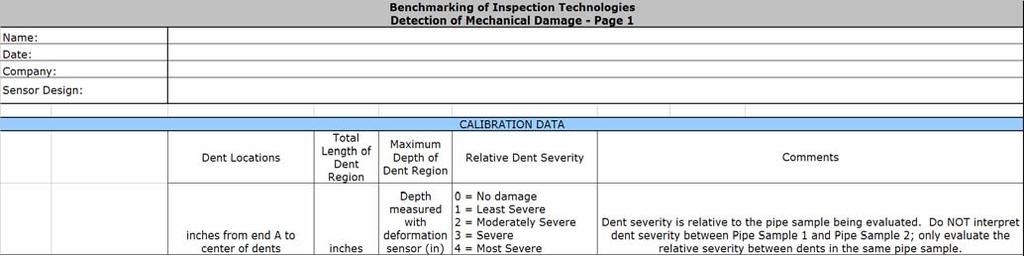
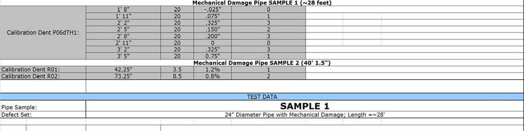
11 Detection of Mechanical Damage One 24-inch diameter pipe measuring approximately 28-feet in length (.292 inch wall thickness) comprised of two separate pipes welded together with mechanical damage defects. Three rows of mechanical damage defects were located on this pipe sample spaced 12 apart but only one row with track hoe defects were used in the benchmarking. One 24-inch diameter pipe measuring approximately 4 feet in length (.292 inch wall thickness) with plain (or smooth) dent defects along one row. Detection of Stress Corrosion Cracking (SCC) One 26-inch diameter pipe measuring approximately 26 feet in length (.281 inch wall thickness) with natural stress corrosion cracking. A separate 26-inch diameter SCC pipe sample was provided for calibration. Detection of Plastic Pipe Defects One 6-inch diameter polyethylene pipe measuring 13 feet in length (.5 inch wall thickness) with cylindrical drill holes and saw cut defects along one row on the exterior of the pipe. Additional information on the pipe defect sets, pipe preparation, demonstration facility layout, and demonstration procedures can be found in the final benchmarking report, Pipe and Anomaly Configuration for the Phase II Benchmarking of Emerging Pipeline Inspection Technologies prepared by Battelle and included in Appendix D. DEMONSTRATION RESULTS This section provides an assessment of the test data relative to the benchmark data developed at the Battelle Pipeline Simulation Facility (PSF). The benchmark data is provided as Appendix A of this document and test results for the individual technologies, as prepared and submitted by the technology developers, can be found in Appendix B. Metal Loss Corrosion Assessment The three corrosion assessment technologies were demonstrated in an 8-inch diameter pipe 4. This diameter was chosen to match a specific crawler implementation, Explorer, being separately developed under NETL DOE and Northeast Gas Association (NGA) funding 5. The untethered platform is designed to traverse pipelines ranging from 6 to 8 inches inside diameter. The inspection technology developers were asked to include as many of the configuration and interface requirements of this platform as practical. Three 8-inch diameter pipes were inspected by each technology for corrosion. The first pipe (Pipe Sample 1) was a seam-welded pipe measuring approximately 35 feet in length. This sample consisted of three pipe sections welded together (two circumferential welds) and 4 In the first demonstration these technologies were demonstrated in 12-inch diameter pipe

12 contained simulated corrosion defects set along two test lines 18 apart. The simulated corrosion was created using electrochemical etching techniques, an example of which is shown in Figure 8. A 5 foot section of Pipe Sample 1 also contained natural corrosion from a pipe recently pulled from service. Figure 8. Example Simulated Corrosion Defect using Electrochemical Etching Techniques The donated natural corrosion pipe sample had a field girth weld with corrosion on both sides of the weld. The weld drop through was too large for the inspection tool specifications and as such the pipe was trimmed to include roughly 2 feet of corrosion on one end, 3 feet of full thickness pipe at the other end, and no field welds. The pipe was then sandblasted and welded between two new pipes to comprise Pipe Sample 1. When the pipe was being fully characterized, an additional weld was found in the middle of the corrosion area (see Figure 9). This weld was very fine and did not have a significant crown. The natural corrosion defects were intended to be a stretch goal of these emerging inspection technologies. While the natural corrosion sample represents a real world problem, this additional weld adds a complex scenario that is most likely new to the technology developers. As such, these search areas are reported but are not included in the results evaluation. 11

13 Field Weld Figure 9. Fine, Field Weld in Natural Corrosion Pipe Segment The second pipe (Pipe Sample 2) was a seam-welded pipe measuring approximately 3 feet in length. This sample consisted of two pipe sections welded together (one circumferential weld) and contained simulated corrosion defects set along two test lines 18 apart. The third pipe (Pipe Sample 3) was a seam-welded pipe measuring approximately 4 feet in length. This sample consisted of two pipe sections welded together (one circumferential weld) and contained simulated corrosion defects along two test lines 18 apart. All three technologies detected one false positive signal; however, none of the technologies had a false positive in the same location. None of the technologies failed to identify a defect and were fairly accurate in predicting the locations. These results are summarized in Table 1. In addition, the corrosion sizing results were plotted in a manner commonly used by pipeline inspection vendors to demonstrate commercial in-line inspection technology capabilities. For these graphs, benchmark data is plotted against the values reported by the technology developers. Care must be taken in interpreting these graphs since: Error in the benchmark measurements is not zero Only the maximum depth is compared while the corrosion pit depth varied throughout the defect; many corrosion areas had more than one area of local thinning. Length and width were measured at the surface; however other measures can also be used that still accurately describe the anomaly. Overall these graphs show the results predicted by each technology correlated well with the benchmark data. 12

14 Table 1. Detection Rates for the Corrosion Technologies Technology Detection Rate SwRI RFEC 1% (32 of 32) GTI RFEC 1% (32 of 32) Battelle Rotating Permanent Magnet 1% (32 of 32) False Positive Rate 3.3% (1 of 3) Defect P2-8 called as a repeatable signal, but does not have typical flaw signal characteristics;.17 deep, 1.38 long and 1.6 wide 3.3% (1 of 3) Defect P1-2 called as an unknown feature resembling metal loss;.8 deep, <1 long, and >4 wide 3.3% (1 of 3) Defect P1-17 called as a small single pit.2 deep,.7 long, and.75 wide False Negative Rate % ( of 32) % ( of 32) % ( of 32) Mean Difference in Location of Defect Standard Deviation of Defect Location SwRI Results SwRI began testing the morning of Monday, January 9, 26, and completed testing by mid-day Thursday, January 12, 26. The SwRI RFEC tool acquired, processed, and displayed data in real time as it was continuously pulled through each pipe sample. Each scan took approximately 5 minutes to complete with selected higher speed runs taking approximately one to two minutes to complete. A circumferential region of 6 degrees was inspected in each scan, and two scans were made along each defect line to ensure complete coverage of all defects. The SwRI RFEC technology detection rate was 1%, detecting all defect sites on Pipe Sample 1, Pipe Sample 2, and Pipe Sample 3. On average, SwRI located anomalies slightly past the actual start of the defect location with a standard deviation of 1.71 inches. The SwRI RFEC technology detected one false positive signal on Test Line 1 of Pipe Sample 2. The false positive signal was identified as a repeatable signal without typical flaw signal characteristics with a depth of nearly 9% of the wall thickness and approximately 1 5/8 -inch in length. SwRI s sizing accuracy is depicted in Figures 1 through 12 in which the predicted and measured anomaly depths, lengths, and widths are presented. 13

15 Predicted Depth (inches) Measured Depth (inches) Figure 1. Measured Depth vs. Predicted Depth for the SwRI RFEC Predicted Length (inches) Measured Length (inches) Figure 11. Measured Length vs. Predicted Length for the SwRI RFEC 14

16 3 2.5 Predicted Width (inches) Measured Width (inches) Figure 12. Measured Width vs. Predicted Width for the SwRI RFEC GTI Results GTI began testing on the morning of Monday January 9, 26 and completed testing by the evening of Thursday January 12, 26. The GTI RFEC sensor technology collected data by indexing through each defect region in.25 inch steps. The GTI RFEC technology was able to scan both test lines in each pipe sample at the same time but because of the small incremental data collection each pipe sample required a full day to collect data. GTI did attempt a continuous scan with the results of this scan provided in Appendix C. The GTI RFEC technology detection rate was 1%, detecting all defect sites on Pipe Sample 1, Pipe Sample 2, and Pipe Sample 3. On average, GTI located anomalies slightly past the actual start of the defect location with a standard deviation of 1.18 inches. The GTI RFEC technology detected one false positive signal on Test Line 1 of Pipe Sample 1 but identified the anomaly as a small unknown feature with a depth of only 4% of the wall thickness and approximately 1-inch in length. GTI s sizing accuracy is depicted in Figures 13 through 15 in which the predicted and measured anomaly depths, lengths, and widths are presented. 15

17 Predicted Depth (inches).188 Measured Depth (inches) Figure 13. Measured Depth vs. Predicted Depth for the GTI RFEC Predicted Length (inches) Measured Length (inches) Figure 14. Measured Length vs. Predicted Length for the GTI RFEC 16

18 Predicted Width (inches) Measured Width (inches) Figure 15. Measured Width vs. Predicted Width for the GTI RFEC Battelle Results Battelle began testing the afternoon of Tuesday January 1, 26 and completed testing by the afternoon of Friday January 13, 26. Battelle s testing was periodically interrupted due to concerns from the other corrosion inspection technology developers that the permanent magnet was causing interference with their systems. The Battelle Rotating Permanent Magnet technology was able to continuously acquire data through each pipe sample taking approximately 1 to 15 minutes to scan one test line. During the demonstration Battelle processed signals and displayed inspection results in real-time. The Battelle Rotating Permanent Magnet technology detection rate was 1%, detecting all defect sites on Pipe Sample 1, Pipe Sample 2, and Pipe Sample 3. On average, Battelle located anomalies shy of the actual start of the defect location with a standard deviation of 2.5 inches. The Battelle Rotating Permanent Magnet technology detected one false positive signal on Test Line 2 of Pipe Sample 1 but identified the anomaly as a small single pit with a depth of only 11% of the wall thickness and approximately 3/4-inch in length. Battelle s sizing accuracy is depicted in Figures 16 through 18 in which the predicted and measured anomaly depths, lengths, and widths are presented. 17

19 Predicted Depth (inches) Measured Depth (inches) Figure 16. Measured Depth vs. Predicted Depth for the Battelle Rotating Permanent Magnet Predicted Length (inches) Measured Length (inches) Figure 17. Measured Length vs. Predicted Length for the Battelle Rotating Permanent Magnet 18

20 3 2.5 Predicted Width (inches) Measured Width (inches) Figure 18. Measured Width vs. Predicted Width for the Battelle Rotating Permanent Magnet The benchmark data and test results for the three technologies that tested for metal loss on Pipe Samples 1, 2, and 3 are shown in Table 2 through Table 7. 19

21 This page intentionally blank. 2

22 Table 2. Benchmark Data vs. Results for Corrosion Pipe Sample 1; Test Line 1 Simulated Corrosion Pipe Sample 1 Test Line 1 Defect Number P1-1 P1-2 P1-3 P1-4 P1-5 P1-6 P1-7 P1-8 P1-9 P1-1 P1-11 P1-12 Search Region (from End B) 328" to 34" 34" to 316" 28" to 292" 256" to 268" 232" to 244" 28" to 22" 184" to 196" 16" to 172" 12" to 144" 1" to 112" 76" to 88" 52" to 64" Start and End of Defect (inches) Blank Benchmark Data Blank Blank " Blank Blank Blank " a=12. SwRI RFEC b= GTI RFEC ~ ~ ~26.5 ~232 ~ ~12 ~56.75 ~ ~285.5 ~ ~236.5 ~ ~ ~6.5 Battelle Rotating Permanent Magnet Defect Length (inches) Benchmark Data Blank Blank Blank Blank 2.25 Blank Blank SwRI RFEC a=2.25 b= GTI RFEC < Battelle Rotating Permanent Magnet Defect Width (inches) Benchmark Data Blank Blank Blank 2 Blank Full Circ. Blank Blank 2 SwRI RFEC Full Circ. a=1.82 b=full Circ GTI RFEC > ~3 > > Battelle Rotating Permanent Magnet Maximum Defect Depth (inches) Benchmark Data Blank Blank Blank.147 Blank.146 Blank Blank.122 SwRI RFEC a=.66 b= GTI RFEC.8 Battelle Rotating Permanent Magnet SwRI RFEC GTI RFEC Battelle Rotating Permanent Magnet unknown feature resembling metal loss, 4% axially aligned pits, 48% and 34% corrosion patch, multiple pits of different depths 2 axially aligned pits, 53% and 4% corrosion patch, multiple pits of different depths defect signal outside stated region 2 pits, deepest 37%. Additional features observed attributed to through hole of defect 18 sitting over drive coil corrosion patch, multiple pits of different depths Comments 2 pits offset diagonally, 72% and 71% corrosion patch, multiple pits of different depths appears to be large region of general wall thinning that extends out of the designated region. Signal patterns not characteristic of calibration defects. a slow change in signal in all sensor throughout the region indicates a material property change ~.141 Various up to.15 two defects in region, designated a and b. deepest pit was a single small slit ~75% large area of general corrosion of variable depth that spans the entire sensor width. The corrosion is close to the weld, altering both signals. A large wide corrosion area at 128" axially aligned pits, 82% and 75.5% corrosion patch, multiple pits of different depths 21

23 Table 3. Benchmark Data vs. Results for Corrosion Pipe Sample 1; Test Line 2 Simulated Corrosion Pipe Sample 1 Test Line 2 Defect Number P1-13 P1-14 P1-15 P1-16 P1-17 P1-18 P1-19 P1-2 P1-21 P1-22 P1-23 Search Region (from End B) 33" to 342" 36" to 318" 282" to 294" 258" to 27" 234" to 246" 21" to 222" 186" to 198" 16" to 172" 12" to 144" 98" to 11" 74" to 86" Start and End of Defect (inches) Benchmark Data Blank Blank Blank Blank Blank SwRI RFEC GTI RFEC ~ ~ ~12 ~18.5 ~79.75 ~34.25 ~ ~ ~111 ~83.5 Battelle Rotating Permanent Magnet Defect Length (inches) Benchmark Data Blank Blank Blank 4.25 Blank Blank SwRI RFEC GTI RFEC Battelle Rotating Permanent Magnet Defect Width (inches) Benchmark Data Blank Blank Blank 2 Blank Blank Full Circ. 2 2 SwRI RFEC Full Circ. Full Circ GTI RFEC > Battelle Rotating Permanent Magnet > Maximum Defect Depth (inches) Benchmark Data Blank Blank Blank.145 Blank Blank SwRI RFEC GTI RFEC Battelle Rotating Permanent Magnet SwRI RFEC GTI RFEC Battelle Rotating Permanent Magnet axially aligned pits, 65% and 37% corrosion patch, multiple pits of different depths 2 axially aligned pits, 7% and 6% corrosion patch, multiple pits of different depths small single pit Comments 2 pits, through hole and 59% corrosion patch, multiple pits of different depths appears to be large region of general wall thinning that extends out of the designated region. Signal patterns not characteristic of calibration defects. a slow change in signal in all sensor throughout the region indicates a material property change Various up to.15 general corrosion, deepest 6% and 65% area of general corrosion of variable depth that spans most sensors. A large wide corrosion area at 128" diagonal feature, 47% 51% corrosion patch, multiple pits of different depths corrosion patch, multiple pits of different depths 22

24 Table 4. Benchmark Data vs. Results for Corrosion Pipe Sample 2; Test Line 1 Simulated Corrosion Pipe Sample 2 Test Line 1 Defect Number P2-1 P2-2 P2-3 P2-4 P2-5 P2-6 P2-7 P2-8 P2-9 P2-1 P2-11 Search Region (from End B) 294" to 36" 27" to 282" 246" to 258" 222" to 234" 198" to 21" 174" to 186" 15" to 162" 126" to 138" 12" to 114" 78" to 9" 54" to 66" Start and End of Defect (inches) Benchmark Data Blank Blank Blank Blank Blank Blank SwRI RFEC GTI RFEC Battelle Rotating Permanent Magnet Defect Length (inches) Benchmark Data Blank Blank Blank Blank Blank Blank SwRI RFEC GTI RFEC Battelle Rotating Permanent Magnet Defect Width (inches) Benchmark Data Blank Blank Blank 2 Blank 1 1 Blank 2 2 Blank SwRI RFEC GTI RFEC Battelle Rotating Permanent Magnet Maximum Defect Depth (inches) Benchmark Data Blank Blank Blank.79 Blank Blank Blank SwRI RFEC GTI RFEC Battelle Rotating Permanent Magnet Comments SwRI RFEC Repeatable signal, but does not have typical flaw signal characteristics. GTI RFEC Battelle Rotating Permanent Magnet Corrosion patch, with multiple pits of different depths Corrosion patch, with multiple pits of different depths Corrosion patch, with multiple pits of different depths Corrosion patch, with large multiple pits of different depths Corrosion patch, with large multiple pits of different depths 23

25 Table 5. Benchmark Data vs. Results for Corrosion Pipe Sample 2; Test Line 2 Simulated Corrosion Pipe Sample 2 Test Line 2 Defect Number P2-12 P2-13 P2-14 P2-15 P2-16 P2-17 P2-18 P2-19 P2-2 Search Region (from End B) 246" to 258" 222" to 234" 198" to 21" 174" to 186" 15" to 162" 126" to 138" 12" to 114" 78" to 9" 54" to 66" Start and End of Defect (inches) Benchmark Data Blank Blank Blank Blank Blank SwRI RFEC GTI RFEC Battelle Rotating Permanent Magnet Defect Length (inches) Benchmark Data Blank Blank Blank Blank Blank SwRI RFEC GTI RFEC Battelle Rotating Permanent Magnet Defect Width (inches) Benchmark Data 2 Blank 1 Blank Blank 2 Blank Blank 1 SwRI RFEC GTI RFEC Battelle Rotating Permanent Magnet Maximum Defect Depth (inches) Benchmark Data.14 Blank.15 Blank Blank.112 Blank Blank.188 SwRI RFEC GTI RFEC Battelle Rotating Permanent Magnet Comments SwRI RFEC GTI RFEC Battelle Rotating Permanent Magnet Corrosion patch, with multiple pits of different depths Corrosion patch, with multiple pits of different depths Corrosion patch, with multiple pits of different depths Corrosion patch, with multiple pits of different depths, One pit may be through hole 24

26 Table 6. Benchmark Data vs. Results for Corrosion Pipe Sample 3; Test Line 1 Simulated Corrosion Pipe Sample 3 Test Line 1 Defect Number P3-1 P3-2 P3-3 P3-4 P3-5 P3-6 P3-7 P3-8 P3-9 P3-1 P3-11 Search Region (from End B) 384" to 396" 36" to 372" 33" to 342" 3" to 312" 27" to 282" 222" to 234" 186" to 198" 162" to 174" 138" to 15" 12" to 114" 66" to 78" Start and End of Defect (inches) Benchmark Data Blank Blank Blank Blank Blank SwRI RFEC GTI RFEC Battelle Rotating Permanent Magnet Defect Length (inches) Benchmark Data Blank Blank Blank Blank Blank SwRI RFEC GTI RFEC Battelle Rotating Permanent Magnet Defect Width (inches) Benchmark Data Blank Blank Blank 2 Blank.67 1 Blank SwRI RFEC GTI RFEC Battelle Rotating Permanent Magnet Maximum Defect Depth (inches) Benchmark Data Blank Blank Blank.115 Blank Blank SwRI RFEC GTI RFEC Battelle Rotating Permanent Magnet Comments SwRI RFEC GTI RFEC Three pits Three pits Battelle Rotating Permanent Magnet Corrosion patch, with multiple pits of different depths Single Pit Corrosion patch, with multiple pits of different depths Corrosion patch, with multiple pits of different depths Single Pit Corrosion patch, with multiple pits of different depths Two pits axially aligned 25

27 Table 7. Benchmark Data vs. Results for Corrosion Pipe Sample 3; Test Line 2 Simulated Corrosion Pipe Sample 3 Test Line 2 Defect Number P3-12 P3-13 P3-14 P3-15 P3-16 P3-17 P3-18 P3-19 P3-2 P3-21 P3-22 P3-23 Search Region (from End B) 39" to 42" 356" to 368" 33" to 342" 36" to 318" 282" to 294" 248" to 26" 21" to 222" 18" to 192" 156" to 168" 126" to 138" 12" to 114" 66" to 78" Start and End of Defect (inches) Benchmark Data Blank Blank Blank Blank Blank SwRI RFEC GTI RFEC Battelle Rotating Permanent Magnet Defect Length (inches) Benchmark Data Blank.75 Blank Blank Blank Blank SwRI RFEC GTI RFEC Battelle Rotating Permanent Magnet Defect Width (inches) Benchmark Data 2 Blank.75 Blank Blank Blank 2 Blank 2 SwRI RFEC GTI RFEC Battelle Rotating Permanent Magnet Maximum Defect Depth (inches) Benchmark Data.94 Blank.154 Blank Blank Blank.13 Blank.88 SwRI RFEC GTI RFEC Battelle Rotating Permanent Magnet Comments SwRI RFEC GTI RFEC Battelle Rotating Permanent Magnet Two pits axially aligned Corrosion patch, with multiple pits of different depths Single Pit There was an increase in amplitude in this region. We concluded that the increase in the field was caused by the drive coil being located at P3-14. An actual defect may be "buried" in the field but it is not obvious. Two pits axially aligned Corrosion patch, with multiple pits of different depths Two pits axially aligned Corrosion patch, with multiple pits of different depths Single Pit Two pits Corrosion patch, with multiple pits of different depths Reflection from defect 1 Two features Corrosion patch, with multiple pits of different depths 26

28 Mechanical Damage Assessment Only one technology, the PNNL Ultrasonic Strain Measurement technology, was tested for assessment of mechanical damage. Two 24-inch diameter pipes were inspected by PNNL for mechanical damage. The first pipe (Pipe Sample 1) consisted of two pipes welded together with mechanical damage defects along three rows separated by 12 and measured approximately 28- feet in length. The test line on Pipe Sample 1 consisted of mechanical damage created using a 5-ton track hoe. An example mechanical damage defect from Pipe Sample 1 is shown in Figure 19. The second pipe (Pipe Sample 2) measured approximately 4 feet in length with plain (or smooth) dent defects along one test line. An example mechanical damage defect from Pipe Sample 2 is shown in Figure 2. Figure 19. Example Mechanical Damage Defect from Pipe Sample 1 Figure 2. Example Mechanical Damage Defect from Pipe Sample 2 27

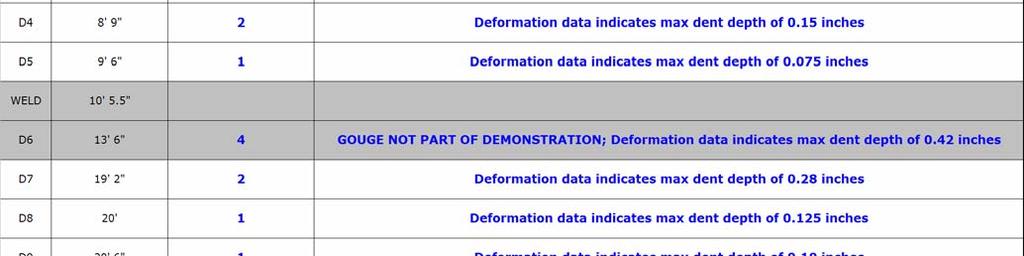
29 The benchmark data and test results for PNNL s PNNL Ultrasonic Strain Measurement technology are shown in Table 8 and Table 9. Table 8. Benchmark vs. Test Results for Mechanical Damage Pipe Sample 1 PIPE SAMPLE 1 Dent Severity = No damage Search 1 = Least Severe Defect Region 2 = Moderately Severe Number (from End A) 3 = Severe Comments 4 = Most Severe Benchmark PNNL D dent start at 63.5" end at 66.5", length 3" D dent start at 67" end at 7", length 3" D dent start at 77.3" end at 78.1", length.9" D long dent along the axis dent start at 99.9" end at 11.4", length 1.5" D long dent along the axis dent start at 113.8" end at 119.9", D Not Part of Benchmark length 6.1" detected, damage looks as significant as a 3 or 4, length approximately 6 inches long or two dents approximately 2 inches long separated by 1 inch damage detected; damage looks as significant as a 3, (1 defect approximately 7 inches long or 2 defects, one 4 inches long and a second 2 inches long separated by approximately 1 inch) D dent start at 228.1" end at 234.7", length 6.7" D dent start at 236.4" end at length 5.7" D dent start at 245.7" end at 246.2", length.5" D D D D NR out of scan range D NR out of scan range D NR out of scan range similar to calibration defects dent start at 264" end at 27.1", length 6.1" similar to calibration defects dent start at 271" end at length 5.1" similar to calibration defects dent start at 277.3" end at 282.6", length 5.3" 28

30 Table 9. Benchmark vs. Test Results for Mechanical Damage Pipe Sample 2 PIPE SAMPLE 2 Dent Severity = No damage Search Defect 1 = Least Severe Region Number 2 = Moderately Severe (from End A) 3 = Most Severe Comments Benchmark PNNL R " 1 1 small degree of damage, start of dent 17" end 11" length 3" R moderate damage, start of dent 14.25" end 147.5", length 7.25" R significant damage, start of dent " end , length 8.5 R small degree of localized damage, start of dent 215.5" end 22, length 4.5" R moderate damage, start of dent 25.5" end 258.5, length 8" R significant damage, start of dent end , length 8.5" R moderate damage, start of dent 323" end 331", length 8" R significant damage, start of dent 359" end 367", length 8" R no dent The term dent severity is used in this report to describe relative severity of dents within a specific pipe sample. The absolute severity of each dent is not known. Determining the severity of mechanical damage is difficult since there are no standards such as those used for corrosion anomalies. The criteria used to establish the benchmark severity ratings could differ from PNNL s severity criteria and as such may have led to the discrepancies. PNNL began testing the afternoon of Monday January 1, 26 and completed testing by the afternoon of Friday January 13, 26. The PNNL Ultrasonic Strain Measurement technology only assesses the relative severity of mechanical damage defects. Location of dents is more practically performed by caliper tools and as such was not part of the evaluation criteria for this technology. Additionally, because PNNL was only required to identify dent severity at a specific location the scan speed was also not assessed. PNNL s technology performed well on the mechanical damage sample with plain dents (Pipe Sample 2). There was discrepancy between the PNNL data and the benchmark at defect sites R4 and R5 on Pipe Sample 2; however the remaining defect locations correlated well. There were a number of differences between the benchmark data and the PNNL data for Pipe Sample 1. PNNL noted that the multiple dents and the non-circular nature of the pipe from the three rows of dent defects on Pipe Sample 1 created a significant amount of background deformation and thus stress and strain within the pipe sample. Due to these factors, the PNNL Ultrasonic Strain Measurement technology was not optimized for the degree of background deformation and is possibly the reason for the discrepancies between the benchmark data and PNNL s results. PNNL indicated that additional tests would be desirable to help classify the dent severity for Pipe Sample 1. 29

31 Stress Corrosion Cracking Only one technology, the ORNL Shear Horizontal EMAT, was tested for detection of stress corrosion cracking. ORNL began testing the afternoon of Tuesday January 1, 26 and completed testing by mid-day Thursday January 12, 26. The ORNL Shear Horizontal EMAT technology acquired data as their inspection tool was continuously pulled through the pipe sample at the rate of about an inch per second. ORNL took multiple scans through each line to assess the consistency of the signal. Results were not displayed in real time; rather ORNL post processes the captured data to develop final results. ORNL claims post processing is minimal and could easily be performed during data acquisition with current generation computing power. As shown in Table 1 the technology ran three lines on a 26-inch diameter pipe with natural stress corrosion cracking. The EMAT technology detected one false positive signal on each test line. The configuration of the SCC defects could have contributed to the false positive readings. Because the EMAT configuration scans a minimum of 9-inches of the pipe s circumference, some of the false positives could be the result of other cracks located in close proximity to the SCC defects under evaluation. Only one defect site (SCC2) provided no discernable signal; however magnetic particle analysis showed that these cracks are small and difficult to detect. Additionally, the location of the crack colony listed as SCC3 is off by a couple of inches. This is possibly due to defect (18), not considered as part of the test and located approximately 3-inches away in the circumferential direction, which may have been detected over the smaller SCC colony in SCC3. The most significant cracks (SCC8, SCC9, and SCC1) in the test sample were detected by the ORNL Shear Horizontal EMAT technology. An example SCC defect is shown in Figure 21. The benchmark data and test results for ORNL s Shear Horizontal EMAT technology are shown in Table 1. Figure 21. Example SCC Defect 3

32 Table 1. Benchmark vs. ORNL Test Results; SCC Testing Defect Number SCC1 SCC2 (5 & 4) SCC3 (8) SCC4 SCC5 SCC6 SCC7 SCC8 (6) SCC9 (7) SCC1 (9) SCC11 (16) SCC12 SCC13 SCC14 Search Region (from End B) 242" to 254" 226" to 242" 21" to 222" 175" to 187" 14" to 152" 246" to 258" 234" to 246" 21" to 222" 188" to 2" 14" to 152" 225" to 245" 21" to 222" 188" to 2" 14" to 152" Start of Crack Region (from End B) Blank Benchmark End of Crack Region (from End B) Type of SCC Test Line Isolated Start of Crack Region (from End B) ORNL End of Crack Region (from End B) Type of SCC Colony Isolated Blank Blank Blank Test Line 2 Colony; another isolated at 142 Blank Isolated Colony Isolated Colony Colony Colony Test Line Colony Blank Blank Colony; looks like gap in the middle; may be 2 sets separated by 1-inch. Isolated; After scanning, we documented large dirt patches along line 3 We believe EMATs lifted off the surface due to dirt inside pipe. Reliability of data in this area is low Blank Isolated Polyethylene Pipe Defects Only one technology, the NETL Capacitive Sensor for Polyethylene Pipe Inspection, was tested for detection of plastic pipe defects. This technology inspects for small volumetric anomalies with an NETL specified detection threshold of approximately.15 cubic inches. The measurement technology is localized and therefore anomalies in close proximity and pipe end effects do not influence its detection capabilities. A measure of defect significance was established based on the calibration defect which was 3/8- inch in diameter and 5% deep (.28 cubic inches). The volume of the calibration defect was set at a significance of one. The significance of all other defects was based on the volume of the 31

33 calibration defect. An example defect is shown in Figure 22. This defect was calculated to have a volume of.4 cubic inches which equals a significance of As shown in Table 11, the technology ran one test line on a 6-inch diameter polyethylene pipe sample. Figure 22. Example Plastic Pipe Defect 32

34 Table 11. Benchmark vs. NETL Test Results; Plastic Pipe Testing Defect Number Search Region Defect Location from Side A (to center) Benchmark Significance of Defect (volume ratio from calibration defect) Defect Volume Defect Diameter Defect Location from Side A (to center) Significance of Defect (volume ratio from calibration defect) inches inches ratio in 3 inches inches ratio in 3 NETL Defect Volume Comments D1 21" to 27" For significance: defect calibration 18 = 1 18 =.28, 25.6 =.39 D2 28" to 34" Blank None D3 35" to 41" Blank None D4 42" to 48" Volume =.28 D5 49" to 55" /8 wide 1 long saw cut Volume =.37 D6 56" to 62" Blank None D7 62" to 7" Volume =.33 D8 7" to 76" Blank None D9 77" to 83" Blank None D1 84" to 9" Volume =.12 D11 91" to 97" Blank None D12 98" to 14" /8 wide 1 long saw cut Volume =.45 D13 15" to 111" Volume =.2 D14 112" to 118" Volume =.16 D15 119" to 125" 123 and (each).17 (each).25 (each) Volume =.21 D16 126" to 132" Blank None? Indications that a consistent amount of material may have been removed along entire length D17 132" to 138" Blank None? Indications that a consistent amount of material may have been removed along entire length D18 138" to 144" Volume =.32 D19 144" to 15" Volume =.2 Not part of the benchmarking demonstration 33

35 This page intentionally blank. 34

36 While this was the second demonstration for all other technology developers, this demonstration was the first for the NETL Capacitive Sensor technology and should be taken into consideration when evaluating the results. During the demonstration, the NETL Capacitive Sensor technology collected data at a frequency of 1-hertz but has the capability to collect data up to a frequency of 45-hertz. NETL s accuracy in assessing defect severity is depicted in Figure 23. The NETL Capacitive Sensor technology detection was excellent detecting all defect sites to within 1% of the actual centerline location and did not report any false positive signals. The percentage difference in defect significance was approximately 25% Predicted Significance Measured Significance Figure 23. Measured Severity vs. Predicted Severity for the NETL Capacitive Sensor SUMMARY Four pipeline anomaly conditions were evaluated by six different sensor technology developers. Three technologies assessed corrosion anomalies while individual technologies assessed mechanical damage, SCC, and plastic pipe material loss. The corrosion detection techniques demonstrated significant promise for inspection of unpiggable pipelines. Accurate detection and sizing of natural corrosion appears to be reachable 35

37 but additional development may be required to refine sizing algorithms especially when pipe material properties are unknown and calibration defects are not available. Additional data processing for some of the technologies and collection of larger natural corrosion defect libraries to conduct repeatable testing needs to be established. Future collection of data towards target corrosion on pipe samples pulled from service will improve system capabilities. In addition, the speed at which data is collected could be improved for all of the technologies. The usability of these technologies will rely on their ability to collect data for long pipeline segments in a relatively short amount of time as well as their ability to meet the design and power requirements of the Explorer robotic platform. PNNL s mechanical damage detection technique also achieved reasonably good results especially in the pipe sample containing only plain dents. Considering the uniqueness of Pipe Sample 1 (multiple dents in close proximity), more accurately assessing the dent severity for this type of pipe sample would be a future goal for PNNL s technology. In-service pipelines with the amount of denting evident on Pipe Sample 1 is highly unlikely and does not represent a realistic pipeline operating scenario. Track hoe defects; however, would be typical of third party damage evident on operating pipelines. The ORNL EMAT system also performed well detecting natural stress corrosion cracks that formed while the pipeline was in-service. The ORNL EMAT technology did detect some false positives on each test line but was also able to detect the most significant SCC locations. Given the nature of SCC, it is difficult to accurately size crack depths. Some of the cracks used in the benchmarking program may have been too small to clearly detect. Collection of additional SCC defect libraries and crack sizing would be a valuable addition to this benchmarking program. The NETL Capacitive Sensor was quite accurate in identifying defect locations. Sizing of plastic pipe defects is reachable but will require additional research to develop defect sizing algorithms. While this was a successful demonstration of the inspection sensor technology, inspection variables need to be considered in future evaluations. Following the submittal of their test data, the technology developers were sent the benchmark data. They were given an opportunity to comment on their results and to provide their perspective on their technology s performance relative to the benchmark data. Appendix C contains the developer s comments. Overall, the technologies performed well and the results are encouraging. As the development of these technologies progresses and future testing takes place, it is envisioned that improvements in the technology and data analysis techniques will continue to improve the false positive rate and enhance the precision and accuracy of the defect signals. PATH FORWARD As noted, PHMSA Pipeline Safety R&D Program goals are to understand the gaps between existing technologies and those needed to resolve the key pipeline issues. One recognized path forward is to integrate successfully demonstrated sensor technologies into a robotic platform/sensor system that can be deployed remotely as part of an integrated package. This effort is driven in large part by new PSIA regulations which require inspection of gas 36

38 transmission pipelines and distribution mains in high-consequence areas. A large percentage of these pipes cannot be inspected using typical smart-pig techniques because of diameter restrictions, pipe bends and valves. In addition, pressure differentials and flow can be too low to push a pig through some pipes. To help solve these problems, the PHMSA Pipeline Safety R&D Program has established an aggressive schedule to develop a prototype remote system which includes continued co-funding with industry partners. It is anticipated that upon completion of the prototype systems, they will be able to traverse all pipes (including unpiggable lines) of various diameters while providing continuous, real-time detection of pipe anomalies or defects. 37

39 This page intentionally blank. 38

40 APPENDIX A BENCHMARK DATA

41

42 Name: Date: Company: Sensor Design: Detection of Metal Loss - Page 1 Pipe Sample: Defect Set: Pipe Sample Calibration P1-1: Defect Search Region Start of Metal Loss Region Number (Distance from End B) from Side B P " to 64" CALIBRATION DATA Calibration Metal Loss Measured Length & Measured Max. Metal Loss Length & Width Depth of Metal Loss Location Width of Defect Depth of Defect inches from End B to center of defect inches inches PIPE SAMPLE 1: 361" (59" from End A) 2 x 2 See profile TEST DATA PIPE SAMPLE 1 8" Diameter,.188" Wall Thickness Pipe Sample; Schedule 1; Length = 34' 11.75" TEST LINE 1 End of Metal Loss Region Maximum Depth of Total Length of Metal Loss Region Width of Metal Loss Region from Side B Metal Loss Region inches inches inches inches inches inches Y/N Additional Data Attached? Comments Comments 56.75" 6.875" 4.125" 2".122" Y Defect 6 P " to 88" N BLANK 6 P1-1 1" to 112" N BLANK 5 WELD 12" P1-9 12" to 144" 12" 14.25" 2.25" Full Circumference.146" Y P1-NC1 P1-8 16" to 172" N BLANK 4 (natural corrosion pipe segment) WELD 18" P " to 196" " " 2.125" 2".147" Y Defect 5 P1-6 28" to 22" N BLANK 3 P " to 244" " " 3" 1".81" Y Defect 4 P " to 268" " " 4" 2".63" Y Defect 3 P1-3 28" to 292" " " 3.125" 2".96" Y Defect 2 P1-2 34" to 316" N BLANK 2 P " to 34" N BLANK 1 Defect Search Region Start of Metal Loss Region Number (Distance from End B) from Side B P1-23 TEST LINE 2 End of Metal Loss Region Maximum Depth of Total Length of Metal Loss Region Width of Metal Loss Region from Side B Metal Loss Region inches inches inches inches inches inches Y/N 74" to 86" 79.75" 83.75" 4" 2".97" Additional Data Attached? Y Comments Defect 11 P " to 11" 18" 11" 2" 2".12" Y Defect 1 WELD 12" P " to 144" 12" 14.75" P1-2 16" to 172" WELD 18" P " to 198" P " to 222" " " 2.75" Full Circumference.127" Y N N 4.25" 2".145" Y P1-NC2 BLANK 11 (natural corrosion pipe segment) BLANK 1 Defect 9 P " to 246" N BLANK 9 P " to 27" N BLANK 8 P " to 294" N BLANK 7 P " to 318" " 312" 3.125" 1".115" Y Defect 8 P " to 342" " " 3.875" 1.75".95" Y Defect 7 A-1

43 Name: Date: Company: Sensor Design: Benchmarking of Inspection Technologies Detection of Metal Loss - Page 2 CALIBRATION DATA Pipe Sample Calibration Metal Loss Location Metal Loss Length & Width Depth of Metal Loss inches from End B to center of defect inches inches PIPE SAMPLE 2: Calibration P2-1: 31.5" (58.5" from End A) 3 x 1 See profile Calibration P2-2: 275" (85" from End A) 2 x 2 See profile Measured Length & Width of Defect Measured Max. Depth of Defect Comments TEST DATA Pipe Sample: PIPE SAMPLE 2 Defect Set: 8" Diameter,.188" Wall Thickness Pipe Sample; Schedule 1; Length = 3'.375" TEST LINE 1 Defect Search Region Number (Distance from End B) Start of Metal Loss Region End of Metal Loss Region Maximum Depth of Total Length of Metal Loss Region Width of Metal Loss Region from Side B from Side B Metal Loss Region inches inches inches inches inches inches Y/N P " to 66" Additional Data Attached? N Comments BLANK 6 P2-1 78" to 9" 8.125" 84.5" 4.375" 2".147" Y Defect 5 P2-9 12" to 114" " " 4.125" 2".158" Y Defect 4 WELD 12" P " to 138" N BLANK 5 P2-7 15" to 162" " " 3.25" 1".85" Y Defect 3 P " to 186" 18.25" " 3.125" 1".114" Y Defect 2 P " to 21" N BLANK 4 P " to 234" " " 2.125" 2".79" Y P " to 258" N P2-2 27" to 282" N Defect 1 BLANK 3 BLANK 2 P " to 36" N BLANK 1 Start of Metal Loss Region End of Metal Loss Region Maximum Depth of Total Length of Metal Loss Region Width of Metal Loss Region from Side B from Side B Metal Loss Region inches inches inches inches inches inches Y/N Defect Search Region Number (Distance from End B) P2-2 54" to 66" 57.75" 6.875" TEST LINE " 1".188" Additional Data Attached? Y Comments Defect 11; through hole P " to 9" N BLANK 11 P " to 114" N BLANK 1 WELD 12" P " to 138" 13" " P " to 162" P " to 186" P " to 21" " 25.75" 4.125" 2".112" Y N N 3.125" 1".15" Y Defect 1 BLANK 9 BLANK 8 Defect 9 P " to 234" N BLANK 7 P " to 258" " 25.25" 2.125" 2".14" Y Defect 8 A-2

44 Name: Date: Company: Sensor Design: Benchmarking of Inspection Technologies Detection of Metal Loss - Page 3 CALIBRATION DATA Pipe Sample Calibration Metal Loss Location Metal Loss Length & Width Depth of Metal Loss inches from End B to center of defect inches inches PIPE SAMPLE 3: Calibration P3-1: 421" (59" from End A) 2 x 2 See profile Measured Length & Width of Defect Measured Max. Depth of Defect Comments TEST DATA Pipe Sample: PIPE SAMPLE 3 Defect Set: 8" Diameter,.188" Wall Thickness Pipe Sample; Schedule 1; Length = 4'.25" TEST LINE 1 End of Metal Loss Region Maximum Depth of Total Length of Metal Loss Region Width of Metal Loss Region from Side B Metal Loss Region inches inches inches inches inches inches Y/N Defect Search Region Start of Metal Loss Region Number (Distance from End B) from Side B P " to 78" Additional Data Attached? Comments N BLANK 5 P3-1 12" to 114" " " 3.25" 1".156" Y Defect 7 P " to 15" " ".67".67".12" N Defect 6; machined defect P " to 174" P " to 198" " 194" P " to 234" WELD 24" P3-5 27" to 282" 275" " P3-4 3" to 312" " " P3-3 33" to 342" 335" " P3-2 36" to 372" N 4.125" 2".115" Y N 2.25" 2".13" Y.75".75".148" N 2.25" 2".133" Y N BLANK 4 Defect 5 BLANK 3 Defect 4 Defect 3; machined defect Defect 2 BLANK 2 P " to 396" N BLANK 1 End of Metal Loss Region Maximum Depth of Total Length of Metal Loss Region Width of Metal Loss Region from Side B Metal Loss Region inches inches inches inches inches inches Y/N Defect Search Region Start of Metal Loss Region Number (Distance from End B) from Side B P " to 78" 69.5" " TEST LINE " 2".88" Additional Data Attached? Y Comments Defect 14 P " to 114" N BLANK 1 P " to 138" 13" " P " to 168" P " to 192" " " P " to 222" 214.5" " WELD 24" P " to 26" " " P " to 294" " 2".13" Y N.72".72".139" N 3.125" 1".91" Y 3.125" 1".7" Y N Defect 13 BLANK 9 Defect 12; machined defect Defect 11 Defect 1 BLANK 8 P " to 318" N BLANK 7 P " to 342" " ".75".75".154" N Defect 9; machined defect P " to 368" N BLANK 6 P " to 42" " " 4.125" 2".94" Y Defect 8 A-3

45 This page intentionally blank. A-4

46 A-5

47 This page intentionally blank. A-6

48 A-7

49 Name: Date: Company: Sensor Design: Benchmarking of Inspection Technologies Detection of SCC - Page 1 Pipe Sample: 993 Blank Area: Calibration Crack Location inches from end B Length Depth CALIBRATION DATA Measured Length Measured Depth Comments % wall inches thickness multiple cracks; max = ~3/4" multiple cracks; max = ~1/4" multiple cracks; max = ~3 1/4" multiple cracks; max = ~1/2" multiple cracks; max = ~1/2" Pipe Sample: Defect Set: Defect Number SCC5 (Blank 1) SCC4 (Blank 2) SCC3 (8) SCC2 (5 & 4) SCC1 (Blank 3) Search Region (Distance from End B) Start of Crack Region from Side B End of Crack Region from Side B inches inches inches 14" to 152" " to 187" " to 222" " to 242" " to 254" TEST DATA 26" Diameter Pipe with Stress Corrosion Cracks; Length = 26 feet Type of SCC Isolated Crack Colony of Cracks None Isolated Crack Colony of Cracks None Isolated Crack Colony of Cracks None Isolated Cracks Colony of Cracks None Isolated Crack Colony of Cracks None 893 TEST LINE 1 Comments Blank 1 Blank 2 Multiple 1/4" cracks; cracked area 2 3/4" by 2 1/2" Two isolated cracks; cracked area 4" by 1 1/2" with ~2" long crack; cracked area 5 1/4" by 1 1/4" with ~3" long crack Blank 3 A-8

50 Name: Date: Company: Sensor Design: Benchmarking of Inspection Technologies Detection of SCC - Page 2 TEST DATA Pipe Sample: 893 Defect Set: 26" Diameter Pipe with Stress Corrosion Cracks; Length = 26 feet Defect Number SCC1 (9) SCC9 (7) SCC8 (6) SCC7 (Blank 4) SCC6 (Blank 5) Search Region (Distance from End B) Start of Crack Region from Side B End of Crack Region from Side B inches inches inches 14" to 152" " to 2" " to 222" " to 246" " to 258" Type of SCC Isolated Crack Colony of Cracks None Isolated Crack Colony of Cracks None Isolated Crack Colony of Cracks None Isolated Crack Colony of Cracks None Isolated Crack Colony of Cracks None TEST LINE 2 Comments Multiple cracks; max ~1/4" long; cracked area 3 1/2" by 3 1/2" Multiple cracks; max ~1/4" long; cracked area 4 1/4" by 3 3/4" Multiple cracks; max ~1/2" long; cracked area 3" by 2 1/2" Blank Blank A-9

51 Name: Date: Company: Sensor Design: Benchmarking of Inspection Technologies Detection of SCC - Page 3 TEST DATA Pipe Sample: 893 Defect Set: 26" Diameter Pipe with Stress Corrosion Cracks; Length = 26 feet Defect Number SCC14 (Blank 6) SCC13 (Blank 7) SCC12 (Blank 8) SCC11 (16) Search Region (Distance from End B) Start of Crack Region from Side B End of Crack Region from Side B inches inches inches 14" to 152" " to 2" " to 222" " to 245" Type of SCC Isolated Crack Colony of Cracks None Isolated Crack Colony of Cracks None Isolated Crack Colony of Cracks None Isolated Crack Colony of Cracks None TEST LINE 3 Comments Blank Blank Blank Multiple cracks; max ~3/4" long; cracked area 17" by 1 3/4" A-1

52 Name: Date: Company: Sensor Design: Benchmarking of Inspection Technologies Detection of Plastic Pipe Defects - Page 1 CALIBRATION DATA Defect Calibration Defect Location Volume of Defect Depth of Defect Diameter of Defect inches from end A cubic inches inches inches C1: Comments Pipe Sample: Pipe Parameters: Defect Number Search Region (Distance from End A) inches Location of Defect Region from Side A inches Significance of Defect (based on volume ratio from calibration defect) Volume of Defect (in 3 ) (provided to participant after defect signif reported) Depth of Defect (in) (provided to participant after defect signif reported) Diameter of Defect (in) (provided to participant after defect signif reported) Calibration Defect = 1 Less Severe <1 More Severe >1 cubic inches inches inches D1 21" to 27" 25" TEST DATA PLASTIC PIPE SAMPLE 6" Diameter,.5" Wall Thickness Pipe Sample, ~13' in length LINE Comments D2 28" to 34" BLANK D3 35" to 41" BLANK D4 42" to 48" 46" D5 49" to 55" 53" Saw Cut ~1" long and 1/8" wide D6 56" to 62" BLANK D7 63" to 69" 67" D8 7" to 76" BLANK Same as D1 D9 77" to 83" BLANK D1 84" to 9" 88" D11 91" to 97" BLANK D12 98" to 14" 12" Saw Cut ~.9" long and 1/8" wide D13 15" to 111" 19" D14 112" to 118" 116" D15 119" to 125" 123" and 123.5".61 (each).17 (each).35 (each).25 (each) Defect consists of two identical holes 1/2" apart D16 126" to 132" BLANK D17 132" to 138" BLANK D18 138" to 144" 14" D19 144" to 15" 148" A-11

53 This page intentionally blank. A-12

54 APPENDIX B DEMONSTRATION TEST DATA

55

56 SOUTHWEST RESEARCH INSTITUTE (SWRI) DEMONSTRATION TEST DATA B-1

57 This page intentionally blank. B-2

58 Name: Date: Company: Sensor Design: Gary Burkhardt 27-Jan-6 Southwest Research Institute RFEC Benchmarking of Inspection Technologies Detection of Metal Loss - Page 1 Calibration P2-1: Calibration P2-2: Calibration P3-1: Pipe Sample: Defect Set: Pipe Sample Calibration P1-1: Defect Search Region Start of Metal Loss Region Number (Distance from End B) from Side B P " to 64" P " to 88" P1-1 1" to 112" WELD 12" CALIBRATION DATA Calibration Metal Loss Measured Length & Measured Max. Metal Loss Length & Width Depth of Metal Loss Location Width of Defect Depth of Defect inches from End B to center of defect inches inches PIPE SAMPLE 1: 359 (59 from End A) 2 x 2 See profile PIPE SAMPLE 2: (58.5 from End A) 3 x 1 See profile 277 (85 from End A) 2 x 2 See profile PIPE SAMPLE 3: (59 from End A) 2 x 2 See profile TEST DATA PIPE SAMPLE 1 8" Diameter,.188" Wall Thickness Pipe Sample; Schedule 1; Length = 34' 11.75" TEST LINE 1 End of Metal Loss Region Maximum Depth of Total Length of Metal Loss Region Width of Metal Loss Region from Side B Metal Loss Region inches inches inches inches inches inches Y/N Additional Data Attached? N Comments Comments No indication No indication P1-9 12" to 144" a=12, b=128.5 a=122.3, b=129.3 a=2.25, b=.77 a=1.82, b=full Circ. a=.66, b=.83 N Two defects in region, designated a and b. P1-8 16" to 172" Full Circ..18 N Appears to be large region of general wall thinning that extends out of the designated region. Signal patterns are not characteristic of the calibration defects. WELD 18" P " to 196" N P1-6 28" to 22" No indication P " to 244" N Defect type signal outside stated region. P " to 268" N P1-3 28" to 292" N P1-2 34" to 316" No indication P " to 34" No indication Defect Search Region Start of Metal Loss Region Number (Distance from End B) from Side B P1-23 P " to 11" WELD 12" End of Metal Loss Region Maximum Depth of Total Length of Metal Loss Region Width of Metal Loss Region from Side B Metal Loss Region inches inches inches inches inches inches Y/N 74" to 86" TEST LINE Additional Data Attached? N N Comments P " to 144" P1-2 16" to 172" WELD 18" P " to 198" P " to 222" P " to 246" P " to 27" P " to 294" P " to 318" P " to 342" Full Circ..6 N Full Circ..18 N N N N B-3 Appears to be large region of general wall thinning that extends out of the designated region. Signal patterns are not characteristic of the calibration defects. No indication No indication No indication No indication

59 B-4

60 B-5

61 This page intentionally blank. B-6

62 Comments on Tests Performed During Demonstration at Battelle: Phase II Benchmarking Emerging Pipeline Inspection Technologies January 9 13, 26 APPLICATION OF REMOTE-FIELD EDDY CURRENT (RFEC) TESTING TO INSPECTION OF UNPIGGABLE PIPELINES OTHER TRANSACTION AGREEMENT DTRS56-2-T-1 SwRI PROJECT PIPELINE AND HAZARDOUS MATERIALS SAFETY ADMNISTRATION U.S. DEPARTMENT OF TRANSPORTATION SOUTHWEST RESEARCH INSTITUTE January 26 Demonstration tests of the remote-field eddy current (RFEC) method for inspection of 8-inch pipe were performed by Southwest Research Institute (SwRI ). The target application of the inspection technology is to integrate it with the Explorer II robot under development by Carnegie Mellon University. Therefore, the approach taken by SwRI was to perform the demonstration using a tool that meets the requirements and specifications for the Explorer II robot. All of the instrumentation (except for external power, which will be supplied by the robot), including excitation signal generation, amplification, filtering, multiplexing, analog-to-digital conversion, and digital signal processing (to provide phase-sensitive signal detection), was located on the RFEC tool. Total power required was less than half of the power budget available from the robot. Communication of commands and transfer of the processed signal data to an external computer were accomplished using a CAN bus the same bus that will be used on the robot. Although the tool incorporated 8 channels (coverage of 6 degrees circumferentially) instead of the 48 channels intended for the robot tool (to achieve 36 degrees coverage), the circuitry is readily scalable to the full number of channels. Data were acquired by all 8 channels simultaneously during a single scan. The scans were made at a velocity of 1.5 inches/sec, and it was demonstrated that 4 inches/sec (the maximum scan speed of the robot) was possible. The data were post-processed for analysis to determine defect characteristics (length, width, and depth) using software that is readily adaptable to field inspections The development of hardware that meets constraints associated with factors such as scan speed, power, and size always results in compromises that are not factors if, for example, laboratory instrumentation is used and if scan speeds are very slow. For example, slow scan speeds mean that significantly greater noise-reduction filtering can be used because time constants can be very long compared to those necessitated by fast scan speeds. Laboratory instrumentation can incorporate additional filtering and signal processing that cannot readily be performed by circuitry that must meet size and power constraints. Since the SwRI tool met the robot constraints, it can be expected that results similar to those achieved in these tests can be expected from the final integrated hardware. B-7

63 It should be noted that defect characterization has a strong subjective element. In this demonstration, we were working with a brand new system, looking at defect types we had not seen before. That meant we had to use our best judgment and understanding of the RFEC method to interpret the indications. After the system has been used more extensively, experience will allow the operator to know quickly what type of defect is being detected based on the signal characteristics. The quantitative interpretation of the signals will then be improved over the present level. For example, the natural corrosion region in the demonstration pipes gave a signal unlike any of the calibration defects in our lab or supplied by Battelle. Furthermore, the signal extended beyond the designated region. As a result, we used our best judgment and reported the wall loss indicated by our depth algorithms. Magnetic field effects or the simple nature of RFEC response to very large area defects could cause our estimate to be in error. Familiarity with this type defect over a period of time would assure us of making a quicker and potentially more accurate appraisal of the corrosion. B-8

64 GAS TECHNOLOGY INSTITUTE (GTI) Demonstration Test Da Name: Date: Company: Sensor Design: Benchmarking of Inspection Technologies Detection of Metal Loss - Page 2 TEST DATA Pipe Sample: PIPE SAMPLE 2 Defect Set: 8" Diameter,.188" Wall Thickness Pipe Sample; Schedule 1; Length = 3'.375" TEST LINE 1 Defect Search Region Number (Distance from End B) P " to 66" P2-1 78" to 9" P2-9 12" to 114" WELD 12" Start of Metal Loss Region End of Metal Loss Region Maximum Depth of Total Length of Metal Loss Region Width of Metal Loss Region from Side B from Side B Metal Loss Region inches inches inches inches inches inches Y/N Additional Data Attached? Comments None P " to 138" P2-7 15" to 162" P " to 186" P " to 21" P " to 234" P " to 258" P2-2 27" to 282" P " to 36" None None None None None Defect Search Region Number (Distance from End B) P2-2 54" to 66" P " to 9" P " to 114" WELD 12" TEST LINE 2 Start of Metal Loss Region End of Metal Loss Region Maximum Depth of Total Length of Metal Loss Region Width of Metal Loss Region from Side B from Side B Metal Loss Region inches inches inches inches inches inches Y/N Additional Data Attached? Comments None None P " to 138" P " to 162" P " to 186" P " to 21" P " to 234" P " to 258" None None None B-9

65 B-1

66 Analysis of Sensor Benchmarking Tests Remote Field Eddy Current Technique Prepared by: Julie Maupin, Albert Teitsma, Paul Shuttleworth Gas Technology Institute 17 S. Mount Prospect Road Des Plaines, Illinois January 26 B-11

67 Abstract During the week of 9 January 26, GTI staff travelled to the Battelle Lab s West Jefferson facility in Columbus, OH to test a prototype RFEC inspection vehicle in 3 samples of 8 pipe. We report briefly on the apparatus and its design, the electronic readout and data acquisition, and the analysis of the data. Where appropriate, we have discussed effects which lead to uncertainties in the location and size of reported defects. We also discuss uncertainties which may affect whether a defect would have been observable by our apparatus. Introduction The remote field eddy current (RFEC) technique is an electromagnetic, through-wall inspection technique for detecting defects and wall thinning in pipe walls. A simple exciter coil can be driven with a low frequency sinusoidal current to generate an oscillating magnetic field that small sensor coils can detect. This low frequency (1 s of Hz) oscillating field will propagate via two paths. It will propagate directly down the pipe a short distance. It will also propagate out through the wall, along the exterior of the pipe, and will re-enter the pipe --- the so-called indirect field. At axial distances of 2-3 pipe diameters from the exciter coil, the indirect field re-entering the interior of the pipe is much larger than the direct field coming from the exciter coil. Since it passes through the pipe wall, the indirect field contains information regarding the condition of the pipe. Changes from nominal value of the amplitude and phase of the indirect field indicate defects in the wall. Figure 1: Paths of Energy Flow in the RFEC Technique. The remote field re-entering the pipe is the one containing the information regarding the condition of the pipe wall. We constructed a vehicle ( jig ) for carrying the RFEC apparatus. Near its front end it carried a solenoidal exciter coil, approximately 4 in diameter and 5 in length. It was comprised of13 windings of 26 gauge wire. The sensor coils are located at distances of approximately 17 upstream of the exciter coil. They are ¾ in diameter, 3/8 in width, and contain approximately 2K windings of 5 gauge wire. Configured on the jig as two sets of 8 sensor coils, each set covered an angle of approximately 6º circumferentially at ¼ spacing. Mechanical Design The RFEC vehicle was composed of three parts, front support, rear support, and the center body. The front and rear supports had steering mechanisms on the wheels that helped keep the device upright and prevented any major rotation of the vehicle. The supports were coupled to B-12

68 the center body, which contained all the equipment necessary to the RFEC technique. A picture of the center body is shown in Figure 2. MUX Board Mock Explorer Module Support Sensor Coils Drive Coil Figure 2: Center body of RFEC vehicle. GTI used two sets of 8 sensor coils to measure two defect lines simultaneously. The coils were mounted on shafts that served as pegs to attach the coils to plastic guides as shown in Figure 3. The guides were rounded to match the circumference of the pipe and routed on the leading edge to avoid jamming the welds. The guides were held against the pipe wall by spring-loaded, parallelogram configured arms. An end view of the sensor coil mounts is shown in Figure 4. Direction Of Travel Plastic Coil Guide Coil Shaft Figure 3: Diagram of sensor coils mounted to plastic guides. B-13

69 Mounting Spring Plastic Coil Figure 4: Sensor coil mounts inside an 8 pipe. The drive coil has been placed between two support modules, one having been built to imitate a module on the Explorer II robot. These support modules were important to keeping the drive coil centered in the pipe. GTI used an automatic winch system to pull the vehicle through the pipe. A tether line was attached to the front end of the vehicle. The tether wraps once around an encoder and then is wound onto a motor. The system is mounted directly onto the pipe and is controlled by LabVIEW to move the vehicle in ¼ steps. Uncertainties Related to Mechanics The jig suffered from some rotation inside the pipe. Each coil could have experienced rotations of up to ±1. There were some encoder losses. After traveling 25 in the pipe, we were measuring about 5 short of the actual location of the sensor coils. We eventually attached a fiberglass tape measure to the back end of the vehicle so we could always double check the encoder readings. In order to get good wall coverage from the coils, they had to be staggered, meaning half were closer to the drive coil than the other half. We have made provisions to correct the offset in the data analysis but there will still likely be an effect on the results. B-14

70 Electronics and Data Acquisition (DAQ) System GTI s embodiment of a Remote Field Eddy Current inspection system is as follows: Signal Recovery 7265 DSP lock-in amplifier, Kepco BOP36-6M excitation coil driver, ADG47 16 channel multiplexer, Ni GPIB+ Gpib board and Ni PCI-661 Counter Timer board. The preceding hardware is controlled by a Dell Pentium 4 workstation running at 2.99MHz with 1Gb of main memory and executing Lab View 7.1 under Windows XP Professional operating system. A general schematic of the DAQ system is shown in Figure 7. Channel addressing and distance gauging is accomplished using a Ni 661 time/counter PCI circuit board. Distance measurements are made using a relative incremental encoder having a resolution of 1/16. Figure 5: Schematic of DAQ System. This figure schematically shows a 4-channel system. The system we operated at Battelle was a 16-channel version of this schematic. GTI s RFEC machine is using a 1 count per revolution quadrature encoder. The encoder is interfaced to the system using a National Instrument PCI-661 counter/timer circuit board. This circuit board supports 5 encoders; the encoder interface is done in hardware. The counter chip used in the NI circuit board has 32 bit registers giving a counting range of 268,435,453 inch. Data Collection Three LabView programs were used to collect data from the instrumentation on the jig. One read the encoder, one controlled the motor, and the other controlled the lock-in amplifier and acquired data from the coils. Acquiring the phase angle and magnitude of each coil was achieved by using a sequence of binary addressing to the multiplexer board. The program cycles through each coil sequentially. Once the data has been acquired for all 16 coil channels, the motor program fires the motor until the encoder program realizes it has traveled to the next ¼ step. Once the motor stops, the coils are again read and the phase and magnitude data is recorded to Excel. The process repeats. The lock-in amplifier has a programmable time constant for the low pass filter at its output. The program was written so that the operator could set the number of time constants that the program would wait at each coil address. Having a wait of multiple time constants ensured that B-15

71 unsettled data would be flushed out and the readings would be accurate. The drawback to waiting for a certain number of time constants is slower acquisition time. It takes a significantly longer time to obtain data for 16 coils making overall inspection speed slow. No problems were encountered with LabVIEW. Analysis Pipe Sample 3 Analysis of defect depth on Pipe Sample 3 was primarily done using Russell NDE Systems Inc. s Adept Pro program. This program is the result of decades of research and focuses on the Voltage Plane for analysis. The display produced by the program is shown for Defect Line1 in Figure 6. B-16

72 Defects ϕ Weld Figure 6: Adept Pro display of Defect Line 1 from Pipe Sample 3. B-17

73 The display shows a strip chart of the phase angle on the left, followed by a C-Scan of the phase. Although the C-Scan provides a good overview of the defects, often as in this case, the strip chart is better for seeing the smaller defects. The magnitude information (strip chart and C- scan) is displayed to the right of the phase information. The top right hand panel shows the Voltage Plane. The black spiral is the attenuation spiral: as the wall thickness increases, the remote filed eddy current signal strength decreases while the phase also decreases, resulting in a spiral polar plot. The blue curve on the plot is the signal from the defect at the horizontal marker that runs across the strip charts and C-scans. The two red lines on either side of the marker delimit the range of data analyzed. If the blue line is extended to intersect the wall-thinning spiral, the vector from the origin of the polar plot to the intersection point makes an angle φ with the x-axis. Angle φ is used to determine the depth of the defect. The length of the blue line is used to find the circumferential extent of the defect. As in Figure 6, Figure 7 shows the analysis of Line 2 of Pipe 3. B-18

74 Defects Weld Figure 9: Adept Pro Display of Defect Line 2. Adept Pro s function is primarily to determine defect depth. Defect length and width are best obtained from axial and circumferential scans across the defect. Remote field eddy current signals spread in both the axial and the circumferential directions. To get length and width B-19

75 requires corrections for the spread. Axial lengths estimated from the data should be reasonable. However, the combination of much greater spread in the circumferential direction combined with sensor separation means circumferential precision is poor. Pipe 2 was analyzed with an internally written MATLAB program. The fundamental equations are the same as used by Russell s Adept Pro software but there are some differences in the calibration. This can lead to small differences in the results for this pipe. This approach was used because Pipe 2 has two calibration defects with different depths. We expect the new calibration to give better results over a wide range of defect depths. B-2

76 Table 1: C-scan Plots of defects found on Pipe 3 Test Line 1. P3-1 P3-9 P3-7 P3-5 P3-4 P3-3 B-21

77 Table 2: Line 1 Defects Defect Max Depth (% Location of wall thick.) Defect Length Defect Width 16 96% % % % % % C-Scan plots The C-scan plots for all found defects are attached as a separate document. The tables containing Pipe 1 defects show the strip chart and C-scan for the phase only. The tables containing Pipe 2 defects show the C-scan for the phase only. Finally, the tables containing Pipe 3 defect information show the strip chart and C-scan for both the phase and magnitude. Summary Results Table The Excel spreadsheet summarizing the results is attached as a separate document. Pipe 2 data was only analyzed for the deepest pit. Data from Pipes 1 and 3 that showed dual pits are recorded in the spreadsheet as two measurements representing the maximum depth of each pit. B-22

78 Table 1: C-scan Plots of defects found on Pipe 1 Test Line 1. P1-12 P1-9 P1-7 P1-5 P1-4 P1-3 B-23

79 P1-2 B-24

80 Table 2: C-scan Plots of defects found on Pipe 1 Test Line 2. P1-23 P1-22 P1-21 P1-18 P1-14 P1-13 B-25

81 Table 3: C-scan Plots of defects found on Pipe 2 Test Line 1. P2-1 P2-9 P2-7 P2-6 P2-4 B-26

82 Table 4: C-scan Plots of defects found on Pipe 2 Test Line 2. P2-2 P2-17 P2-14 P2-12 B-27

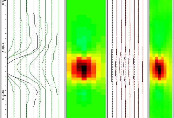
83 Table 5: C-scan Plots of defects found on Pipe 3 Test Line 1. P3-1 P3-9 P3-7 P3-5 P3-4 P3-3 B-28

84 Table 6: C-scan Plots of defects found on Pipe 3 Test Line 2. P3-23 P3-21 P3-19 P3-18 P3-17 P3-14 B-29

85 P3-12 B-3

86 BATTELLE DEMONSTRATION TEST DATA B-31

87 This page intentionally blank. B-32

88 Name: Date: Company: Sensor Design: Bruce Nestleroth January 26,26 Battelle Rotating Permanent Magnet Eddy Current Inspection System Benchmarking of Inspection Technologies Detection of Metal Loss - Page 1 Pipe Sample: Defect Set: Defect Search Region Number (Distance from End B) P " to 64" TEST DATA PIPE SAMPLE 1 8" Diameter,.188" Wall Thickness Pipe Sample; Schedule 1; Length = 34' 11.75" TEST LINE 1 Start of Metal Loss Region End of Metal Loss Region Total Length of Metal Loss Maximum Depth of Width of Metal Loss Region from Side B from Side B Region Metal Loss Region inches inches inches inches inches inches Y/N Additional Data Attached? Yes. Raw Signals Comments Corrosion patch, with multiple pits of different depths P " to 88" No Metal Loss Detected Yes. Raw Signals P1-1 1" to 112" WELD 12" No Metal Loss Detected Yes. Raw Signals P1-9 12" to 144" P1-8 16" to 172" WELD 18" No Metal Loss Detected Various depths up to.15 inches Yes. Raw Signals Yes. Raw Signals A large area of general corrosion of variable depth that spans the entire sensor width. The corrosion is close to the weld, altering both signals. A large wide corrosion area at 128" A slow change in signal in all sensors throughout the region indicates a material property change P " to 196" Yes. Raw Signals Corrosion patch, with multiple pits of different depths P1-6 28" to 22" No Metal Loss Detected Yes. Raw Signals P " to 244" Yes. Raw Signals Corrosion patch, with multiple pits of different depths P " to 268" Yes. Raw Signals Corrosion patch, with multiple pits of different depths P1-3 28" to 292" Yes. Raw Signals Corrosion patch, with multiple pits of different depths P1-2 34" to 316" No Metal Loss Detected Yes. Raw Signals P " to 34" No Metal Loss Detected Yes. Raw Signals Defect Search Region Number (Distance from End B) P " to 86" TEST LINE 2 Start of Metal Loss Region End of Metal Loss Region Total Length of Metal Loss Maximum Depth of Width of Metal Loss Region from Side B from Side B Region Metal Loss Region inches inches inches inches inches inches Y/N Additional Data Attached? Yes. Raw Signals Comments Corrosion patch, with multiple pits of different depths P " to 11" Yes. Raw Signals Corrosion patch, with multiple pits of different depths WELD 12" P " to 144" P1-2 16" to 172" No Metal Loss Detected Greater than 5 inches Various depths up to.15 inches Yes. Raw Signals Yes. Raw Signals A area of general corrosion of variable depth that spans most sensors. A large wide corrosion area at 128". A slow change in signal in all sensors throughout the region indicates a material property change WELD 18" P " to 198" No Metal Loss Detected Yes. Raw Signals P " to 222" Yes. Raw Signals Corrosion patch, with multiple pits of different depths P " to 246" Yes. Raw Signals Small single pit P " to 27" No Metal Loss Detected Yes. Raw Signals P " to 294" No Metal Loss Detected Yes. Raw Signals P " to 318" Yes. Raw Signals Corrosion patch, with multiple pits of different depths P " to 342" Yes. Raw Signals Corrosion patch, with multiple pits of different depths B-33

89 B-34

90 B-35

91 This page intentionally blank. B-36

92 Pipe 1 Raw data output on same scale 42 inches, 2 12 and 18 inches Extra data for noise assessment Search Region Extra data for noise assessment Sensor Output Axial Sensors Radial Sensors CCW 2.5 CCW 2 CCW 1.5 CCW 1 CCW.5 deg CW.5 CW 1 CW1.5 CW 2 CW 2.5 CCW 2.5 CCW 2 CCW 1.5 CCW 1 CCW.5 deg CW.5 CW 1 CW1.5 CW 2 CW Distance (inches) Cal 1-1 Battelle Rotating Magnetic Field Inspection January 26 Pipe 1 - Page 1

93 Sensor Output Axial Sensors Radial Sensors CCW 2.5 CCW 2 CCW 1.5 CCW 1 CCW.5 deg CW.5 CW 1 CW1.5 CW 2 CW 2.5 CCW 2.5 CCW 2 CCW 1.5 CCW 1 CCW.5 deg CW.5 CW 1 CW1.5 CW 2 CW Distance (inches) P1-1 Sensor Output Axial Sensors Radial Sensors CCW 2.5 CCW 2 CCW 1.5 CCW 1 CCW.5 deg CW.5 CW 1 CW1.5 CW 2 CW 2.5 CCW 2.5 CCW 2 CCW 1.5 CCW 1 CCW.5 deg CW.5 CW 1 CW1.5 CW 2 CW Distance (inches) P1-2 Battelle Rotating Magnetic Field Inspection January 26 Pipe 1 - Page 2

94 Sensor Output Axial Sensors Radial Sensors CCW 2.5 CCW 2 CCW 1.5 CCW 1 CCW.5 deg CW.5 CW 1 CW1.5 CW 2 CW 2.5 CCW 2.5 CCW 2 CCW 1.5 CCW 1 CCW.5 deg CW.5 CW 1 CW1.5 CW 2 CW Distance (inches) P1-3 Sensor Output Axial Sensors Radial Sensors CCW 2.5 CCW 2 CCW 1.5 CCW 1 CCW.5 deg CW.5 CW 1 CW1.5 CW 2 CW 2.5 CCW 2.5 CCW 2 CCW 1.5 CCW 1 CCW.5 deg CW.5 CW 1 CW1.5 CW 2 CW Distance (inches) P1-4 Battelle Rotating Magnetic Field Inspection January 26 Pipe 1 - Page 3

95 Sensor Output Axial Sensors Radial Sensors CCW 2.5 CCW 2 CCW 1.5 CCW 1 CCW.5 deg CW.5 CW 1 CW1.5 CW 2 CW 2.5 CCW 2.5 CCW 2 CCW 1.5 CCW 1 CCW.5 deg CW.5 CW 1 CW1.5 CW 2 CW Distance (inches) P1-5 Sensor Output Axial Sensors Radial Sensors CCW 2.5 CCW 2 CCW 1.5 CCW 1 CCW.5 deg CW.5 CW 1 CW1.5 CW 2 CW 2.5 CCW 2.5 CCW 2 CCW 1.5 CCW 1 CCW.5 deg CW.5 CW 1 CW1.5 CW 2 CW Distance (inches) P1-6 Battelle Rotating Magnetic Field Inspection January 26 Pipe 1 - Page 4

96 Sensor Output Weld Signal Axial Sensors Radial Sensors CCW 2.5 CCW 2 CCW 1.5 CCW 1 CCW.5 deg CW.5 CW 1 CW1.5 CW 2 CW 2.5 CCW 2.5 CCW 2 CCW 1.5 CCW 1 CCW.5 deg CW.5 CW 1 CW1.5 CW 2 CW Distance (inches) P1-7 Sensor Output Weld Signal Axial Sensors Radial Sensors CCW 2.5 CCW 2 CCW 1.5 CCW 1 CCW.5 deg CW.5 CW 1 CW1.5 CW 2 CW 2.5 CCW 2.5 CCW 2 CCW 1.5 CCW 1 CCW.5 deg CW.5 CW 1 CW1.5 CW 2 CW Distance (inches) P1-8 Battelle Rotating Magnetic Field Inspection January 26 Pipe 1 - Page 5

97 Sensor Output Axial Sensors Radial Sensors CCW 2.5 CCW 2 CCW 1.5 CCW 1 CCW.5 deg CW.5 CW 1 CW1.5 CW 2 CW 2.5 CCW 2.5 CCW 2 CCW 1.5 CCW 1 CCW.5 deg CW.5 CW 1 CW1.5 CW 2 CW Distance (inches) P1-9 note reporting area larger, 12 to 144 inches Sensor Output Axial Sensors Radial Sensors Weld Signal CCW 2.5 CCW 2 CCW 1.5 CCW 1 CCW.5 deg CW.5 CW 1 CW1.5 CW 2 CW 2.5 CCW 2.5 CCW 2 CCW 1.5 CCW 1 CCW.5 deg CW.5 CW 1 CW1.5 CW 2 CW Distance (inches) P1-1 Battelle Rotating Magnetic Field Inspection January 26 Pipe 1 - Page 6

98 Sensor Output Axial Sensors Radial Sensors CCW 2.5 CCW 2 CCW 1.5 CCW 1 CCW.5 deg CW.5 CW 1 CW1.5 CW 2 CW 2.5 CCW 2.5 CCW 2 CCW 1.5 CCW 1 CCW.5 deg CW.5 CW 1 CW1.5 CW 2 CW Distance (inches) P1-11 Sensor Output Axial Sensors Radial Sensors CCW 2.5 CCW 2 CCW 1.5 CCW 1 CCW.5 deg CW.5 CW 1 CW1.5 CW 2 CW 2.5 CCW 2.5 CCW 2 CCW 1.5 CCW 1 CCW.5 deg CW.5 CW 1 CW1.5 CW 2 CW Distance (inches) 64 7 P1-12 Battelle Rotating Magnetic Field Inspection January 26 Pipe 1 - Page 7

99 Sensor Output Axial Sensors Radial Sensors CCW 2.5 CCW 2 CCW 1.5 CCW 1 CCW.5 18 deg CW.5 CW 1 CW1.5 CW 2 CW 2.5 CCW 2.5 CCW 2 CCW 1.5 CCW 1 CCW.5 18 deg CW.5 CW 1 CW1.5 CW 2 CW Distance (inches) P1-13 Sensor Output Axial Sensors Radial Sensors CCW 2.5 CCW 2 CCW 1.5 CCW 1 CCW.5 18 deg CW.5 CW 1 CW1.5 CW 2 CW 2.5 CCW 2.5 CCW 2 CCW 1.5 CCW 1 CCW.5 18 deg CW.5 CW 1 CW1.5 CW 2 CW Distance (inches) P1-14 Battelle Rotating Magnetic Field Inspection January 26 Pipe 1 - Page 8

100 Sensor Output Axial Sensors Radial Sensors CCW 2.5 CCW 2 CCW 1.5 CCW 1 CCW.5 18 deg CW.5 CW 1 CW1.5 CW 2 CW 2.5 CCW 2.5 CCW 2 CCW 1.5 CCW 1 CCW.5 18 deg CW.5 CW 1 CW1.5 CW 2 CW Distance (inches) P1-15 Sensor Output Axial Sensors Radial Sensors CCW 2.5 CCW 2 CCW 1.5 CCW 1 CCW.5 18 deg CW.5 CW 1 CW1.5 CW 2 CW 2.5 CCW 2.5 CCW 2 CCW 1.5 CCW 1 CCW.5 18 deg CW.5 CW 1 CW1.5 CW 2 CW Distance (inches) P1-16 Battelle Rotating Magnetic Field Inspection January 26 Pipe 1 - Page 9

101 Sensor Output Axial Sensors Radial Sensors CCW 2.5 CCW 2 CCW 1.5 CCW 1 CCW.5 18 deg CW.5 CW 1 CW1.5 CW 2 CW 2.5 CCW 2.5 CCW 2 CCW 1.5 CCW 1 CCW.5 18 deg CW.5 CW 1 CW1.5 CW 2 CW Distance (inches) P1-17 Sensor Output Axial Sensors Radial Sensors CCW 2.5 CCW 2 CCW 1.5 CCW 1 CCW.5 18 deg CW.5 CW 1 CW1.5 CW 2 CW 2.5 CCW 2.5 CCW 2 CCW 1.5 CCW 1 CCW.5 18 deg CW.5 CW 1 CW1.5 CW 2 CW Distance (inches) P1-18 Battelle Rotating Magnetic Field Inspection January 26 Pipe 1 - Page 1

102 Sensor Output Axial Sensors Radial Sensors CCW 2.5 CCW 2 CCW 1.5 CCW 1 CCW.5 18 deg CW.5 CW 1 CW1.5 CW 2 CW 2.5 CCW 2.5 CCW 2 CCW 1.5 CCW 1 CCW.5 18 deg CW.5 CW 1 CW1.5 CW 2 CW Distance (inches) P1-19 Sensor Output Axial Sensors Radial Sensors CCW 2.5 CCW 2 CCW 1.5 CCW 1 CCW.5 18 deg CW.5 CW 1 CW1.5 CW 2 CW 2.5 CCW 2.5 CCW 2 CCW 1.5 CCW 1 CCW.5 18 deg CW.5 CW 1 CW1.5 CW 2 CW Distance (inches) P1-2 Battelle Rotating Magnetic Field Inspection January 26 Pipe 1 - Page 11

103 Sensor Output Weld Signal Axial Sensors Radial Sensors CCW 2.5 CCW 2 CCW 1.5 CCW 1 CCW.5 18 deg CW.5 CW 1 CW1.5 CW 2 CW 2.5 CCW 2.5 CCW 2 CCW 1.5 CCW 1 CCW.5 18 deg CW.5 CW 1 CW1.5 CW 2 CW Distance (inches) P1-21 note reporting area larger, 12 to 144 inches Sensor Output Axial Sensors Radial Sensors Weld Signal CCW 2.5 CCW 2 CCW 1.5 CCW 1 CCW.5 18 deg CW.5 CW 1 CW1.5 CW 2 CW 2.5 CCW 2.5 CCW 2 CCW 1.5 CCW 1 CCW.5 18 deg CW.5 CW 1 CW1.5 CW 2 CW Distance (inches) P1-22 Battelle Rotating Magnetic Field Inspection January 26 Pipe 1 - Page 12

104 Sensor Output Axial Sensors Radial Sensors CCW 2.5 CCW 2 CCW 1.5 CCW 1 CCW.5 18 deg CW.5 CW 1 CW1.5 CW 2 CW 2.5 CCW 2.5 CCW 2 CCW 1.5 CCW 1 CCW.5 18 deg CW.5 CW 1 CW1.5 CW 2 CW 2.5 Distance (inches) P1-23 Battelle Rotating Magnetic Field Inspection January 26 Pipe 1 - Page 13

105 Pipe 2 Raw data output on same scale 36 inches,1 inches Extra data for noise assessment Search Region Extra data for noise assessment Sensor Output Axial Sensors Radial Sensors CCW 2.5 CCW 2 CCW 1.5 CCW 1 CCW.5 18 deg CW.5 CW 1 CW1.5 CW 2 CW 2.5 CCW 2.5 CCW 2 CCW 1.5 CCW 1 CCW.5 18 deg CW.5 CW 1 CW1.5 CW 2 CW Distance (inches) Cal 2-1 Battelle Rotating Magnetic Field Inspection January 26 Pipe 2 - Page 1

106 Sensor Output Axial Sensors Radial Sensors CCW 2.5 CCW 2 CCW 1.5 CCW 1 CCW.5 18 deg CW.5 CW 1 CW1.5 CW 2 CW 2.5 CCW 2.5 CCW 2 CCW 1.5 CCW 1 CCW.5 18 deg CW.5 CW 1 CW1.5 CW 2 CW Distance (inches) Cal 2-2 Sensor Output Axial Sensors Radial Sensors CCW 2.5 CCW 2 CCW 1.5 CCW 1 CCW.5 deg CW.5 CW 1 CW1.5 CW 2 CW 2.5 CCW 2.5 CCW 2 CCW 1.5 CCW 1 CCW.5 deg CW.5 CW 1 CW1.5 CW 2 CW Distance (inches) P2-1 Battelle Rotating Magnetic Field Inspection January 26 Pipe 2 - Page 2

107 Sensor Output Axial Sensors Radial Sensors CCW 2.5 CCW 2 CCW 1.5 CCW 1 CCW.5 deg CW.5 CW 1 CW1.5 CW 2 CW 2.5 CCW 2.5 CCW 2 CCW 1.5 CCW 1 CCW.5 deg CW.5 CW 1 CW1.5 CW 2 CW Distance (inches) P2-2 Sensor Output Axial Sensors Radial Sensors CCW 2.5 CCW 2 CCW 1.5 CCW 1 CCW.5 deg CW.5 CW 1 CW1.5 CW 2 CW 2.5 CCW 2.5 CCW 2 CCW 1.5 CCW 1 CCW.5 deg CW.5 CW 1 CW1.5 CW 2 CW Distance (inches) P2-3 Battelle Rotating Magnetic Field Inspection January 26 Pipe 2 - Page 3

108 Sensor Output Axial Sensors Radial Sensors CCW 2.5 CCW 2 CCW 1.5 CCW 1 CCW.5 deg CW.5 CW 1 CW1.5 CW 2 CW 2.5 CCW 2.5 CCW 2 CCW 1.5 CCW 1 CCW.5 deg CW.5 CW 1 CW1.5 CW 2 CW Distance (inches) P2-4 Sensor Output Axial Sensors Radial Sensors CCW 2.5 CCW 2 CCW 1.5 CCW 1 CCW.5 deg CW.5 CW 1 CW1.5 CW 2 CW 2.5 CCW 2.5 CCW 2 CCW 1.5 CCW 1 CCW.5 deg CW.5 CW 1 CW1.5 CW 2 CW Distance (inches) P2-5 Battelle Rotating Magnetic Field Inspection January 26 Pipe 2 - Page 4

109 Sensor Output Axial Sensors Radial Sensors CCW 2.5 CCW 2 CCW 1.5 CCW 1 CCW.5 deg CW.5 CW 1 CW1.5 CW 2 CW 2.5 CCW 2.5 CCW 2 CCW 1.5 CCW 1 CCW.5 deg CW.5 CW 1 CW1.5 CW 2 CW Distance (inches) P2-6 Sensor Output Axial Sensors Radial Sensors CCW 2.5 CCW 2 CCW 1.5 CCW 1 CCW.5 deg CW.5 CW 1 CW1.5 CW 2 CW 2.5 CCW 2.5 CCW 2 CCW 1.5 CCW 1 CCW.5 deg CW.5 CW 1 CW1.5 CW 2 CW Distance (inches) P2-7 Battelle Rotating Magnetic Field Inspection January 26 Pipe 2 - Page 5

110 Sensor Output Weld Signal Axial Sensors Radial Sensors CCW 2.5 CCW 2 CCW 1.5 CCW 1 CCW.5 deg CW.5 CW 1 CW1.5 CW 2 CW 2.5 CCW 2.5 CCW 2 CCW 1.5 CCW 1 CCW.5 deg CW.5 CW 1 CW1.5 CW 2 CW Distance (inches) P2-8 Sensor Output P2-9 Signal Axial Sensors Radial Sensors CCW 2.5 CCW 2 CCW 1.5 CCW 1 CCW.5 deg CW.5 CW 1 CW1.5 CW 2 CW 2.5 CCW 2.5 CCW 2 CCW 1.5 CCW 1 CCW.5 deg CW.5 CW 1 CW1.5 CW 2 CW Distance (inches) P2-Weld Battelle Rotating Magnetic Field Inspection January 26 Pipe 2 - Page 6

111 Sensor Output Axial Sensors Radial Sensors CCW 2.5 CCW 2 CCW 1.5 CCW 1 CCW.5 deg CW.5 CW 1 CW1.5 CW 2 CW 2.5 CCW 2.5 CCW 2 CCW 1.5 CCW 1 CCW.5 deg CW.5 CW 1 CW1.5 CW 2 CW Distance (inches) P2-9 Sensor Output Axial Sensors Radial Sensors CCW 2.5 CCW 2 CCW 1.5 CCW 1 CCW.5 deg CW.5 CW 1 CW1.5 CW 2 CW 2.5 CCW 2.5 CCW 2 CCW 1.5 CCW 1 CCW.5 deg CW.5 CW 1 CW1.5 CW 2 CW Distance (inches) 9 96 P2-1 Battelle Rotating Magnetic Field Inspection January 26 Pipe 2 - Page 7

112 Sensor Output Axial Sensors Radial Sensors CCW 2.5 CCW 2 CCW 1.5 CCW 1 CCW.5 deg CW.5 CW 1 CW1.5 CW 2 CW 2.5 CCW 2.5 CCW 2 CCW 1.5 CCW 1 CCW.5 deg CW.5 CW 1 CW1.5 CW 2 CW Distance (inches) P2-11 Sensor Output Axial Sensors Radial Sensors CCW 2.5 CCW 2 CCW 1.5 CCW 1 CCW.5 deg CW.5 CW 1 CW1.5 CW 2 CW 2.5 CCW 2.5 CCW 2 CCW 1.5 CCW 1 CCW.5 deg CW.5 CW 1 CW1.5 CW 2 CW Distance (inches) P2-12 Battelle Rotating Magnetic Field Inspection January 26 Pipe 2 - Page 8

113 Sensor Output Axial Sensors Radial Sensors CCW 2.5 CCW 2 CCW 1.5 CCW 1 CCW.5 deg CW.5 CW 1 CW1.5 CW 2 CW 2.5 CCW 2.5 CCW 2 CCW 1.5 CCW 1 CCW.5 deg CW.5 CW 1 CW1.5 CW 2 CW Distance (inches) P2-13 Sensor Output Axial Sensors Radial Sensors CCW 2.5 CCW 2 CCW 1.5 CCW 1 CCW.5 deg CW.5 CW 1 CW1.5 CW 2 CW 2.5 CCW 2.5 CCW 2 CCW 1.5 CCW 1 CCW.5 deg CW.5 CW 1 CW1.5 CW 2 CW Distance (inches) P2-14 Battelle Rotating Magnetic Field Inspection January 26 Pipe 2 - Page 9

114 Sensor Output Axial Sensors Radial Sensors CCW 2.5 CCW 2 CCW 1.5 CCW 1 CCW.5 deg CW.5 CW 1 CW1.5 CW 2 CW 2.5 CCW 2.5 CCW 2 CCW 1.5 CCW 1 CCW.5 deg CW.5 CW 1 CW1.5 CW 2 CW Distance (inches) P2-15 Sensor Output Axial Sensors Radial Sensors CCW 2.5 CCW 2 CCW 1.5 CCW 1 CCW.5 deg CW.5 CW 1 CW1.5 CW 2 CW 2.5 CCW 2.5 CCW 2 CCW 1.5 CCW 1 CCW.5 deg CW.5 CW 1 CW1.5 CW 2 CW Distance (inches) P2-16 Battelle Rotating Magnetic Field Inspection January 26 Pipe 2 - Page 1

115 Sensor Output Weld Signal Axial Sensors Radial Sensors CCW 2.5 CCW 2 CCW 1.5 CCW 1 CCW.5 deg CW.5 CW 1 CW1.5 CW 2 CW 2.5 CCW 2.5 CCW 2 CCW 1.5 CCW 1 CCW.5 deg CW.5 CW 1 CW1.5 CW 2 CW Distance (inches) P2-17 Sensor Output Axial Sensors Radial Sensors CCW 2.5 CCW 2 CCW 1.5 CCW 1 CCW.5 deg CW.5 CW 1 CW1.5 CW 2 CW 2.5 CCW 2.5 CCW 2 CCW 1.5 CCW 1 CCW.5 deg CW.5 CW 1 CW1.5 CW 2 CW Distance (inches) P2-18 Battelle Rotating Magnetic Field Inspection January 26 Pipe 2 - Page 11

116 Sensor Output Axial Sensors Radial Sensors CCW 2.5 CCW 2 CCW 1.5 CCW 1 CCW.5 deg CW.5 CW 1 CW1.5 CW 2 CW 2.5 CCW 2.5 CCW 2 CCW 1.5 CCW 1 CCW.5 deg CW.5 CW 1 CW1.5 CW 2 CW Distance (inches) 9 96 P2-19 Sensor Output Axial Sensors Radial Sensors CCW 2.5 CCW 2 CCW 1.5 CCW 1 CCW.5 deg CW.5 CW 1 CW1.5 CW 2 CW 2.5 CCW 2.5 CCW 2 CCW 1.5 CCW 1 CCW.5 deg CW.5 CW 1 CW1.5 CW 2 CW Distance (inches) P2-2 Battelle Rotating Magnetic Field Inspection January 26 Pipe 2 - Page 12

117 Pipe 3 Raw data output on same scale 48 inches, 1 24 inches Extra data for noise assessment Search Region Extra data for noise assessment Sensor Output Axial Sensors Radial Sensors CCW 2.5 CCW 2 CCW 1.5 CCW 1 CCW.5 deg CW.5 CW 1 CW1.5 CW 2 CW 2.5 CCW 2.5 CCW 2 CCW 1.5 CCW 1 CCW.5 deg CW.5 CW 1 CW1.5 CW 2 CW Distance (inches) Cal 3-1 Battelle Rotating Magnetic Field Inspection January 26 Pipe 3 - Page 1

118 Sensor Output Axial Sensors Radial Sensors CCW 2.5 CCW 2 CCW 1.5 CCW 1 CCW.5 deg CW.5 CW 1 CW1.5 CW 2 CW 2.5 CCW 2.5 CCW 2 CCW 1.5 CCW 1 CCW.5 deg CW.5 CW 1 CW1.5 CW 2 CW Distance (inches) P3-1 Sensor Output Axial Sensors Radial Sensors CCW 2.5 CCW 2 CCW 1.5 CCW 1 CCW.5 deg CW.5 CW 1 CW1.5 CW 2 CW 2.5 CCW 2.5 CCW 2 CCW 1.5 CCW 1 CCW.5 deg CW.5 CW 1 CW1.5 CW 2 CW Distance (inches) P3-2 Battelle Rotating Magnetic Field Inspection January 26 Pipe 3 - Page 2

119 Sensor Output Axial Sensors Radial Sensors CCW 2.5 CCW 2 CCW 1.5 CCW 1 CCW.5 deg CW.5 CW 1 CW1.5 CW 2 CW 2.5 CCW 2.5 CCW 2 CCW 1.5 CCW 1 CCW.5 deg CW.5 CW 1 CW1.5 CW 2 CW Distance (inches) P3-3 Sensor Output Axial Sensors Radial Sensors CCW 2.5 CCW 2 CCW 1.5 CCW 1 CCW.5 deg CW.5 CW 1 CW1.5 CW 2 CW 2.5 CCW 2.5 CCW 2 CCW 1.5 CCW 1 CCW.5 deg CW.5 CW 1 CW1.5 CW 2 CW Distance (inches) P3-4 Battelle Rotating Magnetic Field Inspection January 26 Pipe 3 - Page 3

120 Sensor Output Axial Sensors Radial Sensors CCW 2.5 CCW 2 CCW 1.5 CCW 1 CCW.5 deg CW.5 CW 1 CW1.5 CW 2 CW 2.5 CCW 2.5 CCW 2 CCW 1.5 CCW 1 CCW.5 deg CW.5 CW 1 CW1.5 CW 2 CW Distance (inches) P3-5 Sensor Output Axial Sensors Radial Sensors CCW 2.5 CCW 2 CCW 1.5 CCW 1 CCW.5 deg CW.5 CW 1 CW1.5 CW 2 CW 2.5 CCW 2.5 CCW 2 CCW 1.5 CCW 1 CCW.5 deg CW.5 CW 1 CW1.5 CW 2 CW Distance (inches) P3-Weld Battelle Rotating Magnetic Field Inspection January 26 Pipe 3 - Page 4

121 Sensor Output Axial Sensors Radial Sensors CCW 2.5 CCW 2 CCW 1.5 CCW 1 CCW.5 deg CW.5 CW 1 CW1.5 CW 2 CW 2.5 CCW 2.5 CCW 2 CCW 1.5 CCW 1 CCW.5 deg CW.5 CW 1 CW1.5 CW 2 CW Distance (inches) P3-6 Sensor Output Axial Sensors Radial Sensors CCW 2.5 CCW 2 CCW 1.5 CCW 1 CCW.5 deg CW.5 CW 1 CW1.5 CW 2 CW 2.5 CCW 2.5 CCW 2 CCW 1.5 CCW 1 CCW.5 deg CW.5 CW 1 CW1.5 CW 2 CW Distance (inches) P3-7 Battelle Rotating Magnetic Field Inspection January 26 Pipe 3 - Page 5

122 Sensor Output Axial Sensors Radial Sensors CCW 2.5 CCW 2 CCW 1.5 CCW 1 CCW.5 deg CW.5 CW 1 CW1.5 CW 2 CW 2.5 CCW 2.5 CCW 2 CCW 1.5 CCW 1 CCW.5 deg CW.5 CW 1 CW1.5 CW 2 CW Distance (inches) P3-8 Sensor Output Axial Sensors Radial Sensors CCW 2.5 CCW 2 CCW 1.5 CCW 1 CCW.5 deg CW.5 CW 1 CW1.5 CW 2 CW 2.5 CCW 2.5 CCW 2 CCW 1.5 CCW 1 CCW.5 deg CW.5 CW 1 CW1.5 CW 2 CW Distance (inches) P3-9 Battelle Rotating Magnetic Field Inspection January 26 Pipe 3 - Page 6

123 Sensor Output Axial Sensors Radial Sensors CCW 2.5 CCW 2 CCW 1.5 CCW 1 CCW.5 deg CW.5 CW 1 CW1.5 CW 2 CW 2.5 CCW 2.5 CCW 2 CCW 1.5 CCW 1 CCW.5 deg CW.5 CW 1 CW1.5 CW 2 CW Distance (inches) P3-1 Sensor Output Axial Sensors Radial Sensors CCW 2.5 CCW 2 CCW 1.5 CCW 1 CCW.5 deg CW.5 CW 1 CW1.5 CW 2 CW 2.5 CCW 2.5 CCW 2 CCW 1.5 CCW 1 CCW.5 deg CW.5 CW 1 CW1.5 CW 2 CW Distance (inches) P3-11 Battelle Rotating Magnetic Field Inspection January 26 Pipe 3 - Page 7

124 Sensor Output Axial Sensors Radial Sensors CCW 2.5 CCW 2 CCW 1.5 CCW 1 CCW.5 18 deg CW.5 CW 1 CW1.5 CW 2 CW 2.5 CCW 2.5 CCW 2 CCW 1.5 CCW 1 CCW.5 18 deg CW.5 CW 1 CW1.5 CW 2 CW Distance (inches) P3-12 Sensor Output Axial Sensors Radial Sensors CCW 2.5 CCW 2 CCW 1.5 CCW 1 CCW.5 18 deg CW.5 CW 1 CW1.5 CW 2 CW 2.5 CCW 2.5 CCW 2 CCW 1.5 CCW 1 CCW.5 18 deg CW.5 CW 1 CW1.5 CW 2 CW Distance (inches) P3-13 Battelle Rotating Magnetic Field Inspection January 26 Pipe 3 - Page 8

125 Sensor Output Axial Sensors Radial Sensors CCW 2.5 CCW 2 CCW 1.5 CCW 1 CCW.5 18 deg CW.5 CW 1 CW1.5 CW 2 CW 2.5 CCW 2.5 CCW 2 CCW 1.5 CCW 1 CCW.5 18 deg CW.5 CW 1 CW1.5 CW 2 CW Distance (inches) P3-14 Sensor Output Axial Sensors Radial Sensors CCW 2.5 CCW 2 CCW 1.5 CCW 1 CCW.5 18 deg CW.5 CW 1 CW1.5 CW 2 CW 2.5 CCW 2.5 CCW 2 CCW 1.5 CCW 1 CCW.5 18 deg CW.5 CW 1 CW1.5 CW 2 CW Distance (inches) P3-15 Battelle Rotating Magnetic Field Inspection January 26 Pipe 3 - Page 9

126 Sensor Output Axial Sensors Radial Sensors CCW 2.5 CCW 2 CCW 1.5 CCW 1 CCW.5 18 deg CW.5 CW 1 CW1.5 CW 2 CW 2.5 CCW 2.5 CCW 2 CCW 1.5 CCW 1 CCW.5 18 deg CW.5 CW 1 CW1.5 CW 2 CW Distance (inches) P3-16 Sensor Output Axial Sensors Radial Sensors CCW 2.5 CCW 2 CCW 1.5 CCW 1 CCW.5 18 deg CW.5 CW 1 CW1.5 CW 2 CW 2.5 CCW 2.5 CCW 2 CCW 1.5 CCW 1 CCW.5 18 deg CW.5 CW 1 CW1.5 CW 2 CW Distance (inches) P3-17 Battelle Rotating Magnetic Field Inspection January 26 Pipe 3 - Page 1

127 Sensor Output Axial Sensors Radial Sensors CCW 2.5 CCW 2 CCW 1.5 CCW 1 CCW.5 18 deg CW.5 CW 1 CW1.5 CW 2 CW 2.5 CCW 2.5 CCW 2 CCW 1.5 CCW 1 CCW.5 18 deg CW.5 CW 1 CW1.5 CW 2 CW Distance (inches) P3-Weld Sensor Output Axial Sensors Radial Sensors CCW 2.5 CCW 2 CCW 1.5 CCW 1 CCW.5 18 deg CW.5 CW 1 CW1.5 CW 2 CW 2.5 CCW 2.5 CCW 2 CCW 1.5 CCW 1 CCW.5 18 deg CW.5 CW 1 CW1.5 CW 2 CW Distance (inches) P3-18 Battelle Rotating Magnetic Field Inspection January 26 Pipe 3 - Page 11

128 Sensor Output Axial Sensors Radial Sensors CCW 2.5 CCW 2 CCW 1.5 CCW 1 CCW.5 18 deg CW.5 CW 1 CW1.5 CW 2 CW 2.5 CCW 2.5 CCW 2 CCW 1.5 CCW 1 CCW.5 18 deg CW.5 CW 1 CW1.5 CW 2 CW Distance (inches) P3-19 Sensor Output Axial Sensors Radial Sensors CCW 2.5 CCW 2 CCW 1.5 CCW 1 CCW.5 18 deg CW.5 CW 1 CW1.5 CW 2 CW 2.5 CCW 2.5 CCW 2 CCW 1.5 CCW 1 CCW.5 18 deg CW.5 CW 1 CW1.5 CW 2 CW Distance (inches) P3-2 Battelle Rotating Magnetic Field Inspection January 26 Pipe 3 - Page 12

129 Sensor Output Axial Sensors Radial Sensors CCW 2.5 CCW 2 CCW 1.5 CCW 1 CCW.5 18 deg CW.5 CW 1 CW1.5 CW 2 CW 2.5 CCW 2.5 CCW 2 CCW 1.5 CCW 1 CCW.5 18 deg CW.5 CW 1 CW1.5 CW 2 CW Distance (inches) P3-21 Sensor Output Axial Sensors Radial Sensors CCW 2.5 CCW 2 CCW 1.5 CCW 1 CCW.5 18 deg CW.5 CW 1 CW1.5 CW 2 CW 2.5 CCW 2.5 CCW 2 CCW 1.5 CCW 1 CCW.5 18 deg CW.5 CW 1 CW1.5 CW 2 CW Distance (inches) P3-22 Battelle Rotating Magnetic Field Inspection January 26 Pipe 3 - Page 13

130 Sensor Output Axial Sensors Radial Sensors CCW 2.5 CCW 2 CCW 1.5 CCW 1 CCW.5 18 deg CW.5 CW 1 CW1.5 CW 2 CW 2.5 CCW 2.5 CCW 2 CCW 1.5 CCW 1 CCW.5 18 deg CW.5 CW 1 CW1.5 CW 2 CW Distance (inches) P3-23 Battelle Rotating Magnetic Field Inspection January 26 Pipe 3 - Page 14

131 This page intentionally blank. B-76

132 PACIFIC NORTHWEST NATIONAL LABORATORY (PNNL) DEMONSTRATION TEST DATA B-77

133 This page intentionally blank. B-78

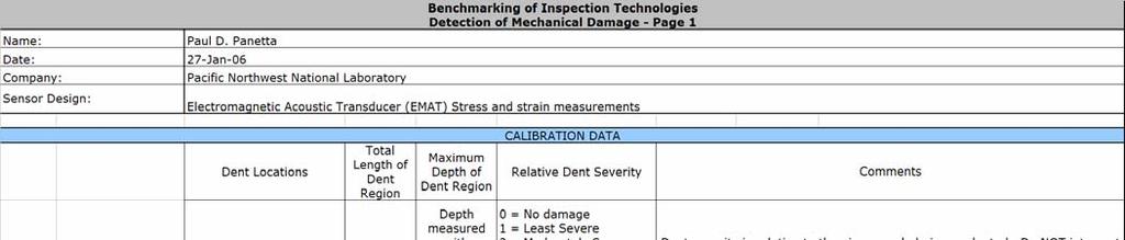
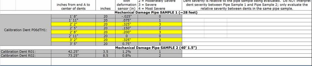
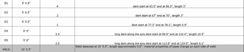
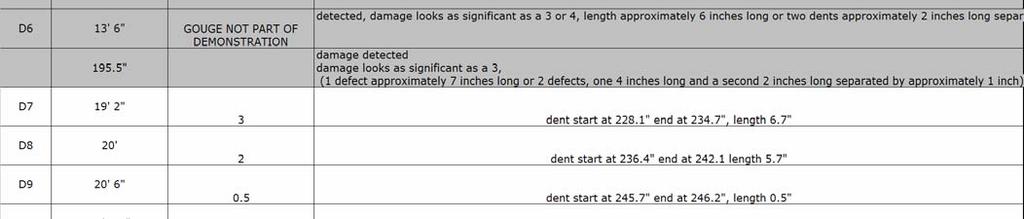
134 B-79

135 This page intentionally blank. B-8

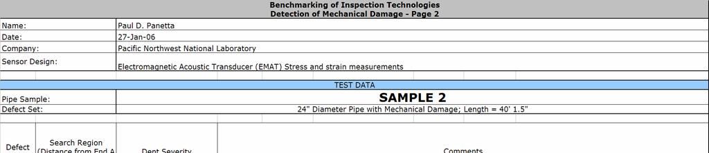
136 B-81

137 PNNL Ultrasonic measurements along the axis on Pipe 2, R Defects, at 15 degrees (approximately 3 ) from TDC 7.5 Ultrasonic Amplitude Spherical Cylindrical 1 Spherical Spherical No dent Ultrasonic birefringence Amplitude Ultrasonic thickness independent measurement Distance (inches) -.1 B-82

138 OAKRIDGE NATIONAL LABORATORY (ORNL) DEMONSTRATION TEST DATA B-83

139 This page intentionally blank. B-84

140 Name: Date: Company: Sensor Design: Benchmarking of Inspection Technologies Detection of SCC - Page 1 Venugopal K. Varma, Austion Albrught, and Philip Bingham 1/27/26 Oak Ridge National Laboratory EMAT shear Horizontal wave design Pipe Sample: Blank Area: Calibration Crack Location inches from end B Length Depth CALIBRATION DATA Measured Length Measured Depth Comments % wall inches thickness multiple cracks; max = ~3/4" multiple cracks; max = ~1/4" multiple cracks; max = ~3 1/4" multiple cracks; max = ~1/2" multiple cracks; max = ~1/2" Pipe Sample: Defect Set: Defect Number Search Region (Distance from End B) SCC2 226" to 242" SCC1 242" to 254" Start of Crack Region from Side B End of Crack Region from Side B inches inches inches SCC5 14" to 152" 145" 148" SCC4 175" to 187" SCC3 21" to 222" 214" 216" TEST DATA " Diameter Pipe with Stress Corrosion Cracks; Length = 27 feet TEST LINE 1 Type of SCC Comments Isolated Crack Another isolated at 142" Colony of Cracks None Isolated Crack Colony of Cracks None Isolated Crack Colony of Cracks None Isolated Crack Colony of Cracks None Isolated Crack Colony of Cracks None B-85

141 B-86

142 B-87

143 This page intentionally blank. B-88

144 Calibration Note For calibration of SCC, a 26 pipe was provided with five SCC s. These were located using liquid fluorescent magnetic particle inspection method. During the week of the testing we used the liquid fluorescent magnetic particle inspection to relocate the defects and had a hard time locating them. SCC 4 and SCC 5 could not be located and SCC3 and SCC 2 were indistinguishable from the scratches surrounding them. We could make out something SCC 2 &# area, but could not be confirmed. We cleaned the area using a wire brush and cleaner, but could not definitely identify the region having SCC. Only SCC1 could easily be identifiable, but this is more likely a manufacturing defect than an SCC. Due to lack of credible calibration data on 26 pipe, we had to base all algorithms on a previous 3 diameter training set. Venu, Philip, and Austin 1/27/26 B-89

145 This page intentionally blank. B-9

146 NATIONAL ENERGY TECHNOLOGY LABORATORY (NETL) DEMONSTRATION TEST DATA B-91

147 This page intentionally blank. B-92

148 Name: Date: Company: Sensor Design: Benchmarking of Inspection Technologies Detection of Plastic Pipe Defects - Page 1 Jim Spenik, Chris Condon, Bill Fincham, Travis Kirby Submitted 1/23/6 NETL Capacitive sensor for Polyethylene Pipe Inspection CALIBRATION DATA Defect Calibration Defect Location Volume of Defect Depth of Defect Diameter of Defect Comments inches from end A cubic inches inches inches C1: Pipe Sample: Pipe Parameters: Defect Number Search Region (Distance from End A) Location of Defect Region from Side A Significance of Defect (Output/Calibration Output) Volume of Defect (in 3 ) Depth of Defect (in) (provided to (provided to participant participant after defect after defect signif reported) signif reported) inches inches cubic inches inches 18.14" = 1, D1 18" to 28" & "=1.38 D2 28" to 34" D3 34" to 42" D4 42" to 48" D5 48" to 56" D6 56" to 62" D7 62" to 7" D8 7" to 76" D9 76" to 84" D1 84" to 9" D11 9" to 98" D12 98" to 14" D13 14" to 112" D14 112" to 118" D15 118" to 126" D16 126" to 132" D17 132" to 138" D18 138" to 144" D19 144" to 15" None None None None None None TEST DATA PLASTIC PIPE SAMPLE 6" Diameter,.5" Wall Thickness Pipe Sample, ~13' in length LINE 1 Comments For significance: defect calibration 18" = 1 18" =.28, 25.6 =.39 Volume =.28 Volume=.37 Volume = Volume = None? None? Volume =.12 Volume =.2 Volume =.16 Volume =.2 We have indications that a consistant amount of material may have been removed along the entire length We have indications that a consistant amount of material may have been removed along the entire length Volume =.32 Volume =.2 B-93

149 This page intentionally blank. B-94

150 APPENDIX C DEVELOPER COMMENTS

151

152 SOUTHWEST RESEARCH INSTITUTE (SWRI) COMMENTS ON PIPELINE INSPECTION TECHNOLOGIES DEMONSTRATION REPORT C-1

153 This page intentionally blank C-2

154 Final Comments on PIPELINE INSPECTION TECHNOLOGIES DEMONSTRATION REPORT APPLICATION OF REMOTE-FIELD EDDY CURRENT (RFEC) TESTING TO INSPECTION OF UNPIGGABLE PIPELINES OTHER TRANSACTION AGREEMENT DTRS56-2-T-1 SwRI PROJECT PIPELINE AND HAZARDOUS MATERIALS SAFETY ADMNISTRATION U.S. DEPARTMENT OF TRANSPORTATION SOUTHWEST RESEARCH INSTITUTE February 26 Southwest Research Institute (SwRI) believes that the results of the demonstration testing indicate that the SwRI RFEC system is very promising as an inspection tool that can accurately detect and characterize wall-loss defects in pipelines. The report showed a comparison of predicted vs. measured defect parameters with error bands of ±1% of wall thickness for defect depth and ±.5 inch for defect length and depth. For the SwRI data, 68% of the predicted depths, 88% of the predicted lengths, and 88% of the predicted widths were within those error bands. If the error band is increased to ±2%, then 91% of the predicted depths would be within the band. The depth prediction had a systematic error in that the predicted depths were generally less than the measured ones. If corrections are made to the SwRI depth prediction algorithm to reduce the systematic error (for example, by using the demonstration test defect responses to correct the calibration approach), then even better results can be obtained. It is emphasized that the SwRI RFEC tool was designed to meet the specifications and constraints of the Explorer II robot under development by Carnegie Mellon University (as discussed in the SwRI comments on page B 4 of this report). The demonstration tests were thus conducted with sensors, instrumentation, data processing, scan speeds, etc. that are very representative of a field inspection system as integrated with Explorer II. SwRI therefore expects that results similar to those obtained in this demonstration would be obtained with an actual inspection system and that no degradation in performance would be experienced by transitioning to field hardware and inspection conditions. C-3

155 Additional Information on the SwRI Remote Field Eddy Current Technology and Design as Integrated with the Explorer II Robotic Platform SwRI Remote-Field Eddy Current Through funding support from PHMSA/OPS, Southwest Research Institute has developed a remote-field eddy current (RFEC) technology to be used in unpiggable lines. The SwRI RFEC tool is capable of detecting corrosion on the inside or outside pipe surface. Since a large percentage of pipelines cannot be inspected using smart pig techniques because of diameter restrictions, pipe bends, and valves, a concept for a collapsible excitation coil was developed but found unnecessary for the pipe sizes and materials of interest in this demonstration. A breadboard system that meets the size, power, and communication requirements for integration into the Carnegie Mellon Explorer II robot was developed and used in the demonstration tests. This system is shown in Figure 1. The demonstration system incorporates eight detectors, and data from all eight channels are acquired and processed simultaneously as the system is scanned along the pipe at speeds up to 4 inch/sec. All of the instrumentation, except for a DC power supply and a laptop computer (used for storage of the processed data), is located on the tool. Figure 2 shows the system design as integrated with the Explorer II robot under development by Carnegie Mellon University. The RFEC system can expand to inspect 6- or 8-inch-diameter pipe and can retract to 4 inches to pass through obstructions. Laptop Computer with CAN Bus Interface Electronics Encoder Wheel Sensors Excitation Coil DC Power Supply Figure 1. SwRI RFEC tool used in demonstration tests C-4

156 Detector Module Explorer Support Module Exciter Module Figure 2. SwRI RFEC tool design as integrated with Explorer II robot: Top Expanded for inspection with cover removed from exciter module, Bottom Retracted to pass through restricted areas. C-5

157 This page intentionally blank C-6

158 GAS TECHNOLOGY INSTITUTE (GTI) COMMENTS ON PIPELINE INSPECTION TECHNOLOGIES DEMONSTRATION REPORT C-7

159 This page intentionally blank. C-8

160 Comments on the Comparison of Benchmarks and GTI Results Albert Teitsma, Julie Maupin, and Paul Shuttleworth Gas Technology Institute 17 S. Mount Prospect Rd. Des Plaines, IL October 24 Introduction During the week of 9 January 26, GTI staff came to the West Jefferson facility of Battelle Labs in Columbus, OH to test a prototype RFEC inspection vehicle in 3 sections of 8 inch pipe. We reported on our test results in a previous document. 6 In this document we comment on the benchmarks reported in Pipeline Inspection Technologies Demonstration Report by Stephanie A. Flamberg and Robert C. Gertler. Comparison of Benchmarks and GTI Results Table 1 below compares GTI results to the benchmark data. There are two types of error in these results, systematic and random. The systematic errors are the average readings in Table 1, while scatter gives the random error. A different researcher analyzed the data from each pipe and the subjective components of the data analysis do show. All three underestimated the defect lengths, in one case by half an inch with a scatter of.4 inches. Particularly for small deep defects, this is too large an error, but the table also shows that proper analysis does give an acceptable precision (average=-.139, scatter=.133). Precision in the circumferential direction was not as good, but as pointed out in a previous report, remaining strength calculation such as B31G or RSTRENG do not use circumferential extent in the calculations. Figure 1. Data with Pipe 3 corrected for calibration error. There was a serious depth calibration error for pipe three, which made the scatter for the GTI results look worse than it was. Figure 1 shows the improvement with recalibrated data. GTI expected that the anticipated error would be about +/- 1% of the full wallthickness, as indicated by the lines in Figure1. Table 1 shows that more experienced analysts can achieve that, the scatter for Pipe 1 being 1%, while that for Pipe 3 was a mere 7%. GTI s sizing of the natural corrosion areas was excellent. 6 Analysis of Sensor Benchmarking Tests: Remote Field Eddy Current Technique, Julie Maupin, Albert Teitsma, and Paul Shuttleworth. C-9

161 Time to Take the Data Since time to take the data has become an issue, GTI has included results from its run with Russell NDE Systems, Inc. equipment, which GTI plans to use in its modules, in this report. Figure 2. A faster run using Russell NDE Systems, Inc. instrumentation. GTI inspected 23 of Pipe 3 in 7 minutes using this instrumentation, which GTI brought along for demonstration purposes only. The speed was limited by the speed of our tow motor. The instrumentation can easily handle the 4 per second specified for Explorer II. The unfiltered data in Figure 2 is a little noisier than that obtained from the laboratory lock-in amplifier, but more than good enough for the size of the signals obtained during the benchmark tests. GTI concentrated on maximizing signal strength and minimizing power consumption. Speed at the very low speeds used by Explorer II was never an issue. For most of the measurements, it took GTI a little over half a day per run in Pipes 1 and 5, and a little longer in Pipe 3 using a single lock-in amplifier to measure all sixteen channels. To ensure superior data quality the lock-in was allowed to settle nearly a second before reading the data from a sensing coil. C-Scans C-scans obtained with the RFEC inspection do not have the resolution of the benchmark scans, but the correlation between them are excellent. Figure 3 compares the natural corrosion defect, P1-23. Similar results are obtained for the other defects. C-1

162 Figure 3. Excellent correlation between the RFEC results and the natural corrosion benchmark data. Conclusion The results clearly demonstrate that the RFEC technique is eminently suited for inspecting transmission and distribution piping. The measurements had excellent quality. However GTI s analysis indicates that it takes experienced analysts to translate the measurements into precise defect severity estimates. Although most of the results were not obtained at inspection speeds, the short run with more realistic field equipment showed that inspection at Explorer II speeds will not reduce the quality of the defect severity measurements. C-11

163 C-12

164 BATTELLE COMMENTS ON PIPELINE INSPECTION TECHNOLOGIES DEMONSTRATION REPORT C-13

165 This page intentionally blank C-14

166 Comments on Demonstration Results for the ROTATING PERMANENT MAGNET INSPECTION TOOL Prepared by Battelle February 17, 26 Theory of Operation The rotating permanent magnet inspection method employed by Battelle at the Pipeline Inspection Technologies Demonstration is an alternative to the common concentric coil methods to induce low-frequency eddy currents in ferromagnetic pipe and tubes. Battelle s technology consists of a pair of permanent magnets that rotate around a central axis in proximity to the inner surface of the pipe sample. The rotating permanent magnet pairs are used to induce high current densities in the material undergoing inspection. Following fundamental laws of electrical induction, rotating permanent magnet pairs inside a pipe along its longitudinal axis establishes an alternating electrical current in the wall of the pipe. Figure 1, a cutaway drawing showing the rotating permanent magnet exciter, illustrates this concept. The current flows in an elliptical path around the magnets. When the magnetizer is vertical, strong currents flow axially along the top and bottom of the pipe and circumferentially at the sides. When the magnetizer is horizontal, strong currents flow circumferentially at the sides of the pipe and axially at the top and the bottom. Finite element modeling shows that a two-pole magnetizer produces strong current densities at distances reasonably far away from the magnetizer. Although the current is complex at the magnet poles (where it is strongest), at distances of a pipe diameter or more away from the magnetizer it is uniform and sinusoidal. With this uniform energy induced in the pipe, simple magnetic field sensors can be used to detect the change in current densities in the pipe wall and thus pinpoint the location of defects and anomalies. The development of this technology began in fall 23 and is sponsored by The U.S. Department of Energy s National Energy Technology Laboratory with cofunding from the Pipeline Research Council International. The first known use of this inspection method to detect corrosion was performed in September 24. C-15

167 Figure 2. Illustration of the rotating permanent magnet exciter and sensor location System Configuration as Demonstrated Figure 2 shows the prototype used for the 8 inch corrosion inspection benchmark demonstration. A pair of NdFeB magnets is mounted on a steel core machined from 118 steel. The magnets are 2 inches long, 1 inch wide, and.5 inch thick; the magnet strength is 38 MegaGauss-Oersted. While the strong holding force secures the magnets on the steel core, copper covers keep the magnets precisely aligned. The air gap between the magnet and the pipe wall is.5 inch. Wheeled support plates keep the magnet centered in the pipe. A variable speed direct current motor is used to rotate the magnetizing assembly. The rotational speed used in this demonstration was 3 rpm or 5 Hz. The power required to rotate the magnets at this speed was about 7 watts. While this is above the available power of 5 watts budgeted by Explorer II, this power requirement is significantly better than the 2 watts required in prior designs. Three pairs of axial and a radial Hall Effect sensors were mounted in 4 sensor shoes designed to ride on the ID of the pipe. While sensor to magnet spacing of 8 to 1 inches provides stronger signal changes from corrosion anomalies, the distance from the magnet to the sensor was 13 inches to meet EXPLORER II specifications. To continuously monitor rotational speed, a small magnet was attached to the shaft and an additional Hall Effect sensor was used to produce a synchronous signal. C-16

168 Figure 3. Rotating permanent Magnet Inspection system as configured for the technology demonstration A 24 channel real-time data recorder system was implemented and fundamental experiments were conducted to provide data to aid in the design of the rotating magnetizer. A system was designed to simultaneously record and process 11 sensor pairs, the sync signal and one open channel. The block diagram of the data recorder system is shown in Figure 3. The heart of the recorder is the National Instruments PXI-4472, an eight-channel dynamic signal acquisition module for making high-accuracy frequency-domain measurements. The eight NI PXI-4472 input channels simultaneously digitize input signals over a bandwidth from.5 Hz to 45 khz. Three PXI-4472 modules were synchronized to provide 24 channel input using the PXI chassis and a star trigger bus. The PXI chassis communicates with a desktop computer using a fiber optic link. The desktop computer is used to analyze the signals using a lock-in amplifier approach, as described in a previous DOE semiannual report. LabVIEW software modules for lock-in amplifier measurements were used in the development of a custom data acquisition and display program. Figure 3. The block diagram of the data acquisition system Display of results C-17

169 The data acquisition and processing hardware and software processed signals and displayed data in real time during the demonstration. A typical output of the data recording package is shown in Figure 4. In real time display mode, the data scrolls along the monitor as the inspection tool traverses the pipe. The upper and lower graphs show the axial and radial sensors respectively using a stacked line plotting routine, a format familiar to pigging vendors and users of pipeline inspection technologies. In this figure, the signal from an axially short, circumferentially wide metal loss anomaly can be seen in the middle channels of each sensor type. Figure 4. Screen capture of custom LabVIEW data acquisition and display program The results submitted by Battelle on January 26, 26 (contained in appendix B) included signals from each reporting area in a uniform format. An example signal is shown in Figure 5 for pipe sample 2, search area 1. The upper and lower stacked graphs show the signals from the axial and radial sensors respectively; the color codes repeat so that sensor pairs can be correlated. Since only about 7 degrees of the pipe was instrumented, the center sensor was positioned so that it traversed the centerline of the defect. In some of the graphs in appendix B it is evident that the tool rotated slightly as it was pulled through the pipe because some of the corrosion signals are greater in other sensors. The signals provided with the report were plotted on the same scale for quick visual comparison. For detection and assessment, signals were amplified so that smaller corrosion areas could be more easily detected and assessed. Other graphical representations, including plotting axial versus radial signals, are proving to be useful in assessing corrosion. A scaled topographical map of the corrosion depth is included at the bottom of Figure 5 after it was flipped (the tool was pulled from right to left). The two humps in the stacked graphs correspond to the two pits in the image. In the reported results, the presence of single or multiple pits was indicated in the comment section. The depth assessment was based on the largest signal since the data reporting form specifically requested maximum depth. C-18

170 Figure 5. Signal from pipe sample 2, search area 1 Comments on Results The results presented in the main section of the demonstration report are representative of the current capability of the rotating permanent magnet tool. This comparatively new inspection methodology is in its third year of development. Specific comments on detection and sizing results are provided next. Detection. The results of the demonstration showed that all corrosion anomalies were detected and one additional anomaly was falsely detected. The false call anomaly was assessed as small and not detected in all pulls. The spacing between sensors (sensor pitch) of the demonstration configuration was.5 inches. For corrosion with shallow depth and a width and length nominally the same as the sensor pitch, a detectable signal may only be produced by a sensor traveling directly underneath the anomaly. Two sensors straddling the same anomaly may not produce a signal. Future implementations may need a finer sensor pitch to improve results. Corrosion sizing. A corrosion anomaly locally increases the density of the currents that are induced by the rotating magnetizer. The local change in current density is also influenced by the length and width. The algorithm for estimating the depth of the corrosion anomaly includes these three measures, in a manner similar to magnetic flux leakage data analysis methods. Data from the calibration anomalies and the first benchmark demonstration were used to establish the sizing algorithm. The unity plot shown in the main report indicates a good correlation between measured and predicted values, however there is a general tendency to under-call the depth. This was the first algorithm developed for corrosion anomaly depth assessment. Additional data and algorithm refinement should help improve results. C-19

171 Natural Corrosion Sample. The natural corrosion sample was difficult to assess because of the unexpected weld. In hindsight, the signals were quite clear. Figures 6 and 7 show the reported raw data with new annotations for lines 1 and 2 respectively. In the results reported on January 27, 26 for these lines Battelle discussed: Line 1 - A large area of general corrosion of variable depth that spans the entire sensor width. The corrosion is close to the weld, altering both signals. A large wide corrosion area at 128" Line 2 - An area of general corrosion of variable depth that spans most sensors. A large wide corrosion area at 128" The signal 128 inches from the end was the unexpected weld signal. The general corrosion on either side of the weld corresponds to the measured results; however the close welds caused interference and sizing was not attempted at this time. While the natural corrosion pipe was complex, it is only one of many unique challenges that must be faced when implementing inspection technology and the experience will be valuable in future developments. Summary The benchmarking results are a representative assessment of the current state of development of the rotating permanent magnet inspection system. The planned improvements of this technology should advance the capability of this inspection system. Battelle is currently working on reducing magnetizer size, increasing rotation speed, and increasing the separation distance between the magnet and the pipe. Separations of over an inch appear to be practical, which will aid in the implementation of this technology. The rapid advances of this new inspection technology should make this methodology useful for unpigable pipeline applications in the near future. Acknowledgement The U.S. Department of Energy s National Energy Technology Laboratory is sponsoring this development with cofunding from the Pipeline Research Council International. However, any opinions, findings, conclusions, or recommendations expressed herein are those of the authors and do not necessarily reflect the views of these sponsors. C-2

172 Figure 6. Natural corrosion results line 1 Figure 7. Natural corrosion results, line 2 C-21

173 This page intentionally blank C-22

174 PACIFIC NORTHWEST NATIONAL LABORATORY (PNNL) COMMENTS ON PIPELINE INSPECTION TECHNOLOGIES DEMONSTRATION REPORT C-23

175 This page intentionally blank C-24

176 Comments on NETL and Pipeline & Hazardous Materials Safety Administration pipeline inspection technologies demonstration Submitted by: Paul D. Panetta Pacific Northwest National Laboratory Richland, WA (59) The Pacific Northwest National Laboratory (PNNL) participated in the Pipeline Inspection Technologies Demonstration during the week of January 9, 26. The main focus of the demonstration was to rank the severity of dents based on ultrasonic measurements of the mechanical properties and the presence of plastic strain. This approach is dramatically different than the current assessment based solely on dimensional measurements. The advantage of this approach is that the reliability of the pipeline can be determined based on material properties and how they change with time and damage, rather than the size and shape of a dent. Measurements were performed on two 24 inch diameter pipes containing dents and dents with gouges. Pipe 1 contained 3 rows of dents from a track how with a very small separation distance, on the order of a few inches in some cases. The total number of dents exceeded 4 dents. The operation of creating these dents and dents with gouges created a significant amount of distortion to the pipe and ovalization of the pipe. In-service pipelines with the amount of denting are highly unlikely and this pipe does not represent a realistic pipeline operating scenario. Despite this significant distortion results were promising. Pipe 2 contained 1 dents and 11 reporting locations. All dents were successfully detected and estimates of the size were provided. The ultrasonic strain measurement correctly ranked 7 out of the 9 reporting locations for 1% detectability and 77% accuracy on ranking severity. The sensor was a non contact electromagnetic acoustic transducer (EMAT) that was scanned along the axis of the pipe at several distances from the dents placed at top dead center. The sensor and cart are shown in Figure 1. Figure 2 shows the amplitude and ultrasonic measurements along pipe 2 with the sensor placed 15 degrees from top dead center. The amplitude clears shows a deviation at each reporting location with a dent and no deviation where there is no dent. The ultrasonic shear wave birefringence is independent of thickness which is critical for characterizing mechanical properties due to deformation because a simple thickness measurement is NOT an accurate assessment of strain. The inspection speed was as fast as 5 inches per second and the electronics can operate as fast as 4 or 5 feet per second (~3 MPH). The measurements were performed in a 24 inch pipe and are amenable to pipes as small as 4 inches in diameter. The technology proved to be very sensitive to mechanical damage due to dents and is also ideal for application where pipelines are bent due to subsidence or other earth movement. This technology is ready for incorporation onto robotics platforms and for field testing and subsequent commercialization for specific applications. C-25

177 EMAT Sensor Springs for smooth motion past dents Motor for sensor rotation Figure 1. Photo of the ultrasonic sensor and scanning cart. PNNL Ultrasonic measurements along the axis on Pipe 2, R Defects, at 15 degrees (approximately 3 ) from TDC 7.5 Ultrasonic Amplitude Spherical Cylindrical Spherical Spherical No dent Ultrasonic birefringence Amplitude Ultrasonic thickness independent measurement Distance (inches) -.1 Figure 2. Amplitude and ultrasonic birefringence as a function of distance along pipe 2. C-26

178 OAKRIDGE NATIONAL LABORATORY (ORNL) COMMENTS ON PIPELINE INSPECTION TECHNOLOGIES DEMONSTRATION REPORT C-27

179 This page intentionally blank C-28

180 SCC detection using Shear Horizontal EMAT Based on the results, we feel that the ORNL SCC detection system using shear horizontal wave EMAT detection has performed very well for the test conditions. In this response, we address areas pertaining to: training data issues, lack of data on SCC depth, additional defects along test line 1, and false positives. With these comments concentrating on issues where the results are in question, we would like to emphasis that the system performed very well for the test and addressing these issues will only improve or better clarify the results. Training Data: The current ORNL set-up for detecting SCCs with the shear horizontal wave EMAT uses transmitted signals to assess the presence of a crack. The signals from no-flaw regions are compared to the signals from flaw regions to identify cracks. The key issue in performing this measurement is the determination of features, derived from the response signals that separate flawed regions from those with no flaws. In the current algorithm, wavelet based features from both flaw and no-flaw regions are used to establish classes (SCC, no-flaw, other anomaly). Since this technology requires training data of known defect and no-defect regions, a 26 training pipe was provided in addition to the test pipe during our visit to the test facility. Unfortunately, we were unable to generate a proper training set from this test pipe due to the quality and the discrepancy in the location of the flaws. Instead, previous data collected from a 3 pipe for training were used. Although the mode frequencies were different for the 26" and 3" pipe due to change in wall thickness and pipe diameter the results were still satisfactory. This indicates a robustness of the training sets across pipe diameters and thicknesses. The system performance would have only improved had we used a training set generated out of similar pipe geometry. SCC Depth Data: Defect sizes were given in terms of length and area of crack on the pipe with no depth information. Liquid fluorescent magnetic particle inspection for detecting SCCs does not contain any information on the depth of the crack, while the EMAT based approach has a direct dependence on it. Hence, some very small cracks detected by magnetic particle method may not be detected by EMAT due to their depth being small. This is a possible reason for SSC2 not being detected. With the knowledge of SCC depth, we could have determined how well the system is able to detect the severity of the crack. Additional Known Defects in Test Line 1: In testing, we were instructed to test along three different lines of the test pipe to determine the presence of defects over particular spans along each line. Figure 1 shows the pipe layout for the test. Each test box (blue boxes labeled SCC1 SCC14) along with every defect previously identified on the pipe (pink boxes labeled 4-9, 15-2) are pictured. The dashed lines represent the three scan lines. As mentioned in the results, the SCC defect we were to locate in SCC3 is defect 8 (far left side of box). However, we positioned this defect to the right by several inches. Since the EMATs scans an arc of ~12 inches around the circumference of the pipe, the SCC boxes within the figure have been drawn with 12 inch height to show the area covered by the sensor. From the figure, we see that defects 17, 18, and 19 are all on the upper edge of SCC3. C-29

181 Figure 4. Test setup. Our defect detection signal is essentially a distance measurement from the no-defect class within our feature space. This distance is pictured in Figure 2 for the SCC3 region. Red lines show boundary of box SCC3 and the approximate locations of defects 8, 17, 18, and 19 are shown in pink text. In our response to the test, we listed the defect in the SCC3 box based on the large signal that appears to correspond to defect 18 (a fairly large inclusion). From the signal, we do feel that we are seeing the intended defect 8 as well but did not list it due to its location straddling the boundary of the SCC3 region. C-3

182 Figure 5. Defect response signal for SCC3 area. False Positives: As mentioned in the results, we also identified a false positive on each scan line. The EMATs did indicate flaws in areas where they were none, and this could be the result of not having the baseline data or the algorithm needing further refinement. Lack of good natural SCC data has been one of the difficulties we faced while developing this technology. We have created synthetic SCCs using electrical discharge machining (EDM), however, EDM machined SCCs do not give a signature truly characteristic of a natural SCC. Figure 3 shows the signals returned for the three false positives that have peaks similar to our previous experience with SCC signatures. Red lines delineate the regions of interest. The false positive on line 1 (Figure 3a) shows a series of peaks each similar in shape to an SCC response. The false positive in line 2 (Figure 3b) shows a well-isolated peak typical of an SCC response. The false positive in line 3 (Figure 3c) shows an SCC type response on the right side of SCC14 box. Similar bumps also can be seen near 16" mark but were not marked as SCCs due to the low dome shape of the response. C-31

183 (a) (b) (c) Figure 6. False positive signals for scan lines 1, 2 and 3 are shown in (a), (b) and (c) respectively Conclusion: As mentioned earlier, we feel the ORNL SCC detection system performed well in this test. Lessons learned from the tests are: 1) Training data may not be necessary for each pipe geometry being investigated, and 2) Information on SCC depth is needed to fully characterize the system performance. We feel that the system performance will continue to improve as more training data from natural SCCs are collected and used to train the algorithm. C-32

184 NATIONAL ENERGY TECHNOLOGY LABORATORY (NETL) COMMENTS ON PIPELINE INSPECTION TECHNOLOGIES DEMONSTRATION REPORT C-33

185 This page intentionally blank C-34

186 Analysis of Sensor Benchmark Tests Capacitive Sensor for Polyethylene Pipe Inspection Prepared by: James Spenik, Chris Condon, Bill Fincham, Travis Kirby National Energy Technology Laboratory 361 Collins Ferry Road Morgantown, WV 2655 February, 15, 26 C-35

187 This page intentionally blank C-36

188 Introduction: Representatives from the National Energy Technology Laboratory demonstrated polyethylene pipe inspection technology at Battelle s West Jefferson Pipeline Simulation Facility near Columbus, OH. The technology was demonstrated January 1 12, 26 by James Spenik (REM), Chris Condon (REM), Bill Fincham (Parsons) and Travis Kirby (WVU). Battelle provided a 13-foot length of 6-inch nominal diameter,.5-inch wall thickness polyethylene pipe. Holes and saw cuts were placed into the top outer surface of the pipe along an axial line. Twelve defects were placed within nineteen 6-inch long search regions. Eight of the regions did not contain a defect, one region contained two defects. The line of defects was covered thus the experimenters did not know their location when data was collected. However, a calibration defect was available whose characteristics and location was known to the experimenters. The probe was able to identify the defect in every search region without false positives. Technique: Abnormalities in the pipe wall are determined by changes in the dielectric properties of the wall material. An electric field is projected through the pipe wall by the probe head (Fig. 1). The wall material behaves as the dielectric component of a capacitor. This arrangement formed the probe head of the sensor device. Since the dielectric constant of polyethylene is greater than that of air (or natural gas) an absence of material within the electric field will manifest itself as a decrease in capacitance. Probe head Defect Field Lines Dielectric Material (wall) Figure 1 Projection of Electric Field through Pipe Wall The probe head and associated electronics were mounted on a platform designed for this particular test (Fig. 2). The probe head was mounted 5.5 inches from the back circular disk of the 9.25-inch long platform. A 5.5 inch diameter disk was mounted at each end of the platform. In future use, the probe could be incorporated on existing platforms. The platform was propelled through the pipe using a stationary stepper motor and nylon filament. An optical encoder was used to determine probe position within the pipe. Data were transmitted using RF transmission via Bluetooth technology. Another option would be to store the data onboard and retrieved at a later time. Power was supplied using an on-board 9-volt

189 battery. The data transmission rate for this particular demonstration was controlled by the optical encoder and stepper motor. Capacitance data were to be transmitted every forty counts of the optical encoder (.9 inch axial movement) but this value may have varied a few counts. The stepper motor moved the platform at a rate of approximately.9 in/s. The sampling rate was approximately 1 Hz for this configuration due to the constraints previously mentioned. Thus the transit time through the pipe was approximately 15 minutes. However, the electronics package used is capable of transmission rates of between 45 9 Hz and modifications to the package would allow transmission rates in the MHz range. Probe Head Figure 2 Platform with Probe Electronics Data collection/analysis: Twenty traverses were performed during the three days of data acquisition. The first ten were preliminary to identify problems. These difficulties were not related to the function of the pipe defect sensor but rather sensor movement. Initially, the optical encoder did not react to movement along the surface of the yellow polyethylene pipe. This was an unforeseen problem since, in an earlier test, the encoder reacted in black polyethylene pipe. The problem was resolved by placing a strip of material visible to the encoder on the interior lower surface of the pipe. Movement of the platform would be halted due to a slightly underpowered stepper motor. The edges of the platform disks were lubricated with graphite which minimized the problem. The deviation of the probe head from a linear path was minimized using guide line attached to the bottom of the pipe and through the bottom of both platform disks. These problems were identified and solved during the first ten traverses. Data from the second set of ten traverses were useful and provided data for statistical analysis. Tests commenced with the rear disk approximately 1.5 inch from the B end of the pipe placing the sensor head at the 149 inch position of the 156 inch (13 foot) pipe (Fig. 3). Tests concluded with the probe head at the 7 inch position. Run11 Run 2 were compiled to determine the position of anomalies within the polyethylene pipe.

190 A Traverse Direction B Figure 3 Path of Probe Through Pipe The average number of data points accumulated for each run was 1619 points corresponding to a measurement for each.877 inches of travel. However, this number varied between runs with a standard deviation of 46. These discrepancies can be attributed to either binding of the stepper motor or variations in the triggering level of the optical sensor. The focus of the research was creation of the probe; the platform was designed only after conformation of the teams participation in the demonstration was received. Data were post processed to determine the exact position of each defect within each search region in the following manner: 1. Data were aligned so the minimum capacitance for each run near the calibration hole coincided. (Minimum capacitance corresponds to the center of the anomaly) 2. Since the total length of the traverse and the total number of data points were known, the ratio of these numbers yielded an initial estimate of step size for each run. 3. The data for each run was separated by search region. 4. The position and value of the minimum capacitance value within the search region for each run was determined. 5. The average position of the minimum within the region was determined. 6. Each run was realigned within the region so the minimum was located at the average minimum position. This method was effective; however, cumulative error caused the position of the anomaly within a search region to be progressively misinterpreted. The measured position and actual position of the defect in search area D1 was at 25 inch, however, the actual position of the defect in search area D19 was 148 and the measured position was Again, this is not due to sensor error but rather due to positioning error. All defects were identified with the exception of a binary defect (two holes separated by.5 inch on centers) located at position D15 which we identified as a single entity. The probe in its current configuration was not designed to separate binary anomalies separated by less than an inch. Although it was not part of the benchmarking demonstration, an attempt was made to provide a comparative value of volume of material removed by the defect. Only moderate success was achieved in this endeavor. The reason that definitive volumetric values could not be determined was because the defects presented in the pipe could be considered to have three variables: diameter, depth and type (round hole or saw cut). Due to the nature of the electric field produced

191 by the probe, the depth and diameter cannot be combined into the single variable volume. Since the electric field strength diminishes as a function of distance from the probe head, a smaller volume closer to the probe head is seen as equivalent to a larger volume further away. The output from the current probe design yields two values: capacitance and change in capacitance with respect to axial position. Therefore there were three unknowns and only two equations and thus the volume of material removed was indeterminate. A future design of the probe allowing circumferential measurements will allow the development of an algorithm to define defect volume. Figures 4 through 7 illustrate the typical probe response when a defect was encountered. Each figure compiles the ten runs taken within an eight-inch long region of interest. The abscissa is the variation from minimum capacitance within the region and the ordinate is the linear position. Figure 4 shows the calibration defect and the probe response. Figure 5 shows a typical response to a round defect and Figure 6 indicates the response to a saw cut. Figure 7 indicates the probe response in a region with no known defects. The presence of an anomaly typically produced a variation of 4 af. Variations in a region without defined anomalies were typically 5 af. Conclusion: The probe successfully identified the position of all defects within the search regions and had no false positive results. Deviations from the precise position of the defects within the search region can be attributed to the means of locomotion and position identification procedures. The data acquisition rate can be markedly increased with a superior locomotion scheme. Further devlopment to this technology will produce a device that can be inserted into in situ natural gas pipelines and determine their integrity (18-24) Run 11 Run 12 Run 13 Run 14 Run 15 Run 16 Run 17 Run 18 Run 19b Run Figure 4 Calibration Hole and Probe Response (18 position)

192 (24-3) Run 11 Run 12 Run 13 Run 14 Run 15 Run 16 Run 17 Run 18 Run 19b Run Figure 5 Round Hole Defect and Probe Response (25 position) (96-12) Run 11 3 Run 12 Run 13 Run 14 2 Run 15 Run 16 Run 17 1 Run 18 Run 19b Run Figure 6 Saw Cut Defect and Probe Response (12 position)

193 (78-84) Run 11 Run 12 Run 13 Run 14 Run 15 Run 16 Run 17 Run 18 Run 19b Run Figure 7 Probe Response with no Defect (12 position)

194 APPENDIX D PIPE AND ANOMALY CONFIGURATION FOR THE PHASE II BENCHMARKING OF EMERGING PIPELINE INSPECTION TECHNOLOGIES

195

196 FINAL REPORT Pipe and Anomaly Configuration for the Phase II Benchmarking of Emerging Pipeline Inspection Technologies To Department of Transportation Pipeline and Hazardous Materials Safety Administration (PHMSA) DTRS56-5-T-3 (Milestone 8) and Department of Energy National Energy Technology Laboratory (NETL) DE-AP26-5NT51648 February 26 Pipeline Inspection Technologies Demonstration Report Appendix D

197 Pipeline Inspection Technologies Demonstration Report Appendix D

198 Final Report on Pipe and Anomaly Configuration for the Phase II Benchmarking of Emerging Pipeline Inspection Technologies Cofunded by Department of Transportation Pipeline and Hazardous Materials Safety Administration (PHMSA) DTRS56-5-T-3 (Milestone 8) and Department of Energy National Energy Technology Laboratory (NETL) DE-AP26-5NT51648 by Stephanie A. Flamberg and Robert C. Gertler February 26 BATTELLE 55 King Avenue Columbus, Ohio Pipeline Inspection Technologies Demonstration Report Appendix D

199 Neither Battelle, nor any person acting on their behalf: (1) Makes any warranty or representation, expressed or implied, with respect to the accuracy, completeness, or usefulness of any information contained in this report or that the use of any information, apparatus, method, or process disclosed in this report may not infringe privately owned rights. (2) Assumes any liabilities with the respect to the use of, or for damages resulting from the use of any information, apparatus, method or process disclosed in this report. Pipeline Inspection Technologies Demonstration Report ii Appendix D

200 Table of Contents Page SECTION 1. BACKGROUND...1 Introduction... 1 Pipeline Simulation Facility... 2 Flow Loop... 3 Pull Rig... 3 Sensor Development Sled... 4 Test Bed Vehicle... 4 Defect Sets... 5 Internal Inspection Demonstration Configuration... 5 Pipe Sample Layout... 5 Sensor Carriage Configuration... 9 Pipe and Defect Configuration... 9 Reporting... 1 Summary SECTION 2. CORROSION INSPECTION TECHNOLOGY ASSESSMENT...12 Introduction inch Corrosion Defect Demonstration Plan inch Diameter Corrosion Defect Assessment Data inch Pipe Sample 1 Documentation inch Pipe Sample 2 Documentation inch Pipe Sample 3 Documentation SECTION 3. MECHANICAL DAMAGE INSPECTION TECHNOLOGY ASSESSMENT...67 Introduction inch Mechanical Damage Demonstration Plan inch Mechanical Damage Defect Assessment Data Inch Mechanical Damage Pipe Sample 1 Documentation Defect Installation Simulating Dents and Gouges with the Track Hoe Inch Mechanical Damage Pipe Sample 2 Documentation... 9 Data Collection Procedure... 9 Denting Apparatus... 9 Pressurized Pull Rig Plain Dent Defects Pipeline Inspection Technologies Demonstration Report iii Appendix D

201 Table of Contents (continued) Page SECTION 4. SCC INSPECTION TECHNOLOGY ASSESSMENT...11 Introduction inch Stress Corrosion Crack Demonstration Plan inch SCC Defect Assessment Information inch SCC Pipe Sample 893 Documentation SECTION 5. PLASTIC PIPE INSPECTION TECHNOLOGY ASSESSMENT Introduction Inch Plastic Pipe Demonstration Plan inch Plastic Pipe Assessment Information inch Plastic Pipe Sample Documentation Pipeline Inspection Technologies Demonstration Report iv Appendix D

202 PIPE AND ANOMALY CONFIGURATION FOR THE PHASE II BENCHMARKING OF EMERGING PIPELINE INSPECTION TECHNOLOGIES This report provides the supporting documentation to assess data obtained by pipeline inspection technology developers participating in an internal inspection benchmarking demonstration held at Battelle s Pipeline Simulation Facility from January 9, 26 through January 13, 26. This report is divided into five main sections that document the pipe defect types, sizes, and locations inspected during the demonstration program. Section 1 provides a brief background of the internal inspection benchmarking demonstration program and facilities used. Section 2 provides detailed information on the corrosion defect sets used to benchmark some of the technologies. Section 3 provides detailed information for the mechanical damage defect sets. Section 4 provides detailed information for the Stress Corrosion Cracking (SCC) defect set and Section 5 provides information on the plastic pipe defects used in the benchmarking demonstration. SECTION 1. BACKGROUND INTRODUCTION The Department of Transportation Pipeline and Hazardous Materials Safety Administration (DOT PHMSA) and the Department of Energy National Energy Technology Laboratory (DOE NETL) are improving natural gas delivery safety and reliability by establishing a viable technology foundation for the natural gas transportation and delivery network. This objective is being achieved through development of technologies that enhance the integrity, operational reliability, safety and security of the nation s natural gas infrastructure. DOT PHMSA and DOE NETL are collaborating with National Laboratories and the private sector in developing new inspection technologies. The combined research portfolio includes projects that address corrosion, stress corrosion cracking, mechanical damage, and plastic pipe defects. Battelle, in association with DOT PHMSA and DOE NETL, have devised a program that will allow each developer to benchmark their sensor technology during a one-week pipeline inspection demonstration at Battelle s Pipeline Simulation Facility (PSF) in Columbus, Ohio. Battelle s PSF has unique facilities and pipe samples with representative defects that are ideal for use in the technology demonstration program. The defect sets include natural and artificial defects with a wide range of types and sizes in pipe segments of various wall thickness and diameters. A similar benchmark program was successfully completed in September 24 with the results documented in the DOE NETL report Pipeline Inspection Technologies Demonstration Pipeline Inspection Technologies Demonstration Report 1 Appendix D

203 Report 1. This demonstration program serves as Phase II in the ongoing process to establish the capabilities of each sensor technology. The Phase II demonstration program was conducted over a one-week time period from January 9, 26 through January 13, 26 and attended by the participants listed in Table 1-1. Table 1-1. Participants in the Internal Inspection Demonstration Company Technology Tool Diameter Defects Examined Battelle Rotating permanent 8 inch Corrosion magnet eddy current Gas Technology Institute (GTI) Small diameter exciter remote field eddy 8 inch Corrosion National Energy Technology Laboratory (NETL) Oak Ridge National Laboratory (ORNL) Pacific Northwest National Laboratory (PNNL) Southwest Research Institute (SwRI) current Plastic pipe sensor 6 inch Cylindrical pit and saw cut defects in plastic pipe Circumferential EMAT EMAT strain measurement tool Collapsible coil remote field eddy current 26 inch Stress Corrosion Cracking (SCC) 24 inch Mechanical Damage 8 inch Corrosion As in the previous demonstration program, each participant was contacted directly to discuss the objectives of their sensor development programs and the constraints of current implementation. This information was taken into consideration when developing the demonstration program and associated documentation. PIPELINE SIMULATION FACILITY The Pipeline Simulation Facility was designed and built to conduct research and to develop and commercialize pipeline technologies. Its primary focus is in-line inspection technologies. The facility can be used for a wide range of inspection-related studies, from detailed analyses of defects in flat plates under idealized conditions to tests on the same defect geometries in a pressurized line operating under flowing conditions. Collectively, the Pipeline Simulation Facility offers a hierarchy of capabilities for developing and proving technologies. 1 Pipeline Inspection Technologies Demonstration Report 2 Appendix D

204 Flow Loop The flow loop is the largest and most significant part of the Pipeline Simulation Facility. The loop is a simulated operating pipeline in which research, development, and demonstrations can be conducted under realistic conditions. For inspection related developments, tests can be made using test bed vehicles or in-line inspection tools. The loop is approximately 4,7 feet long and 24 inches in diameter, and it allows both pressure and flow velocity to be controlled. It contains a number of typical pipeline features, such as bends, road crossings, underwater sections, and anchors. It can be used to complete the development of pipeline technologies and test the technologies without risking the integrity or throughput of an operating pipeline. Figure 1-1. PSF Flow Loop Pull Rig The pull rig is used for tests of complete inspection systems under unpressurized conditions. It consists of four 3-foot long pipe runs with diameters of 12, 24, 3, and 36 inches. In-line inspection tools and test bed vehicles can be pulled through the pipe sections using the rig s winch. Depending on the tool, pull forces up to 56, pounds and speeds up to 25 mph can be achieved. Figure 1-2. PSF Pull Rig Pipeline Inspection Technologies Demonstration Report 3 Appendix D

205 Sensor Development Sled The sensor development sled is a moveable platform on which sensors and partial magnetizing or inspection assemblies can be installed and pulled along pipe segments at accurate velocities up to 1 mph. The sensor development sled can be used to measure the effects of velocity and sensor position on defect-to-signal relationships, and it can support virtually any nondestructive evaluation sensor technology. Figure 1-3. Sensor Development Sled Test Bed Vehicle The test bed vehicles are generic in-line inspection platforms upon which inspection hardware can be mounted and tested. Two test bed vehicles are available: the magnetic flux leakage (MFL) vehicle, which is specialized for MFL technology, and the advanced sensor vehicle, which is specialized for high data-rate inspection technologies. Figure 1-4. Test Bed Vehicle Pipeline Inspection Technologies Demonstration Report 4 Appendix D

206 Defect Sets A number of existing defect sets are available for evaluation at the PSF. These defect sets provide a common basis for correlating results from each facility component, thereby helping to ensure that the conclusions drawn are valid over a wide range of conditions. Removable mechanical damage defect sets are available for use in 24-inch pipe in the pull rig and flow loop. Similar defects are available in pipe segments for the sensor development sled. Natural and simulated corrosion samples are available in and 24-inch diameter pipe. A stress-corrosion cracking defect set is available for the 3 inch and 26 inch pipe in the pull rig. Additionally, a section of 26 inch pipe that has been re-rounded to 24 inch diameter is also available for pull rig testing. A set of weld-solidification cracks, and a matching set of notches made using electron discharge machining, are available for the flow loop. For development of third party damage inspection tools, over 2 dents and gouges are available in 24 inch diameter pipe. INTERNAL INSPECTION DEMONSTRATION CONFIGURATION The following sections provide details on the interface between the PSF test equipment and sensor technology being developed. This is intended as a guide rather than a specification as changes were made throughout the demonstration to meet testing needs. Pipe Sample Layout The configuration that was used to benchmark the emerging technologies consisted of the following pipe samples: One 8-inch ERW seam welded pipe sample with simulated corrosion defects measuring 3-feet in length with a wall thickness of.188 inches. The pipe sample contained two rows of defects spaced 18 apart. One 8-inch ERW seam welded pipe sample with simulated corrosion defects measuring 3-feet in length and included a small section of natural corrosion from a pipe pulled from service measuring 5-feet in length. Both the natural and simulated corrosion pipe samples had a wall thickness of.188 inches. The complete pipe sample contained two rows of defects spaced 18 apart. One 8-inch ERW seam welded pipe sample with simulated corrosion defects measuring 4-feet in length with a wall thickness of.188 inches. The pipe sample contained two rows of defects spaced 18 apart. One 6-inch Polyethylene Pipe measuring 13 feet in length with a wall thickness of.5 inches. The pipe sample contained cylindrical drill holes and saw cut defects for analysis placed along one row on the exterior of the pipe. One 24-inch pipe sample with plain dent defects measuring approximately 28-feet in length with a wall thickness of.292 inches. The pipe sample contained one row of defects for analysis. Two additional rows of defects were located on this pipe sample spaced 12 apart but were not included in the benchmarking. Pipeline Inspection Technologies Demonstration Report 5 Appendix D

207 One 24-inch pipe sample with plain dent defects measuring approximately 4-feet in length with a wall thickness of.292 inches. The pipe sample contained one row of defects for analysis. One 26-inch pipe sample containing natural stress corrosion cracks (SCC) measuring approximately 26-feet in length with a wall thickness of.281 inches. The pipe sample contained multiple defect locations requiring several rows for data collection. A separate 26-inch diameter SCC pipe sample was provided for calibration. Each pipe configuration had the same defect characteristic philosophy; the detection and sizing of the defects ranged from simple to difficult to help define both the current capability and future challenges for each of the inspection technologies. This benchmarking study was designed to assess the current inspection capability of the sensor technologies prior to full hardware implementation (for pull rig testing or testing on a robotic platform). Therefore, the pipe samples were placed within the pipeline testing lab, which is a 4 foot by 1 foot building with overhead doors. The three 8-inch diameter pipes, one 6-inch diameter plastic pipe, two 24-inch diameter pipes, and two 26-inch diameter pipes were placed parallel to each other with a separation distance between each pipe of approximately 4 feet. All developers brought their own method for pulling their sensor carriage through the pipe samples including a return cable or rope to pull the unit back to the insertion point. The layout of the pipe samples is shown in Figure 1-5 with a photograph of the actual benchmarking set-up shown in Figure 1-6. Pipeline Inspection Technologies Demonstration Report 6 Appendix D

208 Figure 1-5. Layout of Building and Pipe Samples Pipeline Inspection Technologies Demonstration Report 7 Appendix D

209 Figure 1-6. Benchmarking Demonstration Setup In developing the internal inspection benchmarking program, the procedures were tailored to the needs of the specific inspection technologies. A general outline of the demonstration program is as follows: 1. The following items were available to attach to the sensor carriage as requested by the sensor developer: a. A 1 foot tape measure at the center of the sensor to measure defect position; and b. A 115 Volt AC power cord. 2. One light duty winch was available for use to pull the inspection tool through the pipe sample; however each sensor developer brought their own winch or similar device to expedite the testing process. 3. The test schedule was staggered over the week long benchmarking to ensure that each developer had sufficient time to collect data; this schedule was provided approximately 1-month prior to the start of the benchmarking demonstration. 4. Since there were a limited number of test samples, certain technology developers were asked to vacate specific pipe samples to allow other participants an equal opportunity to collect data. Pipeline Inspection Technologies Demonstration Report 8 Appendix D

210 5. After each technology developer had the opportunity to acquire data, the developers were allowed repeat runs to collect additional data, if desired. 6. The facility was open for use from Monday January 9, 26 to Friday January 13, 26 from 7 am to 6 pm. After hours access was limited due to safety and security policies at Battelle. 7. The results obtained by each participant were submitted to Battelle for compilation of results. Similar to the first test program, Battelle established a list of specific distances and positions along the pipe on which each participant is to report. These locations may or may not have had defects, enabling probability of detection and false call rates to be assessed. Sensor Carriage Configuration It was expected that each sensor developer provide their own means for transporting their sensors through the pipe samples (wheeled carriage or similar design). Basic requirements included low drag of the wheeled carriage, such that the unit could be pulled by hand or a light duty winch and bidirectional capabilities so that pulling the unit back to the insertion point would not damage the sensor, equipment, or pipe. It was expected that the carriage would have mechanical connection points for the Tow cable; and Return cable. It was also anticipated that the sensor carriage would contact the pipe at three or four locations. It was recommended that at least one of the wheels should have an adjustment or spring loading to enable adaptation to pipe mismatch at welds measuring.25 inches and at changes in pipe wall thickness and pipe ovality measuring.5 inches. Pipe and Defect Configuration Pipe samples were welded together to form a complete vessel, though the welds did not have full load carrying capability. The defects were arranged in rows and the sensor developers were informed of which row or rows of defects were included in the benchmarking. Tool rotation is a significant problem in dented pipe since each dent can easily spin the tool. For the 24-inch pipe, a rail was available 18 from the dents to be evaluated to position the control carriage and prevent rotation. The rail was 1.5 by 1.5 aluminum tubular modular material with a wheel assembly that could be attached to the sensor carriage unit (see Figure 1-7). The clock position of other dent rows within the pipe sample were provided to the sensor developer prior to the benchmarking so that wheels on sensor carriages would not run over defects that were not part of the benchmarking demonstration. Pipeline Inspection Technologies Demonstration Report 9 Appendix D

211 Figure 1-7. Aluminum Rail Guide Assembly REPORTING Prior to the demonstration, Battelle selected specific axial locations on which the developers were to report their inspection results. This information was given to each developer for review and comment prior to the start of the demonstration. Following the demonstration, each participant provided their findings to Battelle including any sizing or assessment information. Battelle subsequently tabulated the inspection results and provide these to DOT PHSMA, DOE NETL, and participating organization. Each participant was given the opportunity to assess the results they provided against the measured values and to comment on their own performance. The reported results and the comments provided from the participants are documented in a separate report. The information provided in Sections 2, 3, 4, and 5 of this report consist of: Corrosion Defects: Section 2 documents the maximum pit depths and surface extent for each simulated and natural corrosion defect. Mechanical Damage Defects: Section 3 provides the depth of each dent at the center and the axial length as determined by a.2 inch departure from a straight edge placed on top of the dent. Section 3 also provides the dent depth and relative severity based on deformation data and previous magnetic flux leakage (MFL) signals. The reporting of dent severity is subjective to the assessment method and assessor. SCC Defects: Section 4 provides a magnetic particle map showing the location and length of the natural SCC defects from the test sample. Plastic Pipe Defects: Section 5 provides depths, surface extent, and volumes for each cylindrical and saw cut defect from the test sample. Pipeline Inspection Technologies Demonstration Report 1 Appendix D

212 SUMMARY The PSF has unique facilities and pipes with representative defects to assess the capabilities of a number of inspection technologies. The Phase II benchmarking demonstration program will help to further define sensor technology progress and future direction for research and development efforts. Pipeline Inspection Technologies Demonstration Report 11 Appendix D

213 SECTION 2. CORROSION INSPECTION TECHNOLOGY ASSESSMENT INTRODUCTION The current focus of corrosion inspection projects is to develop technologies that can work in unpiggable pipelines. These lines typically have bore restrictions, low pressure or other conditions that make pigging with existing technologies impractical. These new inspection techniques will eventually be mounted on robotic crawlers being developed under separate programs. These crawlers will act as the propulsion units to escort the new sensor technologies through the pipeline. While each technology will have the potential to work in an unpiggable pipeline, the current development is focused only on detecting and sizing corrosion defects. Therefore, the capability of passing bore restrictions was not evaluated at this time. Each corrosion inspection technology uses electromagnetic energy to interrogate the pipeline for defects. A common requirement for these technologies is that a full circumference pipe is needed; the technology will not work on coupons cut from pipe, the sending and receiving units need to be separated by 2 to 3 pipe diameters, and the defects must be at least four pipe diameters from an open end to avoid end effects that may influence results (end effects are not a problem in actual pipelines). Although Battelle has a large library of pipe samples containing external corrosion, the smallest diameter samples are 12-inches in diameter. Since the current focus of the demonstration program is for smaller diameter pipe ranging in size from 6-inches to 8-inches in diameter, Battelle procured 8-inch diameter ERW pipe samples and simulated natural corrosion defects using electrochemical etching techniques. Additionally, a small 8-inch diameter pipe sample with natural corrosion was obtained from a pipe segment recently removed from service. A portion of this pipe sample was welded between two simulated corrosion pipe samples (Pipe Sample 1) for the benchmarking. The donated natural corrosion pipe sample had a field girth weld with corrosion on both sides of the weld. The weld drop through was too large for the inspection tool specifications and as such the pipe was trimmed to include roughly 2 feet of corrosion on one end, 3 feet of full thickness pipe at the other end, and no field welds. The pipe was then sandblasted and welded between two new pipes to comprise Pipe Sample 1. When the pipe was being fully characterized for this report, an additional weld was found in the middle of the corrosion area (see Figure 2-1). This weld was very fine and did not have a significant crown. The natural corrosion defects were intended to be a stretch goal of these emerging inspection technologies. While the natural corrosion sample represents a real world problem, this additional weld adds a complex scenario that is most likely new to the technology developers. This should be considered when assessing results. Pipeline Inspection Technologies Demonstration Report 12 Appendix D

214 Figure 2-1. Fine Weld in Natural Corrosion Sample; Test Line 2 in Pipe Sample 1 The report sections below discuss the demonstration plan for the corrosion inspection tools and provides an answer key (Table 2-1) for the data sheets filled out by the corrosion inspection tool developers during the demonstration. Additional information and photographs are provided in Figures 2-2 through 2-42 describing the maximum depths, surface extent, and locations for all of the corrosion defects. This information will be used as the guide to assess the performance of the specific sensor technology developers. 8-INCH CORROSION DEFECT DEMONSTRATION PLAN The demonstration plan for the 8-inch corrosion defect test configuration is as follows: 1. The technologies for benchmarking include: 1.1. SwRI: Collapsible coil remote field eddy current 1.2. GTI: Small diameter exciter remote field eddy current 1.3. Battelle: Moving permanent magnet eddy current 2. The pipe is 8-inch inside diameter 3. The demonstration samples are comprised of three pipes: 3.1. Pipe 1 specifications are as follows: Pipeline Inspection Technologies Demonstration Report 13 Appendix D

215 The length is 35 feet long, Schedule 1, ERW A small portion of the pipe sample contains pipe pulled from service with natural corrosion; the pipe properties are unknown The nominal wall thickness is.188 inches The pipe has 11 simulated corrosion defects plus natural corrosion The defects were placed along 2 rows separated by The angular coverage area for each sensor technology should have been designed to cover +/- 2 inches on either side of the centerline (~6 angular coverage) The defects had the following dimensions: Length (in): >= 1 inch and <= 4 inches Width (in): >= 1 inch and <= 4 inches Depth (% wall thickness): >= 3% and <=8% The simulated defects were aligned in two rows with the separation between defects nominally 3 pipe diameters Each defect consisted of a generally corroded area and anywhere from 1 to 8 individual pits within the general corrosion area All defects, except the calibration defect, were covered with a heavy material to prevent sensor developers from viewing the defects. One defect near end A of the pipe remained uncovered for system check-out and calibration Pipe 2 specifications are as follows: The length is 3 feet long, Schedule 1, ERW The nominal wall thickness is.188 inches The pipe has 11 simulated corrosion defects The defects were placed along 2 rows separated by The angular coverage area for each sensor technology should have been designed to cover +/- 2 inches on either side of the centerline (~6 angular coverage) The defects had the following dimensions: Length (in): >= 1 inch and <= 4 inches Width (in): >= 1 inch and <= 4 inches Depth (% wall thickness): >= 3% and <=1% The simulated defects were aligned in two rows with the separation between defects nominally 3 pipe diameters Each defect consisted of a generally corroded area and anywhere from 1 to 8 individual pits within the general corrosion area All defects, except the calibration defects, were covered with a heavy material to prevent sensor developers from viewing the defects. Two defects near End A of the pipe remained uncovered for system check-out and calibration Pipe 3 specifications are as follows: The length is 4 feet long, Schedule 1, ERW The nominal wall thickness is.188 inches The pipe has 14 simulated corrosion defects The defects were placed along 2 rows separated by The angular coverage area for each sensor technology should have been designed to cover +/- 2 inches on either side of the centerline (~6 angular coverage) The defects had the following dimensions: Length (in): >= 1 inch and <= 4 inches Pipeline Inspection Technologies Demonstration Report 14 Appendix D

216 Width (in): >= 1 inch and <= 4 inches Depth (% wall thickness): >= 3% and <=8% The simulated defects were aligned in two rows with the separation between defects nominally 3 pipe diameters Each defect consisted of a generally corroded area and anywhere from 1 to 8 individual pits within the general corrosion area All defects, except the calibration defects, were covered with a heavy material to prevent sensor developers from viewing the defects. One defect near End A of the pipe remained uncovered for system check-out and calibration. Pipeline Inspection Technologies Demonstration Report 15 Appendix D

217 This page intentionally blank. Pipeline Inspection Technologies Demonstration Report 16 Appendix D

218 8-INCH DIAMETER CORROSION DEFECT ASSESSMENT DATA Table inch Corrosion Inspection Technology Data Sheet Answer Key Pipeline Inspection Technologies 17 Demonstration Report Appendix D

219 Name: Date: Company: Sensor Design: Benchmarking of Inspection Technologies Detection of Metal Loss - Page 2 CALIBRATION DATA Pipe Sample Calibration Metal Loss Location Metal Loss Length & Width Depth of Metal Loss inches from End B to center of defect inches inches PIPE SAMPLE 2: Calibration P2-1: 31.5" (58.5" from End A) 3 x 1 See profile Calibration P2-2: 275" (85" from End A) 2 x 2 See profile Measured Length & Width of Defect Measured Max. Depth of Defect Comments TEST DATA Pipe Sample: PIPE SAMPLE 2 Defect Set: 8" Diameter,.188" Wall Thickness Pipe Sample; Schedule 1; Length = 3'.375" TEST LINE 1 Defect Search Region Start of Metal Loss Region Number (Distance from End B) from Side B End of Metal Loss Region Maximum Depth of Total Length of Metal Loss Region Width of Metal Loss Region from Side B Metal Loss Region inches inches inches inches inches inches Y/N P " to 66" Additional Data Attached? --- N Comments BLANK 6 P2-1 78" to 9" 8.125" 84.5" 4.375" 2".147" Y Defect 5 P2-9 12" to 114" " " 4.125" 2".158" Y Defect 4 WELD 12" P " to 138" N BLANK 5 P2-7 15" to 162" " " 3.25" 1".85" Y Defect 3 P " to 186" 18.25" " 3.125" 1".114" Y Defect 2 P " to 21" N BLANK 4 P " to 234" " " 2.125" 2".79" Y P " to 258" N P2-2 27" to 282" N Defect 1 BLANK 3 BLANK 2 P " to 36" N BLANK 1 Defect Search Region Start of Metal Loss Region Number (Distance from End B) from Side B TEST LINE 2 End of Metal Loss Region Maximum Depth of Total Length of Metal Loss Region Width of Metal Loss Region from Side B Metal Loss Region inches inches inches inches inches inches Y/N P2-2 54" to 66" 57.75" 6.875" 3.125" 1".188" Additional Data Attached? Y Comments Defect 11; through hole P " to 9" N BLANK 11 P " to 114" N BLANK 1 WELD 12" P " to 138" 13" " P " to 162" P " to 186" P " to 21" " 25.75" 4.125" 2".112" Y N N 3.125" 1".15" Y Defect 1 BLANK 9 BLANK 8 Defect 9 P " to 234" N P " to 258" " 25.25" 2.125" 2".14" Y Table 2-1 (cont). 8-inch Corrosion Inspection Technology Data Sheet Answer Key BLANK 7 Defect 8 Pipeline Inspection Technologies 18 Demonstration Report Appendix D

220 Name: Date: Company: Sensor Design: Benchmarking of Inspection Technologies Detection of Metal Loss - Page 3 CALIBRATION DATA Pipe Sample Calibration Metal Loss Location Metal Loss Length & Width Depth of Metal Loss inches from End B to center of defect inches inches PIPE SAMPLE 3: Calibration P3-1: 421" (59" from End A) 2 x 2 See profile Measured Length & Width of Defect Measured Max. Depth of Defect Comments TEST DATA Pipe Sample: PIPE SAMPLE 3 Defect Set: 8" Diameter,.188" Wall Thickness Pipe Sample; Schedule 1; Length = 4'.25" TEST LINE 1 Defect Search Region Start of Metal Loss Region Number (Distance from End B) from Side B P " to 78" End of Metal Loss Region Maximum Depth of Total Length of Metal Loss Region Width of Metal Loss Region from Side B Metal Loss Region inches inches inches inches inches inches Y/N Additional Data Attached? Comments N BLANK 5 P3-1 12" to 114" " " 3.25" 1".156" Y Defect 7 P " to 15" " ".67".67".12" N Defect 6; machined defect P " to 174" P " to 198" " 194" P " to 234" WELD 24" P3-5 27" to 282" 275" " P3-4 3" to 312" " " P3-3 33" to 342" 335" " P3-2 36" to 372" N 4.125" 2".115" Y N 2.25" 2".13" Y.75".75".148" N 2.25" 2".133" Y N BLANK 4 Defect 5 BLANK 3 Defect 4 Defect 3; machined defect Defect 2 BLANK 2 P " to 396" N BLANK 1 Defect Search Region Start of Metal Loss Region Number (Distance from End B) from Side B End of Metal Loss Region Maximum Depth of Total Length of Metal Loss Region Width of Metal Loss Region from Side B Metal Loss Region inches inches inches inches inches inches Y/N P " to 78" 69.5" " TEST LINE " 2".88" Additional Data Attached? Y Comments Defect 14 P " to 114" N BLANK 1 P " to 138" 13" " P " to 168" P " to 192" " " P " to 222" 214.5" " WELD 24" P " to 26" " " P " to 294" " 2".13" Y N.72".72".139" N 3.125" 1".91" Y 3.125" 1".7" Y N Defect 13 BLANK 9 Defect 12; machined defect Defect 11 Defect 1 BLANK 8 P " to 318" N BLANK 7 P " to 342" " ".75".75".154" N Defect 9; machined defect P " to 368" P " to 42" " " 4.125" 2".94" Table 2-1 (cont). 8-inch Corrosion Inspection Technology Data Sheet Answer Key N Y BLANK 6 Defect 8 Pipeline Inspection Technologies 19 Demonstration Report Appendix D

221 8 INCH PIPE SAMPLE 1 DOCUMENTATION Figure inch Pipe Sample 1 Defect Map Pipeline Inspection Technologies 2 Demonstration Report Appendix D

222 Pipe Sample 1 Simulated Corrosion Defect Photos S S S8 S7 S6 S5 S4 S3 Circumferential Distance (.25" increments) S S Axial Distance (.25" increments) Figure 2-3. Calibration Defect P1-1 (Defect 1) Pipeline Inspection Technologies Demonstration Report 21 Appendix D

223 S S5 S4 S3 S2 Circumferential Distance (.25" increments) S Axial Distance (.25" increments) Figure 2-4. Defect P1-3 (Defect 2) Pipeline Inspection Technologies Demonstration Report 22 Appendix D

224 S1 S S8 S7 S6 S5 S4 S3 Circumferential Distance (.25" increments) S S Axial Distance (.25" increments) Figure 2-5. Defect P1-4 (Defect 3) Pipeline Inspection Technologies Demonstration Report 23 Appendix D

225 S S S S2 S Axial Distance (.25" increments) S6 Circumferential Distance (.25" increments) Figure 2-6. Defect P1-5 (Defect 4) Pipeline Inspection Technologies Demonstration Report 24 Appendix D

226 S S S8 S7 S6 S5 S4 S3 Circumferential Distance (.25" increments) S2 S Axial Distance (.25" increments) Figure 2-7. Defect P1-7 (Defect 5) Pipeline Inspection Technologies Demonstration Report 25 Appendix D

227 This page intentionally blank. Pipeline Inspection Technologies Demonstration Report 26 Appendix D

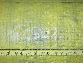
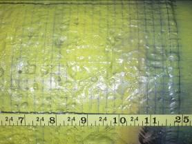
228 Figure 2-8. Defect P1-9 (P1-NC1) Pipeline Inspection Technologies Demonstration Report 27 Appendix D

229 S15 S13 S11 S9 S7 S5 S3 S1 Circumferential Distance (.25" increments) Axial Distance (.25" increments) Figure 2-8 (cont). Defect P1-9 (P1-NC1) Pipeline Inspection Technologies Demonstration Report 28 Appendix D

230 S S S8 S7 S6 S5 S4 S3 Circumferential Distance (.25" increments) S2 S Axial Distance (.25" increments) Figure 2-9. Defect P1-12 (Defect 6) Pipeline Inspection Technologies Demonstration Report 29 Appendix D

231 S S S7 S6 S5 S4 S3 S2 Circumferential Distance (.25" increments) S Axial Distance (.25" increments) Figure 2-1. Defect P1-13 (Defect 7) Pipeline Inspection Technologies Demonstration Report 3 Appendix D

232 S S S S2 S Axial Distance (.25" increments) S6 Circumferential Distance (.25" increments) Figure Defect P1-14 (Defect 8) Pipeline Inspection Technologies Demonstration Report 31 Appendix D

233 S S S8 S7 S6 S5 S4 S3 Circumferential Distance (.25" increments) S2 S Axial Distance (.25" increments) Figure Defect P1-18 (Defect 9) Pipeline Inspection Technologies Demonstration Report 32 Appendix D

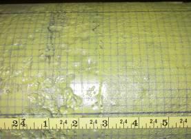
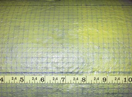
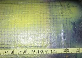
234 Figure Defect P1-21 (P1-NC2) Pipeline Inspection Technologies Demonstration Report 33 Appendix D

235 S17 S15 S13 S11 S9 S7 S5 S3 S1 Circumferential Distance (.25" increments) Axial Distance (.25" increments) Figure 2-13 (cont). Defect P1-21 (P1-NC2) Pipeline Inspection Technologies Demonstration Report 34 Appendix D

236 S S S8 S7 S6 S5 S4 S3 Circumferential Distance (.25" increments) S2 S Axial Distance (.25" increments) Figure Defect P1-22 (Defect 1) Pipeline Inspection Technologies Demonstration Report 35 Appendix D

237 S S S8 S7 S6 S5 S4 S3 S2 Circumferential Distance (.25" increments) S Axial Distance (.25" increments) Figure Defect P1-23 (Defect 11) Pipeline Inspection Technologies Demonstration Report 36 Appendix D

238 8 INCH PIPE SAMPLE 2 DOCUMENTATION Figure inch Pipe Sample 2 Defect Map Pipeline Inspection Technologies Demonstration Report 37 Appendix D

239 This page intentionally blank. Pipeline Inspection Technologies Demonstration Report 38 Appendix D

240 Pipe Sample 2 Simulated Corrosion Defect Photos S S S8 S7 S6 S5 S4 S3 Circumferential Distance (.25" increments) S2 S Axial Distance (.25" increments) Figure Defect P2-4 (Defect 1) Pipeline Inspection Technologies Demonstration Report 39 Appendix D

241 S S S S2 S Axial Distance (.25" increments) S6 Circumferential Distance (.25" increments) Figure Defect P2-6 (Defect 2) Pipeline Inspection Technologies Demonstration Report 4 Appendix D

242 S S S S2 S Axial Distance (.25" increments) S6 Circumferential Distance (.25" increments) Figure Defect P2-7 (Defect 3) Pipeline Inspection Technologies Demonstration Report 41 Appendix D

243 S S S8 S7 S6 S5 S4 S3 Circumferential Distance (.25" increments) S2 S Axial Distance (.25" increments) Figure 2-2. Defect P2-9 (Defect 4) Pipeline Inspection Technologies Demonstration Report 42 Appendix D

244 S S S8 S7 S6 S5 S4 S3 S2 Circumferential Distance (.25" increments) S Axial Distance (.25" increments) Figure Defect P2-1 (Defect 5) Pipeline Inspection Technologies Demonstration Report 43 Appendix D

245 S S S S2 S Axial Distance (.25" increments) S6 Circumferential Distance (.25" increments) Figure Calibration Defect P2-1 (Defect 6) Pipeline Inspection Technologies Demonstration Report 44 Appendix D

246 S S S8 S7 S6 S5 S4 S3 Circumferential Distance (.25" increments) S2 S Axial Distance (.25" increments) Figure Calibration Defect P2-2 (Defect 7) Pipeline Inspection Technologies Demonstration Report 45 Appendix D

247 S S S8 S7 S6 S5 S4 S3 Circumferential Distance (.25" increments) S2 S Axial Distance (.25" increments) Figure Defect P2-12 (Defect 8) Pipeline Inspection Technologies Demonstration Report 46 Appendix D

248 S S S S2 S Axial Distance (.25" increments) S6 Circumferential Distance (.25" increments) Figure Defect P2-14 (Defect 9) Pipeline Inspection Technologies Demonstration Report 47 Appendix D

249 S S S8 S7 S6 S5 S4 S3 Circumferential Distanced (.25" increments) S2 S Axial Distance (.25" increments) Figure Defect P2-17 (Defect 1) Pipeline Inspection Technologies Demonstration Report 48 Appendix D

250 S S S S2 S Axial Distance (.25" increments) S6 Circumferential Distance (.25" increments) Figure Defect P2-2 (Defect 11) Pipeline Inspection Technologies Demonstration Report 49 Appendix D

251 This page intentionally blank. Pipeline Inspection Technologies Demonstration Report 5 Appendix D

252 8 INCH PIPE SAMPLE 3 DOCUMENTATION Figure inch Pipe Sample 3 Defect Map Pipeline Inspection Technologies Demonstration Report 51 Appendix D

253 This page intentionally blank. Pipeline Inspection Technologies Demonstration Report 52 Appendix D

254 Pipe Sample 3 Simulated Corrosion Defect Photos S S S8 S7 S6 S5 S4 S3 Circumferential Distance (.25" increments) S2 S Axial Distance (.25" increments) Figure Calibration Defect P3-1 (Defect 1) Pipeline Inspection Technologies Demonstration Report 53 Appendix D

255 S S S8 S7 S6 S5 S4 S3 Circumferential Distance (.25" increments) S2 S Axial Distance (.25" increments) Figure 2-3. Defect P3-3 (Defect 2) Pipeline Inspection Technologies Demonstration Report 54 Appendix D

256 Figure Defect P3-4 (Defect 3) Pipeline Inspection Technologies Demonstration Report 55 Appendix D

257 S S S8 S7 S6 S5 S4 S3 Circumferential Distance (.25" increments) S2 S Axial Distance (.25" increments) Figure Defect P3-5 (Defect 4) Pipeline Inspection Technologies Demonstration Report 56 Appendix D

258 S S S8 S7 S6 S5 S4 S3 Circumferential Distance (.25" increments) S2 S Axial Distance (.25" increments) Figure Defect P3-7 (Defect 5) Pipeline Inspection Technologies Demonstration Report 57 Appendix D

259 Figure Defect P3-9 (Defect 6) Pipeline Inspection Technologies Demonstration Report 58 Appendix D

260 S Axial Distance (.25" increments) S S S S S2 Circumferential Distance (.25" increments) Figure Defect P3-1 (Defect 7) Pipeline Inspection Technologies Demonstration Report 59 Appendix D

261 S S S8 S7 S6 S5 S4 S3 Circumferential Distance (.25" increments) S2 S Axial Distance (.25" increments) Figure Defect P3-12 (Defect 8) Pipeline Inspection Technologies Demonstration Report 6 Appendix D

262 Figure Defect P3-14 (Defect 9) Pipeline Inspection Technologies Demonstration Report 61 Appendix D

263 S S S S2 S Axial Distance (.25" increments) S6 Circumferential Distance (.25" increments) Figure Defect P3-17 (Defect 1) Pipeline Inspection Technologies Demonstration Report 62 Appendix D

264 S S S S2 S Axial Distance (.25" increments) S6 Circumferential Distance (.25" increments) Figure Defect P3-18 (Defect 11) Pipeline Inspection Technologies Demonstration Report 63 Appendix D

265 Figure 2-4. Defect P3-19 (Defect 12) Pipeline Inspection Technologies Demonstration Report 64 Appendix D

266 S S S8 S7 S6 S5 S4 S3 Circumferential Distance (.25" increments) S2 S Axial Distance (.25" increments) Figure Defect P3-21 (Defect 13) Pipeline Inspection Technologies Demonstration Report 65 Appendix D

267 S S S8 S7 S6 S5 S4 S3 Circumferential Distance (.25" increments) S2 S Axial Distance (.25" increments) Figure Defect P3-23 (Defect 14) Pipeline Inspection Technologies Demonstration Report 66 Appendix D

268 SECTION 3. MECHANICAL DAMAGE INSPECTION TECHNOLOGY ASSESSMENT INTRODUCTION The current DOT PHMSA and DOE NETL developments for mechanical damage inspection technologies are not restrictive of pipe diameter. However, prior DOT PHMSA projects involved fabricating defect sets in 24 inch diameter pipe. Therefore when selecting the specimens and data for the mechanical damage defect set the use of the existing 24 inch diameter pipe samples was the most practical. An additional advantage of using the existing 24 inch defect sets is that they have already been inspected using MFL technology under a DOT contract. As such, magnetic flux leakage signals from these defects can be made available upon request. The technology developer examining mechanical damage anomalies has requested only smooth dents without gouges on the external surface. One pipe sample exists that meets the smooth dent requirement; however another defect set with dents fabricated with a track hoe are also included in the demonstration to assess the future potential of this technology. These defects have minimal gouging and therefore are the most appropriate for this demonstration. The following report sections discuss the demonstration plan for the mechanical damage inspection tools and provides an answer key (Table 3-1) for the data sheets given to the developer during the demonstration. Additional information and photographs are provided in Figures 3-1 through 3-4 describing how the dents were manufactured, the dent depths, dent lengths, and locations for all of the mechanical damage defects. 24-INCH MECHANICAL DAMAGE DEMONSTRATION PLAN The test plan for the 24-inch mechanical damage defect test configuration is as follows: 1. The technologies to be benchmarked include: 1.1. PNNL: Strain measurement tool 2. The pipe is 24-inch outside diameter 3. A guide rail was installed on the interior of each pipe to minimize rotation 4. The demonstration samples were comprised of two pipes: 4.1. Pipe 1 specifications are as follows: The length is approximately 28 feet; seam welded pipe The nominal wall thickness is.29 inches The pipe contained 17 mechanical damage defects created by direct impact with a 57, pound track hoe. Pipeline Inspection Technologies Demonstration Report 67 Appendix D

269 The defects were placed along 1 row with the guide rail located 18 away from the defects (or in a location determined by the sensor developer prior to the demonstration) The angular coverage area for each sensor technology should have been designed to cover +/- 6 inches on either side of the centerline (~6 angular coverage) All defects (except the calibration defects) were covered with a heavy material to prevent the sensor developer from viewing the defects. One defect near End A of the pipe sample remained uncovered for system check-out and calibration Pipe 2 specifications are as follows: The length is 4 feet of seam welded pipe The nominal wall thickness is.28 inches The pipe contained 1 smooth dents without gouges The defects were placed along 1 row with the guide rail located 18 away from the defects The angular coverage area for each sensor technology should have been designed to cover +/- 6 inches on either side of the centerline (~6 angular coverage) All defects (except the calibration defects) were covered with a heavy material to prevent the sensor developer from viewing the defects. Two defects near End A of the pipe sample remained uncovered for system check-out and calibration. Pipeline Inspection Technologies Demonstration Report 68 Appendix D

270 24 INCH MECHANICAL DAMAGE DEFECT ASSESSMENT DATA Table inch Mechanical Damage Inspection Technology Data Sheet Answer Key Pipeline Inspection Technologies Demonstration Report 69 Appendix D

271 Table 3-1 (cont). 24 inch Mechanical Damage Inspection Technology Data Sheet Answer Key Pipeline Inspection Technologies Demonstration Report 7 Appendix D

272 24 INCH MECHANICAL DAMAGE PIPE SAMPLE 1 DOCUMENTATION Pipe sample 1 was created from two sections of 24-inch diameter pipe with a wall thickness of.29-inches welded together to produce one longer length of pipe measuring approximately 28 feet in length. Pipe sample 1 was subsequently fitted with end caps containing nipples to allow water to pass into and out of the pipe to facilitate pipe pressurization during defect installation. The specifications for the individual pipe segments are provided in Table 1. For pipe sample 1, many magnetic, mechanical and chemical properties had been measured on a previous project; selected properties are included in Table 1. Table 3-2. Material and Mechanical Properties of Pipe Sample 1. Thin Wall Pipe Sample Property: PSF 24-6 PSF Diameter, in Wall Thickness, in Yield Stress, ksi Ultimate Stress, ksi Toughness, ft-lb Remnant Magnetism, G 12,1 9,9 Carbon, % Defect Installation Pipe Sample 1 contained three rows of mechanical damage defects, two rows were created with the dent and gouge machine and a third row was created with a 5-ton track hoe. Only the row of mechanical damage defects created by the track hoe was used for the benchmarking demonstration. However, to avoid possible mechanical and magnetic signal interaction, the other defect rows were spaced circumferentially by 12 increments and the defects were staggered axially by approximately a pipe diameter. During installation of each dent and gouge defect, the pressure in the pipe was held near 6 percent of the specified minimum yield stress (SMYS) of the weakest pipe. During installation of the track hoe defects, the pressure in the pipe was held near 15 percent of SMYS (2 psig). Prior experience has shown that even this relatively small amount of internal pressure adds significant stiffness to the pipe and causes defects to reround to nearly the same extent as defects made under fully pressurized conditions. Installing multiple defects in one pipe section necessitated moving the pipe axially and rotating it in the dent-and-gouge machine. The pressure in the pipe was reduced each time the pipe was moved to reduce the likelihood of damage growth or an accident. Therefore, defects installed early in the sequence were subjected to a number of pressure cycles of roughly 3 percent of the yield stress. Pipeline Inspection Technologies Demonstration Report 71 Appendix D

273 For defects made using the track hoe, a trench was excavated so that the pipe samples would fit securely within. The depth of the trench was slightly less than the pipe diameter so that the crown if the pipe was an inch or so above grade. The track hoe was able to straddle the trench so that the bucket could impact the crown of the pipe, parallel to the pipe direction, to produce the mechanical damage defects. The track hoe was also moved to the side of the trench so that defects could be produced that were transverse to the pipe direction. The location of mechanical damage defects are shown in Figure 3-1. Pipeline Inspection Technologies Demonstration Report 72 Appendix D

274 PIPE 24-6 PIPE APPROXIMATE SCALE 24 p6d3 p6d6 p6d9 p28d2 p28d5 p28d8 p28d11 p28d14 12 Side A p6d2 p6d5 p6d8 p28d1 p28d4 p28d7 p28d1 p28d13 Test Row p6dth1 p6dth2 p6dth3 p28dth4 p28dth1 p28dth *Could not easily identify weld Axial Distance (inches) Defect Length Dent Depth 2" 1% 4" 2% 6" 3% 8" 18" 2" 26" 27" 29" Figure inch Mechanical Damage Pipe Sample 1 Defect Map Pipeline Inspection Technologies Demonstration Report 73 Appendix D

275 This page intentionally blank. Pipeline Inspection Technologies Demonstration Report 74 Appendix D

276 Simulating Dents and Gouges with the Track Hoe The mechanical damage defect row used for the benchmarking demonstration was installed using a Kobelco Mark SK2 track hoe (see Figure 3-2). This particular track hoe is capable of producing a load of nearly 47, pounds. To the extent practical, the simulation was set-up to reflect actual conditions along the pipeline right-of-way. A trench slightly less than the pipe diameter was excavated so that the pipe samples would fit securely within. The pipe was placed within the trench and pressurized to approximately 2 psig. The track hoe was able to straddle the trench so that the bucket could impact the crown of the pipe, parallel to the pipe direction, to produce the mechanical damage defects. The track hoe was also moved to the side of the trench so that additional defects could be produced that were transverse to the pipe direction. Figure 3-2. Kobelco Mark SK2 Track Hoe. The track hoe bucket consisted of six teeth measuring approximately 6 inches in width and 1 inch in depth. Close-up photos of the track-hoe bucket and teeth are shown in Figure 3-3. Pipeline Inspection Technologies Demonstration Report 75 Appendix D

277 Figure 3-3. Close-Up of Bucket and Teeth from the Kobelco Mark SK2 Track Hoe. Additionally, the track hoe bucket was positioned in two different configurations during defect installation. The first configuration allowed the teeth of the bucket to directly impact the crown of the pipe. The second configuration allowed two teeth to straddle the crown of the pipe when impact was made. Various track hoe defect parameters for each pipe sample are provided in Table 3-3. For the track hoe defects, dent depth range refers to the maximum depth measured after defect installation and possible re-rounding. Table 3-3. Parameters for pipe sample 1 track hoe mechanical damage defects. Pipe 24-28, Internal Pressure of 2 psig Defect Description Tool Number of Strikes Strike Direction Bucket Tooth Position Dent Depth Range (inches) D13, D14, D15 (p28dth1) Parallel, direct TH 3 parallel direct D1, D11, D12, (p28dth2) Parallel, straddle TH 3 parallel straddle D7, D8, D9 (p28dth4) Transverse, direct TH 2 transverse direct Pipe 24-6, Internal Pressure of 2 psig Dent Length, in. Defect Description Tool Number of Strikes Strike Direction Bucket Tooth Position Dent Depth Range (inches) Calibration Defect (p6dth1) Parallel, direct TH 3 parallel direst D1, D2, D3 (p6dth2) Parallel, straddle TH 3 parallel straddle D4, D5 (p6dth3) Dent Length, in. Transverse, direct TH 1 transverse direct Pipeline Inspection Technologies Demonstration Report 76 Appendix D

278 Mechanical Damage Pipe Sample 1 Defect Photos Figure 3-4. Calibration Defect p6dth1 Pipeline Inspection Technologies Demonstration Report 77 Appendix D

279 Circumferential Extent (inches) Velocity = 5 mph Final Dent Depth =.35 inches Axial distance (inches) Depth =.1 inches Figure 3-5. Deformation Data for Calibration Defect p6dth Decoupled Circumferential Extent (inches) Axial distance (inches) Figure 3-6. MFL Signal for Calibration Defect p6dth1 Pipeline Inspection Technologies Demonstration Report 78 Appendix D

280 Figure 3-7. Defects D1, D2, and D3 (p6dth2) Pipeline Inspection Technologies Demonstration Report 79 Appendix D

281 Circumferential Extent (inches) Velocity = 5 mph Final Dent Depth =.24 inches Axial distance (inches) Depth =.1 inches Figure 3-8. Deformation Data for Defects D1, D2, and D3 (p6dth2) Decoupled Circumferential Extent (inches) Axial distance (inches) Figure 3-9. MFL Signal Data for Defects D1, D2, and D3 (p6dth2) Pipeline Inspection Technologies Demonstration Report 8 Appendix D

282 Figure 3-1. Defects D4 and D5 (p6dth3) Pipeline Inspection Technologies Demonstration Report 81 Appendix D

283 Circumferential Extent (inches) Velocity = 5 mph Final Dent Depth =.15 inches Axial distance (inches) Depth =.1 inches Figure Deformation Data for Defects D4 and D5 (p6dth3) Decoupled Circumferential Extent (inches) Axial distance (inches) Figure MFL Signal Data for Defects D4 and D5 (p6dth3) Pipeline Inspection Technologies Demonstration Report 82 Appendix D

284 Figure Defect D6 (Dent with Gouge; Not Part of Benchmarking) Circumferential Extent (inches) Velocity = 5 mph Final Dent Depth =.42 inches Axial distance (inches) Depth =.1 inches Figure Deformation Data for Defect D6 (Dent with Gouge; Not Part of Benchmarking) Pipeline Inspection Technologies Demonstration Report 83 Appendix D

285 Figure Defects D7, D8, D9 (p28dth4) Pipeline Inspection Technologies Demonstration Report 84 Appendix D

286 Circumferential Extent (inches) Velocity = 5 mph Final Dent Depth =.28 inches Axial distance (inches) Depth =.1 inches Figure Deformation Data for Defects D7, D8, D9 (p28dth4) Decoupled Circumferential Extent (inches) Axial distance (inches) Figure MFL Signal Data for Defects D7, D8, D9 (p28dth4) Pipeline Inspection Technologies Demonstration Report 85 Appendix D

287 Figure Defects D1, D11, D12 (p28dth1) Pipeline Inspection Technologies Demonstration Report 86 Appendix D

288 Circumferential Extent (inches) Velocity = 5 mph Final Dent Depth =.48 inches Axial distance (inches) Depth =.1 inches Figure Deformation Data for Defects D1, D11, D12 (p28dth1) Decoupled Circumferential Extent (inches) Axial distance (inches) Figure 3-2. MFL Signal Data for Defects D1, D11, D12 (p28dth1) Pipeline Inspection Technologies Demonstration Report 87 Appendix D

289 Figure Defects D13, D14, D15 (p28dth2) Pipeline Inspection Technologies Demonstration Report 88 Appendix D

290 Circumferential Extent (inches) Velocity = 5 mph Final Dent Depth =.48 inches Axial distance (inches) Depth =.1 inches Figure Deformation Data for Defects D13, D14, D15 (p28dth2) Decoupled Circumferential Extent (inches) Axial distance (inches) Figure MFL Signal Data for Defects D13, D14, D15 (p28dth2) Pipeline Inspection Technologies Demonstration Report 89 Appendix D

291 24 INCH MECHANICAL DAMAGE PIPE SAMPLE 2 DOCUMENTATION Plain dents represent the other fundamental part of mechanical damage where the natural cylindrical shape of the pipe is distorted. The dents in mechanical damage Pipe Sample 2 were made without gouging, so that the response of inspection systems to dents could be examined without compensation for the geometry changes, such as removed metal, and stresses caused by the gouge process. This section describes the methods and equipment used to fabricate the dent-only defects. The description is followed by detailed information of each dent and photographs. Data Collection Procedure The procedure for the incremental denting and data collection was a follows: 1. Pressurize the 24-inch diameter,.28-inch wall pipe to 6 psi, or about 4 percent of specified minimum yield stress (SMYS) of the this X6 pipe 2. Acquire baseline MFL data prior to denting, but with denting apparatus positioned (about one percent of maximum dent load was applied to hold reaction frame in place) 3. Apply hydraulic pressure to indent the pipe in increments of.5 percent of the pipe diameter (.12 inches) 4. Acquire axial MFL data with the indenter in place to keep the dent from rebounding 5. Repeat steps 3 and 4 until a maximum dent depth of 2 percent is a attained 6. Allow the dent to rebound.5 percent of the pipe diameter, matching the indenting steps 7. Acquire MFL with the indenter in place to keep the dent from further rebounding 8. Repeat steps 6 and 7 until the denting load is zero indicating the dent has finished rebounding. The equipment for the experiments is described in two subsections that follow. The first subsection describes a denting apparatus with a hydraulic actuator and reaction frame. The second subsection describes the flanged pipe sample with components that enable a MFL inspection pig to be launched, pulled back and forth during the dent forming process, and accessed between inspections. Denting Apparatus The apparatus used to dent the pipe in a controlled manner is illustrated in Figure The operation of the equipment is simple. A hydraulic cylinder is extended between a pipe sample and a stiff reaction frame. The reaction frame was a previously used I-beam with the web reinforced to minimize deformation during the application of the denting load. A 1-inch thick plate was welded to the beam for support of the hydraulic cylinder. The weakest component of Pipeline Inspection Technologies Demonstration Report 9 Appendix D

292 the apparatus is the pipe wall that is in contact with the indenter. As the hydraulic load increases, the pipe deforms. To determine the amount of deformation, two measurements are made by linear cable extension transducers, commonly referred to as string pots. The first string pot measures the extension of indenting tool. The second string pot measures the separation between the pipe and the reaction frame, which increases during the formation of the dents since the many components elastically bend and extend. The depth of the dent is established by the difference between the I-beam with reinforced web Hydraulic Ram 1, psi Rating Pipe displacement (string pot) Tool displacement (string pot) Indenting tool 6-inch shaft.281 wall X6 Pipe Reaction Chain Figure Denting apparatus configuration including reaction frame, hydraulic actuator displacement transducers, pipe sample and load reaction chains. two measurements. The dents were formed by slowly increasing the pressure until depth was attained. The denting process took between 2 and 3 minutes. Since the pipe was pressured to 6 psi, the pump was located 15 feet from the actuator for safety concerns. Pipeline Inspection Technologies Demonstration Report 91 Appendix D

293 Pressurized Pull Rig To evaluate leakage signals from dents as they form and rebound under internal pressure, a method was established to acquire flux leakage at multiple pressures repeatedly at multiple magnetization levels. The experimental configuration, shown in Figure 3-25, is essentially a pressurized version of a pull rig. The components include: A new pipe sample configured with flanges on either end. This was a.281-inch wall thickness, 24-inch diameter, 6 ksi yield pipe. A pig launching barrel for insertion of the circumferential magnetizer and data recorder. This was a.5-inch wall thickness, 24-inch diameter, 6 ksi yield pipe from existing pipe inventory. A hinged pressure door for insertion and access to the magnetizer and data recording equipment. Two rods for pulling the magnetizer and data recording equipment in either direction. Rod seals to hold pressure as the equipment is pulled. These seals are commonly used in oil well pumping operations. A pressure relief valve to prevent over pressurizing. This was required to adequately address safety concerns. After each increment of dent depth, the MFL inspection pig was pulled from one end of the pipe sample and back to the return position. During the pulling of the pig, leakage in the rod seals would cause a drop in internal pressure in the pipe. Lubricating the rod with light oil reduced wear on the seal, minimizing pressure losses to less than 5 psi or 1 percent on each pull. Three indenters were used to dent the pipe. Each indenter was made from a non-ferromagnetic 3 series stainless steel. Each shaft was 6 inches long to keep the ferromagnetic hydraulic actuator sufficiently away from the pipe to minimize interference with the flux leakage inspection equipment. Figure 3-26 shows a spherical indenter made from 1.5-inch diameter rod, photographed during the denting process. Figure 3-27 shows the two longer indenters. The radius of the rounded indenter matches the spherical indenter radius of.75 inches. The sharp indenter is rounded to a radius of.125 inches to provide a more concentrated load, but avoid piercing. The length of the long rounded indenter and the long sharp indenter is 4.5 inches. The shape changes were chosen to facilitate comparison of results. For the spherical and long rounded indenter, the radius is the same but the contact shape is changed from a sphere to a cylinder. For the two longer indenters, the length was the same, but the contact shape is changed from gradual to abrupt. Pipeline Inspection Technologies Demonstration Report 92 Appendix D

294 Pressure Relief 1 Dent Locations Spaced 3 feet Apart Launch Barrel Launch Door Flange 6 PSI Nitrogen Supply 12 V Battery Pulling Rods High Pressure Rod Seals Figure Pressurized pull rig for acquisition of MFL data during incremental denting and rebounding. Pipeline Inspection Technologies Demonstration Report 93 Appendix D

295 Figure The spherical indenter, made from a non-ferromagnetic material, photographed while holding a 2 percent dent. Note the connections for the two linear cable extension transducers. 1.5 inch 4.5 inches Long Cylindrical Tool Long Wedge Tool Figure Diagram of two other indenters used in incremental denting and data recording experiments. Pipeline Inspection Technologies Demonstration Report 94 Appendix D

296 Plain Dent Defects A total of 1 defects were made with three indenters at two magnetization levels, as shown in Table 3-4. Table 3-4. Incremental dent defects Defect # Calibration Dent R1 Calibration Dent R2 R3 R4 R5 R6 R7 R8 R9 R1 Indenter Spherical Long Cylindrical Spherical Long Wedge Long Cylindrical Spherical Long Cylindrical Long Wedge Long Cylindrical Long Wedge Table 3-5 shows the final dimensions of the dents used for evaluation. Since dents do not have distinct start and end points, measurements can be subjective; the length measurements for Defect R5 are illustrated in Figure The total length and width were defined by a.25- inch departure from the nominal shape of the pipe. The reround lengths were defined by a more abrupt departure from the nominal shape of the pipe. The surface length is the length that the indenter was in hard contact with the pipe. Because of irregularities of the pipe shape itself, the accuracy of the length and width measurements is ±.5 inch and the accuracy of the depth measurement is ±.1 inch. The defect map for pipe sample 2 is presented in Figure Table 3-5. Dimensions of the dents used for the primary comparisons of the high and low magnetization signals. Dent Dimension (inches) Total Reround Surface % W.T. # Indenter Signal Length Length Length Width Depth Depth R1 Spherical High % R2 Long Cylindrical High % R3 Spherical High % R4 Long Wedge High % R5 Long Cylindrical High % R6 Spherical Low % R7 Long Cylindrical Low % R8 Long Wedge Low % R9 Long Cylindrical Low % R1 Long Wedge Low % Pipeline Inspection Technologies Demonstration Report 95 Appendix D

297 Defect 5 Long Cylindrical High Mag One inch Height Distorted 4x One inch 4.5 inches Surface length 8.5 inches reround length 12 inches Total length Figure Dent length measurements for the long cylindrical indenter. Pipeline Inspection Technologies Demonstration Report 96 Appendix D

298 Figure inch Mechanical Damage Pipe Sample 2 Defect Map Pipeline Inspection Technologies Demonstration Report 97 Appendix D

299 This page intentionally blank. Pipeline Inspection Technologies Demonstration Report 98 Appendix D

300 Mechanical Damage Pipe Sample 2 Defect Photos Figure 3-3. Calibration Defect R1 Pipeline Inspection Technologies Demonstration Report 99 Appendix D

301 Figure Calibration Defect R2 Pipeline Inspection Technologies Demonstration Report 1 Appendix D

302 Figure Defect R3 Pipeline Inspection Technologies Demonstration Report 11 Appendix D

303 Figure Defect R4 Pipeline Inspection Technologies Demonstration Report 12 Appendix D

304 Figure Defect R5 Pipeline Inspection Technologies Demonstration Report 13 Appendix D

305 Figure Defect R6 Pipeline Inspection Technologies Demonstration Report 14 Appendix D

306 Figure Defect R7 Pipeline Inspection Technologies Demonstration Report 15 Appendix D

307 Figure Defect R8 Pipeline Inspection Technologies Demonstration Report 16 Appendix D

308 Figure Defect R9 Pipeline Inspection Technologies Demonstration Report 17 Appendix D

309 Figure Defect R1 Pipeline Inspection Technologies Demonstration Report 18 Appendix D

310 Figure 3-4. Blank R11 Pipeline Inspection Technologies Demonstration Report 19 Appendix D

311 SECTION 4. SCC INSPECTION TECHNOLOGY ASSESSMENT INTRODUCTION The focus of the SCC assessment projects is to develop ultrasonic technologies that can operate in natural gas pipelines. Crack detection technology for liquid pipelines is already commercially available. However, transmitting ultrasonic energy into and out of the pipe without the use of a liquid coupling agent is necessary for the practical inspection of natural gas transmission pipelines. Stress corrosion cracks are more commonly found in larger diameter pipelines because typical operating pressures produce sufficient stress in the pipe wall to initiate and grow cracks. From an inspection technology viewpoint, the sensors have a relatively large footprint. A typical sensor footprint, without engineering to make them smaller, is on the order of 1 cm (4 inches) per quarter. SCC pipe samples also appear to be more readily available in larger diameter pipes. Therefore, for these practical and implementation reasons, the capability of SCC detection technology is initially focused on pipe diameters greater than 24 inches. The PSF has available a large number of SCC defects in 26-inch diameter pipe acquired through donations from PRCI member companies. One of the technology developers has already used pipe samples at the PSF and therefore these samples are not included as part of the demonstration. In addition, the external coating on the pipe itself is a significant variable and therefore only pipe without coating was made available for the benchmarking demonstration. The report sections below discuss the demonstration plan for the SCC inspection tool and provides an answer key (Table 4-1) for the data sheets filled out by the SCC inspection tool developer during the demonstration. Additional information and photographs are provided in Figures 4-1 through 4-8 which show the magnetic particle maps and the locations and lengths of the natural SCC defects. 26-INCH STRESS CORROSION CRACK DEMONSTRATION PLAN The test plan for the 26-inch stress corrosion crack test configuration is as follows: 1. The technology(s) to be benchmarked include: 1.1. ORNL: Strain measurement tool 2. Total length of the pipe sample will be 26 feet 3. The pipe will be 26-inch outside diameter 4. The test sample is comprised of one pipe: Pipeline Inspection Technologies Demonstration Report 11 Appendix D

312 4.1. The length is approximately 26 feet of seam welded pipe 4.2. The nominal wall thickness is.281 inches 4.3. The pipe contained 7 stress corrosion crack colonies for examination 4.4. The pipe sample had multiple defect locations requiring three rows for data collection The pipe did not have any external coating All defects (except the calibration defects) were covered with a heavy material to prevent the sensor developer from viewing the defects. A separate SCC pipe sample measuring 38-feet in length was available for system check-out and calibration. Pipeline Inspection Technologies Demonstration Report 111 Appendix D

313 This page intentionally blank. Pipeline Inspection Technologies Demonstration Report 112 Appendix D

314 26 INCH SCC DEFECT ASSESSMENT INFORMATION Table inch SCC Inspection Technology Data Sheet Answer Key Pipeline Inspection Technologies Demonstration Report 113 Appendix D

315 Table 4-1 (cont). 26 inch SCC Inspection Technology Data Sheet Answer Key Pipeline Inspection Technologies Demonstration Report 114 Appendix D

316 Table 4-1 (cont). 26 inch SCC Inspection Technology Data Sheet Answer Key Pipeline Inspection Technologies Demonstration Report 115 Appendix D

317 26 INCH SCC PIPE SAMPLE 893 DOCUMENTATION Pipe Sample No. 893 Drawing #1 of 2 Ind.# Cracks Max Size Cracked Area Old Distances EOP Distance L.W. New Distances EOP to start of box inches inches inches inches Inches 1 multi ¼ 2 x 1 ¾ A 9 18 ¼ A Not Available 2 multi ¼ 2 x 2 A A Not Available 3 multi 1 ½ 11 x 7 A A Not Available 4 multi ¼ 5 ¼ x 1 ¼ A 28 ¾ 33 B 233 ¼ 5 multi ¼ 4 x 1 ½ A 216 ¾ 32 B 225 ¼ 6 multi ½ 3 x 2 ½ B B 21 ¾ 7 multi ¼` 4 ¼ x 3 ¾ B 193 ½ 16 ½ B 189 ¼ 8 multi ¼ 2 ¾ x 2 ½ B B 29 ¼ 9 multi ¼ 3 ½ x 3 ½ B 145 ¾ 19 ¼ B 141 ½ 1 multi ¼ 3 ½ x B multi ¾ 2 x 2 A A -- Not Available A portion of pipe specimen 893 was cut and used for another project. The cut portion is no longer available for use. The new distances from the edge of the pipe are presented in the table. Figure 4-1. SCC Pipe 893 Data Pipeline Inspection Technologies Demonstration Report 116 Appendix D

318 Pipe Sample No. 893 Drawing #2 of 2 Ind.# Cracks Max Size Cracked Area Old Distances EOP Distance L.W. New Distances EOP to start of box inches inches inches inches Inches 11 multi ¾ 2 x 2 A 11 see dwg #1 33 A Not Available 12 ¾ ¾ A 49 ½ 38 A Not Available 13 ¼ ¼ A 15 ½ 3 A Not Available A A Not Available 15 ½ ½ A B 37 ½ 16 multi ¾ 17 x 1 ¾ A 26 8 B 224 ¼ A B 218 ¼ 18 ½ ½ B B 213 ¾ B 213 ½ 27 ½ B 27 ½ B 94 4 B 88 Figure 4-1 (cont). SCC Pipe 893 Data Pipeline Inspection Technologies Demonstration Report 117 Appendix D

319 Figure 4-2. Diagram of SCC Pipe 893 Pipeline Inspection Technologies Demonstration Report 118 Appendix D

320 Data Sheet Code # Indication # Max Size Cracks Area Cracked Distance to Start of Crack Area (from End of Pipe Side B) Distance L/W (from weld to start of crack area) Line # SCC1 Blank 3 *** *** *** *** Line 1 SCC2 4 & 5 ¼ 5 ¼ x 1 ¼ and 4 x 1 ½ and 32 Line 1 SCC3 8 ¼ 2 ¾ x 2 ½ Line 1 SCC4 Blank 2 *** *** *** *** Line 1 SCC5 Blank 1 *** *** *** *** Line 1 SCC6 Blank 5 *** *** *** *** Line 2 SCC7 Blank 4 *** *** *** *** Line 2 SCC8 6 ½ 3 x 2 ½ Line 2 SCC9 7 ¼ 4 ¼ x 3 ¾ Line 2 SCC1 9 ¼ 3 ½ x 3 ½ Line 2 SCC11 16 ¾ 17 x 1¾ Line 3 SCC12 Blank 8 *** *** *** *** Line 3 SCC13 Blank 7 *** *** *** *** Line 3 SCC14 Blank 6 Table 4-2. SCC Pipe 893 Data *** *** *** *** Line 3 Pipeline Inspection Technologies Demonstration Report 119 Appendix D

321 Pipe 193 SCC Defect Photos Figure 4-3. Defect SCC 2 (4 & 5) Pipeline Inspection Technologies Demonstration Report 12 Appendix D

322 Figure 4-4. SCC 3 (8) Figure 4-5. Defect SCC 8 (6) Pipeline Inspection Technologies Demonstration Report 121 Appendix D

323 Figure 4-6. Defect SCC 9 (7) Figure 4-7. Defect SCC 1 (9) Pipeline Inspection Technologies Demonstration Report 122 Appendix D

324 Figure 4-8. Defect SCC 11 (16) Pipeline Inspection Technologies Demonstration Report 123 Appendix D

325 SECTION 5. PLASTIC PIPE INSPECTION TECHNOLOGY ASSESSMENT INTRODUCTION One new sensor technology was added in this Phase II Benchmarking Demonstration. This technology inspects plastic pipe for small volumetric anomalies with a detection threshold of approximately.15 cubic inches. The measurement technology is localized and therefore anomalies in close proximity and pipe end effects do not influence its detection capabilities. Battelle procured a medium density polyethylene pipe sample (yellow in color) for the benchmarking demonstration. The pipe sample has an inside diameter of approximately 5.5- inches and wall thickness of.5 inch. Cylindrical hole and saw cut defects were manufactured along one row of the pipe sample to assess the capabilities of the sensor technology. The report sections below discuss the demonstration plan for the plastic pipe inspection tool and provides an answer key (Table 5-1) for the data sheets filled out by the inspection tool developer during the demonstration. Additional information and photographs are provided in Figures 5-1 through 5-13 which show the locations and size of the plastic pipe defects. This information was used as the guide to assess the performance of the sensor technology developer. 6 INCH PLASTIC PIPE DEMONSTRATION PLAN The demonstration plan for the 6-inch plastic pipe test configuration is as follows: 1. The technologies benchmarked included: a. DOE NETL plastic pipe sensor 2. The pipe is 6.5-inch outside diameter 3. The pipe wall thickness is.5 inch making the inside diameter approximately 5.5 inches. The pipe had some ovality and a slight twist. 4. The demonstration sample was comprised of one medium density (yellow) polyethylene pipe: 3.1. A 13 foot long 6" Polyethylene Pipe positioned horizontally was used as the test sample. The sample was supported from the bottom and only at the ends A single row of defects was located directly above the center line (plus or minus 1/4 inch). Defects were placed 6 to 7 inches apart and one foot from the end, allowing 2 defect locations. Pipeline Inspection Technologies Demonstration Report 124 Appendix D

326 3.3. Eight locations did not have a defect. Defects were covered with a heavy material to prevent sensor developers from viewing the defects. One defect near End A remained uncovered for system check-out and calibration Typical defects included small cylindrical holes and saw cuts. The volume of these defects ranged from.15 to.5 cubic inches. All defects were on the outside surface of the pipe sample. Pipeline Inspection Technologies Demonstration Report 125 Appendix D

327 6 INCH PLASTIC PIPE ASSESSMENT INFORMATION Table inch Plastic Pipe Inspection Technology Data Sheet Answer Key Pipeline Inspection Technologies Demonstration Report 126 Appendix D

328 6 INCH PLASTIC PIPE SAMPLE DOCUMENTATION Figure inch Plastic Pipe Sample Defect Map Pipeline Inspection Technologies Demonstration Report 127 Appendix D

329 Plastic Pipe Sample Defect Photos Figure 5-2. Calibration Defect C1 Figure 5-3. Defect D1 (D1) Pipeline Inspection Technologies Demonstration Report 128 Appendix D

330 Figure 5-4. Defect D4 (D2) Figure 5-5. Defect D5 (D3) Pipeline Inspection Technologies Demonstration Report 129 Appendix D

331 Figure 5-6. Defect D7 (D4) Figure 5-7. Defect D1 (D5) Pipeline Inspection Technologies Demonstration Report 13 Appendix D

332 Figure 5-8. Defect D12 (D6) Figure 5-9. Defect D13 (D7) Pipeline Inspection Technologies Demonstration Report 131 Appendix D

333 Figure 5-1. Defect D14 (D8) Figure Defect D15 (D9) Pipeline Inspection Technologies Demonstration Report 132 Appendix D