OSIRIS USERS MANUAL WARNING. OH- Suppressing Infra-Red Imaging Spectrograph

Transcription

1 OSIRIS OH- Suppressing Infra-Red Imaging Spectrograph Not Your Grandma s Spectrograph USERS MANUAL WARNING Entering Deep Water If In Doubt, Don t Go Out James Larkin, Matthew Barczys, Mike McElwain, Marshall Perrin, Jason Weiss, Shelley Wright UCLA Infrared Laboratory Version 2.2 April 1, 2008

2 Intentionally Blank -2-

3 A Subset of the OSIRIS team with the dewar on the Keck II Nasmyth Deck. OSIRIS and CARA members at OSIRIS first light (Keck II remote OPS). -3-

4 Table of Contents 1 OSIRIS Overview OSIRIS Capabilities Basic Optical Layout Lenslet Geometry Filters and Fields of View Dispersions and Resolutions Lenslet Fill Factor Concentricity of the Four Plate Scales Optical Error Budget Throughputs Sensitivities Imager Observing with Adaptive Optics Observing procedures User Interface Field Acquisition Spectroscopic Calibration Telluric Standards Wavelength Calibrations Data Reduction System Major Changes to the Pipeline for Version Changes to the Pipeline for Version Changes to the Pipeline for Version Installing the Pipeline at Your Home Institution ODRFGUI: The OSIRIS Data Reduction File GUI Working Directly with Data Reduction XML Files (DRFs) Reducing a Normal Observation Output Filename Construction Reducing Multiple Darks or Skies into a Super File Mosaicking Multiple Science Exposures Module Descriptions Adjust Channel Levels Assemble Data Cube Calibrate Wavelength Clean Cosmic Rays Combine Frames Correct Dispersion Determine Mosaic Positions Divide Blackbody Divide by Star Spectrum Extract Spectra Extract Star Glitch Identification Mosaic Frames

5 Remove Crosstalk Remove Hydrogen Lines Rename Files Save DataSet Information Scaled Sky Subtraction Subtract Frame Appendix A Detector Performance A.1 Characterization Data A.2 Memory Charge A.3 Fixed Pattern Noise and Artifacts A.4 Spectrograph Detector and Detector Controller A.5 Optimization of Detector Operating Temperature A.5.1 Temperature Dependence of QE A.5.2 Temperature Dependence of the Reset Anomaly A.5.3 Optimum Operating Temperature A.6 Spectrograph Detector Crosstalk Appendix B Filter Curves Appendix C Atmospheric Transmission Appendix D Atmospheric Dispersion D.1 Instrumental Chromatic Dispersion Appendix E FITS header keywords Appendix F History of Instrument Changes / Which matrices to use in reductions Appendix G When all else fails Play Cowboy

6 1 OSIRIS Overview OSIRIS is an integral field spectrograph (IFS) designed to work with the Keck Adaptive Optics System. It uses an array of tiny lenses to sample a rectangular patch of the focal plane and produces spectra at up to 3000 locations simultaneously. There is also an internal diffraction limited camera with a 20 field of view. Both the camera and spectrograph can operate at wavelengths between 1 and 2.4 microns. The center of the imaging camera s field is about 20 offset from the center of the spectrograph field and both can be used simultaneously with the same or different filters. The spectrograph has plate scales of 0.020, 0.035, and arcsec per lenslet. The spectral resolution averages 3800 in the three finest plate scales, but is closer to 3000 in the arcsec plate scale. In the broadband mode each spectrum contains a full broad band (z, J, H or K) and a total of 16x64 (actually 1019) spectra are taken. In the narrowband mode, a typical spectrum contains 1/4 th of a broad band and an individual exposure contains between 16x64 to 48x64 spectra depending on the exact filter selected. The imager has a single fixed plate scale of arcsec per pixel and suffers from some vignetting in the corners of the array. A great deal of thought has gone into trying to make OSIRIS easy to use. For the spectrograph, the only user selectable items are the plate scale, the filter and the exposure time. The imager only has a filter and an exposure time setting. A great deal of complexity, however, is allowed in the observing sequences and the slaving of the imager to the spectrograph. All setup and control aspects of the instrument are managed by a few GUIs. There is also a data reduction system that includes a real-time reduction of raw frames into cubes for display and basic analysis. In this real-time mode, it takes about 1 minute for a preliminary data cube to appear in the quicklook display package. The reduction system also includes a growing set of final reduction steps including correction of telluric absorption and mosaicking of multiple cubes. That being said, infrared spectroscopy is a fairly complex astrophysical technique, and when combined with a laser adaptive optics system, and the complexity of over 3000 independent and overlapping spectra, OSIRIS is not recommended for the faint of heart. In terms of observing planning, much of the complication actually comes from the AO nature of the instrument. As an imaging spectrograph, much of the dithering and exposure settings are quite similar to a traditional infrared camera or spectrograph. Since the infrared background is bright and complicated, it s important to obtain sky frames for subtraction, but in some cases where your object is small, you can build a sky by dithering on-chip (in this case on-lenslet but it s identical). Similarly, telluric standard stars are needed in most cases to remove atmospheric transmission variations as a function of airmass and wavelength. Like NIRSPEC or other IR spectrographs, we ve found that stars near spectral types A0 work well, although others sometimes use solar analogs. Much of this is discussed in detail within this manual, but we thought it was important to give you an initial sense of how the instrument works. Basically pick a filter and platescale then dither on source and on sky. The pipeline will handle much of the rest. For the latest information on OSIRIS, please always refer to the website which will have links to the most recent versions of software and documentation. It also has links to an OSIRIS wiki page for users. -6-

7 2 OSIRIS Capabilities 2.1 Basic Optical Layout A schematic of the OSIRIS IFS optical configuration is shown in Figure 2-1. The IF spectrograph optical configuration consists of three coupled systems: a re-imager, an image sampler, and a spectrograph. The image sampler is a 2-dimensional array of small lenses or lenslets located at a re-imaged focal plane of the Keck II AO system. At the focus of each lenslet a much smaller pupil image is formed that contains all of the light from its portion of the field. This lenslet array serves to spatially sample the input image. The pupil images are well separated and serve to define the entrance aperture of the spectrograph section. The dispersion axis of the spectrographic is rotated slightly compared to the lenslet orientations so that the dispersed spectra from each spatial location are interleaved across the spectrograph detector. The spatial scale of the instrument is determined by re-imaging optics in front of the lenslet array. The re-imaging optics also provides most of the baffling within the instrument including a cold pupil stop. Spectrograph Cold stop Lenslet array Adjustable mask Collimator optics (TMA) Keck II AO focus Fixed grating Filters Re-imager collimator (singlet) R.I. Camera (singlet) Re-imaged focal plane Pupil plane Camera optics (TMA) Re-imaging optics Image sampler Detector Figure 2-1: OSIRIS Spectrograph Optical Configuration -7-

8 Fold Mirror & Lenslet Array Grating Reimaging Cameras Filter s Spectrograph Collimator Mirrors (TMA) OSIRIS Optical Layout AO Focus Reimaging Collimators Hawaii-2 Detector Fold Mirror Spectrograph Camera Mirrors (TMA) Figure 2-2: Rendering of the real optics within the spectrograph leg of the instrument. Note that the lenslet array is the smallest component. The reimaging optics are fully refractive to reduce wavefront error, while the spectrograph optics are all off-axis mirrors to eliminate ghosts. Each lenslet in a given row is the source for a spectrum that is nominally separated by 2 pixels vertically from the spectrum of the adjacent lenslet in the same row. Each spectrum is also offset or staggered horizontally. The stagger results from the slight rotation of the lenslet array relative to the detector. The horizontal stagger should be 32 pixels, but anamorphism introduced by the TMA in the horizontal direction causes the offset to be reduced to ~29 pixels. This makes better use of the detector real estate in the horizontal direction by allowing longer spectra to fit onto the detector. -8-

9 2.2 Lenslet Geometry The lenslet array is rotated by 3.6 degrees relative to the dispersion axis of the grating, which itself is aligned to rows of the detector. This allows the spectra from neighboring lenslets to miss each other on the detector and to be successfully interleaved. A side-effect of this is that rows and columns of the lenslet move diagonally across the detector at an angle of 3.6 degrees. To keep the spectra roughly centered on the array, we stagger the lenslets every 16 th row (tan(3.6)=1/16). So in the end, 51 columns and 66 rows of lenslets are at least partially illuminated. Figure 2-3 shows the geometry of illuminated lenslets. We refer to the bottom left lenslet as [1,1]. Note that it is not illuminated. Broad Band ~16x64 Narrow Band ~48x64 Figure 2-3: 51 columns and 66 rows of lenslets are at least partially illuminated. The pattern above shows in white the lenslets that are illuminated in the narrow band mode, and in blue for the broad band mode. Note that in many narrow band filters, not all of the white lenslets are available either due to order overlap, or that the spectra fall off the detector. See Section 2.3 for exact sizes. Also note that 15 lenslets marked in red are lost off the top of the detector and are not available. -9-

10 2.3 Filters and Fields of View OSIRIS provides four spatial scales to choose from (0.020, 0.035, and 100 arcsec per lenslet). There are also subtle differences in the spatial scales in terms of the effective pupil size matched to each scale. This leads to differences in terms of the sensitivities and backgrounds of the four scales. In a little more detail, the scales are achieved by swapping in matched pairs of lenses that magnify the images onto the lenslet array. As Figure 2-4 shows, they all must have the same physical length of 700 mm and there are constraints about the physical size and location of the lens and filter mechanisms. In particular, the magnification is basically the ratio of the focal length of the camera lens to the collimator lens. For the 20 mas scale, this requires us to go from an F/15 beam to an F/257 beam or a magnification of So its collimator lens has a very short focal length of only 20 mm, so its cold pupil is roughly 20 mm behind the lens. The collimator for the coarsest scale is closer to 100 mm, so its pupil is roughly 200 mm from the input AO focus. In the end, only each of the three fine scales (20, 35 and 50 mas) have a cold pupil stop mounted with them, while the coarse scale (100 mas) has a fixed cold stop permanently mounted in the optical path. This has the unfortunate effect that it must be oversized to allow through all of the other beams and allows through considerable excess thermal background. In order to lower thermal background at longer wavelengths, in March 2008 the OSIRIS team smaller pupil sizes designed smaller 100 mas pupils to be used with duplicate K filters. There are four filter holders and four new pupils that were attached individually for each duplicate K filter (Kbb, Kn3, Kn4, Kn5). The pupil sizes for each of the scales and the new effective 9 meter inscribed pupil for the 100mas scale is illustrated in Figure arcsec scale: This is the only scale that has proper sampling across the AO PSFs for wavelengths longer than 1.5 microns. So it is optimized for image quality and has a slightly oversized pupil that is circumscribed around the m outer edges of the Keck telescope. Because of this, it has an elevated thermal background (K=11.2 mag/sq arcsec). At wavelengths below 2 microns it is primarily read noise limited so the coarser scales have better raw sensitivity & arcsec scales: These two scales are optimized for maximum sensitivity at thermal wavelengths (K~11.8 mag/sq arcsec). They both have circular pupils equivalent to a 10- meter telescope so they slightly clip the edges of the Keck primary. But since they have coarse sampling, the PSF is not significantly affected arcsec scale: Originally this was only included to help with target acquisition, but many users have expressed interest in using it for faint targets. There are several important caveats with using this scale. First, as the scales get coarser, the geometric pupils formed by the lenslet array grow. Since OSIRIS is a pupil spectrograph, the final spectral resolution and cross contamination between spectra are directly dependent on the size of the pupils. Diffraction helps to keep the 20, 35 and 50 mas pupils close to the same size as each other, and the spectral resolution of ~3800 refers to these scales. The 100 mas scale is coarse enough that even with perfect optics, it would produce a 2x2 pixel blur on -10-

11 the detector. With aberrations and diffraction this becomes 2.5 to 3 pixels and results in a reduced spectral resolution of less than 3400, and additional contamination from neighboring spectra. The pupil is oversized and allows through a great deal of excess infrared background (K=10.6 mag/sq ). In order to alleviate this excess background at the coarsest scale, we have installed duplicate K-band filters with their own smaller 100mas pupils (9-m effective). Lenslet Location Camera Lenses Filter Locations Cold Pupils Collimators AO Focus Figure 2-4: Optical paths of the four sets of reimaging -11- optics. In reality, the lenses are mounted in 4/1/2008 turrets in wheel mechanisms, but here we show them side by side for comparison. UCLA Infrared Laboratory

12 35 & 50 mas pupils 100mas Kband Pupils 10 m m 20 mas pupil 100 mas Pupil Figure 2-5: Scale drawing of the pupils for each of the four plate scales. Note that the 100 mas pupil is significantly oversized to allow the other scales optical path not to be vignetted. To lower the thermal background at longer wavelengths there is a smaller 100mas pupil installed just for the Kband filters (magenta). -12-

13 There are a total of 23 filters available within the spectrograph. Originally there were 4 broadband filters and 18 narrowband filters, but since installation of the duplicate K-band filters with smaller 100mas pupils in March 2008, there are now 5 broadband filters and 18 narrowband filters (we used an open position for adding one of the duplicate filters. The combination of filters and scales results in 88 discreet modes. For each of the broadbands, the spectra fit completely on the detector in a single exposure for the central 16x64 lenslets. But since the grating does not move in OSIRIS, the narrow band filters shift on the detector depending on where they fall within the broadband spectrum. So, for example, the Kn1 spectra from the central 16x64 spectra fall at the short wavelength end of the location where the Kbb spectra fall which is at the edge of the detector. So lenslets on one side of the central 16x64 are actually more centered, while those on the other side fall off the detector. This leads to only the central narrow band filters falling onto the detector for the full 48x64 lenslets. Filters are either extreme (Kn1 or Kn5 for example) have some spectra off the detector and so have more limited fields of view. In addition, the Z and J bandpasses are working at 6 th and 5 th diffraction orders, respectively. So the neighboring orders fall fairly close on the detector, and order overlap makes the left-most and right-most lenslets in the narrowbands unusable. Order overlap also limits the wavelength coverage of the broad band Z filter. The long wavelength half-power point of the Zbb filter lands in the 7 th order on top of microns in the 6 th order. So typical wavelength extractions are limited to wavelengths greater than microns. Table 2-1 gives the wavelength range of each filter (50% transmission points are quoted), along with the # of simultaneous spectra that are obtained in each exposure, the approximate geometry of the spectra on the sky, and the fields of view for each of the 4 plate scales. In most cases, if a narrow band filter does not cover 48x64 lenslets, then it is also displaced slightly left or right on the sky. The planning gui will show the true coverage of each filter compared to the OSPEC pointing origin. But all filters include the central 16x64 lenslets. Appendix Appendix B gives the filter transmission curves. Take note that the filters named Kcb, Kc3, Kc4, and Kc5 in the OSIRIS planning GUI (OOPGUI) are just duplicate Kbb, Kn3, Kn4, and Kn5 filters with the smaller 100mas pupil. -13-

14 Table 2-1: OSIRIS Spectrograph Filters, Scales and Fields of View Shortest Longest Number of Number of Approx. Wavelength Wavelength Spectral Complete Lenslet FOV for FOV for FOV for FOV for Channels Filter Extracted(nm) Extracted(nm) Spectra Geometry Zbb 999 * 1176 * x x x x x 6.4 Jbb * x x x x x 6.4 Hbb x x x x x 6.4 Kbb* x x x x x 6.4 Zn x x x x x 6.4 Jn x x x x x 6.4 Jn x x x x x 6.4 Jn x x x x x 6.4 Jn x x x x x 6.4 Hn x x x x x 6.4 Hn x x x x x 6.4 Hn x x x x x 6.4 Hn x x x x x 6.4 Hn x x x x x 6.4 Kn x x x x x 6.4 Kn x x x x x 6.4 Kn3* x x x x x 6.4 Kn4* x x x x x 6.4 Kn x x x x x 6.4 * Limited by overlap from other orders. * The Kcb, Kc3, Kc4, and Kc5 filter names are identical to these respective filters. -14-

15 Table 2-2 lists the original filter lists of the spectrograph before the March 2008 servicing which swamped out the Zn2, Zn3, and Zn5 filters for the new duplicate K-band filters with smaller 100mas pupils. The first four rows of Table 2-2 describe the broad band filters for the spectrograph. The table lists the original OSIRIS filter specifications (first two columns titled Design Specs ), the actual central wavelength (CWL) and bandwidth (BW) as measured in OSIRIS in the next two columns, and the remaining columns to the right list the filter parameters for the actual filters as measured by the filter manufacturer. Table 2-2: OSIRIS Spectrograph Filter Parameters Design Specs Measured in OSIRIS Test Data Supplied by Filter Manufacturer Filter Name CWL (nm) BW (nm) CWL (nm) BW (nm) CWL (nm) BW (nm) Avg T Rise Fall Slope RMS wfe P-V wfe Power (%) Slope (%) (%) (waves) (waves) (waves) Zbb Jbb Not avail. Hbb Not avail. Kbb Zn Zn Zn Zn Jn Jn Jn Jn Hn Hn Hn Hn Hn Kn Kn Kn Kn Kn All of the measured values for BW and CWL are based on the 50% power points. For the Zbb and Jbb filters, the useful ranges are actually set by order overlap and are given in Table 2-1. For the manufacturer s test data slope, is determined based on the 80% and 5% relative transmission points. The wavefront error (wfe in the table), peak to valley wavefront error (P-V wfe in the table) and the optical power are given in wavelengths of light (waves) at nm. -15-

16 2.4 Dispersions and Resolutions OSIRIS can take up to 3072 spectra simultaneously. Due to variations in the incident and diffracted angles with the grating, and with spot quality at the detector, the spectral resolution has significant variation between lenslets and at different wavelengths. The dispersions on the detector are actually fairly constant and have median values given in Table 2-3. Table 2-3: Linear Dispersion Median Dispersion per pixel in raw data (μm/pix) Resampled Dispersion in Reduced Cubes (μm/pix) Band (order) Z (6 th ) J (5 th ) H (4 th ) K (3 rd ) Over the central 16x64 lenslets which include the full broad band, the median spectral resolution in the scale is 3900, and the average resolution is The difference comes from the fact that the long wavelength end of spectra tend to have fairly constant resolutions just above 4000, while the short wavelengths within each order fall to about Figure 2-6 shows the spectral resolution achieved at a wavelength of microns. Notice the bright region near lenslet [38,12] where the FWHM is typically less than 2 pixels leading to a spectral resolution above Towards the lower right, the FWHM begins to increase and the spectral resolution bottoms out around The graph in Figure 2-7 shows the more complex variation of spectral resolution as a function of position and wavelength. -16-

17 Figure 2-6: This is the effective spectral resolution achieved as a function of lenslet position at a wavelength of microns. It includes the linear dispersion and the measured FWHM of an arcline at this wavelength. Notice that spectral resolutions are highest near lenslet [38, 12] and are lowest near lenslet [22,50]. For numeric values, use the graph shown in Figure

18 Best Lenslet Median Lenslet Worst Lenslet Figure 2-7: The spectral resolution depends on lenslet number and wavelength. This graph shows the resolution as a function of wavelength in the 3 rd order (K band) over the primary 16x64 lenslet positions (median resolution at each wavelength), the highest resolution region (lenslets near [22, 50]) and the lowest wavelength region (lenslets near [38,12]). Other bands are simple scalings of this relationship, i.e. the J band is observed in 5 th order, so the same resolution occurs at 3/5ths of the wavelengths shown in the graph. This is for the scale, although the and scales are similar. -18-

19 2.5 Lenslet Fill Factor According the test report supplied by the manufacturer there is a 2-3 micron rounding between the nominally square lenslets. This results in a fill factor of approximately 95%. Additionally, the test report supplied by the manufacturer indicates that the transmittance of the lenslet array is between 95 % and 97%. The peak transmittance is at 1.2 µm. 2.6 Concentricity of the Four Plate Scales An important consideration is how well aligned are the four spectrograph plate scales. If you acquire an object in the center of one scale, then you can NOT simply select another scale and remain centered on your object. Table 2-4 below gives the relative offset between the field centers of the four scales. It is important, however, to remember that if an object appears centered in the scale, this represents 5 pixels within the scale, so a small shift in addition to the table offsets may occur. The table assumes that an object has been centered in the scale and then calculates by how much it will shift in reduced data cubes if another scale is selected and the object is not moved. X-offset refers to the short (16 or 48 lenslet) axis, while the Y-offset refers to the long (64 lenslet) axis. Table 2-4: Relative Offsets between the Four plate Scales. Scale Xoffset (arcsec) Yoffset (arcsec) To compensate for these small offsets, the Telescope GUI (OTGUI) can be used to offset an object from the center (or specified pixel) in one plate scale to the center (or specified pixel) in another plate scale, or even to the imager. -19-

20 2.7 Optical Error Budget In Table 2-5 below, we give the estimated RMS wavefront error of each optical element in the spectrograph up to but not including the lenslet array and all elements of the imager. These are the elements that affect the Strehl ratios. In the case of mirrors, the wavefront error is assumed to be twice the surface error. For the window, lenses and filters the wavefront error is assumed to be equal to (n-1) times the sum in quadrature of the two surface errors. In all cases, the measurements were made over an area equal to or larger than the illuminated region. In some cases, more than one component was fabricated, and the component currently in the instrument is identified in the table. Table 2-5:Optical Error Budget Component Design RMS WFE (nm) Fabricated RMS WFE (nm) Window (1) (n=1.458) 4 3 Window (2) (will be installed at summit) Window (3) (in dewar) Splitter Mirror Spectrograph (1) 13 3 (in dewar) Splitter Mirror Spectrograph (2) Splitter Mirror Imager (1) 13 8 (in dewar) Splitter Mirror Imager (2) 13 9 Lenslet Fold Mirror (1) Lenslet Fold Mirror (2) (in dewar) Spectrograph Fold Mirror (1) 13 6 (in dewar) Spectrograph Fold Mirror (3) 13 8 Spectrograph Fold Mirror (4) 13 4 Imager Fold Mirror (1) 13 8 Imager Fold Mirror (2) 13 3 (in dewar) F/257 Collimator (n=1.474) F/257 Camera (n=1.474) 17 9 Imager M Imager M Imager M Imager M Filters (min:mean:max) 12 2:5.5:10 Imager Surface Total (alignment errors ignored) Imager design WFE 25 Imager alignment tolerances 30 Spectrograph Total (0.02 scale) Imager Total (design+align+surface) <45 The scale is very insensitive to alignment issues, since there are only two powered optics and these are simple biconvex lenses. Tipping or tilting them to first order causes image motion. Sufficient tilt to contribute to the wavefront error budget would shift the images off the small lenslet field. The same is true of the coarser scales, but they are also much more tolerant to wavefront error due to sampling issues. So the spectrograph tip/tilt and decenter requirements -20-

21 from the OSIRIS Mechanical Design Note (OMDN) Section 5 must be satisfied in order to achieve the observed image quality. The imager has three powered surfaces, but these are also spherical which are relatively insensitive to alignment errors. To reach the 30 nm of WFE allowed for imager internal alignment, the detector would be focused 7 mm from nominal which would be easily seen in our mounting, and would shift the plate scale away from our measured value of by more than 5% which is not observed in either measurement method. This level of alignment error also tends to make the plate scales in each direction different which is not observed. 2.8 Throughputs In this section we summarize the vendor data on individual component efficiency, along with the estimate of the grating efficiency as derived from the relative efficiency of the spectrograph and imager. For simple elements such as the gold mirror or BaF 2 lenses, we use the coating reflectances or transmittances supplied by the coating vendor. Notice that the measured efficiencies in the H and K bands are comparable to each other but about 30% lower than expected. We have somewhat arbitrarily assigned the majority of this to the grating. In the J- band, however, the efficiency falls dramatically to only 2.7%. We do not know the source of this efficiency loss, and we believe it is unfair to assign the full extent to OSIRIS. We note that NIRC2 appears to have at least a factor of 2 loss of efficiency from the K to the J bands. Table 2-6 lists the component efficiencies as presented at the PDR and as-built. Table 2-6: Predicted and As-built Efficiencies OPTICAL ELEMENT Efficiency predicted at PDR As-built measured efficiency (H and K bands) Window 97% 97% Fold Mirrors NA 96% Collimator Lens 92% 96% Filters 75% 70-93% (avg. = 80.0%) Camera Lens 92% 96% Lenslet Array (AR Coated, 2 surfaces) 96% 95% TMA Collimator (4 mirrors, 99%; includes first 92% (assumes some dirt) 96% fold) Grating (varies with wavelength) 70% peak 42% avg Camera Optics (4 mirrors, 99%; includes fold) 96% 92% Total Optical Throughput 38% 23% Detector Quantum Efficiency 65% 81% OSIRIS Total Throughput 25% 19% Telescope Transmission 80% 80% AO Transmission 65% 65% Atmosphere 90% 90% TOTAL THROUGHPUT 12% 8.8% -21-

22 2.9 Sensitivities OSIRIS object sensitivities are a little more complicated to calculate than with a normal instrument. The OSIRIS throughput varies through each band due to the atmospheric transmission, blaze function of the grating and filter functions. With an imager all of these factors can often be combined into a single zero point for each filter. But for a spectrograph, there is in essence a different zero point for every spectral channel. In addition, the spectra all have slight variations in efficiency primarily due to detector effects, and different angles and footprints on the grating. There is also the added complexity of adaptive optics imaging and the unpredictable Strehl ratio that you will achieve on your science target. Nevertheless, OSIRIS offers substantially better capability for true spectral photometry compared to a traditional slit spectrograph due to its integral field nature. So in principle the PSF can be fully characterized, and in most cases point sources are fully covered by the fields of view. For sensitivity calculations each spectrum is spread over more than one detector pixel, so the extraction algorithm sweeps up more than one pixel s worth of noise. The amount of read noise per spectral channel therefore depends weakly on plate scale and wavelength. The best demonstrated read noise per pixel using the up-the-ramp sampling method is 4.8 electrons (this actually also includes a dark current and detector glow component). With the new grating installed in June, 2005, arclines are more elongated perpendicular to the dispersion axis than at the time of preship. This leads to more read noise per spectral channel than with the original grating, although several other factors including throughput improved dramatically. A typical read noise component for extracted spectra is about 10 electrons in the up-the-ramp mode. In Table 2-7 below, we give the zero points for the OSIRIS spectrograph expressed in extracted DN/sec. In these units, the zero points are defined in the standard way: Mag = -2.5 log(flux in DN/sec) + Mag(zero point) Table 2-7: Spectrograph Zero Points Band J H K Spectrograph Zero Points (if flux is in DN/sec) 23.5 mag 24.3 mag 23.7 mag To convert to electrons, assume a detector gain of 0.23 DN per electron. To calculate rough sensitivities for a continuum source, estimate the flux per lenslet element for your target assuming a reasonable Strehl ratio (see the AO page for expected Strehls with the Laser or NGS targets). You can then use the zero points to determine the number of data numbers per lenslet that will be generated per second. Multiply this by your exposure time, and divide by 1700 (roughly the number of spectral channels). This will give you the number of DN per spectral channel, and compare that to 4 data numbers to get a rough signal to noise for an individual exposure for each lenslet. -22-

23 2.10 Imager The imager uses a Hawaii-1 detector from Rockwell Scientific and has a 1024x1024 pixel format. The plate scale is arcsec per pixel for a total field of view of 20.4 arcsec. It is sensitive from 1 to 2.5 microns. The minimum exposure time is 2 seconds and times are limited to integer seconds. The imager holds virtually an identical set of filters as the spectrograph, but due to space within the filter wheels, does not have Zn2, Zn4, Zn5 or Jn4 filters (see Table 1). The imager field is offset from the spectrograph so that both can be used simultaneously without the need for beam splitters or dichroics. There were several motivations for the imager, including field acquisition and imaging science. But the primary purpose of the imager, and the reason for simultaneous viewing, is to track changes in the point spread function (PSF). As with all adaptive optics systems, the image quality is continuously changing and is difficult to predict purely from the wavefront sensor data. Also, for many science cases, the spectrograph target cannot be used to measure its own PSF. So the imager s goal is to measure the PSF from off-axis stars to at least allow for monitoring of the variation of conditions with time. Making use of the PSF stars to predict the PSF at the science target is still a major goal of many adaptive optics groups and is not a fully solved problem. The imager and spectrograph are in a fixed orientation compared to each other, but they can be dithered on the sky, and the pattern can be rotated to arbitrary angles Imager Field 20.4 x20.4 Spectrograph Fields: Up to 4.8 x6.4 at approximately 45 degrees Horizontal plane of Keck II AO bench and OSIRIS internal optical bench Figure 2-7: Relative locations of the imager and spectrograph focal planes. For the imager, in most cases you will be background limited. So the noise is dominated by the sky background. As you can see, the background in the K band is significantly elevated over NIRC or NIRSPEC. This is primarily due to the increased background from the AO system, but it is also due to the optical design of the imager. It is based on the SHARC camera and is close to an Offner optical design. This leads to excellent image quality with simple optics, but the pupil is poorly formed and not directly on an available optical surface. So the cold pupil is oversized and allows through additional background. Due to this background, the H band is definitely the deepest imaging filter. But care must be taken for some sources, since all of the OSIRIS filters -23-

24 were designed around the blaze functions of the OSIRIS spectrometer. These filters are typically wider than traditional infrared filters and photometric corrections will be necessary for objects with extreme colors, or that are line dominated. Filter curves are given in Appendix C. Imager Zero Point and Background Zero Point Background Band mag (in DN) mag / sq arcsec. J 27.8 mag 16.2 H 28.1 mag 14.6 K 27.6 mag

25 3 Observing with Adaptive Optics Coordination between OSIRIS and the AO system is largely handled automatically, but the user needs to be aware of certain limitations. Pre-observing planning on each science target is needed. The relative position of the guide star to the science fields is not completely arbitrary due to the position of the AO system s optical axis with respect to the OSIRIS optical axis, and the range of travel of the AO Field Steering Mirrors. A planning tool to help determine the ranges of position angles that are possible for a given guide star/science object geometry is available at

26 4 Observing procedures 4.1 User Interface Observational Planning GUI The OSIRIS planning GUI (OOPGUI) is your main interface for making observations. It allows users to plan observational sequences on one field with both the spectrograph and imager. Observers are able to change the filter, scale, coadds, itime, and dither patterns. The Dataset and Object fields are used for header information. The LGS mode is used to determine whether the laser should be dithered with your dither pattern or if it should remain fixed on-axis. IMPORTANT: The Kcb, Kc3, Kc4, and Kc5 filters are designed to only be used with 100 mas scale. Users must select both the combination of Kc filter and the 100mas scale! -26-

27 In practice, we ve found that the fixed position is optimal. The dither pattern is determined within the Object Frames and Sky Frames fields. For instance, in the above example the observer has set up three exposures on the science target (frames 1,2,3) with a raster scan and two additional sky frames. The first sky frame (frame 4) is offset from the science target by 5 west and 5 north, and the second sky frame (frame 5) is offset relative to the first sky frame by 0.35 west. There are multiple dither pattern options to select from: Stare (no dither), Box 4, Box 5, Box 9, Raster Scan, Statistical, and User Defined. The Show Position List button opens another window (bottom left image) that lists all the frames with their x and y offsets of the dither positions. It shows sky frames and the sequence of the observations. You may change the order of the frames by selecting one of the frames and using the Up, Down, Top, and Bottom buttons, as demonstrated on the bottom right image, which now has the last sky frame (number 5) being taken at the beginning of the observation sequence. -27-

28 If you are taking imager frames as well, the dither pattern chosen will reflect both the spectrograph and the imager since they are fixed relative to each other (bottom left image). The imager has several options: Disable (SPEC only), Independent (Imager only), Maximum Repeats, Maximum Itime, and Filter Sets. The Maximum Repeats, Maximum Itime, and Filter Sets are all based on the total integration time of the SPEC frames. The Maximum Repeats does the maximum number of imager frames with a user specified imager itime. The Maximum Itime calculates the maximum itime the imager can do given a user specified number of repeats. The Filter Sets is the most flexible option and allows users to use more than one filter and to directly specify the itime, coadds, number of repeats for each filter. When you select the Filter Sets option and click on the Filter field another window opens (bottom right image) for the user to interact with each of the values. Altering any of these fields in the GUI does not directly communicate with the instrument or the telescope. Once the observation sequence is prepared click the Send to Queue button, which adds the Dataset script (called a Data Definition File or.ddf) to a directory queue which the execution client GUI uses to build a list of observations. It s important to note that the position angle (PA) input does not alter the PA of the instrument once the DDF is executed. Altering the PA needs to be performed in the Telescope GUI (OTGUI). The correct PA is critical to make the proper dithers when moving in sky coordinates. Users may also save their observation planning sequence (.DDF) for later use or for planning before they arrive at the telescope. The GUI can be downloaded to your home computer before your run so you can practice laying out your observations. It s available at the OSIRIS website:

29 Execution Client GUI The execution client is the GUI that manages your observing sequences and implements them with the hardware control software. Once you have planned your observations in the OOPGUI (described above) you will Send to QUEUE, which sends your planned observations to this GUI. Once you are ready to start your observations you click Start Next Dataset which then commands the instrument and telescope. You only run this GUI at the telescope and it s easiest to learn at the telescope. It only has a few options including removing sequences that you don t want to execute, and starting sequences in the queue. For convenience, it also has the ability of starting spectrometer or imager frames using the current exposure settings. If you decide during an observational sequence that you wish to terminate or stop the sequence CAUTION should be taken. In most cases users should always use the Abort After Current Spec, which allows the current integration to finish exposing (with no effects to the detector) and then terminates the rest of the observing sequence. The Abort All Immediately should be used ONLY in dire need. This will stop the observation sequence in mid integration and resets all the voltages of the detector controller, which causes detector thermal problems which may take up to 15 minutes to clear. Flushing the detector will become necessary before resuming observations. Please see the Telescope GUI (OTGUI) section for instructions on how to flush the detector. -29-

30 Status GUI The Status GUI presents the current positions of all the motor mechanisms of OSIRIS spectrograph and imager. When the mechanisms are physically moving in the instrument the wheeled images will move on the GUI. The integration of a current file in the spectrograph and imager are updated as the exposure is being taken for monitoring. -30-

31 Telescope GUI The OSIRIS telescope GUI is used to input and send all commands to the telescope. The white box is used for logging which commands where issued. The GUI has a set of tabbed headings which bring down different control options. The Cover folder is blank and hides the other folders so observers do not accidentally click and move the telescope. The GUI will automatically switch to this cover when not in use. The Offset folder allows users to center the spectrograph between different modes (filter and scale), and offset to the imager. It also allows users to offset in RA and DEC in arcsec or detector pixels (it will use the current scale of the instrument so check the status GUI). The Rotate folder changes the position angle of OSIRIS. The Adaptive Optics folder allows input wait4ao ON or OFF. The script "wait4ao determines whether you want the observations to wait for the AO loops (DM and TT) to close before taking an exposure. You can either select wait4ao which includes both the DM and TT or wait4dm or wait4tt ON or OFF, The OSIRIS folder allows you to flush the spectrograph and imager detector. It takes a number of short integrations to clear the detector. This should only be done if persistence is seen in the detector from a bright star or if there are detector artifacts after issuing the command, Abort All Immediately. -31-

32 On-line Reduction GUI At the telescope, the OSIRIS pipeline is always waiting for a new raw file to be written so the little oompa loompas can generate a reduced cube for observational viewing and acquisition needs. The on-line reduction GUI (OORGUI) allows observers to select the calibration files for the Subtract Frame and Extract Spectra modules. In most cases, there should be no need to edit the calibration file for the Extract Spectra module since the GUI will automatically select the most recent rectification matrix based on the observed filter and scale. The Subtract Frame module can either use a specified FITS file, the first file generated from a dataset, or the second file generated from a dataset. For example, if dataset number 32 had two frames where frame 1 was a star and frame 2 was sky, then you would select Next Raw Frame. If instead dataset number 32 had two frames where frame 1 was sky and frame 2 was the star, then you would select Previous Raw Frame. If the Skip module is selected for a blue highlighted module, then that module will not be used in the pipeline and will be greyed out (i.e., Remove Crosstalk module in the image below) in the GUI. Please refer to Section 5 for a detailed description of the Data Reduction Pipeline. -32-

33 Quicklook2 OSIRIS spectrograph frames are 3D FITS files that require sophisticated image visualization tools. The OSIRIS team presents an IDL based software package called Quicklook2 to display and analyze your OSIRIS data cubes. Quicklook2 is the OSIRIS image analysis software used at Keck while observing, but we also encouraged using Quicklook2 for post-observing analysis of 2D/3D FITS. This software handles simple image analysis functions such as horizontal and vertical cut plotting, surface and contour plotting, color stretching, photometry analysis, image arithmetic, and zooms. At the same time, Quicklook2 is equipped with enhanced image analysis procedures for image rotations, wavelength information, and line fitting. The main image analysis GUI in Quicklook2 is shown below for reference. For a complete description of Quicklook2 functionality and operating procedures, please see the Quicklook2 Users Manual, which is available for download at the url This manual also has detailed instructions on installing Quicklook2 onto local machines. This software package supports the UNIX, Linux, Mac OS, and Windows operating systems. -33-

34 4.2 Field Acquisition As an imaging spectrograph, it is easier to acquire targets with OSIRIS than with traditional slit spectrometers, but the AO system and some details of the instrument can make field acquisition non-trivial. Most observations require a separate tip/tilt (TT) star for AO correction. Since acquisition of science targets is often performed as a blind offset from this star, it is imperative that the coordinates of the science target and the TT star are consistent with each other. Given the small field of view of the OSIRIS spectrograph, small errors in position can leave the science target just off the field. Given the faint nature of many science targets, it is easy to waste time integrating at the region adjacent to your science target. Please pay attention to issues such as mismatches in coordinates between catalogs, which can be particularly prevalent between older and newer stellar catalogs, such as HD and HST. Also, proper motions of stars can be significant between your observing date and the observing epoch in a catalog. Remember that for OSIRIS being off by just 1 arcsec can make a big difference! In general, it is very important to use the Keck s AO planning tools before your run to determine the position angles and offsets from your tip-tilt stars. For large offsets from the star, you may need to use different PAs so that both spectrograph and imager frames can be taken without defaulting the AO field steering mirrors (FSM). However, if your science is purely with the spectrograph, then in most cases you do NOT need to take acquisition frames with the imager first. The procedure below is the most common type of acquisition: acquiring a science target directly to the spectrograph. Important to the acquisition process is putting targets accurately at the center of the spectrograph field of view, which is called the OSPEC pointing origin by the telescope software. The OSPEC pointing origin is the center of reduced cubes in the scale for all broadband filters and the narrowband filters Zn3, Jn3, Hn3 and Kn3. For the other plate scales and filters, the center of the field is slightly offset (see Section 2.6 and the OTGUI of Section 4.1). During the afternoon, your support astronomer will typically use the fiber source in the AO system to refine this pointing reference. The acquisition procedure to place a science target on OSPEC is as follows: (1) Ask the OA to slew the telescope to the primary TT star of your desired science target (2) During the slew, adjust the position angle to the desired value using Rotate tab on the OTGUI (See Section 4.1). (3) When the rotation is complete, locate the TT star on the guider display using a finding chart. Ask the OA to acquire the TT reference star to the OSPEC pointing origin by giving the pixel coordinates of the TT star on the guider (often this will be obvious and the OA will immediate acquire the star). The OA should acquire to the OSPEC pointing origin using the Adjust Pointing button on xguide. The TT star should now be centered on OSPEC. -34-

35 (4) If you are planning to take science frames in the scale in a filter for which OSPEC is the center (see above), skip to the next step. Otherwise, you must perform an offset to put the TT star in the center of your working scale and filter. On the Offset tab of the OTGUI, perform a move from the center of any OSPECcentered filter in mode to the center of the scale and filter you plan to use for your science. (5) Once you ve moved the star to your particular center location, take an on-source and off-source (or sky) pair of images. Using the OOPGUI, define a dataset with a stare exposure with no offset as the object frame, and a stare exposure with an offset of ~5 arcsec as the sky frame. When the second exposure is complete, the online DRP will produce a data cube containing the star. The online DRP reduction should take about a minute. If the star is in the field but does not appear in the center, use the OTGUI to move it to the center position by specifying which pixel the star is currently located on and move it to the field center. Make sure the filter and scale are both set to your working scale and wavelength. If the star does not appear in the field at all, make sure that the AO system is still locked on the star, and that you are at the OSPEC pointing origin (ask your OA). If everything seems right but you don t see the star, it may be off the field. Try switching to a narrow band filter in the scale to get the maximum field of view (4.8 x6.4 ). If the star is faint, try increasing the exposure time (although 60 seconds should be sufficient to see any TT star). If desired, you can take a pair of exposures to verify the centering of the TT star. However, this is not normally needed, and it will cost you time for the exposures and reduction. This is normally not necessary, but one option would be to start the exposures and go on to the next step while you wait for the pipeline to finish. (6) Once the TT star is centered, ask the OA to Mark Base (this is particularly important for the Mosaic Frames module, see Section 5.7). This will set the current offset values to zero and make the telescope RA and DEC keywords match the sky. Then, ask the OA to Offset to science target, which will place your science target on the OSPEC pointing origin. In LGS-AO operations, the OA will acquire using LGS- AO-Acq on OSPEC. (7) Begin science observations. -35-

36 4.3 Spectroscopic Calibration Telluric Standards The atmosphere in the infrared has significant transmission variation both with wavelength and with time. In order to properly reduce a spectrum, this transmission must be estimated at an elevation and atmospheric condition close to your science target. We recommend using an A0 star within 0.1 airmasses of your science exposure. Stars with magnitudes between 7 and 9 work well and typical exposure times are 20 seconds. If you spend roughly an hour on a given target field, we often select a telluric star at about the same declination but 30 minutes later in RA from the science target. This will place the star at about the average location in the sky that the science exposures were taken. The pipeline modules Extract Star, Remove Hydrogen Lines and Divide by Blackbody work to produce a 1D spectrum of a star taken for telluric correction. To work properly, the star must be at least 4 pixels from the field edges and must have no significant spectral features besides hydrogen absorption lines. This typically means using stars near spectral type A Wavelength Calibrations The OSIRIS wavelength solution is calculated in vacuum units. The IAU standard for conversion from air to vacuum wavelengths is given in Morton (1991, ApJS, 77, 119) and is reproduced here: λvac λ AIR = λvac λvac The wavelength solution is extremely stable and the user does not need any additional observations. A single global wavelength calibration comes with the pipeline. Before pipeline version 2.0, the wavelength solution was solely based on arc line positions produced from a set of calibration lamps. These don t fill the pupil uniformly so the line centers appear to have a slight wavelength shift (usually about 0.1 pixels, 0.3 nm in K band or less, but in some regions as much as 0.5 pixels). To achieve a better wavelength solution, Tuan Do was able to use the cross correlation of OH lines in the Kn3 filter and determine an average shift for each lenslet between the arc line positions and sky line locations (which should uniformly fill the pupil like an astrophysical object). This offset has now been implemented in version 2.0 of the pipeline and significantly improves the differential line shifts from one lenslet to another. In what is likely to be one of the worst cases, Tuan used the new pipeline and looked at the cross correlation shifts in the Hn5 filter and found that the rms shifts between lenslets is now 0.04 pixels (0.08 Angstroms in H-band) with minimum and maximum deviations at the extreme corners of the array of 0.13 pixels (0.26 Angstroms). A further wavelength refinement is anticipated shortly, but if additional accuracy is needed, then we recommend reducing one of your frames with a dark frame for subtraction. This will leave OH-lines in the spectrum which can then be fit for their spectral position as a function of lenslet. The OH-lines then serve as a local spectral reference close to your science wavelengths. At the long end of K-band, this does not work since the last OH-line is around 2.2 microns. It is likely that some of the weak atmospheric absorption features at the end of K band might provide a suitable reference, but we have not tested this process. -36-

37 5 Data Reduction System Reducing data with OSIRIS is actually quite similar to reducing other infrared images and spectra. Since the infrared background is bright and complicated, it is very important to have sky frames for subtraction. Like images, these can sometimes be made by dithering on chip (in this case on lenslet ). Each lenslet s spectrum is also basically the same as any other spectrograph s spectrum. But there can be over 3000 of them and each has a slightly different path through the optics, so each spectrum has slightly different spectral dispersion, resolution and PSF quality. The most unique aspect of the instrument is that the 3000 spectra all partially overlap on the detector and do so at staggered wavelengths. A very custom routine is necessary for uniquely assigning flux from detector pixels back into lenslet spectra. We call this the Spectral Extraction process and it is quite similar to Lucy-Richardson deconvolution. Maps of the point spread function of each lenslet are made at all wavelengths (called Rectification Matrices or Extraction Matrices ). These maps are referenced in the extraction process. These matrices appear to be extremely stable (<0.1 pixels) over an indefinite period of time and the user does not need to take new matrices on their own. It is important, however, that you retrieve a set of matrices that match your data. There is a different map for each combination of filter and plate scale. Due to the unique nature of OSIRIS data and of its calibration steps, the OSIRIS team has developed a pipeline designed to reduce all of the calibration data, and to reduce scientific data to the level where an astronomer can begin custom analysis. The pipeline is an IDL program that accepts commands only from XML files, which we will refer to as Data Reduction Files (DRFs). Historically, these files must be created by hand and then placed into the agreed upon queue directory (see below). Now the DRFGUI generates XML directly and can automatically submit them into the queue directory. When you unpack the pipeline, one of the directories created will be: drs/drf_queue Any file placed in this directory with a numeric prefix and an extension of.waiting will be interpreted as a pending DRF file for processing. The pipeline will attempt to read the file and parse the instructions. It will also change the extension to.working while it is processing. If the reduction completes successfully, then the extension will be changed to.done. If the reduction fails, then the extension will be changed to.failed. If multiple.waiting files exist, then the pipeline will reduce them according to their numerical prefixes. In run_odrp, the o stands for OSIRIS. There are multiple pipelines in the sense that the pipeline will treat data of different types in different ways. There is actually a calibration pipeline, a stellar pipeline, an online pipeline and a final pipeline. But this is somewhat artificial and all pipelines can be executed by the single pipeline process simply by specifying the type of reduction you d like in the first line of the DRF. The reason for the distinction is that each "pipeline" can in principle use different module code attached to the same command. For example, if you use the Extract Spectra command in your DRF file, it will do something different in the online pipeline compared to the final pipeline. In this particular case, it s just the number of iterations that are performed, which ensures the online version is fast. The final -37-

38 pipeline will complete more iterations, which will result in cleaner spectra. A configuration file (RPBconfig.xml) is part of the pipeline distribution and specifies which modules are allowed for each pipeline and which.pro file to use for a particular command. In the case of spectral extraction, a single program is called, but it forks to different algorithms based on which pipeline was specified. In principle, when you are taking data and have the pipeline running in the background, it can perform any type of reduction. The OORGUI is what actually senses new frames and "drops" DRF files into the queue with the ORP specification. During a long exposure, you could just as easily use the final reduction GUI (DRFGUI), or the osirisdropdrf command to put a calibration or final xml file into the queue. General Suggestions If you see strange artifacts in the reduced cubes, especially roughly rectangular groups of lenslets that are offset in intensity from the main group of lenslets, then it may be useful to first process files without the Extract Spectra and Assemble Data Cube routines. This will produce images that are 2048x2048 pixels in size and are basically cleaned versions of the raw detector signals. Look for blocks of pixels jumping up and down by a few data numbers (channel offsets), or streaks running vertically through the lower left or upper right quadrants (crosstalk). The basic routines work in most cases, but they can be fooled by bright objects on channel boundaries. Try skipping Adjust Channel Levels, and Remove Crosstalk and see if the raw signals look improved. When the 2D data looks smooth, then process to completion with Extract Spectra and Assemble Data Cube. Also note that Glitch Identification does not replace the pixels in the 2D data. Instead, it flags the pixels as bad in the quality frame (extension 2 of the images), and the spectral extraction ignores these pixels. -38-

39 5.1 Major Changes to the Pipeline for Version 2.2 All modules in the pipeline are able to reduce the new K-band with attached smaller 100mas pupils (Kcb, Kc3, Kc4, and Kc5) Added new module Scaled Sky Subtraction scales sky frames to the object frame based on the varying intensities of OH sky emission lines Added a new feature to Combined Frames, which allows users to specify either a MEDIAN or AVERAGE combine routine Added a new feature to Assemble Data Cube, which now writes out WCS header information into each reduced cube. This is also read in with QL2 and displayed (see QL2 manual for v2.2 changes) The ODRFGUI has been updated to include all changes for the new Kc modes and all new parameters with the v2.2 pipeline Changes to the Pipeline for Version 2.1 The Combine Frames module now uses an average to compute the output file instead of a median. We are recommending that users now use the Save= 1 option within the Mosaic Frames module to output the final frame instead of a separate call to the Save Dataset Information module. This change has also been implemented in the DRFGUI Templates. Bug Fix: The correct dispersion routine didn t work in all orientations due to a conflict with setting the output image dimensions Changes to the Pipeline for Version 2.0 There is now a GUI so hand editing of XML files is no longer needed except for special cases. Added new module Correct Dispersion - corrects for atmospheric dispersion and instrumental dispersion and should be performed on all OSIRIS cubes after Assemble Data Cube in the final reduction processes. Added a new module Extract Star - extracts 1D spectrum of a stellar object from an OSIRIS cube. -39-

40 Added a new module Remove Hydrogen Lines - takes a 1D spectrum and attempts to remove absorption lines due to hydrogen. The primary purpose is to remove hydrogen absorption lines from telluric standard stars. Added a new module Divide by Blackbody - divides a 1D, 2D or 3D spectra by a blackbody of given effective temperature. Added a new module Divide by Star Spectrum - Divides cube by 1D stellar spectrum. This is primarily useful for telluric correction. Fixed wavelength solution to resolve small ~0.1 Angstrom shifts between each lenslet wavelength solution. The Mosaic Frames module now updates the RA and DEC header in the output file. The Save Dataset Information module has a new naming convention for output files (i.e., s070404_a017001_datset_kbb_100.fits will now be s070404_a017001_kbb_100.fits, without the "datset"). 5.2 Installing the Pipeline at Your Home Institution The system requirements are IDL 6 or later and a gcc compiler on a linux or solaris computer. It also works under MAC (download Marshall Perrin s MAC installation script install_drs.py). The pipeline also requires roughly 1 GB of memory and will run slowly on a machine with limited RAM. To obtain tar file: Go to: and click on the link for the pipeline. To unpack: Place tar file in a directory that is part of your path and idl path. In our example we ll use /net/highz/work/1/larkin/code Then unpack the tar file. cd /net/highz/work/1/larkin/code cp /net/highz/kroot/krootdev/osrsdev/kroot/kss/osiris/drs.tar. tar xvf drs.tar To compile: cd down to drs/modules/source edit the local_makefile to set the IDL_INCLUDE directory to where your local idl source resides. You may also need to set the CFITSIOLIBDIR variable to the directory containing the cfitsio binary file. The /scisoft default will be correct for most people. -40-

41 On a linux or Solaris system issue the following command in the source directory: gmake f local_makefile On a Mac where gmake is the normal (and often the only make command) issue the following command in the source directory: make f local_makefile To setup the environment variables: cd down to drs/scripts edit the setup_osirisdrpsetupenv file and set the OSIRIS_ROOT variable to the base directory where you extracted the tar file. Ex/ setenv OSIRIS_ROOT /net/highz/work/1/larkin/code/drs Now go to your.cshrc or other environment setup file and add a line to source setup_osirisdrpsetupenv upon startup. Ex/ source /net/highz/work/1/larkin/code/drs/scripts/setup_osirisdrpsetupenv Source your.cshrc or equivalent file and run a rehash command. Or, login again. Running the pipeline You can now start a pipeline process. Issue the command run_odrp Dropping XML files Once an xml file has been created, it needs to be placed into the queue. This could be done simply by copying the file into the queue with a numeric prefix and a suffix of.waiting. Ex/ cp test.xml drs/drf_queue/1.test.waiting will put a copy of the test.xml file into the queue, and the pipeline will immediately begin to parse and execute its instructions. As part of the pipeline deployment, we have also created a script which accomplishes this task and knows the default queue location (see the environment variable DRF_QUEUE_DIR). In the directory with the xml file enter the command: osirisdropdrf test.xml 1 This will drop a copy of test.xml into the queue directory called 1.test.waiting. You can drop many files into the queue at the same time and they will be executed in alphabetical order. Since the number is added at the front of the name, it can be used to specify the reduction order. Obtaining extraction matrices In addition to the pipeline itself, which contains most of the necessary calibration information, you must also obtain the extraction matrices for the modes of your data. Since there are 88 modes and each matrix is 158 MB in size, it is impractical and unnecessary for each user to collect all of them. You can contact your SA at Keck and specify which plate scales and filters you used, and they can direct you to a web server where the files are available. -41-

42 5.3 ODRFGUI: The OSIRIS Data Reduction File GUI The ODRFGUI serves as the user interface to the data reduction pipeline. It provides the ability to create, open, and modify DRFs, and save them to a user-specified directory or drop them directly into the DRF queue. The README file included in the ODRFGUI release package contains instructions for installing it and setting up default directories. The list at the top of the GUI shows the input files for the reduction. Below it is an area for specifying the directories for the output files and logs, and the reduction type. Below this is a dropdown list for selecting one of several predefined reduction templates. Under this section are a few tables in resizable windows. On the left is a listing of all available modules for the selected reduction type. A description of the module is displayed below the list when a module is clicked. Double-clicking on a module will add it to the active list of currently used modules to the right. The modules are ordered in a specific manner based on the backbone requirements; modules cannot be reordered. Double-clicking on a module in the active module list removes it from the list. For modules with arguments, clicking on a module will show the argument options below the active module list. Values for the arguments can be set by typing text directly into the box, or selecting from a dropdown if enumerated choices are given. To create a DRF, first select a reduction template. The active module list is then populated with the set of modules as specified by the template. Calibration files that have not been specified or found are displayed in red text. The Find File column is used to specify how the GUI will find the calibration file. If it is Specify a file, the user must manually specify the file. A file browser is presented when the user clicks on Specify a file from the dropdown in the Find File column, or by double-clicking in the Resolved Filename field. With some Find File methods, such as Most recent valid file, the GUI will attempt to locate the appropriate calibration file based on the module and the filter and scale of the input files. The calibration file directory can be set using the Set Calibration Directory option in the File menu. When a valid calibration file is found, the text turns from red to black. Input files are added using the Add Files button above the input file list. -42-

43 If the user wishes to skip a module, but not remove it from the list, the check box in the Skip column can be checked. This will include the module in the DRF but with a Skip flag set so the pipeline doesn t execute that module. When the DRF is configured as desired, the user can save it to disk for later use by clicking on the Save DRF As button on the bottom of the GUI or in the File menu. If the user wishes to have the DRP execute the DRF immediately, then the DRF can be directly dropped into the queue by using the Drop DRF In Queue button, also on the bottom of the GUI or in the File menu. The queue directory can be set using the Set Queue Directory option in the File menu. -43-

44 5.4 Working Directly with Data Reduction XML Files (DRFs) The Data Reduction Files (DRFs) that are used to instruct the pipeline are written in XML (extensible Markup Language). While it is eventually envisioned that users will almost exclusively use the ODRFGUI, most current users directly edit XML files and use the osirisdropdrf facility described below. For a general introduction to XML try: Here we give a basic introduction to the DRF syntax before discussing the actual modules. In general, an XML document is a simple ASCII file composed of markup tags. For OSIRIS DRFs, the most common tag is used to specify the operation of a particular module such as: <module Name="Adjust Channel Levels" Skip= 0 /> In this example, the tag is enclosed in a < and /> to indicate the start and end of the tag. Alternatively, we could have used a < and a > around the tag contents, but then the complete tag would require an additional </module> to specify the end of the tag. This would look like: <module Name="Adjust Channel Levels" Skip= 0 ></module> The module is the element start tag and specifies the type of tag, in this case a module call. Then Name and Skip specify attributes of the tag. It is up to the pipeline to interpret these attributes. In many cases, tags can be nested, and in fact a DRF is really just one <DRF> tag with many sub-tags. Generally white space such as spaces and carriage returns are ignored. To add a comment to an xml file surround the text in a <!-- and a --> such as in this example: <! This is a comment --> Now we ll begin looking at DRF specific XML tags. All DRFs must start with a header specifying the flavor of xml to use: <?xml version="1.0" encoding="utf-8"?> This is then followed by a DRF tag which must include the LogPath attribute and the ReductionType attribute. For the LogPath, it is usually beneficial to store these files where you store your xml files or in a nearby directory. In this document we assume a directory named DRFs (Data Reduction Files) and place them a directory above where the reduced files will be outputted and stored. The ReductionType tag specifies the type of reduction. There are three main reduction types: ORP-SPEC : Online Reduction Pipeline (performed at the telescope) CRP-SPEC : Calibration Reduction Pipeline ARP-SPEC : Astronomical Reduction Pipeline -44-

45 So an example DRF tag might look like: <DRF LogPath="/directory/DRFs" ReductionType="ARP_SPEC"> Note that the > does not end the tag and future tags are really attributes within the DRF tag. At the end of the file, you must close the DRF tag with a </DRF>. See below for examples. After the DRF tag, you need to define the data frames that should be processed. This is done with the DATASET tag. It must include an InputDir attribute and then a series of FITS attributes that list the filenames. Optionally you can include a Name attribute and an outputdir tag, although name is completely optional, and the outputdir is more commonly specified in the specific output modules. So an example of the DATASET tag might be: <dataset InputDir="/archive/osiris/051123/SPEC/raw" > <fits FileName="s051123_a fits" /> <fits FileName="s051123_a fits" /> <fits FileName="s051123_a fits" /> <fits FileName="s051123_a fits" /> <fits FileName="s051123_a fits" /> <fits FileName="s051123_a fits" /> </dataset> The typical DRF is then composed of a series of module files specifying the order of the reduction steps as well as any calibration files and parameters that are needed. The specific calibration files and parameters for each module are described in Section 5.9. If the frame needs a calibration file (i.e., Subtract Dark Frame, Extract Spectra) the attribute will look like: CalibrationFile= /directory/spec/calib/calibration_file.fits The name of the module must be specified using the Name attribute. These names are not negotiable and the exact name must be used (see Section 5.9). Example: Name="Remove Crosstalk" If you decide to re-run a DRF and would like to skip a particular module, the easiest way is with the Skip attribute. Set it to 1 in order to skip the file, and set it back to 0 to execute the file. The default is 0 and is not required. Skip= 1 Other module attributes, such as an outputdir, are only used by a few modules and are described in Section 5.9. A typical module tag would look like: <module Name="Adjust Channel Levels" Skip= 0 ></module> -45-

46 Since much of the pipeline processing is driven by header keywords, it is sometimes necessary to modify a keyword in a particular file. This can be accomplished by the <update/> tag which is normally placed at the end of the XML file. An example might be to change the DATAFILE keyword which is used to build the output file names. Here is an example: <update DataSetNumber="0" HeaderNumber="-1"> <updateparameter Keyword="DATAFILE" KeywordValue="Andromeda" KeywordComment="Output Filename" KeywordType="string"> </updateparameter> </update> And finally, we need to close the DRF with a </DRF>. 5.5 Reducing a Normal Observation In this section, we ll walk through a standard xml file that instructs the pipeline to process the data. We ll discuss the construction of some of the calibration files in later sections. We begin with the header, the start of the DRF tag, and the dataset definition tag. The ReductionType Attribute is set to ARP_SPEC so a full spectral extraction with 40 iterations is performed. <?xml version="1.0" encoding="utf-8"?> <! final reduction of generic data --> <DRF LogPath="/projects/osiris/DRP/larkin/test/DRFs" ReductionType="ARP_SPEC"> <dataset InputDir="/irchive/osiris/051123/SPEC/raw" > <fits FileName="s051123_a fits" /> <fits FileName="s051123_a fits" /> <fits FileName="s051123_a fits" /> <fits FileName="s051123_a fits" /> <fits FileName="s051123_a fits" /> <fits FileName="s051123_a fits" /> </dataset> The most unique step within the OSIRIS pipeline is the extraction of the spectra from the 2D raw frames. This process requires that the PSF of every lenslet as a function of wavelength has been mapped to fairly high precision. These PSFs appear to be stable over many months and the calibration is done either by the instrument team or the Keck OSIRIS Master, and the PSF data are stored at Keck in matrix form for all of the modes. The user does not need to take this type of calibration data, but does need to obtain the necessary matrices from the Keck repository for their observing modes (filter and plate scale). The Extract Spectra routine can then use the PSFs to iteratively assign flux at a particular pixel location into its corresponding lenslet and wavelength channel. This is the most CPU intensive algorithm and there are two versions: one for real time use at the telescope, and one for science grade post-processing. An essential -46-

47 element of the spectral extraction is that it assumes that any signal within the data frame is due to photons from the astrophysical source. Any detector artifacts or extraneous signals will be incorrectly attributed to lenslets and create artifacts that are hard to track down in the reduced data cubes. The first step in the data reduction is always to subtract a high quality dark or sky frame in order to remove detector glow and bias. These features are the dominant detector artifacts that would corrupt the spectral extraction process. This is extremely important and it is essential that clean sky images are taken as part of the observing sequences. Then the first module within most DRFs will be Subtract Frame. <module CalibrationFile="/projects/osiris/DRP/Sky_900_datset_Hn3_100_0.fits" Name="Subtract Frame" /> Even with an excellent sky subtraction, the data can be prone to four common ailments. These are small bias variations between the 32 detector output channels, electronic crosstalk if one of the outputs has a very large signal, electronic noise bursts called glitches, and cosmic ray impacts. To remedy these data diseases, there are the big four modules which prepare the data for spectral extraction. The four can be used on all types of data and should be used in the following order: <module Name="Adjust Channel Levels" Skip= 0 /> <module Name="Remove Crosstalk" Skip= 0 /> <module Name="Glitch Identification" Skip= 0 /> <module Name="Clean Cosmic Rays" Skip= 0 /> Now, the frames should be clean enough to have the spectra extracted. The Extract Spectra routine requires the appropriate map of the lenslet PSFs, and it must have the CalibrationFile attribute set to the appropriate file. <module CalibrationFile="/irchive/osiris/calib/SPEC/rectification/s050624_c071 infl_hn3_100.fits" Name="Extract Spectra" Skip='0'/> The spectral extraction produces more than 1000 spectra that are each the full width of the detector long (2048 pixels), but it has not linearized the wavelength scale or assigned them to the 2-dimensional position of the appropriate lenslet. Also, typically 3 narrow band spectra will still be packed head to tail in the extracted spectra. To cleave, linearize and position the spectra into a data cube, use the Assemble Data Cube module. <module Name="Assemble Data Cube" Skip= 0 /> This is the last reduction step that we want to perform, so we re ready to output the reduced FITS files. This is done with the Save DataSet Information module which requires an outputdir attribute. The output filenames are built out of the DATAFILE keyword in the FITS files. <module Name="Save DataSet Information" OutputDir="/projects/osiris/DRP/larkin" /> -47-

48 Finally, we close the DRF tag which ends the XML file. </DRF> For our example, the full DRF looks like: <?xml version="1.0" encoding="utf-8"?> <! final reduction of generic data --> <DRF LogPath="/projects/osiris/DRP/larkin/test/DRFs" ReductionType="ARP_SPEC"> <dataset InputDir="/irchive/osiris/051123/SPEC/raw" > <fits FileName="s051123_a fits" /> <fits FileName="s051123_a fits" /> <fits FileName="s051123_a fits" /> <fits FileName="s051123_a fits" /> <fits FileName="s051123_a fits" /> <fits FileName="s051123_a fits" /> </dataset> <module CalibrationFile="/projects/osiris/DRP/Sky_900_datset_Hn3_100_0.fits" Name="Subtract Frame" /> <module Name="Adjust Channel Levels" Skip= 0 /> <module Name="Remove Crosstalk" Skip= 0 /> <module Name="Glitch Identification" Skip= 0 /> <module Name="Clean Cosmic Rays" Skip= 0 /> <module CalibrationFile="/irchive/osiris/calib/SPEC/rectification/s050624_c071 infl_hn3_100.fits" Name="Extract Spectra" Skip='0'/> <module Name="Assemble Data Cube" Skip='0'/> <module Name="Save DataSet Information" OutputDir="/projects/osiris/DRP/larkin" /> </DRF> Output Filename Construction When the pipeline saves output files it builds the name from the FITS header. In particular, the header keyword DATAFILE acts as the filename base. Normally, this is set to the FITS file name when the original data is written. In addition, the three letter filter designation (e.g., Kbb or Hn4) and the plate scale in mas (020, 035, 050, or 100) are appended to this basename. If the input file is s070406_a fits, then the output file could be something like s070406_a029001_kbb_100.fits. In the case where the filter is DRK (a dark), then the scale is irrelevant and no scale is appended. In this case, a file might be named s070406_c035001_drk.fits. In a few modules, they will modify the DATAFILE keyword so reduced files receive an additional extension. The Combine Frames module adds a _combo_ to the DATAFILE keyword so files become s070406_a029001_combo_kbb_100.fits where the basename is from the first file specified in the DRF reduction script. The Divide by Star Spectrum adds _tlc to filenames to indicate that they have been corrected for telluric absorption (e.g., s070406_a029002_tlc_jbb_100.fits). When a datacube is passed through the Extract Star module it becomes a 1D spectrum and the _1d tag is added (e.g., s070406_a021001_1d_kbb_100.fits). For the Mosaic Frames module, the preferred method to output a file is with the Save= 1 flag to the module. In this case the base will again be the name of the first input file plus _mosaic. Since the files have been combined together, the frame number is removed (e.g., s051123_a013_mosaic_hn3_100.fits). -48-

49 5.6 Reducing Multiple Darks or Skies into a Super File Often you will take many dark or sky frames and would like to combine them into a single frame with significantly better signal to noise. This is a standard procedure and is easily handled by the pipeline. The procedure is the same for darks or skies, and the routines assume that each frame within a set is similar except for noise and fluctuations of sky lines. The xml file starts with the standard header information including the output directory, logpath and reduction type, which can be ARP or CRP. <?xml version="1.0" encoding="utf-8"?> <!-- make_super_dark --> <DRF LogPath="/net/hydrogen/data/projects/osiris/DRP/larkin/test/DRFs" OutputDir="/net/hydrogen/data/projects/osiris/DRP/larkin/test/" ReductionType="CRP_SPEC"> Then the xml file lists all of the raw fits files that are to be combined. <dataset InputDir="/net/hydrogen/data/irchive/osiris/osiris8/051123/SPEC/raw"> <fits FileName="s051123_a fits" /> <fits FileName="s051123_a fits" /> <fits FileName="s051123_a fits" /> <fits FileName="s051123_a fits" /> <fits FileName="s051123_a fits" /> <fits FileName="s051123_a fits" /> <fits FileName="s051123_a fits" /> <fits FileName="s051123_a fits" /> <fits FileName="s051123_a fits" /> </dataset> Now call the big four routines Glitch Identification to find any detector glitches. Note that two of the other big four routines, Remove Crosstalk and Adjust Channel Levels are not needed because these data typically have no bright stars present and varying channel levels are handled by the special Combine Frames module. The Clean Cosmic Rays routine should not be called on individual raw files that have not had another file subtracted because the many hot pixels on the chip will be marked as bad. Also since you are typically combining several frames, cosmic rays are naturally removed by the Combine Frames module. <module Name="Glitch Identification" /> Now run the main routine for combining the data frames together. It averages all pixels together at a given location: <module Name="Combine Frames" Skip='0'/> Finally, save the resultant image: -49-

50 <module Name="Save DataSet Information /> The output filename for the Combine Frames module includes the date of the observations, set and file number, the name combo, the integration time, the filter, and the plate scale. For instance, if you were combining multiple sky frames with an integration time of 180 seconds taken in Hn5 filter and the plate scale, then the output filename would look something like this: s070823_a011001_combo_180_hn5_035.fits If you were combining dark frames, then the plate scale of the observations does not matter. Therefore if the filter is Drk then the scale is not printed in the output filename. For instance, if the above examples were taken as darks then the output filename would be: s070823_a011001_combo_180_drk.fits Here is the final example DRF for creating a super dark frame. <?xml version="1.0" encoding="utf-8"?> <!-- make_super_dark --> <DRF LogPath="/net/hydrogen/data/projects/osiris/DRP/larkin/test/DRFs" OutputDir="/net/hydrogen/data/projects/osiris/DRP/larkin/test/" ReductionType="CRP_SPEC"> <dataset InputDir="/net/hydrogen/data/irchive/osiris/osiris8/051123/SPEC/raw"> <fits FileName="s051123_a fits" /> <fits FileName="s051123_a fits" /> <fits FileName="s051123_a fits" /> <fits FileName="s051123_a fits" /> <fits FileName="s051123_a fits" /> <fits FileName="s051123_a fits" /> <fits FileName="s051123_a fits" /> <fits FileName="s051123_a fits" /> <fits FileName="s051123_a fits" /> </dataset> <module Name="Glitch Identification" /> <module Name="Combine Frames" /> <module Name="Save DataSet Information" /> </DRF> 5.7 Mosaicking Multiple Science Exposures In order to combine multiple science exposures that are dithered with respect to each other you may use the Mosaic Frames module. This module is part of the ARP-SPEC reductions. There are two parameter values for this routine. The Shift_Method parameter specifies how the spatial shifts between frames should be calculated. If Shift_Method is set to TEL, which is the recommended method, then the offsets are calculated from the telescope right ascension and declination coordinates in the header. If Shift_Method is set to FILE then a file containing the RA and DEC offsets relative to the first frame in arcsec is required. If Shift_Method is set to -50-

51 NGS or LGS, then AO offset header information is used from either the NGS or the LGS header keywords. Note, there is no keyword that identifies the mode of the AO system, so if you use NGS or LGS options, you must be certain of the mode for your data. Since the RA and DEC header keywords are meant to be a more accurate reflection of the true location, TEL is preferred mosaic method in most cases. Currently, the AO team s conservative estimate of the NGS astrometric accuracy is 40 mas and the LGS astrometric accuracy is 20 mas which will be reflected in the RA and DEC header keywords as well. As an additional note, the FILE option is not supported within the Data Reduction GUI (ODRFGUI). The Combine_Method determines whether to combine the frames with either a median (MEDIAN), average (AVERAGE), or sigma-clipping average routine (MEANCLIP). The MEANCLIP method is generally preferred because it has good statistical properties and handles bad pixels and other deviants. But if the observations are meant to tile a large field of view, without significant overlap between each frame, then the best option is to combine with AVERAGE so frames where a simple DC offset has occurred doesn t bias output values. The MEDIAN option should be used with caution and typically only when there are more than 10 strongly overlapping frames. Please note that the MEDIAN option does not honor bad pixels marked in the quality frame, and it may do strange things if the PSF or morphology change between frames. The header information from the first frame is attached to the final mosaic frame. In addition, the RA and DEC for the final mosaicked frame is calculated from the pointing origin and updated in the header RA and DEC keywords. The header RA and DEC keywords correspond to the location [0,0]. In an individual frame, the pointing origin (RA and DEC) is defined from either the center of the broadband [9,32] or narrowband [25,32] modes. It s important if you are interested in the RA and DEC information to note that Mosaic Frames assumes the user has zero-ed any offsets before their dithering script to calculate the new RA and DEC header information. Please take care when centering your targets and zeroing the offset ( Marking Base ). The Mosaic Frames module should be run on frames that are taken during the same AO acquisition with same position angle (PA). This means if you had to reacquire at anytime during your mosaic observing sequence, the keywords for the TEL and AO systems have changed compared to the previous acquisition. If this is the case you can still mosaic the frames, but you won t be able to rely on the header keywords and instead will need to input a file with the predetermined offsets (i.e., centroid on a source, see Section 5.9.7) between each of the frames. <?xml version="1.0" encoding="utf-8"?> <! final reduction of generic data --> <DRF LogPath="/projects/osiris/DRP/larkin/test/DRFs" OutputDir="/projects/osiris/DRP/larkin/test" ReductionType="ARP_SPEC"> <dataset InputDir="/irchive/osiris/051123/SPEC/raw" > <fits FileName="s051123_a fits" /> <fits FileName="s051123_a fits" /> <fits FileName="s051123_a fits" /> </dataset> <module CalibrationFile="/projects/osiris/DRP/Sky_900_datset_Hn3_100_0.fits" -51-

52 Name="Subtract Frame" /> <module Name="Adjust Channel Levels" Skip= 0 /> <module Name="Remove Crosstalk" Skip= 0 /> <module Name="Glitch Identification" Skip= 0 /> <module Name="Clean Cosmic Rays" Skip= 0 /> <module CalibrationFile="/irchive/osiris/calib/SPEC/rectification/s050624_c071 infl_hn3_100.fits" Name="Extract Spectra" Skip='0'/> <module Name="Assemble Data Cube" Skip='0'/> <module Name="Mosaic Frames" Combine_Method='AVERAGE' Offset_Method='TEL' Skip="0" Save= 1 ></module> </DRF> Notice one important difference with this reduction compared to others. There is no call to Save DataSet Information. Instead the Save= 1 flag has been added to the Mosaic Frames call itself. This will cause the mosaicked frame to be written to disk and two additional extensions will be attached to the FITS file. The output FITS file will contain the image as the 0 th extension, a noise frame as the 1 st extension, a bad pixel map as the 2 nd extension, a map of how many original images were combined at each output lenslet location as the 3 rd extension and finally a record of the shifts applied to each image as the 4 th extension. The shifts in the 4 th extension are given in the original data coordinates ([λ,y,x]), which is the transpose of what is displayed in the QL2 window ([x,y,λ]). Therefore, the first column of the array in the 4 th extension will represent the y shifts in the QL2 display, and the second column will represent the x shifts in the QL2 display. If Save DataSet Information is used, only the zero, first and 2 nd extensions will be written (similar to any dataset). Any module calls after Mosaic Frames will contain only the mosaicked frame in the dataset. All record of the individual input files are lost. The output will be the name of the first input file plus mosaic (i.e., s051123_a013001_mosaic_hn3_100.fits). The DRF used for creating the mosaic will be stored in the header, so the frames used in the mosaic and their mosaic order are recorded. The order of the mosaicked frames is important for deciphering the 3 rd extension of the FITS file. To create a mosaic frame from already reduced OSIRIS cubes, users can just call the module Mosaic Frames. Here is an example using the MEANCLIP and TEL parameters: <?xml version="1.0" encoding="utf-8"?> <! final mosaic of generic data --> <DRF LogPath="/projects/osiris/DRP/larkin/test/DRFs" OutputDir="/projects/osiris/DRP/larkin/test" ReductionType="ARP_SPEC"> <dataset InputDir="/irchive/osiris/051123/SPEC/raw" > <fits FileName="s051123_a013001_Hn3_100.fits" /> <fits FileName="s051123_a013003_Hn3_100.fits" /> <fits FileName="s051123_a014001_Hn3_100.fits" /> <fits FileName="s051123_a014002_Hn3_100.fits" /> <fits FileName="s051123_a014003_Hn3_100.fits" /> </dataset> <module Name="Mosaic Frames" -52-

53 Combine_Method='MEANCLIP' Offset_Method='TEL' Save= 1 /> </DRF> The output will again be the name of the first input file plus mosaic. But since the files have been combined together, the frame number is removed (i.e., s051123_a013_mosaic_hn3_100.fits). 5.8 On-line Pipeline at the Telescope While you are actively taking data, it is essential to get real-time feedback on where the science target is located and the brightness of your source. Since the full pipeline can take several minutes to properly reduce even a single frame, we have implemented an abbreviated reduction strategy for real-time use. The pipeline itself (as defined by the idl process and possible modules) is actually identical, and the same pipeline can be used to reduce in the ARP-SPEC mode. The primary difference is which modules are left out of the reduction and a few of the parameters used by the modules. The only parameter of real significance is the number of iterations used by the Extract Spectra module. This is the module that performs an iterative separation of flux between the different lenslets. In the on-line mode, the number of iterations is limited to 25 which may leave significant cross-contamination of flux between lenslets. But empirical tests have shown that 25 iterations are more than sufficient to produce an image of the field and examine the basics of the spectrum. At the telescope the user does not generate data reduction files (DRFs) by hand or with the ODRFGUI, although both are possible. Instead the OORGUI is run as part of the normal set of GUIs at the telescope. It senses when new FITS files are written and generates DRFs appropriate for an ODRP reduction. The GUI allows you to make minor changes to the processing, like specifying which file to use as the sky, but most features are automated, including the location of all of the calibration files. -53-

54 5.9 Module Descriptions Below we include descriptions of the most important modules. You may notice other modules in the data reduction directories, many of which are for engineering purposes only. If something looks interesting to you, please feel free to ask. Most modules don t accept any arguments, but instead simply perform a task on the dataset that is percolating through the pipeline. In most cases, fixed arguments like the number of iterations to perform in Extract Spectra are stored in the RPBconfig.xml file within the DRS installation. These should generally not be modified. In a few cases, however, like Mosaic Frames and Divide Blackbody arguments are required within the DRF files. Usage examples are given below for each module Adjust Channel Levels Brief Description: Measure any dcs bias shifts between the 32 spectrograph outputs and adjust to common level. This is one of the big four routines that need to be run prior to extracting the spectra. Usage: The only command words recognized are Name and Skip. Examples: <module Name="Adjust Channel Levels" Skip= 0 /> Assemble Data Cube Brief Description: Assemble Data Cube is a crucial routine that takes the raw extracted spectra from the Extract Spectra routine and resamples them to a linear wavelength scale. It breaks up narrow band spectral data and places each spectrum in its correct x,y location in the data cube. It uses the global wavelength map stored in osiris_wave_coeffs.fits, which is located in the pipeline data subdirectory of the pipeline directory. If you are lucky enough to have data from late June 2005 to February 2006 (which was prior to the correction of the lenslet tilt), then the routine is smart enough to use the Julian day within the FITS header and will use the old_wave_coeffs.fits file instead. If you are really lucky and have data from January to June of 2005, then the data required for the global solution does not exist, and you will need to use the older routines which are intentionally not described in this manual. The data cubes that are created have their indices arranged in Euro3D format, which, while not intuitive, is at least standard! The order is (λ, y, x). Note that in IDL, there is a transpose function, and the default case when dealing with a 3D array is to swap the first -54-

55 and last indices. So a call like: cube = transpose(cube) from within IDL will produce a cube arranged in the more intuitive (x,y,λ) order. As discussed in Section 4.3.2, the rms residuals in data cubes with the new wavelength solution is 0.04 pixels (0.08 Angstroms in H-band) with minimum and maximum deviations at the extreme corners of the array of 0.13 pixels (0.26 Angstroms). WCS (World Coordinate System) header information is now added after assembling the cube. Usage: The only command words recognized are Name and Skip. Examples: <module Name="Assemble Data Cube" Skip='0'/> Calibrate Wavelength Brief Description: DO NOT USE. This is an obsolete routine for resampling data onto regular wavelength grid, and it will not work with data taken after commissioning period. This routine is maintained only for archival data. Usage: The only command words recognized are Name and Skip. Examples: <module Name="Calibrate Wavelength" Skip= 0 /> Clean Cosmic Rays Brief Description: Clean Cosmic Rays attempts to identify pixels that have been struck by cosmic rays. Cosmic rays generally deposit a large amount of charge within the array in a pattern that is inconsistent with the lenslet PSFs. If they are not identified, then the spectral extraction will assign the incorrect flux to lenslets. Since the distribution will not match the PSFs, this will often cause residuals in the extraction which may spread to a larger and larger number of lenslets. So a single cosmic ray can affect many lenslets at a variety of wavelengths. Identified pixels are marked as bad in the quality frame (extension 2), but are not replaced. They will be ignored by the Extract Spectra module. DO NOT RUN Clean Cosmic Rays on individual raw frames that have not had a matching dark or sky subtracted from them. If you do this, the many hot pixels on the detector will be marked -55-

56 as bad and you ll get a very large number of bad pixels propagated into later reduction modules. Usage: The only command words recognized are Name and Skip. Examples: <module Name="Clean Cosmic Rays" /> Combine Frames Brief Description: Combine Frames is used to combine multiple frames of the same type (scale, filter, and integration time) into a lower noise version. The most common applications are to make a dark frame from many identical darks, or an average sky frame from many identical skies. The routine treats each of the 32 output channels individually and matches them in level, and then combines the frames using an average of the overlapping pixels to produce the final frame. It does not match each output channel to another since that is the job of the Adjust Channel Levels module. Usage: The only command words recognized are Name and Skip. Examples: <module Name="Combine Frames" Skip='0'/> Correct Dispersion Brief Description: This module corrects for spatial shifts as a function of wavelength by shifting spectral slices to match the true position of the star relative to the first channel (shortest wavelength) in the cube. This should always be run before using Extract Star module. This routine calculates the position angle and elevation from headers keywords, so no parameters or input files are needed. See Appendix D for details on the algorithm. Usage: The only command words recognized are Name and Skip. Examples: <module Name="Correct Dispersion" Skip= 0 /> -56-

57 5.9.7 Determine Mosaic Positions Brief Description: The routine takes sets of individual reduced data cubes and tries to determine the spatial offsets between the cubes. It does a cross correlation of the flux to estimate the shifts and does not work without a significant source within the field. It is not generally needed since the Mosaic Frames module can normally use the RA and DEC header keywords to do a good job of mosaicking frames. But if objects are reacquired during a sequence and the header RA and DEC are slightly inconsistent, then this routine can produce a file containing the offsets for the Mosaic Frames module. This module is not supported within the Data Reduction GUI. Usage: The name and skip keywords are accepted, and OutputDir must be specified so that the output shifts can be stored. Examples: <module Name="Determine Mosaic Positions" OutputDir="/home/larkin/data" Save="0" SaveOnErr="0" Skip="0"></module> <module Name="Mosaic Frames" OutputDir="/home/larkin/data" CalibrationFile="the offset file that has been produced by Determine Mosaic Positions" Save="0" SaveOnErr="0" Skip="0"></module> This way you have to execute the xml file twice. In the first run you have to skip the second module to determine the name of the offset file that will be produced by mosaicdpos_000 and in the second run you do not need to determine the offset list again, so skip the first module Divide Blackbody Brief Description: Divide Blackbody divides a spectrum by a blackbody spectrum of a specified temperature. It works on 1D, 2D or 3D data, but it assumes the spectral axis is the 1 st one (Euro3d standard). The spectral axis must also be linear in wavelength and specified with the CRVAL1, CRPIX1, CUNIT1 and CDELT1 keywords. The CUNIT1 keyword must specify that the spectral units are in nanometers ( nm ). The blackbody is first normalized -57-

58 so the average channel in the spectrum is 1.0. This module is primarily used for telluric star extraction, but may be applied in other scenarios. For convenience, we duplicate the effective temperatures of main sequence stars (V) that are appropriate for infrared wavelengths. These come from Alan Tokunaga s chapter in Allen s Astrophysical Quantities (Arthur N. Cox editor, 2000). It s important to note that these temperatures are significantly different than those derived from optical colors. Usage: Sp Type T eff (K) Sp Type T eff (K) Sp Type T eff (K) O9 35,900 A0 9,480 K0 5,240 O9.5 34,600 A2 8,810 K2 5,010 B0 31,500 A5 8,160 K4 4,560 B1 25,600 A7 7,930 K5 4,340 B2 22,300 F0 7,020 K7 4,040 B3 19,000 F2 6,750 M0 3,800 B4 17,200 F5 6,530 M1 3,680 B5 15,400 F7 6,240 M2 3,530 B6 14,100 G0 5,930 M3 3,380 B7 13,000 G2 5,830 M4 3,180 B8 11,800 G4 5,740 M5 3,030 B9 10,700 G6 5,620 M6 2,850 The Name and Skip keywords are accepted (Name is required) and a temperature argument is also required. Temperature must be in Kelvin. Examples: <module Name="Divide Blackbody" temperature='9480.0' skip='0'/> Divide by Star Spectrum Brief Description: Reads in a calibration file containing a 1D spectrum (typically a fully corrected telluric standard) and divides it into all spatial positions within a data cube. The cube must have the wavelength as the first axis. There is no checking of wavelength information in the headers, so it is required that the data and stellar spectra have the same length in pixels. Note: the 1D spectrum is normalized so the median channel has an intensity of 1.0. Usage: Name and CalibrationFile keywords must be set in the module call. The calibration file must be a 1D FITS file with the same length as the spectral dimension on the dataset being reduced. Skip and Save keywords are also obeyed by the module. -58-

59 Examples: <module Name="Divide by Star Spectrum" CalibrationFile= "/ DRP/larkin/070517/s070517_a037001_1d_datset_Kbb_035.fits" /> Extract Spectra Brief Description: This is the key module that takes 2D raw spectra and extracts them into un-blended spectra that can be traced back to particular lenslets. It uses a calibration file called an influence matrix (sometimes also called a rectification matrix) that contains the PSF shape of each lenslet as a function of wavelength. There exists a calibration file for each mode of the spectrograph and you must obtain the appropriate ones from the Keck repository before reducing your data. The routine goes column-by-column through the array and uses the measured PSFs to assign the flux from the 2048 pixels into the 1024 lenslets that could potentially place light into those locations. This is an over-determined problem which is treated as a large sparse matrix inversion. The inversion occurs iteratively in a process that is mathematically identical to Lucy-Richardson deconvolution. The resulting spectra are stored back into a new 2D array in which the now clean spectra lay along a single row with no contamination from neighbors. The only routine that can make sense of one of these images is the Assemble Data Cube module that will linearize the wavelength scale and position each spectrum in its correct 2D position. Usage: The name and skip keywords are accepted as always, but a CalibrationFile is also required. This will be the full name of the influence matrix for the type of data that you re working on. Note, there is a unique influence matrix for each filter and scale combination. Examples: <module CalibrationFile="/archive/SPEC/rectification/s050624_c071 infl_hn3_100.fits" Name="Extract Spectra" Skip='0' /> Extract Star Brief Description: Extract Star accepts a cube containing a relatively bright point source. It collapses the spectral channels and attempts to find the centroid of the brightest source in the field. It then performs aperture photometry about this centroid in each spectral channel and produces a 1D spectrum. The tag _1d is added to the filename so Save DataSet Information does not overwrite a cube produced from the same dataset. Simple aperture photometry is never the perfect answer for extracting a stellar spectrum, but given the small fields of view that are typical for OSIRIS, a curve of growth analysis -59-

60 Usage: is impossible and variable aperture sizes will often introduce hard to model color effects since the halo is getting smaller at longer wavelengths and has less power, while the core is increasing in size and power. So the goal of the routine is to provide a simple extraction with relatively easy to model color effects. It s up to a sophisticated user to understand what this aperture photometry does to their particular PSF. If the star is found near the edge of the field (less than 4 pixels from the edge) then the routine fails. This is again just being conservative, so a user is warned that there is a potential problem with their star. It is then up to the user to model how the loss of one side of the halo will affect the color of the star. There are no parameters for this module. Only the Name and Skip keywords are needed in the xml file. Examples: <module Name="Extract Star" /> Glitch Identification Brief Description: Both the imager and spectrograph detectors show occasional bursts of intense noise which we term glitches. This will happen simultaneously for all 32 output channels of the spectrograph detector. This module tries to find bursts that are simultaneous in the spectral channels. It requires a coincidence in a majority of the channels, and if this criterion is met, the module will flag all 32 channels as bad at that location. In most cases, this will affect a tiny percentage of the detector pixels. The Extract Spectra routine will ignore these flagged pixels, but they are not replaced by the Glitch Identification module. Usage: The only command words recognized are Name and Skip. Examples: <module Name="Glitch Identification" Skip= 0 /> -60-

61 Mosaic Frames Brief Description: This module combines together multiple data cubes taken in a dither sequence. It can either accept the relative offsets from a file, or it can use the header keywords from either the telescope or the AO system and calculate its own offsets. The attribute Offset_Method is used to specify the desired offset method (FILE, TEL, NGS or LGS). Similarly, at overlapping pixels, the method for combining pixels together must be specified using the attribute Combine Method which can be AVERAGE, MEANCLIP or MEDIAN. Please see the discussion on mosaicking frames in Section 5.7 for details on how and when to use the different settings. It is generally preferred to use the Save= 1 option in this module as opposed to calling Save Dataset Information afterwards. This will cause the shift and number frames to be attached to the FITS file as additional extensions. Usage: Mosaic Frames requires you to specify the method to combine overlapping pixels (AVERAGE, MEANCLIP or MEDIAN) and the method to determine the dither between the frames (FILE, TEL, NGS or LGS). Examples: <module Name="Mosaic Frames" Combine_Method='AVERAGE' Offset_Method='TEL' Skip="0" Save= 1 > </module> -61-

62 Remove Crosstalk Brief Description: If a bright spectrum covers most of the rows of one of the 32 detector outputs, then the other 31 will show a crosstalk signal from the electronic effect on the detector. The level of this crosstalk is approximately 1% of the bright signal. Tests revealed that the crosstalk is constant across the row of an affected channel, and it is in fact constant for all 32 channels. The Remove Crosstalk measures this value and subtracts it from all 32 affected rows. It requires that at least one of the rows has an actual average signal more than 50 times the crosstalk value. The figure below shows the pre- and post-crosstalk removal on a bright telluric standard star. The module is not necessary on faint sources, but is relatively quick and does not harm the data. Figure 5-1: On the left is a raw spectrum of a bright star showing vertical stripes due to electronic crosstalk within the detector. On the right is the same spectrum after the Remove Crosstalk module. Usage: The only command words recognized are Name and Skip. Examples: <module Name="Remove Crosstalk" Skip= 0 /> -62-

63 Remove Hydrogen Lines Brief Description: Remove Hydrogen Lines takes a 1D spectrum and attempts to remove absorption lines due to hydrogen. The primary purpose is to remove hydrogen absorption lines from telluric standard stars. Because there are sometimes atmospheric and instrumental features at the same wavelengths, we must fit both the line and a local background and subsequently subtract this line fit. This tends to leave higher frequency features unaffected. For each line, a region from 7% less than the wavelength to 7% more than the wavelength is used for the fitting region. The lines removed are the following (wavelengths in nm): Paschen series: Pa10=901.2, Pa9=922.6, Pa8=954.3, Paδ=1004.6, Paγ=1093.5, Paβ=1281.4, Paα= Brackett series: Br15=1570.7, Br14=1588.7, Br13=1611.5, Br12=1641.3, Br11=1681.3, Br10=1736.9, , , Brγ= Usage: The only command words recognized are Name and Skip. Examples: <module Name="Remove Hydrogen Lines" /> Rename Files Brief Description: This module lets you easily change the output filename of the reduced data to be something other than the default. Usage: It accepts an "OutputFilename" argument, which should be a string containing the desired name of the output file. This file will be written into the regular output data directory. Example: <module Name="Rename File" OutputFilename="myawesomestar_H_900s.fits" /> -63-

64 Save DataSet Information Brief Description: The Save Dataset Information routine is the primary method to have the pipeline output reduced data. It uses the DATAFILE header keyword in the FITS header to build an output filename. Usage: It accepts a Name, Skip and OutputDir keywords. Examples: <module Name="Save DataSet Information" OutputDir="/projects/osiris/DRP/larkin" /> Scaled Sky Subtraction This module was created and documented by Marshall Perrin Comments are welcome! Brief Description: This module implements (mostly) the OH-line-suppressing scaled sky subtraction algorithm from Davies (2007, MNRAS). The basic idea is that the various OH lines that make up the sky background arise from certain families of vibrational transitions. While the intensity of the sky lines can vary unpredictably throughout the night, the lines within a given family tend to fluctuate up and down together. Thus one can look at the brighter sky lines and determine, for each transition family, the ratio between the OH lines in your science data cube and the OH lines in a sky cube. Then one can apply multiplicative scaling factors to the lines in your sky cube, in order to minimize the residuals in the final subtracted cube. The scaling ratios are applied to the entire sky data cube, rather than to an extracted spectrum, such that any spatial or wavelength variations in the sky lines across the cube will still be accurately matched and cancelled out in the sky subtraction. Interested users should refer to Davies (2007) for a detailed description of the algorithm. Not only does this provide superior sky subtraction than the conventional direct subtraction, even better it allows a small number of sky frames to be re-used to reduce a much larger number of science frames, hence improving observation efficiency. Davies reports for SINFONI data, being able to use a single H band sky frame for over an hour of science data, or a single K-band sky frame for an entire night. Thus far, testing with OSIRIS data shows very good results as well. We will not at this time attempt to definitively answer the question how few skies can you get away with?, since that will depend on the sky subtraction precision needed for your science goals, but it seems that you can take perhaps 1 sky frame per hour or maybe a bit less and still get good subtractions. -64-

65 Usage: Caveats: This code has only been tested on a limited data set (i.e. our data from a couple of observing nights), and we encourage users to carefully evaluate how well it works for different filters and in different atmospheric conditions. Also note that Davies published algorithm includes two steps, to correct for both vibrational and rotational temperature changes. I have not yet worked on making the second pass algorithm work to correct the rotational temperature changes; that's a smaller effect and doesn't seem necessary for the data I've tested it on thus far, so the second pass is disabled for now. In order to use this module, you must first make a reduced sky cube that can be scaled then subtracted. The overall steps are as follows: a) make a master dark frame, from several raw dark frames. b) reduce a sky frame into a sky cube, using the master dark. Save this sky cube to a FITS file. c) reduce the object frame to a cube using the same master dark, and subtract the scaled sky. The 'scaled sky subtraction' module should go in the DRF right after 'Correct Disperson'. and takes as its CalibrationFile argument the name of your sky cube. The module then applies the Davies algorithm to scale each OH line family to minimize the residuals, and outputs the subtracted cube. There are a few options for tweaking the algorithm, most of which can safely be left at their defaults. These keywords include Min_Sky_Fraction and Max_Sky_Fraction, which influence how much of the sky is used for determining the ratios, and Line_Halfwidth, which sets how many spectral channels are used for each detected OH line. When run, this module displays some plots so you can see how well it's working (or you can disable the plots by setting the keyword show_plots=0 in the DRF). Below I've included an example of these plots. The five rows of plots are as follows. (1) In the first row you can see how it selects lenslets in the science data cube that are probably sky (i.e. have low counts). (2) The next plot shows the extracted spectra from the sky and object cubes, using those same selected lenslets; the OH lines are highlighted in different colors. (3) The third plot shows the different scaling factors found for each family of OH lines, in this case variously about (4) The next plot shows the subtracted spectra, of the science cube minus the raw and scaled sky cubes, while (5) the final plot shows the residuals post-subtraction for the raw and scaled skies. In this case you can tell that the scaling algorithm works well, as the red OH residuals (before scaling) have vanished in the blue plot (after scaling). These test data happen to be adjacent 900 s Hbb exposures, so this shows the kind of improvement possible over even short timescales by compensating for OH variation. -65-

66 Figure 5-2: Output plotting window after the Scaled Sky Routine is performed. Example: <module Name="Scaled Sky Subtraction" Min_Sky_Fraction="0.1" Max_Sky_Fraction="0.25" Line_Halfwidth="4.0" Show_Plots="YES" CalibrationFile="/net/hydrogen/data/projects/osiris/DRP/mperrin/inputs/BPPsc_H_32- SKY.fits" /> -66-

67 Subtract Frame Brief Description: Basic routine for subtracting two frames. module of a standard DRF. This routine is commonly used as the first Usage: In addition to Name, the CalibrationFile must be specified. This will be the full path and name of the file to be subtracted. Examples: <module CalibrationFile="/projects/osiris/DRP/Sky_Hn3_100_0.fits" Name="Subtract Frame" /> -67-

68 Detector Performance Appendix A Tests were performed at a series of temperatures ranging from 65 K to 75 K. In addition to testing basic parameters such as read noise and dark current, we found and attempted to diagnose a host of phenomenon seen with the detector. Of particular importance is the discovery that clocking the array at intermediate temperatures creates a large number of hot pixels. This phenomenon was subsequently verified in discussions with Rockwell Scientific. Clocking the array at intermediate temperatures must not be done since these pixels do not return to normal unless the detector is warmed to ambient temperature. It was also found that increasing the V reset voltage increases the dark current. Unless otherwise noted for the numbers given below, the detector was run with a V reset voltage of 0.5 volts at a temperature of 65 K. Due to the contribution of readouts to the apparent dark current, the dark current was measured using CDS readout (no intermediate readouts during the exposure). A.1 Characterization Data Characterization data for the spectrograph detector, a Rockwell Scientific Hawaii-2, part number 73 (a specific device identification number) is given in Table 8. Table 8: Spectrograph Detector Characterization Notes: Parameter Value Units Notes Dark Current e - /pixel/sec 6,7 Read Noise 11 e - 1,5 Multiplexer Glow 2 e - /pixel/read 8 Charge Storage Capacity > 90,000 e - /pixel 5 Memory Charge 120 e - /pixel 2, see A.2 Dark Current Shift 0.01 e - /pixel/sec 3 Dark Current Decay Time NA seconds 4 Quantum Efficiency J-band % s = 7.3%, 9 H-band % s = 7%, 9 K-band % s = 6.7%, 9 Operability % 9 1. Using CDS. 2. Amount of charge detected in a black frame readout immediately following a readout where 1 or more pixels are exposed to 90% or more of the maximum detector charge storage capacity. 3. Change in the measured dark current after readout for pixels exposed to 90% or more of the maximum detector charge storage capacity. 4. Excess dark current at the level of a 0.01 e-/sec is detectable many hours after the detector is exposed to light, even if not saturated. 5. Rockwell measured e - with output amplifiers. 6. Rockwell measured e - /pixel/sec for a 14,400 sec exposure after a long period of dark soaking. 7. For a 20 minute exposure at a detector temperature of 67 K using CDS. 8. This is the average injection of flux or charge generated in a pixel from reading out the device one time. 9. Data supplied by manufacturer. -68-

69 A.2 Memory Charge A memory charge phenomenon was observed during the lenslet scans used to perform spectrograph calibration. During the scan the mask stage is used to isolate each lenslet column and a spectrograph exposure with a continuum source is taken for each lenslet column. Figure A-1 shows 4 images taken under similar conditions to a lenslet scan. The upper left hand panel of the image is a 40 second exposure taken with the H broad band filter with a single lenslet column illuminated to produce a nearly saturated exposure (~ 85,000 electrons). In the first dark shown in the upper right hand panel, taken after the nearly saturated exposure (the start of frame was about 20 seconds after the slit mask moved to the dark position), the peak signal at the locations of the bright spectra is about 120 electrons. In the 2 nd dark shown in the lower left panel, the peak signal is about 25 electrons, and in the 3 rd dark shown in the lower right panel, the peak is below 10 electrons. In the 4 th and 5 th darks, the persistence was imperceptible. Near-saturated spectrum where white corresponds to ~85,000 electrons (2100 electrons per second) First dark image after spectrum where white corresponds to ~120 electrons (3 electrons per second) Second dark image where white corresponds to ~120 electrons (3 electrons per second) Third dark image where white corresponds to ~120 electrons (3 electrons per second). Peak is under 0.25 electrons per second. Figure A-1: Spectrograph Persistence -69-

70 A.3 Fixed Pattern Noise and Artifacts The Hawaii-2 detector exhibits fixed pattern noise corresponding to the individual multiplexer readout channels. This is due to a small channel to channel baseline variation (typically 3 electrons or 1 DN) when operating at a stable temperature. This is shown in Figure A-2 in a dark frame taken at 65 K with the detector temperature controller in operation. 1 DN baseline variation from channel to channel Shift register glow Figure A-2: Spectrograph Detector Pattern Noise and Shift Register Glow The outlined areas at the top left in the figure correspond to 2 of the 8 readout channels in the upper left quadrant of the Hawaii-2. The figure also shows four areas of glow from the multiplexer, and this is attributed to the shift registers. The channel to channel baseline variation increases if the temperature is not stable. This is shown in Figure A-3, a dark frame taken at 69 K while the device was allowed to warm up (CCR off, no temperature controller in operation). The baseline variation has increased to approximately 9 electrons (3 DN). The number of hot pixels and other artifacts increases as the temperature is further increased. This is shown in Figure A-4 and Figure A

71 Figure A-3: Spectrograph Channel to Channel Variation at 69 K Figure A-4: Spectrograph Channel to Channel Variation at 73 K -71-

72 Figure A-5: Spectrograph Channel to Channel Variation at 75 K A.4 Spectrograph Detector and Detector Controller Characterization data for the spectrograph detector and detector controller as a system are given in Table 9. Note, that since the detector is very linear to large well depths and applying a linearity correction would be a very time consuming step in the target reduction pipeline prior to writing FITS files, we give here the raw non-linearity of the device at 50% and 80%. If a pixel is above the 80% full well level, then the target reduction pipeline ignores its value. Notes: Table 9: Spectrograph Detector Controller Characterization Parameter Value Units Notes Noise 69 K 8.5 to 11.5 e - RMS 1 73 K 10 e - RMS 1 75 K 11 e - RMS 1 Crosstalk 100:1 ratio 2, row to row only Readout Time seconds 3 Uniformity 10 % 4,8 Non-linearity at 50% 2 % 5 Non-linearity at 80% 3 % 6 Zero Point Variation < 3 e Using up the ramp sampling at a readout rate appropriate for the required total readout time. Values given based on a difference frame with an assumed gain of 3 e - /DN -72-

73 2. See A.6 3. Time required to read out the full array using all 32 ports. This is as measured with the deliverable clocking code. 4. Total uniformity of the detector response at any instrument wavelength and over the full useful dynamic range after flat fielding and other response corrections. 5. When exposed to a constant source flux, this is the percentage difference between the linear trend at low flux vs. that measured at 50% full well, which corresponds to approximately 68,000 electrons. 6. When exposed to a constant source flux, this is the percentage difference between the linear trend at low flux vs. that measured at 80% full well, which corresponds to approximately 108,000 electrons. 7. Amount of variation in the unexposed portion of a series of short dark frame exposures. Values given are for operation at 65 K with the detector temperature controller in operation and maintaining the detector temperature. 8. Data supplied by manufacturer. No detectable uncorrelated pattern noise was found in any of the test data frames. The zero point variation given in Table 9 was taken at a detector temperature of 65 K with the detector temperature controller operating properly. Device zero point stability depends on accurate temperature control. An anomaly is observed after the detector is reset. This takes the form of a time dependent change in the channel output baseline for all multiplexer outputs. The time constant of this anomaly is approximately 5 seconds and it is inversely dependent on temperature as shown in the graph of Figure A Bias shift, electrons second exposure taken: 4 seconds after reset 5 seconds after reset Detector temperature, K Figure A-6: Hawaii-2 Reset Anomaly -73-

74 A.5 Optimization of Detector Operating Temperature Certain detector performance parameters exhibit significant temperature dependence. The parameters of greatest concern in our application are the temperature dependence of the dark current, the temperature dependence of the reset anomaly and the temperature dependence of the device QE. To characterize the optimal operating temperature of the detector, a series of short and long exposures were taken at 67 and 70 K. These included both darks and white light spectra using the Zn3, Jn3, Hn3 and Kn3 filters. The white light source was turned on approximately an hour before the tests began to try and eliminate changes in long wavelength (heat) flux from the white light source as a significant source of error. We currently operate the detector heater at a low power level (about W), so approximately 3 hours were required for the detector to transition between 67 K and 70 K. Given the long timescales involved, the QE measurements may include variations due to changes in the long wavelength (heat) flux from the white light source. A.5.1 Temperature Dependence of QE The results show that between a temperature of 70 K and 67 K, the QE of the spectrograph detector drops by 9% in the K band, 11% in the H band, 15% in the J band and 18% in the Z band. These numbers are a factor of roughly 3 higher than more tightly controlled tests performed by Gert Finger of ESO on similar devices. Figure A-7, taken from the KIRMOS PDR report shows the results of the tests performed by Finger for both Hawaii-2 (LPE curves) and Hawaii-2RG (MBE curves) devices. In those measurements the device used had a lower J-band QE than the OSIRIS detector. The QE drop over 10 degrees is typically from 50% to 40% or a 20% relative change. Over our 3 degree test, this should have been closer to 6% instead of our measured change of 15%. We attribute this difference to the test setup and white light source stability. Figure A-7: Hawaii-2 Detector Temperature Dependence of QE -74-

75 A.5.2 Temperature Dependence of the Reset Anomaly During these same tests, the reset anomaly changed shape somewhat, but at both temperatures produced a ramp of about 50 DN (150 electrons) in the first few hundred pixels. Previous tests suggest that the reset anomaly does become better at 75 K (see Figure A-6). The dark current measurements were inconclusive for the exposure times used during this test, but previous measurements show an increase by a factor of two in dark current from 69 K to 73 K. A.5.3 Optimum Operating Temperature The results of the tests to determine the optimal operating temperature of the spectrograph detector show that moving from 73 K to 69 K halves the dark current, produces approximately a 3% relative loss of QE, and increases the magnitude of the reset anomaly from 20 DN at the worst pixel to approximately 50 DN. Since any reset anomaly is quite stable and must be corrected, an anomaly of 50 DN is not significantly worse in terms of performance than 20 DN. Likewise, a few percent loss of QE in most background environments is more than offset by the decreased dark current. Operating temperatures below 70 K are preferred. In the lab, stable temperatures below 67 K are not achievable and it is likely that at Mauna Kea this won t change by more than a couple of degrees. So we are planning on operating at Mauna Kea at temperatures between 66 K and 70 K and we can easily adjust between these two as needed for additional tests. Currently, the detector is operated at 68 K at Keck, but before June 2007, the operating temperature was 69 K. A.6 Spectrograph Detector Crosstalk In the same near-saturated image used in the persistence measurements, a faint ghost is present in the images. Figure A-8 shows a region at the boundary between the lower left and lower right detector quadrants. In the right half of the image, the fast clock direction is horizontal, while in the left half it is vertical. The image shows that although the spectrum runs horizontally in both quadrants, the brightest ghost changes directions at the quadrant boundary and in both cases runs along the fast direction. This and other similar measurements indicate that the ghost is electronic in nature and occurs when an entire row has a strong signal on it. If there were crosstalk directly between the pixels that were being simultaneously addressed, then the actual spectra in left quadrant (which are nearly saturated) would create vertical ghosts in the right quadrant. Such ghosts are not seen; the only ghost in the right quadrant runs horizontally and can be identified with spectra from the upper left quadrant (not shown), which again run along the fast direction (row). These near-saturated rows occur only in the calibration lenslet scans where essentially all pixels along a given row are exposed to near full charge capacity. Additionally, the contrast between the spectra and the electronic ghosts is close to 100:1 making their impact minimal. -75-

76 Figure A-8: Spectrograph Detector Crosstalk Image -76-

77 Appendix B Filter Curves Also see: and Appendix D. where the atmospheric spectrum is shown. For the Zbb filter, order overlap limits the useful wavelength range to to microns. The excluded wavelengths for this filter are shown in the shaded red regions. For the Znarrow filters, each is effective from their half-power points given in Table 2-1. The atmosphere may also be a significant limitation in some wavelengths. Please see Appendix C for atmospheric transmission. -77-

78 For the Jbb filter, order overlap limits the useful wavelength range to 1.18 to microns. The excluded wavelengths for this filter are shown in the shaded red regions. For the Jnarrow filters, each is effective from their half-power points given in Table 2-1. The atmosphere may also be a significant limitation in some wavelengths. Please see Appendix C for atmospheric transmission. -78-

79 For the Hbb filter, the extracted wavelengths are limited to the half-power points of the filter at to microns. The excluded wavelengths for this filter are shown in the shaded red regions. For the Hnarrow filters, each is also effective from their half-power points given in Table 2-1. The atmosphere may also be a significant limitation in some wavelengths. Please see Appendix C for atmospheric transmission. -79-

80 For the Kbb filter, the extracted wavelengths are limited to the half-power points of the filter at to microns. The excluded wavelengths for this filter are shown in the shaded red regions. For the Knarrow filters, each is also effective from their half-power points given in Table 2-1. The atmosphere may also be a significant limitation in some wavelengths. Please see Appendix C for atmospheric transmission. -80-

81 Appendix C Atmospheric Transmission The atmospheric transmission across the micron region is dominated by deep water bands at roughly 1.13, 1.4 and 1.9 microns. Figure C-1 shows an ATRAN (Lord, S.D. 1992) model for the atmospheric transmission for Mauna Kea at an airmass of 1.0, and a water vapor column of 1.6 mm. All of the figures in this section come from the Gemini telescope website ( Figure C-1: ATRAN model of the atmosphere for Mauna Kea. Colored panels show the bandpasses of the OSIRIS broadband filters. For detail, below are higher resolution transmission curves for 1.0 and 3.0 mm of water vapor overlaid with the narrow band bandpasses. -81-

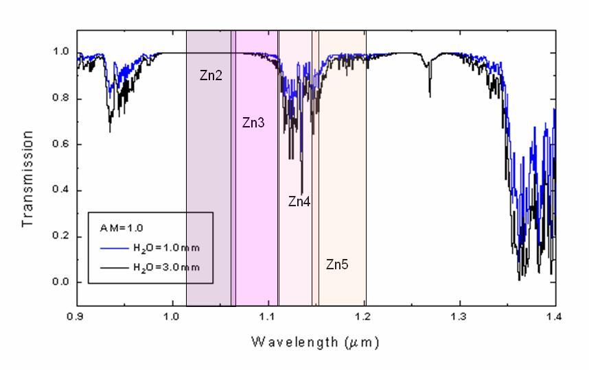
82 -82-

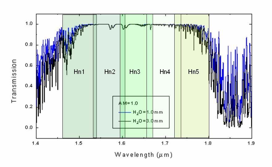
83 -83-

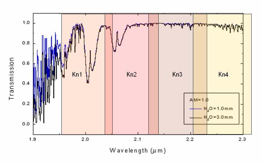
84 -84-