Ancient Admixture in Human History

Transcription

1 Genetics: Published Articles Ahead of Print, published on September 7, 2012 as /genetics Ancient Admixture in Human History Nick Patterson 1, Priya Moorjani 2, Yontao Luo 3, Swapan Mallick 2, Nadin Rohland 2, Yiping Zhan 3, Teri Genschoreck 3, Teresa Webster 3, and David Reich 1,2 1 Broad Institute of Harvard and MIT, Cambridge, MA Department of Genetics, Harvard Medical School, Boston, MA Affymetrix, Inc., 3420 Central Expressway, Santa Clara, CA ABSTRACT Population mixture is an important process in biology. We present a suite of methods for learning about population mixtures, implemented in a software package called AD- MIXTOOLS, that support formal tests for whether mixture occurred, and make it possible to infer proportions and dates of mixture. We also describe the development of a new single nucleotide polymorphism (SNP) array consisting of 629,433 sites with clearly documented ascertainment that was specifically designed for population genetic analyses, and that we genotyped in 934 individuals from 53 diverse populations. To illustrate the methods, we give a number of examples where they provide new insights about the history of human admixture. The most striking finding is a clear signal of admixture into northern Europe, with one ancestral population related to present day Basques and Sardinians, and the other related to present day populations of northeast Asia and the Americas. This likely reflects a history of admixture between Neolithic migrants and the indigenous Mesolithic population of Europe, consistent with recent analyses of ancient bones from Sweden and the sequencing of the genome of the Tyrolean Iceman. 1 Copyright 2012.

2 Running head: Ancient Admixture Keywords: Population genetics; Admixture; SNP array Corresponding Author: Dr. Nick J. Patterson Broad Institute 7 Cambridge Center Cambridge, MA Tel: (617) nickp@broadinstitute.org 2

3 INTRODUCTION Admixture between populations is a fundamental process that shapes genetic variation and disease risk. For example, African Americans and Latinos derive their genomes from mixtures of individuals who trace their ancestry to divergent populations. Study of the ancestral origin of the admixed individuals provides an opportunity to infer the history of the ancestral groups, some of whom may no longer be extant. The two main classes of methods in this field are local ancestry based methods and global ancestry based methods. Local ancestry based methods such LAMP (SANKARARAMAN et al. (2008)), HAPMIX (PRICE et al. (2009)) and PCADMIX (BRIS- BIN (2010)) deconvolve ancestry at each locus in the genome and provide individual-level information about ancestry. While these methods provide valuable insights into the recent history of populations, they have reduced power to detect older events. The most commonly used methods for studying global ancestry are Principal Component Analysis (PCA) (PATTERSON et al. (2006)) and model based clustering methods such as STRUCTURE (PRITCHARD et al. (2000)) and AD- MIXTURE (ALEXANDER et al. (2009)). While these are powerful tools for detecting population substructure, they do not provide any formal tests for admixture (the patterns in data detected using these methods can be generated by multiple population histories). For instance, NOVEMBRE et al. (2008) showed that Isolation-by-Distance can generate PCA gradients that are similar to those that arise from long-distance historical migrations, making PCA results difficult to interpret from a historical perspective. STRUCTURE/ADMIXTURE results are also difficult to interpret historically, because these methods work either without explicitly fitting a historical model, or by fitting a model that assumes that all the populations have radiated from a single ancestral group, which is 3

4 unrealistic. An alternative approach is to make explicit inferences about history by fitting phylogenetic treebased models to genetic data. A limitation of this approach, however, is that many of these methods do not allow for the possibility of migrations between groups, whereas most human populations derive ancestry from multiple ancestral groups. Indeed there are only a handful examples of human groups extant today, in which there is no evidence of genetic admixture. In this paper, we describe a suite of methods that formally test for a history of population mixture and allow researchers to build models of population relationships (including admixture) that fit genetic data. These methods are inspired by the ideas by CAVALLI-SFORZA and EDWARDS (1967) who fit phylogenetic trees of population relationships to the F st values measuring allele frequency differentiation between pairs of populations. Later studies by THOMPSON (1975); LATHROP (1982); WADDELL and PENNY (1996); BEERLI and FELSENSTEIN (2001) are more similar in spirit to our methods, in that they describe frameworks for fitting population mixture events (not just simple phylogenetic trees) to the allele frequencies observed in multiple populations, though the technical details are quite different from our work. In what follows we describe five methods: the 3-population test, D-statistics, F 4 ratio estimation, admixture graph fitting and rolloff. These have been introduced in some form in earlier papers (REICH et al., 2009; GREEN et al., 2010; DURAND et al., 2011; MOORJANI et al., 2011) but not coherently together, and with the key material placed in supplementary sections, making it difficult for readers to understand the methods and their scope. We also release a software package, ADMIXTOOLS, that implements these five methods for users interested in applying them to studies of population history. The first four techniques are based on studying patterns of allele frequency correlations across populations. The 3-population test is a formal test of admixture and can provide clear evidence of admixture, even if the gene flow events occurred hundreds of generations ago. The 4-population 4

5 test implemented here as D-statistics is also a formal test for admixture, which can not only provide evidence for admixture but also provide some information about the directionality of the gene flow. F 4 ratio estimation allows inference of the mixing proportions of an admixture event, even without access to accurate surrogates for the ancestral populations. However, this method demands more assumptions about the historical phylogeny. Admixture graph fitting allows one to build a model of population relationships for an arbitrarily large number of populations simultaneously, and to assess whether it fits the allele frequency correlation patterns among populations. Admixture graph fitting has some similarities to the TreeMix method of PICKRELL and PRITCHARD (2012) but differs in that TreeMix allows users to automatically explore the space of possible models and find the one that best fits the data (while our method does not), while our method provides a rigorous test for whether a proposed model fits the data (while TreeMix does not). It is important to point out that all four of the methods described in the previous paragraph measure allele frequency correlations among populations using the f -statistics and D -statistics that we define precisely in what follows. The expected values of these statistics are functions not just of the demographic history relating the populations, but also of the way that the analyzed polymorphisms were discovered (the so-called ascertainment process ). In principle, explicit inferences about the demographic history of populations can be made using the magnitudes of allele frequency correlation statistics, an idea that is exploited to great advantage by DURAND et al. (2011); however, for this approach to work, it is essential to analyze sites with rigorously documented ascertainment, as are available for example from whole genome sequencing data. Here our approach is fundamentally different in that we are focusing on tests for a history of admixture that assess whether particular statistics are consistent with 0. The expectation of zero in the absence of admixture is robust to all but the most extreme ascertainment processes, and thus these methods provide valid tests for admixture even using data from SNP arrays with complex ascertainment. We show this robustness both by simulation and with examples on real data, and also in some simple scenarios, 5

6 we demonstrate this theoretically.. Furthermore, we show that ratios of f-statistics can provide precise estimates of admixture proportions that are robust to both details of the ascertainment and to population size changes over the course of history, even if the f-statistics in the numerator and denominator themselves have magnitudes that are affected by ascertainment. The fifth method that we introduce in this study, rolloff, is an approach for estimating the date of admixture which models the decay of admixture linkage disequilibrium in the target population. Rolloff uses different statistics than those used by haplotype based methods such as STRUCTURE (PRITCHARD et al., 2000) and HAPMIX (PRICE et al., 2009). The most relevant comparison is to the method of POOL and NIELSEN (2009), who like us are specifically interested in learning about history, and who estimate population mixture dates by studying the distribution of ancestry tracts inherited from the two ancestral populations. A limitation of the POOL and NIELSEN (2009) approach, however, is that it assumes that local ancestry inference is perfect, whereas in fact most local ancestry methods are unable to accurately infer the short ancestry tracts that are typical for older dates of mixture. Precisely for these reasons, the HAPMIX paper cautions against using HAPMIX for date estimation (PRICE et al., 2009). In contrast, rolloff does not require accurate reconstruction of the breakpoints across the chromosomes or data from good surrogates for the ancestors, making it possible to interrogate older dates. Simulations that we report in what follows show that rolloff can produce unbiased and quite accurate estimates for dates up to 500 generations in the past. 6

7 METHODS AND MATERIALS Throughout this paper, unless otherwise stated, we consider biallelic markers only, and we ignore the possibility of recurrent or back mutations. Our notation in this paper is that we write f 2 (and later f 3, f 4 ) for statistics: empirical quantities that we can compute from data, and F 2 (and later F 3, F 4 ) for corresponding theoretical quantities that depend on an assumed phylogeny (and the ascertainment). We define drift as the frequency change of an allele along a graph edge (hence drift between 2 populations A and B is a function of the difference in the allele frequency of polymorphisms in A and B). The 3-population test and introduction of f-statistics We begin with a description of the 3-population test. First some theory. Consider the tree of Figure 1a. We see that the path from C to A and the path from C to B just share the edge from C to X. Let a, b, c be expected allele frequencies in the populations A, B, C respectively, at a single polymorphism. Define F 3 (C; A, B) = E[(c a )(c b )] 7

8 We similarly, in an obvious notation define F 2 (A, B) = E[(a b ) 2 ] F 4 (A, B; C, D) = E[(a b )(c d )] Choice of the allele does not affect any of F 2, F 3, F 4 as choosing the alternate allele simply flips the sign of both terms in the product. We refer to F 2 (A, B) as the branch length between populations A and B. We use these branch lengths in admixture graph fitting for graph edges. Our F values should be viewed as population parameters, but we note that they depend both on the demography and choice of SNPs. In Box 1 we give formulae that use sample frequencies and that yield unbiased estimates of the corresponding F parameters. The unbiased estimates of F computed using these formulae at each marker are then averaged over many markers to form our f-statistics. The results that follow hold rigorously if we identify the polymorphisms we are studying in an outgroup (that is, we select SNPs based on patterns of genetic variation in populations that all have the same genetic relationship to populations A, B, C). Since only markers with variation in A, B, C are relevant to the analysis, then by ascertaining in an outgroup we ensure that our markers are polymorphic in the root population of A, B, C. Later on, we discuss how other strategies for ascertaining polymorphisms would be expected to affect our results. In general, our tests for admixture and estimates of admixture proportion are strikingly robust to the ascertainment processes that are typical for human SNP array data, as we verify both by simulations and by empirical analysis. Suppose the allele frequency of a SNP is r at the root. In the tree of Figure 1a, let a, b, c, x, r be 8

9 allele frequencies in A, B, C, X, R. Condition on r. Then E[(c a )(c b )] = E[(c x + x a )(c x + x b )] = E[(c x ) 2 ] 0 since E[a x ] = x, and E[x b ] = E[r b (r x )] = 0. If the phylogeny has C as an outgroup (switching B, C in Figure 1a), then a similar argument shows that E[(c a )(c b )] = E[(r c ) 2 ] + E[(r x ) 2 ] 0 There is an intuitive way to think about the expected values of f-statistics, which relies on tracing the overlap of genetic drift paths between the first and second terms in the quadratic expression, as illustrated in Box 2. For example, E[(c a )(c b )] can only be negative if population C has ancestry from populations related to both A and B. Only in this case are there paths between C and A and C and B that also take opposite drift directions through the tree (Figure 1c and Figure2), which contributes to a negative expectation for the statistics. The observation of a significantly negative value of f 3 (C; A, B) is thus evidence of complex phylogeny in C. We prove this formally in the Appendix (Theorem 1). In the Appendix, we also relax our assumptions about the ascertainment process, showing that F 3 is guaranteed to be positive if C is unadmixed under quite general conditions; for example, polymorphic in the root R and in addition ascertained as polymorphic in any of A, B, C. It is important to recognize, however, that a history of admixture does not always result in a negative f 3 (C; A, B)-statistic. If population C has experienced a high degree of population-specific drift (perhaps due to founder events after admixture), it can mask the signal so that f 3 (C; A, B) might not be negative. An important feature of this test is that it definitively shows that the history of mixture occurred in population C; a complex history for A or B cannot produce negative F 3 (C; A, B). To explain 9

10 why this is so, we recapitulate material from REICH et al. (2009, Supplementary Material). If population A is admixed then if we pick an allele of A, it must have originated in one of the admixing populations. Pick alleles α, β from populations A and B and γ 1, γ 2 independently from C, coding 1 for a reference allele, 0 for a variant, etc. Thus, F 3 (C; A, B) = E[(γ 1 α)(γ 2 β)]. Suppose population A is admixed, B and C are not admixed. The allele α sampled from population A can take more than one path through the ancestral populations. F 3 (C; A, B) can then be computed as a weighted average over the possible phylogenies, in all of which the quantity has a positive expectation because A and B are now unadmixed (Box 2 and Figure 2). In conclusion, the diagram makes it visually evident that if F 3 (C; A, B) < 0 then population C itself must have a complex history. Additivity of F 2 along a tree branch In this paper we are considering generalizations of phylogenetic trees and graph edges indicate that one population is a descendant of another. Consider the phylogenetic tree in Figure 1b, and a marker polymorphic at the root. Drift on a given edge is a random variable with mean 0. For if A B is a graph edge, with corresponding allele frequencies a, b E[b a ] = a This is the martingale property of allele frequency diffusion. Drifts on 2 distinct edges of a tree are orthogonal, where orthogonality of random variables X, Y simply means that E[XY ] = 0. In our context this means that the drifts on distinct edges have mean 0 and are uncorrelated. A valuable feature of our F -statistics definition is that branch lengths on the tree (as defined by F 2 ) are additive. 10

11 We illustrate this with an example from human history (Figure 1b). (We note that all examples in this paper refer to human history, although the methods should apply equally well to other species.) In this example, A, and C are present-day populations that split from an ancestral population X. B is an ancestral population to C. For instance, A might be modern Yoruba, C a European population, and B an ancient population, perhaps a sample from archaeological material of a population that existed thousands of years ago. We assume here that we ascertain in an outgroup (implying polymorphism at the root), and again assume neutrality and that we can ignore recurrent or back mutations. Then we mean by additivity that F 2 (A, C) = F 2 (A, B) + F 2 (B, C) For E[(a c ) 2 ] = E[(a b + b c ) 2 ] = E[(a b ) 2 ] + E[(b c ) 2 ] + 2E[(a b )(b c )] but the last term is 0 since the change in allele frequencies ( drifts ) X A, X B, B C are all uncorrelated. We remark that our F 2 -distance resembles the familiar F st, but is not the same. In particular parts of a graph that are far from the root (in genetic drift distance) have F 2 reduced. Some insight into this effect is given by considering the simple graph: R τ 1 A τ 2 B where τ 1, τ 2 are drift times on the standard diffusion timescale (2 random alleles of B have proba- 11

12 bility e τ 2 that they have not coalesced in the ancestral population A). If r, a, b are allele frequencies in R, A, B respectively then F 2 (A, B) = E[(a b ) 2 ]. Write E r, E a for expectations conditional on population allele frequencies r, a. Then E a [(a b ) 2 ] = a (1 a )(1 e τ 2 ) (NEI, 1987, Chapter 13). Moreover E r [a (1 a )] = r (1 r )e τ 1. Hence F 2 (A, B) = E[r (1 r )e τ 1 (1 e τ 2 )] Informally the drift from R A shrinks F 2 (A, B) by a factor e τ 1. Thus expected drift is additive: F 2 (R, B) = F 2 (R, A) + F 2 (A, B) but the drift does depend on ascertainment. For a given edge, the more distant the root, the smaller the drift. A loose analogy is projecting a curved surface, such as part of the globe, into a plane. Locally all is well, but any projection will cause distortion in the large. Additivity in f 2 distances is all we require in what follows. We note that there is no assumption here that population sizes are constant along a branch edge, and so we are not assuming linearity of branch lengths in time. Expected values of our f-statistics We can calculate expected values for our f-statistics, at least for simple demographic histories that involve population splits and admixture events. We will assume that genetic drift events on distinct edges are uncorrelated, which as mentioned before will be true if we ascertain in an outgroup, and our alleles are neutral. 12

13 We give an illustration for f 3 -statistics. Consider the demography shown in Figure 1c. Populations E, F split from a root population R. G then was formed by admixture in proportions α : β (β = 1 α). Modern populations A, B, C are then formed by drift from E, F, G. We want to calculate the expected value of f 3 (C; A, B). Assume that our ascertainment is such that drifts on distinct edges are orthogonal, which will hold true if we ascertained the markers in an outgroup. We recapitulate some material from (REICH et al., 2009, Supplementary S2, section 2.2). As before let a, b, c be population allele frequencies in A, B, C, and let g be the allele frequency in G and so on. F 3 (C; A, B) = E[(c a )(c b )] We see by orthogonality of drifts that F 3 (C; A, B) = E[(g a )(g b )] + E[(g c ) 2 ] which we will write as F 3 (C; A, B) = F 3 (G; A, B) + F 2 (C, G) (1) Now, label alleles at a marker 0, 1. Then picking chromosomes from our populations independently we can write F 3 (G; A, B) = E[(g 1 a 1 )(g 2 b 1 )] where a 1, b 1 are alleles chosen randomly in populations A, B and g 1, g 2 are alleles chosen randomly and independently in population G. Similarly, we define e 1, e 2, f 1 and f 2. However g 1 originated 13

14 from E with probability α and so on. Thus: F 3 (G; A, B) = E[(g 1 a 1 )(g 2 b 1 )] = α 2 E[(e 1 a 1 )(e 2 b 1 )] + + β 2 E[(f 1 a 1 )(f 2 b 1 )] + + αβe[(e 1 a 1 )(f 1 b 1 )] + + αβe[(f 1 a 1 )(e 1 b 1 )] where a 1, a 2 are independently picked from E and b 1, b 2 from F. The first 3 terms vanish. Further E[(f 1 a 1 )(e 1 b 1 )] = E[(e 1 f 1 ) 2 ] This shows that under our assumptions of orthogonal drift on distinct edges, that F 3 (C; A, B) = F 2 (C, G) αβf 2 (E, F ) (2) It might appear that Figure 1c is too restricted, as it assumes that the admixing populations E, F are ancestral to A, B and that we should consider the more general graph shown in Figure 1d. But it turns out that using our f-statistics alone (and not the more general allelic spectrum) that even if α, β are known, we can only obtain information about α 2 u + β 2 v + w Thus in fitting Admixture Graphs to f-statistics, we can, without loss of generality, fit all the genetic drift specific to the admixed population on the lineage directly ancestral to the admixed 14

15 population (the lineage leading from C to G in Figure 1c). The outgroup case Care though is needed in interpretation. Consider Figure 1e. Here a similar calculation to the one just given shows (again assuming orthogonality of drift on each edge) that F 3 (C; A, Y ) = F 2 (C, G) + β 2 F 2 (F, X) αβf 2 (E, X) (3) Note that Y has little to do with the admixture into C and we will obtain the same F 3 value for any population Y that splits off from A more anciently than X. We call this case, where we have apparent admixture between A and Y, the outgroup case, and it needs to be carefully considered when recovering population relationships. Estimates of mixing proportions We would like to estimate, or at least bound, the mixing proportions that have resulted in the ancestral population of C. With further strong assumptions on the phylogeny we can get quite precise estimates even without accurate surrogates for the ancestral populations (see REICH et al. (2009) and the F 4 ratio estimation that we describe below, for examples). Also if we have data from populations that are accurate surrogates For the ancestral admixing population (and we can ignore the drift post admixture), the problem is much easier. For instance in PATTERSON et al. (2010) we give an estimator that works well even when the sample sizes of the relevant populations are small, 15

16 and we have multiple admixing populations whose deep phylogenetic relationships we may not understand. Here we show a method that obtains useful bounds, without requiring full knowledge of the phylogeny, though the bounds are not very precise. Note that although our 3-population test remains valid even if the populations A, B are admixed, the mixing proportions we are calculating are not meaningful unless the assumed phylogeny is at least roughly correct. Indeed even discussing mixing from an ancestral population of A hardly makes sense if A is admixed itself subsequent to the admixing event in C. This is discussed further when we present data from Human Genome Diversity Panel (HGDP) populations. In much of the work in this paper, we are analyzing some populations A, B, C and need an outgroup which split off from the ancestral population of A, B, C before the population split of A, B. For example in Figure 1e, Y is such an outgroup. Usually, when studying a group of populations within a species, a plausible outgroup can be proposed. The outgroup assumption can then be checked using the methods of this paper, by adding an individual from a more distantly related population, which can be treated as a second outgroup. For instance with human populations from Eurasia, Yoruba or San Bushmen from sub-saharan Africa 1 will often be plausible outgroups. Our second outgroup here is simply being used to check a phylogenetic assumption in our primary analysis, and we do not require polymorphism at the root for this narrow purpose. Chimpanzee is always a good second outgroup for studies of humans. Consider the phylogeny of Figure 1f. Here α, β are mixing parameters (α + β = 1) and we show drift distances along the graph edges. Note that here we use a, b,... as branch lengths (F 2 distances), not sample or population allele frequencies as we do elsewhere in this paper. Thus for 1 There is no completely satisfactory term for the Khoisan peoples of southern Africa; see BARNARD (1992, introduction) for a sensitive discussion. We prefer Bushmen following Barnard. However, the standard name for the HGDP Bushmen sample is San in the genetic literature (for example CANN et al. (2002)) and we use this specifically to refer to these samples. 16

17 example F 2 (O, X) = u. Now we can obtain estimates of: Z 0 = u = F 3 (O; A, B) Z 1 = u + αa = F 3 (O; A, C) Z 2 = u + βb = F 3 (O; B, C) Z 3 = u + a + f = F 2 (O; A) Z 4 = u + b + g = F 2 (O; B) Z 5 = u + h + α 2 (a + d) + β 2 (b + e) = F 2 (O; C) We also have estimates of F = h αβ(a + b) = F 3 (C; A, B) Set Y i = Z i Z 0, i = which eliminates u. This shows that any population O which is a true outgroup should (up to statistical noise) give similar estimates for Y i (Figure 1f). We have 3 inequalities: α Y 1 /Y 3 β Y 2 /Y 4 αβ(a + b) F Using αa = Y 1, βb = Y 2 we can rewrite these as: Y 1 /Y 3 α 1 Y 2 /Y 4 α(y 2 Y 1 ) F Y 1 giving lower and upper bounds on α, which we write as α L, α U in the tables of results that follow. 17

18 These bounds can be computed by a program qpbound in the ADMIXTOOLS software package that we make available with this paper. Although these bounds will be nearly invariant to choices of the outgroup O, choices for the source populations A, B may make a substantial difference. We give an example in a discussion of the relationship of Siberian populations to Europeans. In principle we can give standard errors for the bounds, but these are not easily interpretable, and we think that in most cases systematic errors (for instance that our phylogeny is not exactly correct) are likely to dominate. We observe that in some cases the lower bound exceeds the upper, even when the Z-score for admixture of population C is highly significant. We interpret this as suggesting that our simple model for the relationships of the three populations is wrong. A negative Z-score indeed implies that C has a complex history, but if A or B also have complex histories, then a recovered mixing coefficient α has no real meaning. Estimation and normalization With all our f-statistics it is critical that we can compute unbiased estimates of the population F -parameter for a single SNP, with finite sample sizes. Without that, our estimates will be biased, even if we average over many unlinked SNPs. The explicit formulae for f 2, f 3, f 4 we present in Box 1 (previously given in REICH et al. (2009, Supplementary Material)) are in fact minimum variance unbiased estimates of the corresponding F -parameters, at least for a single marker. The expected (absolute) values of an f-statistic such as f 3 strongly depends on the distribution of the derived allele frequencies of the SNPs examined; for example, if many SNPs are present that have a low average allele frequency across the populations being examined, then the magnitude 18

19 of f 3 will be reduced. To see this, suppose that we are computing f 3 (C; A, B), and as before a, b, c are population frequencies of an allele in A, B, C. If the allele frequencies are small, then it is obvious that the expected value of f 3 (C; A, B) will be small in absolute magnitude as well. Importantly, however, the sign of an f-statistic is not dependent on the absolute magnitudes of the allele frequencies (all that it depends on is the relative magnitudes across the populations being compared). Thus, a significant deviation of an f-statistic from 0 can serve as a statistically valid test for admixture, regardless of the ascertainment of the SNPs that are analyzed. However, to reduce the dependence of the value of the f 3 statistic on allele frequencies for some of our practical computations, in all of the empirical analyses we report below, we normalize using an estimate for each SNP of the heterozygosity of the target population C. Specifically, for each SNP i, we compute unbiased estimates ˆT i, ˆB i of both T i = (c a )(c b ) B i = 2c (1 c ) Now we normalize our f 3 -statistic computing f 3 = i ˆT i i ˆB i This greatly reduces the numerical dependence of f 3 on the allelic spectrum of the SNPs examined, without making much difference to statistical significance measures such as a Z-score. We note that we use f 3 and f 3 interchangeably in many places in this paper. Both of these statistics give qualitatively similar results and thus if the goal is only to test if f 3 has negative expected value then the inference should be unaffected. D-statistics 19

20 The D-statistic test was first introduced in (GREEN et al., 2010) where it was used to formally evaluate whether modern humans have some Neandertal ancestry. Further theory and applications of D-statistics can be found in REICH et al. (2010) and DURAND et al. (2011). A very similar statistic f 4 was used to provide evidence of admixture in India (REICH et al., 2009), where we called it a 4-population test. The D-statistic was also recently used as a convenient statistic for studying locus-specific introgression of genetic material controlling coloration in Heliconius butterflies (DASMAHAPATRA et al., 2012). Let W, X, Y, Z be 4 populations, with a phylogeny that corresponds to the unrooted tree of Figure 3a. For SNP i suppose variant population allele frequencies are w, x, y, z respectively. Choose an allele at random from each of the 4 populations. Then we define a BABA event to mean that the W and Y alleles agree, and the X and Z alleles agree, while the W and X alleles are distinct. We define an ABBA event similarly, now with the W and Z alleles in agreement. Let Num i and Den i be the numerator and denominator of the statistic: Num i = P (BABA) P (ABBA) = (w x )(y z ) Den i = P (BABA) + P (ABBA) = (w + x 2w x )(y + z 2y z ) For SNP data these values can be computed using either population or sample allele frequencies. DURAND et al. (2011) showed that replacing population allele frequencies (w, y etc) by the sample allele frequencies yields unbiased estimates of Num i, Den i. Thus if w, x, y, z are sample allele frequencies we define: ˆNum i = (w x)(y z) ˆDen i = (w + x 2wx)(y + z 2yz) 20

21 and, in a similar spirit to our normalized f 3 -statistic f 3 we define the D-statistic D(W, X; Y, Z) as D = i ˆNum i ˆDen i i summing both the numerator and denominator over many SNPs and only then taking the ratio. If we ascertain in an outgroup, then if (W, X) and (Y, Z) are clades in the population tree, it is easy to see that E[Num i ] = 0. We can compute a standard error for D using the weighted block jackknife (BUSING et al., 1999). The number of standard errors that this quantity is from zero forms a Z-score, which is approximately normally distributed and thus yields a formal test for whether (W, X) indeed forms a clade. More generally, if the relationship of the analyzed populations is as shown in Figure 3c or Figure 3d and we ascertain in an outgroup or in {W, X} then D should be zero up to statistical noise. The reason is that if U is the ancestral population to Y, Z and u, y, z are population allele frequencies in U, Y, Z, then E[y z u ] = E[y u ] E[z u ] = 0. Here there is no need to assume polymorphism at the root of the tree, as for a SNP to make a non-zero contribution to D we must have polymorphism at both {Y, Z} and {W, X}. If the tree assumption is correct, drift between Y, Z and between W, X are independent so that E[Num i ] = 0. Thus testing whether D is consistent with zero constitutes a test for whether (W, X) and (Y, Z) are clades in the population tree. As mentioned earlier, D-statistics are very similar to the 4-population test statistics introduced in REICH et al. (2009). The primary difference is in the computation of the denominator of D. For statistical estimation, and testing for treeness, the D-statistics are preferable, as the denominator of D, the total number of ABBA and BABA events, is uninformative for whether a tree phylogeny is supported by the data, while D has a natural interpretation: the extent of the deviation on 21

22 a normalized scale from -1 to 1. As an example, let us assume that two human Eurasian populations A, B are a clade with respect to West Africans (Yoruba). Assume the phylogeny shown in Figure 3b, and that we ascertain in an outgroup to A, B. Then E[D(Chimp, Y oruba; A, B)] = 0 F 4 Ratio Estimation F 4 ratio estimation, previously referred to as f 4 ancestry estimation in REICH et al. (2009), is a method for estimating ancestry proportions in an admixed population, under the assumption that we have a correct historical model. Consider the phylogeny of Figure 4. The population X is an admixture of populations B and C (possibly with subsequent drift). We have genetic data from populations A, B, X, C, O. Since F 4 (A, O; C, C) = 0 it follows that F 4 (A, O; X, C) = αf 4 (A, O; B, C) = αf 4 (A, O; B, C) (4) Thus an estimate of α is obtained as: ˆα = f 4(A, O; X, C) f 4 (A, O; B, C) (5) where the estimates in both numerator and denominator are obtained by summing over many SNPs. 22

23 As we can obtain unbiased f 4 -statistics by sampling a single allele from each population, we can apply this test to sequence data, where we pick a single allele, from a high quality read, for all relevant populations at each polymorphic site. In practice this must be done with care as both sequencing error that is correlated between samples, and systematic misalignment of reads to a reference sequence, can distort the statistics. Examples of F 4 Ratio Estimation REICH et al. (2009) provide evidence that most human South Asian populations can be modeled as a mixture of Ancestral North Indians (ANI) and Ancestral South Indians (ASI) and that if we set, using the labeling above: Label A B X C O Population Adygei CEU (HapMap European Americans) Indian (Many populations) Onge (Indigenous Andamanese) Papuan (Dai and HapMap Yoruba West Africans also work) we get estimates of the mixing coefficients that are robust, have quite small standard errors and are in conformity with other estimation methods. See (REICH et al., 2009, Supplementary S5) for further details. As another example, in REICH et al. (2010) and GREEN et al. (2010) evidence was given that there was gene flow (introgression) from Neandertals into non-africans. Further, a sister group to Neandertals, Denisovans represented by a fossil from Denisova cave, Siberia, shows no evidence of having contributed genes to present-day humans in mainland Eurasia (REICH et al., 2010, 2011). 23

24 The phylogeny is that of Figure 4 if we set: Label A B X C O Population Denisova Neandertal French (or almost any population from the Eurasian mainland) Yoruba Chimpanzee Here B are the population of Neandertals that admixed, which form a clade with the Neandertals from Vindija that were sequenced GREEN et al. (2010). So for this example, we obtain an estimate of α, the proportion of Neandertal gene flow into French as.022 ±.007 (see REICH et al. (2010, SI8) for more detail). Simulations to test the accuracy of f- and D-statistic based historical inferences We carried out coalescent simulations of 5 populations related according to Figure 4, using ms (HUDSON (2002)). Detailed information about the simulations is given in Appendix 1. Table 2 shows that using 3-population test, D-statistics, and F 4 ratio estimation, we reliably detect mixture events and obtain accurate estimates of mixture proportions, even for widely varied demographic histories and strategies for discovering polymorphisms. The simulations also document important features of our methods. As mentioned earlier, the only case where the f 3 -statistic for a population that is truly admixed fails to be negative is when the population has experienced a high degree of population-specific genetic drift after the admixture occurred. Further, the D-statistics only show a substantial deviation from 0 when an admixture 24

25 event occurred in the history of the 4 populations contributing to the statistic. Finally, the estimates of admixture proportions using F 4 ratio estimation are accurate for all ascertainment strategies and demographies. Effect of ascertainment process on f- and D-statistics So far, we have assumed that we have sequence data from all populations and ascertainment is not an issue. However, the ascertainment of polymorphisms (for example, enriching the set of analyzed SNPs for Ancestry Informative Markers) can modulate the magnitudes of F 3, F 4 and D. Empirically, we observe that in commercial SNP arrays developed for genome-wide association studies (like Affymetrix 6.0 and Illumina 610-Quad), ascertainment does indeed affect the observed magnitudes of these statistics, but importantly, does not cause them to be biased aware from zero if this is their expected value in the absence of complex ascertainment (e.g. for complete genome sequencing data). This is key to the robustness of our tests for admixture: since our tests are largely based on evaluating whether particular f- or D-statistics are consistent with zero, and SNP ascertainment almost never causes a deviation from zero, the ascertainment process does not appear to be contributing to spuriously significant signals of admixture. We have verified this through two lines of analysis. First, we carried out simulations showing that tests of admixture (as well as F 4 ratio estimation) perfomed using these methods are robust to very different SNP ascertainment strategies (Table 2). Second, we report analyses of data from a new SNP array with known ascertainment that we designed specifically for studies of population history. Even when we use radically different ascertainment schemes, and even when we use widely-used commercial SNP arrays, inferences about history are indistinguishable (Table 8). Admixture graph fitting 25

26 We next describe qpgraph, our tool for building a model of population relationships from f- statistics. We first remark that given n populations P 1, P 2,..., P n then 1. The f-statistics (f 2, f 3 and f 4 ) span a linear space V F of dimension ( n 2). 2. All f-statistics can be found as linear sums of statistics f 2 (P i ; P j ) 1 i < j. 3. Fix a population (say P 1 ). Then all f-statistics can be found as linear sums of statistics f 3 (P 1 ; P i, P j ), f 2 (P 1, P i ) 1 < i < j. These statements are true, both for the theoretical F -values, and for our f-statistics, at least when we have no missing data, so that for all populations our f-statistics are computed on the same set of markers. Requirements (2) and (3) describe bases for the vector space V F. We usually find the basis of (3) to be the most convenient computationally. More detail can be found in (REICH et al., 2009, Supplement paragraph 2.3). Thus choose a basis. From genotype data we can calculate 1. f-statistics on the basis. Call the resulting ( n 2) long vector f. 2. An estimated error covariance Q of f using the weighted block jackknife (BUSING et al., 1999). Now, given a graph topology, as well as graph parameters (edge values and admixture weights) we can calculate g, the expected value of f. A natural score function is S 1 (g) = 1 2 (g f) Q 1 (g f) (6) 26

27 an approximate log-likelihood. Note that non-independence of the SNPs is taken into account by the jackknife. A technical problem is that for n large our estimate Q of the error covariance is not stable. In particular, the smallest eigenvalue of Q may be unreasonably small. This is a common issue in multivariate statistics. Our program qpgraph allows a least squares option with a score function S 2 (g) = 1 2 i (g i f i ) 2 (Q ii + λ) where λ is a small constant introduced to avoid numerical problems. The score S 2 is not basis independent, but in practice seems robust. (7) Maximizing S 1 or S 2 is straightforward, at least if n is moderate, which is the only case in which we recommend using qpgraph. We note that given the admixture weights, both score functions S 1, S 2 are quadratic in the edge lengths, and thus can be maximized using linear algebra. This reduces the maximization to the choice of admixture weights. We use the commercial routine nag opt simplex from the Numerical Algorithms Group ( pdf/e04/e04ccc.pdf), which has an efficient implementation of least squares. Users of qp- Graph will need to have access to nag, or substitute an equivalent subroutine. Interpretation and limitations of qpgraph 1. A major use of qpgraph is to show that a hypothesized phylogeny must be incorrect. This generalizes our D-statistic test, which is testing a simple tree on 4 populations. 2. After fitting parameters, study of which f-statistics fit poorly can lead to insights as to how the model must be wrong. 3. Overfitting can be a problem, especially if we hypothesize many admixing events, but only have data for a few populations. 27

28 Simulations validate the performance of qpgraph We show in Figure 5 an example where we simulated a demography with 5 observed populations Out, A, B, C, X and one admixture event. We simulated 50, 000 unlinked SNPs, ascertained as heterozygous in a single diploid individual from the outgroup Out. Sample sizes were 50 in all populations and the historical population sizes were all taken to be 10, 000. We show that we can accurately recover the drift lengths and admixture proportions using qpgraph. rolloff Our fifth technique rolloff, studies the decay of admixture linkage disequilibrium with distance to infer the date of admixture. Importantly, we do not consider multi-marker haplotypes, but instead study the joint allelic distribution at pairs of markers, where the markers are stratified into bins by genetic distance. This method was first introduced in MOORJANI et al. (2011) where it was used to infer the date of sub-saharan African gene flow into southern Europeans, Levantines and Jews. Suppose we have an admixed population and for simplicity assume that the population is homogeneous (which usually implies that the admixture is not very recent). Let us also assume that admixture occurred over a very short time span (pulse admixture model), and since then our admixed (target) population has not experienced further large scale immigration from the source populations. Call the two admixing (ancestral) populations A, B. Consider two alleles on a chromosome in an admixed individual at loci that are a distance d Morgans apart. Then 28

29 n generations after admixture, with probability e nd the two alleles belonged, at the admixing time, to a single chromosome. Suppose we have a weight function w at each SNP that is positive when the variant allele has a higher frequency in population A than in B and negative in the reverse situation. For each SNP s, let w(s) be the weight for SNP s. For every pair of SNPs s 1, s 2, we compute an LD-based score z(s 1, s 2 ) which is positive if the two variant alleles are in linkage disequilibrium; that is, they appear on the same chromosome more often than would be expected assuming independence. For diploid unphased data, which is what we have here, we simply let v 1, v 2 be the vectors of genotype counts of the variant allele, dropping any samples with missing data. Let m be the number of samples in which neither s 1 or s 2 has missing data. Let ρ be the Pearson correlation between v 1, v 2. We apply a small refinement, insisting that m 4 and clipping ρ to the interval [ 0.9, 0.9]. Then we use Fisher s z-transformation: z = m 3 log 2 ( ) 1 + ρ 1 ρ which is known to improve the tail behavior of z. In practice this refinement makes little difference to our results. Now we form a correlation between our z-scores and the weight function. Explicitly, for a binwidth x, define the bin S(d), d = x, 2x, 3x,... by the set of SNP pairs (s 1, s 2 ), where: S(d) = {(s 1, s 2 ) d x < u 2 u 1 d} where u i is the genetic position of SNP s i. 29

30 Then we define A(d) to be the correlation coefficient A(d) = s 1,s 2 S(d) w(s 1)w(s 2 )z(s 1, s 2 ) [ s1,s2 S(d) (w(s 1)w(s 2 )) 2 s1,s2 S(d) (z(s 1, s 2 )) 2] 1/2 (8) Here in both numerator and denominator we sum over pairs of SNPs approximately d Morgans apart (counting SNP pairs into discrete bins). In this study, we set a bin-size of 0.1 centimorgans (cm) in all our examples. In practice, different choices of bin-sizes only qualitatively affect the results (MOORJANI et al. (2011)). Having computed A(d) over a suitable distance range, we fit A(d) A 0 e nd (9) by least squares and interpret n as an admixture date in generations. Equation 9 follows because a recombination event on a chromosome since admixture decorrelates the alleles at the two SNPs being considered, and e nd is the probability that no such event occurred. (Implicitly, we are assuming here that the number of recombinations over a genetic interval of d Morgans in n generations is Poisson distributed with mean nd. Because of crossover interference, this is not exact, but it is an excellent approximation for the d and n relevant here.) By fitting a single exponential distribution to the output, we have assumed a single pulse model of admixture. However, in the case of continuous migration we can expect the recovered date to lie within the time period spanned by the start and end of the admixture events. We further discuss rolloff date estimates in the context of continuous migration in applications to real data (below). We estimate standard errors using a weighted block jackknife (BUSING et al., 1999) where we 30

31 drop one chromosome in each run. Choice of weight function In many applications, we have access to two modern populations A, B which we can regard as surrogates for the true admixing populations, and in this context we can simply use the difference of empirical frequencies of the variant allele as our weight. For example, to study the admixture in African Americans, very good surrogates for the ancestral populations are Yoruba and North Europeans. However, a strength of rolloff is that it provides unbiased dates even without access to accurate surrogates for the ancestral populations. That is, rolloff is robust to use of highly divergent populations as surrogates. In cases when the ancestrals are no longer extant or data from the ancestrals are not available, but we have access to multiple admixed populations with differing admixture proportions (as for instance happens in India (REICH et al., 2009)), we can use the SNP loadings generated from principal component analysis (PCA) as appropriate weights. This also gives unbiased dates for the admixture events. Simulations to test rolloff We ran three sets of simulations. The goals of these simulations were: (1) To access the accuracy of the estimated dates, in cases for which data from accurate ancestral populations are not available. (2) To investigate the bias seen in MOORJANI et al. (2011). (3) To test the effect of genetic drift that occurred after admixture. We describe the results of each of these investigations in turn. 1. First, we report simulation results that test the robustness of inferences of dates of admixture 31

32 when data from accurate ancestral populations are not available. We simulated data for 20 individuals using phased data from HapMap European Americans (CEU) and HapMap West Africans (YRI), where the mixture date was set to 100 generations before present and the proportion of European ancestry was 20%. We ran rolloff using pairs of reference populations that were increasingly divergent from the true ancestral populations used in the simulation. The results are shown in Table 3 and are better than those of the rather similar simulations in MOORJANI et al. (2011). Here we use more SNPs (378K instead of 83K) and 20 admixed individuals rather than 10. The improved results likely reflect the fact that we are analyzing larger numbers of admixed individuals and SNPs in these simulations, which improves the accuracy of rolloff inferences by reducing sampling noise in the calculation of the Z-score. In analyzing real data, we have found that the accuracy of rolloff results improves rapidly with sample size; this feature of rolloff contrasts markedly with allele frequency correlation statistics like f-statistics where the accuracy of estimation increases only marginally as sample sizes increase above 5 individuals per population. 2. Second, we report simulation results investigating the bias seen in MOORJANI et al. (2011). MOORJANI et al. (2011) showed that low sample size and admixture proportion can cause a bias in the estimated dates. In our new simulations, we generated haplotypes for 100 individuals using phased data from HapMap European Americans (CEU) and HapMap West Africans (YRI), where the mixture date was between 50 and 800 generations ago (Figure 6) and the proportion of European ancestry was 20%. We ran rolloff with two sets of reference populations: (1) the true ancestral populations (CEU and YRI) and (2) the divergent populations Gujarati (F st (CEU, Gujarati) = 0.03 and Maasai (F st (YRI, Maasai) = 0.03). We show the results for one run and the mean date from each group of 10 runs in Figures 6a and 6b. These results show no important bias, and the date estimates, even in the more difficult case where we used Gujarati and Maasai as assumed ancestrals, are tightly clustered near the truth up to 500 generations (around 15,000 years). This shows that the bias is removed 32

33 with larger sample sizes. 3. The simulations reported above sample haplotypes without replacement, effectively removing the impact of genetic drift after admixture. To study the effect of drift post-dating admixture, we performed simulations using the MaCS coalescent simulator (CHEN et al. (2009)). We simulated data for one chromosome (100 Mb) for three populations (say, A, B and C). We set the effective population size (N e ) for all populations to 12,500, the mutation rate to per base pair per generation, and the recombination rate to per base pair per generation. Consider the phylogeny in Figure 1c. G is an admixed population that has 80%/20% ancestry from E and F, with an admixture time (t) set to be either 30, 100 or 200 generations before the present. Populations A, B, C are formed by drift from E, F, G respectively. F st (A, B) = 0.16 (similar to that of F st (Y RI, CEU)). We performed rolloff analysis with C as the target (n = 30) and A and B as the reference populations. We estimated the standard error using a weighted block jackknife where the block size was set to 10cM. The estimated dates of admixture were 28 ± 4, 97 ± 10 and 212 ± 19 corresponding the true admixture dates of 30, 100 and 200 generations respectively. This shows that the estimated dates are not measurably affected by genetic drift post-dating the admixture event. A SNP array designed for population genetics We conclude our presentation of our methods by describing a new experimental resource and publicly available dataset that we have generated for facilitating studies of human population history, and that we use in many of the applications that follow. For studies that aim to fit models of human history to genetic data, it is highly desirable to have an exact record of how polymorphisms were chosen. Unfortunately, conventional SNP arrays 33

34 developed for medical genetics have a complex ascertainment process that is nearly impossible to reconstruct and model (but see WOLLSTEIN et al. (2010)). While the methods reported in our study are robust in theory and also in to simulation to a range of strategies for how polymorphisms were ascertained (Table 2), we nevertheless wished to empirically validate our findings on a dataset without such uncertainties. Here, we report on a novel SNP array that we developed that is now released as the Affymetrix Human Origins array. This includes 13 panels of SNPs each ascertained in a rigorously documented way that is described in the Supplementary Note, allowing users to choose the one most useful for a particular analysis. The first 12 are based on a strategy used in KEINAN et al. (2007), discovering SNPs as heterozygotes in a single individual of known ancestry for whom sequence data is available (from GREEN et al. (2010); REICH et al. (2010)) and then confirming the site as heterozygous with a different assay. After the validation steps described in the Supplementary Note (which serves as technical documentation for the new SNP array), we had the following number of SNPs from each panel: San: 163,313, Yoruba: 124,115, French: 111,970 Han: 78,253 Papuan: (two panels): 48,531 and 12,117, Cambodian: 16,987, Bougainville: 14,988, Sardinian: 12,922, Mbuti: 12,162, Mongolian: 10,757, Karitiana: 2,634. The 13th ascertainment consisted of 151,435 SNPs where a randomly chosen San allele was derived (that is different from the reference Chimpanzee allele) and a randomly chosen Denisova allele (REICH et al., 2010) was ancestral (same as Chimpanzee allele). The array was designed so that all sites from panels 1-13 had data from chimpanzee as well as from Vindija Neandertals and Denisova, but the value of the Neandertal and Denisova alleles were not used for ascertainment (except for the 13th (last ascertainment)). Throughout the design process, we avoided sources of bias that could cause inferences to be affected by genetic data from human samples other than the discovery individual. Our identification of candidate SNPs was carried out entirely using sequencing reads mapped to the chimpanzee 34

35 genome (PanTro2), so that we were not biased by the ancestry of the human reference sequence. In addition, we designed assays blinded to prior information on the positions of polymorphisms, and did not take advantage of prior work that Affymetrix had done to optimize assays for SNPs already reported in databases. After initial testing of 1,353,671 SNPs on two screening arrays, we filtered to a final set of 542,399 SNPs that passed all quality control criteria. We also added a set of 84,044 Compatibility SNPs that were chosen to have a high overlap with SNPs previously included on standard Affymetrix and Illumina arrays, to facilitate co-analysis with data collected on other SNP arrays. The final array contains 629,443 unique and validated SNPs, and its technical details are described in the Supplementary Note. We successfully genotyped the array in 934 samples from the HGDP, and made the data publicly available on August at ftp://ftp.cephb.fr/hgdp supp10/. The present study analyzes a curated version of this dataset in which we have used Principal Component Analysis (Patterson 2006) to remove samples that are outliers relative to others from their same populations; 828 samples remained after this procedure. This curated dataset is available for download from the Reich laboratory website ( Lab/ Datasets.html). RESULTS AND DISCUSSION Initial application to data: South African Xhosa 35

36 The Xhosa are a South African population whose ancestors are mostly Bantu-speakers from the Nguni group, although they also have some Bushman ancestors (PATTERSON et al., 2010). We first ran our 3-population test with San (HGDP) (CANN et al., 2002) and Yoruba (HapMap) (THE IN- TERNATIONAL HAPMAP 3 CONSORTIUM, 2010) as source populations and 20 samples of Xhosa as the target population, a sample set already described in (PATTERSON et al., 2010). We obtain an f 3 -statistic of.009 with a Z-score of 33.5, as computed with the weighted block jackknife (BUSING et al., 1999). Note that the admixing Bantu-speaking population is known to have been Nguni and certainly was not Nigerian Yoruba. However, as explained earlier this is not crucial, if the actual admixing population is related genetically (Bantu speakers have an ancient origin in west Africa). If α is the admixing proportion of San here, we obtain using our bounding technique with Han Chinese as an outgroup,.19 α.55 Although this interval is wide, it does show that the Bushmen have made a major contribution to Xhosa genomes. Xhosa: rolloff We then applied our rolloff technique, using San and Yoruba as the reference populations, obtaining a very clear exponential admixture LD curve (Figure 7a). We estimate a date of 25.3 ± 1.1 generations, yielding a date of about 740 ± 30 years B.P. assuming 29 years per generation (we also assume this generation time in the analyses that follow) (FENNER, 2005). 36

37 Archaeological and linguistic evidence show that the Nguni are a population that migrated south from the Great Lakes area of East Africa. For the dating of the migration we quote: From an archaeological perspective, the first appearance of Nguni speakers can be recognized by a break in ceramic style; the Nguni style is quite different from the Early Iron Age sequence in the area. This break is dated to about AD 1200 (HUFFMAN (2010)). More detail on Nguni migrations and archaeology can be found in HUFFMAN (2004). Our date is slightly more recent than the dates obtained from the archaeology, but very reasonable, since gene flow from the Bushmen into the Nguni plausibly continued after initial contact. Admixture of the Uygur The Uygur are known to be historically admixed, but we wanted to try our methods on them. We analyzed a small sample (9 individuals from HGDP (CANN et al., 2002)). Our 3-population test using French and Japanese as sources and Uygur as target, gives a Z-score of 76.1, a remarkably significant value. Exploring this a little further, we get the results shown in Table 4. Using Han instead of Japanese is historically more plausible and statistically not significantly different. Our bounding methods suggest that the West Eurasian admixture α is in the range.452 α.525 We used French and Han for the source populations here. Russian as a source is significantly weaker than French. We believe that the likely reason is that our Russian samples have more gene 37

38 flow from East Asia than the French, and this weakens the signal. We confirm this by finding that D(Y oruba, Han; F rench, Russian) = 0.192, Z = The fact that we obtain very similar statistics when we substitute a different sub-saharan African population (HGDP San) for Yoruba (D =.189, Z = 23.9) indicates that the gene flow does not involve an African population, and instead the findings reflect gene flow between relatives of the Han and Russians. Uygur: rolloff Applying rolloff we again get a very clear decay curve (Figure 7b). We estimate a date of 790 ± 60 years B.P. Uygur genetics has been analyzed in two papers by Xu, Jin and colleagues (XU et al., 2008; XU and JIN, 2008), using several sets of samples one of which is the same set of HGDP samples we analyze here. Xu and Jin, primarily using Ancestry Informative Markers (AIMs), estimate West Eurasian admixture proportions of around 50%, in agreement with our analysis, but also an admixture date estimate using STRUCTURE 2.0 (FALUSH et al., 2003) that is substantially older than ours: more than 100 generations. Why are the admixture dates that we obtain so much more recent than those suggested by Xu and Jin? We suspect that STRUCTURE 2.0 systematically overestimates the admixture date, when the reference populations (source populations for the admixture) are not close to the true populations, so that the assumed distribution of haplotypes will be in error. It has been suggested (MACKERRAS, 1972) that the West Eurasian component was Tocharian, an ancient Indo-European speaking population, whose genetics are essentially unknown. Xu and Jin used 60 European American (HapMap CEU) samples to model the European component in the Uygur, and if the admixture is indeed related to the Tocharians it is plausible that they were substantially genetically drifted 38

39 relative to the CEU, providing a potential explanation for the discrepancy. Our date of around 800 years before present is not in conformity with (MACKERRAS, 1972), who places the admixture in the 8th century of the common era. Our date though is rather precisely in accordance with the rise of the Mongols under Genghis Khan ( ), a turbulent time in the region that the Uygur inhabit. Could there be multiple admixture events and we are primarily dating the most recent? Northern European gene flow into Spain While investigating the genetic history of Spain, we discovered an interesting signal of admixture involving Sardinia and northern Europe. We made a dataset by merging genotypes from samples from the Population Reference Sample (POPRES) (NELSON et al., 2008), HGDP (LI et al., 2008) and HapMap Phase 3 (THE INTERNATIONAL HAPMAP 3 CONSORTIUM, 2010). We ran our 3- population test on triples of populations using Spain as a target (admixed population). We had 137 Spanish individuals in our sample. With Sardinian fixed as a source, we find a clear signal using almost any population from northern Europe. Table 5 gives the top f 3 -statistics with corresponding Z-scores. The high score for the Russian and Adygei is likely to be partially confounded with the effect discussed in the section on flow from Asia into Europe (below). A geographical structure is clear, with the largest magnitude f 3 -statistics seen for source populations that are northern European or Slavic. The Z-score is unsurprisingly more significant for populations with a larger sample size. (Note that positive Z-scores are not meaningful here.) We were concerned that the Slavic scores might be confounded by a central Asian component, and therefore decided to concentrate our attention on Ireland as a surrogate for the ancestral population as they have a substantial sample size (n=62). 39

40 Spain: rolloff We applied rolloff to Spain using Ireland and Sardinians as the reference populations. In Figure 7c we show a rolloff curve. The rolloff of signed LD out to about 2 cm is clear, and gives an admixture age of 3600 ± 400 B.P. (the standard error was computed using a block jackknife with a block size of 5cM). We have detected here a signal of gene flow from northern Europe into Spain around 2000 B.C. We discuss a likely interpretation. At this time there was a characteristic pottery termed bell-beakers believed to correspond to a population spread across Iberia and northern Europe. We hypothesize that we are seeing here a genetic signal of the Bell-Beaker culture (HARRISON, 1980). Initial cultural flow of the Bell-Beakers appears to have been from South to North, but the full story may be complex. Indeed one hypothesis is that after an initial expansion from Iberia there was a reverse flow back to Iberia (CZEBRESZUK, 2003); this reflux model is broadly concordant with our genetic results, and if this is the correct explanation it suggests that this reverse flow may have been accompanied by substantial population movement. It is important to point out that we are not detecting gene flow from Germanic peoples (Suevi, Vandals, Visigoths) into Spain even though it is known that they migrated into Iberia around 500 A.D. Such migration must have occurred based on the historical record (and perhaps is biasing our admixture date to be too recent), but any accompanying gene flow must have occurred at a lower level than the much earlier flow we have been discussing. An example of the outgroup case 40

41 Populations closely related geographically often mix genetically which leaves a clear signal in PCA plots. An example is that isolation-by-distance effects dominate much of the genetic patterning of Europe (LAO et al., 2008; NOVEMBRE et al., 2008). This can lead to significant f 3 -statistics, and is related to the outgroup case we have already discussed. Here is an example: We find f 3 (Greece; Albania, Y RI) =.0047 Z = 5.8 (YRI are HapMap Yoruba Nigerians (THE INTERNATIONAL HAPMAP 3 CONSORTIUM, 2010)). Sub-Saharan populations (including HGDP San) all give a Z < 4.0 when paired with Albania, and even f 3 (Greece; Albania, P apuan) =.0033 (Z = 3.5). There may be a low-level of Sub-Saharan ancestry in our Greek samples, contributing to our signal, but the consistent pattern of highly significant f 3 -statistics suggests that we are primarily seeing an outgroup case. We attempted to date Albanian-related gene flow into Greece using rolloff (with HapMap Yoruba and Albanian as the source populations (Figure 7d)). The technique evidently fails here. Formally we get a data of 62 ± 77 generations, which is not significantly different from zero. It is possible that the admixture is very old (> 500 generations) or the gene flow was continuous at a low level, and our basic rolloff model does not work well here. Admixture events detected in Human Genome Diversity Panel populations We ran our f 3 -statistic on all possible triples of populations from the Human Genome Diversity Panel (HGDP), genotyped on an Illumina 650Y array (Table 1) (LI et al., 2008; ROSENBERG, 2006). 41

42 Here we show for each HGDP target population (column 3) the 2 source populations with the most negative (most significant) f 3 -statistic. We compute Z using the block jackknife as we did earlier, and just show entries with Z < 4. We bound α, the mixing coefficient involving the first source population as α L < α α U where α L, α U are computed with HGDP San as outgroup using the methodology of estimating mixing proportions that we have already discussed. In four cases indicated by an asterisk in the last column, α L > α R, suggesting that our 3-population phylogeny is not feasible. We suspect (and in some cases the table itself proves) that here the admixing (source) populations are themselves admixed. It is likely that there are other lines in our table where our source populations are admixed, but that this has not been detected by our rather coarse admixing bounds. In such situations our bounds may be misleading. Many entries are easily interpretable, for instance the admixture of Uygur (XU et al., 2008; XU and JIN, 2008) (which we have already discussed), Hazara, Mozabite (LI et al., 2008; CORAN- DER and MARTTINEN, 2006) and Maya (MAO et al., 2007) are historically attested. The entry for Bantu-SouthAfrica is likely detecting the same phenomenon that we already discussed in connection with the Xhosa. However there is much of additional interest here. Note for example the entry for Tu a people with a complex history, and clearly with both East Asian and West Eurasian ancestry. It is important to realize that the finding here by no means implies that the target population is ad- 42

43 mixed from the 2 given source populations. For example in the second line, we do not believe that Japanese, or modern Italians, have contributed genes to the Hazara. Instead one should interpret this line as meaning that an East Asian population related genetically to a population ancestral to the Japanese has admixed with a West Eurasian population. As another example, the most negative f 3 -statistic for the Maya arises when we use as source populations Mozabite (north African) and Surui (an indigenous population of South America in whom we have detected no post-colombian gene flow). The Mozabites are themselves admixed, with sub-saharan and West Eurasian gene flow. We think that the Maya samples have 3-way admixture (European, West African and Native American) and the incorrect 2-way admixture model is simply doing the best it can (Table 1). Insensitivity to the ascertainment of polymorphisms In the Methods section we described a novel SNP array with known ascertainment that we developed specifically for population genetics (now available as the Affymetrix Human Origins array). The array contains SNPs ascertained in 13 different ways, 12 of which involved ascertaining a heterozygote in a single individual of known ancestry from the HGDP. We genotyped 934 unrelated individuals from the HGDP (CANN et al., 2002) and here report the value of f 3 -statistics on either SNPs ascertained as a heterozygote in a single HGDP San individual, or at SNPs ascertained in a single Han Chinese (Table 6). We show Z-statistics for these 2 ascertainments in the last 2 columns. The number of SNPs used is reduced relative to the 644,247 analyzed in LI et al. (2008); we had 124,440 SNPs for the first ascertainment, and 59,251 for the second ascertainment, after removing SNPs at hypermutable CpG dinucleotides. Thus, we expect standard errors on f 3 to be larger, and the Z-scores to be smaller, as we observe. The correlation coefficient between the Z- scores for the 2008 data (Z 2008 ) and our newly ascertained data is in each case about We were concerned that this correlation coefficient might be inflated by the very large Z-statistics for some populations, such as the Hazara and Uygur, but the correlation coefficients remain very large if we 43

44 divide the table into two halves and analyze separately the most significant and least significant entries. Ascertainment on a San heterozygote or a Han heterozygote are very different phylogenetically, and the San are unlikely to have been used in the construction of the 2008 SNP panel, so the consistency of findings for these distinct ascertainment processes provides empirical evidence, confirming our expectations from theory and findings from simulation (Table 2), that the SNP ascertainment process does not have a substantial effect on inferences of admixture from the f 3 - statistics (Table 6). Evidence for Northeast Asian related genetic material in Europe We single out from Table 1 the score for French arising as an admixture of Karitiana, an indigenous population from Brazil, and Sardinians. The Z-score of is unambiguously statistically significant. We do not of course think that there has been substantial gene flow back into Europe from Amazonia. The only plausible explanation we can see for our signal of admixture into the French is that an ancient northern Eurasian population contributed genetic material both to the ancestral population of the Americas, and also to the ancestral population of northern Europe. This was quite surprising to us, and in the remainder of the paper this is the effect we discuss. We are not dealing here with the outgroup case, where the effect is simply caused by Sardinian related gene flow into the French. If that were the case, then we would expect to see that (F rench, Sardinian) are approximately a clade with respect to Sub-Saharan Africa and Native Americans. There is some modest level of sub-saharan (probably west African-related) gene flow 44

45 from Africa into Sardinia as is shown by analyses in MOORJANI et al. (2011), but no evidence for gene flow from the San (Bushmen) which is indeed historically most unlikely. But if we compute D(San, Karitiana; F rench, Sardinian) we obtain a value of and a Z-score of Thus we have here gene flow related to South America into mainland Europe to a greater extent than into Sardinia. Further confirmation We merged two SNP array datasets that included data from Europeans and other relevant populations: POPRES (NELSON et al., 2008) and HGDP (LI et al., 2008). We only considered populations with a sample size of at least 10. We considered European populations with Sardinian and Karitiana as sources and computed the statistic f 3 (X; Karitiana, Sardinian) where X = various European populations. We also added Druze, as a representative population of the Middle East (Table 7). The effect is pervasive across Europe, with nearly all populations showing a highly significant effect. Orcadians and Cyprus are island populations with known island-specific founder events that could plausibly mask admixture signals produced by the 3-population test, so the absence of the signal in these populations does not provide compelling evidence that they are not admixed. Our Cypriot samples are also likely to have some proportion of Levantine ancestry (like the Druze) that does not seem to be affected by whatever historical events are driving our negative f 3 -statistic. We can use any Central American or South American population to demonstrate this effect, in place of the Karitiana. If we replace the Sardinian population by Basque as a source, the effect is systematically smaller, 45

46 but still enormously statistically significant for most of the populations of Europe (Table 7). We note that in our 3 populations from mainland Italy (TSI, Tuscan and Italian) the effect essentially disappears when using Basque as a source, although it is quite clear and significant with Sardinian. This is not explored further here, but suggests that further investigation of the genetic relationships of Basque, Sardinian and other populations of Europe might be fruitful. Replication using a novel SNP array The signal above is overwhelmingly statistically significant but we found the effect quite surprising, especially as on common-sense grounds one would expect substantial recent gene flow from the general Spanish and French populations into the Basque, and from mainland Italy into Sardinia, which would weaken the observed effect. We wanted to exclude the possibility that what we are seeing here is an effect of how SNPs were chosen for the medical genetics array used for genotyping. Could the ascertainment be producing false-positive signals of admixture? If, for example, SNPs were chosen specifically so that the population frequencies were very different in Sardinia and northern Europe, an artifactual signal would be expected to arise. This seemed implausible but we had no way to exclude it. We therefore returned to analysis of data from the Affymetrix Human Origins SNP array with known ascertainment. We show statistics for f 3 (F rench; Karitiana, Sardinian) for all 13 ascertainments, and compare them to the statistics for the genotype data from the Illumina 650Y array developed for medical genetics (LI et al., 2008) (Table 8). All our Z-scores are highly significant with a very wide range of ascertainments, except for the ascertainment consisting of finding a heterozygote in a Karitiana sample, where the number of SNPs involved is small (thus reducing power). We can safely conclude that the effect is real, and 46

47 that the French have a complex history. There is evidence that the effect here is substantially stronger in northern than in southern Europe. We confirm this using the statistic D(San, Karitiana; F rench, Italian), which has a Z-score of 6.4 on the Illumina 650Y SNP array panel and 3.5 on our population genetics panel ascertained with a San heterozygote. These results show that the Karitiana are significantly more closely related to the French than to the Italians. The Italian samples here are from Bergamo, northern Italy. A likely explanation for these findings is discussed below where we apply rolloff to date this admixture event. As an aside we have repeatedly assumed that back (or recurrent) mutations are not importantly affecting our results. As evidence that this assumption is reasonable, in Table 9 we compute two of our most important D-statistic-based tests for treeness using a variety of increasingly distant outgroups ranging from modern human outgroups to chimpanzee, gorilla, orangutan and macaque. Results are entirely consistent across this enormous range of genetic divergence. For example, for the crucial statistic D(Outgroup, Karitiana; Sardinian, F rench) which demonstrates the signal of Northeast Asian related admixture in Northern Europeans, we find that Z-scores are consistently positive with high significance whichever outgroup is used. As a second example, when we test if the San are consistent with being an outgroup to two Eurasian populations through the statistic D(Outgroup, San; Sardinian, Han) we detect no significant deviation from zero whichever outgroup is used. Siberian populations We obtained Illumina SNP array data from HANCOCK et al. (2011) from the Naukan and Chukchi, Siberian peoples who live in extreme northeastern Siberia. After merging with the 2008 Illumina 47

48 650Y SNP array data on HGDP samples (LI et al., 2008) we obtain the f 3 -statistics in Table 10. We can assume here that we have a common admixture event to explain. Although the statistics for Chukchi are (slightly) weaker than those in the Native Americans, we obtain better bounds on the mixing coefficient α of between 5% and 18%. We caution that if the Sardinians are themselves admixed with Asian ancestry although less so than other Europeans (a scenario we think is historically plausible), then we will have underestimated the Asian-related mixture proportion in Europeans. We wanted to test if (French, Sardinian) form a clade relative to (Karitiana, Chukchi) which would for example be the case if the admixing population to northern Europe had a common ancestor with an ancestor of Karitiana and Chukchi. In our data set, D(Karitiana, Chukchi; F rench, Sardinian) = , Z = 4.9 while this hypothesis predicted D = 0. Thus, we can rule out this alternative hypothesis. One possible explanation for these findings is that the ancestral Karitiana were closer genetically to the Northern Eurasian population that contributed genes to Northern Europeans than are the Chukchi. The original migration into the Americas occurred at least 15,000 years before present (B.P.), so there is ample time for some population inflow into the Chukchi peninsula since then. However, the Chukchi and Naukan samples show no evidence of recent West Eurasian admixture, and we specifically tested for ethnic Russian admixture, finding nothing. We carried out a rolloff analysis in which we attempted to learn about the date of the admixture events in the history of northern Europeans. We pooled samples from CEU, a population of largely 48

49 northern European origin (THE INTERNATIONAL HAPMAP 3 CONSORTIUM, 2010) with HGDP French to form our target admixed population, wishing to maximize the sample size. The surrogate ancestral populations for this analysis are Karitiana and Sardinian. The admixture date we are analyzing here is old, and to improve the performance of rolloff here and in the analysis of northern European gene flow into Spain reported above, we filtered out two regions of the genome that have substantial structural variation that is not accurately modeled by rolloff which assumes Poisson-distributed recombination events between two alleles (MILLS et al., 2011). The two regions we filtered out were HLA on chromosome 6, and the p-telomeric region on chromosome 8, which we found in practice contributed to anomalous rolloff signals in some of our analyses. Our signals should be robust to removal of small genomic regions. In Figure 7e we show the rolloff results. The signal is clear enough, though noisy. We estimate an admixture date of 4150 ± 850 B.P. Our standard errors computed using a block jackknife (block size=5cm) are uncomfortably large here. However this date must be treated with great caution. We obtained a data set from the Illumina icontrol database ( of Caucasians and after curation have 1,232 samples of European ancestry genotyped on an Illumina SNP array panel. We merged the data with the HGDP Illumina 650Y genotype data obtaining a data set with 561, 268 SNPs. Applying rolloff to this sample with HGDP Karitiana and Sardinians as sources, we get a much more recent date of 2200 ± 762 years B.P. We think that this is not a technical problem with rolloff, but rather, it is an issue of interpretation that is a challenge for all methods for estimating dates of admixture events. 49

50 Our admixture signal is stronger in northern Europe as we showed above in the context of discussing the statistic D(San, Karitiana; F rench, Italian). It seems plausible that the initial admixture might have been exclusively in northern Europe, but since this ancient event, there has been extensive gene flow within Europe, as shown for example in LAO et al. (2008) and NOVEMBRE et al. (2008). But if northern and southern Europe have differing amounts of Asian admixture, this intra-european flow is confounding to our analysis. The more recent gene flow between northern and southern Europe will contribute to our inferring too recent a date. Admixture into one section of a population, followed by slow mixing within the population, may be quite common in human history, and will substantially complicate the dating for any genetic method. Interpretation in light of ancient DNA Ancient DNA studies have documented a clean break between the genetic structure of the Mesolithic hunter-gatherers of Europe and the Neolithic first farmers who followed them. Mitochondrial analyses have shown that the first farmers in central Europe, belonging to the Linear Pottery culture (LBK), were genetically strongly differentiated from European hunter-gatherers (BRAMANTI et al., 2009), with an affinity to present day Near Eastern and Anatolian populations (HAAK et al., 2010). More recently, new insight has come from analysis of ancient nuclear DNA from three hunter-gatherers and one Neolithic farmer who lived roughly contemporaneously at about 5000 years B.P. in what is now Sweden (SKOGLUND et al., 2012). The farmer s DNA shows a signal of genetic relatedness to Sardinians that is not present in the hunter-gatherers who have much more relatedness to present-day northern Europeans. These findings suggest that the arrival of agriculture in Europe involved massive movements of genes (not just culture) from the Near East to Europe and that people descending from the Near Eastern migrants initially reached as far north as Sweden with little mixing with the hunter-gatherers they encountered. However, the fact that today, northern Europeans have a strong signal of admixture of these two groups, as proven 50

51 by this study and consistent with the findings of (SKOGLUND et al., 2012), indicates that these two ancestral groups subsequently mixed. Combining the ancient DNA evidence with our results, we hypothesize that agriculturalists with genetic ancestry close to modern Sardinians immigrated into all parts of Europe along with the spread of agriculture. In Sardinia, the Basque country, and perhaps other parts of southern Europe they largely replaced the indigenous Mesolithic populations, explaining why we observe no signal of admixture in Sardinians today to the limits of our resolution. In contrast, the migrants did not replace the indigenous populations in northern Europe, and instead lived side-by-side with them, admixing over time (perhaps over thousands of years). Such a scenario would explain why northern European populations today are admixed, and also have a rolloff admixture date that is substantially more recent than the initial arrival of agriculture in northern Europe. (An alternative history that could produce the signal of Asian-related admixture in northern Europeans is admixture from steppe herders speaking Indo-European languages, who after domesticating the horse would have had a military and technological advantage over agriculturalists (ANTHONY, 2007). However, this hypothesis cannot explain the ancient DNA result that northern Europeans today appear admixed between populations related to Neolithic and Mesolithic Europeans (SKOGLUND et al., 2012), and so even if the steppe hypothesis has some truth, it can only explain part of the data.) To test the predictions of our hypothesized historical scenario, we downloaded the recently published DNA sequence of the Tyrolean Iceman (KELLER et al., 2012). The Iceman lived (and died) in the Tyrolean Alps close to the border of modern Austria and Italy. From isotopic analysis (MULLER et al., 2003) he was probably born within 60 miles of the site at which he was found. To analyze the Iceman data, we applied similar filtering steps as those applied in the analysis of the Neandertal genome (GREEN et al., 2010). After filtering on map quality and sequence quality of a base as described in that study, we chose a random read covering each base of the Affymetrix 51

52 Human Origins array. This produced nearly 590, 000 sites for analysis. Our D-statistic analysis suggests that the Iceman and the HGDP Sardinians are consistent with being a clade, providing formal support for the findings of KELLER et al. (2012) who reported that the Iceman is close genetically to modern Sardinians based on Principal Component Analysis. Concretely, our test for their being a clade is D(Y oruba, Karitiana; Iceman, Sardinian) =.0045, Z = 1.3 (10) this D-statistic shows no significant deviation from zero, in contrast with the highly significant evidence that the Iceman and French are not a clade: D(Y oruba, Karitiana; Iceman, F rench) =.0224, Z = 6.3 Our failure to detect a signal of admixture using the D-statistic is not due to reduced power on account of only having one sample, since when we recompute the statistic of (10) using each of the 26 French individuals in turn in place of Iceman, the Z-scores are all significant, ranging from -3.1 to These results imply that Iceman has less Northeast Asian-related ancestry than a typical modern North European, but the data are consistent with Iceman having the same amount of Northeast Asian-related ancestry as Sardinians. Further confirmation for this interpretation comes from the very similar magnitude f 3 -statistics that we observe when using either Sardinians or Iceman as a source for the admixture: f 3 (F rench; Iceman, Karitiana) =.007, Z = 5.8 f 3 (F rench; Sardinian, Karitiana) =.006, Z = 14.8 The Z-score for Iceman is of smaller magnitude than for the Sardinian samples, because with a sin- 52

53 gle individual we have much more sampling noise. However, the important quantity in this context is the magnitude of the f 3 statistic. Thus the Iceman harbors less Northeast Asian-related genetic material than modern French, and the Northeast Asian-related genetic material is not detectably different in Iceman and the HGDP Sardinians, to the limits of our resolution. A caveat to these analyses is that the relatively poor quality and highly fragmented DNA sequence fragments from Iceman may be occasionally aligning incorrectly to the reference human genome sequence (and in particular, may be doing so at a higher rate than the comparison data from presentday humans), which could in theory bias the D-statistics. However, our point here is simply that to the limits of the analyses we have been able to carry out, Iceman and modern Sardinians are consistent with forming a clade, supporting the hypothesis we sketched out above. Although the Iceman lived near where he was found, it cannot be logically excluded that his genetic ancestry was unusual for the region. For instance, his parents might have been migrants from ancient Sardinia. However, the Iceman does not carry the signal of Northeast Asian ancestry that we have detected in northern Europeans, and lived at least two thousand years after the arrival of farming in Europe. If his genome was typical of the region in which he lived, the Northeast Asianrelated genetic material that is currently widespread in northern Italy and southern Austria must be due to admixture events and/or migrations that occurred well after the advent of agriculture in the region, supporting the hypothesis, presented above, that Neolithic farmers of near eastern origin initially largely replaced the indigenous Mesolithic population of southern Europe, and that only well afterward did they develop the signal of major admixture that they harbor today. Summary of inferences about European history from our methods Our methods for analyzing genetic data have led to several novel inferences about history, 53

54 showing the power of the approaches. In particular, we have presented evidence suggesting that the genetic history of Europe from around 5000 B.C. includes: 1. The arrival of Neolithic farmers probably from the Middle East. 2. Nearly complete replacement of the indigenous Mesolithic southern European populations by Neolithic migrants, and admixture between the Neolithic farmers and the indigenous Europeans in the north. 3. Substantial population movement into Spain occurring around the same time as the archaeologically attested Bell-Beaker phenomenon (HARRISON, 1980). 4. Subsequent mating between peoples of neighboring regions, resulting in isolation-by-distance (LAO et al., 2008; NOVEMBRE et al., 2008). This tended to smooth out population structure that existed 4,000 years ago. Further, the populations of Sardinia and the Basque country today have been substantially less influenced by these events. 54

55 Software We release a software package, ADMIXTOOLS, that implements five methods: 3-population test, D-statistics, F 4 ratio estimation, admixture graph fitting and rolloff. In addition, it computes lower and upper bounds on admixture proportions based on f 3 statistics. ADMIXTOOLS can be downloaded from the following url: Lab/Software.html Datasets used HapMap Phase 3 (THE INTERNATIONAL HAPMAP 3 CONSORTIUM, 2010) HGDP genotyped on the Illumina 650K array (LI et al., 2008) HGDP genotyped on the Affymetrix Human Origins Array POPRES (NELSON et al., 2008) Siberian data (HANCOCK et al., 2011) Xhosa data (PATTERSON et al., 2010) Acknowledgments We are grateful to Mark Achtman, David Anthony, Vanessa Hayes and Mike McCormick for instructive and helpful conversations, Mark Daly for a useful technical suggestion, and Thomas Huffman for references on the history of the Nguni. Joe Felsenstein made us aware of some references we would otherwise have missed. Wolfgang Haak corrected some of our misinterpretations of the Bell-Beaker culture and shared some valuable references. We thank Anna Di Rienzo for early access to the data of (HANCOCK et al., 2011) from peoples of Siberia. We thank Graham 55

56 Coop, Rasmus Nielsen, and several anonymous referees whose reading of the manuscript allowed us to make numerous improvements and clarifications. This work was supported by U.S. National Science Foundation HOMINID grant # , and by National Institutes of Health grant GM

57 LITERATURE CITED ALEXANDER, D. H., J. NOVEMBRE and K. LANGE, 2009 Fast model-based estimation of ancestry in unrelated individuals. Genome Res. 19: ANTHONY, D. W., 2007 The Horse, the Wheel, and Language: How Bronze-Age Riders from the Eurasian Steppes Shaped the Modern World. Princeton University Press. BARNARD, A., 1992 Hunters and Herders of Southern Africa. A comparative ethnography of the Khoisan peoples.. Cambridge University Press. BEERLI, P. and J. FELSENSTEIN, 2001 Maximum likelihood estimation of a migration matrix and effective population sizes in n subpopulations by using a coalescent approach. Proc. Natl. Acad. Sci. U.S.A. 98: BRAMANTI, B., M. G. THOMAS, W. HAAK, M. UNTERLAENDER, P. JORES, K. TAMBETS, I. ANTANAITIS-JACOBS, M. N. HAIDLE, R. JANKAUSKAS, C. J. KIND, F. LUETH, T. TER- BERGER, J. HILLER, S. MATSUMURA, P. FORSTER and J. BURGER, 2009 Genetic discontinuity between local hunter-gatherers and central Europe s first farmers. Science 326: BRISBIN, A., 2010 Linkage analysis for categorical traits and ancestry assignment in admixed individuals. Ithaca: Cornell University. BUSING, F., E. MEIJER and R. VAN DER LEEDEN, 1999 Delete-m jackknife for unequal m. Statistics and Computing 9: 3 8. CANN, H., C. DE TOMA, L. CAZES, M. LEGRAND, V. MOREL, L. PIOUFFRE, J. BODMER, W. BODMER, B. BONNE-TAMIR, A. CAMBON-THOMSEN, Z. CHEN, J. CHU, C. CARCASSI, 57

58 L. CONTU, R. DU, L. EXCOFFIER, G. FERRARA, J. FRIEDLAENDER, H. GROOT, D. GUR- WITZ, T. JENKINS, R. HERRERA, X. HUANG, J. KIDD, K. KIDD, A. LANGANEY, A. LIN, S. MEHDI, P. PARHAM, A. PIAZZA, M. PISTILLO, Y. QIAN, Q. SHU, J. XU, S. ZHU, J. WE- BER, H. GREELY, M. FELDMAN, G. THOMAS, J. DAUSSET and L. CAVALLI-SFORZA, 2002 A human genome diversity cell line panel. Science 296: CAVALLI-SFORZA, L., P. MENOZZI and A. PIAZZA, 1994 The History and Geography of Human Genes. Princeton University Press. CAVALLI-SFORZA, L. L. and A. W. EDWARDS, 1967 Phylogenetic analysis. Models and estimation procedures. Am. J. Hum. Genet. 19: CHEN, G., P. MARJORAM and J. WALL, 2009 Fast and flexible simulation of dna sequence data. Genome Research 19: CORANDER, J. and P. MARTTINEN, 2006 Bayesian identification of admixture events using multilocus molecular markers. Mol. Ecol. 15: CZEBRESZUK, J., 2003 Bell beakers from west to east. Bogucki & PJ Crabtree (eds.) Ancient Europe 8000: DASMAHAPATRA, K. K., J. R. WALTERS, A. D. BRISCOE, J. W. DAVEY et al., 2012 Butterfly genome reveals promiscuous exchange of mimicry adaptations among species. Nature 487: DURAND, E. Y., N. PATTERSON, D. REICH and M. SLATKIN, 2011 Testing for ancient admixture between closely related populations. Mol. Biol. Evol. 28: EWENS, W., 1963 The diffusion equation and a pseudo-distribution in genetics. J. Roy. Stat. Soc. (B) 25:

59 FALUSH, D., M. STEPHENS and J. PRITCHARD, 2003 Inference of population structure using multilocus genotype data: Linked loci, and correlated allele frequencies. Genetics 164: FENNER, J. N., 2005 Cross-cultural estimation of the human generation interval for use in genetics-based population divergence studies. Am. J. Phys. Anthropol. 128: GREEN, R. E., J. KRAUSE, A. W. BRIGGS, T. MARICIC, U. STENZEL, M. KIRCHER, N. PAT- TERSON, H. LI, W. ZHAI et al., 2010 A draft sequence of the Neandertal genome. Science 328: HAAK, W., O. BALANOVSKY, J. J. SANCHEZ, S. KOSHEL, V. ZAPOROZHCHENKO, C. J. ADLER, C. S. DER SARKISSIAN, G. BRANDT, C. SCHWARZ, N. NICKLISCH, V. DRESELY, B. FRITSCH, E. BALANOVSKA, R. VILLEMS, H. MELLER, K. W. ALT, A. COOPER, S. AD- HIKARLA, D. M. BEHAR, J. BERTRANPETIT, A. C. CLARKE, D. COMAS, M. C. DULIK, C. J. ERASMUS, J. B. GAIESKI, A. GANESHPRASAD, A. HOBBS, A. JAVED, L. JIN, M. E. KA- PLAN, S. LI, B. MARTINEZ-CRUZ, E. A. MATISOO-SMITH, M. MELE, N. C. MERCHANT, R. J. MITCHELL, A. C. OWINGS, L. PARIDA, R. PITCHAPPAN, D. E. PLATT, L. QUINTANA- MURCI, C. RENFREW, D. RODRIGUES LACERDA, A. K. ROYYURU, F. R. SANTOS, T. G. SCHURR, H. SOODYALL, D. F. SORIA HERNANZ, P. SWAMIKRISHNAN, C. TYLER-SMITH, K. J. VALAMPURI, A. S. VARATHARAJAN, P. P. VIEIRA, R. S. WELLS and J. S. ZIEGLE, 2010 Ancient DNA from European early neolithic farmers reveals their near eastern affinities. PLoS Biol. 8: e HANCOCK, A. M., D. B. WITONSKY, G. ALKORTA-ARANBURU, C. M. BEALL, A. GE- BREMEDHIN, R. SUKERNIK, G. UTERMANN, J. K. PRITCHARD, G. COOP and A. DI RIENZO, 2011 Adaptations to climate-mediated selective pressures in humans. PLoS Genet. 7: e HARRISON, R. J., 1980 The Beaker Folk. Thames and Hudson. 59

60 HUDSON, R. R., 2002 Generating samples under a Wright-Fisher neutral model of genetic variation. Bioinformatics 18: HUFFMAN, T., 2010 Prehistory of the Durban area. HUFFMAN, T. N., 2004 The archaeology of the Nguni past. Southern African Humanities 16: KEINAN, A., J. MULLIKIN, N. PATTERSON and D. REICH, 2007 Measurement of the human allele frequency spectrum demonstrates greater genetic drift in East Asians than in Europeans. Nat. Genet. 39: KELLER, A., A. GRAEFEN, M. BALL, M. MATZAS et al., 2012 New insights into the Tyrolean Iceman s origin and phenotype as inferred by whole-genome sequencing. Nature Communications 3: 698. KIMURA, M., 1955 Solution of a process of random genetic drift with a continuous model. PNAS 41: KOTIKOV, A., 1991a Differential equation method. the calculation of n-point feynman diagrams. Physics Letters B 267: KOTIKOV, A., 1991b Differential equations method: the calculation of vertex-type feynman diagrams. Physics Letters B 259: LAO, O., T. LU, M. NOTHNAGEL, O. JUNGE, S. FREITAG-WOLF, A. CALIEBE, M. BAL- ASCAKOVA, J. BERTRANPETIT, L. BINDOFF, D. COMAS, G. HOLMLUND, A. KOU- VATSI, M. MACEK, I. MOLLET, W. PARSON, J. PALO, R. PLOSKI, A. SAJANTILA, A. TAGLIABRACCI, U. GETHER, T. WERGE, F. RIVADENEIRA, A. HOFMAN, A. UITTER- LINDEN, C. GIEGER, H. WICHMANN, A. RTHER, S. SCHREIBER, C. BECKER, P. NRNBERG, 60

61 M. NELSON, M. KRAWCZAK and M. KAYSER, 2008 Correlation between Genetic and Geographic Structure in Europe. Curr. Biol. 18: LATHROP, G. M., 1982 Evolutionary trees and admixture: phylogenetic inference when some populations are hybridized. Ann. Hum. Genet. 46: LI, J., D. ABSHER, H. TANG, A. SOUTHWICK, A. CASTO, S. RAMACHANDRAN, H. CANN, G. BARSH, M. FELDMAN, L. CAVALLI-SFORZA and R. MYERS, 2008 Worldwide human relationships inferred from genome-wide patterns of variation. Science 319: MACKERRAS, C., 1972 The Uighur Empire According to the Tang Dynastic Histories. Australian National University Press. MAO, X., A. W. BIGHAM, R. MEI, G. GUTIERREZ, K. M. WEISS, T. D. BRUTSAERT, F. LEON- VELARDE, L. G. MOORE, E. VARGAS, P. M. MCKEIGUE, M. D. SHRIVER and E. J. PARRA, 2007 A genomewide admixture mapping panel for Hispanic/Latino populations. Am. J. Hum. Genet. 80: MILLS, R. E., K. WALTER, C. STEWART, R. E. HANDSAKER, K. CHEN et al., 2011 Mapping copy number variation by population-scale genome sequencing. Nature 470: MOORJANI, P., N. PATTERSON, J. N. HIRSCHHORN, A. KEINAN, L. HAO, G. ATZMON, E. BURNS, H. OSTRER, A. L. PRICE and D. REICH, 2011 The history of African gene flow into Southern Europeans, Levantines, and Jews. PLoS Genet. 7: e MULLER, W., H. FRICKE, A. N. HALLIDAY, M. T. MCCULLOCH and J. A. WARTHO, 2003 Origin and migration of the Alpine Iceman. Science 302: NEI, M., 1987 Molecular evolutionary genetics. Columbia University Press. NELSON, M. R., K. BRYC, K. S. KING, A. INDAP, A. R. BOYKO, J. NOVEMBRE, L. P. BRILEY, Y. MARUYAMA, D. M. WATERWORTH, G. WAEBER, P. VOLLENWEIDER, J. R. OKSENBERG, 61

62 S. L. HAUSER, H. A. STIRNADEL, J. S. KOONER, J. C. CHAMBERS, B. JONES, V. MOOSER, C. D. BUSTAMANTE, A. D. ROSES, D. K. BURNS, M. G. EHM and E. H. LAI, 2008 The Population Reference Sample, POPRES: a resource for population, disease, and pharmacological genetics research. Am. J. Hum. Genet. 83: NOVEMBRE, J., T. JOHNSON, K. BRYC, Z. KUTALIK, A. BOYKO, A. AUTON, A. INDAP, K. KING, S. BERGMANN, M. NELSON, M. STEPHENS and C. BUSTAMANTE, 2008 Genes mirror geography within Europe. Nature 456: PATTERSON, N., D. C. PETERSEN, R. E. VAN DER ROSS, H. SUDOYO, R. H. GLASHOFF, S. MARZUKI, D. REICH and V. M. HAYES, 2010 Genetic structure of a unique admixed population: implications for medical research. Hum. Mol. Genet. 19: PATTERSON, N., A. PRICE and D. REICH, 2006 Population Structure and Eigenanalysis. PLoS Genet 2: e190. PICKRELL, J. and J. PRITCHARD, 2012 Inference of population splits and mixtures from genomewide allele frequency data. Nature Proceedings. POOL, J. E. and R. NIELSEN, 2009 Inference of historical changes in migration rate from the lengths of migrant tracts. Genetics 181: PRICE, A. L., A. TANDON, N. PATTERSON, K. C. BARNES, N. RAFAELS, I. RUCZINSKI, T. H. BEATY, R. MATHIAS, D. REICH and S. MYERS, 2009 Sensitive detection of chromosomal segments of distinct ancestry in admixed populations. PLoS Genet. 5: e PRITCHARD, J., M. STEPHENS and P. DONNELLY, 2000 Inference of population structure using multilocus genotype data. Genetics 155:

63 REICH, D., R. E. GREEN, M. KIRCHER, J. KRAUSE, N. PATTERSON, E. Y. DURAND, B. VI- OLA, A. W. BRIGGS, U. STENZEL, P. L. JOHNSON et al., 2010 Genetic history of an archaic hominin group from Denisova Cave in Siberia. Nature 468: REICH, D., N. PATTERSON, M. KIRCHER, F. DELFIN, M. R. NANDINENI, I. PUGACH, A. M. KO, Y. C. KO, T. A. JINAM, M. E. PHIPPS, N. SAITOU, A. WOLLSTEIN, M. KAYSER, S. PAABO and M. STONEKING, 2011 Denisova admixture and the first modern human dispersals into Southeast Asia and Oceania. Am. J. Hum. Genet. 89: REICH, D., K. THANGARAJ, N. PATTERSON, A. L. PRICE and L. SINGH, 2009 Reconstructing Indian population history. Nature 461: ROSENBERG, N., 2006 Standardized subsets of the HGDP-CEPH Human Genome Diversity Cell Line Panel, accounting for atypical and duplicated samples and pairs of close relatives. Ann. Hum. Genet. 70: SANKARARAMAN, S., S. SRIDHAR, G. KIMMEL and E. HALPERIN, 2008 Estimating local ancestry in admixed populations. The American Journal of Human Genetics 82: SKOGLUND, P., H. MALMSTROM, M. RAGHAVAN, J. STORA, P. HALL, E. WILLERSLEV, M. T. GILBERT, A. GOTHERSTROM and M. JAKOBSSON, 2012 Origins and genetic legacy of Neolithic farmers and hunter-gatherers in Europe. Science 336: THE INTERNATIONAL HAPMAP 3 CONSORTIUM, 2010 Integrating common and rare genetic variation in diverse human populations. Nature 467: THOMPSON, E., 1975 Human Evolutionary trees. Cambridge University Press. WADDELL, P. and D. PENNY, 1996 Evolutionary trees of apes and humans from DNA sequences. In Handbook of human symbolic evolution, pages Wiley-Blackwell. 63

64 WEIR, B. and C. C. COCKERHAM, 1984 Estimating f-statistics for the analysis of population structure. Evolution 38: WOLLSTEIN, A., O. LAO, C. BECKER, S. BRAUER, R. J. TRENT, P. NURNBERG, M. STONEK- ING and M. KAYSER, 2010 Demographic history of Oceania inferred from genome-wide data. Curr. Biol. 20: XU, S., W. HUANG, J. QIAN and L. JIN, 2008 Analysis of genomic admixture in Uyghur and its implication in mapping strategy. Am. J. Hum. Genet. 82: XU, S. and L. JIN, 2008 A genome-wide analysis of admixture in Uyghurs and a high-density admixture map for disease-gene discovery. Am. J. Hum. Genet. 83:

65 APPENDIX 1 Simulations to test f-statistic methodology To test the robustness of our f-statistic methodology, we carried out coalescent simulations of 5 populations related according to Figure 4, using ms (HUDSON (2002)). Our simulations involved specifying 6 dates: 1. t admix : Date of admixture between populations B and C. 2. t BB : Date of divergence of populations B and B. 3. t CC : Date of divergence of populations C and C. 4. t ABB : Date of divergence of population A from the B, B clade. 5. t ABB CC : Date of divergence of the A, B, B and C, C clades. 6. t O : Date of divergence of the A, B, B, C, C clade and the outgroup O. We assumed that all populations were constant in size in the periods between when they split, with the following diploid sizes: 1. N x : Size in the ancestry of population X. 65

66 2. N B : Size in the ancestry of population B. 3. N B : Size in the ancestry of population B. 4. N C : Size in the ancestry of population C. 5. N C : Size in the ancestry of population C. 6. N O : Size in the recent ancestry of the outgroup O. 7. N BB : Size in the common ancestry of B and B. 8. N CC : Size in the common ancestry of C and C. 9. N ABB : Size in the common ancestry of A, B and B. 10. N ABB CC : Size in the common ancestry of A, B, B, C and C. 11. N ABB CC O: Size in the common ancestry of all populations. We picked population sizes, times, and F st to approximately match empirical data for: A Adygei West Eurasian B French West Eurasian C Han East Asian X Uygur Admixed Y Yoruba Outgroup Thus, our baseline simulations correspond to a roughly plausible scenario for some of the genetic history of Eurasia, with Yoruba serving as an outgroup. We then varied parameters, as well as ascertainments of SNPs, and explored how this affected the observed values from simulation. In Table 2 we show baseline demographic parameters, as well as several alternatives that each 66

67 involved varying a single parameter compared with the baseline. Each alternate parameter set was separately assessed by simulation (including different SNP ascertainments). Table 2 shows the results. We find that: F st -statistics change as expected depending on SNP ascertainment and demographic history. The consistency of D-statistics with 0 in the absence of admixture is robust to SNP ascertainment. Substantially non-zero values are only observed when the test population is admixed (X) and not when it is unadmixed (B). f 3 -statistics are negative when the test population is admixed (X) except for high populationspecific drift which masks the signal as expected. Statistics are always positive when the test population is unadmixed (B), regardless of ascertainment. Thus, these simulations shows that inferences about history based on the f-statistics are robust to ascertainment process as we argued in the main text on theoretical grounds. 67

68 APPENDIX 2 Note: in the paper we have use a for population allele frequencies in a population A and a for sample frequencies. Here we switch notation and write a, b, c,... for population frequencies in A, B, C... We consider 3 populations A, B, C with a root population R, and consider F 3 = E[(c a)(c b)] under various ascertainment schemes. Theorem 1 Assuming genetic drift is neutral, no back mutation and no recurrent mutations, and that A, B, C have a simple phylogeny, with no mixing events, then under the following ascertainments, F 3 (C; A, B) = E[(c a)(c b)] 0 1. No ascertainment, such as in sequence data. 2. Ascertainment in an outgroup, which split from R more remotely than A, B, C. 3. Ascertainment by finding a heterozygote in a single individual of {A, B, C}. where we also assume the population of R is in mutation-drift equilibrium so that the probability that a polymorphic derived allele with population frequency r 1/r EWENS (1963). Proof: The first two cases are clear, since drift on edges of the tree rooted at R are orthogonal. This 68

69 is the situation discussed at length in the main paper. The case where we ascertain a heterozygote is more complicated and our discussion involves some substantial algebra, which we carried out with MAPLE (2002). First consider the tree shown in Figure 10a. Here we show drift distances on the diffusion scale for R X, X A, X C. So for example the probability that two random alleles of A have a most recent common ancestor (MRCA) more ancient than X is e τ 2. We let allele frequencies in A, B, C, X, R be a, b, c, x, r, respectively. If we ascertain in C, then E[r a] = E[r b] = 0, and E[(r a)(r b)] = E[(r x) 2 ] 0. The case of ascertainment in A is more complex: Write E 0 for the expectation simply assuming R is polymorphic and in mutation drift equilibrium. Then E[(c a)(c b)] under ascertainment of a heterozygote in A is given by: E[(c a)(c b)] = E 0[(c a)(c b)a(1 a)] E 0 [a(1 a)] (11) Thus it is necessary and sufficient to show E 0 [(c a)(c b)a(1 a)] 0. E[(c a)(c b)] = E[(r c) 2 ] + E[(r c)(c b)] +E[(r c)(c a)] + E[(r a)(r b)] = E[(r c) 2 ] + E[(r a)(r b)] 69

70 So it is enough to prove E[(r a)(r b)] 0. But E[(r a)(r b)] = E[(r x) 2 ] + E[(r x)(x b)] +E[(r x)(x a)] + E[(x a)(x b)] = E[(r x)(x a)] Let K(p, q; τ) be the transition function of the Wright-Fisher diffusion so that for 0 < p, q < 1 K(p, q; τ) = P (X(0) = q X( τ) = p) where X(τ) is the allele frequency at time τ on the diffusion time scale. We make extensive use of Kimura s theorem giving an explicit representation of K. Theorem 2 (KIMURA (1955)) K(x, y; t) = x(1 x) i=0 J 1,1 i (x)j 1,1 i Num 1,1 i (y) e λ(i)t (12) where J i are explicit polynomials (Jacobi or Gegenbauer polynomials) orthogonal on the unit interval with respect to the function w(x) = x(1 x). Num i are normalization constants with 1 0 x(1 x)j i (x)j j (x) = δ ij Num i dx and λ(i) is given by: λ(i) = (i + 1)(i + 2) 2 (13) 70

71 We need to show that T = E 0 [(r x)(x a)a(1 a)] = /rK(r, x; τ 1 )K(x, a, τ 2 )(r x)(x a)a(1 a) dr dx da 0 We will be dealing with polynomials in {e τ i i = 1, 2, 3}. To simplify the notation set: u = e τ 1 v = e τ 2 w = e τ 3 Using Kimura s theorem and the orthogonality of Jacobi polynomials, this integral can be expressed in closed form. We are considering ascertainment of a heterozygote in A. Now calculation shows that T = vu(1 u)q 120 where Q = 5 + 3v 2 + u(5 + 3v 2 ) 2v 2 (u 2 + u 3 + u 4 ). Noting that 0 v, u 1 Q 5 + 3v 2 + u(5 3v 2 ) 0 Next consider the tree shown in Figure 10b. First suppose we ascertain a heterozygote in A. E[(c a)(c b)] = E[(c x) 2 ] + E[(x a)(x r)] 71

72 and so we want to show T = E 0 [(x a)(x r)a(1 a)] 0 a similar calculation to that above shows that: 120T = vu(1 u)(1 v)(v + 1)(2u 3 + 4u 2 + 6u + 3) 0 as required. Next suppose we ascertain a heterozygote in C. We now want to show T = E 0 [(c x)(c r)c(1 c)] 0 We find 120T = wv(1 v)q where Q = 3(1 + v) + 5u 2 (1 + v) 2u 5 v 2 (1 + v + v 2 ) We need to show Q 0. Expanding Q into monomials with coefficients ±1 there are 6 negative terms each of which can be paired with a positive term of lower degree. This completes the proof. Summarizing, our 3-population test is rigorous if there is ascertainment in an outgroup only (or no ascertainment as in sequence data). It also is rigorous with a variety of other simple ascertainments. Further in practice, on commercial SNP arrays, highly significant false positives do not seem to arise as we show in Table 1. 72

73 FIGURE LEGENDS Figure 1 f-statistics: (a) shows a simple phylogenetic tree, (b) shows the additivity of branch lengths- the genetic drift between (A,B) computed using our f-statistic-based methods is the same as the sum of the genetic drifts between (A,C) and (B,C), regardless of the population in which SNPs are ascertained, (c) phylogenetic tree with simple admixture, (d) shows a more general form of figure 1c, (e) example of an outgroup case, and (f) example of admixture with an outgroup. Figure 2 Visual computation of f-statistics: See Box 2 for a discussion of each of the panels in this figure. Figure 3 D-statistics provide formal tests for whether an unrooted phylogenetic tree applies to the data, assuming that the analyzed SNP are ascertained as polymorphic in a population that is an outgroup to both populations (Y, Z) that make up one of the clades. (a) shows a simple unrooted phylogeny, (b) shows phylogenies in which (Y, Z) and (W, X) are clades that diverge from a common root, (c) shows phylogenies in which (Y, Z) are a clade and W and X are increasingly distant outgroups, and (d) shows a phylogeny to test if human Eurasian populations (A, B) form a clade with sub-saharan Africans (Yoruba). Figure 4 A phylogeny explaining f 4 ratio estimation Figure 5 Admixture graph fitting: We show an admixture graph fitted by qpgraph for simulated 73

74 data. We simulated 50, 000 unlinked SNPs ascertained as heterozygous in a single diploid individual from the outgroup Out. Sample sizes were 50 in all populations and the historical population sizes were all taken to be 10, 000. The true values of parameters are before the colon : and the estimated values afterward. Mixture proportions are given as percentages, and branch lengths are given in units of F st (before the colon) and f 2 values (after). F 2 and F st are multiplied by The fitted admixture weights are exact, up to the resolution shown, while the match of branch lengths to the truth is rather approximate. Figure 6 rolloff simulation results: We simulated data for 100 individuals of 20% European and 80% African ancestry, where the mixture occurred between generations ago. Phased data from HapMap3 CEU and YRI populations was used for the simulations. We performed rolloff analysis using CEU and YRI (panel (a)) and using Gujarati and Maasai (panel (b)) as reference populations. We plot the true date of mixture (dotted grey line) against the estimated date computed by rolloff (points in blue (a) and green (b)). Standard errors were calculated using the weighted block jackknife described in the Methods. To test the bias in the estimated dates, we repeated each simulation 10 times. The estimated date based on the 10 simulations is shown in red. Figure 7 rolloff analysis of real data: We applied rolloff to compute admixture LD between all pairs of markers in each admixed population. We plot the correlation as a function of genetic distance for (a) Xhosa, (b) Uygur, (c) Spain, (d) Greece, and (e) CEU and French. The title of each panel includes information about the reference populations that were used for the analysis. We fit an exponential distribution to the output of rolloff to estimate the date of the mixture (estimated dates ± standard error is shown in years). We do not show inter-snp intervals of < 0.5cM as we have found that at this distance admixture LD begins to be confounded by background LD. Figure 8 Bell Beaker culture On the left we show some Beaker culture objects (from Bruchsal 74

75 City Museum). On the right we show a map of Bell-Beaker attested sites. We are grateful to Thomas Ihle for the Bruchsal Museum photograph. It is licensed under the Creative Commons Attribution-Share Alike 3.0 Unported license, and a GNU Free documentation license. The map is public domain, licensed under a creative commons license, the map being adapted from a map in (HARRISON, 1980). Figure 9 Northeast Asian-related admixture in Northern Europe A proposed model of population relationships that can explain some features observed in our genetic data. Figure 10 (a) Appendix Theorem 1, (b) Appendix Theorem 2. 75

76 TABLES 76

77 Table 1: 3-population test in HGDP Source1 Source2 Target f 3 Z-score α L α U Z San Z Han Japanese Italian Uygur Japanese Italian Hazara Yoruba Sardinian Mozabite Mozabite Surui Maya Yoruba San Bantu-SA Yoruba Sardinian Palestinian Yoruba Sardinian Bedouin Druze Yi Burusho Sardinian Karitiana Russian Druze Karitiana Pathan Han Orcadian Tu Mbuti Orcadian Makrani Han Orcadian Mongola Han French Xibo Druze Dai Sindhi Sardinian Karitiana French Dai Italian Cambodian Sardinian Karitiana Adygei Biaka Sardinian Bantu- Kenya Sardinian Karitiana Tuscan Sardinian Pima Italian Druze Karitiana Balochi Daur Dai Han * Han Orcadian Han NChina Han Yakut Daur * Druze Karitiana Brahui Hezhen Dai Tujia * Sardinian Karitiana Orcadian She Yakut Oroqen * Note: This table only lists the most significantly negative f 3 statistics observed in HGDP samples. For each target population, we loop over all possible pairs of source populations, and report the pair that produces the most negative f 3 -statistic. Here we only print results for target populations for which the most negative f 3 - statistic is significant after correcting for multiple hypothesis testing; that is, the Z-score is more than 4 standard errors below zero. For the line with Bantu-SA as target, we used HGDP Han as an outgroup. In four cases indicated by an asterisk in the last column, the lower bound on the admixture proportion α L is greater than the upper bound α R, suggesting that our proposed 3-population phylogeny is not feasible. We suspect that here the admixing (source) populations are themselves admixed. 77

78 Table 2: Simulations of inferences about admixture from f- and D-statistics Fst(C, B) Scenario Baseline Vary Sample size n = 2 from each population Vary SNP Ascertainment Use all sites (full sequencing data) Polymorphic in a single B individual Polymorphic in a single C individual Polymorphic in a single X individual Polymorphic in two individuals: B and O Vary Demography N A = 2,000 (vs. 50,000) pop A bottleneck N B = 2,000 (vs. 12,000) pop B bottleneck N C = 1,000 (vs. 25,000) pop C bottleneck N X = 500 (vs. 10,000) pop X bottleneck N ABB = 3,000 (vs. 7,000) ABB bottleneck Notes: We carried out simulations using ms (HUDSON, 2002) with the command:./ms t 1 -I n n n n n es en ej ej en ej en ej en ej en We chose parameters to produce pairwise F ST similar to that for A=Adygei, B=French, X=Uygur, C=Han and O=Yoruba. The baseline simulations correspond to n=20 samples from each population; SNPs ascertained as heterozygous in a single individual from the outgroup O; and a mixture proportion of α = Times are in generations: t admix = 40, t BB = 240, t ABB = 400, t CC = 280, t ABB = 400, t ABB CC =1,200, t O = 2,400. The diploid population sizes are: N A =50,000, N B = 12,000, N B = 10,000, N BB =12,000, N C =25,000, N X =N C =10,000, N CC = 3,300, N O =80,000, N ABB =7,000, N ABB CC =2,500, N ABB CC O=10,000. All simulations involved 10 6 replicates except for the run involving 2 samples (a single heterozygous individual) from each population, where we increased this to 10 7 replicates to accommodate the noisier inference. Fst(O, B) D(A, B; C, O) D(A, X; C, O) f3(b; A, C) f3(x; A, C) f4 Ratio 78

79 Table 3: Performance of rolloff Reference populations F st (1) F st (2) Estimated date ± standard error CEU YRI ± 4 Basque Mandenka ± 4 Druze LWK(HapMap) ± 4 Gujarati(HapMap) Maasai ± 4 Note: We simulated data for 20 admixed individuals with 20%/80% CEU and YRI admixture that occurred 100 generations ago. We ran rolloff using reference populations shown above that were increasing divergent from CEU (F st (1)) and YRI (F st (2)). Estimated dates are shown in generations. 79

80 Table 4: f 3 (Uygur; A, B) f 3 French Japanese French Han Russian Japanese Russian Han Z 80

81 Table 5: 3-population test results showing northern European gene flow into Spain X (Dataset) Sample Size f 3 (Sardinian, X; Spain) Z score Russian(H) Norway Ireland Poland Sweden Orcadian(H) Scotland Russia UK CEU(HapMap) Netherlands Germany Czech Hungary Belgium Adygei(H) Austria Bosnia Croatia Swiss-German French(H) Swiss-French Switzerland France Romania Serbia Basque(H) Portugal Macedonia Swiss-Italian Albania Greece Tuscan(H) Italian(H) Italy Cyprus Note: Here the CEU are from HapMap3, and the HGDP populations are indicated by (H) in parentheses. 81

82 Table 6: Correlation of Z-scores with distinct ascertainments Correlation Z 2008, Z San Correlation Z 2008, Z Han Most Negative Z Least Negative Z Overall

83 Table 7: f 3 (X; Karitiana, Sardinian/Basque) Sardinian Basque X f 3 Z f 3 Z Russian Romania Hungary English Croatia Turkey Russia Macedonia Scotland Yugoslavia Portugal French Austria Sweden Spain France Australia Switzerland Swiss-French Czech Belgium Adygei Bosnia Swiss-German Germany UK Swiss-Italian TSI CEU Greece > 0 Netherlands Tuscan > 0 Italian > 0 Poland Ireland Cyprus > 0 Orcadian Druze > > 0 83

84 Table 8: 3-population test with 14 ascertainments shows the robustness of the signal of Northeast Asian-related admixture in northern Europeans f 3 (F rench; Karitiana, Sardinian) Z N Ascertainment LI et al. (2008) French Han Papuan San Yoruba MbutiPygmy Karitiana Sardinian Melanesian Cambodian Mongola Papuan Denisova/San Note: Two different Papuan New Guinea samples were used for ascertainment. The last column indicates the ascertainment used, while the column headed N is the number of SNPs contributing to f 3, so that SNPs monomorphic in all samples of (Karitiana, Sardinian, F rench) are not counted. 84

85 Table 9: Z-scores produce consistent inferences whatever outgroup we use Yoruba Outgroup (O) D(O, Karitiana; Sardinian, French) D(O, San; Sardinian, Han) n/a n/a San Chimpanzee Gorilla Orangutan Macaque 85

86 Table 10: The signal of admixture in the French is robust to the Northeast Asian-related population that is used as the surrogate for the ancestral admixing population f 3 Z α L α U N Karitiana Sardinian French Naukan Sardinian French Chukchi Sardinian French

87 FIGURES

88 R (a) X A C B (b) A R X B C R (c) E F α β G A C B R (d) E F u v A B α β G w A C B R (e) X E F α β G A C B Y (f) Figure 1 88 E f a d O u X b α β G h e F A C B g

89 (a) f 2 (C,A) = a + c +! 2 d + (1-!) 2 (e+g+f)!" C"A!" C"A 1-!" 1-!"!" C"A 1-!" f g f g f g f g a d!" 1-!" c e b a d!" 1-!" c e b a d!" 1-!" c e b!" 1-!" A C B A C B A C B A C B! 2 (c+d+a)!(1-!)(c+a) (1-!)(!)(c+a) (1-!) 2 (c+e+f+g+a) a d c e b (b) f 3 (C;A,B) = c +! 2 d + (1-!) 2 e -!(1-!)(g+f)!" C"B C"A!" 1-!" 1-!"!" C"B 1-!" f g f g f g f g a d!" 1-!" c e b a d!" 1-!" c e b a d!" 1-!" c e b a d!" 1-!" A C B A C B A C B A C B! 2 (c+d)!(1-!)c (1-!)(!)(c-g-f) (1-!) 2 (c+e) c e b (c) f 4 (A,E;D,C) = -!g!!!!!!!!!!!!! f 4 ratio = f 4 ( A, E;D,C) A, E;D,B D"C 1-!"!" i i g e g h h e f!" 1-!" f!" 1-!" a a b c d b c d A B C D E A B C D E (1-!)0 -!g f 4 ( ) = "#g "g = # Figure 2 89

90 (a) W X Y Z Root (b) A B Y oruba Chimp (c) U Y Z W X (d) U Y Z W X Figure 3 90

91 R A B B α 1 α C O X Figure 4 C 91

92 R 0: 68:101 Out Q 24:24 11:18 CC AB 12:12 22:18 11:6 C 70%:70% A BB 30%:30% 12:12 XX B 6:0 X Figure 5 92

93 (a) Accurate Ancestral Populations (b) Inaccurate Ancestral Populations Figure 6 93

94 0.08 Xhosa (Ancestrals: San and Bantu) 0.14 Uygur (Ancestrals: French and Han) Weighted Correlation Weighted Correlation Genetic Distance (cm) Genetic Distance (cm) (a) Xhosa: 740 ± 30 years ago (b) Uygur: 790 ± 60 year ago 0.07 Spain (Ancestrals: Ireland and Sardinians) 0.03 Greece (Ancestrals: Yoruba and Albania) Weighted Correlation Weighted Correlation Genetic Distance (cm) Genetic Distance (cm) (c) Spain: 3600 ± 400 years ago (d) Greece: 1860 ± 2310 years ago CEU and French (Ancestrals: Karitiana and Sardinians) Weighted Correlation Genetic Distance (cm) (e) CEU and French: 4150 ± 850 years ago Figure 7 94

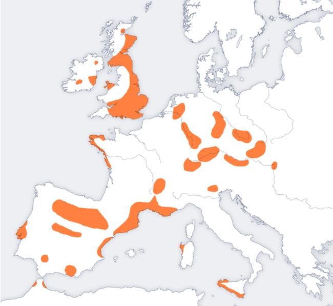
95 Figure 8 95