GPR Antennas Design and Experimental Evaluation

Transcription

1 Faculty of Electrical Engineering, Mathematics and Computer Science Microwave-transmission, Radar and Remote Sensing Technology (MTS Radar) group GPR Antennas Design and Experimental Evaluation H.G. Poley June 2010 Committee members: Prof.dr. A. Yarovoy Dr. D. Caratelli Dr.Ir. R.F. Remis Dr. M. Simeoni

2 Copyright 2010 by H.G. Poley All rights reserved. No part of the material protected by this copyright may be reproduced or utilized in any form or by any means, electronic or mechanical, including photocopying, recording or by any information storage and retrieval system, without permission of the author and Delft University of Technology. 2

3 Abstract In recent years the renewed interest in utility detection with GPR has led to the foundation of an EUfunded project called ORFEUS in which 9 partners including equipment developers, user organisations and academic institutions take part. One of the aims of this project is to improve the detection of utilities with GPR from the surface. Within this project IRCTR a department from the TU Delft has developed a resistively-loaded bow-tie antenna for the purpose of utility detection from the surface. This resistively-loaded bow-tie antenna was designed to operate in the frequency range from 100 MHz to 1 GHz, which is a typical operating range for utility detection with GPR. The challenge in this frequency range is that some objects will be in the near-field while other objects are located in the farfield. When using the antennas is pair configuration this will also hold for the transmitter and receiver antenna. As part of this thesis the performance of this resistively-loaded bow-tie antenna has been experimentally evaluated. Its performance is compared versus a Vivaldi antenna with known performance, its energy transfer to the soil has been evaluated for different heights above the soil. In pair configuration the mutual coupling of this antenna type is analyzed for different soil types, height above the surface and separations. In pair configuration this ORFEUS antenna system consisting of two of these resistively-loaded bowtie antennas has been compared versus a commercially available antenna system consisting of two dipole antennas. These antenna systems have been evaluated above three different test sites located in the Netherlands and France. The results of the experimental evaluation and the phenomena occurring in these measurements led to numerical analysis with a resistively-loaded printed dipole antenna to gain a better knowledge about the obtained results and utility detection in general. The resistively-loaded printed dipole antenna was designed to have a fractional bandwidth above 50% with a centre frequency around 400 MHz. This antenna was then analyzed in pair configuration to gain a better understanding of the mutual coupling for different situations. This was done by changing soil conditions, antenna height above soil, antenna separation etc. Further the detectability of pipes has been analyzed by changing the depth, radius, material and orientation of a buried pipe. The results of the experimental evaluation in terms of mutual coupling of the resistively-loaded bow-tie antennas indicated that when the antennas were approaching the soil, the proximity effect played a more important role allowing for direct coupling in the lower frequencies. However the antennas proved to be quite invariant to the soil conditions in terms of coupling. From the results it was seen that the resistively-loaded bow-tie antennas had a very large bandwidth at a -10 db return loss level, running from 70 MHz to 2.25 GHz which is larger than the desired frequency range from 100 MHz to 1 GHz. The good performance at especially the lower frequencies allows for the detection of buried utilities up to 2 meter. The numerical analysis with the resistively-loaded printed dipole antennas allowed for the design of an antenna that has a fractional bandwidth of 55% with a centre frequency of 363 MHz. Antenna efficiencies larger than 15% were achieved for the higher frequencies while at the lower frequencies the input impedance mismatch caused a low efficiency. The mutual coupling processes have been analyzed also indicating that the proximity effect plays a more important role when the antennas are approaching the soil. When analyzing the pipes for different conditions phenomena like creeping waves could be clearly seen in the analysis of a buried dielectric pipe. Also an inhomogeneous soil could mask the effect of a buried utility. 3

4 Acknowledgements As I did my thesis project within IRCTR of the TU Delft I would like to thank the people within IRCTR that were involved in this thesis project. They gave me advice and guidance when I was heading in the wrong direction, let me take part in the experimental evaluation of an antenna developed at IRCTR. Next to this I would like to thank the secretary of the Telecom department for the practical help they gave me when I needed something, like an access key, something printed, etc. I would also like to thank the people at the Electrotechnische Vereeniging (ETV) for the coffee, listening ear or distraction when needed. The same goes for the Dispuut TeleCommunicatie (DTC) as they made sure students and staff of the telecom department interacted more with each other resulting in a nice atmosphere to work in. All in all it has been a nice period in which I have learned a lot. 4

5 Table of Contents ABSTRACT...3 ACKNOWLEDGEMENTS...4 TABLE OF CONTENTS...5 LIST OF FIGURES...7 LIST OF TABLES...8 ABBREVIATIONS INTRODUCTION GROUND PENETRATING RADAR SCOPE OF THE THESIS OUTLINE OF THE THESIS ANTENNAS FOR GROUND PENETRATING RADAR BICONICAL AND BOW-TIE ANTENNA SPIRAL ANTENNA VIVALDI ANTENNA TEM HORN RESISTIVELY-LOADED ANTENNAS Resistively-loaded dipole antenna Resistively-loaded dipole antenna on a substrate Resistively-loaded bow-tie antenna on a substrate COMPARISON OF THE ANTENNA TYPES EXPERIMENTAL EVALUATION OF UWB ANTENNAS FOR THE GPR ORFEUS PROJECT EVALUATED ANTENNAS Resistively-loaded bow-tie antenna Vivaldi antenna Dipole antenna pair CIRCUITAL PERFORMANCE OF THE ORFEUS ANTENNA Comparison of the bow-tie antenna with a Vivaldi antenna Optimal height above sand Antenna footprint Mutual coupling above different soil types RADIATION PROPERTIES AND DIFFRACTION FROM BURIED TARGETS IN REALISTIC SCENARIOS B-scans at TNO B-scans carried out by IDS SUMMARY AND CONSEQUENCES OF THE EXPERIMENTAL EVALUATION DESIGN AND FULL-WAVE MODELLING OF A RESISTIVELY-LOADED PRINTED DIPOLE STRUCTURE PARAMETER ANALYSIS SINGLE ANTENNA Antenna efficiency Antenna footprint Electric field for different angles Time domain PAIR CONFIGURATION Separation Inhomogeneous soil Metal Pipe PVC Pipe CONCLUSIONS ON THE NUMERICAL ANALYSIS OF A RESISTIVELY-LOADED DIPOLE ANTENNA CONCLUSIONS AND RECOMMENDATIONS

6 5.1 EXPERIMENTAL VERIFICATION OF UWB ANTENNAS FOR THE GPR ORFEUS PROJECT INDIVIDUAL ANTENNA PERFORMANCE ANTENNAS IN PAIR CONFIGURATION RECOMMENDATIONS REFERENCES...62 APPENDIX A. EXPERIMENTAL EVALUATION OF THE ANTENNA SYB-SYSTEM OF THE ORFUS SURFACE GPR...64 B. EM CHARACTERIZATION OF RESISTIVELY-LOADED PRINTED DIPOLE ANTENNAS FOR GPR APPLICATION...70 C. SHIELDING...71 C.1 REFERENCES...72 D. NUMERICAL TECHNIQUES FOR SOLVING MAXWELL S EQUATIONS...78 D.1 FINITE DIFFERENCE TIME DOMAIN (FDTD) METHOD...78 D.1.1 Stability...79 D.1.2 Boundaries...80 D.1.3 Software...80 D.2 METHOD OF MOMENTS (MOM)...80 D.2.1 Accuracy...81 D.2.2 Software...82 D.3 CHOICE OF METHOD...82 D.4 REFERENCES

7 List of Figures FIGURE 1 PAPER ARTICLE ABOUT EXCAVATION WORKS IN THE MEKELPARK, TU DELFT (SOURCE: FIGURE 2 DUAL CONFIGURATION FOR DETERMINING THE LOCATION OF OBJECTS...11 FIGURE 3 EXAMPLE OF A B-SCAN. ON THE HORIZONTAL AXIS THE POSITION OF THE ANTENNA MEASUREMENTS IS SHOWN AND ON THE VERTICAL AXIS THE DEPTH OR PROPAGATION TIME. THE YELLOW/RED CIRCLE INDICATES THE PRESENCE OF ONE OBJECT FIGURE 4 A BICONICAL ANTENNA (LEFT) AND A BOW-TIE ANTENNA (RIGHT)...15 FIGURE 5 EXAMPLE OF A SPIRAL ANTENNA ON A SUBSTRATE [9] FIGURE 6 EXAMPLE OF A VIVALDI ANTENNA, ETSA_A3 [11] FIGURE 7 TOP VIEW OF THE DIPOLE ANTENNA ON A SUBSTRATE FIGURE 8 RESISTIVELY-LOADED BOW-TIE ANTENNA [9]...19 FIGURE 9 - RESISTIVELY-LOADED BOW-TIE ANTENNAS AS USED IN THE ORFEUS ANTENNA SUB-SYSTEM FIGURE 10 VIVALDI ANTENNA AS USED IN THE EXPERIMENTAL EVALUATION...23 FIGURE 11 IDS ANTENNA SYSTEM USED FOR COMPARISON WITH THE ORFEUS IN THE EXPERIMENTAL EVALUATION...23 FIGURE 12 MEASUREMENT SETUP FOR MEASURING THE S 11 AND S 21 -PARAMETERS OF THE RESISTIVELY LOADED BOW-TIE WITH A LOOP ANTENNA. THIS SETUP HAS ALSO BEEN USED FOR DETERMINING THE ANTENNA FOOTPRINT FIGURE 13 MEASUREMENT SETUP USED TO CHECK THE ANTENNA PERFORMANCE WITH DIFFERENT CAVITY CONFIGURATIONS...24 FIGURE 14 S 21 -PARAMETERS FOR A LOOP ANTENNA WITH A BOW-TIE OR A VIVALDI ANTENNA AT A DISTANCE OF 1 METER FIGURE 15 TIME DOMAIN SIGNAL FOR THE BOW-TIE ANTENNA AND A VIVALDI ANTENNA WHEN PLACED 4 CM ABOVE THE SANDY SOIL SURFACE FOR A PERIOD OF 10 NS...25 FIGURE 16 RETURN LOSS FOR DIFFERENT ELEVATIONS ABOVE DRY SANDY SOIL...26 FIGURE 17 S 21 -PARAMETERS FOR A BOW-TIE ANTENNA THAT IS PLACED AT DIFFERENT ELEVATIONS ABOVE A SANDY SOIL SURFACE. THE LOOP ANTENNA IS PLACED 17 CM BELOW THE SAND SURFACE FIGURE 18 ANTENNA ORIENTATION FOR MEASURING THE COUPLING IN THE H-PLANE (LEFT) AND IN THE E- PLANE (RIGHT) FIGURE 19 COUPLING BETWEEN TWO RESISTIVELY LOADED BOW-TIE ANTENNAS FOR THE E-PLANE AND THE H- PLANE WHEN HE ANTENNAS ARE PLACED AT A HEIGHT OF 4 CM AND SEPARATED FROM EACH OTHER BY 1 CM FIGURE 20 NORMALIZED FOOTPRINTS OF THE BOW-TIE ANTENNA IN THE FREQUENCY RANGE MHZ FIGURE 21 THE SIX TEST LANES LOCATED AT THE TNO TEST SITE WITH DESCRIPTION OF THE SOIL TYPES [18]. 29 FIGURE 22 MUTUAL COUPLING IN FREQUENCY-DOMAIN FOR FOUR DIFFERENT CONFIGURATIONS REGARDING HEIGHT AND SEPARATION ABOVE DIFFERENT SOIL TYPES...30 FIGURE 23 MUTUAL COUPLING IN TIME-DOMAIN FOR THE ORFEUS ANTENNAS GIVEN FOR AN ANTENNA HEIGHT OF 4 CM AND SEPARATION OF 1 CM (A) AND 10 CM (B) AND AN ANTENNA HEIGHT OF 0 CM AND ANTENNA SEPARATION OF 1 CM (C) AND 10 CM (D). WATCH THE TIME-SCALE FOR (C) AND (D) FIGURE 24 S-PARAMETERS OF THE IDS ANTENNA SYSTEM TAKEN ABOVE SAND WITH A RELATIVE PERMITTIVITY OF FIGURE 25 LOCATIONS OF THE BURIED TARGETS IN THE SANDPIT COVERED BY THE SCANNER CONSTRUCTION..33 FIGURE 26 B-SCANS OF THE THREE PIPES WITH THE RESISTIVELY-LOADED BOW-TIE ANTENNAS (A) AND DIPOLE ANTENNAS (B) AND THE B-SCANS OF THE SPHERE WITH THE RESISTIVELY-LOADED BOW-TIE ANTENNAS (C) AND DIPOLE ANTENNAS (D) FIGURE 27 B-SCANS AT GAZ DE FRANCE IN PARIS WITH THE ORFEUS ANTENNA SYSTEM (A) AND THE IDS ANTENNA SYSTEM (B) WITH OBJECTS AT LARGER DEPTHS FIGURE 28 B-SCAN AT VILLEFRANCHE WITH THE ORFEUS ANTENNA SYSTEM, SHOWING THE CAPABILITIES TO DETECT AN OBJECT AT A DEPTH OF ALMOST 2 METER AS SHOWN IN THE YELLOW RECTANGLE FIGURE 29 IMAGE OF THE MODEL BUILD IN CST...37 FIGURE 30 GAUSSIAN PULSE THAT IS FED TO THE ANTENNA...37 FIGURE 31 PARAMETER ANALYSIS FOR DIFFERENT VALUES OF N AND σ 0, HERE THE MINIMUM VALUE OF S 11, THE CENTRE FREQUENCY AND THE ABSOLUTE AND FRACTIONAL BANDWIDTH ARE GIVEN...38 FIGURE 32 EXAMPLE OF A SURFACE IN THE X-PLANE...40 FIGURE 33 INPUT EFFICIENCY OF THE ANTENNA FOR THE FREQUENCY RANGE OF INTEREST

8 FIGURE 34 FOOTPRINTS OF THE ANTENNA FOR DIFFERENT FREQUENCIES RANGING FROM 100 MHZ TILL 1 GHZ AT THE TOP OF THE SOIL SURFACE FIGURE 35 FOOTPRINTS OF THE ANTENNA AT THE FOR THE POLAR AND CROSS-POLAR COMPONENT AT THE TOP OF THE SURFACE (Z=0 CM) AND 10 CM BELOW THE SURFACE (Z=-10 CM) AT 400 MHZ...43 FIGURE 36 ANTENNA FOOTPRINT AT 400 MHZ WITH Z = 0 CM FOR BASIC SOIL, DRY CLAY AND WET CLAY...44 FIGURE 37 NEAR-FIELD RADIATION PATTERN IN THE XZ-PLANE FOR 100 MHZ, 500 MHZ AND 1 GHZ. ZERO DEGREES CORRESPOND TO THE POSITIVE Z-DIRECTION, WHILE 90 DEGREES IS THE POSITIVE X-DIRECTION...45 FIGURE 38 CURRENT (A) IN THE ANTENNA GIVEN FOR TIME AND POSITION FIGURE 39 S 11 -PARAMETERS FOR DIFFERENT HEIGHTS AND DIFFERENT SEPARATIONS IN THE RANGE FROM 55 MM TILL 550 MM...47 FIGURE 40 S 21 -PARAMETERS FOR DIFFERENT HEIGHTS AND DIFFERENT SEPARATIONS IN THE RANGE OF 55 MM TILL 550 MM...47 FIGURE 41 TIME-DOMAIN SIGNAL AT THE TRANSMITTER ANTENNA AND AT THE RECEIVER ANTENNA FOR AN ANTENNA SEPARATION OF 165 MM AND AT A HEIGHT OF 3 CM ABOVE THE SOIL...48 FIGURE 42 BOTTOM VIEW OF ALL THE OBJECTS IN THE INHOMOGENEOUS SOIL IN THE XY-PLANE...49 FIGURE 43 S-PARAMETERS FOR HOMOGENEOUS AND INHOMOGENEOUS SOIL FIGURE 44 POSITION OF THE ANTENNAS ON THE X-AXIS FIGURE 45 S-PARAMETERS FOR DIFFERENT DEPTHS OF A METAL PIPE. THE ANTENNAS ARE PLACED 165 MM APART FIGURE 46 TIME-DOMAIN DIFFRACTED SIGNAL DUE TO A METAL PIPE FOR DIFFERENT DEPTHS...51 FIGURE 47 S 21 -PARAMETER FOR THE DIFFERENT LOCATIONS OF THE PIPE SHIFTING FROM X = -200 MM TO X = 200 MM FIGURE 48 INTENSITY PLOT FOR RECEIVED SIGNAL WITH BACKGROUND SUBTRACTION...52 FIGURE 49 TOP VIEW OF THE TWO ANTENNAS AND A PIPE PLACED UNDER DIFFERENT ANGLES...53 FIGURE 50 - S 21 -PARAMETERS FOR DIFFERENT ANGLES WITH REGARD TO THE ANTENNA INCLUDING A BURIED METAL PIPE AT 30 CM DEPTH FIGURE 51 TIME-DOMAIN DIFFRACTED SIGNAL AT RECEIVER AND TRANSMITTER ANTENNA FOR A BURIED METAL PIPE PLACED UNDER DIFFERENT ANGLES AT 30 CM DEPTH, WHERE THE NUMERICAL ERROR IS VISIBLE BELOW 7 NS DUE TO DIFFERENT MESHING OF THE ENVIRONMENT...54 FIGURE 52 S 21 -PARAMETERS FOR DIFFERENT ANGLES OF A METAL PIPE BURIED AT A 10 CM DEPTH WITH REGARD TO THE ANTENNA FIGURE 53 DIFFRACTED SIGNAL DUE TO A BURIED METAL PIPE AT A DEPTH OF 80 CM, WHERE THE MESH INFLUENCE IS REMOVED AS IT ARRIVES AT AN EARLIER TIME-INSTANCE FIGURE 54 VOLTAGE INTENSITY FOR DIFFERENT RADII OF THE PIPE GIVEN OVER TIME...55 FIGURE 55 - VOLTAGE AT RX MINUS SIGNAL WITHOUT PIPE...56 FIGURE 56 INTENSITY PLOTS FOR DIFFERENT DIAMETERS OF A PVC PIPE GIVEN OVER TIME, SHOWING THE CREEPING WAVES EFFECT FIGURE 57 COUPLING FOR DIFFERENT ANGLES OF A BURIED PVC PIPE FIGURE 58 DIFFRACTED SIGNAL DUE TO A BURIED PVC PIPE WITH A 6 CM DIAMETER AT A DEPTH OF 80 CM...58 List of Tables TABLE 1 ANTENNA ELEMENTS ANT THEIR PERFORMANCE AND CHARACTERIZATIONS [13]...20 TABLE 2 CHARACTERISTIC OF DIFFERENT ANTENNA TYPES THAT ARE PLACED ON A SUBSTRATE OR DIELECTRICALLY FILLED (VIVALDI)...20 TABLE 3 THE FOUR CONFIGURATIONS USED FOR THE A-SCANS SPECIFYING HEIGHT ABOVE THE SURFACE AND THE SEPARATION BETWEEN THE TWO ANTENNAS...29 TABLE 4 LOCATION AND DIMENSIONS OF THE METAL OBJECTS BURIED IN THE GROUND AT THE TNO SANDPIT. 32 TABLE 5 ANTENNA PARAMETERS...36 TABLE 6 RESISTOR VALUES FOR N = 12 AND σ 0 = 113 S / m GIVEN FOR ALL THE TRANSISTORS IN ONE ANTENNA FLARE TABLE 7 RADIATION EFFICIENCY, REFLECTION EFFICIENCY AND THE ANTENNA EFFICIENCY GIVEN FOR DIFFERENT FREQUENCIES...41 TABLE 8 CHARACTERISTICS OF THREE DIFFERENT SOIL TYPES USED FOR DETERMINING THE ANTENNA FOOTPRINT

9 Abbreviations ABC Absorbing Boundary Conditions BW Bandwidth EMI Electromagnetic Interference FBW Fractional Bandwidth FDTD Finite Difference Time Domain FEM Finite Element Method GPR Ground Penetrating Radar IFFT Inverse Fast Fourier Transform IRCTR International Research Centre for Telecommunications and Radar MoM Method of Moments ORFEUS Optimised Radar to Find Every Utility in the Street PEC Perfect Electric Conductor PML Perfectly Matched Layer PVC Polyvinylchloride RAM Radar Absorbing Material UWB Ultra Wideband VNA Vector Network Analyzer VSWR Voltage Standing Wave Ratio 9

10 1 Introduction This thesis research has been a consequence of the renewed interest in utility detection. For this purpose an EU-funded project named ORFEUS (Optimised Radar to Find Every Utility in the Street) was set up with a focus on utility detection with Ground Penetrating Radar (GPR) [1]. The advantage of GPR above many other methods is that it works in a non-evasive way. This means that to detect the buried pipes and cables no holes or trenches have to be dug. Simply by scanning on the surface an indication of what is below the surface will appear. The effectiveness of such an approach is clearly demonstrated by the following article found in the TU Delft newspaper Delta in Figure 1. Spending an entire day digging trenches is a lot more labour-intensive than operating a scanning device on the surface. Translation: Patrick Boucquez (50 next month) is a professional digger. His employer BAM has lent him to region West. Today, he already dug 7 trenches in search for cast iron water pipes, which should still be there. These pipes need to be removed due to the construction of a new tram line. However, he has not found any. The drawings stating the location of the pipes are incorrect due to all the excavation works in the Mekelpark. Today, his efforts were in vain Figure 1 Paper article about excavation works in the Mekelpark, TU Delft (Source: From this article it is also clear that utilities buried in the past are located on paper, but due to ground movement of other excavation works utility pipes and cables can be moved. Further, there can be a difference between the location stated on paper and where the utilities are actually buried due to crossings with other utilities or corners, etc. 10

11 Another example of the impact of not exactly knowing the location of utilities is when an excavator accidently hits a buried power line or water supply pipe. Thousands of people will suffer from a small error made by one person who was badly informed. Repairing such mistakes is costly and these costs will usually be for the company performing the construction works. Therefore such companies have an interest in reducing the number of incidents by finding the exact location of these utilities themselves. 1.1 Ground Penetrating Radar As said before, GPR stands for Ground Penetrating Radar, which allows scanning the soil in a nonevasive way. In GPR electromagnetic signals are transmitted into the ground and by analyzing and post-processing the received signals an insight can be obtained in objects present in the soil. Just like with normal radar for detection of ships and aircrafts analysis of the received signal gives the distance to objects. These objects can be a range of things depending on the applications. Possible applications are landmine detection, archaeological surveys, road or rail inspections and of course the before mentioned utility detection. For transmitting these electromagnetic signals into the ground probes can be placed in the ground or an antenna can be placed on top of the surface. Placing the antennas above ground makes operation of the radar system easier as it can be easily moved, but an extra challenge arises for this problem as the soil will introduce an extra reflection. When the antenna is placed above ground the propagation time from the first reflection is usually short than the signal duration hence a dual antenna system is chosen where one antenna functions as a transmitter and another antenna as a receiver. Transmitter Receiver Object Figure 2 Dual configuration for determining the location of objects. In time-domain information about the distance can then be obtained by analyzing the propagation time between the transmitter and the receiver as seen in Figure 2. To obtain the distance of the object with regard to the antennas the propagation speed has to be known of the soil, which is determined by the electrical properties of the soil via equation (1.1). Where ε m is the permittivity of the material in F / m and μ m the permeability in H / m. The propagation speed can also be defined via the speed of light ( c ) and the relative permittivity ε r as seen in equation (1.2) 1 v = (1.1) ε μ c v = (1.2) ε r One such a sample taken to measure the distance to objects present in the soil is called an A-scan. When a series of A-scans is performed the result is called a B-scan and represents a cross-section of the soil with the range to objects present in the soil from the top of the surface. The presence of an object is then shown by an arc as can be more clearly seen in Figure 3, where one object is marked by a yellow/red circle. The shape of the arc is determined by the propagation speed and the top of the arc indicates the real position of the object. In Figure 2 the transition between soil and air is also shown. Since the relative permittivity of the soil is higher than that of the air there will be a mismatch between these media. The height of the antenna above the soil is partly responsible for the amount of mismatch that will occur. The lower the antennas m m 11

12 height is above the surface of the soil the more the soil will be part of the antenna system resulting in a lower mismatch and a higher amount of energy transmitted in the soil. However in GPR the devices that are handled do not stay at a fixed height above the surface, due to an uneven surface or due to handling during operation. Another important factor with GPR is the range-resolution. A lower frequency has a larger penetration depth but a lower resolution; a higher frequency gives a better resolution but comes at the cost of range. To overcome this problem in GPR often Ultra-Wideband (UWB)-signals are used, where a frequency range of a decade or larger is used. The frequency range is then dependent on the depth of the objects, their size and the accuracy needed. Figure 3 Example of a B-scan. On the horizontal axis the position of the antenna measurements is shown and on the vertical axis the depth or propagation time. The yellow/red circle indicates the presence of one object. 1.2 Scope of the thesis The EU-funded project named ORFEUS was set up by nine partners including the TU Delft [2]. These partners consist of equipment developers, user organisations and academic institutions. One of the aims of this project is: To improve the performance of GPR deployed on the surface to provide underground maps. In order to realize this aim it has been divided in several sub tasks. Two sub tasks related to this thesis are a better understanding of the soil that needs to be realized and an enhanced antenna needs to be developed which if possible is adaptable to the soil conditions. Within this project IRCTR has developed a resistively-loaded bow-tie antenna, which has been designed to operate in the frequency range from 100 MHz till 1 GHz. The challenges are that for the lower frequencies most objects will be in the near-field of the antenna and for higher frequencies these will be in the far-field of the antenna. As part of this thesis experimental evaluation has been carried out with this resistively-loaded bow-tie antenna. Its performance has been compared versus other antenna types. Mutual coupling was analyzed for different separations and heights above different soil types as the loading increases when the antennas approach the soil. Further a system containing two of these resistively-loaded bow-tie antennas was compared versus a commercially available antenna system regarding the detectability of buried utilities. 12

13 One of the results was the occurrence of long-in-time coupling, while coupling levels at all frequencies stayed below -30 db. To get a better understanding of the phenomena occurring in the mutual coupling processes and sub-surface scattering different configurations were numerically analyzed with a resistively-loaded dipole pair. This is done by characterizing a resistively-loaded dipole antenna which will be designed according to the following specifications: The centre frequency should be around 400 MHz. The fractional bandwidth should be larger than 50% at a -10 db return loss level The coupling level in pair configuration should be below -20 db Numerical analysis will then be carried out for different situations to gain a better knowledge of the time-domain behaviour of the diffracted radio signal from buried pipes. This will be done by changing the depths of the pipes, their location with regard to the antennas and their orientation. As a result of the experimental evaluation of the ORFEUS antennas and numerical analysis of a resistively-loaded printed dipole two papers have been submitted and have been accepted at the XIII International Conference on Ground Penetrating Radar, which will be held from 21 June till 25 June in Lecce, Italy. The first paper about the experimental evaluation of the ORFEUS antenna system is titled Experimental Evaluation of the Antenna Sub-system of the ORFEUS Surface GPR and can be found in Appendix A, the second paper is titled EM characterization of Resistively Loaded Printed Dipole Antennas for GPR Applications and can be found in Appendix B. 1.3 Outline of the thesis Different antenna types for utility detecting with GPR are discussed and compared in chapter 2. These antenna types are compared and analyzed on several aspects like size, efficiency, footprint, polarization, etc. Chapter 3 will cover the experimental verification performed on the resistively-loaded bow-tie antennas developed by IRCTR for the ORFEUS project. This antenna is compared versus a Vivaldi antenna in single antenna performance, its footprint is analyzed above a sand pit and mutual coupling processes are analyzed for different situations. Further the ORFEUS antenna is compared versus a commercially available antenna system to analyze the detection performance of buried utilities of this antenna system. In Chapter 4 a numerical investigation of mutual coupling processes has been carried out. This is done by designing and optimizing a resistively-loaded printed dipole antenna. This antenna system will then be used in pair configuration to analyze the processes taken place in utility detection with UWB GPR antennas. Situations were a pipe is located beneath the surface of the soil are then analyzed for different configurations were the depth of the pipe, its location and orientation with respect to the antennas are changed. Finally, conclusions from the experimental evaluation and numerical investigation on the mutual coupling processes are given in Chapter 5. Also recommendations for further investigations will be given. 13

14 2 Antennas for Ground Penetrating Radar For detecting objects in the ground with GPR different antenna types can be used. The best suitable antenna type is determined by the application as the objects that need to be detected and the environment determine the different parameters for an antenna. In this thesis report the purpose is to detect pipes and cables from the surface and therefore this chapter will cover the discussion and analysis of different antenna types; there suitability for pipe and cable detection will be analyzed on several aspects which will be explained below. First of all the physical dimensions and weight of an antenna are of importance for pipe and cable detection the antennas. A detection system will be used at a construction site and the scanning should be easy to perform, preferably by one person. The second aspect is the range-resolution. The detection range is depended on the used frequencies as longer radio waves are less distorted by attenuation in the ground. On the other side the resolution is also dependent on the used frequencies as for higher frequencies the resolution increases. To overcome this Ultra-Wideband (UWB) can be used as it provides good-range resolution. Desirable is to have a decade for bandwidth, like the 100 MHz till 1 GHz as for the ORFEUS antenna, which provides a good range-resolution for pipe and cable detection. Since with increasing depth the size of the buried pipes and cables also increases the loss of resolution does not matter that much [3], [4]. The third aspect is the efficiency of the antenna system. This is determined by the radiation efficiency of the antenna for all frequencies. Also matching to the ground is of importance as the antennas will be placed above the surface, the soil is also part of the antenna system. One way to do this is to build the antenna on a substrate or use dielectric filling with a certain relative electrical permittivity ε r which has a value close to that of the soil. The effect of this is a reduction of reflections that happen at the air-ground interface, resulting in a lower return loss. Further, all energy should be directed to the ground as energy directed upwards is of no use for detecting buried objects and will only cause electromagnetic interference (EMI) with other objects in the surroundings. Placing an antenna on a substrate also has the advantage that the radiation is focussed mostly on the side of the substrate. The polarization of the antennas is another important aspect of for pipe detection. When the antennas are rotated with regard to the pipes a sinusoidal behaviour can be seen in the amplitude of the received signal with maxima when the pipes and antennas are parallel and minima when the pipes and antennas are perpendicular. To overcome this problem different polarisation configurations can be used or antenna behaviour itself can overcome this. On the other hand most pipes and cables are buried in line with the road and hence most of the times scanning in one direction will work, however the danger lies in not detecting an pipe in an unexpected direction as it will be orthogonal to the linear antennas. The last aspect is the antenna footprint as in general the antenna footprint should have a shape similar to the objects that need to be detected. In the case of pipes and cables this implies that the footprints should have an elongated shape. But this is only the case when the antennas and pipes are aligned, when this is not the case the detection performance will drastically reduce. 2.1 Biconical and bow-tie antenna The first example of an UWB antenna is the biconical antenna as shown in Figure 4 on the left which as the name suggests consists of two cones. Its wideband character is determined by the size of the cones, the length determines the centre frequency and the diameter at the ends the wideband behaviour. Its behaviour depends on the size of antenna with regard to the frequency, when the aperture is less than 0.6 times the wavelength the antenna can be regarded as a dipole with conical arms and when the antenna is larger than 0.6 times the wavelength it can be considered as a horn antenna [5]. For 100 MHz this transition is at 1.8 m and at 1 GHz this would occur at 18 cm, hence for a wideband spectrum the antenna behaviour will have elements of both. Its radiation pattern is like a dipole rotationally symmetrically shaped around the centre of the antenna. Further the transmitted beamwidth depends on the wavelength and the vertical aperture of the antenna as seen in equation (2.1), where D is the vertical aperture and λ the wavelength. 65λ Beamwidth (elevation) = degrees (2.1) D 14

15 A disadvantage of this antenna type is its size and weight, especially when used for lower frequencies. This problem can be partly overcome by constructing the biconical antenna from a wireframe, but this will change antenna characteristics and slightly increase ringing effects. Another option is to flatten the biconical antenna which is known as the bow-tie antenna as shown in Figure 4 on the right. By almost eliminating one dimension the weight is drastically reduced, also the size is reduced in one dimension. This adaption of the antenna will also change the behaviour of the antenna; the directivity will be more focussed to the top and bottom of the antenna. But for GPR this is an advantage. Like the wired biconical antenna the bow-tie shows fluctuation of the resistance and reactance over the frequency band caused by ringing effects [6]. The advantage of the bow-tie above a wired biconical antenna is that it can be constructed on a substrate and hence can be better matched to the soil. These antennas show linear polarization and their footprints will have an elongated shape, but can become more elliptical depending on the width of the flares. Figure 4 A Biconical antenna (left) and a bow-tie antenna (right). 2.2 Spiral antenna The spiral antenna is an antenna consisting out of spiral(s) and an example of a dual spiral antenna can be seen in Figure 5. The lowest operating frequency is determined by the length of the arms as this is equivalent to the maximum wavelength [7]. However, for a more equal performance over the frequency band it is recommend that the spiralling flares become wider towards the ends [8]. Since the spiral antenna is folded the diameter of the antenna is smaller then the length of a spiral, reducing the size of the total antenna. Figure 5 Example of a spiral antenna on a substrate [9]. This antenna type is characterized by the fact that it makes a distinction between frequencies in timedomain as higher frequencies travel a shorter distance in the antenna before the waves are radiated and hence the lower frequencies will radiate at a later time instance. The spiral antenna can also be constructed on a substrate allowing the antenna to be closer matched to the soil and the direction of radiation to be mostly focussed into the ground. The big advantage of the spiral antenna is the circular polarization making it possible to detect buried pipes under all angles. The footprint however is more circular making it less suitable for detecting long objects like pipes as the maximum amplitude of the reflection is reduced. 15

16 2.3 Vivaldi antenna A Vivaldi antenna is a special tapered slot antenna with a planar structure [10]. It consists of a microstrip feed and one or two outer metal planes that act as a ground plane separated by a dielectric. An example can be seen in Figure 6, where there are two ground planes and extra foam is added for separation, which is not a necessary feature of the Vivaldi antenna. The travelling wave excitation of this antenna type performs very well over the entire designed frequency band and does hardly suffer from ringing effects. The distance between the flares at the end of the antenna determines the minimum frequency, which corresponds to half the wavelength. For a good performance at 100 MHz the antenna would measure λ /2 = c/2f = 3e8/2 100e6= 1.5 m. This distance can be reduced by increasing the relative permittivity of the dielectric of the antenna. When increasing the relative permittivity to er 4 the size of the antenna still measures 75cm. The length of the antenna determines the antenna gain and a longer antenna will result in a better gain. In general the antenna length is the same or larger than the width, resulting in a large but flat antenna. The substrate used in the antenna also makes it possible to match the Vivaldi antenna better to the soil. The antenna polarization of this antenna type is also linear and the footprint shows an elongated shape. 2.4 TEM Horn Figure 6 Example of a Vivaldi antenna, ETSA_A3 [11]. The TEM horn is the most common type of horn antenna and is a so-called waveguide antenna. Its main principle of operation is two parallel plate lines that towards the end of the antenna increase in separation. For the lowest mode of operation the maximum wavelength that can be transmitted from the antenna is determined by the separation at the end of the antenna. Hence the same problem arises as with the Vivaldi antenna. For a minimum frequency of 100 MHz the size should be 1.5 m, unless the separation between the plates is filled with a dielectric. To reduce ringing effects in the antenna the transition of the feed to freespace or the electrical permittivity close to that of the soil must be smooth in order to suppress reflections. Since the energy is transmitted via the horn the dimensions of the horn can steer the energy and a focussed beam can be formed to emit the waves. The footprint therefore is dependent on the shape of the horn. This antenna type is also characterized by linear polarization and the footprint is determined by the antenna shape at the end of the flares. 2.5 Resistively-loaded antennas Another way to increase the bandwidth of an antenna is to use resistive loading. For a dipole this means that towards the ends of the antenna the impedance increases. However the use of resistors will result in extra losses in the antenna, reducing its efficiency. For better matching to the soil the 16

17 impedance of the antenna should be closely matched to that of the soil to reduce reflections at the airground interface of the antenna. The relative small size of this dipole also makes it possible to be used in different configurations to cover different polarizations Resistively-loaded dipole antenna The loading profile of such a resistively-loaded dipole is usually exponential and increases towards the antenna ends. One example of such a loading profile is the Wu-King loading profile [12]. This profile is described by equation (2.1). η0ψ 1 Z( z) = (2.2) 8π h z 1 h μ0 In this equation η0 = is the intrinsic impedance, h is the length of a dipole arm, z is the ε 0 position on the dipole arm and Ψ is a dimensionless parameter described by the electrical dimension of the antenna, usually the DC-component Ψ is used. 0 The first term of equation (2.2) states the electrical dimensions of the antenna and the total loading while the second term determines the loading profile along the antenna flares. Thus at the end of the dipole the loading is approaching infinite and at the centre the loading corresponds to the first term of this equation. The input impedance of the antenna can be approximated by: Zin 60Ψ 0, (2.3) and hence a value of Ψ 0 = 5 gives an approximate input impedance of Zin 300Ω. When placing the antenna above ground the loading will slightly increase and hence a value of Ψ 0 = 4.5 is more suitable. The efficiency of this antenna will be better at the non-resonant frequencies of a dipole, but this comes at the costs of worse performance at the resonance frequencies. As known a dipole antenna has linear polarization and this is also the case for a resistively-loaded dipole. The footprint will be elongated just like a normal dipole antenna Resistively-loaded dipole antenna on a substrate The resistively-loaded dipole antenna can also be created on a substrate, which makes it possible to match the antenna better to the soil. The disadvantage is that the antenna loading increases due to the capacitive loading caused by the substrate giving the antenna high input impedance which means it will be more difficult to match the antennas to the feeding cable. When implementing a resistively-loaded dipole on a substrate it is easier to discretize the loading of the antenna. An example of such an implementation of the resistively-loaded dipole is given in Figure 7. The antenna consists of two slotted flares, where a flare is divided into N + 1 segments which are equally spaced from each other by a distance S. These flares are made out of copper with dimensions w a and l a and are then placed on a substrate with dimensions w s by l s. The two flares are separated by a feed gap ( δ a ) and contain N resistors. 17

18 Figure 7 Top view of the dipole antenna on a substrate. The electrical properties of the antenna are described by the following parameters. First the parameter Ω 0 gives the electrical conductivity in S/m at the centre of the antenna and for the rest of the antenna the electrical conductivity is then given by equation (2.4) where y is the position on the antenna and l a the length of the dipole arm. 2 m is the cross- 2y σ y =Ω0 1 la The resistance at a certain location is then given by equation (2.5), where sectional area of the radiating flares. A a in (2.4) 2y ln 1 l a la Rf ( y) = (2.5) 2Aa Ω0 Since the antenna is divided into equally-spaced slots the step size is determined by the number of segments ( N ), and hence the step size ( Δ y) is given by: Δ y =. (2.6) 2( N + 1) From all formulas above the value of a resistor at a certain slot can be determined. A resistor at a certain location is also dependent on the values of the transistor placed before it. This results in the following formula for a resistor at slot n : 2nΔy 2( n 1) Δy ln 1 la ln 1 l la la Rn = Rf ( nδy) Rf (( n 1) Δ y) = 2AaΩ0 2AaΩ0 l a la 2( n 1) Δy = ln, where n= 1, 2,..., N, 2AaΩ0 la 2( n) Δy assuming that the dipole arms itself consists of perfectly electric conducting material. The antenna efficiency will be a little lower than that of a resistively-loaded antenna that is not build on a substrate due to the loading of the substrate and possible losses in the substrate. However the energy will be directed more to the soil due to the substrate compensating for this loss. l a a (2.7) 18

19 The polarization of this resistively-loaded dipole on substrate will be linear and the footprint will have elongated shape like the normal dipole. Its pattern in the E-plane however will be focussed to the top and bottom due to the substrate Resistively-loaded bow-tie antenna on a substrate Like a dipole antenna a bow-tie antenna can also be resistively-loaded. This will allow for a wideband character not only caused by its dimensions but also by the resistive loading. An example of a resistively-loaded bow-tie is displayed in Figure 8. Figure 8 Resistively-loaded bow-tie antenna [9]. The loading profile can be described by different functions and would depend on the application. In the case of the antenna displayed in Figure 8 the electrical conductivity σ is described by equation (2.8). In this equation ρ is the radial distance from the centre of the antenna, s is the flare length and σ min = σ f () s the conductivity value at the antenna end. Ω 0 is the resistance parameter determining the total loading of the antenna. σ min ρ 1+ Ω0 s σ f ( ρ) =Ω 0 (2.8) ρ s The antenna efficiency will be lower than that of the normal bow-tie antenna due to losses in the resistors, but the wideband behaviour will be better. The polarization and footprint will be the same as the non-loaded bow-tie antenna, meaning linear polarization and an elliptical footprint. 2.6 Comparison of the antenna types In this chapter different antenna types have been analyzed and their advantages and disadvantages have been discussed. A number of antenna parameters will be compared in this section. The first antenna parameters to be compared are the bandwidth, radiation pattern and polarization as seen in Table 1. From this table it can be seen that all antennas should be able to handle 100 MHz, but the antenna size need for this operation is not shown. Loading the antennas with resistors or filling with a dielectric material will reduce the size of the antenna. It can be seen that the only antenna suitable to handle several polarization types is the spiral antenna. Hence, this antenna type will perform better when pipes are buried under an angle in comparison with the other antennas that show linear polarization. What also can be noticed is that the dipole and the biconical antennas both have an omni-directional pattern in the H-field. The other antennas have a focused beam which allows for a more efficient transfer of energy in the soil. f 19

20 For the purpose of utility detection from the surface it is in general better for an antenna type to be constructed on a substrate or by dielectric filling so the antenna will be better matched to the soil and the reflection at the air-ground interface will be reduced, resulting in a lower return loss. The Vivaldi and TEM horn antenna will however have a larger height than an antenna printed on a substrate would have, which will be flat structures. Antenna type Dipole Bicone TEM Horn Vivaldi Spiral Upper frequency (GHz) Lower frequency (MHZ) Maximum Bandwidth- VSWR Maximum bandwidthpattern H-field pattern :1 5:1 12:1 10:1 40:1 6:1 5:1 12:1 3:1 40:1 Beam Beam Beam E-field pattern Cosine Beam Beam Beam Beam polarization linear linear linear Linear Circular Dispersion No No No Yes Yes Omnidirectional Omnidirectional Table 1 Antenna elements ant their performance and characterizations [13]. Some of the more important properties of antennas constructed on a substrate or that have an dielectric filling (Vivaldi) have been put in Table 2 for comparison. This allows for a better overview and selection of an antenna type for pipe and cable detection. Antenna Size Weight Wideband Efficiency Polarization Footprint performance Vivaldi High Average Good High Linear Elongated and flat Spiral Relative Average Fairly good High Circular Circular large Resistivelyloaded Small, Low Average Average Linear Elongated dipole narrow Resistivelyloaded bowtie Average Average Good Average Linear Elliptical Table 2 Characteristic of different antenna types that are placed on a substrate or dielectrically filled (Vivaldi). The best antenna when looking at size and weight would be the loaded dipole antenna as they are narrow, the Vivaldi antenna is also narrow but has a large height and the other antennas will be disc shaped or rectangular. The wideband performance of the Vivaldi antenna will be best together with the resistively-loaded bow-tie. The loaded antennas show a lower efficiency due to the losses in the resistors but this will come with an improved wideband performance. The Vivaldi antenna will have a high efficiency due to the low ringing effects in the antenna. The spiral antenna will also have a high efficiency for a wide frequency range, but like the Vivaldi the performance at lower frequencies might be a problem. The only antenna that has circular polarization is the spiral antenna giving a strong reflection for all angles of a buried pipe or cable. The other antennas will perform better when the pipes and cables are aligned with the antennas. When looking at the footprint an elongated footprint will give a strong reflection when the buried pipes and cables are aligned along the footprint as a greater area is radiated resulting in more energy 20

21 reflected back. When not aligned properly this area will reduce, also reducing the amount of energy reflected back while for a circular footprint this does not matter. With the weight and size being of big importance the antennas constructed on a substrate would be a good option as they are flat and can have dimensions below 50 cm for the lower frequency range and have a low height. Also the footprints of the dipole and bow-tie antennas on substrate are in their favour. The resistive loading allows for an even larger wideband character however at the cost of extra introduced losses. 21

22 3 Experimental evaluation of UWB antennas for the GPR ORFEUS project This chapter is focussed on the experimental evaluation of a resistively-loaded bow-tie antenna that was developed at IRCTR as part of the ORFEUS project [14]. Its performance is compared versus a Vivaldi antenna to gain a better insight in the circuital behaviour of this antenna. The ORFEUS system consisting of two of these resistively-loaded bow-tie antennas is compared versus a commercially available antenna system made for utility detection. The different antennas used in the experimental evaluation will be discussed in the first section. The second section is about the circuital behaviour of the radiating structures, comparing the ORFEUS antenna versus a Vivaldi antenna as well as the analysis of experimental results to gain a better understanding of the performance of the ORFEUS antenna system. The third section is about the radiating properties and diffraction from buried targets in realistic scenarios. Here the performance of the ORFEUS antenna system is compared versus that of the commercially available antenna system developed by IDS. Both systems are used on different test sites located in the Netherlands and France. The fourth section than contains a further analysis of the antenna characteristics in terms of mutual coupling, over the ground in frequency as well as time-domain. 3.1 Evaluated antennas As described in the introduction of this chapter above different antennas have been used for the measurements. The resistively-loaded bow-tie antenna was the antenna under test and has been compared versus other antennas. These antennas are a Vivaldi antenna for general performance and a dipole antenna system for the detection capabilities of the system with two resistively-loaded bowties. These antennas will be described in more detail in this section Resistively-loaded bow-tie antenna A resistively-loaded bow-tie antenna has been designed and developed by IRCTR for the ORFEUS project. This antenna, which also features a resistively-loaded profile as described by equation (2.8) is printed on a dielectric substrate. The antenna is designed to operate in the frequency range from 100 MHz to 1 GHz, which is the typical working frequency range for detection of buried utilities with GPR. Figure 9 shows the antenna in dual setup for testing the detection capabilities of this system. Another feature of this antenna is that it is shielded; measurements that have been performed to find the best absorbing materials for the antenna cavity are described in Appendix C. The cavity contains ferrite tiles that are separated from the antennas by a 2 cm thick slab of foam. Figure 9 - Resistively-loaded bow-tie antennas as used in the ORFEUS antenna sub-system Vivaldi antenna This antenna printed on a multilayered dielectric panel features exponentially tapered flares printed and provides a quite directive radiation in its operational frequency band. The type used in the measurements is an ETSA_A4 Vivaldi antenna optimized for the frequency range from 470 MHz till 8 22

23 GHz and is smaller in size than the ETSA_A3 antenna in Figure 6, but essentially has the same design as can be seen in Figure 10. Figure 10 Vivaldi antenna as used in the experimental evaluation Dipole antenna pair A commercially available dipole pair antenna system developed by Ignegneria dei Sistemi was used to compare the results of the ORFEUS antenna sub-system. The dipoles are designed to operate in a dual frequency system which obtains data at 200 MHz and 600 MHz. Figure 11 IDS antenna system used for comparison with the ORFEUS in the experimental evaluation. 3.2 Circuital performance of the ORFEUS antenna The developed resistively-loaded bow-tie antenna s circuital performance was analyzed [16]. This is partly done by comparing its unshielded performance versus a Vivaldi antenna in both frequency and time-domain for situations in free space and above sand to get a better insight in the antenna behaviour. The return-loss of the ORFEUS antenna and mutual coupling of a set of ORFEUS antennas are analyzed. These S-parameters give a better insight in the antenna performance and have been determined above a sandpit located at the TU Delft. The sandy soil in this pit has a relative permittivity ε r = 2.4. A possible setup of this sand pit is given in Figure 12 where it can be seen that a loop antenna is located below the soil surface which can be used for determining the antenna footprint or compare behaviour between the Vivaldi and bow-tie antennas. On an exterior location at TNO, The Hague in the Netherlands, the mutual coupling of the ORFEUS antennas have been analyzed above different soil types. The test site contains a large covered sand pit and six test lanes with different soil types, which will be described later on. 23

24 Figure 12 Measurement setup for measuring the S 11 and S 21 -parameters of the resistively loaded bow-tie with a loop antenna. This setup has also been used for determining the antenna footprint Comparison of the bow-tie antenna with a Vivaldi antenna The bow-tie and Vivaldi antenna were placed 1 m apart from a transmitting loop antenna with a 4 cm diameter as shown in Figure 13. By analyzing the frequency behaviour of both antennas with a vector network analyzer (VNA) the performances of both antennas was compared. 1m Side or top view of measurement, depending on polarisation Front view of loaded Bowtie Figure 13 Measurement setup used to check the antenna performance with different cavity configurations. As mentioned above in the description of the Vivaldi antenna it is designed to operate from 470 MHz to 8 GHz. This result can be seen in the analysis of the frequency behaviour of both antennas were the bow-tie antenna performs better till 350 MHz. The reason that the Vivaldi performs better at higher frequencies is not just caused by the frequency range of operation but also by the more directive radiation pattern that this antenna type features. The results for these measurements are shown in Figure 14. The performance of the Vivaldi and bow-tie antennas has also been evaluated above sandy soil. The loop antenna was used as transmitter and connected to a pulse generator. The loop antenna was placed 17 cm below the surface of the soil and the bow-tie and Vivaldi antennas were placed on top of the soil. From this time-domain analysis also a better performance in the low-frequency range can be seen for the bow-tie antenna in Figure 15. Further it can be noticed that the Vivaldi antenna shows ringing effects due to the bad impedance matching at the lower frequencies. For the bow-tie antenna this ringing effect is less due to the loading profile of the antenna and the optimization for the lower frequencies, but the reflection from the antenna ends is still visible at the time instance from 3.5 to 5.5 ns. 24

25 Figure 14 S 21 -parameters for a loop antenna with a bow-tie or a Vivaldi antenna at a distance of 1 meter. Figure 15 Time domain signal for the bow-tie antenna and a Vivaldi antenna when placed 4 cm above the sandy soil surface for a period of 10 ns Optimal height above sand The optimal height of the shielded bow-tie antenna above sand was determined by measuring the return loss and the coupling with a VNA. The coupling was determined between a 3 cm loop antenna buried at a depth of 17 cm below the surface as seen in Figure 12. First the return loss was analyzed, where it was shown that with increasing frequency the differences between the signals becomes smaller for different heights as seen in Figure 16. Further the -10 db return loss level lies from 70 MHz to 2.25 GHz, which is significantly larger than the desired operating frequency range from 100 MHz to 1 GHz. 25

26 Figure 16 Return loss for different elevations above dry sandy soil. The coupling levels were determined at heights h of 4, 6, 8 and 10 cm above the surface, resulting in having the highest coupling levels for the lowest height. The closer the antenna comes to the surface of the ground the more the proximity-effect plays a role. The currents in the antenna suffer from this effect and the current densities will change along the flares. The impedance will increase which allows for a reduction of the spurious reflections from the antenna ends. It also implies that the antenna is better matched to the soil, hence the lowest height of 4 cm performs the best as seen in Figure 17. Figure 17 S 21 -parameters for a bow-tie antenna that is placed at different elevations above a sandy soil surface. The loop antenna is placed 17 cm below the sand surface. Further the coupling level between two resistively-loaded bow-tie antennas was determined at a height of 4 cm above the sandy soil. This was done for both the E-plane and the H-plane (Figure 18) at an antenna separation of 1 cm. The coupling levels were then obtained with a VNA. In the frequency range of interest it can be seen that the coupling stays below -28 db for both configurations as seen in Figure 19. Another phenomenon that is noticed is that at the lower frequencies the coupling level is the highest and from 200 MHz the coupling level slowly drops with frequency due to 26

27 reduced wavelength. In the lower frequencies the antennas are in each others reactive field and will influence each much more. Figure 18 Antenna orientation for measuring the coupling in the H-plane (left) and in the E- plane (right). Figure 19 Coupling between two resistively loaded bow-tie antennas for the E-plane and the H-plane when he antennas are placed at a height of 4 cm and separated from each other by 1 cm Antenna footprint As can be seen in the section above a height of 4 cm gave the best results. This height was then also used to determine the antenna footprint at a depth of 17 cm below the surface of the soil. This was done with the 3 cm loop antenna located in the sand pit. This loop antenna and the bow-tie antenna were connected to a pulse generator. The obtained data was then transformed to frequency-domain via a FFT. With the obtained data the footprint of the bow-tie antenna was then given for the frequency range from 100 MHz to 1 GHz as seen in Figure 20. Due to measuring of the footprint below the surface the footprint shows a more circular behaviour than would be the case when the footprint would be measured at the surface. With increasing frequency more lobes can be observed due to the shorter wavelength and diffraction phenomena arising from radiated field interaction with the side walls of the antenna cavity. 27

28 Figure 20 Normalized footprints of the bow-tie antenna in the frequency range MHz Mutual coupling above different soil types Six test lanes are located at TNO at the Hague in the Netherlands were the mutual coupling of the ORFEUS antennas has been analyzed above different soil types. The six available test lanes and their label are displayed in Figure 21. Each lane measures 10m x 3m x 1.5 m. The rock lane needs a broader description as it contains sand with rocks and grass growing on top. The other lanes were characterized by a high humidity and high groundwater level, therefore the lane labeled sand will be referred to as wet sand in the measurements. The peat and wood lanes were too humid to perform any measurements on these lanes. A-scans have been taken on the other four lanes, inside a covered sand pit next to these lanes and on the asphalt road just outside the test site. This covered 28

29 sandpit measures 10m by 10m and has a depth of 3m containing sand with a relative permittivity of ε 4 [19] s Figure 21 The six test lanes located at the TNO test site with description of the soil types [18]. All these A-scans have been performed for four different configurations of the ORFEUS antennas as can be seen in Table 3, where the antenna height above ground was varied between 0 cm and 4 cm and the antenna separation between the 1 cm and 10 cm. All results were obtained with a VNA and in order to obtain the time-domain results the IFFT was taken from the data, it was interpolated with a factor 2 and bandpass filtering has been used. Configuration Height (cm) Separation (cm) Table 3 The four configurations used for the A-scans specifying height above the surface and the separation between the two antennas Frequency-domain behaviour of the mutual coupling The mutual coupling of the ORFEUS antennas in frequency domain for different situations treated in this section. These results were obtained for the four different configurations and have been carried out at the lanes labelled wet sand, clay, ferruginous and rock, the asphalt data was obtained at the road just outside the test site and the dry sand data was obtained in the covered sand pit. This dry sand data was only obtained for one configuration and has been used for comparison. At a height of 4 cm most of the coupling will be due to the reflection at the surface of the soil. When increasing the antenna separation the coupling level will drop due to the increased travelling path. Further it can be noticed that around 200 MHz a peak exists for all coupling levels, from there on the coupling level slowly tends to decrease as seen in Figure 22. In these lower frequencies the antennas are in each others near-field and show capacitive behaviour. When the antennas are placed at a height of 0 cm the coupling induced by the surface reflection of the soil is removed, further the proximity-effect will play an important role as the antennas are put in direct contact with a very large dielectric soil. Now the most important coupling level will be the one caused by waves travelling across the air-ground interface. What can be mainly noticed is that the very humid soils tend to have a much lower coupling level for the higher frequencies. The harder soils allow for a better excitation of a guided wave field allowing for a more directive transfer of energy into the soil and therefore the amount of energy travelling via the surface currents is reduced. 29

30 (a) (b) (c) (d) Figure 22 Mutual coupling in frequency-domain for four different configurations regarding height and separation above different soil types Time-domain behaviour of the mutual coupling The mutual coupling has also been investigated in time-domain by post-processing the frequency data according to the procedure described above. The reflection from the air-ground interface can be clearly seen followed by a low-frequency signal that lasts about 10 ns as seen in Figure 23. When the antennas are placed on the ground the surface waves are the main reason of coupling and they travel slower due to the increased relative permittivity of the direct path and hence the propagation speed of the low-frequency waves slows down and results in a later arrival time of the low-frequency pulse. Another thing that can be noticed is the reflection of the bottom of the lanes around ns for the lanes labelled wet sand, clay and ferruginous soil, which is located at a depth of 1.5 m. When comparing the antenna elevation it can be seen that when the antennas are placed on the surface the reflection is stronger than when the air-ground interface is still present and is a barrier that has to be taken and results in two extra reflections causing energy loss. The time of arrival of the pulses caused by the reflections of the bottom of the pit would imply that the relative permittivity of these soils is around ε s 25, which is a reasonable value as the soils in these test lanes were very humid. The reflections can be clearly seen in the lane wet sand, but is also present in the other lanes although not clearly visible due to the scale of the received voltage. In the lane labelled rock a reflection can be seen around 40 ns which is most likely the bottom of the pit, this earlier arrival time is due to the lower humidity of this lane. Other reflections here can be caused by rocks that are present in this lane. Further the late in time arrival of the lower frequencies is caused by the high ground water level in the lanes labelled wet sand, clay and ferruginous soil. Especially when the antennas are put on the surface the reflection from the top of groundwater will be stronger and have a larger influence. 30

31 Time-domain signal for an antenna separation of 1cm and a height of 4 cm Time-domain signal for an antenna separation of 10cm and a height of 4 cm (a) Time-domain signal for an antenna separation of 1cm and a height of 0 cm (b) Time-domain signal for an antenna separation of 10cm and a height of 0 cm (c) (d) Figure 23 Mutual coupling in time-domain for the ORFEUS antennas given for an antenna height of 4 cm and separation of 1 cm (a) and 10 cm (b) and an antenna height of 0 cm and antenna separation of 1 cm (c) and 10 cm (d). Watch the time-scale for (c) and (d). 3.3 Radiation properties and diffraction from buried targets in realistic scenarios Two different antenna systems have been experimentally evaluated above different soil types [17]. The first system consists of two of the before mentioned resistively-loaded bow-tie antennas and the other system consist of two dipole antennas. With the ORFEUS antenna subsystem containing two resistively-loaded bow-tie antennas also B- scans have been carried out at TNO The Hague in the Netherlands. The results of these B-scans are 31

32 compared versus a commercially available system developed at IDS containing two dipole antennas [20]. Other B-scans have been performed by IDS in France at a test site in Villefranche and one at Gaz de France in Paris, where also both systems have been compared. The performance of the IDS system was not known and therefore the S-parameters of this antenna system were measured at the covered sand pit at TNO. It can be seen that the antenna is optimized to perform around 200 MHz were it shows a 90 MHz band at a -10 db return loss level as can be seen in Figure 24. The antenna is further characterized by a relative flat coupling level over the frequency band from 200 MHz to 1 GHz. Figure 24 S-parameters of the IDS antenna system taken above sand with a relative permittivity of B-scans at TNO For the B-scans carried out at a covered sandpit at TNO different metal objects were buried which are described in Table 4. One scan line of the B-scan contained the three metal pipes and the other scan line just covered the metal sphere as is illustrated in Figure 25. A scanner construction then moved the antenna systems along the dotted arrows in this figure, obtaining S-parameters every 2 cm with a VNA. Both antenna systems were able to detect the pipes and sphere without background subtraction by simply taking the IFFT of the acquired S21 -parameter. Post-processing has been carried out to obtain a clearer image; a smoothing filter and interpolation with a factor two has been carried out to obtain this clearer image. Next to this mean background subtraction has been carried out at each depth layer to maximize the contrast caused by scattering objects. Position (cm) Depth (cm) Diameter (cm) Pipe Pipe Pipe Sphere Table 4 Location and dimensions of the metal objects buried in the ground at the TNO sandpit. From these obtained images it can be noticed that the dipole pair performed better than the resistively-loaded bow-tie antennas, which can be seen in the peak-to-peak value of the received voltage (Figure 26). The main reason for this result can be found in the distance between the driving points of the antennas. This distance is much larger for the resistively-loaded bow-tie antennas (53 cm) in comparison with the IDS antennas, where the antennas are placed around 20 cm apart from each other. As the influence of the distance between the driving points of the antenna will reduce for 32

33 larger depths, this effect will become smaller for larger depths. No known objects were buried below 45 cm and the bottom at 3 m could not be detected hence this could not be analyzed. Further, the contribution of the lower frequencies is larger in case of the ORFEUS antenna subsystem as it operates better at these frequencies resulting in a coarser image at shallower depths. No dielectric materials have been buried for testing the detection capabilities for these objects. Figure 25 Locations of the buried targets in the sandpit covered by the scanner construction. (a) (b) (c) Figure 26 B-scans of the three pipes with the resistively-loaded bow-tie antennas (a) and dipole antennas (b) and the B-scans of the sphere with the resistively-loaded bow-tie antennas (c) and dipole antennas (d). (d) 33

34 3.3.2 B-scans carried out by IDS IDS have also performed several B-scans at two different locations. One location is a test site of Gaz de France (GdF) in Paris and the other one is located in Villefranche, both in France. At the GdF test site both antenna systems were compared, while at the Villefranche site only the ORFEUS system was tested. Here objects were located at larger depths compared to the covered sandpit at TNO. Now the opposite can be seen when looking at the signal strength as the ORFEUS antennas now show a two times larger peak-to-peak voltage in the receiver compared with the IDS antenna system as seen in Figure 27. Compared with the objects buried at shallower depths at the TNO sand pit the influence of the driving points of the antenna is of a lesser influence. Also the better performance of the ORFEUS antenna subsystem at lower frequencies influences the received signal strength as these frequencies show less dispersion for larger depths. (a) (b) Figure 27 B-scans at Gaz de France in Paris with the ORFEUS antenna system (a) and the IDS antenna system (b) with objects at larger depths. At Villefranche several B-scans have been obtained by IDS with the ORFEUS antenna sub-system. In these B-scans objects at depth of 2 meters could be distinguished as seen in the yellow block in Figure 28. Figure 28 B-scan at Villefranche with the ORFEUS antenna system, showing the capabilities to detect an object at a depth of almost 2 meter as shown in the yellow rectangle. 3.4 Summary and consequences of the experimental evaluation With the above performed measurements more insight has been gained in the antenna performance of several antenna types. The resistively-loaded bow-tie antenna has been compared versus a bowtie antenna with known performance, its parameters above sand are compared and an antenna 34

35 system consisting of two of these resistively-loaded bow-tie antennas has been compared versus a dual dipole system. When comparing the resistively-loaded bow-tie antenna with the Vivaldi antenna the better performance at lower frequencies till 350 MHz is noticeable. For higher frequencies the Vivaldi antenna performs better due to the more directive character and it has no losses due to resistors. In time-domain the Vivaldi antenna suffers from long-time ringing introduced in the antenna due to bad impedance matching at the lower frequencies. When analyzing the antenna performance of the resistively-loaded bow-tie antennas the large bandwidth at a -10 db return loss level runs from 70 MHz till 2.25 GHz. The optimal height is 4 cm from the range measured (4 cm till 10 cm) as the antenna is better matched to the soil in these conditions. This result is mainly based on the coupling with a loop antenna as the effect on the return loss of this antenna is small. Further the antenna coupling stays below -28 db for both polarization directions when two resistively-loaded bow-ties are separated by 1 cm. Changing the soil conditions does not change general behaviour of the antenna system with regard to coupling. When performing the A-scans above different soil types a high coupling level can be seen in the frequency range from 150 MHz to 200 MHz with the ORFEUS antennas, whereas for higher frequencies the coupling level steadily decreased. In time-domain the coupling levels had low amplitude and where long in time. When the antennas approach the surfaces of the soil this behaviour becomes stronger and low-frequency behaviour can be clearly seen. Both the ORFEUS and IDS system were able to detect the shallow buried pipes and sphere. From the B-scans it can be seen that placing the driving points closer together is an advantage for detecting shallow objects (below 50 cm) due to the lower travelling distance. For larger depths this effect becomes more negligible and the ORFEUS antenna system performs better than the commercial system. It is even capable of detecting objects that are buried up to 2 m due to its excellent performance at lower frequencies despite its small electrical size. All-in-all the measurements indicate that the performance of the resistively-loaded bow-tie antennas allow for a compact radar system due to its size, they can perform over a larger variety of soils and are able to detect utilities at depths up to 2 m. Due to the good performance at the low frequencies a better result might be obtained for shallow buried objects by neglecting these frequencies in the post-processing process as they contribute to a lower resolution and have a high coupling level due to the reactive field interaction. 35

36 4 Design and full-wave modelling of a resistively-loaded printed dipole To gain knowledge in the phenomena happening in GPR and especially utility detection numerical analysis has been carried out. This is done by designing and modelling a resistively-loaded printed dipole antenna as seen in Figure 7. For performance analysis different parameters of the antenna are analyzed in an effort to meet the goals stated in the first chapter. These parameters are mainly the number of chip resistors ( N ) that are used in a dipole arm and the loading profile of these arms. After optimization of a single antenna it is analyzed in pair configuration. Here antenna separation is the most important factor for determining the coupling level. The detection performance of the antenna system is analyzed for a buried metal and dielectric pipe in different conditions. The depth and orientation of the pipe, the diameter and material of the pipe and the soil structure are changed to create these different conditions. The effects on the mutual coupling are analyzed for all these conditions. Finally, in the last section a summary about the antenna performance and mutual coupling processes will be given. 4.1 Structure The values for the basic parameters of the antenna structure are given in Table 5; these are considered constant through all simulations, while other variables may vary throughout the simulation, which will be mentioned accordingly. Parameter Value Description l a 400mm Length of the antenna l s 408mm Length of the substrate w a 4mm Width of the antenna w s 12mm Width of the substrate Gap 3mm Gap between antenna patches δ a 2.5mm Feeding gap V g - Voltage at feed R g 300Ω Resistance at feed H patch 0.1mm Height of the patches (copper) H s 3.18mm Height of the substrate R R N to be determined Chip resistors (1 till N) 1 N Table 5 antenna parameters. The copper which makes up the antenna on the substrate is modelled as a perfect electric conductor (PEC). The substrate with dimensions w s l s H s is also considered lossless and has a relative permittivity ε sub = 4.5 (Taconic rf-45). Since the antenna will be used for GPR the soil is also taken into account when modelling the antenna system. The soil is modelled as a homogeneous ground ε = and an electric conductivity σ = 15 ms / m. The antenna will then with a relative permittivity r 6 be placed at a height h 30 a = mm above the soil. This environment is then modelled in CST for reasons given in Appendix D, with the resulting CST model as shown in Figure 29. s 36

37 Figure 29 Image of the model build in CST. The antenna is fed with a third derivative Gaussian pulse, which lasts about 5 ns and contains the frequencies from 100 MHz to 1 GHz as displayed in time-domain in Figure 30. The advantage of the Gaussian derivative pulse is that it does not contain a DC-component, which is useful for antenna analysis as they cannot radiate a DC-component. Further the storage of charge is reduced by the pulse shape as it contains positive and negative components. Figure 30 Gaussian pulse that is fed to the antenna. 4.2 Parameter analysis As mentioned before, the most important parameters for the broadband antenna behaviour are the number of chip resistors ( N ) and the loading profile determined by the parameter σ 0 as seen in equation (2.4). The other parameters in this equation are the cross-section of a flare and the length of the antenna l = 400mm a Aa 20mm The number of chip resistors N was varied between 4 and 24 and the conductivity σ 0 between 10 S/m and 300 S/m for determining the optimal value. The performance was than judged by analyzing the return loss of the antenna ( S 11 ) in terms of its minimum value, the centre frequency at which the minimum value of S 11 is obtained, the bandwidth (BW) and the fractional bandwidth (FBW). 2 37

38 The minimum absolute value for S 11 was obtained in the region S/ m, regardless of N as can be seen in Figure 31 on the top left. When looking at the centre frequency it can be seen that a frequency of 400 MHz was obtained for a value 0 30 S/ m. Below this, the central frequency lies above 500 MHz and therefore has the σ same colour in Figure 31 on the top right. A higher number of chip resistors will in general result in a lower centre frequency for the same value of σ 0. For a low number of N the centre frequency will be a little below 400 MHz still resulting in a satisfying result. Two other important factors are the BW and the FBW given at a -10 db return loss level; these are given in the lower section of Figure 31. It can be seen that around σ 0 70 S/ m the largest FBW can be found lying close to 60%, which exceeds the goal of a 50% FBW. For a lower number of N the BW will be higher in this region of 0 70 S/ m σ and hence this is the preferred option. Taking all of the above into account the preferred number of chip resistors N = 12. Further investigation of σ 0 in the region 100 σ S/ m results in a value of σ 0 = 113 S/ m. This results in a BW of 200 MHz running from 279 MHz till 479 MHz at a -10 db return loss level. The centre frequency is 363 MHz giving a FBW of 55%. σ Figure 31 Parameter analysis for different values of N and σ 0, here the minimum value of S 11, the centre frequency and the absolute and fractional bandwidth are given. With the above obtained parameters the resistor values can than be obtained via formula (2.7) for all chip resistors with the result is shown in Table 6. From the table it can be concluded that the resistor values are low (below 63Ω ), due to the loading effect of the substrate on the antenna as it had a higher relative permittivity as the free space surrounding the antenna. The resistance of the copper can be neglected as it is very small value compared to the resistors on the antenna. A patch between two resistors has a length of 12.3mm and has a cross-section of 4mm by 35 70μm depending on the etching technology. With equation (4.1) the resistance can be computed. In this equation R cp is the resistance of a copper patch between two resistors that load the 38

39 2 antenna, l is given in m and is the length of the patch, A is given in m and is the cross-section of 8 the patch while ρ is the electrical resistivity, which for copper is Ω m. This will result in a 4 copper patch resistivity R cp Ω, which is much smaller than the lowest value of 7.2Ω in the antenna flare. ρl Rcp = (4.1) A In the range obtained for the resistor values the maximum power a resistor can handle is 250mW as determined by availability, which restricts the maximum antenna input power, but should be more than sufficient for utility detection with GPR. In the ORFEUS project for example the transmitter power is specified to be 100mW [21]. n R ( n Ω ), Computed Table 6 Resistor values for N = 12 and σ 0 = 113 S / m given for all the transistors in one antenna flare. 4.3 Single antenna The antenna performance of the model determined and specified in the previous section is analyzed. This is done by analyzing the antenna efficiency, footprint, and performance in time-domain Antenna efficiency Another important feature of the antenna performance is the antenna efficiency, which is the portion of energy radiated by the antenna. The higher this efficiency is the more energy is radiated and hence the target detectability increases. The total efficiency e a at an angular frequency ω is determined by the radiation efficiency e r and the reflection efficiency e in as seen in equation (4.2), where the e r is given by equation (4.3) and e in is defined by equation (4.4) via the VSWR. ea = er( ω) ein( ω) (4.2) Prad ( ω) er ( ω) = (4.3) Pin ( ω) 2 ein = 1 Γ in( ω) (4.4) For analysis of e r the radiated power is divided by the input power at a particular angular frequency, where the radiated power is obtained via equation (4.5), via the complex input voltage Vin( ω) and conjugate current I * in( ω ). 1 * Pin( ω) = Re { Vin ( ω) Iin( ω) } (4.5) 2 39

40 The radiated power is then obtained via a real surface integral over the Poynting vector over the surface S, where the Poynting vector is given by cross-product of the electric field Erω (, ) and the a * conjugate magnetic field H (, r ω ) at position r. 1 * P ( ) ˆ rad ω = Wav nda = Re (, ω) (, ω) d 2 E r H r S (4.6) Sa Sa With CST it is possible to analyze the power absorbed in the boundaries but due to the lossy soil this does not give the total radiated power and hence the following approach is taken. For determining the radiated power the surface S a is a box consisting of six planes around the antenna structure. Since the antenna is surrounded by free space where no losses are introduced this gives the radiated power. The radiated energy for one plane in x is then given by equation (4.7) 2 where Wx 1 is the radiated energy in W / m and M y and M z are the number of points in the y- direction and the z-direction, respectively. MY Mz 1 Re (,, ) * Wx 1 = E x yz H ( xyz,, ) (4.7) This is outlined in Figure 32 where Y and Z are the range of y and z in meters, describing the M M data points on the surface. y z This operation has to be repeated for the other plane in x and for the two planes in y and the two planes in z, of course adjusting the x, y and z parameters for each plane. 1 M y Z M z Figure 32 Example of a surface in the x-plane. The reflection efficiency in e is given via the VSWR with formula (4.4) which is a parameter that can be obtained with CST. The reflection efficiency is above 99% for frequencies above 150 MHz, below that it drops drastically till 3.44% at 100 MHz as can be seen in Figure 33. From this figure it can be concluded that the antenna is well matched to the feeding line for frequencies above 150 MHz. Y 40

41 Figure 33 Input efficiency of the antenna for the frequency range of interest. The antenna efficiency ε a is given in Table 7 for different frequencies in the range of interest. Due to the bad impedance matching and hence the large reflection the antenna is not very efficient at 100 MHz. For higher frequencies the antenna efficiency improves and then fluctuates between 15-20%. The best radiation efficiency is obtained around 400 MHz which is near the centre frequency of 363 MHz of this resistively-loaded dipole and has the lowest return loss, where an efficiency of almost 20% is obtained. The antenna efficiency is different from the useful energy as also energy that is directed upwards and to the sides is taken into account, but is of no use for GPR. Frequency (GHz) e in(%) e r (%) e a (%) Table 7 Radiation efficiency, reflection efficiency and the antenna efficiency given for different frequencies Antenna footprint The antenna footprint gives a good inside in the spreading of the energy transmitted by the resistivelyloaded printed dipole antenna and is defined by the electric field E of the antenna. To determine the total electric field at a certain position in the xy-plane the complex components consists of are added according to equation (4.8). T E x and E y it 2 2 ET = Ex + Ey (4.8) The desired footprint for cable and pipe detection would be an elongated shape and it is important that this shape is stable over the frequency range of interest for different soil types. Simulations have been done in the frequency range from 100 MHz till 1 GHz in steps of 100 MHz to evaluate the shape of the antenna footprint at the air-ground interface. 41

42 With increasing frequency the number of side lobes increases due to the reduced wavelength and the antenna operating in a higher mode, but the footprint maintains the desired elongated shape for all frequencies as seen in Figure 34. With increasing depth the footprint of the antenna becomes more circular making it harder to detect buried objects like pipes. Also the E x (cross) and E y (co-polar) components of the footprint are analyzed, clearly indicating that the co-polar component is the strongest component, but features a more circular shape while the cross-polar component has the biggest influence on the elongated shape of the total field as seen in Figure 35. Different soil types also have different effects on the antenna footprint as the soil is part of the antenna system. For harder grounds like clay the footprint becomes more circular as can be seen in Figure 36, where the footprints at 400 MHz, which is close the centre frequency are given for the three soil types that are specified in Table 8. Soil ε r σ 0 (S/m) Basic soil Clay, dry Clay, wet Table 8 Characteristics of three different soil types used for determining the antenna footprint. Figure 34 Footprints of the antenna for different frequencies ranging from 100 MHz till 1 GHz at the top of the soil surface. The different footprints are given in Figure 36, where the effect of the side lobes decreases with increasing e r and σ 0 ; hence the pattern becomes more circular for a higher relative permittivity of the soil, also known as a harder soil. 42

43 Figure 35 Footprints of the antenna at the for the polar and cross-polar component at the top of the surface (z=0 cm) and 10 cm below the surface (z=-10 cm) at 400 MHz. 43

44 Figure 36 Antenna footprint at 400 MHz with z = 0 cm for basic soil, dry clay and wet clay Electric field for different angles The total electric field for different angles in the xz -plane is analyzed to determine the radiation pattern of the antenna. The field is given in spherical coordinates from the origin which is at x= y = z = 0, which is located at the surface below the antenna. An angle of 0 degrees corresponds to the positive z -direction while an angle of 90 degrees corresponds to the positive x-direction. At 100 MHz the penetration depth at a level of 27.5 / dbv m is only 2 cm below the surface, which is cause by the antenna mismatch at 100 MHz. For higher frequencies the penetration depth increases, resulting in a depth of about 5 cm at 500 MHz and 7.5 cm at 1 GHz as can be seen in Figure

45 Figure 37 Near-field radiation pattern in the xz-plane for 100 MHz, 500 MHz and 1 GHz. Zero degrees correspond to the positive z-direction, while 90 degrees is the positive x-direction Time domain The pulse send to the antenna is a Gaussian third derivative pulse that contains the frequency range from 100 MHz to 1 GHz and is displayed in Figure 30. The total pulse duration is about 5 ns from where the pulse starts till it reaches steady state again. The maximum amplitude of the pulse is around 3.6 ns and the minimum value is obtained around 4.4 ns. The radiated pulse is normally influenced by mismatch in the antenna feed and will be influenced by ringing effects in the antenna. The 20 cm length of the dipole arms implies that the travel time towards the ends of the antenna is about 0.7 ns and after 1.4 ns a reflected wave will then end up in the feed again. This travel time is shorter than the pulse duration and hence a constructive and destructive behaviour can be seen in the antenna current. In the middle of the antenna this will be constructive due to the changed polarity of the reflected signal and the negative polarity of the pulse at that time. This behaviour is displayed in Figure 38, where the current in each chip resistor is displayed versus the time. 45

46 Figure 38 Current (A) in the antenna given for time and position. 4.4 Pair configuration For utility detection with GPR it is common to have antennas operating in pair configuration, due to the short propagation times with respect to the pulse duration; hence it is important to determine which distance between the two antennas gives the best performance. Placing an antenna in the neighbourhood of another antenna changes its behaviour and this should be taken into account. The most important parameter to determine the interaction between two antennas is the mutual coupling. Further, the effect of buried objects on the antennas is analyzed and the detection capabilities for different buried pipes and placement of these pipes Separation To determine the best distance between the antennas there is always a trade-off between reducing the direct coupling ( S 21 ) between the antennas and getting a strong reflection from objects that need to be detected. When examining the return loss for different separations the S 11 -parameters remain mostly the same except around 363 MHz, which is a sensitive region as the antenna is optimized for this frequency. In Figure 39 it can be clearly seen that the antenna was optimized for a height of 3 cm above the surface of the soil. It is worth noting that when the antennas are placed closer to the surface the central frequency becomes lower due to the proximity effect. Due to this effect the antenna will perform better at lower frequencies when it is placed closer to the surface. For a coupling level below -20 db between the antennas the separation should be at least 165 mm regardless of the height as seen in Figure 40. Also here it can be seen that the antennas will perform better at lower frequencies when they are placed closer to the ground. When the antennas are placed on top of the surface very complex patterns arise due to the air-ground interface. When the height is increased the coupling increases for higher frequencies due to fact that the surface waves travelling via the air-ground interface have a smaller influence on the direct path. One way to put the antennas closer together at the same coupling level would be by shielding the antennas. This will remove the direct path that now exists between the two antennas and therefore reduce the coupling level as it will now be mainly influenced by the path via the air-ground interface. However shielding the antennas will affect antennas performance due to loading of the antenna cavity and possible ringing effects induced by the cavity. Further by placing the antennas closer together the complex behaviour in the reactive field will be for a larger frequency range. 46

47 Figure 39 S 11 -parameters for different heights and different separations in the range from 55 mm till 550 mm. Figure 40 S 21 -parameters for different heights and different separations in the range of 55 mm till 550 mm. In time-domain the signal at the transmitter antenna is influenced via the ground reflection and some ringing in the antenna. While in the receiver antenna there exists a direct path between the antennas and a path via the ground reflection resulting in the waveforms as seen in Figure 41. Also due to the increased distances of these reflections the signal strength in the receiver is 10 times weaker as in the transmitter antenna. It can be seen that it takes about 13 ns before the signal due to the direct path and the path via the air-ground interface are died out in the receiver antenna. For a pipe not to be 47

48 influenced by this signal it should be buried at a distance of at least 8 9 ct x = vt = = 1.6m, which results in a depth of 80 cm. ε 6 r Figure 41 Time-domain signal at the transmitter antenna and at the receiver antenna for an antenna separation of 165 mm and at a height of 3 cm above the soil Inhomogeneous soil An inhomogeneous soil will introduce extra reflections caused by changes in the relative permittivity of the soil, which might be due to rocks, water pockets etc. The effects on the detection possibilities of a pipe are examined when these other scattering objects are also present beneath the surface. To model inhomogeneous soil objects are located in the soil, which are elliptically shaped and have the following restrictions for the dimensions: x 5cm y 5cm z 2cm The electric permittivity s of these objects are Gaussian distributed with mean μ ε = 13.7 and standard deviation σ ε = 4.2 and the distribution is described by equation (4.1). 2 ( εr με ) 2 2σε 1 ϕε ( r ) = e (4.1) 2πσε The soil still a has a relative permittivity of ε r = 6. The result for the model can be seen in Figure 42, where the scattering objects are shown and there location in the xy -direction. 48

49 Figure 42 Bottom view of all the objects in the inhomogeneous soil in the xy-plane. Figure 43 S-parameters for homogeneous and inhomogeneous soil. With increasing frequency the level of the return loss and coupling increases due to the size of the scattering objects with regard to the wavelength as can be seen in Figure 43. Where at 100 MHz little difference can be seen, at 1 GHz the difference is 3dB for the return loss and about 1dB for the coupling Metal Pipe In this section different configurations for the detection of metal pipes are analyzed and discussed. First the detection capabilities for different depths of a buried pipe are analyzed, next the positions of the metal pipe with regard to the antennas, then the angle of the pipe. Also the radius of the pipe is analyzed and finally a metal pipe in an inhomogeneous soil Depth of the metal pipe The effect of the depth of a buried pipe on the return loss and coupling of the antennas are analyzed in this section. The metal pipe has a diameter of 6 cm and is buried at different depths, where the detection capabilities are analyzed. The pipe is located in the middle of the antennas which are 165 mm apart as seen in Figure 45. The metal pipe is modelled as a perfectly electric conductor. 49

50 Figure 44 Position of the antennas on the x-axis. Figure 45 S-parameters for different depths of a metal pipe. The antennas are placed 165 mm apart. The effect on the return loss is minimal as it is dominated by the reflection of the air-ground interface. Therefore the difference between pipe presence or not is relative small as seen in Figure 45 on the right. For the coupling a different behaviour can be seen, especially in the near-field. The coupling level increases when the pipe is placed in the near-field for most frequencies due to the capacitive behaviour. For larger depths of the pipe the coupling level tends to fluctuate around the signal when no pipe is present due to the constructive/destructive behaviour. At a depth of 10 or 20 cm, respectively at 900 and 800 MHz the coupling level drops 20 db due to the destructive behaviour of the reflection via the air-ground interface and the direct path as seen in Figure 45 on the left. When comparing the absolute value of the coupling fluctuation or return loss fluctuation these stay about the same except for the sensitive 363 MHz region of the return loss. The coupling level however fluctuates relatively more due to the lower signal level. In time-domain the diffracted signal behaviour shows normal behaviour as with increasing distance the peak-to-peak value drops and arrives later in time at the antenna as seen in Figure

51 Figure 46 Time-domain diffracted signal due to a metal pipe for different depths Position of the metal pipe The effect of the position of the pipe on the received signal has also been investigated. Here a PEC metal pipe with a 6 cm diameter is located at a depth of 30 cm. The location of the pipe is defined versus the centre of the first antenna as displayed in Figure 44. The pipe is shifted from x = 200mm to x = 200mm. With increasing frequency the influence of the pipe becomes larger on the received signal. For higher frequencies the phase can be anywhere between 0 and 360 degrees while for lower frequencies the difference in phase is smaller as seen in Figure 47. Figure 47 S 21 -parameter for the different locations of the pipe shifting from x = -200 mm to x = 200 mm. To investigate the detection possibilities of the antenna system, the received signal when no pipe is present is subtracted from the received signal when a pipe is present. This is done for all the positions, 51

52 hence all the background signals are subtracted and only the effect by the pipe remains. When moving along the x -direction a B-scan will be obtained which indicates the pipe position. The middle of the pipe should be seen at x = 82.5mm and for larger distances the reflection should come at a later time instance since the distance to the pipe increases. The obtained B-scan is shown in Figure 48, where the characteristic arc of a buried pipe can be clearly seen. After background subtraction still a small signal difference was seen, due to different meshing of the structure when the pipe is located at a different location and hence different influences of the signals are found. The ground reflection is not visible but the pulse arrives at a time instance of 1.9 ns. Figure 48 Intensity plot for received signal with background subtraction Angle of the metal pipe The effect of rotation has an influence on the polarization of the pipes and the amount of energy that ends up at the receiver antenna. For analysis of this effect a 6 cm diameter pipe was located 30 cm under the surface and rotated between 0 and 90 degrees as can be seen in Figure 49. An angle of 0 degrees corresponds with the pipe running parallel to the antennas and at 90 degrees the pipe is perpendicular to the antennas. The variation in the coupling level will decrease with increasing angle till 90 degrees, when the pipe is perpendicular to the antennas as seen in Figure 50. Not all angles could be simulated due to the increasing complexity in the CST model that is caused by the rotation of the pipe introducing extra angles that need to be accurately modelled. The reduced variation in the coupling level will also cause problems in an inhomogeneous soil, where a difference of about 3 db could be seen for higher frequencies, when the pipe is placed perpendicular to the antennas this is about the same as the level fluctuation, which could result in masking of the pipe at a single scan point. For larger depths this will even become a bigger problem and hence in inhomogeneous soil the detection capabilities of a pipe can be significantly reduced when it is placed under an angle of more then 45 degrees. The broadband behaviour of the signal will partly compensate for this as the signal difference varies per frequency. Using one or two frequencies for observation might result in the masking of pipes placed under an angle of more then 45 degrees when the soil is inhomogeneous. Another solution is to place the antennas in a cross-polar configuration. 52

53 Top view Pipe Tx antenna α Rx antenna Figure 49 Top view of the two antennas and a pipe placed under different angles. Figure 50 - S 21 -parameters for different angles with regard to the antenna including a buried metal pipe at 30 cm depth. In time-domain it is very hard to obtain the signal after background subtraction due to the difference in meshing. This can be seen in Figure 51 where the signal received below 7 ns is due to difference in meshing and above that the influence becomes much smaller. Therefore the signal ending up after reflection at the ground will be different for the different environments. Above this time the signal consists mostly out of the reflection from the pipe. Here it can be seen that the signal in the transmitter suffers a lot from this numerical error. In the receiver this effect is smaller and the reflection is determined by the diffracted signal from the pipe. Here it can be seen that for increasing angle the peak-to-peak value of this reflection drops. For an angle of 75 or 90 degrees this value is about 10% of what would be the case if the pipe would be aligned with the antennas. When comparing with Figure 46 it can be seen that the largest peak should be around 9 ns for a 30 cm deep buried pipe. If the pipe is located 10 cm below the surface the near-field effects play a more significant role for the higher frequencies and the coupling level no longer fluctuates around the coupling level when no pipe is present and a more capacitive behaviour can be observed. The coupling does however depend on the angle between the pipe and the antennas with the strongest coupling at 0 degrees between 180 and 700 MHz. 53

54 In time-domain the numerical error plays even a bigger role than would be the case when the pipe would be buried at a 30 cm depth as the reception of the pulse due to the numerical error and the diffracted signal from the pipe overlap each other. Figure 51 Time-domain diffracted signal at receiver and transmitter antenna for a buried metal pipe placed under different angles at 30 cm depth, where the numerical error is visible below 7 ns due to different meshing of the environment. Figure 52 S 21 -parameters for different angles of a metal pipe buried at a 10 cm depth with regard to the antenna. To overcome the problem of the meshing the pipe was placed at a depth of 80 cm where the start of the pulse arrived at a later time interval than the end of the pulse via the ground reflection to reduce the influence of the different mesh. Here it can clearly be seen that the angle of the pipe influences the received signal level in peak-to-peak voltages, but when the pipe is placed at an angle of 90 54

55 degrees this is only about 62% of the peak-to-peak voltage at 0 degrees. Hence a pipe placed under an angle should be detected without problem. Figure 53 Diffracted signal due to a buried metal pipe at a depth of 80 cm, where the mesh influence is removed as it arrives at an earlier time-instance Diameter of the metal pipe Figure 54 Voltage intensity for different radii of the pipe given over time The radius of the pipe has an effect on the detection capabilities of the buried pipe. Not surprisingly, an increasing diameter of the pipe indicates a stronger reflected signal from the pipe as the area between the minimum and maximum allowed angle for a transmitted signal to end up at the receiver antenna increases, resulting in a larger radar cross-section. The top of the pipe stays at the same 55

56 position and hence the signal still arrives at the same time at the receiver as can be seen in Figure 54, where only the intensity changes due to the increased radar cross-section Detection capabilities of a metal pipe in inhomogeneous soil Just like in the previous section a metal pipe (PEC) with a 6 cm diameter was placed in the soil, and placed at different depths to analyze the detection capabilities. At increasing depth the signal arrives at a later time and the signal strength decreases, hence at a certain moment it should be harder to distinguish the signal reflected from the pipe from other scattering objects in an A-scan. Figure 55 - Voltage at Rx minus signal without pipe For analysis of this behaviour the density of the inhomogeneous objects was reduced to make the model more manageable by the computer. At a depth of 50 cm it is harder to distinguish the pipe from other objects as seen in Figure 55. The peak-to-peak value of the diffracted signal from the pipe is about the same as a nearby scattering object. Since the pipe runs parallel to the antennas the reflection can still be distinguished on signal strength and time of arrival. When the pipe would be perpendicular to the antennas the received signal strength reduces and this will make it harder to distinguish the pipe from a scattering object in the soil PVC Pipe All previous simulations have been done with a model of a metal pipe to investigate the performance of the antennas. To examine the effect of a plastic pipe on the detection capabilities of the antennas simulations with a polyvinylchloride (PVC) pipe have been carried out. PVC is a material that has ε = and been widely used for sewer system pipes. It has been modelled with a relative permittivity r 3 has an electric tangent δ = with a linear fit, meaning that the losses are different per frequency as seen in equation (4.9). ωε '' + σ tanδ = (4.9) ωε ' Since the electric permittivity only has a real component the conductivity is then described by equation (4.10). σ = ωε tanδ (4.10) pvc pvc pvc 56

57 To fully analyze the antennas detection capabilities of the antenna system with a PVC pipe, the pipe is placed in different positions and configurations with regard to the antennas, just like the previously analyzed PEC metal pipe. The reflection from a PVC pipe or any other dielectric is determined by the contrast it has with regard to the soil. Therefore the received signal level from a dielectric pipe will be lower than would be the case of the metal pipe. This will have consequences for the detection capabilities of a dielectric pipe for larger depths, smaller radius or in inhomogeneous ground Radius of the PVC pipe The intensity of the received signal is determined by the depth and radius. An increased radius will introduce a larger reflection as the radar cross-section that is responsible for a reflection to end up at the receiver antenna is larger. Another noticeable feature are the indirect reflections caused by buried pipes, which is caused by the dielectric materials. These creeping waves will travel along the surface of the pipe and up at the receiver antenna at a later time instance [22], [23]. With increasing diameter of the pipe this phenomena occurs at a later time instant. Due to the increased travelling time the signal strength is reduced for this second reflection but the indirect waves can be distinguished more clearly from the direct waves via the pipe. This effect can be seen in Figure 56, where the second reflection can be clearly distinguished and occurring at later time instances for increasing diameters. Higher order waves can also be distinguished, but the signal level is lower due to the extra travelling distance. Figure 56 Intensity plots for different diameters of a PVC pipe given over time, showing the creeping waves effect Angle of the PVC pipe A difference in angle between the PVC pipe and the antennas has also been analyzed. The analysis of this configuration was much harder as the structure becomes more complex due to the PVC pipe in the grid requiring a finer mesh for the pipe. When placing the antennas under an angle with regard to the antennas the mesh becomes even finer due to modelling of the angles. Therefore the model had to be made coarser when placing the pipes under an angle between 0 and 90 degrees and only 0, 30 and 45 and 90 degrees have been modelled. 57

58 Figure 57 Coupling for different angles of a buried PVC pipe. As said previously the reflected energy for a dielectric pipe is general lower than would be the case for a metal pipe. Hence, in case of placing the pipe under an angle the reflection will also be lower as seen in Figure 57. Also creeping waves occur and are clearly visible when placing the PVC pipe under an angle, when the pipes are placed under an angle the creeping waves will travel a more elliptical shape due to the angle of the pipe. The occurrence of the reception of this creeping wave will however just differ 0.2 ns from for all the different angles. Figure 58 Diffracted signal due to a buried PVC pipe with a 6 cm diameter at a depth of 80 cm. In time-domain the peak-to-peak voltage is less influenced by the angle of the PVC pipe, while for the metal pipe there was a clear distinction to be made between all the angles of the pipe and with increasing angle the peak-to-peak voltage dropped. For the PVC pipe this is not the case and the 58

59 peak-to-peak voltage remains about the same. However the first creeping wave does tell something of the angle under which the pipe is buried as seen around18 and 21 ns. Where with increasing angle the creeping wave arrives at a later time instance due to the more elliptical shape of the pipe under that angle and hence a small increased distance, 4.5 Conclusions on the numerical analysis of a resistively-loaded dipole antenna The optimal values for the components of the antenna are 12 chip resistors in each antenna flare with a conductivity σ 0 = 113 S/ m. Therefore the resistor values will run from 7.2Ω to 62.5Ω. The operational bandwidth of the antenna at a -10 db return loss level is from 275 till 475 MHz with a centre frequency of 363 MHz, which results in a fractional bandwidth of 55 percent. An antenna efficiency e a above 15% is obtained in the higher frequency band (above 200 MHz), but at lower frequencies this decreases due to input impedance mismatching of the antenna at these frequencies. With increasing depth the antenna footprint becomes more circular, but still keeps an elongated shape. For harder soils, thus with increasing permittivity the pattern becomes more circular, but still looks elongated at a relative permittivity value e s = 25. The efficiency for these harder soils increases due to the stronger focussing effect of the electromagnetic field. The reflection at the end of the dipole arms can be seen after 1.4 ns, no other ringing effects can be seen clearly due to the matched feed. The reflection from the antenna ends is shorter than the pulse duration hence the signal will be distorted. At a separation of 165 mm between two resistively loaded dipole antennas the level of the coupling ( S 21 ) drops below -20 db. Shielding of the antennas will make it possible to place the antennas closer together and it is recommended investigating this, however a larger frequency band will suffer from near-field effects when the antennas approach the surface of the soil. The same behaviour as within the experimental evaluation of the resistively-loaded bow-tie antennas could be seen. The coupling was the highest for the low frequencies and decreases for higher frequencies, especially with distance. In homogenous grounds the reflection of a metal pipe is strong enough to be distinguished till depths of at least 50 cm. For larger depths this will depend on the orientation of the pipe with regard to the antenna pair. The orientation of the pipe does not influence the signal level that much. The creeping waves effect can be clearly distinguished in the analysis of a dielectric PVC pipe. The numerical analysis clearly shows that the strength of the second reflection drops with increasing diameter and occurs at a later time instant. Also higher order reflections can be distinguished but are less strong due to the increased travelled distance. 59

60 5 Conclusions and recommendations This chapter contains the conclusions and recommendations of this thesis. First the conclusions on the experimental evaluation of a resistively-loaded bow-tie antenna designed for ORFEUS, an EUfunded project dedicated to the improvement of utility detection with GPR will be given. This section covers the circuital performance of the radiating structures, the radiation properties and diffraction from buried targets in realistic scenarios and the antenna characteristics in terms of mutual coupling over the ground in both frequency and time-domain. Some of the work and conclusions given here are also published in a paper that will be presented at the GPR 2010 conference. The next section contains the conclusions about the numerical verification of the behaviour found in the experiments. The mutual coupling of two resistively-loaded printed dipole antennas has been analyzed for different scenarios. Their distance and height above soil have been analyzed, their behaviour above different soils, etc. Also subsurface scattering phenomena have been analyzed in order to get a better understanding of this behaviour by placing a pipe at different depths, location or angle with respect to the antennas. Also pipe parameters like material and diameter have been adjusted. This investigation has also resulted in the publication of a paper at the GPR 2010 conference. 5.1 Experimental verification of UWB antennas for the GPR ORFEUS project The resistively-loaded bow-tie antenna for the ORFEUS antenna system showed good performance over a large operational bandwidth at a -10 db return-loss level which runs from 70 MHz to 2.25 GHz. This is better than the designed operational bandwidth, which is from 100 MHz till 1 GHz. Also this antenna performs well at the low frequency range; it performs better than the evaluated Vivaldi antenna at frequencies till 350 MHz. As a whole the system performed better than the commercially available antenna system consisting of two dipoles till about 250 MHz. This antenna feature allows for utility detection at larger depths. Both the ORFEUS antenna system developed by IRCTR and the commercially available antenna system developed by IDS were able to detect the three metal pipes and a metal sphere without background subtraction. However, the large distance between the driving points of the ORFEUS system (53 cm) results in a reduced radar detectability for shallow objects, but this distance can be neglected for larger depths. Hence it is important to place the driving points of the antenna close together for better detection of shallow objects, however good absorption of the energy travelling via the direct path is important. At another test site the ORFEUS antennas system was able to detect objects till at least a depth of 2 m, indicating that the ORFEUS system indeed performs well at larger depths. The main contributing factors for coupling in absence of a direct path are the waves travelling from the antenna via the surface to the second antenna, and the area between the antennas and the soil act as a waveguide. When placing the antenna closer to the soil this coupling level will decrease. At the lower frequencies there is a direct form of coupling between the antennas and therefore the mutual coupling stays relatively the same at the lower frequencies. The maximum level of coupling stayed below -30 db for all different evaluated soil types. In time-domain the mutual coupling between the two bow-tie antennas is long and low in amplitude. The proximity effect can also be seen in the very wet soils were the time-domain signals are mainly dominated by low-frequency behaviour. All of the above allows for a compact radar system that can be constructed with the ORFEUS antennas. It will be able to detect objects up to 2 m and will show an invariant behaviour over different soil types. 5.2 Individual antenna performance Optimization of the individual resistively-loaded dipole antenna has been carried out. It was found that for a loading profile according to equation (2.4) the optimal values for the components of this antenna are 12 chip resistors in each antenna flare with a conductivity σ 0 = 113 S/ m. With equation (2.7) this results in values of 7.2Ω at the first resistor to 62.5Ω at the end of the antenna flare. With the found parameters a 200 MHz bandwidth is achieved at -10 db return loss; with the lower frequency at 279 MHz, the higher frequency at 479 MHz, and a centre frequency of 363 MHz. This results in an 60

61 absolute bandwidth of 200 MHz and a fractional bandwidth of 55%, which is larger than the 50% specified in the goals. An antenna efficiency e a above 15% was obtained in the higher frequency band, but at lower frequencies this decreases due to input impedance mismatching of the antenna. With increasing depth the antenna footprint becomes more circular, but still keeps an elongated shape. For harder soils, thus with increasing permittivity the pattern becomes more circular, but still looks elongated at a relative permittivity value e s = 25. The efficiency for these harder soils increases due to the stronger focussing effect of the electromagnetic field. The resistively-loaded dipole does show ringing effects from the antenna ends but a second reflection does not occur via the antenna feed as matching the antenna to a 50Ω feed cable has not been investigated. 5.3 Antennas in pair configuration At a separation of 165 mm between two resistively loaded dipole antennas the level of the coupling ( S 21 ) drops below -20 db. Shielding of the antennas will make it possible to place the antennas closer together, effectively placing the driving points of the antennas closer together. As the antenna elevation decreases the central resonance frequency is shifted down because of the proximity effect of the soil and the increased loading introduced by the dielectric soil. This shows consistency with the experimental evaluation performed earlier with the ORFEUS antennas. In inhomogeneous grounds the diffracted signal caused by a 6 cm diameter metal pipe was strong enough to be distinguished till depths of at least 50 cm. For larger depths this will depend on the orientation of the pipe with regard to the antenna pair. When analyzing the reflection from a buried utility pipe it could be seen that with increasing diameter and thus increased radar-cross section the peak-to-peak value of the diffracted signal increases. Also the creeping waves effect that occurs around the pipes can be clearly distinguished in the analysis of a dielectric PVC pipe. The numerical analysis clearly shows that the strength of the second reflection drops with increasing diameter and occurs at a later time instant. 5.4 Recommendations It is recommended investigating the effects that play a role when the antennas are placed very close to the surface, say below 3 cm. The experimental evaluation was performed with measurements at heights of 0 and 4 cm above the surface, while the numerical analysis was done at heights of 3 cm. The near-field effects play an important role for these heights and also soil properties is of importance for determining the near-field. It is recommended shielding the antennas as they can be placed closer together and from the experimental evaluation it could be seen that for shallow buried objects the distance between the driving points is of importance. A good material for shielding the antenna in the frequency range from 100 MHz till 1 GHz are ferrite tiles that are not directly placed on the antenna, but separated by a 2 cm thick slab of foam as can be seen in Appendix C. However placing the antennas closer together will influence antenna behaviour when the antennas are placed very close to the surface as the proximity effects plays a bigger role. The frequency range that is affected by this direct coupling via the surface increases. It is recommended studying more about the effect of the ground water level on antenna performance as this adds an extra reflection layer and can affect antenna performance. A better understanding of the effects playing a role at the lower frequencies can be better understood with an antenna that operates in the region 50 MHz 400 MHz. The antennas used in the numerical analysis were designed to operate from 279 MHz at a -10 db Return loss level. The designed resistively-loaded printed dipole antenna was not matched to a 50Ω feed but to a 300Ω feed. Analyzing this will give a better insight in extra introduced reflections. 61

62 6 References [1] David J. Daniels, Ground Penetrating Radar (2nd Edition), Institution of Engineering and Technology, 2004 [2] [3] ORFEUS, Test site selection criteria for the Bore-Head Radar test programme, Work Package: 2100 Document D3a, May 2007 [4] ORFEUS, Surface GPR User Requirements Specification, Work Package: 1100 Deliverable D4, May 2007 [5] James D. Taylor, Introduction to Ultra-Wideband radar Systems, CRC press, Inc., 1995 [6] Constantine. A.Balanis, Antenna Theory (Third Edition), John Wiley & Sons, 2005 [7] J.D. Dyson, The Equiangular Spiral Antenna, IRE Trans. Antennas Propagat., Vol. Ap-7, pp , April 1959 [8] Lo, Y.T.; Lee, S.W., Antenna handbook; theory, applications and design, Van Nostrand Reinhold, 1988 [9] D. Caratelli, Design and Analysis of Antennas for Ground Penetrating Radar Applications, Scientific Report No. IRCTR S , TU Delft, September 2007 [10] P.J. Gibson, The Vivaldi Aerial, Proceedings of the 9 European Microwave Conference, pp , 1979 [11] CNRS / LEAT - Dr Jean-Yves Dauvignac, WP Antennas for Surface Penetrating Radar, revision 1, 22th July 2004 [12] T.T. Wu and R.W.P. King, The Cylindrical Antenna with Nonreflecting Resistive Loading, IEEE Transactions on Antennas and Propagation, 13, pp , May 1965 [13] P.R. Foster, Performance of Ultra-Wideband Antennas, SPIE Vol Ultrawideband Radar, Pp , 1992 [14] D. Caratelli, A. Yarovoy and L.P. Ligthart, Full-wave analysis of Cavity-Backed Resistively Loaded Bow-Tie Antennas for GPR Applications, Proceedings of the 5th European Radar Conference, Amsterdam, October 2008 [15] D. Caratelli, P. Aubry and H.G. Poley, Experimental Verification of the Optimal Cavity- Embedded Microwave Absorbers Arrangement, Scientific Report No. IRCTR S??? 09, TU Delft, April 2009 [16] D. Caratelli, P. Aubry and H.G. Poley, Measurements on the ORFEUS antenna, Scientific Report No. IRCTR S , TU Delft, April 2009 [17] D. Caratelli, H.G. Poley, P. Aubry, T. Savelyev, A. Yarovoy, C. Testa, G. De Pasquale, and G. Manacorda, Experimental Evaluation of the Antenna Sub-system of the ORFEUS Surface GPR, To be Published, XIII International Conference On Ground Penetrating Radar Lecce, June 2010 [18] Jan. B. Rhebergen, Mine-Detection Test Facilities at TNO-FEL Site Waalsdorp : Some Examples of Results Obtained with an Array Based GPR System, Subsurface Sensing Technologies and Applications Vol. 3, No. 4, October 2002, pp [19] J. v/d Kruk, Three-Dimensional Imaging Of Multi-Component Ground Penetrating Radar Data, PhD thesis, TU Delft 2001 [20] [21] ORFEUS, Surface GPR Radar Specification, Deliverable D8, 2008 [22] Robert Paknys and David R. Jackson, The Relation Between Creeping Waves, Leaky Waves, and Surface Waves, IEEE Transactions on antennas and propagation, Vol. 53, No. 3, March

63 [23] Robert Paknys and Nan Wang, Creeping Wave Propagation Constant and Modal Impedance for a Dielectric Coated Cyclinder, IEEE Transactions on antennas and propagation, Vol. AP- 34, No. 5, May

64 A. 64

65 65

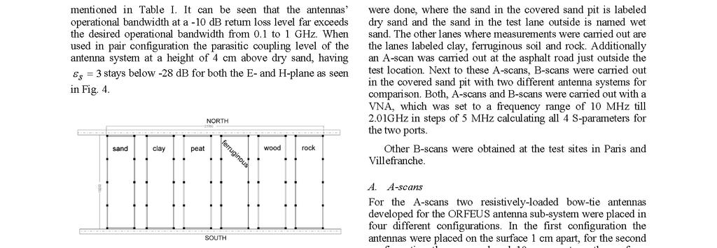
66 66

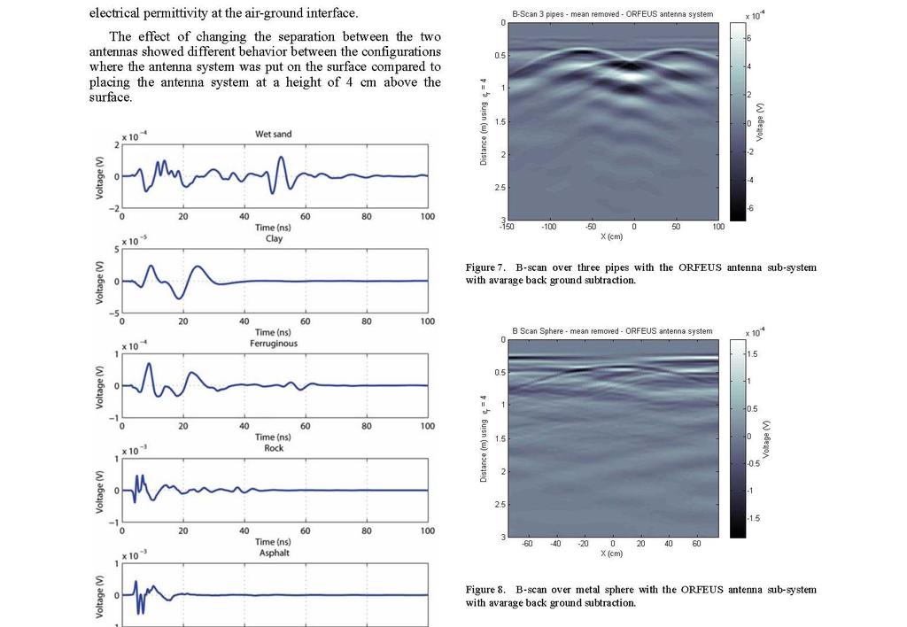
67 67

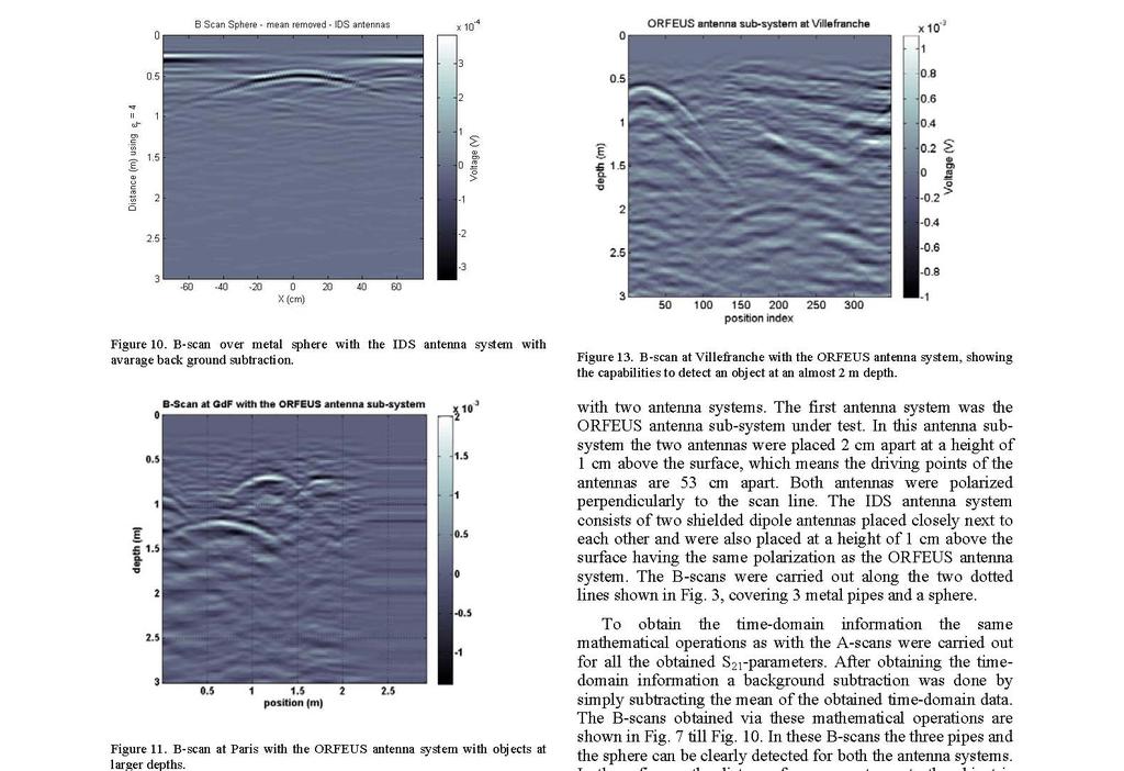
68 68

69 69

70 B. 70

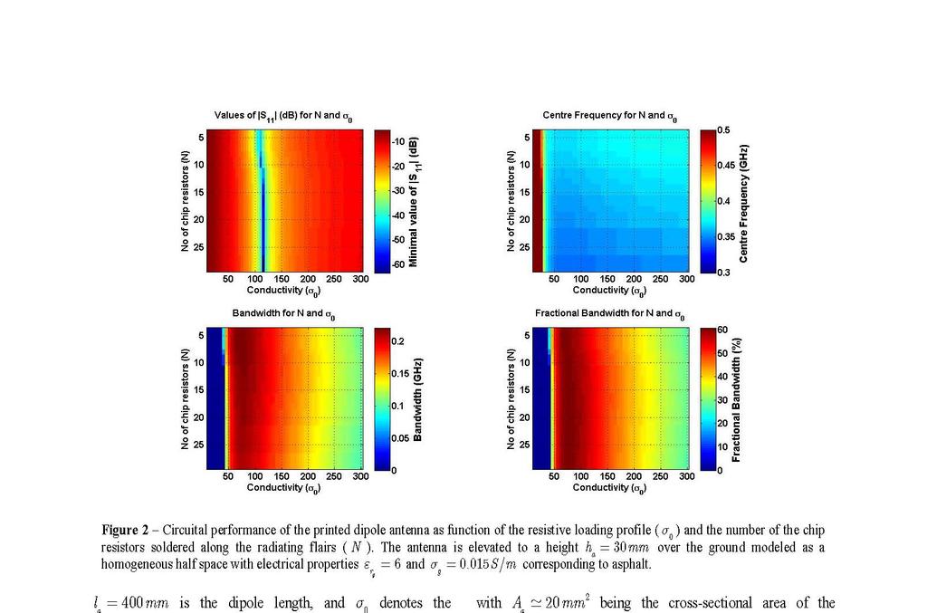
71 71

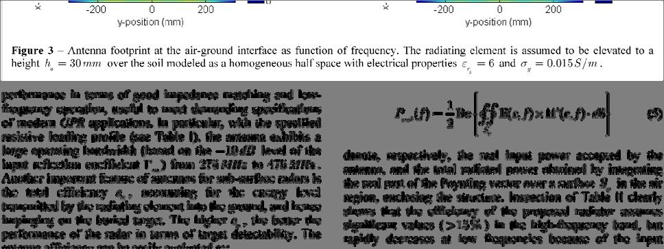
72 72

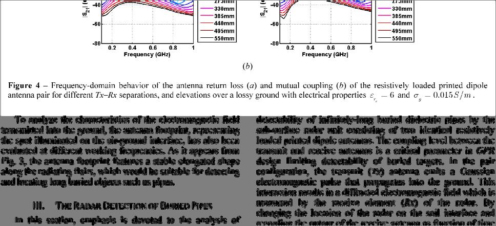
73 73

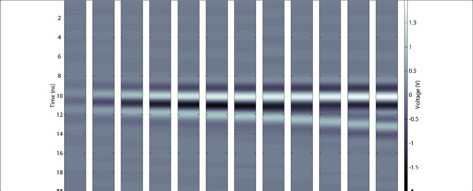
74 74

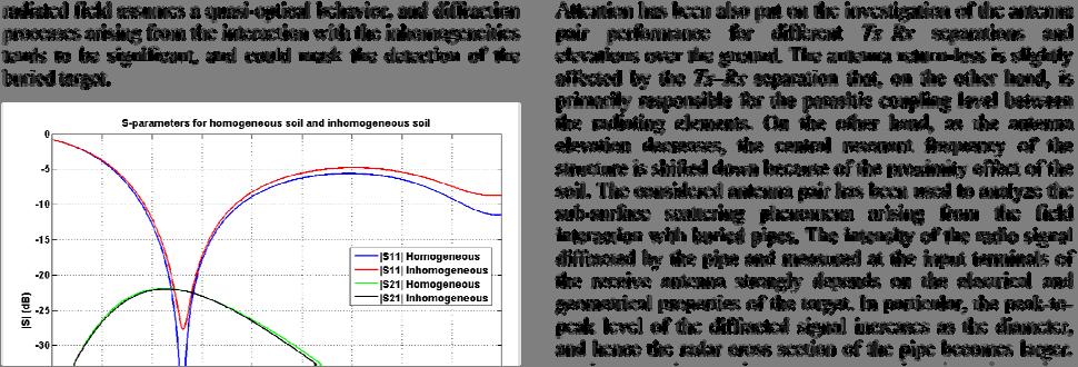
75 75

76 C. Shielding By shielding an antenna it is possible to reduce the Electromagnetic Interference (EMI) caused by the antenna on other objects in the surroundings. Also the effect of other radiating objects on the antennas is reduced. Shielding of an antenna can be done by placing a metal structure around the antenna in he areas where you want to block the radiation, doing this will however introduce spurious reflections in the antenna cavity. To reduce these spurious reflections in the antenna cavity an absorbing material is needed. Different materials have been investigated to find the best configuration for the cavity of a resistivelyloaded bow-tie antenna operating in the frequency range from 100 MHz to 1 GHz [1]. The aim of this experimental research was to reduce the level of back-radiation in this frequency range. The investigated materials are ferrite tiles and radar absorbing material (RAM) which are displayed in Figure 1. Figure 1 Eccosorb FT-04 ferrite tiles (left) and Eccosorb AN-79 absorbing foam (right). The ferrite tiles measure 10 cm by 10 cm, having a thickness of 10 mm, each tile weighs 0.3 Kg, and features a normal-incidence reflectivity below -10dB in the MHz band. The RAM is a lightweight, flexible absorber, designed to reflect less than -20 db of the normal incident energy above 600 MHz. The material comes in 61 cm x 61 cm panels with a thickness of cm The advantage of the tiles is the reduced size but comes at the cost of extra weight, while the foam is big in volume but very light. It was found that a configuration containing ferrite tiles gave the best performance. With the ferrite tiles two configurations have been tested where the ferrite tiles were directly placed behind the antenna and one configuration where there was a 2 cm thick piece of foam between the tiles and the antenna [2]. Also a configuration with an empty cavity was tested for comparison, but both configurations with the ferrite tiles showed a larger reduction of energy as seen in Figure 2 In the case of separating the antenna and the ferrite tiles with foam the return loss did fluctuate more due to internal resonances, but the average level stayed about the same. The frequency response of both configurations was also tested by placing a loop antenna at a distance of 3 m. In the case of the 2 cm separation between the tiles and the bow-tie antenna the coupling levels were the highest for vertical and horizontal polarization. Hence this configuration had the best performance and preference for the implementation of the cavity. The same experiment was repeated for two bow-tie antennas at different distances indicating the same result for the coupling. These measurements indicate that using ferrite tiles are the best option for absorbing energy in the frequency range from 100 MHz to 1 GHz. They allow for compact shielding in comparison with using radar absorbing foam. The tiles however must not be placed directly on the antenna as they will influence antenna behaviour to much. 76