1.3 Density Curves and Normal Distributions
|
|
|
- Clarissa Norton
- 5 years ago
- Views:
Transcription
1 1.3 Density Curves and Normal Distributions Ulrich Hoensch Tuesday, January 22, 2013
 the acidity or rainwater; (b) the survival time")
2 Fitting Density Curves to Histograms Advanced statistical software (NOT Microsoft Excel) can produce smoothed versions of histograms. Example The following are histograms and corresponding density curves for data representing: (a) the acidity or rainwater; (b) the survival time of Guinea pigs.
3 Fitting Density Curves to Histograms When fitting a density curve to a histogram, we want that for any interval on the horizontal axis that spans the width of a collection of rectangles, the following holds: area of rectangles area under density curve. This requirement follows from the more general fact that for both histograms and density curves, area = proportion.
4 Definition of Density Curve A density curve is a curve that is always on or above the horizontal axis and has area exactly 1 underneath it. In addition, we have that for any two values a and b on the horizontal axis, area below the density curve between a and b proportion of observations that fall between a and b.
5 Median of a Density Curve The median of a density curve is the point M on the horizontal axis so that the area below the density curve and to the left of M is 50% (and consequently the area to the right is also 50%) Median
6 Percentiles of a Density Curve The pth percentile of a density curve is the point P on the horizontal axis so that p percent of the area below the density curve lie to the left of P. The inter-quartile range is consequently the extent of the middle 50% of the area. 50 Q 1 Q 3
7 Mean of a Density Curve The mean of a density curve is the balance point of the curve: if the area below the curve were made of a solid material, the mean would correspond to the position of the fulcrum when balancing it:
8 Mean and Median of a Density Curve Unless a density curve is symmetric, the mean is not equal to the median. For right-skewed distributions the mean is larger than the median; For left-skewed distributions the mean is smaller than the median.
9 Normal Distributions Normal curves are the density functions of normal distributions. They have the following general shape. They are symmetric, unimodal (have only one peak), and bell-shaped. The mean is denoted by the symbol µ (small Greek letter mu ), and the standard deviation is denoted by the symbol σ (small Greek letter sigma ). On either side of the mean there are two points, called inflection points where the curve makes the transition from bending upwards to bending downwards, and vice versa. The standard deviation σ is the horizontal distance from the mean µ to these inflection points.
10 Normal Distributions Two normal curves are shown here.

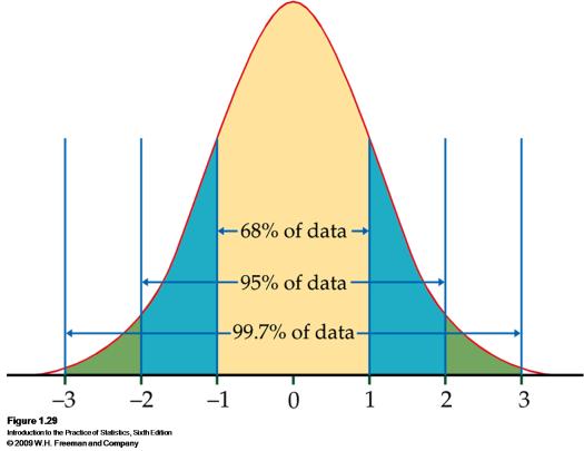
11 The Rule
12 Example: Height of Young Women The height of young women aged 18 to 24 is approximately normally distributed with mean µ = 64.5 inches and standard deviation σ = 2.5 inches. We write X N(µ, σ) if a variable X has a normal distribution with mean µ and standard deviation σ. Consequently, we have that for the height X of young women, X N(64.5, 2.5).

13 Example: Height of Young Women Find the following, using a TI-83/TI-83 Plus/TI-84 Plus calculator: The percentage of women that are between 60 and 65 inches tall. 1. Type [2ND] VARS (DISTR), select 2: normalcdf(.
14 Example: Height of Young Women 2. Type normalcdf(60,65,64.5,2.5) and press ENTER. 3. The proportion is , so the percentage of women who are between 60 and 65 inches tall is about 54.3%. This means, the shaded area is 54.3%. 54.3% Note: The general syntax for finding the proportion between a and b is normalcdf(a,b,µ,σ).
15 Example: Height of Young Women Find the percentage of who are taller than 62 inches. 1. Type [2ND] VARS (DISTR), select 2: normalcdf(. 2. Type normalcdf(62, ,64.5,2.5). (The number can be replaced by any very large positive number.) 3. Press ENTER. The proportion is , so the percentage of women who are taller than 62 inches is about 84.1%. 84.1%
16 Example: Height of Young Women What is the cutoff score for the top 10% (i.e. the 90th percentile)? 1. Type [2ND] VARS (DISTR), select 3: invnorm(. 2. Type invnorm(0.9,64.5,2.5) and press ENTER.
17 Example: Height of Young Women 3. The percentile is , so 90% of women are shorter than 67.7 inches (and 10% are taller than 67.7 inches). 90% The general syntax for finding the cutoff so that the proportion p of observations fall below this cutoff is invnorm(p,µ,σ).
18 Example: Height of Young Women Find range of the middle 80% of the distribution. This means we need to find the 10th and the 90th percentile. 80% 1. The 90th percentile was computed above, it is Type invnorm(0.1,64.5,2.5) to find the 10th percentile. It is So the middle 80% of the heights ranges from 61.3 inches to 67.7 inches.
1.3 Density Curves and Normal Distributions
 1.3 Density Curves and Normal Distributions Ulrich Hoensch Tuesday, September 11, 2012 Fitting Density Curves to Histograms Advanced statistical software (NOT Microsoft Excel) can produce smoothed versions
1.3 Density Curves and Normal Distributions. Ulrich Hoensch MAT210 Rocky Mountain College Billings, MT 59102
 1.3 Density Curves and Normal Distributions Ulrich Hoensch MAT210 Rocky Mountain College Billings, MT 59102 Fitting Density Curves to Histograms Advanced statistical software (NOT Microsoft Excel) can
Chapter 3. The Normal Distributions. BPS - 5th Ed. Chapter 3 1
 Chapter 3 The Normal Distributions BPS - 5th Ed. Chapter 3 1 Density Curves Example: here is a histogram of vocabulary scores of 947 seventh graders. The smooth curve drawn over the histogram is a mathematical
Density Curves. Chapter 3. Density Curves. Density Curves. Density Curves. Density Curves. Basic Practice of Statistics - 3rd Edition.
 Chapter 3 The Normal Distributions Example: here is a histogram of vocabulary scores of 947 seventh graders. The smooth curve drawn over the histogram is a mathematical idialization for the distribution.
CHAPTER 13A. Normal Distributions
 CHAPTER 13A Normal Distributions SO FAR We always want to plot our data. We make a graph, usually a histogram or a stemplot. We want to look for an overall pattern (shape, center, spread) and for any striking
2.2 More on Normal Distributions and Standard Normal Calculations
 The distribution of heights of adult American men is approximately normal with mean 69 inches and standard deviation 2.5 inches. Use the 68-95-99.7 rule to answer the following questions: What percent
Female Height. Height (inches)
") Math 111 Normal distribution NAME: Consider the histogram detailing female height. The mean is 6 and the standard deviation is 2.. We will use it to introduce and practice the ideas of normal distributions.
Math 111 Normal distribution NAME: Consider the histogram detailing female height. The mean is 6 and the standard deviation is 2.. We will use it to introduce and practice the ideas of normal distributions.
Math 247: Continuous Random Variables: The Uniform Distribution (Section 6.1) and The Normal Distribution (Section 6.2)
 and The Normal Distribution (Section 6.2)") Math 247: Continuous Random Variables: The Uniform Distribution (Section 6.1) and The Normal Distribution (Section 6.2) The Uniform Distribution Example: If you are asked to pick a number from 1 to 10
Math 247: Continuous Random Variables: The Uniform Distribution (Section 6.1) and The Normal Distribution (Section 6.2) The Uniform Distribution Example: If you are asked to pick a number from 1 to 10
Rule. Describing variability using the Rule. Standardizing with Z scores
 Lecture 8: Bell-Shaped Curves and Other Shapes Unimodal and symmetric, bell shaped curve Most variables are nearly normal, but real data is never exactly normal Denoted as N(µ, σ) Normal with mean µ and
Section 1.5 Graphs and Describing Distributions
 Section 1.5 Graphs and Describing Distributions Data can be displayed using graphs. Some of the most common graphs used in statistics are: Bar graph Pie Chart Dot plot Histogram Stem and leaf plot Box
Probability WS 1 Counting , , , a)625 b)1050c) a)20358,520 b) 1716 c) 55,770
625 b)1050c) a)20358,520 b) 1716 c) 55,770") Probability WS 1 Counting 1.28 2.13,800 3.5832 4.30 5.. 15 7.72 8.33, 5 11. 15,504 12. a)25 b)1050c)2275 13. a)20358,520 b) 171 c) 55,770 d) 12,271,512e) 1128 f) 17 14. 438 15. 2,000 1. 11,700 17. 220,
Probability WS 1 Counting 1.28 2.13,800 3.5832 4.30 5.. 15 7.72 8.33, 5 11. 15,504 12. a)25 b)1050c)2275 13. a)20358,520 b) 171 c) 55,770 d) 12,271,512e) 1128 f) 17 14. 438 15. 2,000 1. 11,700 17. 220,
(Notice that the mean doesn t have to be a whole number and isn t normally part of the original set of data.)
") One-Variable Statistics Descriptive statistics that analyze one characteristic of one sample Where s the middle? How spread out is it? Where do different pieces of data compare? To find 1-variable statistics
One-Variable Statistics Descriptive statistics that analyze one characteristic of one sample Where s the middle? How spread out is it? Where do different pieces of data compare? To find 1-variable statistics
Chapter 4. Displaying and Summarizing Quantitative Data. Copyright 2012, 2008, 2005 Pearson Education, Inc.
 Chapter 4 Displaying and Summarizing Quantitative Data Copyright 2012, 2008, 2005 Pearson Education, Inc. Dealing With a Lot of Numbers Summarizing the data will help us when we look at large sets of quantitative
MULTIPLE CHOICE. Choose the one alternative that best completes the statement or answers the question. B) Blood type Frequency
 Blood type Frequency") MATH 1342 Final Exam Review Name Construct a frequency distribution for the given qualitative data. 1) The blood types for 40 people who agreed to participate in a medical study were as follows. 1) O A
MATH 1342 Final Exam Review Name Construct a frequency distribution for the given qualitative data. 1) The blood types for 40 people who agreed to participate in a medical study were as follows. 1) O A
1.1 Displaying Distributions with Graphs, Continued
 1.1 Displaying Distributions with Graphs, Continued Ulrich Hoensch Thursday, January 10, 2013 Histograms Constructing a frequency table involves breaking the range of values of a quantitative variable
Confidence Intervals. Class 23. November 29, 2011
 Confidence Intervals Class 23 November 29, 2011 Last Time When sampling from a population in which 30% of individuals share a certain characteristic, we identified the reasonably likely values for the
Descriptive Statistics II. Graphical summary of the distribution of a numerical variable. Boxplot
 MAT 2379 (Spring 2012) Descriptive Statistics II Graphical summary of the distribution of a numerical variable We will present two types of graphs that can be used to describe the distribution of a numerical
November 11, Chapter 8: Probability: The Mathematics of Chance
 Chapter 8: Probability: The Mathematics of Chance November 11, 2013 Last Time Probability Models and Rules Discrete Probability Models Equally Likely Outcomes Probability Rules Probability Rules Rule 1.
Numerical: Data with quantity Discrete: whole number answers Example: How many siblings do you have?
 Types of data Numerical: Data with quantity Discrete: whole number answers Example: How many siblings do you have? Continuous: Answers can fall anywhere in between two whole numbers. Usually any type of
Sections Descriptive Statistics for Numerical Variables
 Math 243 Sections 2.1.2-2.2.5 Descriptive Statistics for Numerical Variables A framework to describe quantitative data: Describe the Shape, Center and Spread, and Unusual Features Shape How is the data
This page intentionally left blank
 Appendix E Labs This page intentionally left blank Dice Lab (Worksheet) Objectives: 1. Learn how to calculate basic probabilities of dice. 2. Understand how theoretical probabilities explain experimental
Outline. Drawing the Graph. 1 Homework Review. 2 Introduction. 3 Histograms. 4 Histograms on the TI Assignment
 Lecture 14 Section 4.4.4 on Hampden-Sydney College Fri, Sep 18, 2009 Outline 1 on 2 3 4 on 5 6 Even-numbered on Exercise 4.25, p. 249. The following is a list of homework scores for two students: Student
CREATED BY SHANNON MARTIN GRACEY 107 STATISTICS GUIDED NOTEBOOK/FOR USE WITH MARIO TRIOLA S TEXTBOOK ESSENTIALS OF STATISTICS, 4TH ED.
 c. Between 1.00 and 3.00 e. Greater than 3.68 d. Between -2.87 and 1.34 USING THE TI-84 CREATED BY SHANNON MARTIN GRACEY 107 FINDING z SCORES WITH KNOWN AREAS 1. Draw a bell-shaped curve and the under
Possible responses to the 2015 AP Statistics Free Resposne questions, Draft #2. You can access the questions here at AP Central.
 Possible responses to the 2015 AP Statistics Free Resposne questions, Draft #2. You can access the questions here at AP Central. Note: I construct these as a service for both students and teachers to start
Chapter 1: Stats Starts Here Chapter 2: Data
 Chapter 1: Stats Starts Here Chapter 2: Data Statistics data, datum variation individual respondent subject participant experimental unit observation variable categorical quantitative Calculator Skills:
Univariate Descriptive Statistics
 Univariate Descriptive Statistics Displays: pie charts, bar graphs, box plots, histograms, density estimates, dot plots, stemleaf plots, tables, lists. Example: sea urchin sizes Boxplot Histogram Urchin
Chpt 2. Frequency Distributions and Graphs. 2-3 Histograms, Frequency Polygons, Ogives / 35
 Chpt 2 Frequency Distributions and Graphs 2-3 Histograms, Frequency Polygons, Ogives 1 Chpt 2 Homework 2-3 Read pages 48-57 p57 Applying the Concepts p58 2-4, 10, 14 2 Chpt 2 Objective Represent Data Graphically
AP Statistics Composition Book Review Chapters 1 2
 AP Statistics Composition Book Review Chapters 1 2 Terms/vocabulary: Explain each term with in the STATISTICAL context. Bar Graph Bimodal Categorical Variable Density Curve Deviation Distribution Dotplot
HOMEWORK 3 Due: next class 2/3
 HOMEWORK 3 Due: next class 2/3 1. Suppose the scores on an achievement test follow an approximately symmetric mound-shaped distribution with mean 500, min = 350, and max = 650. Which of the following is
Chapter 10. Definition: Categorical Variables. Graphs, Good and Bad. Distribution
 Chapter 10 Graphs, Good and Bad Chapter 10 3 Distribution Definition: Tells what values a variable takes and how often it takes these values Can be a table, graph, or function Categorical Variables Places
Chapter 11. Sampling Distributions. BPS - 5th Ed. Chapter 11 1
 Chapter 11 Sampling Distributions BPS - 5th Ed. Chapter 11 1 Sampling Terminology Parameter fixed, unknown number that describes the population Example: population mean Statistic known value calculated
Displaying Distributions with Graphs
 Displaying Distributions with Graphs Recall that the distribution of a variable indicates two things: (1) What value(s) a variable can take, and (2) how often it takes those values. Example 1: Weights
Data About Us Practice Answers
 Investigation Additional Practice. a. The mode is. While the data set is a collection of numbers, there is no welldefined notion of the center for this distribution. So the use of mode as a typical number
Chapter 11. Sampling Distributions. BPS - 5th Ed. Chapter 11 1
 Chapter 11 Sampling Distributions BPS - 5th Ed. Chapter 11 1 Sampling Terminology Parameter fixed, unknown number that describes the population Statistic known value calculated from a sample a statistic
Objectives. Organizing Data. Example 1. Making a Frequency Distribution. Solution
 Lesson 7.2 Objectives Organize data into a frequency distribution. Find the mean using a frequency distribution. Create a histogram from a frequency distribution. Frequency Distributions In Lesson 7.1,
Section 1: Data (Major Concept Review)
") Section 1: Data (Major Concept Review) Individuals = the objects described by a set of data variable = characteristic of an individual weight height age IQ hair color eye color major social security #
Section 1: Data (Major Concept Review) Individuals = the objects described by a set of data variable = characteristic of an individual weight height age IQ hair color eye color major social security #
IE 361 Module 36. Process Capability Analysis Part 1 (Normal Plotting) Reading: Section 4.1 Statistical Methods for Quality Assurance
 Reading: Section 4.1 Statistical Methods for Quality Assurance") IE 361 Module 36 Process Capability Analysis Part 1 (Normal Plotting) Reading: Section 4.1 Statistical Methods for Quality Assurance ISU and Analytics Iowa LLC (ISU and Analytics Iowa LLC) IE 361 Module
IE 361 Module 36 Process Capability Analysis Part 1 (Normal Plotting) Reading: Section 4.1 Statistical Methods for Quality Assurance ISU and Analytics Iowa LLC (ISU and Analytics Iowa LLC) IE 361 Module
Symmetric (Mean and Standard Deviation)
") Summary: Unit 2 & 3 Distributions for Quantitative Data Topics covered in Module 2: How to calculate the Mean, Median, IQR Shapes of Histograms, Dotplots, Boxplots Know the difference between categorical
Summary: Unit 2 & 3 Distributions for Quantitative Data Topics covered in Module 2: How to calculate the Mean, Median, IQR Shapes of Histograms, Dotplots, Boxplots Know the difference between categorical
Math 113-All Sections Final Exam May 6, 2013
 Name Math 3-All Sections Final Exam May 6, 23 Answer questions on the scantron provided. The scantron should be the same color as this page. Be sure to encode your name, student number and SECTION NUMBER
To describe the centre and spread of a univariate data set by way of a 5-figure summary and visually by a box & whisker plot.
 Five Figure Summary Teacher Notes & Answers 7 8 9 10 11 12 TI-Nspire Investigation Student 60 min Aim To describe the centre and spread of a univariate data set by way of a 5-figure summary and visually
Chapter 4. September 08, appstats 4B.notebook. Displaying Quantitative Data. Aug 4 9:13 AM. Aug 4 9:13 AM. Aug 27 10:16 PM.
 Objectives: Students will: Chapter 4 1. Be able to identify an appropriate display for any quantitative variable: stem leaf plot, time plot, histogram and dotplot given a set of quantitative data. 2. Be
Q Scheme Marks AOs. 1a All points correctly plotted. B2 1.1b 2nd Draw and interpret scatter diagrams for bivariate data.
 1a All points correctly plotted. B2 2nd Draw and interpret scatter diagrams for bivariate data. 1b The points lie reasonably close to a straight line (o.e.). 2.4 2nd Draw and interpret scatter diagrams
MAT Mathematics in Today's World
 MAT 1000 Mathematics in Today's World Last Time 1. Three keys to summarize a collection of data: shape, center, spread. 2. The distribution of a data set: which values occur, and how often they occur 3.
Chapter 3. Graphical Methods for Describing Data. Copyright 2005 Brooks/Cole, a division of Thomson Learning, Inc.
 Chapter 3 Graphical Methods for Describing Data 1 Frequency Distribution Example The data in the column labeled vision for the student data set introduced in the slides for chapter 1 is the answer to the
Name: Date: Period: Histogram Worksheet
 Name: Date: Period: Histogram Worksheet 1 5. For the following five histograms, list at least 3 characteristics that describe each histogram (consider symmetric, skewed to left, skewed to right, unimodal,
CS 147: Computer Systems Performance Analysis
 CS 147: Computer Systems Performance Analysis Mistakes in Graphical Presentation CS 147: Computer Systems Performance Analysis Mistakes in Graphical Presentation 1 / 45 Overview Excess Information Multiple
Chapter 1. Statistics. Individuals and Variables. Basic Practice of Statistics - 3rd Edition. Chapter 1 1. Picturing Distributions with Graphs
 Chapter 1 Picturing Distributions with Graphs BPS - 3rd Ed. Chapter 1 1 Statistics Statistics is a science that involves the extraction of information from numerical data obtained during an experiment
Measurement over a Short Distance. Tom Mathew
 Measurement over a Short Distance Tom Mathew Outline Introduction Data Collection Methods Data Analysis Conclusion Introduction Determine Fundamental Traffic Parameter Data Collection and Interpretation
(3 pts) 1. Which statements are usually true of a left-skewed distribution? (circle all that are correct)
 1. Which statements are usually true of a left-skewed distribution? (circle all that are correct)") STAT 451 - Practice Exam I Name (print): Section: This is a practice exam - it s a representative sample of problems that may appear on the exam and also substantially longer than the in-class exam. It
STAT 451 - Practice Exam I Name (print): Section: This is a practice exam - it s a representative sample of problems that may appear on the exam and also substantially longer than the in-class exam. It
10 Wyner Statistics Fall 2013
 1 Wyner Statistics Fall 213 CHAPTER TWO: GRAPHS Summary Terms Objectives For research to be valuable, it must be shared. The fundamental aspect of a good graph is that it makes the results clear at a glance.
1) What is the total area under the curve? 1) 2) What is the mean of the distribution? 2)
 What is the total area under the curve? 1) 2) What is the mean of the distribution? 2)") Math 1090 Test 2 Review Worksheet Ch5 and Ch 6 Name Use the following distribution to answer the question. 1) What is the total area under the curve? 1) 2) What is the mean of the distribution? 2) 3) Estimate
Math 1090 Test 2 Review Worksheet Ch5 and Ch 6 Name Use the following distribution to answer the question. 1) What is the total area under the curve? 1) 2) What is the mean of the distribution? 2) 3) Estimate
STK110. Chapter 2: Tabular and Graphical Methods Lecture 1 of 2. ritakeller.com. mathspig.wordpress.com
 STK110 Chapter 2: Tabular and Graphical Methods Lecture 1 of 2 ritakeller.com mathspig.wordpress.com Frequency distribution Example Data from a sample of 50 soft drink purchases Frequency Distribution
PASS Sample Size Software
 Chapter 945 Introduction This section describes the options that are available for the appearance of a histogram. A set of all these options can be stored as a template file which can be retrieved later.
Describing Data Visually. Describing Data Visually. Describing Data Visually 9/28/12. Applied Statistics in Business & Economics, 4 th edition
 A PowerPoint Presentation Package to Accompany Applied Statistics in Business & Economics, 4 th edition David P. Doane and Lori E. Seward Prepared by Lloyd R. Jaisingh Describing Data Visually Chapter
Frequency Distribution and Graphs
 Chapter 2 Frequency Distribution and Graphs 2.1 Organizing Qualitative Data Denition 2.1.1 A categorical frequency distribution lists the number of occurrences for each category of data. Example 2.1.1
11 Wyner Statistics Fall 2018
 11 Wyner Statistics Fall 218 CHAPTER TWO: GRAPHS Review September 19 Test September 28 For research to be valuable, it must be shared, and a graph can be an effective way to do so. The fundamental aspect
Mean for population data: x = the sum of all values. N = the population size n = the sample size, µ = the population mean. x = the sample mean
 MEASURE OF CENTRAL TENDENCY MEASURS OF CENTRAL TENDENCY Ungrouped Data Measurement Mean Mean for population data: Mean for sample data: x N x x n where: x = the sum of all values N = the population size
Chapter 4 Displaying and Describing Quantitative Data
 Chapter 4 Displaying and Describing Quantitative Data Overview Key Concepts Be able to identify an appropriate display for any quantitative variable. Be able to guess the shape of the distribution of a
Math Exam 2 Review. NOTE: For reviews of the other sections on Exam 2, refer to the first page of WIR #4 and #5.
 Math 166 Fall 2008 c Heather Ramsey Page 1 Math 166 - Exam 2 Review NOTE: For reviews of the other sections on Exam 2, refer to the first page of WIR #4 and #5. Section 3.2 - Measures of Central Tendency
IE 361 Module 17. Process Capability Analysis: Part 1. Reading: Sections 5.1, 5.2 Statistical Quality Assurance Methods for Engineers
 IE 361 Module 17 Process Capability Analysis: Part 1 Reading: Sections 5.1, 5.2 Statistical Quality Assurance Methods for Engineers Prof. Steve Vardeman and Prof. Max Morris Iowa State University Vardeman
Mathematics (Project Maths)
") 2010. M128 S Coimisiún na Scrúduithe Stáit State Examinations Commission Leaving Certificate Examination Sample Paper Mathematics (Project Maths) Paper 2 Ordinary Level Time: 2 hours, 30 minutes 300 marks
2010. M128 S Coimisiún na Scrúduithe Stáit State Examinations Commission Leaving Certificate Examination Sample Paper Mathematics (Project Maths) Paper 2 Ordinary Level Time: 2 hours, 30 minutes 300 marks
CHAPTER 6 PROBABILITY. Chapter 5 introduced the concepts of z scores and the normal curve. This chapter takes
 CHAPTER 6 PROBABILITY Chapter 5 introduced the concepts of z scores and the normal curve. This chapter takes these two concepts a step further and explains their relationship with another statistical concept
c. If you roll the die six times what are your chances of getting at least one d. roll.
 1. Find the area under the normal curve: a. To the right of 1.25 (100-78.87)/2=10.565 b. To the left of -0.40 (100-31.08)/2=34.46 c. To the left of 0.80 (100-57.63)/2=21.185 d. Between 0.40 and 1.30 for
Variables. Lecture 13 Sections Wed, Sep 16, Hampden-Sydney College. Displaying Distributions - Quantitative.
 - - Lecture 13 Sections 4.4.1-4.4.3 Hampden-Sydney College Wed, Sep 16, 2009 Outline - 1 2 3 4 5 6 7 Even-numbered - Exercise 4.7, p. 226. According to the National Center for Health Statistics, in the
USE OF BASIC ELECTRONIC MEASURING INSTRUMENTS Part II, & ANALYSIS OF MEASUREMENT ERROR 1
 EE 241 Experiment #3: USE OF BASIC ELECTRONIC MEASURING INSTRUMENTS Part II, & ANALYSIS OF MEASUREMENT ERROR 1 PURPOSE: To become familiar with additional the instruments in the laboratory. To become aware
University of Connecticut Department of Mathematics
 University of Connecticut Department of Mathematics Math 1070 Sample Exam 2 Fall 2014 Name: Instructor Name: Section: Exam 2 will cover Sections 4.6-4.7, 5.3-5.4, 6.1-6.4, and F.1-F.3. This sample exam
i. Are the shapes of the two distributions fundamentally alike or fundamentally different?
 Unit 5 Lesson 1 Investigation 1 Name: Investigation 1 Shapes of Distributions Every day, people are bombarded by data on television, on the Internet, in newspapers, and in magazines. For example, states
Section 5.2 Graphs of the Sine and Cosine Functions
 Section 5.2 Graphs of the Sine and Cosine Functions We know from previously studying the periodicity of the trigonometric functions that the sine and cosine functions repeat themselves after 2 radians.
Chapter 2. Organizing Data. Slide 2-2. Copyright 2012, 2008, 2005 Pearson Education, Inc.
 Chapter 2 Organizing Data Slide 2-2 Section 2.1 Variables and Data Slide 2-3 Definition 2.1 Variables Variable: A characteristic that varies from one person or thing to another. Qualitative variable: A
Spatial Filtering of Surface Profile Data
 Spatial Filtering of Surface Profile Data/1 Spatial Filtering of Surface Profile Data Chapman Technical Note-TG-1 spat_fil.doc Rev-01-09 Spatial Filtering of Surface Profile Data/2 Explanation of Filtering
Find the following for the Weight of Football Players. Sample standard deviation n=
 Find the following for the Weight of Football Players x Sample standard deviation n= Fun Coming Up! 3-3 Measures of Position Z-score Percentile Quartile Outlier Bluman, Chapter 3 3 Measures of Position:
DESCRIBING DATA. Frequency Tables, Frequency Distributions, and Graphic Presentation
 DESCRIBING DATA Frequency Tables, Frequency Distributions, and Graphic Presentation Raw Data A raw data is the data obtained before it is being processed or arranged. 2 Example: Raw Score A raw score is
MDM4U Some Review Questions
 1. Expand and simplify the following expressions. a) ( y 1) 7 b) ( 3x 2) 6 2x + 3 5 2. In the expansion of ( ) 9 MDM4U Some Review Questions, find a) the 6 th term b) 12 the term containing x n + 7 n +
MATH , Summer I Homework - 05
 MATH 2300-02, Summer I - 200 Homework - 05 Name... TRUE/FALSE. Write 'T' if the statement is true and 'F' if the statement is false. Due on Tuesday, October 26th ) True or False: If p remains constant
University of California, Berkeley, Statistics 20, Lecture 1. Michael Lugo, Fall Exam 2. November 3, 2010, 10:10 am - 11:00 am
 University of California, Berkeley, Statistics 20, Lecture 1 Michael Lugo, Fall 2010 Exam 2 November 3, 2010, 10:10 am - 11:00 am Name: Signature: Student ID: Section (circle one): 101 (Joyce Chen, TR
Math 58. Rumbos Fall Solutions to Exam Give thorough answers to the following questions:
 Math 58. Rumbos Fall 2008 1 Solutions to Exam 2 1. Give thorough answers to the following questions: (a) Define a Bernoulli trial. Answer: A Bernoulli trial is a random experiment with two possible, mutually
Section 5.2 Graphs of the Sine and Cosine Functions
 A Periodic Function and Its Period Section 5.2 Graphs of the Sine and Cosine Functions A nonconstant function f is said to be periodic if there is a number p > 0 such that f(x + p) = f(x) for all x in
Lesson 17. Student Outcomes. Lesson Notes. Classwork. Example 1 (5 10 minutes): Predicting the Pattern in the Residual Plot
: Predicting the Pattern in the Residual Plot") Student Outcomes Students use a graphing calculator to construct the residual plot for a given data set. Students use a residual plot as an indication of whether the model used to describe the relationship
Student Outcomes Students use a graphing calculator to construct the residual plot for a given data set. Students use a residual plot as an indication of whether the model used to describe the relationship
Chapter Displaying Graphical Data. Frequency Distribution Example. Graphical Methods for Describing Data. Vision Correction Frequency Relative
 Chapter 3 Graphical Methods for Describing 3.1 Displaying Graphical Distribution Example The data in the column labeled vision for the student data set introduced in the slides for chapter 1 is the answer
Plotting Points & The Cartesian Plane. Scatter Plots WS 4.2. Line of Best Fit WS 4.3. Curve of Best Fit WS 4.4. Graphing Linear Relations WS 4.
 UNIT 4 - GRAPHING RELATIONS Date Lesson Topic HW Nov. 3 4.1 Plotting Points & The Cartesian Plane WS 4.1 Nov. 6 4.1 Plotting Points & The Cartesian Plane WS 4.1-II Nov. 7 4.2 Scatter Plots WS 4.2 Nov.
EE EXPERIMENT 3 RESISTIVE NETWORKS AND COMPUTATIONAL ANALYSIS INTRODUCTION
 EE 2101 - EXPERIMENT 3 RESISTIVE NETWORKS AND COMPUTATIONAL ANALYSIS INTRODUCTION The resistors used in this laboratory are carbon composition resistors, consisting of graphite or some other type of carbon
!"#$%&'("&)*("*+,)-(#'.*/$'-0%$1$"&-!!!"#$%&'(!"!!"#$%"&&'()*+*!
*(*+,)-(#'.*/$'-0%$1$&-!!!#$%&'(!!!#$%&&'()*+*!") !"#$%&'("&)*("*+,)-(#'.*/$'-0%$1$"&-!!!"#$%&'(!"!!"#$%"&&'()*+*! In this Module, we will consider dice. Although people have been gambling with dice and related apparatus since at least 3500 BCE, amazingly
!"#$%&'("&)*("*+,)-(#'.*/$'-0%$1$"&-!!!"#$%&'(!"!!"#$%"&&'()*+*! In this Module, we will consider dice. Although people have been gambling with dice and related apparatus since at least 3500 BCE, amazingly
Chapter 2. Describing Distributions with Numbers. BPS - 5th Ed. Chapter 2 1
 Chapter 2 Describing Distributions with Numbers BPS - 5th Ed. Chapter 2 1 Numerical Summaries Center of the data mean median Variation range quartiles (interquartile range) variance standard deviation
Exploring Data Patterns. Run Charts, Frequency Tables, Histograms, Box Plots
 Exploring Data Patterns Run Charts, Frequency Tables, Histograms, Box Plots 1 Topics I. Exploring Data Patterns - Tools A. Run Chart B. Dot Plot C. Frequency Table and Histogram D. Box Plot II. III. IV.
Exam Time. Final Exam Review. TR class Monday December 9 12:30 2:30. These review slides and earlier ones found linked to on BlackBoard
 Final Exam Review These review slides and earlier ones found linked to on BlackBoard Bring a photo ID card: Rocket Card, Driver's License Exam Time TR class Monday December 9 12:30 2:30 Held in the regular
Core Connections, Course 2 Checkpoint Materials
 Core Connections, Course Checkpoint Materials Notes to Students (and their Teachers) Students master different skills at different speeds. No two students learn exactly the same way at the same time. At
16 Histograms. Using Histograms to Reveal Distribution
 16 Histograms Using Histograms to Reveal Distribution The Histogram math function enhances understanding of the distribution of measured parameters (see the Disk Drive Analyzer Reference Manual for more
Chapter 11. Sampling Distributions. BPS - 5th Ed. Chapter 11 1
 Chapter 11 Sampling Distributions BPS - 5th Ed. Chapter 11 1 Sampling Terminology Parameter fixed, unknown number that describes the population Statistic known value calculated from a sample a statistic
Section 6.4. Sampling Distributions and Estimators
 Section 6.4 Sampling Distributions and Estimators IDEA Ch 5 and part of Ch 6 worked with population. Now we are going to work with statistics. Sample Statistics to estimate population parameters. To make
AP STATISTICS 2015 SCORING GUIDELINES
 AP STATISTICS 2015 SCORING GUIDELINES Question 6 Intent of Question The primary goals of this question were to assess a student s ability to (1) describe how sample data would differ using two different
Learning Log Title: CHAPTER 2: ARITHMETIC STRATEGIES AND AREA. Date: Lesson: Chapter 2: Arithmetic Strategies and Area
 Chapter 2: Arithmetic Strategies and Area CHAPTER 2: ARITHMETIC STRATEGIES AND AREA Date: Lesson: Learning Log Title: Date: Lesson: Learning Log Title: Chapter 2: Arithmetic Strategies and Area Date: Lesson:
Lecture Slides. Elementary Statistics Twelfth Edition. by Mario F. Triola. and the Triola Statistics Series. Section 2.2- #
 Lecture Slides Elementary Statistics Twelfth Edition and the Triola Statistics Series by Mario F. Triola Chapter 2 Summarizing and Graphing Data 2-1 Review and Preview 2-2 Frequency Distributions 2-3 Histograms
Lecture 16 Sections Tue, Sep 23, 2008
 s Lecture 16 Sections 5.3.1-5.3.3 Hampden-Sydney College Tue, Sep 23, 2008 in Outline s in 1 2 3 s 4 5 6 in 7 s Exercise 5.7, p. 312. (a) average (or mean) age for 10 adults in a room is 35 years. A 32-year-old
Test 2 SOLUTIONS (Chapters 5 7)
") Test 2 SOLUTIONS (Chapters 5 7) 10 1. I have been sitting at my desk rolling a six-sided die (singular of dice), and counting how many times I rolled a 6. For example, after my first roll, I had rolled
Test 2 SOLUTIONS (Chapters 5 7) 10 1. I have been sitting at my desk rolling a six-sided die (singular of dice), and counting how many times I rolled a 6. For example, after my first roll, I had rolled
SAMPLE. This chapter deals with the construction and interpretation of box plots. At the end of this chapter you should be able to:
 find the upper and lower extremes, the median, and the upper and lower quartiles for sets of numerical data calculate the range and interquartile range compare the relative merits of range and interquartile
MULTIPLE CHOICE. Choose the one alternative that best completes the statement or answers the question.
 Practice for Final Exam Name Identify the following variable as either qualitative or quantitative and explain why. 1) The number of people on a jury A) Qualitative because it is not a measurement or a
Exam 2 Review. Review. Cathy Poliak, Ph.D. (Department of Mathematics ReviewUniversity of Houston ) Exam 2 Review
 Exam 2 Review") Exam 2 Review Review Cathy Poliak, Ph.D. cathy@math.uh.edu Department of Mathematics University of Houston Exam 2 Review Exam 2 Review 1 / 20 Outline 1 Material Covered 2 What is on the exam 3 Examples
Exam 2 Review Review Cathy Poliak, Ph.D. cathy@math.uh.edu Department of Mathematics University of Houston Exam 2 Review Exam 2 Review 1 / 20 Outline 1 Material Covered 2 What is on the exam 3 Examples
PLC Papers Created For:
 PLC Papers Created For: Year 11 Topic Practice Paper: Histograms Histograms with unequal class widths 1 Grade 6 Objective: Construct and interpret a histogram with unequal class widths (for grouped discrete
Biggar High School Mathematics Department. S1 Block 1. Revision Booklet GOLD
 Biggar High School Mathematics Department S1 Block 1 Revision Booklet GOLD Contents MNU 3-01a MNU 3-03a MNU 3-03b Page Whole Number Calculations & Decimals 3 MTH 3-05b MTH 3-06a MTH 4-06a Multiples, Factors,