Automated level generation and difficulty rating for Trainyard

Transcription

1 Automated level generation and difficulty rating for Trainyard Master Thesis Game & Media Technology Author: Nicky Vendrig Student #: Supervisors: Prof. dr. M.J. van Kreveld Dr. M. Löffler October 2013

2 Abstract This thesis presents a framework for automatic level generation for the puzzle game Trainyard. We made a replica of this game, called Flight, and integrated the level generation framework into it. This framework is able to automatically generate levels of various difficulty. The generation of levels is divided into three components: (i) the level generator, which creates the level, (ii) the level solver, which checks the feasibility of the generated level, and (iii) the difficulty estimator, which rates the difficulty of the generated level. To test the presented framework we did two user studies: (i) a pilot study, which tested whether the difficulty ratings of the original game 1 correspond to the ratings given by the player, and (ii) a full user study, which tested whether the assigned difficulty ratings of the generated levels corresponds to the player s experience. The results of the level generation framework are very promising, levels are automatically generated, tested and rated successfully. In further research the process could be optimized to make the level generation faster and generated levels more user specific. 1 Trainyard uses stars to represent the difficulty of each level. i

3 Acknowledgements I would like to thank Prof. dr. M.J. van Kreveld and Dr. M. Löffler for the guidance during this master project. I would also like to thank all the people who participated in the user studies and those who tested the game Flight. ii

4 Contents Page 1 Introduction Problem description Project outline Thesis overview Background Trainyard Level generation Generation algorithms Our level generator Level solving Other algorithms Our level solver Difficulty estimation Process Trainyard Framework overview Level generation Mission generator Grid placement Level solver Difficulty estimator Example Implementation Flight Generation framework Level generator Level solver Difficulty estimator Results & Evaluation System analysis User studies Pilot study User study Discussion Generation framework User studies iii

5 7 Conclusion and future work Our research Future research References 42 List of Figures 45 List of Tables 47 A Original levels 48 B Generated levels 55 iv

6 Chapter 1 Introduction This chapter describes the research project and what our research questions are. Further, the scope of this research project and the structure of this thesis are described. 1.1 Problem description Puzzle games are often very limited in their provision of levels: the number of levels is limited or the levels do not meet the skill level of the player. The levels in these games are often made by hand, a time consuming business. During the development of a game time is scarce. This lack of time often means that a puzzle game does not contain many levels on its release. Extra levels are added later after the developer has finished them. In the casual (puzzle) game market it is important to keep the interest of the player. This market has a variety of games, that are often free. This allows the player to switch between games very fast and lose his interest in a game quickly. An adequate supply of levels could help to keep a player interested. The attention of the player can be kept by offering him a large set of levels, but nowadays only offering a sufficient number of levels is not enough: players demand to be challenged. Automated level generation can be used for the provision of a level set that is sufficient to keep a player attracted to the game for a longer period of time. However, a large set of automatically generated levels does not mean the player will be challenged. Every player is unique, so challenging them all with a predefined level set is not possible. Therefore it is useful to make the generated levels more user specific and meet the requirements of a single player. As said automated level generation can be useful to create large sets of user-specific levels. Important when levels are automatically generated is that every provided level is feasible. Players want to be challenged, but presenting a level that does not have a solution or is over-challenging them is annoying and the player will probably stop playing the game. Every generated level should be tested, this can be done by a computer or by a human. When a computer tests a level, it can still be over-challenging the player: a computer is able to test for every possible solution, while for a human player this is almost impossible and would take up years. To prevent over-challenging or not challenging a player, the automated level generator should take into account his skill level. The skill level of the player can be measured within the game and then be used to create user-specific levels. For user-specific levels the playing skills of the player are required to determine whether a level will be challenging or not. The information is required from the user and therefore demands that the generation process will be an online process. A level is created when a players requires it and 1

7 not picked from a predefined level set. The advantage of this method is that the number of levels of a game can be unlimited. 1.2 Project outline This research focuses on a part of the problem described in the previous section. The main goal of this research is to develop a framework that generates levels for a puzzle game automatically. This framework is able to generate levels, test these generated levels on feasibility and measure their difficulty. The development of this framework is mainly focused on using suitable algorithms for each of the three components of the generation process: (i) generation, (ii) solving, and (iii) difficulty estimation. Our priority is to get the results that are required for our research, optimizing and speeding up of the components will only be done when time permits. We exclude the measurement of the skill level of the player from our research, because this is a different research area. The framework is able to create levels of varying difficulty, but it is not designed to receive user-specific information. Therefore the framework is not able to create user-specific levels. The development of this framework is a good basis for a framework that could generate user-specific levels though, because it is already able to measure the difficulty of the generated levels. As mentioned before the development of the framework is focused on the quality of the algorithms. The time taken for the generation of a level is not important for this project as long as the quality is correct. In the future, another more technical research project could update the framework to make it faster and maybe even be useful for commercial use. We decided to develop the framework for only one puzzle game. This way we could focus on the algorithms, instead of all elements and rules of every single puzzle game. The game we chose is Trainyard (2010). Trainyard is a transport puzzle game created for iphone and Android, and is further described in Section 2.1. For this research we have built a replica of this game called Flight. A description of Flight and the differences between both puzzle games are given in Section 4.1. In order to speed up the generation process, we decided to omit some of the features of Trainyard, this is described in Section 3.1. The generation of levels make use of templates. These templates represent train combinations and colors for these trains. A set of these templates is composed randomly and determines what the mission of a level is. All trains of this set are then added to the grid. The process of the level generator can be found in Section 3.3. After a level is created it is important to check the feasibility of it. We use an automated level solver to check this feasibility. Our automated level solver uses a search algorithm with a backtracking approach. Our algorithm searches for every potential solution and is bounded depending on the length of the track and pruned by wrongly placed tracks. A potential solution is added to a testing queue and tested for correctness. The level solver is searching for the simplest solution, which is required in our difficulty estimator. We have determined that the simplest solution consists of the smallest number of switches possible. The process of the level solver can be found in Section 3.4. The difficulty of a level in Trainyard is indicated by a number of stars: a higher number of stars means that a level is more difficult. Our difficulty measure depends on several features of Trainyard. We have examined what features make this game difficult and how we can use them to define a difficulty measure. We have implemented these features in a linear equation that will determine a difficulty value for a generated level. In this difficulty value equation all features are weighted. We aim to assign these weights in such way that the resulting difficulty value corresponds to the number of stars assigned by the participants of the user studies. In order to determine these weights we used Linear programming. We use Simple linear regression to determine the number 2

8 of stars of a level depending on the obtained difficulty value. The whole process of the difficulty estimator is further explained in Section 3.5. Trainyard is developed by Matt Rix. He determined the difficulty of each level. To test whether the number of stars assigned to all levels is consistent, we do a pilot study to check whether other people would rate the levels at the same difficulty. We selected 30 levels of the original game and let some people play 15 of them. After each level is solved, we ask the participants to rate it a number of stars from one star (very easy) to ten stars (very hard). The values gained from this pilot study are used in our linear programming to determine the weights of the difficulty value equation. When the level generation framework is fully operational we test our generated levels on a larger group of people. We do this user study to test whether our difficulty rating is in accordance to the rating of the participants of this user study. The results of both user studies can be found in Section Thesis overview Chapter 2 describes the game Trainyard in detail; the gameplay, the mechanisms, what the goal of the player is and how he can reach it. Further in that chapter, we describe the background information of the three components of the level generation framework. Chapters 3 and 4 describe how the framework has been built up. In Chapter 3 we give an overview of the full framework, describe the process of every component in detail and give an example of how it works in practice. In Chapter 4 we describe the technical implementation of the components of the framework and how the replica Flight is built and differs from Trainyard. Chapter 5 describes the results of the framework, shows some results of the solver and how the difficulty of the levels is measured. We also show the results of the two user studies and what the results of the linear programming are. Chapters 6 and 7 discuss and evaluate the research project and the results of it. We discuss how our work can be improved and we also give some suggestions for future research. 3

9 Chapter 2 Background This chapter gives a short description about the game Trainyard and background information of the research related subjects: automated level generation, level solving and difficulty estimation. 2.1 Trainyard Trainyard is a transport puzzle in which the player s goal is to get one or multiple trains from start to end stations. A start station indicates how many trains will leave the station and an end station indicates how many trains are needed to solve the level. A level is solved when all end stations contain the required number of trains and there are no more trains on the grid. A station indicates what color each train has when leaving or what it should be on arrival. Start stations can contain up to four trains and end stations can require up to twelve trains. Each station is placed onto a grid which is always seven by seven. Each train has its own color, the stations indicate which color the trains start with, or which colors they require. Trains can have three types of colors: (i) primary (red, blue or yellow), (ii) secondary (purple, green or orange), or (iii) composite (brown). Trains can change colors by mixing and combining; both happen when two trains collide with each other. Mixing happens when two colliding trains are heading in a different direction; they will both exist afterward. Combining happens when two colliding trains are heading in the same direction; the trains will merge into one train. The change of colors is governed by the following three rules: (i) two equal colored trains will not change color, (ii) two trains both unequal primary colored will both change into a secondary color, and (iii) all other situations will turn both trains into the composite. The mixture of primary colored trains is done according to the Red-Yellow-Blue color model. To reach the goal the player has to draw tracks onto the grid. These tracks represent a path which should guide each train to its correct end station. The player can draw two types of tracks: straight and bended pieces. These tracks can be combined to create switches. Switches can be set into two different directions depending on the tracks that are drawn. When a train passes a switch it changes its direction. The next train passes it will head in this other direction and will make the switch swap again. One grid cell can only hold two tracks, when drawing a third, the first one drawn will disappear. Grid cells can also contain other elements: (i) rocks, which prevent the player to draw tracks on these grid cells, (ii) painters, which can change the color of a train, and (iii) splitters, which can split a train, a primary colored train or composite train become two trains with the same color, and a secondary colored train will be split in two primary colored trains, according to the Red-Yellow-Blue color model. After the player has drawn his track he is able to test his solution. When all the trains are guided to the correct end station the solution is 4

10 (a) Ready for testing (b) Incorrect (c) Testing in progress Figure 2.1: Screenshot of Trainyard solutions correct, otherwise he has to try again. Figure 2.1a shows a solution ready for testing, Figure 2.1b shows an incorrect solution and Figure 2.1c shows the testing of the level in progress. Another important element of Trainyard is time. Time makes it sometimes impossible for trains to combine with each other. Trains can get an odd or even time stamp, this depends on the position of the station and the position in the spawn queue of the station. For example a station is placed on an even grid cell; the first train is spawned with an even time stamp, the second with an odd and the third with an even again. Trains that have the same time stamp can be combined with each other. Trains that have an unequal time stamp can only mix with each other. The length of the track does not matter for the solution of Trainyard; the player will not get a higher score for a shorter track. However, for the timing aspect it does matter. Sometimes a track requires a different length than expected, because one train has to wait for another one to be able to combine or mix. The game is challenging the player by making him think ahead. The player has to decide which trains should combine or mix, at what position and how his solution will fit into the available space. Then he is able to test his solution and try again when the solution is incorrect. Sometimes trains are not able to combine because they have a different time stamp; the player must then rethink which trains to combine. 2.2 Level generation Automated level generation is the creation of levels through the use of algorithms, without the interference of human designers. Automated level generation can be used to create an unlimited number of levels and make these levels user-specific. Automatic level generation is not a new phenomenon, it has already been used for multiple games in the past. Already in 1980 the game Rogue (1980) made use of automatic level generation to create the dungeons for this game randomly and fill them with enemies. Later the dungeon games Diablo II (2000) and Hellgate: London (2007) made use of a similar type of automatic dungeon creation. Civilization II (1996), a 5

11 strategy game, also made use of automated level generation: the continents used in the game were created randomly, so every time the player started playing the game again, he could colonize newly built continents. PuzzleBeast is a website where all shown puzzles are generated automatically. To create these puzzles a set of puzzles is randomly generated, these puzzles are tested and assigned a score, which indicates the difficulty of it. The puzzle with the highest score is randomly mutated and tested whether its new score is higher or not. The puzzle with the highest score is kept and the other one is discarded. From dungeon games the interest for automated level generation extended to platform games. In this genre players have to jump from platform to platform or over objects. This makes details in this genre very important. A single misplaced object can lead to an infeasible level, and the repetition of objects in a level would make it uninteresting. Compton and Mateas (2006) propose a four-layer hierarchy to represent levels. Their approach is based on constructing patterns using repetition and musical rhythms. Using repetition and rhythms ensure that not only the distance of a jump, but also the timing is essential. These patterns represent a sequence of jumps and are made of several types of components; the basic building blocks of which platform games are usually constructed. When creating a pattern the system marks the start and end point, gets a short list of possible components and gets a target difficulty. Then the system is trying to build an optimal pattern. The optimal pattern is determined using a hill-climbing algorithm, trying to reach the target difficulty. A pattern is represented by a cell, and cells are the building blocks of a level. The complete level is represented by a cell-structure, which consists of multiple cells. They use this approach because a single pattern is linear and when making use of multiple cells they are able to create non-linear levels. Smith et al. (2009) propose a method to first generate rhythms and then create geometry of these rhythms. These rhythms consists of player actions, move or jump, and timing of these actions. To add variety to these rhythms, the beat type, length and density can be modified. The beat type determines how the actions are organized during a rhythm. The length determines what the duration of a rhythm is. And the density determines how many actions the player has to perform during a rhythm. When the rhythm is generated, its geometry is created, this represents a part of a level. The geometry creation is constrained by the physics model, which ensures that all created geometries are playable. A level is created by fitting multiple geometries together. This so called "base level" is then tested and extras, like coins, are added. Automated content generation for video games is also used to create other types of content. Hendrikx et al. (2013) wrote a survey of multiple procedural content generation techniques. This paper introduces a six-layered taxonomy of game content and survey several generation techniques. They also discuss for which elements of their taxonomy these content generation techniques can be used. A game for which procedural content generation is used to create all the weapons in the game is Borderlands 2 (2012). Browne (2011) describes how evolutionary algorithms can be used to create new board games. The author discusses the system he created, Lundi. This system can create new board games by mixing two board games selected from a population and mutating the rule set of this new created child game. The child game is then evaluated whether it is well-formed, fast enough and not an inbred of one of the games in the population. When it succeeds on all tests it is added to the population. One game that is created using this system is Yavalath (2007). More recently the interest in automated personalized level generation has grown. Togelius, De Nardi, and Lucas (2007) try to create user personalized race tracks. Their research starts by acquiring a model that represents a human driver for a simple 2D racing-game. They first determine when this human model is correct and then they use an indirect modeling method to create this model. The driving styles of five people were recorded. Using this recorded data the model can create controllers that represent a driving style. They used three fitness functions to test whether a track is "fun". This "fun" factor was chosen to be simple to measure and represent the amount of challenge, the varying amount of challenge and the number of sections of tracks that allow the 6

12 player to drive really fast. They evolve race-tracks using different approaches and are able to create different types of racing-tracks for different controllers. Shaker, Yannakakis, and Togelius (2010) are focusing on generating user-specific levels for platform games. They use the same principle as Togelius, De Nardi, and Lucas (2007), trying to maximize the entertainment value of a generated level. Their player experience model consists of fun, frustration and challenge, which consist of four, seven and six game features respectively. They collected the data used for this player experience model from 327 players, who each played four game sessions. They used two AI agents and four human players to test whether the automatic generation of user-specific content is working properly. The AI and participants first tested a random generated level and then only user adapted levels. The result of the experiment showed that more than half of the participants enjoyed the adapted levels more than the randomly generated level. Automatic level generation for transport puzzles has been done often for mazes and labyrinths, which can be done with fairly simple algorithms, like Maze generation algorithm. Other research for level generation for transport puzzles is scarce; some research in automated level generation has been done for the puzzle game Sokoban (1982). Murase, Matsubara, and Hiraga (1996) describe a program that is able to create Sokoban puzzles automatically in three steps: (i) generating levels randomly by using templates, (ii) solving them to remove all infeasible candidates, and (iii) evaluate them to remove all uninteresting candidates. Taylor and Parberry (2011) describe an algorithm for procedural generation of levels for Sokoban. All created levels are solvable and created in exponential time, depending on the number of crates placed and empty cells. Their experiments show that the created levels are of similar complexity as levels created by a human. As already said before, the use of automated level generation can be useful while developing games, especially for puzzle games. Levels of puzzle games are often not related to each other: sometimes new elements are added or removed, but often each level is a self-contained part of the game. Levels are bounded by the rules of the game and required to be solvable. The representation of puzzle games is often fairly simple: the surrounding is bounded and the player s options limited. Therefore are these levels less difficult to automatically generate than a 3D detailed game world for a first person shooter, for instance. The use of automated level generation has a few advantages over manually created levels by a designer. We list some of them: Levels can be generated when the player requests them, so they do not have to be shipped when the game is released. This can save a lot of storage for a game. The process of generation can be sped up, humans require a longer period of time to create levels. When the automatic generation of levels has succeeded generating some levels, they can be checked by a designer in less time than he could have created and tested the same level himself. Despite the advantages of automatic level generation it also has some disadvantages: Levels generated by a computer can feel unauthentic; a human designer has an idea or feeling when he places an object somewhere, a computer does not. Examples of this are statues or paintings, for a human they have a meaning and for a computer they do not. The generation range of the automated generator is much wider. This can be good when the produced levels are of good quality, but it could also lead to a lot useless levels, while a human designer had never made these. For small games it would take up more time to create and fine-tune the automatic level generation, than to design the few levels, which are added to the game, manually. 7

13 For games which are based on a story or containing multiple concatenated events, it can be difficult for automated level generation to meet all the requirements of the game developer. We will now describe some generation algorithms and then we will briefly describe what algorithm we use for our framework Generation algorithms There exist multiple types of level generation algorithms. We will give some examples: The fully random level generation, they have the advantage that they are able to generate every possible level that can be created for a game. The disadvantage of it is that most of the generated levels are not useful or interesting enough. The constructive algorithms, they generate the level from begin to end with no backtracking. When a level is not correct, according to some constraints, it is discarded and the generation process is started from scratch. The generate-and-test algorithms, they first generate a level and then test it. When the quality of the generated level is not sufficient, all or some of the elements of it are discarded and regenerated. This process is repeated until the quality of it is sufficient. The evolutionary algorithms, they use existing levels to be evolved or combined to create new ones. The evolution process of this algorithm continues until the generated level is of sufficient fitness. We will give an example of two algorithms for automated level generation. Search-based procedural content generation Search-based procedural content generation is a type of generate-and-test algorithm described by Togelius et al. (2011). The difference between this algorithm and plain generate-and-test algorithms is that this algorithm does not just accept or reject generated content, but the levels are graded by a fitness function. The generation of new content is using the fitness values of the previously generated content, to try to create new content with higher fitness. Evolutionary algorithms Evolutionary algorithms use the idea of biological evolution: they pick parent levels from a population and mutate and combine these. The results of the evolution are tested by a fitness function and replace the levels with worse fitness values from the population. The evolution continues until an evolved level meets a certain fitness value Our level generator For our research project we make use of random level generation bounded by templates. The level generator selects multiple train combination templates and assigns a color to each train. These trains are then placed into stations, which are placed onto the grid. After the level is tested, rocks are added and the difficulty of the level can be estimated. The full process of our level generator is described in Section

14 2.3 Level solving Automated level solvers are able to solve levels without input from a human. These solvers are useful to test levels which are created by a human designer or generated automatically. The solver can test whether a level is feasible, what the shortest solution is, how many solutions exist and how long it takes to solve it. The time taken to solve a level can indicate how difficult a level is or, for example for a racegame, what the race time of the track is. For solving levels the solver only needs to know the rules of the game and the mechanisms the player can use. For some games the created levels are, during the development, tested over a hundred times. For instance, a racegame of which the track has been changed should be tested again, this testing can be done by a level solver algorithm in less time than it would take a human to test it. The level solver uses algorithms to search for a solution in the gamespace. A gamespace represents the gameworld and the actions the player can perform. In Trainyard the gameworld is represented as a 2D seven by seven grid. This grid can be used to draw tracks on, to connect multiple stations with each other. The player is able to draw two types of tracks on this grid and these can be combined to create multiple types of switches. There are multiple types of algorithms that can be used for level solving. The algorithm which is used depends on what the purpose of the game is. When the goal is to find a path from start to finish for instance, a shortest path algorithm can be useful. We list some different types of algorithms that can be used to search for a solution in the gamespace. Brute-force search algorithms start searching in every possible direction. It searches for a solution through the whole gamespace without any limits. Tree search algorithms are like brute-force algorithms searching for every possible solution, but are designed to search the gamespace in a specified order. These algorithms travel a tree structure, called a search tree, that represents the gamespace in an ordered way. Heuristic search algorithms search through the gamespace using heuristics. This makes the search focus on the most promising node. Often these algorithms do not explore the whole gamespace. Uniform-cost search algorithms search in the gamespace for the path with the lowest cost. Cost can represent the amount of energy something costs or the amount of money. For example costs can be assigned to each type of soil: a person can travel easier through a meadow than a swamp. Level solving can be useful for multiple purposes, for example to test whether a level has a solution, to find the best solution or to determine whether a level is fun to play. Some research has been done to find useful algorithms for solving puzzle games. An example of a solver using a genetic algorithm to solve Sudoku puzzles is described by Mantere and Koljonen (2007). They use a 81 integer array to represent the Sudoku puzzle, this array is divided in nine sub-blocks representing the 3x3 sub-grids of the puzzle. For the fixed values in the Soduko puzzle they use a helper array that indicates which numbers may not change. They use swap mutations to interchange two values of a sub-block. To check whether a solution is correct they use a fitness function. This fitness function assigns penalties for wrongly placed numbers. The transport puzzle game Sokoban has got much attention for puzzle generation, and it is also popular for level solving. Botea, Müller, and Schaeffer (2003) use a divide-and-conquer approach to decompose the Sokoban problem in smaller sub-problems. Their approach of decomposing the Sokoban problem is called Abstract Sokoban. The Sokoban problem is divided in tunnels and rooms. Tunnels present simple object that require less processing than rooms. They are divided in abstract states: empty or containing a crate. Rooms are processed separately; local move graphs for all possible configurations are created and deadlocks are marked. All equivalent move graphs 9

15 are merged together into abstract room states. The global planner uses these abstract room states to solve the Sokoban problem. Takes (2008) uses a solver that solves the Sokoban problem in reversed order. This solver starts with the final state of the puzzle and then "solves" it backwards to the initial state. By using pulling instead of pushing there is no need to check for deadlocks. The solver uses a brute-force method that is constrained with a condition when to stop pulling a crate and what other crate it must start pulling. When the brute-force algorithm selects a new crate, it checks whether the avatar can reach it. A disadvantage of this method is that the avatar can lock itself up, but this can be avoided by checking whether during the next state there are still other feasible states. A state is defined by the position of the crates and the reachable space of the avatar, moving of the avatar through this reachable space does not alter the state. Previously reached states may not be tested again. We now describe some algorithms that can be useful for a level solver and then we will describe the algorithm we used for our level solver Other algorithms We already discussed the different types of algorithms that can be used for a search problem. Now we describe some algorithms in more detail to see what they do and where they are used for. Dijkstra Dijkstra s algorithm is a graph traversal algorithm. A graph traversal algorithm visits all nodes of a graph in a specific order, to find the shortest path between the initial node and the finish node. The algorithm searches in every neighbor node of the current node and computes the tentative distance between them to find the shortest path. When the algorithm is finished with a node it is set from unvisited to visited so the node will not be used anymore. This algorithm is fairly simple to implement and is very fast. The disadvantage of this algorithm is that when the search graph increases and the finish node is further away from the initial node. The time to find the shortest path increases rapidly. Therefore it can only be used for small problems. A* The A* algorithm is an extension of Dijkstra s algorithm, but performs better due to the use of heuristics. It computes the cost of the path already found and tries to estimate the cost of the path to the finish. The A* algorithm is a Best-first search algorithm and is guaranteed to find the least-cost path. Depth-first and breadth-first search The Depth-first search and Breadth-first search are two algorithms that both travel a search tree in a simple way. The depth-first search algorithm starts at the root node and expands one branch of the tree until it finds a solution or reaches a node which has no child nodes. Then it backtracks to the most recent node of which not all children have been visited. This search method uses a low amount of memory, because only one branch is searched at a time. The disadvantage of this algorithm is that it could infinitely expand a branch, because the search tree is representing an infinite gamespace. The breadth-first search algorithm on the other hand requires a lot of memory, but is guaranteed to find the shortest solution. This algorithm searches the tree for one depth at a time, searching all branches and storing each node in memory. 10

16 Iterative deepening depth-first search The Iterative deepening depth-first search uses elements of both Depth-first search and Breadthfirst search. It has the memory usage of a depth-first search algorithm and the advantages of finding the best solution from the breadth-first search algorithm. It expands the tree first in depth and then in breadth, but the search depth is bounded. When the depth bound is reached and the whole tree is traversed, this depth bound is increased and the search starts over from the root node. This increasing of the depth bound is done until a solution has been found. This way the search algorithm is more predictable, no chance of infinite expansion, as depth-first search and the memory usage lower than the breadth-first search. However this depth bound is also the disadvantage of this algorithm, it makes the algorithm slower than breadth-first search, because the tree is traversed multiple times Our level solver As explained in Section 2.1, for the game Trainyard it is not necessary to find the shortest track between start and end stations. Our level solver has to find the simplest solution, this simplest solution is required for our difficulty estimator to compute the number of stars of a level. Therefore, algorithms as Dijkstra and A* are not useful to solve these levels. Also breadth-first search is not useful, because it is required to use as little memory as possible. The depth-first search is also not very useful, this algorithm searches first for long tracks, while the actual solution is maybe very short. Therefore we chose to use a iterative deepening depth-first search extended with a backtracking approach for our level solver. This backtracking approach is able to detect whether the current node is useful or not. When a node is not useful the branch is pruned and the next node is visited. The pruning of the tree makes this algorithm much faster than plain iterative deepening depth-first search. How we use this algorithm for our level solver is described in Section Difficulty estimation With difficulty estimation we try to determine what the difficulty of a (generated) level of a game is. For this difficulty estimation it is important that is determined what features make the game difficult: why one level is harder to solve for a player than another one. Each feature should have a weight of how important it is for the difficulty. Using these features and their weights in an equation, a difficulty value can be assigned to a level and with that value the difficulty of a certain level can be determined. Players want to be challenged during the course of the game; they want to achieve something, and increase their skill level. Providing the player levels that are of the same difficulty over and over gets boring. Providing the player levels that are over-challenging him, will get him annoyed. It is important to provide the player good content, therefore it is important that the difficulty of a level is known. In this way the player can automatically be provided levels that meet his skill or they can be selected manually. Difficulty estimation is getting more interesting now more research on user-specific content is done. The step before user-specific content is the rating of the difficulty of generated levels. Mantere and Koljonen (2007) are using genetic algorithms to solve Sudoku levels, as already explained in the previous Section. With the results of the solver they estimate the difficulty of each Sudoku. They use the number of generations it takes for the solver to find the solution of the Sudoku and use this number to determine whether the Sudoku is easy, medium or hard. 11

17 Ashlock and Schonfeld (2010) use evolutionary algorithms to assess the difficulty of Sokoban problems. They test very simple levels with no or a few walls to test their solving agent on. They use the time-to-solution and the probability-of-failure as the values for their difficulty assessment. They do not assign a difficulty value to each level, but order them from easiest to hardest. Jarusek and Pelánek (2010) are researching what makes it difficult for a human to solve Sokoban problems. They did a user study to collect data from users to examine human behavior when solving these problems. During the user study they provided the users with a set of very similar Sokoban problems. The mean solving time of a Sokoban problem is used to describe the difficulty of it. Their results show that for similar problems the difficulty ratings differ significantly. To show the differences between a human and a computer solving a problem, they created two models for solving the Sokoban problems. The first model is replicating human movement behavior, based on the data collected from the user study. The second model is decomposing the problem into single or pairs of boxes to make the level easier to solve. Aponte, Levieux, and Natkin (2011) define difficulty as a sequence of challenges. A challenge can have two possible outcomes: the players wins or loses. In this paper they measure the probability that a player will win or lose a challenge. This probability indicates the difficulty and the easiness of a challenge. They measure the difficulty and easiness of a challenge using the knowledge and abilities of the player. Has the player already done a challenge before, then the next time will be less difficult due to the experience of the player. Also when a player has finished a certain challenge in a sequence before another, he has the knowledge to finish this next challenge more easily. Abilities that the player masters during the game also increase the probability that he is able to succeed a challenge. These probabilities give the authors a way to determine the difficulty for a sequence of challenges for a certain player. Difficulty estimation can be done in two ways: statically or dynamically. Static difficulty estimation is used when a level is created, the features of the created level are taken into account and the difficulty of it is rated. This type of difficulty estimation is very useful for puzzle games, since in this game genre the player often does not have an opponent which can influence the difficulty. Dynamic difficulty estimation is done while the player is playing the game, this type of difficulty estimation takes into account the actions of the player. If the player performs well then the game will get harder, if the player performs poorly then the game will get easier. A good example of automatic adjustment of the difficulty is the game Left 4 Dead 2 (2009). In this game more enemies are spawned when the player s intensity is too low and less enemies are spawned when the intensity is too high. Static difficulty estimation can also make use of the skill level of the player, the skill level of the player is then measured while playing a level and when he finished that level, a newly generated level is adjusted to his skill level. Hunicke and Chapman (2004) built a tool called Hamlet to dynamically adjust the difficulty of a game. This tool is able to monitor the player and protect him from repetitive undesired game states. It tries to predict the progression of the player and uses this data to keep the player in a game flow, meaning that the game must be challenging the player at his skill level. The difficulty is only adjusted when this is necessary and then is determined which changes should be made in the game. Changes can be made in two different ways: Reactive and Proactive. Reactive actions adjust elements near the player and Proactive actions adjust elements that are not in the sight of the player. To prevent Hamlet from continuously adjusting the difficulty, they added cost to the adjustments it makes. Policies determine what the maximum costs during the game are; for a experienced player the enemies can be made stronger and more accurate. For our own difficulty estimator we use a weighted linear equation. This function takes five features of Trainyard, of which we believe that they represent the difficult factors of the levels. Four of the features are relevant to the setup of the level: they take into account the stations, trains, colors and space, and the other feature depends on the solution with the smallest number of switches. The use of the difficulty estimator is described in Section

18 Chapter 3 Process This chapter describes how we simplified the game Trainyard, so that it can be used for our level generation framework. The generation pipeline from start to end is described and all of its components are discussed separately. The last section gives an example of the full generation process. 3.1 Trainyard In the previous chapter we described the game Trainyard, what features it contains, the mechanisms and what the goal of the game is. To use this game for our automatic level generation we had to change and omit some of its features. We make these changes because it makes the generation framework much faster. A second reason is that this research is about creating correct working algorithms and not to optimize the implementation of them. We simplified the game by omitting splitters and painters, which are able to recolor a train and split a train into two trains respectively. We changed the number of entrances of an end station, in the original game it can have up to four entrances and in our replica it can only have one. In the game the player can draw two types of tracks and combine these two types. For every possible placement of a track, or combinations of multiple tracks, the solver uses a separate configuration, hence the number of possible tracks that can be placed at one grid cell is very large: two straight tracks, four bended tracks and fifteen different switches. To make it easier for the solver to find solutions we tested whether it would be interesting to make the grid size of the game five-by-five or six-by-six instead of seven-by-seven. We experimented with these settings and concluded that levels that were using a smaller grid size were less interesting than the levels that used a seven-by-seven grid. They became less interesting because the number of possibilities to solve these levels was reduced too much. We implemented the retained features of Trainyard in our replica called Flight. description of Flight can be found in Section 4.1. A technical 3.2 Framework overview In Figure 3.1 an overview of the level generation process is shown. In this section we briefly describe how the three components - (i) the level generator, (ii) the solver, (iii) and the difficulty estimatorwork and in Sections 3.3, 3.4 and 3.5 respectively, they are described in more detail. 13

19 Mission generator Grid placement All objects placed yes Solver Level solved yes Difficulty estimation no no Level generator Figure 3.1: The level generation pipeline The first component of the level generation framework is the level generator. This component is responsible for the automatic generation of levels for our game. It consists of two parts, the first part is the mission generator that creates the mission of the level and the second part is the grid placement that places the stations and trains onto the grid. The mission generator decides how many trains are added to the level and which trains have to combine or mix. The trains are assigned a color according to the mixing and combining rules of the mission. When each train is assigned a color, the grid placement adds all the trains into stations that are placed onto the grid. After all the trains are added, the level is ready to be tested. The second component of the framework is the level solver. This component automatically solves the level to test whether it is feasible or not. It is also trying to find the simplest solution of this level. After the level solver has found a solution it starts adding a randomly chosen number of rocks to some of the empty grid cells. When no solution is found the level is discarded and the generation process will start from the beginning. The last component of the framework is the difficulty estimator. This component automatically measures the difficulty of a level and assigns a number of stars to it. It uses some features of the game to compute the difficulty value, these features depend on the generated level and the simplest solution of it. This difficulty value is used by the difficulty estimator to compute the number of stars of the level. When the number of stars is assigned to a level, it is ready to be used in the game. 3.3 Level generation In Figure 3.2 the level generator is shown in detail. The first two blocks represent the mission generator and the rest the grid placement. Both parts are discussed separately in the next two sections Mission generator The mission generator is responsible for the generation of the mission; it determines what the goal of a level is. The mission describes which trains the player has to combine or mix, and to which end station a train must be guided. The generation of a mission consists of two parts. In the first part the number of start and end trains is determined and in the second part a color is assigned to each train. To make sure that every mission has a solution we make use of train templates. Train templates describe a combination of start and end trains. A mission is represented by a set of these train templates. The mission generator randomly decides how many of these train templates will be added to the mission set. A train template can be used multiple times in a mission set, but the 14

20 no Create set of combinations no Assign color to each combination Place start trains of one combination no All start stations reachable yes Place end trains of one combination All end stations reachable yes All combinations placed yes Save Mission Figure 3.2: The level generator in detail number of times it may occur is limited. This limitation is used to prevent missions from being not interesting or infeasible. The train templates that can be used for a mission are derived from the regular level set of Trainyard. There are seven train templates that can be used: 1 start train and 1 end train 2 start trains and 1 end train 2 start trains and 2 end trains 3 start trains and 1 end train 4 start trains and 1 end train 3 start trains and 2 end trains 4 start trains and 2 end trains After the mission set is filled with train templates, colors are assigned to the trains. Each train template is treated separately to assign colors to. The color assignment can be done in two different ways: all trains of a train template are assigned the same color or the trains of a train template are assigned a color template. Color templates are chosen randomly and describe a combination of colors, e.g. red and blue become purple. For each train template it is required that every start train is used to get the end trains, e.g. it is not allowed that two end trains are assigned the same colors as the two start trains so they will not combine or mix. When a color template is assigned and there are non-colored trains remaining, one of the start or end colors is added multiple times to the remaining start or end trains respectively. By using colors from the color template we make sure that the mission still has a solution after all trains have been assigned a color Grid placement After the mission generator is finished selecting the number of trains and their corresponding colors for the mission, the grid placement can begin adding these trains to the grid. The first step of the grid placement is to determine what the maximum number of start and end stations is that can be placed onto the grid. The sum of the maximum number of start and end stations is not allowed to exceed a manually set threshold. This threshold is added to prevent that a grid will contain too many stations. 15

21 The grid placement starts placing the start trains of a train template first and later the end trains. For the placement of the start trains the grid placement takes into account the odd and even timing of them, explained in Section 2.1. Trains are added randomly to an odd or even location and when multiple trains have to combine they are added to a location with the same timing. As long as the maximum number of starting stations is not reached, a grid cell is selected and the train is added to that cell. When the selected grid cell does not contain a station, a new one will be added to it. The timing of the selected grid cell is now changed. When the maximum number of starting stations is reached, the train is added to one of the existing stations depending on its timing. After all start trains are added to the grid, the grid placement continues with the addition of the end trains. The timing of the end trains is not of interest, therefore the grid placement does not have to take it into account. They can be placed on every grid cell, which does not contain a starting station or a path connecting the starting stations, as long it does not exceed the end station limit. During the addition of end trains to the grid, a simple brute-force algorithm is used to check the reachability of each station. When a station is not reachable the level is discarded and the process is started over from the beginning of the pipeline. These steps are repeated for every train template in the mission set. When all train templates are added to the grid, the level is saved and ready to be tested by the solver. Note that during the grid placement the reachability of each station is checked; this ensures that there always exists a path in between the placed stations. This does not mean that a level will have a solution, this is tested by the level solver. 3.4 Level solver We use our automated level solver to test whether the generated levels have a solution. A systematic overview of this automated level solver can be found in Figure 3.3. As explained in Section this level solver uses a tree search algorithm, iterative deepening depth-first search, to find the simplest solution of a level. Iterative deepening depth-first search can be very slow for finding the intended solution for Trainyard levels, due to the large number of possible tracks that can be used. To limit the size of the search tree we make use of a backtracking approach. This backtracking approach ensures that all non useful nodes are pruned from the tree and will not be visited. Using iterative deepening depth-first search with a backtracking approach is very suitable for Trainyard levels. We want to find the simplest solution and keep the memory usage as low as possible. In Section 1.2 we explained that the simplest solution is the solution that consists of the least number of switches. A solution is counted by the number of tracks; the sum of all grid cells containing a track is the length of the solution. Grid cells containing two tracks are marked as switches. Algorithms like Dijkstra and A* are not useful for this type of level solving, because they are not searching for the simplest solution. Breadth-first search is a good algorithm for solving levels for Trainyard, but the problem of this algorithm is that it requires too much memory. It could easily lead to memory overloads due to the huge number of possible track placements. Depth-first search is searching for too long solutions, while the solution is probably much shorter. Our algorithm starts searching for potential solutions with a predefined depth bound. The depth bound increases when the whole tree has been traversed but no solution has been found yet. While the algorithm travels the search tree, all potential solutions are added to a queue and are tested whether they are correct or not. Potential solutions are candidate solutions that have connected all station, but could lead to wrong color combinations or other non correct outcomes when tested. When a potential solution is correct, the length and the number of switches of it are both set as the depth bounds for the algorithm. This way the algorithm will keep searching for simpler solutions only. 16

22 Yes All switch configs tested No No Search solutions Potential solution? Yes Testing Add queue Pick new solution Is solution Swap switches Yes Save solution Solution finder Solution tester Figure 3.3: Systematic overview of the level solver, consisting of the solution finder, testing queue and the solution tester. The backtracking part of the algorithm is used to prune parts of the search tree that will not lead to potential solutions. The more incorrect nodes of the tree are pruned the faster the search algorithm will be. The simplest form of pruning in our algorithm is to check the placement of a single track. Tracks that are placed incorrectly and force trains to drive off the grid or against a station or obstacle are pruned immediately. Another way of pruning checks whether a track is not blocking a station or switch. This type of pruning requires some more information of the other tracks and objects. This information is required because it is also possible that a station or switch is connected by this new track. The last type of pruning that is used is checking whether all stations are connected. It could happen that all start points are connected, while there is still an end station that is not. At this state the current track placement can never lead to a potential solution, so it is discarded. All potential solutions are added to a testing queue; the correctness of these potential solutions is tested by the solution tester. The track of each potential solution is drawn onto the grid and is tested. When a test does not result in the goal state of a level, switches are swapped. This swapping is repeated until every possible switch configuration for this track is made or the goal state of a level is reached. When after this process the goal state is still not reached, the potential solution is discarded. When the goal state is reached, the potential solution is marked as the simplest solution. The solution tester will only test potential solutions from the queue that are simpler than the current simplest solution, all other potential solutions are skipped. After all potential solutions are tested and the simplest solution is found, it is saved so it can be used by the difficulty estimator. Before the difficulty of the level is rated, rocks are added to it. To prevent rocks from obstructing the path of the current solution, we add rocks to grid cells that do not contain stations or tracks of the solution. This ensures that the current solution will remain valid after the addition of rocks and that the level does not have to be retested. 17

23 3.5 Difficulty estimator To measure the difficulty of levels of Trainyard, we developed a difficulty measure that consists of several features of the game. These features are responsible for the level getting easier or harder. The features that are omitted from the game are not taken into account by the difficulty estimator, therefore it will not be useful to use this measure for levels containing these features. The features of the game that we used in our difficulty measure are the grid, stations, trains, colors and the solution. We use these five features in our difficulty value equation that is able to measure the difficulty of the generated levels. The difficulty value equation computes a difficulty value that we use in our Simple linear regression to compute the number of stars. Before we explain our difficulty value equation and how the regression line works, we discuss each feature separately and describe why it makes the game more or less difficult. Stations To guide trains from their start station to the correct end station the player has to draw connections between them. When more stations are added to a level, the number of connections the player has to draw rises. When the player needs to draw more connections, it will be harder for him to maintain an overview of all of them. In the equation station are represented by the total number of start and end stations, because when the number of stations rises it is harder for the player to maintain an overview. Trains The goal of the game is to guide each colored train to the end station that requires the same color. Just like with stations, more trains will make it harder for the player to maintain an overview. He has to make sure they will not collide at wrong moments. But the number of trains is not the most difficult aspect of trains; combining them is harder. When a player combines a train, he has to keep the timing aspect in mind, because the two trains must merge at the same time and location. Because combining is the most difficult aspect of trains, we use the difference between the number of start and end trains in our difficulty measure. Colors What applies for trains does also apply for colors. When colors change by mixing or combining, colors appear and disappear. The change of colors is harder for the player to track than the total number of colors. Therefore we use in our difficulty measure the size of the symmetric difference set of the start and end color sets. Tracks Tracks are drawn by the player, they connect stations with each other and must guide trains from their start station to a correct end station. While drawing longer tracks that do not contain switches, the difficulty will not rise quickly. When switches are added to a track it become harder. Trains that drive over a switch are able to go to multiple directions, because a switch changes when a train passes it. Even more difficult is that switches can start in two different configurations, depending which track is on top of the other one. Therefore, for our difficulty measure we use the number of switches of the simplest solution. 18

24 Grid Before the player can start drawing tracks, the grid is already filled with stations and rocks. The grid cells that are still empty can be used by the player to draw his tracks on. It is hard to tell whether more or less empty grid cells make a level harder or easier for the player. When the number of empty grid cells is very low and the player is too limited, he will find the solution almost immediately. However when the player is not limited at all, he is able to draw all possible tracks he wants and this freedom will make it more easy for him to find a correct solution. For the difficulty aspect of the grid we use the grid cells that are available for the player to draw his solution on. To determine a difficulty value of a level with these five features of Trainyard, we make use of a linear equation: the difficulty value equation. This equation computes the difficulty value of a generated level. We use Simple linear regression to determine the number of stars corresponding to this difficulty value. The difficulty value equation consist of five variables that are all weighted; the equation is: M(I) = W A A + W B B + W C C + W D D + W E E where I represents an instance of a level and M the difficulty function that takes an instance and assigns a difficulty value to it. A, B, C, D, E represent the stations, trains, colors, switches, and empty grid cells, respectively. The variables are computed as follows: A = Stations start + Stations end B = ABS(T rains start T rains end ) C = SIZE(Colors SymmetricDifference ) D = T racks Double E = Gridcells F ree The five weights of the difficulty value equation were unknown at the beginning. We used linear programming to determine them. We computed the minimum and maximum value for each weight using a level set containing 27 levels from the original game and a level set containing 26 of our own generated levels; how we selected these 26 levels is explained in Section 5.2. The constraints we use in the linear program are based on the difference in number of stars or playing time between two levels. When all constraints are added and the linear model is infeasible we remove one level from the used set. We test this for every level until the model is feasible. After all levels are tested and the model is still not feasible we remove one more level from the set. This process is repeated until the linear model is feasible. For every set and different condition we save the minimum and maximum values of the weights and take the mean of these values. We use the average values of this minimum and maximum mean as the weights in our difficulty value equation. The results of the linear programming can be found in Chapter 5. We fitted the regression line with the difficulty values of the 27 levels from the original game. The results of the fitting can be found in Chapter 5. The regression line equation is as follows: Stars(I) = a + b M(I) After the regression line has determined the number of stars of a level according its difficulty value, this number of stars is rounded and assigned to the level. After the number of stars has been assigned to the level, it is ready to be used in the game. 19

25 Before we show an example of the generation framework, we give the values of the weights of the difficulty value equation and the regression line. How we determined these values is further explained in Chapter 5. The values of the weights of the difficulty value equation are: W A is W B is W C is W D is W E is and the weights of the regression line are: a is b is Example To explain more clearly how the generation pipeline works, we give an example of how the framework operates. Level generation The mission generator decides what the mission of the player will be. In the example the number of combinations that will be added to the mission set, is randomly set to 1. The combination that is chosen to represent the mission contains three start trains and two end trains. The start trains are assigned two times blue and one time yellow. The two end trains are both assigned green. To solve this mission the player first has to combine the two blue trains and then mix this remaining blue train with the yellow train to become two green trains. The next step is to add the trains to the grid. In the mission the two blue trains must combine with each other. That means that they should both be placed onto an odd or even placement. In Figure 3.4 is shown that the blue trains are added to an even placement and the rest is placed randomly upon the rest of the grid cells. After the trains are added to the grid, the reachability of the stations is tested and when they are all reachable, the level is saved and the solver can start testing it. Level solver After the grid has been filled with stations it is time to check whether the level is feasible. The solver starts searching for the simplest solution. It tests every potential solution until it finds a correct solution. When no solution is found and the solver has finished, the level is discarded. The result of solving the example level is shown in Figure 3.5. The time needed to solve this level was 1h 39m 30s. After the solver has found the simplest solution, it add rocks to the grid as shown in Figure 3.6. After the addition of rocks the level is saved again and the difficulty of it can be measured. 20

26 Figure 3.4: Trains placed on the grid Figure 3.5: The level automatically solved Figure 3.6: Rocks are added to the grid Difficulty estimation The difficulty estimator determines the difficulty of a level. described in Section 3.5. A is the total number of stations: five. B is the difference in start and end trains: one. It needs some variables that are C is the size of the symmetric difference of the start and end color sets: three. D is the number of switches needed for the simplest solution: three. E is the number of empty grid cells: 38. Using these values in our difficulty value equation gives us a value of We use this difficulty value in our regression equation and the outcome of this equation is rounded to get the number of stars of the generated level, in this case five. This number of stars is now assigned to this level, and the level is ready to be used in the game. 21

27 Chapter 4 Implementation In this chapter we describe what our replica Flight is and how it is different from Trainyard. The technical implementation of the components of the generation framework is discussed and clarified by pseudocode and equations. 4.1 Flight For our research we created a replica of Trainyard called Flight. A screenshot of the game can be found in Figure 4.2. This game is built within the game engine Unity3D and is written in the programming language C#. Besides the graphical differences between Flight and Trainyard, there are also some technical differences. Some of these differences are already described in Section 3.1. The collision handling of trains in Flight has a different approach than is Trainyard. This difference is caused by the way the collision of trains is checked. In Trainyard, the trains are monitored by a global controller, this controller decides when a train collides and what will happen to the train. In Flight a train is an autonomous object, it determines for itself when it collides and communicates this collision to the controller. The controller knows which two trains collided and tell both trains what the consequence of this collision is, combining or mixing. The difference of this approach can be noticed when two trains reach the same switch, t-junction, simultaneously and one train will turn to the left or right and the other one will retain his heading. In Figure 4.1 an example of this problem is shown. In this case the trains, A & B, will not mix colors in Trainyard, although they collide with each other. The global controller does not count it as a collision. In Flight however the trains will mix their colors in this situation, because the trains handle their collision Figure 4.1: Switch problem 22

28 Figure 4.2: Screenshot of Flight by themselves and do not now anything about the heading of the other train. This difference implies that some solutions of levels that are correct in Trainyard are not correct in Flight. The timing of trains in Flight is acting differently than in Trainyard. This timing is not the placement on the grid, like odd or even, but refers to the spawn time of trains. What we described about the difference in global controlling and autonomous objects for collision, does also count for this timing aspect. Trains are spawned by stations; trains that must be spawned simultaneously are spawned microseconds after each other. This difference in timing is not noticeable for the human player, but when two trains reach the same switch simultaneously, the switch will react on the first train that reaches it; the train that spawned earlier than the other train. This spawning order of trains can be different from the original game and switches can acts differently than it will in Trainyard. The problem is explained in Figure 4.1; both A & B reach the switch simultaneously, if A has been spawned a millisecond before B, the switch will swap before B reaches it. Therefore B will not go up but will go left. This does not occur in Trainyard, the controller recognizes that both trains arrive simultaneously at the switch and will not swap it. Unfortunately does this problem prevent the player from solving the level in his head in Flight, because he does not know whether A or B will be spawned earlier. 4.2 Generation framework The generation framework, except for the difficulty estimator, is integrated into the replica Flight and also built within Unity3D. It is currently not automated but all components work properly. The technical implementation of the components is discussed briefly in the next three sections. Before the generation of levels can start the player has to set three variables: (i) the number of levels that must be generated, discarded levels do not count; (ii) the maximum number of stations that are allowed to be placed onto the grid; (iii) the maximum number or rocks that can be added to the level. Further the player is able to set some more options to control the generations process, but these options are optional and not required. 23

29 4.2.1 Level generator The level generator starts with the initialization of some values. The first values determined during the initialization are the maximum number of start and end stations that are allowed to be added to the grid. The maximum number of start stations is randomly chosen and must be smaller than the total number of allowed stations minus one. The minus one makes sure there is at least one end station allowed. The total number of allowed stations minus the maximum number of start stations is set as the maximum number of end stations. The next step of the initialization is to randomly determine how many train templates will be added to the mission set. The mission set must contain at least one train template and at most five. Using more than five train templates in a level will often lead to infeasible levels, due to the placement of stations. The number of times a train template may be used in one level is also limited. Therefore some train templates are not allowed to be used when the number of train templates that is used for the mission is set to high. This limitation is used to prevent levels from containing too many trains. After the initialization has set these values, the mission generator can start adding train templates to the mission set. Prior to this process the mission generator decides whether all train templates that are used for the mission are equal or not. When they must be equal, one train template is chosen randomly and added multiple times to the mission set. When the train templates do not have to be equal to each other, the mission generator selects each train template randomly and adds it to the mission set. After the mission set is filled with train templates, colors can be assigned to the trains. This process is shown in pseudo-code in Algorithm 1. The way colors are assigned to the trains is done randomly; this can be done, as already explained in Section 3.3, in two different ways: all trains are assigned an equal color or the trains are assigned a color according to a color template. When the mission generator decides that all trains will have an equal color, it randomly picks one of the primary or secondary colors and adds it to all trains of one train template. Otherwise the mission generator randomly selects one of the eighteen different color templates, depending on the type of train template. A color template fits for a number of trains, when the number of trains is higher than the corresponding color template, the remaining non-colored trains are randomly assigned one start or end color from the color template. This process is repeated for each train template. Algorithm 1 Add colors to a train template function AssignColors(missionSet) for each traint emplate in missionset do if IsEqual( )then color SelectRandomColor() SetColors(color) else type traint emplate.t ype template SelectRandomTemplate(type) remainingt rains AddExtraColors(template) traincolors template + remainingt rains SetColors(trainColors) end if end for end function The next step is to add the train templates of the mission set to the grid. Prior to the addition of trains to the grid, the grid is divided into two lists depending on the placement timing: odd or even. This division ensures that start trains will be added to correct locations on the grid. When multiple trains have to combine with each other, according to the mission, they must be placed on grid cells having the same odd or even timing. The grid placement decides on which timing 24

30 the combination will be placed. Depending on whether the number of allowed start stations is reached or not, the grid placement randomly selects a location from the corresponding timing list or from the station list with an equal timing. The selected location or station is removed from its list and is added to the other list to set its new timing. When there are no items in the list of the same timing, the level is discarded and the process starts over. When a selected location does not contain a station, it is added to this location and also added to the station list. After all trains are added to the grid, the stations are assigned a direction in which the trains will leave it. One of the four possible directions is chosen randomly and tested whether it can be used. The grid placement checks for collisions with other stations and that it does not leaves the grid. When the direction cannot be used, a new one is selected and also tested. This process is repeated until a direction is selected or until no direction can be used, in this latter case the level is discarded. The grid placement continues with adding end trains of the train templates to the grid. For the addition of end trains the timing of the grid is not interesting, end trains are therefore able to be added onto all empty grid cells. Prior to the addition of end trains to the grid, the grid placement checks whether the start stations of the train template are reachable, this reachability check is shown in Algorithm 2. With a simple brute-force algorithm, that is expanding itself from two selected start stations, it is searching for the shortest path in-between two stations. When there are more than two start stations, this process is repeated until all stations are checked. End trains can now be placed to the grid, it selects a random location on the grid that does not contain a station or a path in-between stations. Also the number of end stations is not allowed to exceed its maximum, so when the limit is reached the trains select one of the already placed end stations. The last step of the grid placement is the addition of entrances to the end stations; this happens the same way as it is done for the start stations. In addition is also checked whether the end stations can be reached by one of the start stations. Algorithm 2 Check reachability between A and B function CheckReachability(A, B) it 0 ListA newlista.direction ListB newlistb.direction if CheckMatches(ListA, ListB) then return true end if while true do ListA.Add(ExpandPrevCells(ListA)) ListB.Add(ExpandPrevCells(ListB)) if CheckMatches(ListA, ListB) then return GetShortestP ath(lista, ListB) end if it it + 1 if end if end while end function i > 15 then return f alse The addition of start and end trains is repeated until all train templates are added to the grid. After the grid placement is finished, the level is saved as a XML file that can be used in the game. 25

31 Algorithm 3 Find potential solutions for level Require: P otentialsolution maxlength 30 stepsize 10 tracklength 10 procedure Solver(root) while!solution Solution < tracklength do Solve(root) tracklength tracklength + stepsize if tracklength maxlength then return end if end while end procedure function Solve(node) if IsEnd(node) IsStart(node) then if IsPSolution(node) then SavePSolution(node) return else if else Solve(node.next) end if else return end if end if end function IsCorrect(node) then Solve(node.next) Level solver The level solver consists of two parts: (i) the solution finder, this part searches for potential solutions by searching through a search tree with a iterative deepening depth-first search algorithm, and (ii) the solution solver, this part tests all the potential solutions found by the solution finder. The algorithm for the solution finder is shown in Algorithm 3, it is bounded by a number of switches and a depth bound that increases when the whole search tree has been traversed. The solution finder runs at a separate thread; this makes it possible to run it multiple times with different number of switches. The advantage of using multiple threads, to search for the solution with different number of switches, is that when the solution exists of more switches than the solution finder has initialized, it will probably be found earlier. Prior to the search for solutions the solution finder initializes itself. It tries to guess the number of switches that is required by computing the difference between the start and end stations. This value is used as the maximum number of switches for the first solution finder thread. It gives the least number of required switches needed in a solution, for example a level contains two start and one end stations, the solution for this level requires at least one switch. The solution finder also tries to guess the length of the track to estimate the depth bound. This depth bound increases when the whole tree has been traversed. When the whole tree has been traversed and the depth bound has reached its maximum, the number of switches is not increased; the thread is terminated and a new one with a higher number of switches is started. Further does the initialization add all 26

32 objects on the grid to a list, this list is used to determine whether a track can be placed at certain locations on the grid. Start and end stations are added to separate lists containing their location and direction, these lists are used to check whether all stations are connected and to start the search from. After the initialization has finished, the solver can start searching for solutions. The solution finder is a recursive process. It checks the location where it tries to add the new track, determines which tracks should be placed and then adds it. Is starts with checking whether the current search depth is not exceeding the depth bound that is set. When the length of the track is not too long, it checks whether the new location is not placed outside of the grid. The next step is to determine if the new location is connecting with a start or end. When it is connecting a start or end the solution finder checks if all start and ends are connected, if this is the case the current track is added to the testing queue as a potential solution for the level. Otherwise the next start location is selected. A start location lays not only in front of a station, it can also be a branch of a switch. When it is not connecting a start or end, the new location is tested for a collision with objects on the grid, note that an object can also be a station which entrance is not in the correct direction. The location for the new track is checked and a track can be added to this position. The solution finder first tries to add single tracks, in one of the four directions -left, up, right and down-, to this location. One of the directions cannot be used because the previous track is blocking it, this one is rejected immediately. When the added track is correct, the track is expanded further to the next location. Otherwise the solution finder starts trying to add switches to the current location, as long as the maximum number of switches is not met yet. A switch has at least three branches and at most four, one of these branches is connected by the previous track and one branch connects the next added track. The remaining branches are added to the start list so they can be used as start location when the current track is connected to a station or other start location. When none of the switches is applicable on the location or the maximum number of allowed switches is met, the current location is discarded and the process continues searching for other potential solutions. The solution tester is responsible for the testing of potential solutions that are added to the testing queue. It is a process that runs simultaneously with the solution finder and waits for the solution finder to fill the testing queue with potential solutions. The solution tester is part of the main thread of Unity3D, which is a slow thread that is limited in speed. Unfortunately this thread is required for our solution tester because it makes use of the physics engine, graphics and other elements that cannot be used outside this thread. Due to this limitation the solution tester is much slower than the solution finder and it can only run once. Therefore in order to prevent a memory overflow, the testing queue is limited in size: maximum 1000 potential solutions. When this limit is reached all threads are paused until the size of the testing queue has dropped again. The solution tester picks a potential solution from the testing queue and adds all the tracks of it to the grid. During this addition all switches are added to a list that is used later to create multiple switch configurations. The potential solution is now playtested to check whether it is correct or not. The testing can be aborted by five different constraints: (i) the potential solution is correct, (ii) a train has collided with an object, (iii) a train enters a incorrect station, (iv) all end stations are ready but there are still trains on the track, or (v) the potential solutions takes up more than 50 time steps; a time step is the time it takes for the trains to moves from one grid cell to another. When the potential solution is not correct, switches are swapped to change the configuration of a track. The swapping of switches is done according to a binary string that is able to create all possible switch configurations of a track. After all switch configurations are tested and no solution is found, the level is discarded. The process is now starting over and selects the next potential solution from the testing queue. When however a potential solution is correct, the number of switches it contains and the length of the track are both set as the depth bound for the solution finder. These depth bounds prevent the solution finder from searching for a solution that is less simple than the current solution. The solution tester keeps testing potential solutions as long the testing queue is not empty and they are simpler than the current simplest solution. After 27

33 the solution finder is stopped and the solution tester is finished, the simplest solution is added to the database. This solution can later be used for the difficulty estimator. Before the difficulty of the level is estimated, the level solver adds rocks to the level. The addition of rocks should actually be part of the level generator, but it requires the solution, and therefore it is done after the level solver has found the simplest solution. The rock addition uses a list of grid cells that does not contain stations or the solution. The number of rocks that will be added is chosen randomly and is lower or equal than a manually set maximum number of rocks. Rocks are now added randomly to locations picked from this empty grid cell list. Adding rocks to empty grid cells means that the level does not have to be solved again, the solution remains valid. After the addition of rocks, the level is saved again and is ready to be used by the difficulty estimator Difficulty estimator The last step of the level generation framework is the difficulty estimator. This component is responsible for the rating of the difficulty of the generated levels. The linear equation described in Section 3.5 is able to compute a difficulty value based on several features of the game. This difficulty value can be used to compute the number of stars of a level. The equation that computes the difficulty value had five unknown weights that we computed using linear programming. The equation that we use to compute the number of stars was obtained by simple linear regression. For the linear programming we use the programming language C++ in combination with the library LP_Solve. We create a LP object and set that we want to maximize the first weight. It does not matter which value we choose here because when the LP object is feasible we search the minimum and maximum value for every weight. The lower bound is set to zero and the upper bound to ten. We start by adding one constraint to the LP object which ensures that the sum of all weights must be equal to one. Now it is time to add the constraints depending on the input sets. The first input set is the set of 27 levels from the original game that we used for the pilot study and the second set is the set of 26 generated levels used for the second user study. Constraints are added when they meet some condition. When the number of stars is used to add constraints, a condition can be that the number of stars of two levels should differ at least one. For difference in playing time this condition can be a percentage of the playing time or a number of seconds. After all the conditions are added to the LP object it can be solved. When during the solving the LP object is infeasible, the first level is removed from the level set. This level number is increased until the object is feasible or all levels are tested. In the latter case one more level is removed and this process is repeated until the LP object is feasible. Up to six levels can be removed from the level set, after six removed levels the set is denoted as not feasible. After the LP object is solved for the first weight, it start solving itself with the same level set to find the minimum and maximum value of every weight. After it has saved these values it continues searching for feasible sets of levels with the same number of removed levels. After all sets of the same size are found and the minimum and maximum value of each weight are saved, the linear program is stopped. We compute for each weight the mean of all minimum and maximum values obtained from the different sets for which the LP object was feasible. We use these five values as the weights in our difficulty value equation. The values obtained from the linear program are already described in Section 3.5. We used this equation to compute the difficulty values of the 27 original levels. We have added these difficulty values to a point cloud and computed the regression line of it with simple linear regression, described in Section 5.1. With this regression line we are able to compute the number of stars that correspond to a difficulty value. 28

34 Chapter 5 Results & Evaluation This chapter shows the results of the level generation framework and evaluates them. We explain which levels we used for both user studies, show the results of these studies and evaluate this data. 5.1 System analysis Section 3.6 already shows in the example that the level generation framework is capable of generating playable levels. This framework is able to generate a large set of levels within a small amount of time. It produces levels that are mostly feasible, and those that are not are discarded by the level solver during the search for the simplest solution. The second user study, described in Section 5.2.2, used levels generated by our level generation framework. Our level generation framework generated 50 levels and we manually chose 26 of these levels to be used for this user study. These levels can be found in Appendix B. We let the level solver solve these 26 levels and found the simplest solution for them. The length and number of switches of these solutions are shown in Table 5.1. We did not add rocks to these levels; this step can be done optionally after the level solving process, and was not executed for this level set. After both user studies were completed, we were able to compute the weights of both equations of the difficulty estimator. We computed the weights of the difficulty value equation using linear programming, explained in Section 2.4, and the weights of the regression line with the equation described in Section We ran the linear program multiple times, using the level sets of both user studies, with different conditions for the addition of constraints. Constraints are used by the linear program to create the linear model; they are added only when level A is rated higher or is solved faster than level B. A constraint, based on number of stars, between two levels may only be added when these levels differ at least 1.5, 1 or 0.5 stars. For time we used the difference in seconds and the differences in percentages of time: 200, 175 or 150 seconds and 200, 150, 100, 75 percentage of time respectively. Using these constraints the linear program gave us a total of 81 sets of levels of which the linear model was feasible. These 81 feasible sets gave use the values we needed to determine the weights of the difficulty value equation. We used the mean value of all minimum and maximum values of a weight and used this mean in our equation. These weights have the following values: W A is W B is

35 LevelNr Double tracks Single tracks Stars Table 5.1: The simplest solutions indicated by the number of double and single tracks and the number of stars assigned to each level by our difficulty estimator. 30

36 W C is W D is W E is Our difficulty value equation including these weights is: M(I) = A B C D E We used this equation to compute the difficulty values of the 26 generated levels. The values of A, B, C, D and E of each level and the corresponding difficulty value are shown in Table B.1. The regression line allows us to compute the number of stars of a generated level using its difficulty value. To compute the parameters of this regression line, a and b, we used the 27 levels used for the pilot study. We fitted the regression line using the following equation: y = a + bx b = ( xy ( x)( y) n x 2 ( x) 2 y b( x) a = n In order to be able to compute a, b is required. In the equation x represents the difficulty value of a level and y the number of stars assigned to a level. The n variable represents the size of the level set, that is 27. We used the numbers of stars assigned to the levels by the participants of the pilot study. Other variables that are required in order to compute a and b are the sum of all x, y, xy and x 2, the values of these summations are: x is equal to , y is equal to , xy is equal to , and x 2 is equal to When we fill in these values in the equations to compute both a and b, we get: b = ( )/( ) = 0.62 a = ( ( ))/27 = Stars(I) = M(I) This shows that the weights of the regression line are a = and b = The difficulty values of these levels and their corresponding number or stars, and the regression line can be found in Figure 5.1. After we had computed the weights of the regression line, we were able to compute the number of stars of our generated levels. The number of stars assigned to these levels are also shown in Table 5.1. The 26 generated levels are very different compared to each other: the values used by the difficulty estimator vary much and they do not look like each other. The reason that the levels do not look like each other is that the stations are scattered over the grid due to the random placement. This is also a difference with the original game that often uses symmetrical placement of stations in its levels. Our implementation only makes sure that the stations are reachable. The result of the random placement of stations is that a level will never be an extension of another level; a feature that is used in the original game. The level shown in Figure A.13 is an extension of the level shown in Figure A.7, for instance. Our framework does not extend levels to create a new one. However, 31

37 Average number of stars obtained from the pilot study Difficulty value according to the difficulty function M(I) Figure 5.1: Point cloud with regression line it could happen that a level is an extension of another one, but this would be a coincidence rather than an intentional action of the level generator. While generating levels, trains are more often placed into a new station than an already existing one. Levels that have three or more trains in one station occur in this set only in three out of 26 levels. The generated levels also use many different colors. There is only one level that consists of only one color, the other levels contain at least two colors. This variation is not seen in the rating of the difficulty estimator, the levels are all rated from four to six. This is probably because the values of A, B, C, D and E do not vary enough. The levels were selected manually from the set of 50 generated levels; levels that seemed too easy were not added to the playing set. These levels would probably be rated below the four stars. The level set that we used for the pilot study did not contain levels that were assigned with a number of stars less than three. 5.2 User studies To determine the reliability of our difficulty estimator we had to check whether its results were correct. We could compare our results with the number of stars assigned to the original levels of Trainyard, but we do not know how these stars are assigned to these levels. The only thing we know is that a higher rated level is intended to be more difficult than a lower rated level. To test the correctness of these number of stars we did a pilot study. This pilot study was responsible for the testing of our app Flight and whether the stars assigned by the developer of Trainyard correspond to the ratings given by the participants of this pilot study. The pilot study is further described in Section After the pilot study we did another user study to compare the ratings assigned to our generated levels by our difficulty estimator and by the participants of this user study. This user study is further described in Section In order to be able to compare both ratings, data of both user studies was required. We needed this data to determine the weights of both equations of the difficulty estimator. 32

38 The data we received from both user studies should allow us to compare the ratings of the participants, developer and of the difficulty estimator. We obtained our data by asking the participants to rate each level after they had solved it. The participant was able to rate a level from very easy to very hard, corresponding to one to ten stars respectively. While the participant submits his rating, some extra data is sent to our database to make a deeper analysis possible, although we only used the rating and the playing time of the participant. All data we received from both user studies for every solved level is: the rating given to the level, the time taken to solve the level, the track count of the found solution, the switch count of the found solution, the number of steps the trains need for the solution, the total number of roads drawn to reach the solution, the total number of roads erased to reach the solution, the total number of switches swapped to reach the solution, the number of times testing before finding the solution, and the actual solution. In order to obtain a sufficient amount of data, we sent our application to a large group of people in the hope they would participate to our user studies. They received a link that contained the app that unfortunately could only be installed on Android; we were not able to build our game for any other OS. The advantage of sending an to a large group of people is that we reached a large audience, however the disadvantage is that many people ignore the and will not participate. The game starts with some instructions and test levels. After these test levels the participants had to play fifteen levels that were randomly selected from the level sets. After finding the solution of a level, the player was prompted with a form where he had to rate the played level. All data was sent to our database when submitting this form. In Sections and the results of the pilot study and the user study are discussed respectively Pilot study We started our user studies with the pilot study. There were a three reasons to do this study: (i) to test whether our app Flight was working correctly, (ii) whether all data was received correctly by our database, and (iii) whether the stars assigned by the developer correspond with the rating of the participants. For the pilot study we used 30 levels from the original game; these levels can be found in Appendix A. The participants were not aware of the number of stars assigned to these levels, unless they had already played Trainyard prior to this study. The number of participants was sufficient, approximately 30 persons. Unfortunately the number of participants who completed the study or at least half of it was rather small: only five participants completed at least half of the pilot study. Although the number of participants who had completed the study was disappointing, we used the results of the pilot study for our research project. The reason that most participants did not complete the study was that they probably did not read the instructions at the beginning of the game and got stuck in the first few levels. In this version of the game it was not possible to reread these instructions. The participants had to play 15 levels of the 30 selected in order to complete the pilot study. Due to the small number of participants who completed the study, not all levels were played, only 27 were played at least once. The numbers of stars obtained from Trainyard compared to the ratings 33

39 Stars: pilot study rating Stars: from Trainyard Figure 5.2: Numbers of stars from Trainyard and ratings of the pilot study compared to each other. The correlation coefficient is The black dashed line is a guide line and does not represent data. 10 Stars: assigned by difficulty estimator Stars: from Trainyard Figure 5.3: Numbers of stars from Trainyard and the difficulty estimator compared to each other. The correlation coefficient is The black dashed line is a guide line and does not represent data. 34

40 Stars: pilot study rating Stars: assigned by difficulty estimator Figure 5.4: Ratings of the pilot study and numbers of stars of the difficulty estimator compared to each other. The correlation coefficient is The black dashed line is a guide line and does not represent data. 10 Stars: assigned by difficulty estimator Stars: user study rating Figure 5.5: Numbers of stars from the user study and the difficulty estimator compared to each other. The correlation coefficient is The black dashed line is a guide line and does not represent data. 35

41 from the pilot study and the difficulty estimator are shown in Figures 5.2 and 5.3 respectively. The ratings from the pilot study compared to the numbers of stars of the difficulty estimator are shown in Figure 5.4. These graphs only show the levels that are played at least once. Note that in the graph the stars assigned by the participants are not rounded and the others are. We did not round the results of the pilot study, because we use these values in our linear programming. The not rounded values allow us to add a constraints of 0.5 between the ratings of levels; rounded values differ at least one. In Table A.1 the averages of the data received from the pilot study are shown. The correlation coefficients of the graphs show that the numbers of stars assigned by the participants of the pilot study have a slightly higher correlation with the difficulty estimator than with the numbers of stars assigned in Trainyard. This probably happens because the weights of both equations of the difficulty estimator are depending more on the ratings of the user studies than the rating of Trainyard. Another possibility is that difficulty of the levels is rated lower than in Trainyard, because our rating ranges from one to ten, while in Trainyard the number of stars assigned to a level can be above ten. Although, we only used levels during the pilot study that were assigned ten or less stars in Trainyard User study After we analyzed the results of the pilot study and updated the game, we were able to start with the user study. During this user study we wanted to test two things: (i) whether our generated levels were playable for the participants, and (ii) whether the stars assigned by the difficulty estimator correspond with the ratings of the participants. For this user study we manually selected 26 generated levels of which the participants had to play fifteen. They were asked, like in the pilot study, to rate each level after they had solved it. With enough data we can verify whether our difficulty estimator is working correctly or not. For this user study we contacted a larger audience: the whole Game and Media Technology master group and the participants who had completed the pilot study. Despite the larger audience, we had fewer participants for this user study: approximately 25. Fortunately, the number of participants who had (almost) completed the study was much larger: a total of thirteen participants. This higher completion rate was probably the result of the replacement of the written instructions with multiple videos that explained all features of the game. At the end of the user study all levels were played at least four times and some levels more than twelve times. The numbers of stars assigned by the participants of the user study compared with the numbers of stars assigned by the difficulty estimator are shown in Figure 5.5. In Table B.2 the averages of the data received from the user study are shown. The user study went well and all data was correctly received. During the test one person told us that in the explanation was not told in what sequence the trains would leave their station. This could mean that for the first level that contains a station with multiple start trains of different colors the playing time was not correct. The player had to figure out first how the trains would leave their station before he could start solving the level; this could affect the playing time a bit. 36

42 Chapter 6 Discussion In this chapter we discuss the successes and the shortcomings of this research project. We discuss the generation framework first and later both user studies. 6.1 Generation framework The process, implementation and the results of the generation framework were described in the previous chapters; in this section we discuss the advantages and disadvantages of it. In Section 7.2 some of the discussed disadvantages in this section are suggested for future research. The results of the generation framework show that it is working properly and the output is of sufficient quality for this research project. It also reaches all the requirements of the project, as it is able to generate levels, solve them and rate their difficulty. Currently the framework is not fully automated yet: the components are not automatically started after each other. The reason for this was that obtaining correct results had a higher priority than the automation and also the optimization of the framework. We chose to create our app in Unity3D, because it is a good game engine to create simple games really fast. With the deadline of this project in mind it was important to create this replica of Trainyard in as little time as possible. Implementing Flight in Unity3D was a good choice: we developed the game within a few weeks and were able to make changes easily. Another advantage of Unity3D is that a game can easily be built for multiple platforms; the game was built for Android and the generation framework for Windows. However, implementing the whole framework in Unity3D was not a great success. The engine has some trouble with the speed the framework was running on and it was not able to handle the thread system correctly. The consequence of this were regularly occurring problems like memory leaks and crashes of the program. It would have been better not to integrate the generation framework in the game, but keep it separated. Our level generator uses a controlled randomized approach to generate levels. This approach provides the ability to generate all possible station configurations within the boundaries set for the generation. The disadvantage of this approach is that most of the levels are rejected during the generation process and that some levels that complete the generation process are still infeasible. Another disadvantage of this approach is that levels do not look like the levels from the original game. The levels of Trainyard are often based on symmetrical placement of the stations and objects; our approach does not use such technique. Checking whether a level is feasible or not takes up much time of the level solver. It has to search for solutions with many tracks and switches. It decides that a level is not feasible after all potential 37

43 solutions with a manually set maximum number of switches have been tested. These levels should already have been discarded during the level generation. By adding some more checks during the generation process, it should be able do discard more wrongly generated levels in advance. A check that can be added to the level generator can for instance check whether there is enough empty space in the level for a solution. Currently the only check responsible for determining the feasibility, is checking whether a station is reachable from other stations. This check already makes sure that many infeasible levels are discarded during the generation process. The iterative deepening depth-first search algorithm works properly for our solution finder; it is able to find the correct solution, works very fast and does not take up much memory. The advantage of this search algorithm is that the search depth is limited; a normal depth-first search would first search until it reaches the bottom of the search tree. This limit prevents the algorithm from searching for very long solutions while the actual solution may be very short. The depth bound is increased after the whole tree has been searched. The disadvantage of this method is that, after the depth bound has been increased, it traverses parts of the search tree multiple times. We tried to keep the number of times the tree must be searched as small as possible by guessing the length of the solution in advance. The backtracking approach works well with the iterative deepening depth-first search algorithm. It prunes large parts of the tree that will not lead to any potential solution; pruning makes sure the search time decreases. This pruning could be extended and optimized, so it is able to prune more of the search tree. For instance a set of tracks that have two start stations connected to each other without having a switch between them, could never lead to a correct solution and should be pruned from the search tree. Some problems of the pruning are not resolved yet: some tracks are wrongly added to the testing queue. These tracks do not meet the requirements of a potential solution, but are still added to the testing queue. These potential solutions contain for instance tracks that are not connected to another road or station. They will never lead to the simplest solution, because a simpler version of this track would always exists. So these incorrect potential solutions only waste time of the solution tester. The testing of the potential solutions is a very slow process, it could take up multiple days. It can only be performed in one thread and makes use of some components of the Unity3D game engine. These components, graphics and the physics engine, become very slow when the main thread of Unity3D is sped up. Currently the solution tester is laying down the tracks of the potential solution on the grid, and tests this solution in the usual way only much faster. Changing this process to a look up array and by not using the Unity3D components, the solution tester would be able to test potential solutions much faster. Another advantage of not using the Unity3D components is that it allows the process to become thread based, so multiple tracks can be tested simultaneously. The reason why we used this way of testing is that it allows very easy debugging. This way we were able to more easily detect whether the solution finder was searching for correct solutions or not. Rocks are added to a level after it is solved. In order to maintain the validity of the current solution, we add rocks to the grid cells that does not contain a station or parts of this solution. This method prevents that the framework has to solve the level again. The disadvantage of this method is that when the player knows of this approach, it can be easier for him to find the solution by looking at the placements of the rocks. However, when the player does not know the way rocks are added, this method provides a proper outcome. The addition of rocks does not change the difficulty of a level with regards to the solution, because the solution is not affected by the added rocks. A different method for the addition of rocks could be an extension for our framework so it can influence the difficulty of the solution. The number of stars according to our difficulty estimator and the participants of the user studies are varying from each other. Often the ratings of the participants of the user studies are more extreme than those of our difficulty estimator. A reason for this can be that the difficulty estimator 38

44 does not assign a number of stars to the difficulty value high or low enough. Another reason can be that the results of the user studies are not reliable enough due to the low number of participants: outlying results cannot be removed due to the small number of times a level is played. Another note about the difficulty estimator is that it is not useful for all levels of Trainyard. To make our level generator faster we omitted some features of the original game. These features are not taken into account by our difficulty estimator. It would be a good addition to add these features to it. We started to run the linear programming with the level set from the original game. In order to make the linear model feasible, we removed levels from this level set until it was feasible. This approach works correctly and shows that removing four to six levels made the set feasible. When we started running the linear program with our own generated levels we ran into a problem. The linear model was always feasible as it sets the weights of A and E to 0.5 every time. This problem occurred because the sum of A and E is always 49. A represents the number of stations, all filled grid cells, as we did not add rocks to these levels, and E represents the number of empty grid cells. The sum of full and empty grid cells is equal to 49. In order to fix this problem we had to set the constraint between two levels less or equal to 0.01 instead of less or equal to 0. This setting made the linear program solve correctly. 6.2 User studies The app Flight was working properly for both user studies: we did not encounter many problems with the app during both user studies. The only problem with the app was that it was too heavy for some older smartphones to be played on. On these phones the app crashed while playing some of the levels. Unfortunately these participants were not able to finish the user study. The connection to the database and the transmission of data worked correctly. Some people had encountered problems with it, but this was probably caused by losing their internet connection. This problem was resolved by trying it again later. The results of both user studies were useful. We could use the number of stars and the playing times obtained from these user studies to determine the weights of the difficulty value equation and the regression line. The only problem that we encountered while analyzing the results was that the playing times of some participants were out of proportion. They probably minimized the game when not playing it and did not quit it. Minimizing the game arises the problem that the game timer keeps counting, therefore some playing times were enormously. We had to remove some playing times from our results, because they differ too much from the mean playing time of a level. The number of participants for both user studies was very low; this makes it hard to draw firm conclusions. For the pilot study we expected that levels would have been played at least five times each, but the results show that some levels were not even played and some other had only been played once or twice. For the user study we expected that each level would have been played at least ten times, unfortunately not all levels reached this number, some were only played four times. The low number of participants does not allow us to draw firm conclusions about the difficulty estimator: we cannot firmly conclude whether the difficulty estimator is correct or missing some features. To improve the reliability of the results of the user studies a bigger audience and a larger number of participants completing the study are required. A bigger audience could be obtained by mailing the app to more people, but having people participate in a user study from someone they do not know is rather difficult. One of the problems of our user study was that the participants had to install Flight on their Android phone; phones with other OS were not able to install this app. Also installing an app on a phone from an unknown person is a threshold for some people. A 39

45 better solution would probably have been to make the app web based. Unity3D is able to build the game for the web, but unfortunately the JSON library, which we use to receive and send data from and to our database, was not compatible to be built for the web. A solution would have been to use another library that was compatible for web based apps. The advantage of a web based app is that it can be connected to the social media. Social media can be extremely helpful to get a larger audience, the app can more easily be spread and people are free to participate and there is no threshold because nothing needs to be installed. The app requires that the participant has an active internet connection during the study, this can also be a threshold for some people. However this internet connection is required because the results are sent to the database after a level has been rated and submitted. During the pilot study most participants stopped playing the game after the first few levels. This probably happened because these people did not read the explanation in the beginning of the game and therefore got stuck later. In this version of the game the participant was not able to reread this explanation. For the user study we updated our app and added a video tutorial that the participants were forced to watch. This version also allowed the participants to watch the instructions again by clicking on the tutorial button in the main menu screen. The completion rate of the participants finishing the user study was much higher than for the pilot study. Another way to get a higher completion rate could be by helping the participants when they get stuck in a level. Some of the participants contacted me personally to get some help, but it would have been better to add tips to each level in order to make sure everybody had received this help. In order to help the people who get stuck in a level, we built in a feature that enables the participant to skip a level. This skip button appeared after ten minutes of playing a single level. 40

46 Chapter 7 Conclusion and future work In this chapter we conclude our research project and show that all goals are reached. We will further give some suggestions for future research and improvements of this project. 7.1 Our research The goal of this project was to automatically generate levels for the game Trainyard. All generated levels should be feasible and the difficulty of the levels should be automatically rated. To reach this goal we designed a framework that contains three components to automatically generate, solve and rate the difficulty of a level. In Chapters 3 and 4 we explained how this framework is designed, what algorithms we used for these components and how they are implemented. The results of the level generation framework are satisfactory. It is able to successfully perform all of its tasks with these three components. The levels that are generated are often feasible and those that are not are discarded by the level solver. The level solver is also responsible for finding the simplest solution for each level. The difficulty estimator uses this solution in combination with other features of this level to determine the number of stars. Although the numbers of stars obtained by the user studies do not exactly match the numbers of stars assigned by the difficulty estimator, the difficulty estimator is able to determine whether a level is easier or more difficult than another level. The randomized approach we use for the placement of stations is working properly. This approach causes the generated levels to have different characteristics and not look like each other. The levels seem to be playable and take some time to solve for the participants of the user study. According to the data obtained from the user study the generated levels are rated between two and eight stars; this means that the variety in difficulty of these levels is sufficient for our purposes. However it is hard to say whether the results obtained from the user study are reliable due to the small number of participants. With the generation framework and its components we have reached the goal of this research project. The level generation framework shows that it performs its tasks correctly and that the results can be used in the game. The framework and all research done are both providing a good basis for the generation of user-specific levels, one of the topics that would be very interesting for future research. 41

47 7.2 Future research In the previous section we concluded that our research project is a success. The defined goals of this project are all reached and the results are showing that our framework is able to generate proper levels. Nevertheless there is always room for improvements to be made. Therefore in this section we give some suggestion for future research and improvements of our project. Our level generation algorithm works properly for the generation of levels. However the generated levels do not look very similar to the levels of Trainyard: the levels of Trainyard contain more symmetry. It would be an improvement for the level generator to have a less randomized approach and use an approach that is able to use symmetry when adding the stations to the grid. This would make the generated levels look more like the levels of Trainyard and gives the player less the idea that the levels are automatically generated. An improvement for the level solver would be to speed up the process of searching for and testing of potential solutions. One way of speeding up the level solver is by optimizing the pruning of the tree. There are many sets of tracks marked as potential solutions while these sets will never lead to a solution; this can happen due to wrongly connected stations for instance. When fewer potential solutions are added to the testing queue, the solution tester has to test less and the process will be much faster. Another way of speeding up the level solver is by eliminating the Unity3D components. When the main thread is running at maximum speed these components become very slow and by eliminating them, the solution tester would be much faster. The elimination of these components also allows the solution tester to become thread-based. This way multiple potential solutions can be tested simultaneously. An advantage of this thread-based approach is that it allows the solution finder and tester to be split into separate programs. These separate programs each drop and pick the potential solutions from a stand-alone testing queue. Splitting up both parts of the level solver allows the framework to run on multiple machines. This can be important when the whole generation framework would be used in a cloud based environment to generate a large number of levels. In order to prove that the difficulty estimator is working correctly, it is important to have a larger number of participants for our user studies. We already discussed possible ways of getting a larger audience in Section 6.2. To verify the reliability of the data obtained, we could repeat our user study with levels from both Trainyard and our own generated levels. With more reliable data from such a user study we can draw more firm conclusions about the correctness of our difficulty estimator. After it has been proven that our difficulty estimator is working correctly, the process of the level generation can be reversed. This reversing of the process means that the level generation framework is not generating levels and then rate their difficulty, but the framework is given a number of stars and generates levels of this difficulty. This reversed order allows the level generation framework to generate user-specific levels. Another research can be done to determine how the skill level of a player can be measured and what number of stars correspond to an obtained skill level. The framework can then be provided a number of stars corresponding to the skill level of the player and generate levels that will challenge a player. 42

48 References [1] A* algorithm. url: [2] Maria-Virginia Aponte, Guillaume Levieux, and Stephane Natkin. Measuring the level of difficulty in single player video games. In: Entertainment Computing 2.4 (2011). <ce:title>special Section: International Conference on Entertainment Computing and Special Section: Entertainment Interfaces</ce:title>, pp issn: doi: /j.entcom url: article/pii/s [3] D. Ashlock and J. Schonfeld. Evolution for automatic assessment of the difficulty of sokoban boards. In: Evolutionary Computation (CEC), 2010 IEEE Congress on. 2010, pp doi: /CEC [4] Best-first search algorithm. url: [5] Borderlands url: [6] Adi Botea, Martin Müller, and Jonathan Schaeffer. Using Abstraction for Planning in Sokoban. In: IN PROCEEDINGS OF THE 3RD INTERNATIONAL CONFERENCE ON COMPUTERS AND GAMES (CG 2002). Springer, 2003, pp [7] Breadth-first search. url: [8] Cameron Browne. Evolutionary Game Design. Springer, [9] Brute-force search. url: [10] Civilization II. Feb url: [11] Kate Compton and Michael Mateas. Procedural Level Design for Platform Games. In: AIIDE. Ed. by John E. Laird and Jonathan Schaeffer. The AAAI Press, 2006, pp isbn: [12] Depth-first search. url: [13] Diablo II. June url: [14] Dijkstra s algorithm. url: [15] Evolutionary algorithms. url: [16] Hellgate: London. Oct url: [17] Mark Hendrikx et al. Procedural content generation for games: A survey. In: ACM Trans. Multimedia Comput. Commun. Appl. 9.1 (Feb. 2013), 1:1 1:22. issn: doi: / url: [18] Heuristic search. url: http : / / intelligence. worldofcomputing. net / ai - search / heuristic-search.html. [19] Robin Hunicke and Vernell Chapman. AI for Dynamic Difficulty Adjustment in Games. In: (2004). url: [20] Iterative deepening depth-first search. url: deepening_depth-first_search. [21] Petr Jarusek and Radek Pelánek. Difficulty Rating of Sokoban Puzzle. In: STAIRS. Ed. by Thomas Ågotnes. Vol Frontiers in Artificial Intelligence and Applications. IOS Press, 2010, pp isbn: [22] Left 4 Dead url: [23] Linear programming. url: 43

49 [24] T. Mantere and J. Koljonen. Solving, rating and generating Sudoku puzzles with GA. In: Evolutionary Computation, CEC IEEE Congress on. 2007, pp doi: /CEC [25] Maze generation algorithm. url: en. wikipedia. org/ wiki/ Maze_ generation_ algorithm. [26] Yoshio Murase, Hitoshi Matsubara, and Yuzuru Hiraga. Automatic Making of Sokoban Problems [27] PuzzleBeast. url: [28] Red-Yellow-Blue color model. url: [29] Rogue url: [30] Noor Shaker, Georgios N. Yannakakis, and Julian Togelius. Towards Automatic Personalized Content Generation for Platform Games. In: AIIDE. Ed. by G. Michael Youngblood and Vadim Bulitko. Stanford, California, USA: The AAAI Press, url: http: // [31] Simple linear regression. url: [32] Gillian Smith et al. Rhythm-based level generation for 2D platformers. In: FDG 09: Proceedings of the 4th International Conference on Foundations of Digital Games. ACM. New York, NY, USA: ACM, 2009, isbn: doi: / [33] Sokoban url: [34] Frank Takes. Sokoban: Reversed Solving. In: 2ND NSVKI STUDENT CONFERENCE. 2008, pp [35] Joshua Taylor and Ian Parberry. Procedural Generation of Sokoban Levels. Tech. rep. LARC Laboratory for Recreational Computing, Dept. of Computer Science & Engineering, Univ. of North Texas, Feb [36] J. Togelius, R. De Nardi, and S.M. Lucas. Towards automatic personalised content creation for racing games. In: Computational Intelligence and Games, CIG IEEE Symposium on. 2007, pp doi: /CIG [37] J. Togelius et al. Search-Based Procedural Content Generation: A Taxonomy and Survey. In: Computational Intelligence and AI in Games, IEEE Transactions on 3.3 (2011), pp issn: X. doi: /TCIAIG [38] Trainyard url: [39] Tree search. url: [40] Uniform-cost search. url: [41] Unity3D. url: [42] Yavalath url: 44

50 List of Figures 2.1 Screenshot of Trainyard solutions The level generation pipeline The level generator in detail Systematic overview of the level solver, consisting of the solution finder, testing queue and the solution tester Trains placed on the grid The level automatically solved Rocks are added to the grid Switch problem Screenshot of Flight Point cloud with regression line Numbers of stars from Trainyard and ratings of the pilot study compared to each other. The correlation coefficient is The black dashed line is a guide line and does not represent data Numbers of stars from Trainyard and the difficulty estimator compared to each other. The correlation coefficient is The black dashed line is a guide line and does not represent data Ratings of the pilot study and numbers of stars of the difficulty estimator compared to each other. The correlation coefficient is The black dashed line is a guide line and does not represent data Numbers of stars from the user study and the difficulty estimator compared to each other. The correlation coefficient is The black dashed line is a guide line and does not represent data A.1 Level A.2 Level A.3 Level A.4 Level A.5 Level A.6 Level A.7 Level A.8 Level A.9 Level A.10 Level A.11 Level A.12 Level A.13 Level A.14 Level

51 A.15 Level A.16 Level A.17 Level A.18 Level A.19 Level A.20 Level A.21 Level A.22 Level A.23 Level A.24 Level A.25 Level A.26 Level A.27 Level A.28 Level A.29 Level A.30 Level B.1 Level B.2 Level B.3 Level B.4 Level B.5 Level B.6 Level B.7 Level B.8 Level B.9 Level B.10 Level B.11 Level B.12 Level B.13 Level B.14 Level B.15 Level B.16 Level B.17 Level B.18 Level B.19 Level B.20 Level B.21 Level B.22 Level B.23 Level B.24 Level B.25 Level B.26 Level

52 List of Tables 5.1 The simplest solutions indicated by the number of double and single tracks and the number of stars assigned to each level by our difficulty estimator A.1 Average results from the pilot study B.1 A, B, C, D and E values of the generated levels and the corresponding difficulty value B.2 Average results from the user study

53 Appendix A Original levels Figure A.1: Level 1 Figure A.2: Level 2 Figure A.3: Level 3 Figure A.4: Level 4 48

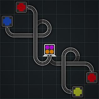
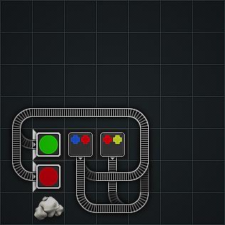
54 Figure A.5: Level 5 Figure A.6: Level 6 Figure A.7: Level 7 Figure A.8: Level 8 Figure A.9: Level 9 Figure A.10: Level 10 49

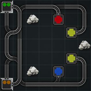
55 Figure A.11: Level 11 Figure A.12: Level 12 Figure A.13: Level 13 Figure A.14: Level 14 Figure A.15: Level 15 Figure A.16: Level 16 50

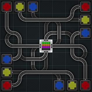
56 Figure A.17: Level 17 Figure A.18: Level 18 Figure A.19: Level 19 Figure A.20: Level 20 Figure A.21: Level 21 Figure A.22: Level 22 51

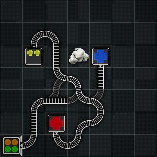
57 Figure A.23: Level 23 Figure A.24: Level 24 Figure A.25: Level 25 Figure A.26: Level 26 Figure A.27: Level 27 Figure A.28: Level 28 52

58 Figure A.29: Level 29 Figure A.30: Level 30 53

59 LevelNr Rating Playing Time Tracks Switches Steps LevelNr Roads Drawn Roads Erased Switches Swapped Table A.1: Average results from the pilot study 54

60 Appendix B Generated levels Figure B.1: Level 1 Figure B.2: Level 2 Figure B.3: Level 3 Figure B.4: Level 4 55

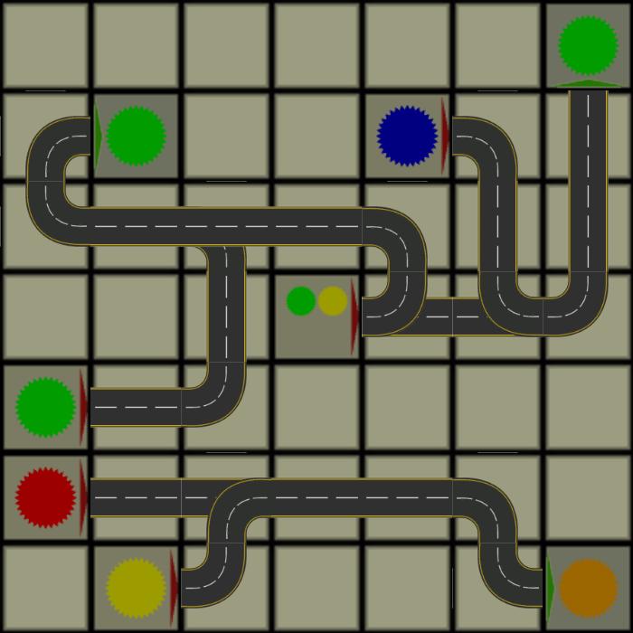
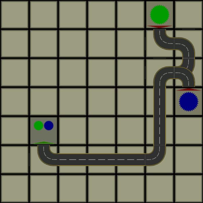
61 Figure B.5: Level 5 Figure B.6: Level 6 Figure B.7: Level 7 Figure B.8: Level 8 Figure B.9: Level 9 Figure B.10: Level 10 56

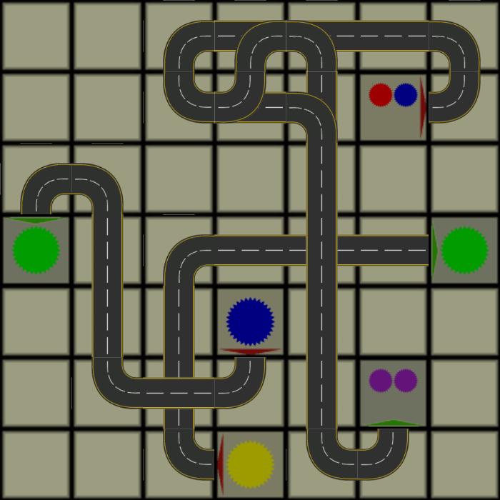
62 Figure B.11: Level 11 Figure B.12: Level 12 Figure B.13: Level 13 Figure B.14: Level 14 Figure B.15: Level 15 Figure B.16: Level 16 57

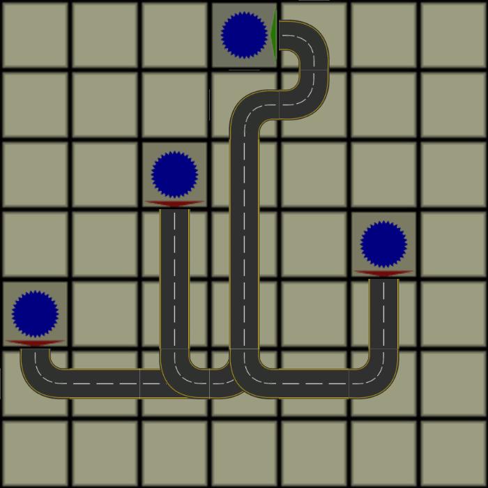
63 Figure B.17: Level 17 Figure B.18: Level 18 Figure B.19: Level 19 Figure B.20: Level 20 Figure B.21: Level 21 Figure B.22: Level 22 58

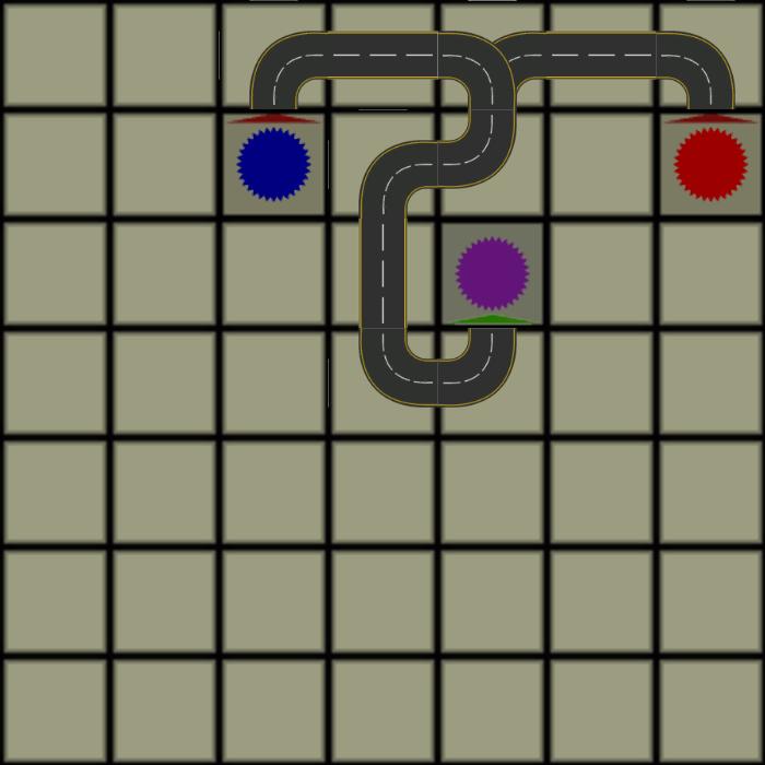
64 Figure B.23: Level 23 Figure B.24: Level 24 Figure B.25: Level 25 Figure B.26: Level 26 59