Localization of Wireless Sensor Networks using Mobile Anchor Nodes

Transcription

1 Localization of Wireless Sensor Networks using Mobile Anchor Nodes Izanoordina Ahmad MSc Mechatronics (Signal and Systems) A thesis submitted for the degree of Doctor of Philosophy at The University of Queensland in 2018 School of Information Technology and Electrical Engineering

2 Abstract Wireless sensor networks (WSNs) are an important class of pervasive computing environments. WSNs have been described as a new instrument for gathering data about the natural world, extending the reach of our human senses. WSN applications are dominated by constrained resources such as energy, computing power, storage and communications bandwidth. An important aspect of WSN operation is the geolocation of all the sensor nodes. Automatically determining sensor position after deployment will improve the reporting of the origin of events in indoor and outdoor applications, in areas such as environmental monitoring, target tracking and disaster relief operations. This thesis explores the use of a mobile anchor moving through a sensor field to localize the nodes in an outdoor setting. The scope of possible experiments with mobile anchor nodes for localization is almost endless. A motivating scenario of air-dropped sensors, and an airborne mobile anchor node will be used to define a focussed set of experiments that have a real application outcome while still providing useful information for other scenarios. With regards to the previous work done by others, little attention has been paid in the literature to how many beacon packets need to be sent by the mobile anchor node, what type of localization algorithm gives the best performance, what path the mobile anchor node should take, what are the geometric parameters of the path, and whether adding range-estimates between blind nodes is beneficial. In answering these questions, this thesis makes several contributions. Firstly, a new algorithm called Volume-based Probabilistic Multi-Lateration (VPML) is devised which can reduce localization errors by up to 75%. Secondly, a simulation framework is devised which can answer questions such as the most suitable flight-path for a mobile anchor. The contributions obtained from the simulation results extend beyond just the VPML algorithm, and include findings about the best beacon placements. Results show that by having well-placed anchors, a low ranging uncertainty can be achieved with fewer anchors and a shorter travel distance. Thirdly, the new algorithm (VPML) together with an optimized flight path (alternate 10m/13m height square grid, 10m spacing) is able to localize air-dropped sensor nodes within a few metres using inherently inaccurate RSSI-based range estimates from the mobile beacon. Finally, a technique for cooperative localization is identified which can reduce the flight path by 80% while still maintaining acceptable localization accuracy. This technique allows decisions to be made about operational requirements for the use of a mobile anchor prior to deployment. i

3 Declaration by author This thesis is composed of my original work, and contains no material previously published or written by another person except where due reference has been made in the text. I have clearly stated the contribution by others to jointly-authored works that I have included in my thesis. I have clearly stated the contribution of others to my thesis as a whole, including statistical assistance, survey design, data analysis, significant technical procedures, professional editorial advice, financial support and any other original research work used or reported in my thesis. The content of my thesis is the result of work I have carried out since the commencement of my higher degree by research candidature and does not include a substantial part of work that has been submitted to qualify for the award of any other degree or diploma in any university or other tertiary institution. I have clearly stated which parts of my thesis, if any, have been submitted to qualify for another award. I acknowledge that an electronic copy of my thesis must be lodged with the University Library and, subject to the policy and procedures of The University of Queensland, the thesis be made available for research and study in accordance with the Copyright Act 1968 unless a period of embargo has been approved by the Dean of the Graduate School. I acknowledge that copyright of all material contained in my thesis resides with the copyright holder(s) of that material. Where appropriate I have obtained copyright permission from the copyright holder to reproduce material in this thesis and have sought permission from co-authors for any jointly authored works included in the thesis. ii

4 Publications during candidature Peer Reviewed Conference Papers I. Ahmad, N. Bergmann, R. Jurdak, and B. Kusy, "Experiments on localization of wireless sensors using airborne mobile anchors," in IEEE Conference on Wireless Sensors (ICWiSe), pp. 1-6: IEEE. 2015, DOI: /ICWISE I. Ahmad, N. W. Bergmann, R. Jurdak, and B. Kusy, "Towards probabilistic localization using airborne mobile anchors," in IEEE International Conference on Pervasive Computing and Communication Workshops (PerCom Workshops), pp. 1-4: IEEE. 2016, DOI: /PERCOMW I. Ahmad, "Localization of wireless sensor networks using a mobile beacon," in IEEE International Conference on Pervasive Computing and Communication Workshops (PerCom Workshops), pp. 1-4: IEEE. 2016, DOI: /PERCOMW Publications included in this thesis No publications included. iii

5 Contributions by others to the thesis No contributions by others. Statement of parts of the thesis submitted to qualify for the award of another degree None. Research Involving Human or Animal Subjects No animal or human participants were involved in this research. iv

6 Acknowledgements My complex, yet exciting journey as a PhD student would not have been possible without the support and assistance from certain special individuals and parties. I would first like to express my greatest gratitude to my dedicated supervisors, Professor Neil Bergmann, Professor Raja Jurdak and Dr. Branislav Kusy for their valuable guidance and patience in helping me throughout the process of researching and writing of this thesis. I could not have asked for better supervisors and mentors to assist me with my PhD program. A big thank you to my sponsorship, MARA (Majlis Amanah Rakyat) and UniKL (Universiti Kuala Lumpur). With their care and financial assistance, I am able to make it this far in the program and is able to reach my goal as a doctoral student. I would also like to extend my special thanks to the research group and colleagues from CSIRO and University of Queensland, Australia for their incredible collaboration, and for always being there when I needed any help. Most importantly, I wish to present my wholeheartedly appreciation to my supportive husband, Saiful Rizal Shafie, my beloved children, Syahmi, Shasmeen, Iris and Iman, my late parents especially my mom, my parents-in-law and my family members. They have not only been supporting and encouraging me to do my best, but have been there every step of the way. Without them, I would not be who I am today. v

7 Financial support Scholarship support from MARA (Majlis Amanah Rakyat) and UniKL (Universiti Kuala Lumpur) in Malaysia is gratefully acknowledged. Financial assistance for attendance at conferences from School of ITEE, University of Queensland, and from CSIRO/Data61 is also gratefully acknowledged. vi

8 Keywords Localization, wireless sensor networks, multilateration, geometric sensitivity, cooperative localization. Australian and New Zealand Standard Research Classifications (ANZSRC) ANZSRC code: , Ubiquitous Computing, 50% ANZSRC code: , Information Engineering and Theory, 50% Fields of Research (FoR) Classification FoR code: 0805, Distributed Computing, 50% FoR code: 0806, Information Systems, 50% vii

9 Table of Contents Abstract... i Declaration by author... ii Publications during candidature... iii Publications included in this thesis... iii Contributions by others to the thesis... iv Statement of parts of the thesis submitted to qualify for the award of another degree... iv Research Involving Human or Animal Subjects... iv Acknowledgements... v Financial support... vi Keywords... vii Australian and New Zealand Standard Research Classifications (ANZSRC)... vii Fields of Research (FoR) Classification... vii List of Figures... xiv List of Tables... xvii List of Abbreviations... xix CHAPTER INTRODUCTION Localization: terminology Motivation Organization of the manuscript CHAPTER LITERATURE REVIEW Distance-based Wireless Localization Techniques Previous Work with Airborne Anchors Range-free localization Centroid system Distance Vector (DV Hop) viii

10 Hop Terrain Appropriate Point in Triangulation (APIT) Range-based algorithms Ranging signals Time of Arrival (ToA) Time Difference of Arrival (TDoA) Received Signal Strength Indicator (RSSI) RF propagation models, advantages and disadvantages Probability distribution using Log normal shadowing model RSSI and its relationship to distance Angle of Arrival (AoA) Angle with range-based localization (Hybrid system) Implementation of GPS-based localization on mobile anchor node Multilateration algorithm for localization Deterministic and Probabilistic Multilateration Gradient descent solution of multilateration Beacon geometric sensitivity and its placement Flip ambiguity Indoor versus outdoor localization Centralized and distributed computation Static anchor node versus mobile anchor node Path planning for the mobile anchor node Random trajectories Dynamic trajectories Static trajectories Cooperative localization using inter blind node range measurement Comparison between non-cooperative and cooperative localization Implementation of cooperative localization ix

11 2.12 Localization performance evaluation Accuracy and localization error Communication and computational cost Number of anchor nodes Energy efficiency Summary CHAPTER RESEARCH QUESTIONS Gap analysis Research questions and methodologies Preliminary experiment RQ1: How does the localization performance of a mobile anchor vary with different numbers of beacon packets, and how does it compare with the use of fixed anchors, or combinations of fixed and mobile anchors? Framework RQ2: What is the localization performance of probabilistic localization algorithms compared to deterministic algorithms, and how does this vary with the number of beacon packets? Framework RQ3: How does the mobile anchor s trajectory influence the performance and what is the most suitable trajectory based on the proposed scenario? How does performance vary with the number of beacons sent and the positions that they are sent from? Framework RQ4: What is the relative localization performance of adding inter-blind node range estimates to anchor range estimates? Framework Summary CHAPTER PRELIMINARY EXPERIMENTS FOR PROPAGATION MODEL x

12 4.1 Radio parameters through preliminary real outdoor experiment Path loss mean Standard Deviation CHAPTER LOCALIZATION ACCURACY VERSUS THE NUMBER OF MOBILE ANCHOR POSITIONS Deterministic Multilateration (DML) Experimental setup Results Localization of the blind node using random mobile anchor node positions Localization of the blind node using designated flight path Localization of the blind node using fixed static anchors Localization of the blind node using a combination of fixed and mobile anchor node Comparison of RSSI variabilities for fixed, mobile and combination anchor Localization of the blind node at poor geometrical position Analysis CHAPTER PROBABILISTIC MULTILATERATION Probabilistic localization algorithms Linear Probabilistic Multilateration (LPML) Volume Probabilistic Multilateration (VPML) Experimental setup Results Localization single blind node localization at favourable and poor geometrical position using DML and VPML Localization for single blind node localization using DML, LPML and VPML DML versus LPML and VPML for low RSSI variability xi

13 DML versus LPML and VPML for medium RSSI variability DML versus LPML and VPML for high RSSI variability Analysis CHAPTER GEOMETRIC SENSITIVITY AND TRAJECTORY OF MOBILE ANCHOR NODE Introduction Experimental Setup Methodology Results Experimental Setup Methodology Results Experimental Setup Methodology Results Experimental Setup Methodology Results Experimental Setup Methodology Results Conclusions CHAPTER COOPERATIVE LOCALIZATION Inter-node cooperative localization algorithm Wide Spacing Cooperation Localization Experimental Setup Results Varying Node Density xii

14 8.2.3 Results using 60m spacing Changing Minimum Number of Anchors Edge-Based Cooperative Localization Experimental Setup Results for 200 Blind Nodes Results for 1000 Blind Nodes Analysis CHAPTER CONCLUSION, CONTRIBUTIONS AND FUTURE WORK Research Question 1 (Localization accuracy vs. number of mobile anchor positions) Research Question 2 (Probabilistic Multilateration) Research Question 3 (Geometric sensitivity and trajectory of mobile anchor node) Research Question 4 (Cooperative localization) Original Contributions Future Research References Appendix A Appendix B Appendix C Appendix D Appendix E Appendix F xiii

15 List of Figures Figure 1.1: Localization using mobile anchor node Figure 2.1: Localization process... 7 Figure 2.2: Wireless localization techniques Figure 2.3: Multilateration using TDoA and ToA measurements with hyperbolae and circle respectively as possible emitter location Figure 2.4: Log normal distribution of distances for packets with RSSI= Figure 2.5: Intersection points of spheres in Multilateration Figure 2.6: Flip ambiguities Figure 2.7: Signal fingerprinting work by collecting the RSSI values from multiple WiFi access points or base stations to generate a unique signature of an area Figure 2.8: Static path planning for (a) Scan (b) Hilbert (c) Circle and (d) S-Curves with individual path length Figure 2.9: Non-Cooperative localization Figure 2.10: Cooperative localization Figure 2.11: Localization of wireless sensor networks using mobile anchor nodes Figure 4.1: Camazotz prototype device without battery and solar panel Figure 4.2: Path Loss mean versus logarithm of distance Figure 4.3: Histogram and log-normal shadowing distribution of the reading at 20 metres Figure 5.1: The actual and estimated blind node s location on the ground with designated position of anchor node Figure 5.2: Localization error versus number of mobile anchor node with random positions for blind node deployed on the ground Figure 5.3: Average localization error in metres for 15 mobile anchors with designated flightpath positions for different RSSI variability Figure 5.4: Localization error using four fixed anchors only for blind node at 25,25, Figure 5.5: Localization error using four fixed anchors only for blind node at 40, 25, Figure 5.6: Localization of fixed blind node on the ground using combination of fixed anchor and designated position of mobile anchor node Figure 5.7: Comparison of 4 fixed anchors, the best 4 to 15 mobile anchor node positions and the best 4 to 15 combination of fixed and mobile anchor positions with low variability Figure 5.8: Comparison of 4 fixed anchors, the best 4 to 15 mobile anchor node positions and the best 4 to 15 combination of fixed and mobile anchor positions with medium variability xiv

16 Figure 5.9: Comparison of 4 fixed anchors, the best 4 to 15 mobile anchor node positions and the best 4 to 15 combination of fixed and mobile anchor positions with high variability Figure 5.10: Localization of fixed blind node at poor geometrical position using fixed anchor and designated position of mobile anchor node Figure 6.1: 3 dimensional spatial PDF Figure 6.2: Comparison between DML and VPML Figure 6.3: Comparison between LPML and VPML Figure 6.4: Median localization error using N from 15 designated mobile anchor node positions with DML and VPML for node in favourable position. 10/90 percentile ranges also shown Figure 6.5: Median localization error using N from 15 designated mobile anchor node positions with DML and VPML for node in unfavourable position. 10/90 percentile ranges shown Figure 6.6: DML versus LPML and VPML for standard deviation of 1dB Figure 6.7: DML versus LPML and VPML for standard deviation of 3.36dB Figure 6.8: DML versus LPML and VPML for standard deviation of 5dB Figure 7.1: Median error (m) versus number of iterations for 5 trials Figure 7.2: Comparison between height for blind node 127,192,0 and 500,500, Figure 7.3: Square grid path with 5m beacon spacing and alternate layers of 10m and 11m height 90 Figure 7.4: Square grid path with 30m beacon spacing and laternate layers of 10m and 13m height Figure 7.5: Comparison between localization errors versus beacon distance interval using 20 beacons Figure 7.6: Comparison of average localization error between size for blind node 5 (500,500,0) Figure 7.7: Comparison of average localization error between size for blind node (0,0,0) Figure 7.8: Comparison of average localization error between size for blind node (142, 439, 0) Figure 7.9: Anchor positions according to the strongest RSSI based on 5 metre spacing Figure 7.10: Anchor positions according to the strongest RSSI based on 10 metre spacing Figure 7.11: Anchor positions according to the strongest RSSI based on 20 metre spacing Figure 8.1: Localization using 50 metres spaces between beacons in square grid path for a) 50 b) 100 and c) 200 blind nodes Figure 8.2: Median localization error for 50 blind nodes based on generation Figure 8.3: Localized and unlocalized (UL) nodes through generation (G1-G2) for 50 blind nodes Figure 8.4: Average localization error for 100 blind nodes based on generation xv

17 Figure 8.5: Localized and unlocalized (UL) nodes through generation (G1-G2) for 100 blind nodes Figure 8.6: Average localization error for 200 blind nodes based on generation Figure 8.7: Localized and unlocalized (UL) nodes through generation (G1-G2) for 200 blind nodes Figure 8.8: Average localization error for 200 blind node based on generation using 60 metre spaces Figure 8.9: Localized and unlocalized (UL) nodes through generation (G1-G2) for 200 blind nodes using 60 metres spaces Figure 8.10: Average localization error for 200 blind nodes based on generation using (a) 6, (b) 7 and (c) 8 minimum anchor positions Figure 8.11: Local anchors for each generation (G1 to G3) using 7 anchor positions Figure 8.12: Local anchors for each generation (G1 to G3) using 8 anchor positions Figure 8.13: Localization using 50 metres spacing between beacons using 200 blind nodes and edge path planning Figure 8.14: Localization error for 200 blind nodes based on generation using edge path panning 124 Figure 8.15: Localized and unlocalized (UL) nodes through generation (G1-G2) for 200 blind nodes using edge path planning Figure 8.16: Localization for 1000 blind nodes using edge path planning Figure 8.17: Localized blind nodes through generation (G1-G4) for 200 blind nodes using edge path planning xvi

18 List of Tables Table 2.1: Previous works with Airborne anchors... 9 Table 4.1: Path loss mean for each distance Table 4.2: Standard Deviation Table 4.3: Parameters for simulation Table 5.1: Average localization error in metres for 15 mobile anchors with random positions for different RSSI variability Table 5.2: Localization error for 15 designated mobile anchor node at different RSSI variability Table 5.3: Localization error using four fixed anchors for blind node 25,25, Table 5.4: Localization error using four fixed anchors for blind node 40,25, Table 5.5: Localization error for 15 anchors at different RSSI variability Table 5.6: New position of anchor nodes (fixed and mobile anchor) based on the shortest estimated distance in metre Table 5.7: Localization accuracy for different scenario with low variability Table 5.8: Localization accuracy for different scenario with medium variability Table 5.9: Localization accuracy for different scenario with high variability Table 5.10: Localization accuracy for blind node at poor geometrical position Table 6.1: Localization median error (metres) and standard deviation (metres) for favourable blind node position Table 6.2: Localization median error (metres) and standard deviation (metres) for unfavourable blind node position Table 6.3: The median error and standard deviations (SD) of errors (in metres) for DML, LPML and VPML for standard deviation of 1 db Table 6.4: The median error and standard deviations (SD) of errors (in metres) for DML, LPML and VPML for standard deviation of 3.36dB Table 6.5: The median error and standard deviations (SD) of errors (in metres) for DML, LPML and VPML for standard deviation of 5dB Table 7.1: Position of 25 blind nodes (in metres) Table 7.2: Median errors (m) for each of 5 trials Table 7.3: Average localization error for blind node 127, 192, 0 and 500, 500, Table 7.4: Comparison of average localization error with 20 beacons based on beacon distance interval and height Table 7.5: Comparison of average localization error between size for blind node 5 (500,500,0) xvii

19 Table 7.6: Comparison of average localization error between size for blind node (0,0,0) Table 7.7: Comparison of average localization error between size for blind node (142,439,0) Table 7.8: Path characteristics for different grid spacing Table 7.9: Anchor positions according to the strongest RSSI based on 5 metre spacing Table 7.10: Anchor positions according to the strongest RSSI based on 10 metre spacing Table 7.11: Anchor positions according to the strongest RSSI based on 20 metre spacing Table 7.12: Angle between beacons for 5m spacing Table 7.13: Angle between beacons for 10m spacing Table 7.14: Angle between beacons for 20m spacing Table 8.1: Positions of mobile anchor for square grid path Table 8.2: Local and mobile anchor for localized blind node 13 and 42 by using 200 blind nodes 115 Table 8.3: Performance versus Node Density Table 8.4: Localization Errors versus Minimum Anchors Table 8.5: Position of mobile anchor node for edge path xviii

20 List of Abbreviations 2D 3D 3D-ADAL AGPS AoA APIT COLA CRLB dbm DGPS DML DREAMS DV ECG FLS GDM GDOP GPS HPSO IMU IoT LMAT LNMS LoS LPML Two Dimensions Three Dimensions Three-Dimensional Azimuthally Defined Area Localization Assisted GPS Angle of Arrival Appropriate Point in Triangulation Complexity-Reduced 3D Trilateration Localization Approach Cramer Rao Low Bound decibels referenced to 1mW power Differential GPS Deterministic Multilateration Deterministic beacon Mobility Scheduling Distance Vector Electrocardiogram Fuzzy Logic System Gradient descent method Geometric Dilution of Precision Global Positioning System Hybrid-Particle Swarm Optimisation Inertial Measurement Unit Internet of Things Mobile Anchor node based on Trilateration Log Normal Shadowing Model Line of Sight Linear Probabilistic Multilateration xix

21 LS MAALRH MAE MBAL ML MRS N NLOS PDF PS ReNLoc RF RMSE RSSI SBLS SMAL TDoA ToA ToF UAV UGV VPML WiFi WSNs Least square Mobile Anchor Assisted Localization Algorithm based on Regular Hexagon Mean Absolute Error Mobile anchor node Assisted Localization Maximum Likelihood Multirobot System Number Non-line of sight Probability Distribution Function Push-sum Relaid Ranging Localization Radio Frequency Root Mean Square Error Received Signal Strength Indicator Sound-Based Localization System Single Mobile Anchor Location Time Difference of Arrival Time of Arrival Time of Flight Unmanned Aerial Vehicle Utility Ground Vehicle Volume Probabilistic Multilateration Wireless Fidelity Wireless sensor networks xx

22 CHAPTER 1 INTRODUCTION Wireless sensor networks (WSNs) are an important class of pervasive computing environments. As one of the important technologies in the Internet of Things (IoT), WSNs have been described as a new instrument for gathering data about the natural world, extending the reach of our human senses. WSNs are composed of intercommunicating networks of smart sensor nodes, they are deployed in real environments and usually they are small, low-cost devices with limited processing capabilities. The applications of WSN are enormous, such as in military, civil and environmental applications [1]. In environmental monitoring, the sensors can detect scalar features like temperature or multimedia features like audio and video. WSNs can be used to detect bushfires, to track the movements of animals to observe their habits, to observe plant growth, or to monitor soil movement. In traffic control systems, sensors are used to monitor vehicle movements. In industrial monitoring, sensors can be used to monitor a production line, to reduce downtime. Medical sensors are used to monitor the condition of patients such as their blood pressure, blood sugar level, or electrocardiogram (ECG). These sensors often simply store and forward the information for subsequent data analysis. WSN applications are dominated by constrained resources such as energy, computing power, storage and communications bandwidth [2]. The issues of hardware and operating system, deployment, wireless sensors and actuators, time synchronization and localization can affect the design and performance of the overall network. In some cases, sensors are deployed in remote areas without significant communications infrastructure. For example, sensors could be dropped in a forest to monitor the progress of a bushfire. Another useful example from our laboratory is in Springbrook rainforest where a long term WSNbased monitoring system has been deployed to monitor forest regrowth after previous logging in the area, to better understand how forests regenerate [3]. In cases where sensors are remotely deployed, automatically determining the precise geolocation of sensor nodes after deployment is often critical for the reporting of origin of events in indoor and outdoor applications. For instance, without the precise location of temperature readings in a forest, the location of a bushfire cannot be detected. To date, many algorithms have been proposed to solve the issues of device localization. Many of the algorithms that have been published are suitable for specific scenarios, such as indoor localization of mobile phones or outdoor localization with using a small number of geo-located anchor nodes. Additionally, some localization technologies such as the 1

23 Global Positioning System (GPS) are relatively expensive and not always available. Factors of energy consumption, communication cost and require location accuracy also need to be considered while choosing an appropriate localization algorithm. 1.1 Localization: terminology. Many different objects need to be localized in many different situations. For instance, a tennis player uses stereo vision to localize the position of the ball to return a shot and an airport uses radar to localize planes in its airspace. Other examples are a car navigation system that localizes its position relative to a stored map, a tracker dog that follows a scent trail to find the location of a fugitive, and a bat that uses sonar to find the location of its insect prey. All these methods use different sources of information and different computation algorithms. My research concentrates on one very narrow field of localization, which is the localization of wireless sensor nodes, which determine their position based on wireless communications with other nodes with known position. The following terms are used throughout this thesis; 1. An anchor node is a node with known position, which acts as a location reference node and transmits beacon packets, which include its current position. An anchor node may be fixed or mobile. 2. A mobile anchor node is a moving anchor node, which traverses over the deployment region, regularly transmitting beacon packets. 3. A blind node is a node with unknown location within the deployment region. It uses information in multiple beacon packets to estimate its location. 4. A static node is a node whose position remain unchanged after the deployment. In this research, all blind nodes are static nodes. 5. A local anchor is initially a blind node. After it has been localized, it acts as an anchor node for other blind nodes. 1.2 Motivation. This research considers a motivating scenario where the sensor nodes are carried by an aircraft and are then dropped and randomly scattered within the sensing region such as in the application of bushfire monitoring [3]. In this scenario, these nodes are not guaranteed to land at particular locations or in particular orientations. They might be on the ground or at some non-zero elevation, e.g. in a tree. The nodes should be lightweight and rugged enough to minimize the possibility of being damaged 2

24 during their deployment [4]. When a sensor is deployed in the sensing region, its sensor data is often of limited use unless the position of the sensor is known when the measurement was taken. While localization technologies like GPS are now relatively cheap, the additional circuitry, antennas, energy use and computational resources are not always suitable for low cost, low-energy sensors, especially where the sensor is static and only needs to be localized once. Additionally, GPS is not always available due to occlusion by buildings, trees or other obstructions. While it would be technically possible to add GPS on each node for accurate localization, it is not cost effective for very low-cost nodes. Instead, localization can be achieved by using the same aircraft to act as a mobile anchor. The aircraft can be equipped with GPS and can broadcast its position at regular intervals along a specific trajectory. The deployed sensor nodes are blind nodes [5]. The motivating scenario for this thesis is shown in figure 1.1. An aircraft carrying air-dropped sensor nodes travels along a specific path while distributing the nodes. These nodes are randomly scattered within the sensing region, and need to be subsequently located. The same aircraft is then used as a mobile anchor sending beacon messages to localize the nodes. The aim of the thesis is to investigate localization techniques which can reduce the localization error during this phase, and which can also determine a good trajectory which trades off adequate localisation accuracy with reasonable travel distance. Figure 1.1: Localization using mobile anchor node. Adapted with permission from [4]. One focus of this thesis is examining how to achieve the best localization performance in this scenario, viz. randomly deployed nodes localized with an airborne mobile anchor, sending beacon 3

25 packets. Particular issues that are addressed are the impact on localization error of factors such as random or planned positions of mobile anchor nodes, the number of mobile anchor node positions used, and the variability of Received Signal Strength Indicator (RSSI) range measurements. One key aspect investigates whether a designated flight path is better than random anchor positions, and how localization error changes with RSSI variability. Does adding a few ground based anchors equipped with GPS improve the localization? The research also examines the number of beacon messages that are needed for the best localization accuracy. Multilateration is a common localization algorithm that can be applied when sufficient beacon messages from different mobile anchor node positions are received by a blind node. The most commonly used multilateration algorithm known as Deterministic Multilateration (DML) will be compared to an existing probabilistic algorithm referred to here as Linear Probabilistic Multilateration (LPML), as well as an improved algorithm developed in this thesis called Volume Probabilistic Multilateration (VPML). The thesis presents a detailed description of this new RSSI-based localization algorithm, which uses a volumetric probability distribution function to find the most likely position of a node by information fusion from multiple mobile anchor node radio packets. MATLAB simulations are used to compare the multilateration approaches over a range of different localization scenarios. Generally, RSSI is an inaccurate distance estimator [6], and errors in distance estimation are worse for larger distances. The accuracy of the multilateration localization also depends on the geometry of the anchor positions, and for this air-dropped scenario, the geometry is not ideal, since all the anchor positions are in the same half plane above the blind nodes. Normally, one would expect that using more distance estimates would improve the accuracy of localization, but this is not obviously the case here, as our experiments will show. The large errors associated with estimates of distance from low RSSI values means that using all available readings may degrade performance. The optimal mobile anchor path for good localization is also an open question. This research investigates the effect of the flight path and the number of beacon packets on accuracy. Not all nodes might be localized by mobile anchor beacons. In this case, those nodes that have already been localized can act as local anchors for the unlocalized blind nodes. This research also investigates this cooperative localization. Overall, the thesis contributions are as follows. A new algorithm called VPML is developed which significantly reduces localization error. Furthermore, the design of the most suitable flightpath for a mobile anchor is investigated. The thesis demonstrates a trade-off between the energy costs of travelling and beacon transmission versus the localization accuracy. The combination of VPML 4

26 algorithm with this optimized flight path is able to localize air-dropped sensor using inaccurate RSSI from the mobile anchor. Finally, cooperative localization with the VPML algorithm is demonstrated as a solution for reducing the flight path while maintaining acceptable localization accuracy. 1.3 Organization of the manuscript. The rest of the thesis is organized as follows. Chapter 2 provides a literature review and survey of localization in wireless sensor networks. Chapter 3 defines the research questions and the general framework for answering them. A preliminary experiment to validate the simulations will be undertaken in Chapter 4. Chapter 5 investigates deterministic multilateration performance. Probabilistic algorithms will be discussed in chapter 6 to validate the performance of our new algorithm compared to the previous work. Explorations of geometric sensitivity, appropriate path planning in in Chapter 7 and cooperative localization is in Chapter 8. Finally, the conclusions and future work are presented in chapter 9. 5

27 CHAPTER 2 LITERATURE REVIEW Localization involves finding the position of an item in space. Localization can be twodimensional (2D), such as finding position on a map, or it can be three dimensional (3D), such as finding height as well as latitude and longitude. Localization can also be 4D, if the localization involves tracking the positions of a moving object through time. This thesis deals with 3D localization of static items, in this case WSN nodes, using a mobile anchor, in this case this is assumed to be an unmanned aerial vehicle (UAV). Localization can be done with many different sensors in many different applications. For example, an airport uses radar to localize aircraft that are nearby, a fishing boat may use sonar to localize a school of fish, and a car s parking sensors use ultrasonics to localize nearby obstacles. Because localization is such a broad topic, this review concentrates only on techniques that are relevant to WSNs, and only those that use radio-frequency signals. Section 2.1 reviews WSN localization techniques that depend on estimating the distance or range of blind nodes from localization anchors. This section includes a review of different methods for estimating range, as well as methods for using that range for localization. Section 2.2 deals with WSN localization techniques that use estimates of angles to anchors. Section 2.3 investigates the use of the Global Positioning System (GPS) for WSN localization. Section 2.4 explores in more detail the multilateration technique, which is the basis of the algorithms in this thesis. Section 2.5 describes gradient descent, which is a convex optimization technique that is used to find the best position estimate in techniques like multilateration. Section 2.6 looks at the dependence of localization accuracy on the position of the anchor nodes, and describes flip ambiguity which is a potential problem in this work. Section 2.7 compares WSN localization techniques for indoor and outdoor localization, which have quite different challenges. Section 2.8 looks at where in the WSN system localization computations could executed either on the nodes or centrally. Section 2.9 describes differences between localization from static anchors and from mobile anchors, and section 2.10 reviews previous work on path panning for mobile anchors. Section 2.11 summarises work on cooperative localization, where newly localized nodes assist nearby blind nodes. Section 2.12 describes methods and metrics for measuring the accuracy of localization, and section 2.13 looks at energy efficiency, with a final summary in section The review of the 6

28 current state-of-the-art in this chapter will be used to analyse gaps in the research in this area, and to propose the research questions for this thesis in Chapter Distance-based Wireless Localization Techniques. Localization begins with acquiring input data such as the location of the anchor nodes and their estimated ranging signal as in figure 2.1. Based on these inputs, the distance or the angle between the anchor and blind nodes can be determined, and thus the estimated position of the blind nodes can be calculated. Figure 2.1: Localization process Previous Work with Airborne Anchors. Localization is necessary for many indoor and outdoor WSN applications. It provides sampling locations in data collection such as temperature and humidity in environmental monitoring, as well as providing the exact location of events in a forest fire, earthquake or aircraft navigation. In the motivating scenario for this thesis, not all air-dropped nodes are guaranteed to be on a flat ground plane, so 3D localization is needed. Pandya and Patel [7] provide a summary of suitable 3-D localization algorithms, many of which are described in more detail in the following sections. Ou and Ssu describe some previous research in airborne localization [8]. In their work, a rangefree algorithm is implemented on self-localized nodes by utilizing the information transmitted by the flying anchors. Their node positioning is improved by various enhancement strategies such as chord selection and jittered beacon scheduling. The algorithm takes the GPS errors of the anchor into account and it performs reasonably well in terms of localization time and a lower beacon overhead. However, this work used a range-free algorithm, which has a relatively low localization accuracy. Three beacon messages were used by Kumar et. al. [9] to localize a node that has been distributed by a flying anchor equipped with GPS. The algorithm saves computation time and uses few anchors. However, Yadav et. al [10] show that, using more than three beacon messages reduces the 7

29 localization error. Here, the initial work used an algorithm that calculates the position of node individually based on the range-free sphere equation. This work has been improved in [11] by introducing the complexity-reduced 3D lateration localization approach (COLA) using RSSI values of four anchor nodes. Although it has a higher computational cost, the algorithm provides higher location accuracy. A three dimensional flying model based algorithm is also described in [12]. They proposed a Single Mobile Anchor Location (SMAL) algorithm that gave good accuracy. Their research is similar to our scenario because it uses only a single mobile anchor node as the anchor node. Their work was a motivation for and improved algorithm by Abdi and Haghighat [13] to improve the average localization errors and execution times. However, in their scenario, the mobile anchor node is moving using a random path that potential results in longer travel time and less reliable localization due to unplanned trajectories. The previous 3D localization work from airborne anchors focussed on range-free 3D localization. There is less work concerned with the 3D localization using a range-based algorithm for mobile anchors, which should be able to provide substantially better accuracy. Table 2.1 lists the previous work in the airborne mobile anchor area. 8

30 Table 2.1: Previous works with airborne anchors. Authors [ref] Algorithm Accuracy Strengths/Weaknesses Chia-Ho & RSSI +/-1m + Few anchors. Kuo-Feng [8] Range-free -Assumes perfectly predictable Chord selection range. scheme Kumar et. al. [9] Range free using three beacon message Yadav et. al [10] Range free/ Connectivity range +/-1m No error if the beacon message is at the surface of connectivity range +Few anchors. +Reduce computation times. -Random way point/ random direction walk -Trilateration +Reduce overhead +Reduce memory resource Seo & Kim [11] COLA/ RSSI +/-2 to 4m -Trilateration +Reduce computational cost by using a typical trilateration for 3D trilateration Abdi & RSSI +/-1.5m -Only use three neighbour Haghighat [13] Neighbour nodes Scheme/ Anchor + Improve average localization Return Scheme/ error and reduce average Three Nodes location error with steeper Scheme slope 9

31 There are many different schemes for wireless localization, used over many decades for applications as diverse as aircraft navigation or finding a lost mobile phone. The appropriate tools and schemes used in mobile sensor network localization has been compared in [14]. Localization can be grouped into range-free and range-based schemes [15] as shown in figure 2.2. Range-free schemes apply network connectivity to support coarse node position estimation with simple measurements (i.e. in radio range or outside radio range). Range-free approaches include geometric conjecture, Distance Vector (DV) hop, centroid and Appropriate Point in Triangulation (APIT). In contrast, range-based schemes are based on estimates of distance. These schemes require more expensive hardware in their implementation but they ares more accurate than the range-free schemes. The techniques use measurements such as Time of Arrival (ToA), Time Difference of Arrival (TDoA), Angle of Arrival (AoA) and Received Signal Strength Indicator (RSSI) in the algorithm. Among these metrics, RSSI information is available with most modern radio receivers and this makes it practical to be used in many WSNs. Other techniques typically require additional specialised hardware. However, RSSI is not a particularly accurate or stable estimator of distance, and this introduces complexity into RSSI-based localization. Figure 2.2: Wireless localization techniques Range-free localization. A 3D range-free localization has been implemented in [16] by evaluating the coordinates of anchor nodes that form a triangle in a grid system to estimate the position of a blind node. The RSSI is used 10

32 to compare with a threshold value in order to localize the blind node. The results show that the scheme has less error if the anchor nodes are uniformly distributed during the deployment. Blind nodes are localized using in 3D node range-free localization in [17]. Anchor nodes are randomly distributed to localize the randomly distributed target node located at the middle and bottom layer boundaries. The problem of non-linearity between RSSI and distance is solved by using a fuzzy logic system. RSSI information between the two nodes is sufficient for the target nodes to estimate its position. The location of the target node is computed based on the edge weights between the target and neighbouring anchor nodes using a Fuzzy Logic System (FLS). The results have been compared with other range-free algorithms such as Hybrid-Particle Swarm Optimisation (HPSO), centroid and weighted centroid to show that this algorithm has better performance than the other algorithms. From the viewpoint of cost and energy consumption, the range-free algorithm is preferable since it does not require hardware to measure distance or angle. The mobile anchor node with GPS will periodically broadcast a beacon message including its current location. The mobile anchor node is assumed to move in a straight line. The initial work in [8] has been improved in [18] by obtaining possible points through the intersection of three spheres. The position of blind nodes is determined from these intersection points. As a results, the scheme provided higher localization accuracy compared to Ou s scheme in [8]. Additionally, more appropriate path planning is part of their future investigation since the existing path results in poor localization accuracy. A range-free algorithm called three-dimensional azimuthally defined area localization (3D- ADAL), has been proposed in [19]. The estimated position of blind nodes is based on the information received from the mobile anchor node that is equipped with a rotary and tilting directional antenna. The algorithm has the advantages of being simple and produced higher energy efficiency that contributes to the sensor s lifetime. The sensor nodes within the ranges of the mobile anchor node received a beacon messages that depends on the angular velocity of the directional antenna, the time between each transmission and the velocity of the mobile anchor node. The error can be reduced by increasing the number of virtual beacon nodes and by decreasing the beamwidth of the directional antenna. The work needs to be improved in order to accomplish larger distance data communications to the WSN. Range-free localization is based on the radio connectivity between nodes and does not use a distance measurement [20] to infer the location. It does not require any extra range estimation hardware like range-based localization. However, it only provides coarse accuracy. Range-free methods can be classified as centroid system, distance vector (DV), hop terrain, and appropriate point in triangulation (APIT) [1], and these are described in more detail below. 11

33 Centroid system. Bulusu and Heidemann [21] proposed a centroid algorithm that uses anchor beacons with location information to estimate the blind node s position. The multiple anchor nodes will broadcast their positions from their GPS receiver to the blind nodes [22]. The blind node (Xest, Yest) estimates its location using the average of all N beacon positions as follows:,, (2.1) Distance Vector (DV Hop). A DV HOP [23] measures the number of hop counts from each blind node to anchor nodes using the hop count techniques and triangulation. The hop count method is useful to find the hop between the two nodes in isotropic networks. The distance between the hops can be determined using the multiplication of the average per hop. For instance, the anchor will broadcast a beacon throughout the network, which consists of the anchors location and a hop count parameter initialized to one. Each blind node will maintain the minimum counter value per anchor of received beacons and it will ignore those beacons with higher hop-count values. Thus, this mechanism will allow all nodes in the network to get the shortest distance in hops to every anchor. Using the following formula, the average single hop distance estimated by the anchor can be obtained. (2.2) Where,, is the location of anchor j while hj is the distance in hops from anchor j to anchor i. Once the hop size is calculated, the anchors will propagate this information out to the nearby nodes. Finally, the location of the blind nodes can be estimated using a multilateration algorithm. In [24] the improved DV hop algorithm has been proposed to increase the accuracy and produce lower computational complexity. The algorithm is enhanced by adding additional localization information such as the direction of arrival Hop Terrain. The hop terrain algorithm finds the distance between anchor and blind node as follows. The blind node obtains its initial position estimation by using the DV hop algorithm above. Then the initial position estimation is broadcast to the neighbour nodes. The neighbour nodes receive the information that contains estimates of distance information. This algorithm minimizes the least square error between inter-node distances based on the estimated positions and average of inter-hop distance. In 12

34 [25] the performance of Hop Terrain is analysed and they proved that the node is localized up to a bounded error based on average hop distance Appropriate Point in Triangulation (APIT). In the APIT scheme [26], the blind node connects to the anchor nodes to get the position information of anchor nodes and the energy information of received signal energy. Using this algorithm, it chooses 3 nodes among N anchor nodes to test whether the blind node is within the triangle, formed by these 3 anchor nodes. If so, the position of the blind node is determined as the centroid of this area. The main drawback of APIT is it requires more anchor nodes than the average number of anchors in localization [27]. Furthermore, it also does not make any assumption about the correlation between absolute distance and the radio signal strength. Overall, the range-free localization schemes require less information and simpler receivers than range-based localization, however they are less precise. Given that RSSI is now available on almost all WSN radio receivers, no extra complexity in hardware is required to achieve the better accuracy of range-based techniques. The following sections explain these techniques Range-based algorithms. Range-based localization techniques calculate the position of blind nodes through the estimation of distances or angles from anchors, using techniques like triangulation, trilateration, or multilateration. The system can use long-range anchors that transmit over the whole network or it use a short-range beacon that transmits to a local subset of nodes. The work in [28] discusses the various range-based techniques for localization by using the distance or angle, by using the weighted RSSI, by using the geometry of beacons or by using cooperative localization between blind nodes. The geometric arrangement of anchor nodes can be used as a strategy to improve the accuracy. The equilateral triangle of mobile anchor node at proper placement improved the position estimation compared to random placement [29] [30]. The localized blind nodes can be used as new local anchors as in [31] Ranging signals. Audio and radio frequency signals are the common used for ranging. They differ in terms of speed, wavelength and frequency. Radio signals travel at speed of light, approximately a million times faster than audio signals at a few hundred metres per second in air. 13

35 The work in [32] presented the results from three different systems applied in 3D position measurement. Two commercial systems are based on radio frequency measurements while the other employs a time-of-flight measurements based on audible signals in an acoustic prototype system. The experiments focused on the accuracies of the systems, the position update rates, the end-to-end delay as well as the energy consumption. The tests were implemented for indoor localization with stationary measurements at known positions, and with dynamics scenarios on a linear track at given velocities. The Sound-Based Localization System (SBLS) performed well in terms of accuracy and precision of the position. Its low update rate and high latency is suitable for stationary localization. One RF system, Decawave, provided a very high update rate and low delay, making it suitable for the dynamic applications. The other RF system, a Time Domain system, not only provided higher update rates but also lower delay with better accuracy than the Decawave system. When comparing these three systems in cluttered environments, (SBLS, Decawave and Time Domain), the reception of acoustic signals was greatly disturbed by the obstructions thus it led to poor performance for SBLS. This scenario can be dealt with in a better way by using the RF based systems. The following sub section will discusses the most common range measurement techniques Time of Arrival (ToA). This technique uses the propagation time between signal transmission and reception, plus the transmission speed of the medium to estimate distance. This approach is commonly used for acoustic ranging. However, the technique needs very high clock accuracy and time synchronization for use with RF, and is not practical with WSN-grade technology [33]. In ToA, the time of emission can be included in the beacon and received by the time-synchronized sensors [34], or it can be at known times. Once the features of the signal are obtained, ToA measurements are compared to the transmission time. Here the beacon transmitted by the anchor consists of the anchor positions and the time of transmission. Given a formula for ToA; Time of Flight (ToF) = (time of reception - time of transmission) (2.3) Therefore, the range estimate can be calculated using the following formula. Range = ToF / Propagation speed (2.4) Time Difference of Arrival (TDoA). In TDoA, the unknown time of emission is eliminated by calculating the difference between arrivals of one signal at two receivers. The blind node sends a message (at unknown time) and 14

36 synchronised anchors will record the arrival times to give TDOA. This requires very high synchronization between transmitters (anchors) but does not requires transmitter-receiver synchronization. It has been used in aircraft navigation, with expensive base stations. Localization in TDoA (shown as the red curve) is referred as hyperbolic positioning whereby the emitter position on a hyperboloid is localized with the two sensors as foci as shown in figure 2.3. Figure 2.3: Multilateration using TDoA and ToA measurements with hyperbolae and circles respectively as possible emitter location. Adapted with permission from [34]. The measurements of TDoA is obtained by calculating the difference between two ToA measurements and the unknown time of emission will be eliminated. There should be a pair of sensors to get the measurements. The most common methods used for TDoA is the generalized cross correlation method. The cross correlation function between two signals received from two receivers is given by integrating the lag product of two received signals for a sufficient time period [35] Received Signal Strength Indicator (RSSI). Received Signal Strength Indicator (RSSI) is a measurement of the RF power received at the receiver. Assuming known transmit power, receiver antenna gains, and signal path loss as a function of distance, RSSI can be used to estimate transmit distance. RSSI is calculated from the antenna voltage being measured at the receiver and is indicated as a measured power. RSSI ranging calculates the propagation loss and transforms the value into the distance, using an experimental or theoretical signal path loss model. The signal strength is influenced 15

37 by at least three environmental factors such as the node elevation from the ground, transmission power while collecting the data and the position of the antenna [36]. In [37], the localization of the deployed blind nodes uses RSSI as a range estimation technique. As suggested by the commonly used log-normal shadowing model for Radio Frequency (RF) propagation, RSSI is a random variable based on distance. Therefore, the estimate of ranging distance using RSSI is also a random variable. It is also known as an inaccurate distance estimator [6], and errors in distance estimation are worse for larger distances. RSSI ranging is explored in detail in Chapter RF propagation models, advantages and disadvantages. Line Of Sight (LOS) is where the transmit and receive stations are in view of each other without any sort of an obstacle between them. Point-to-point microwave links and satellite transmission are examples of line-of-sight communication. RSSI measurements are sensitive to multipath, diffraction, fading and non LOS measurement. RSSI is difficult to use as a range estimator in cluttered or indoor environments. RSSI can be modelled with a Free Space propagation model, Two-Ray ground model, and with a Log Normal Shadowing Model (LNMS). Among these categories, LNMS is the most common signal propagation model and does not have any special requirements for the application environment [38]. a) Free space propagation model. This model is used when the transmitter and receiver have clear LOS between them, thus the RSS can be predicted and is given by the Friss free equation. Pr (d) = (Pt. Gt. Gr. 2 ) / (4 ) 2. d 2. L (2.5) where Pt is transmitted power, Pr (d) is received power, Gt is transmitter antenna gain, Gr is the receiver antenna gain, D is the transmitter to receiver separation distance (m), L is system loss factor and is the wavelength in metres. For a given transmitter and receiver configuration, Pt,Gt,Gr, and are all constant, so the relationship can be more easily be seen. b) Two-ray ground model. This model considers the path between the transmitter and receiver consists of two rays: the direct ray and a ground reflected ray. The two rays destructively interfere (reflected ray is opposite in phase after reflection) and as distance (d) increases the relative phase difference decreases between LOS and reflected wave. Thus, the attenuation is more rapid than the free-space model. 16

38 Pr (d) = (Pt. Gt. Gr. (ht 2 hr 2 )) / d 4 (2.6) where ht is the transmitter antenna height and hr is the receiver antenna height. c) Log Normal Shadowing Model. Since RSSI measurement is readily available, it has become a popular topic in localization research. Its unpredictable performance can be considered as being due to Gaussian noise, and this fits with the existing log normal shadowing model for noisy communication paths. The major variability of RSSI is due to extrinsic and intrinsic factors, i.e. factors about the environment and factors about the device. In extrinsic factors, error is caused by the properties of the wireless channel, for example fading, interference and obstructions. In random fading, the multipath and shadowing effects are two major sources of error. In multipath, the signal contains error because of reflection, diffraction and dispersion. Interference and additive noise cause a random variation of RSSI and this interference noise is not stationary. Another major error is caused by intrinsic factors in the radio platform. The behaviour of the transmitter and receiver electronics contribute measurement noise, e.g. not all receivers will transmit at exactly their nominal power. LNSM is a general propagation model which is suitable for many different environments. The path loss (PL) can be calculated as; PL (db) = PL (d0) n. (log d/d0) + Xσ (2.7) where d0 is the reference distance used for the experimental measurement PL(d0), n is the path loss index (depends on environment, typically between 2 and 4), σ is the zero mean Gaussian variable and X is the standard deviation of the variability Probability distribution using Log normal shadowing model. A relationship between RSSI and distance is best described through the Log Normal Shadowing Model (LNSM). It is chosen as the preferred RSSI signal propagation model since it is a general parameterisable signal model as compared to the free space model and 2-ray ground model. The other two models however have special requirements for the application environment such as the transmission distance should be larger than the antenna size and the carrier wavelength and there should not be any obstacle in between the transmitter and receiver. Also, they are deterministic formulas and do not capture the noisy nature of RSSI measurements. LNSM is suitable for indoor 17

39 and outdoor environments [39]. The model has parameters that can be configured according to different environments. In equation 2.7 above, the variability value, σ, can vary with distance, and its value can be estimated by analysing a large number of experimental data. My experiments for collecting the data will be explained in detail in the methodology section. These experiments will calculate the dependence of RSSI versus distance and establish the LNSM parameters. Then, range estimation from RSSI is based on this Log Normal Shadowing model with the experimentally estimated parameters. Parameters are determined based on experimental measurements at known distances and include probabilistic variations. Using the equation 2.7 for the Log Normal Shadowing Model, the path loss (PL) in db for a given distance, d, (i.e. the RSSI for a 0 db transmitter) can be modelled using a random variable. The work in [40] also discussed the use of the probabilistic approach which maps each RSSI value from each beacon signal into a Probability Distribution Function (PDF) of likely range as in figure 2.4. A cumulative PDF is constructed from multiple anchors (using multilateration approach) to find the best-estimate of position. Thus, the most likely position of the blind node can be determined. Figure 2.4: Log normal distribution of distances for packets with RSSI=83. Adapted with permission from [40]. 18

40 RSSI and its relationship to distance. In practice, RSSI is influenced by many environmental factors such as the node elevation from the ground, transmission antenna pattern, multipath, obstructions, interference and the position of the antenna [36]. RSSI is chosen as a common technique to estimate the distance between two sensor nodes. It has been used as a range estimator in many indoor and outdoor applications, such as in [41] and [37]. RSSI based distance estimation for localization using only 3 anchor nodes is implemented in [42]. This work, which is based on geometrical computation, analysed the energy and communication cost in localization process. It also introduced the use of virtual anchors instead of using only 3 anchors in the trilateration algorithm. Internode localization is applied after all blind nodes were able to determine their approximate location using anchors and virtual anchors. This algorithm reduced the error propagation by collaboration among nodes. Using a limited number of actual nodes it can produce more anchors which are the combination of actual and virtual anchors. The nodes without three non-collinear nodes suffered from flip ambiguity issues producing higher error. However, this problem can be further reduced using nodes with higher density. The results show that the maximum error is less than 4 metres. Their analysis is a useful input to my research in determining the minimum number of anchors to use. An empirical study to investigate the localization accuracy among a wide selection of range-based localization scheme using radio signal strength measurement has been conducted in 2 different environments, viz. an empty corridor and a research lab in [43]. They investigated the number of anchor nodes needed to reduce the localization error and analysed the performance of different algorithms. They concluded that RSSI based localization did not provide an accurate localization in indoor localization by using only a limited number of beacons deployed in that area. Their work has been further enhanced by [44] by employing a new RSSI-based tracking system. It exploited a priori knowledge about the system setting and it derived a lower bound of possible performance based on the Cramer Rao Lower Bound (CRLB) that is tailored to the path shape using the static channel conditions. They conducted a series of experiments for sensors tracking on various paths using two anchor nodes. Extension of the tracking system to a 3D environment is planned to be carried out in their future work. Again, using only two anchor nodes is not preferable in my research since I am looking at the impact of number of anchors on the localization error. The algorithm in [45] is currently being implemented in 2D but it is extendable to 3D space. The authors introduced a minimalistic algorithm called Relaid Ranging Localization (ReNLoc) that used a multilateration algorithm with centralized networks. It takes the geometric constraints that arise 19

41 from the range measurements into consideration. Future work will consider a distributed version of the system. A typical experiment that can be performed in indoor and outdoor environments using WSN nodes for determining a model of distance versus RSSI is described in [46]. This method selects appropriate values of LNSM parameters (PL(d0), n) to give the best fit to experimental data. This model gives a deterministic value for d given the RSSI. Hence, given an RSSI path loss, PL(dx) at unknown distance, dx can be estimated as: dx = 10 * [((PL (dx) - PL (d0)) / (10.n)] (2.8) Overall from the above discussion, among these three techniques (ToA, TDoA and RSSI), RSSI based localization algorithm is chosen since it is the most practical and applicable in our research. 2.2 Angle of Arrival (AoA). Angle of Arrival (AoA) has been a popular research topic even though the algorithm is rarely considered for WSNs since it requires a large array of directional antennas. Yet, it can still be suitable for small sized sensor nodes as in [47]. In this algorithm, the sensors nodes will forward their bearings with respect to the anchors. The antenna of the anchor node used to find the direction to the blind nodes. The beacons are transmitted by an antenna that rotates at constant angular speed and schedule. The sensors determine when the power of the beacon is at its strongest and hence the angle to the anchor. Triangulation is a common method to compute the node s position based on the information of the angles instead of distances. The measurements are taken from at least three anchor nodes. Therefore, the blind nodes will be able to compute their own location using simple trigonometrical relationships. Triangulation is used to improve the location accuracy using the information from the cluster head (anchor node) and the angle to the anchor node from the blind nodes in [48]. However, using the AoA algorithm alone can result in high cost because it involves many complex signal sources and precise clock synchronization. A hybrid system combines ranging estimates with AoA measurements and may be a better alternative, as described in the next section Angle with range-based localization (Hybrid system). The authors in [49] and [50] investigate the localization in a 3D WSN using a hybrid system that fuses distance from RSSI and AoA measurements. A novel objective function using a least square (LS) criterion is derived. The method is used for two different cases, non-cooperative and cooperative 20

42 localization. For non-cooperative localization, they proposed two novel estimators that able to reduce the estimation error. While for cooperative localization, they presented the hybrid system using RSSI and AoA for estimating the target or blind node. The RSSI distance estimate is obtained through the path loss model while the angle measurement in term of azimuth and elevation angle is assumed to be obtained from either multiple antennas or a directional antenna at the anchor. Here, the digital compass determines the orientation information of different sensors. Unfortunately, the measurement error due to the compass s static accuracy will occur. Therefore, they model the angle measurement error and the orientation error as random variables. Generally, the hybrid system for both non cooperative and cooperative localization are an improvement compared to earlier results in [51]. The LS and maximum likelihood algorithm (ML) that combines both RSSI and AoA measurements is implemented to estimate the target position. In [52], they proposed using only the two best RSSI measurements from anchors for intra-cell localization. However, in this work, only non-cooperative localization for 2D scenario are investigated. Another hybrid approach that benefit from RSS and AoA measurement has been proposed in [53]. The algorithm implemented the multi-step Gaussian filtering approach instead of using the initial hybrid method with a particle filter. This is due to the multi modal or non-gaussian nature in nonline of sight (NLOS) propagation. The algorithm also used a Kalman filter approach. The first step of the filtering process used RSSI input to determine the linearization point. Then both RSSI and AoA inputs used in the second steps of filtering. Thus, the filtering process could eliminate the effect of uncertainty in propagation parameters. Here, the altitude of the RF source is not estimated and the UAV is assumed to fly at certain altitude in a circular path. The distance of RSSI and AoA measurement are set to be 20km. Using a hybrid system allows localization using a single anchor in 2D, or in 3D if bearing and azimuth angles are calculated. In our research, we will be assuming simple WSN nodes, and so we do not plan to use AoA in our algorithms. 2.3 Implementation of GPS-based localization on mobile anchor node. GPS positioning uses a type of multilateration based on time of arrival from satellites at known coordinates plus estimates of path propagation speeds. A detailed explanation is given in [54]. Each packet is time stamped with accurate time and position information, based on on-board atomic clocks on the satellites. For point positioning, GPS requires four (4) pseudo ranges to four satellites, solving for four unknowns (x, y, z position and receiver clock offset). 21

43 GPS accuracy is affected by several factors such as the satellite positions, noise in the radio signal, natural barriers to the signal as well as due to the atmospheric conditions. An error, which is typically between 1 to 10 metres, is created by noise from the interference, and this can be up to 30 metres for interference from large objects such as mountains. An accurate position can be obtained in the case of a clear line of sight and the accuracy can be increased with the help of other technologies such as Differential GPS (DGPS) and Assisted GPS (AGPS). DGPS is used in [55] to enhance the localization accuracy and this helps a mobile robot to estimate its position with a small uncertainty of less than 3 metres. A single GPS can be combined with DGPS for correcting the mobile robot s position which has been estimated by the optical navigation sensor and Inertial Measurement Unit (IMU). However, DGPS needs high quality communication between the robot and the base station. AGPS uses additional information from other radio sources to improve GPS localization. In [58] AGPS readings are used to recalibrate a mobile phone location periodically, and this location can be used as a references for further position estimation [56]. Even though GPS is a powerful tool for localization, it is often impractical to equip each WSN node with a GPS device due to the cost. Also, the GPS signal is often weak and unavailable in many environments such as indoors and in forested zones. For our research, GPS will be used only on a single mobile anchor node. It is impractical to provide GPS on each of the blind sensor nodes. GPS is used to define the accurate position of the mobile anchor node at certain points while travelling in the sensing area. This information will be sent through a beacon packet by the mobile anchor node to all blind nodes within its range. Once the blind node receives the beacon packets and their associated RSSI from several anchor points, the estimated position of the blind node can be determined. 2.4 Multilateration algorithm for localization. Localization of nodes with range-based techniques involves estimating the distance between a transmitter and receiver by using features of the transmitted signal such as Radio Signal Strength Indicator (RSSI) as described in the previous section. Then, the estimated distance is use to determine the position of the blind nodes using an appropriate localization technique such as multilateration. Multilateration can be implemented in 2D by intersecting at least 3 circles (trilateration), and in 3D space by intersecting a minimum of four spheres centred on four anchors. For more than the minimum number of spheres, multilateration provides a least squares error solution, and so more anchors can improve accuracy. However, it is necessary to identify the appropriate number of anchors that are able to reduce the localization error without excessive computation. 22

44 Multilateration as defined in [17], [45] and [57] is an extension of trilateration [58] and more anchors are used to reduce the influence of distance error in localization. The algorithm determines the position of the blind node, which is located at the intersection point of the spheres centred on the anchors as shown in figure 2.5 where A1 to A5 are anchors with known position while B is the blind node. Figure 2.5: Intersection points of spheres in Multilateration. The spheres as in the above figure can be described as; (x-xi) 2 + (y-yi) 2 + (z-zi) 2 = di 2 (i=1,2, nr) (2.9) where, x y and z are the position of the blind node, while xi, yi, zi,are the positions of anchor nodes numbered from 1 to nr., and di is the distance between blind node and anchor i. The next section shows how estimates of di are used to calculate x, y, z Deterministic and Probabilistic Multilateration. Localization techniques can use either deterministic or probabilistic methods to determine the positions of blind nodes. Deterministic localization provides a simple algorithm with acceptable performance. The range for a specific RSSI reading is taken as the most likely value based on previous calibration experiments. Probabilistic techniques use more information from the spread of range vs RSSI measurements. For example, ranges with higher errors are given less weight in the calculation of the solution. Despite the fact that probabilistic localization offers superior performance, the computational complexity is a challenge as it requires a higher number of RSSI samples taken per position in the calibration phase [59]. Thus it affects the training time and cost. In probabilistic 23

45 methods, a Bayesian decision process is used to estimate the most likely position of blind nodes in the sensing area. The authors in [60] discussed the use of the probabilistic approach to restrict the possible location of the nodes by mapping each RSSI from each beacon signal into a Probability Distribution Function (PDF). PDFs from all beacons are combined into a single PDF, and the most likely position of the blind node can be determined. This work was further enhanced in [41] which determined the position of blind nodes with inaccurate range using multiple and sparsely located mobile nodes. Location refinement is based on iterative and collaborative efforts. They concluded that the probabilistic model is suitable for outdoor environments and it performed well compared to the proximity (range-free) measurement. However, based on existing research and also the comparisons of probabilistic and deterministic approaches [61], no prior work has examined how many RSSI measurements are needed for accurate localization, especially using a probabilistic method used for outdoor application. For our research, we will examine both deterministic multilateration and probabilistic multilateration. The detailed mathematical equations used for deterministic and probabilistic multilateration will be discussed in detail in chapter Gradient descent solution of multilateration. Gradient descent is an iterative optimization algorithm to find a local minimum of a convex function [40]. For multilateration, gradient descent is used as optimisation technique to find the best estimate of location. Tools and techniques used in mobile sensor network localization are described in detail in [14] and [61] including Gradient Descent and Multilateration algorithms. Gradient descent optimization for solving multilateration is described in [62]. This algorithm reduced the effect of inconsistent measurements to achieve a good localization accuracy and computational efficiency. Based on MATLAB simulations, the authors showed that the gradient descent algorithm performs better than the voting based scheme and Least Median Square based on computational time and memory complexity. They concluded that the computational complexity increases linearly with the number of iterations and the proposed method has better localization accuracy compared to the other methods. The work in [63] proposed a modification in the system using gradient descent to localize the node with low computational complexity and better convergence performance. The gradient descent method (GDM) suffers from low speed of convergence. Thus, the modification in this work is to 24

46 increase the speed of convergence by optimising the step size at each iteration. A Monte Carlo simulation was performed for 100 x 100m region by using 100 random distributed anchor nodes to localize an array of blind nodes uniformly spaced by 2m from each other. The average is taken from 100 iterations of multilateration calculations performed by all blind nodes. The distances between nodes is estimated by RSSI and typically assumes as a Gaussian distribution. The estimated starting position of the blind node is chosen as the geometrical centre of the three closest anchor nodes. The results show that the algorithm improved the existing scheme while providing less computational resources. In [64], gradient descent optimisation is used for 3D localization in WSNs and was combined with an iterative push-sum (PS) gossip based algorithm. Four anchors are needed and additive Gaussian noise for measurement errors are modelled. However, the ToA distance measurement technique is applied. Modern mathematical toolboxes such as MATLAB provide efficient, customizable Gradient Descent optimization solvers, and these will be used extensively in our later experiments. 2.6 Beacon geometric sensitivity and its placement. Multilateration is known to be significantly affected by anchor geometry. For mobile anchors, the position of beacons depend on the flight path, and the spacing of beacon messages in that path. There are limited studies on mobile anchor placement since more attention has been given to localization accuracy and computational effort. Guidelines to optimize the beacon placement by considering the ratio between the distance and the radio range, and the minimum height of the triangle formed by the anchors and the blind node is proposed in [65]. The impact of anchor node placement and its rules as well as using the smallest number of anchor nodes are discussed. This work is in 2D scenario but it can be expanded to 3D localization. Some aspects of beacon positioning especially the effect of anchor node placement on the localization errors on a network-wide basis is explored in [66]. This approach could minimize the number of anchors required while avoiding poor locaization. Additionally, the cost can be minimized if the network uses the minimum number of anchors located at the best position. They found that estimated ranges at acute angles (less than 90 degrees between the ranging rays) gives good localization. They proposed to place the anchors near the centre of the network area. Even though this work looked at 2D Problems, it can provide a methodological approach for our 3D scenario. 25

47 In [67, 68], three beacon points from among the received beacons are selected and the intersection area with two beacon points are obtained to calculate the location of the blind node using the third beacon point to reduce the ambiguity of the intersection area. A geometric constraint is applied where the blind node must be in a ring defined by two circles with certain radii. They assumed straight line movement of a mobile beacon at a constant speed. The communication range between mobile anchor node and the unknown sensor is 20 metres and the mobile anchor node will broadcasts a beacon every 1 metre. However this algorithm is applied to 2D localization and there is a possibility of having a flip ambiguity due to the straight movement. Motivated by this factor, we will investigate the localization error based on the beacon placement that consists of height of beacon and the beacon spacing using appropriate algorithms. These guidelines can lead us to design a beacon path, which will give good beacon geometry for the scattered blind nodes. One possible approach is to use Gradient Descent so that beacon positions to move to positions that give better and better accuracy, and then draw conclusions about the geometrical features of good beacon arrangements Flip ambiguity. Flip ambiguity is a phenomenon in localization caused by inappropriate geometric relations between the anchors [69]. In 2D localization, anchors which are co-linear or close to co-linear will have a region where the multilateration least square error objective function is small close to the actual location of the blind node. If ranges are exact the function will be zero at the blind node location. However, there will also be a local minimum of the error function at a point which is the reflection of the point on the other side of the line. If the anchors are exactly co-linear and the ranges are exact, then the flipped point will also have an error function of zero, leading to an ambiguity in the solution. If ranges are not exact, the problem can also exist, even if points are not exactly colinear. Figure 2.6 shows an example. In this diagram, anchors are B1, B2, B3, and blind node is A. The points are not exactly collinear, and if ranges are exact (solid lines), A will be the unique minimum error function point. However, if ranges include noise (dashed lines), and say range A-B3 is estimated as a slightly larger value, the objective function minimum will be at flipped point A. So a relatively small ranging error can lead to a large position error. Furthermore, if A, which is now regarded as the estimated position of A, becomes a beacon node in cooperative localization, the subsequent blind nodes have an even greater probability of flip ambiguity. In 3D localization, this same flip ambiguity problem occurs if the anchors are co-planar, or close to co-planar. 26

48 In [70], the analysis of flip ambiguity considered the ranging errors caused by the environmental noise. They proposed an algorithm to detect and solve the flip ambiguity problem in various situations. While their work is focused on the flip ambiguities in trilateration, it also can be extended to a multilateration algorithm. Flip ambiguity is a particular problem with airborne anchors, since a naïve flight path, which flies over an area at a constant height is exactly the situation that can cause flip ambiguity. So later, in my work on path planning, this problem will need to be considered. Figure 2.6: Flip ambiguities. Adapted with permission from [70]. 2.7 Indoor versus outdoor localization. WSN localization is useful in both indoor and outdoor environments. The indoor localization problem is more difficult than outdoor localization because GPS signals are not available within buildings, and the RF signal propagation length estimation will be affected by signal interference and signal reflections inside the building. Outdoor localization can more easily use GPS to determine the position of the sensor. However, unavailability of the GPS signal can be caused by the obstacles such as trees and buildings. Outdoor localization of mobile sensors can use other techniques to improve accuracy such as odometry and Interial Measurement Units (IMU). The work in [55] described an IMU solution combined with odometry and GPS to overcome such problems. Such an approach is able to maintain tracking stability even under severe conditions such as interruption of GPS signal and uneven ground surfaces. Other approaches, such as the work in [71] use a unique RF attenuation model to cover the whole area of interest. 27

49 Many experiments have been conducted for indoor and outdoor localization such as in [38], [72] and [73] based on the signal strength from anchors. The area is divided into several subzones since the receiving strength cannot be directly transformed into distance due to obstacles and multipath within the building. While for outdoor environments, the scheme adopted the estimated distance to determine the most likely position of the sensor node. As a result, the accuracy is improved for both indoor and outdoor environments. Another alternative technique for outdoor localization has been suggested in [56]. This approach is to overcome the drawbacks of GPS of high energy use and unavailability in occluded environments. Instead of using GPS as a preferred mode for outdoor localization, the techniques use the accelerometer, microphone, compass and daily patterns of usage to gather the data and to identify the sensor signatures for locating the devices. The signature or fingerprint localization improves accuracy, device detection and battery usage. The aims of the research is to use a smartphone equipped with camera and low power sensors to gather the information about the surroundings to track daily activities, The system is a trade-off between accuracy and energy efficiency. In fingerprinting based localization, the sensor signatures are matched against a previously recorded geotagged database of signatures. The in-built sensors in a mobile device record the signatures and detect the activity patterns. The sound signature of places can be recorded using the microphone, while the Wireless Fidelity (WiFi) access points can also be used to detect the user s daily movement pattern. RSSI-based fingerprint based localization determines the location of the mobile devices by matching the received signal fingerprint from different sources against the database of known signal location information that has been previously recorded. The signal pattern can be generated through the observation of RSSI values of different WiFi access points on a mobile device. However, the database of signal fingerprints need to be constructed in advance, and it not always stable. 28

50 Figure 2.7: Signal fingerprinting work by collecting the RSSI values from multiple WiFi access points or base stations to generate a unique signature of an area. Adapted with permission from[56]. Fingerprinting involves two phases: the signal fingerprint populating phase (training phase) and signal fingerprint matching phase (online phase). In the first phase, the signal fingerprint at each of reference location will be recorded, therefore, the signal map can be generated. While in the second phase, the signal fingerprint generated by the device will be compared with the pre-defined database, and so the location of the mobile device can be estimated. This technique is not directly applicable to our work since it requires a dense infrastructure of access points or anchors, and also requires a dense mapping of the possible location area. However, this method is useful for other indoor and outdoor applications such as in urban area with the availability of WiFi access points. A summary of many different fingerprinting studies is provided in [58], which shows the accuracy of different fingerprinting methods by authors in different environments: visual (40-50m accuracy), motion (5-10 m), radio such as WiFi and GSM (5-100m) and hybrid approaches (8-40m). 2.8 Centralized and distributed computation. Localization schemes can be characterized into centralized and distributed algorithms. In centralized computation, the data is obtained from the ranging phase and sent to a single central server station. Once the data has been processed, the result will be transmitted back to the respective nodes. A calibrated centralized localization technique using RSSI was earlier implemented in [71] for 29

51 outdoor environments. They presented a multihop localization technique by exploiting acquired RSSI using a centralized approach. The attenuation model of the radio signal was build using Gaussian disk model. Centralized localization can be energy inefficient for the sensor networks. It requires extensive packet generation and the need of forwarding a lot of information to the central server. The data transmission will cause latency and frequent localization for mobile nodes requires more consumption of energy and bandwidth for communications, and requires a reliable communications path to the server. The big advantages of centralized localization are that computation can be much more complex than is possible on small WSN nodes, and the computation can use all information from all nodes [74]. In distributed computation, the calculation is performed by each node based on its received packets. This approach has better robustness against link or node failure, making this approach suitable for many applications. It also offers higher scalability and independence in network structure. The sensor nodes operate in a decentralized manner. However, the algorithms are more difficult to design since local optimization may not perform well in a global sense. Additionally, for cooperative localization, it requires multiple iterations to reach a stable solution resulting in a longer processing time [35]. Another drawback of distributed localization is the energy consumption for computation on the blind nodes [75]. The relative cost of communication versus computation, which may favour distributed versus centralized computation will depend on the exact deployment scenario. Because the choice of algorithm depends on variables such as computation cost and communication cost, my research takes a middle road between these choices. The position of each blind node is determined using only information received by each sensor node, so the algorithms calculate the position of each node in an independent, distributed fashion. However, the focus of this work is to investigate relatively complex algorithms, such as gradient descent optimization of complex joint PDF models, and these calculations are computationally intensive. Currently, such computations would be infeasible on small sensor nodes, so the algorithms are better implemented on a centralized server. As technology advances, and energy efficient 32-bit processors with floatingpoint arithmetic support become more common in sensor-grade nodes, my approach could also be implemented as a distributed algorithm. 2.9 Static anchor node versus mobile anchor node. Outdoor localization in a static WSN typically uses several static anchor nodes with known positions to assist the localization of the blind nodes. These static anchor nodes that self-locate using 30

52 GPS typically are more expensive, and this contributes to higher system cost [76]. Often the selflocalizing feature of the static anchor node is not required after all blind nodes have been localized. As alternative to the static anchor node is to use a self-localizing mobile anchor node which can move through the deployment space and provide many anchor positions during localization, and which can then be reused elsewhere afterwards. The mobile anchor node can be carried by either a person on foot, an animal or a vehicle. In a sensor system, any transportation modality can be used including utility aerial vehicle (UAV), utility ground vehicle (UGV) and multirobot system (MRS). Furthermore, air dropped sensors which then use mobile anchor nodes used for outdoor localization is one alternative to replace the traditional methods of hand placing sensors at known locations, especially in the case of a large number of sensor or in a remote area. A mobile anchor node is used to fully localize networks therefore it should needs sufficient energy and capacity for a longer transmission range [77]. Since the energy efficiency of the mobile anchor node is one of the main factor for the system, therefore, proper path planning is required to reduce the energy consumption. This approach needs to identify the candidate area that guarantees a reception of beacon messages. The proposed planning scheme reduces the movement distance and the number of beacon messages of mobile anchor node and so it also minimizes the energy consumption of the mobile anchor node. Another problem that can be solved by using a mobile sensor is to avoid the obstructions that occlude line of sight connectivity, and so prevent the nodes from obtaining the pairwise distances between each other [78]. This work has another advantage that overcomes the sparse node deployment with inadequate neighbours that necessary to obtain a unique solution. The geometric dilution of precision (GDOP) that contributes large errors in its estimated position due to the longer distance from a group could also be avoided. In a static WSN, positions of blind nodes remain unchanged after the deployment of the nodes. The position of the node is determined during the system initialization and fixed network routing schemes can be implemented. If some or all of the nodes are mobile, then localization needs to occur continuously, and is more complex [8]. In my research, the blind nodes are considered stationary, except for a mobile anchor node that is moving during initialization. Blind nodes can be localized using only one mobile anchor node, however the process can be done more quickly with more mobile anchors such as in [79] and [80] which use between 1 to 8 mobile anchor nodes. The localization approaches addressed in this thesis will work equally well with one or more mobile anchors. 31

53 2.10 Path planning for the mobile anchor node. An important issue in using mobile anchor nodes will be what path the mobile anchor node should follow, when and where it should transmit beacon packets. More beacon packets can potentially improve localization accuracy, but it will have effects on the time and energy needed for localization. Path planning may be pre-planned, or it may react to information from blind-nodes (e.g. some node may indicate they have insufficient packets for accurate positioning, so the mobile anchor node may change its path to accommodate these nodes). The algorithm for anchor placement can be categorized as random, statically planned or dynamically planned trajectories [81]. Poorly planned trajectories may cause a large localization delay, low localization ratio and increase the localization error Random trajectories. Mobile anchor node trajectory is discussed in [82], in which the researcher proposed a distributed range-free localization scheme using a mobile anchor which moves randomly. Random paths can be useful when the mobile anchor is carried by an uncontrolled host, such as by vehicles that happen to be passing through the sensor area (such as a ship or an aircraft), or by an animal that is wandering around in an area. However random paths do not guarantee good coverage, and are not used in my thesis Dynamic trajectories. The dynamic trajectories are not fully planned in advance and start with general information about the sensing area such as the distribution of nodes, region of interest and nodes density. The anchor will use all of this information while moving. The work in [83] implemented a dynamic path using an algorithm called Deterministic beacon Mobility Scheduling (DREAMS). Such an approach involves a significant message overhead between anchor and blind nodes and can take a long time since it is impossible to predict the anchor s moving time and the path distance in advance. Therefore, it will not be implemented in my research Static trajectories. The statically planned trajectory is a well-planned path designed which should provide noncoplanar anchor positions to avoid the flip ambiguity issues. The localization using a static trajectory is further discussed in [55]. However, most of the positioning schemes are based on a range-free approach that is not part of our research. 32

54 Static path planning schemes such as those in [84] and [85] consider factors such as the mobile anchor node movement strategy, number of mobile anchor nodes and number of transmitted message for localization. The work in [86] and [87] specifically discussed the comparison between choices of trajectory pattern such as DOUBLE SCAN, HILBERTS, S-CURVES/ SPIRAL, and CIRCLES as shown in figure 2.8. The requirements were that within a fixed path length, every possible sensor point could see sufficient beacons within a maximum radio range (or chord length). It was concluded that SCAN cannot guarantee the length of a chord doesn t exceed a certain threshold, the beacon overhead is higher in using DOUBLE SCAN, and three or more beacon points are required to construct two chords for localization but this cannot be guaranteed by HILBERT. CIRCLES perform worst for a square sensing region, leaving the four corners uncovered but it works well in a circular sensing region and it has shorter path length compared to other schemes. While S-CURVES or SPIRAL still need to have further enhancement since it also cannot guarantee that sensor nodes are able to construct two valid chords. Figure 2.8: Static path planning for (a) Scan (b) Hilbert (c) Circle and (d) S-Curves with individual path length. Adapted with permission from [87]. Trajectory planning for trilateration also has been discussed by in [77] and they proposed the algorithm of MoBile anchor node Assisted Localization (MBAL) to minimise the length of the movement path for energy saving. For those nodes within insufficient beacons, additional messages 33

55 from the mobile anchor node will be requested, thus the path could be changed. In [88], the work quantified the influence of mobile trajectory on localization error. They proposed a Localization algorithm with a Mobile Anchor node based on Trilateration (LMAT) using an equilateral triangle of beacon positions to overcome the problem of exact beacon location. Most of the proposed solutions gave ideas on choosing the best trajectory for reducing the energy consumption and producing higher coverage. The author in [30] discussed how the localization performance would be influenced by these criteria: a) Communication range: the mobile anchor nodes should have a larger communication ranges thus more blind nodes could be localized. b) Movement trajectory: the flip ambiguity that caused by a collinearity problem can be eliminated using a well-designed trajectory. c) Broadcast interval: a shorter broadcast interval is preferred to enable the anchor broadcast its location frequently. d) Path length: a mobile anchor node has an opportunity to broadcast and pass by more blind nodes if it has longer path length. They introduced a new approach called Mobile Anchor Assisted Localization Algorithm based on Regular Hexagon (MAALRH) with additional improvement using a boundary compensate method (BCM) to assist with the four uncovered corners of the region. The 2D sensing region will be divided into sub rectangles with the communication ranges of mobile anchor nodes being equal to the resolution. The mobile anchor node is traversed by following the regular hexagon movement trajectory. The estimated position of the blind node is calculated based on deterministic trilateration. The performance of this algorithm is compared with HILBERT, SCAN, DOUBLE SCAN and CIRCLES by varying the resolution in order to calculate the path length. Then the performance again is compared based on the localization ratio, localization accuracy, path length and the scalability. The optimal mobile anchor node path for best localization is still an open question. This thesis will investigate the localization performance of some typical paths in terms of the accuracy versus number of beacon positions taking account of geometric sensitivity. The deployment of anchors needs a planned arrangement than a random deployment to ensure uniform coverage and sufficient accuracy in localization, so different beacon path topologies will be investigated. 34

56 2.11 Cooperative localization using inter blind node range measurement. Cooperative localization is a popular approach for solving node localization in large WSN deployments. It can significantly outperform anchor-only conventional localization techniques which require sufficient anchors for each individual node Comparison between non-cooperative and cooperative localization. The comparison between non-cooperative and cooperative localization is discussed in detail in [89]. The non-cooperative localization or one hop approach will not establish any communication between blind nodes, but only between the blind nodes and multiple anchors as shown in figure 2.9. It needs a high density or long transmission range of anchors. Figure 2.9: Non-cooperative localization. Cooperative or multihop localization allows the blind node to not only making measurements with anchors, but also with other blind nodes as shown in figure Therefore, compared to noncooperative localization, it removes the need of high anchor density, long range anchors or be within the communication range of multiple anchors. Instead, it can share information with other blind nodes to achieve localization. 35

57 Figure 2.10: Cooperative localization Implementation of cooperative localization. In [90], a distributed approach with iterative multilateration has been proposed for cooperative localization. Once the blind nodes establish their estimated position, they become anchors. A new anchor will broadcast its estimated position to other neighbouring nodes. This is an iterative process until all blind nodes can be localized using at least three reference nodes. The advantage of this implementation is to reduce the communication cost since this repeating process only involves the local neighbourhood. Unfortunately, one drawback is it suffers from the error propagation. These new anchors inherit the estimation error produced from the first round of the localization process. Thus, these errors are propagated to other nodes and errors get amplified. Accumulating errors may render results useless if there are excessive iterations in the algorithm. The author in [92] proposed a mechanism for choosing the reference nodes carefully by considering the topology so that the accumulated error could be reduced. Due to the error propagation problem from the erroneous estimates of the new anchors or virtual anchors that receives information from multiple beacons, it contains of a degree of uncertainty in their estimation. Thus, the research in [92] is focused on determining which combination of the references could produce the best performance. The algorithm started with choosing an appropriate utility function to determine how 36

58 useful a node is for cooperative localization. The best nodes maximize the accuracy subject to constraints given by the node s limited processing capacity. The parameters used are number of reference node, their uncertainty for virtual anchors, quality of range estimates and geometry. The selection procedure starts by performing an exhaustive search. It will evaluates the combination (coalition value) for sets of anchors, and then the set with the largest coalition value will be chosen. However, this process leads to the exponential search time since the number of combinations is very large. They considered a low density scenario with a small number of candidate nodes and so can use an exhaustive search. The paper concluded that higher coalition values lead to more accurate position estimates with improvement between 39% to 51% with respect to closest distance and random choices for anchors. Inter-node range-based measurement for the location estimation is used in [91]. The optimization problem of determining the blind node s position is formulated such that it will be consistent with the inter node range measurement and the anchor node s position. Localization using cooperative localization also has been discussed in [92]. The author proposed a probabilistic, constraint-based approach robust to range measurement inaccuracies. The estimated position of the nodes is updated by intersecting the PDF constraints with its old PDF estimation. For the iterative inter-blind-node cooperative localization in our research, the experiment will be conducted by simulating several generations of blind nodes that need to be localized, starting from a small set of anchors, e.g. from a short path length airborne mobile anchor. This will investigate whether cooperative localization can complete localization over a sensing area when not all nodes are localized by mobile beacons. The use of cooperative localization with mobile anchors has not been previously reported Localization performance evaluation. Localization performance can be evaluated through performance metrics such as localization accuracy, computational complexity, energy efficiency, time taken, number of anchors to be deployed and communication overhead Accuracy and localization error. Accuracy is one of the most important aspect in the evaluation of localization performance since most of the applications in WSN benefit from good localization. Here, the accuracy measures the Euclidean distance between the estimated location and the actual location of the blind nodes. Since 37

59 they are more accurate, range-based methods are preferred and range-free methods are not investigated further in this thesis. In order to compare localization performance of different techniques and strategies, accuracy metrics are needed for comparison across a large set of measurements, i.e. some indication of the average or usual error. The most common accuracy metrics for model evaluation studies are root mean square error (RMSE) and mean absolute error (MAE). RMSE as a standard statistical metric is most commonly used as an objective function for optimization studies, since it has a well-defined gradient. MAE is also widely used in model evaluations. The comparison between MAE and RMSE has been discussed in detail in [93]. The metrics can be calculated as; MAE = 1/n i (2.10) RMSE = 1/ i 2 (2.11) where, n is the number of samples of model errors calculated as (ei, i=1,2,.,n). According to [95], appropriate metrics must be selected by the researchers depending on the questions being addressed since the results will be different either using RMSE or MAE. Research in [94] describes the MAE as the simplest way to determine error between estimated and actual node positions. The position errors will be accumulated to get the average result. Even though the MAE is suitable for describing uniformly distributed errors, RMSE is more suitable for a normal distribution of error. The RMSE has an advantage over MAE when the error distribution is Gaussian since it helps to provide a complete picture of the error distribution. For RMSE, it will be easier to calculate the gradient or sensitivity for certain model parameters. Moreover, the least square optimization objective function is typically used to penalize large errors, thus RMSE is suitable to calculate the model error sensitivities Communication and computational cost. The different overheads for communication and computation in centralized and distributed schemes were described earlier. In practice, WSN nodes have a low duty cycle and only use a fraction of their computation and communication capacity, and the computation and communications costs are often better regarded as different parts of the energy costs Number of anchor nodes. To validate the localization accuracy and the robustness of the algorithm, the author in [95] used the metrics of number of anchors and number of total nodes. These metrics are used to verify the 38

60 accuracy dependency on anchor density as well as to test the performance of their algorithms in various network topologies. The determination of success rates of the algorithm depends on the increase of node density with the error rate reduction. In the case of a mobile anchor, this metric becomes the number and density of beacon packets, since a mobile anchor can provide many more positioning references, even more than the number of nodes Energy efficiency. In a WSN, energy consumption in the wireless communication subsystem, sensing subsystem and processing subsystem is one of the key issues [98]. For battery powered devices, lifetime is directly related to energy consumption. Energy management approaches include managing the duty cycle task, reducing the frequency in sensing subsystem or reducing communication messages. Duty cycling is used to extend the network lifetime by putting the node in sleep mode and sensing and communicating only during wake up time. Duty cycling can also be associated with network redundancy and network deployment, where only a small proportion of a large set are activated at any time. In the case of dropping a large number of sensor node from an airplane, a decision on which node is to be activated or deactivated can be made to ensure sensing and communication coverage. Using a mobile data sink to collect sensor data can reduce multi-hop communications, which may not even be possible with a sparse network. Efficient mobile sink path planning needs accurate localization of sensors, and synchronization of duty cycles. GPS localization is energy hungry and can quickly deplete batteries. In [96], the authors proposed duty cycling strategies using inertial sensors to maintain a target position accuracy and to prolong the nodes lifetime. Group based duty cycling was introduced to perform evaluation in mobility scenarios such as the movement of the cattle. The number of beacon packets and the complexity of the localization algorithm will affect the energy expended during localization. Thus, to minimize the node computation energy, a simpler algorithm or centralised computation are preferred Summary. Figure 2.11 summarizes the topics covered in this literature review. My research will focus on 3D algorithms for outdoor localization. A single mobile anchor will be used to localize randomly deployed blind nodes. The blind node positions will be computed independently, so that the algorithms could be computed locally if distributed computation was more appropriate. Range-based algorithms will use RSSI as an estimate of the range between the mobile anchor and blind nodes. 39

61 Multilateration algorithms using deterministic and probabilistic multilateration will be developed and compared. Geometric sensitivity will be considered in path planning to improve the localization accuracy and to avoid any flip ambiguity cases. Cooperative localization will be explored to allow full localization when not all nodes are localized by a mobile anchor. The precise research questions for this thesis will be developed in the following chapter. 40

62 Figure 2.11: Localization of wireless sensor networks using mobile anchor nodes 41

63 CHAPTER 3 RESEARCH QUESTIONS The scope of possible experiments with mobile anchor nodes for localization is almost endless. The motivating scenario (air-dropped sensors, with aircraft-based mobile anchor node) will be used to define a focussed set of experiments that have a real application outcome while still providing useful information for other scenarios. The previous chapter discussed the issues that may arise in 3D localization, such as the error due to the difference between actual distance and estimated distance, flip ambiguity and various algorithms that can be implemented to reduce the localization error. This thesis will address some of these problems in WSN localization, and will develop new techniques, which will have an impact on the accuracy, communication and computational cost of WSN localization. 3.1 Gap analysis. The current state-of-the-art provides a broad framework for how to localize air-dropped sensors, but there are many specific questions for which no answers or even methodologies to obtain answers have been published. These unaddressed issues include how many anchors are needed for good localization, whether additional ground-based static anchors are helpful, what is the best multilateration method, what is the best mobile anchor flight path, and whether cooperative localization can be used to reduce the flight path length while maintaining localization accuracy. Research questions for this thesis have been chosen to fill in these gaps and to provide an overall comprehensive methodology for planning mobile anchors operations. Based on the literature review in Chapter 2, the following specific gaps are identified which suggest some directions for our research. Previous research has investigated many different radio-based localization methods. Range-free methods based just on network connectivity provides coarse localization with accuracy of the order of radio ranges usually tens of metres. Range-based methods include GPS, TDoA, ToA and RSSI. GPS needs considerable extra circuitry, processing-power and specialized antennas, and is not available if the satellites are obscured. TDoA and ToA require accurate, synchronised clocks and are not suitable for low-cost nodes. Angle-based methods also require either specialised rotating antennas on the anchor node, or specialised antenna arrays on the blind nodes. Of all these solutions, 42

64 multilateration using RSSI-based range estimates requires only received power measurement, which is already available on modern WSN radios, and so this is the technique this research will investigate. In many localization scenarios with static anchors, there are a small number of well-located anchors. However, with a mobile anchor, increasing the rate of sending beacon packets produces an arbitrarily large number of anchors. One question that has not been previously addressed is how the position estimation changes with the number of anchors. It is not obvious that adding more estimates, if these are of poorer quality, will improve performance. Previous research has not looked at a combination of fixed, ground-based anchors as well as airborne anchors. A combination of ground and air-borne anchors might improve the geometrical arrangement of anchors. Questions about the best number and location of anchors will be addressed in the first research question. Most commonly, RSSI range estimates use just the mean range for a given RSSI, which potentially neglects a significant amount of extra data available in the RSSI/Range probability distributions. There has been a small amount of work on probabilistic RSSI multilateration, but this area needs more investigation. In particular, it might be anticipated that performance varies with the geometry of the anchor and blind nodes. These techniques have not been applied to airborne mobile anchors, which have specialised geometries. So one clear gap is to investigate how probabilistic and deterministic techniques compare in the air-dropped sensor scenario. In addition, as will be shown later, there are some theoretical weaknesses that I have uncovered in current probabilistic multilateration formulations. Addressing these may improve position accuracy. All of these issues around probabilistic multilateration will be addressed in the second research question. There has been limited work on the best flight path for the mobile anchor, including the number and location of beacon packets that are sent. The geometric arrangement as well as the number of beacon packet locations are important. Research question three will look at this issue. Time and energy used by the mobile anchor can be reduced if the mobile anchor beacon packets localize just a subset of the blind nodes (e.g. just around the edges of the sensing area), and then cooperative localization is used to fill in the gaps. However, the degree of the potential loss of accuracy from accumulating estimation errors in such an air-dropped sensor scenario has not previously been investigated, and is addressed in research question four. This thesis will address these issues. 43

65 3.2 Research questions and methodologies. Based on the identified research gaps, there are four research questions (RQ1 to RQ4), which form the focus of this thesis. This section also explains the objectives and research methodologies for each research question. In answering these questions, the research methodology will use two basic techniques: (i) (ii) Experimental measurements using real sensor nodes and measuring RSSI in typical environments. Simulations using MATLAB to explore different algorithms and compare the results in repeatable simulated experiments. Results will be combined from many simulation runs of each scenario to average results and remove probabilistic effects. There are five key tasks Preliminary real outdoor experiments are conducted to identify the radio-propagation parameters used for the subsequent simulations. Research Question 1 looks at the number and location of anchors for deterministic multilateration. Research Question 2 investigates probabilistic multilateration. Research Question 3 investigates geometric sensitivity and the mobile anchor node s trajectory. Research Question 4 investigates inter-node cooperative localization Preliminary experiment. In order to use simulation for subsequent research questions, a preliminary outdoor experiment is conducted to validate the simulation parameters. The objective is to build statistical models of RSSI versus distance. From these experiments, the log-normal shadowing parameters such as the (nominal path loss at 1 metre), n (log normal shadowing power) and (standard deviation of path loss) can be extracted through the collected data. The implementation of this experiment will be discussed in chapter 4. The research questions and the methodologies to answer them are as follows. 44

66 3.2.2 RQ1: How does the localization performance of a mobile anchor vary with different numbers of beacon packets, and how does it compare with the use of fixed anchors, or combinations of fixed and mobile anchors? The parameters determined from the previous section will then be used to conduct stochastic simulations of different scenarios. This investigation will focus on the localization accuracy based on different scenario by implementing the Deterministic Multilateration algorithm (DML). The first simulation will investigate the variation of localization accuracy with respect to the number of mobile anchor positions. The experiment will look at different scenarios with different variability of RSSI and different numbers of mobile anchor node positions. The experiments will also compare localization performance of a mobile anchor compared with the use of fixed anchors, and combinations of fixed and mobile anchor nodes. RQ1 is divided into several sub-questions. How does the localization accuracy vary with the number of mobile anchor node positions used for multilateration? How does the variability of RSSI estimates of distance affect localization accuracy? Does the localization accuracy depend strongly on the position of the mobile anchor node points (i.e. on the mobile anchor beacons geometry)? Is the localization performance improved by adding some fixed anchor points at ground level to improve the multilateration geometry? Framework. In order to explore the comparative performance of mobile versus fixed anchors, including variations in the number of mobile anchor node beacons, five (5) different scenarios with different topologies will be investigated. Deterministic localization will be used for position estimation. Five experiments will be conducted using simulation; 1. Localization of the blind node using random mobile anchor node positions. This experiment is to examine the impact of randomly located mobile anchor positions on the localization error. The experiments will vary the number of anchor positions and the probabilistic RSSI variability. 2. Localization of the blind node using a predetermined flight path of mobile anchor node. 45

67 A practical flight path is used to determine anchor positions, and performance is compared with random positions to investigate the impact of the geometric arrangement of anchor positions. 3. Localization of the blind node using fixed static anchors. The limitation and the practicality of using four fixed anchor located at the corners of the sensing region to localize the blind node will be explored. 4. Localization of the blind node using a combination of fixed and mobile anchor nodes. 5. Localization of the blind node at poor geometrical position. The blind node will be located outside the sensing region, to further investigate the importance of the geometric arrangement of anchor nodes. In these experiments, three different RSSI variability scenarios are compared: a low variability scenario (standard deviation of RSSI at a given range is1db), a medium variability scenario (3.4dB) and a high variability scenario (5dB). The number of anchors are varied between 4 (the minimum needed for multilateration) up to a maximum of 12. Further explanation of the simulation setup will be discussed in chapter RQ2: What is the localization performance of probabilistic localization algorithms compared to deterministic algorithms, and how does this vary with the number of beacon packets? Further experiments on localization accuracy using probabilistic multilateration will be conducted. The existing Linear Probabilistic algorithm (LPML) plus a new technique developed in this thesis, the Volume Probabilistic Multilateration algorithm (VPML), will be compared with each other, and with deterministic multilateration. The following sub questions will be analysed. Can the formulation for probabilistic multilateration be improved by a more theoretically sound use of probability distributions in 3 dimensions? How do the performance of deterministic multilateration and probabilistic multilateration algorithms vary with the number of anchor positions? How can the best anchor positions be chosen from a larger set of positions? Framework. Firstly, a new theoretical derivation of a new probabilistic localization algorithm, Volume Probabilistic Multilateration, is presented. 46

68 This experiment then repeats the scenarios in earlier experiments from RQ1, which used the DML algorithm, with LPML and VPML. The same parameters are used in MATLAB simulations. The localization performance and computation times are compared. Based on these results, some practical conclusions will be drawn about the best number of anchor points to use, and how they should be chosen from a larger set of available points. Further explanation of the simulation setup will be discussed in chapter RQ3: How does the mobile anchor s trajectory influence the performance and what is the most suitable trajectory based on the proposed scenario? How does performance vary with the number of beacons sent and the positions that they are sent from? This phase of the research involves two sets of parameters. A commonly used flight path trajectory, double square grid will be analysed to determine the path length. The effects of varying the height of beacons and the distance or spaces between beacons on localization error will be investigated, using VPML algorithms Framework. The chosen flight path is a square 2D grid pattern. To avoid flip ambiguity the patterns must include measurements at different heights, giving the double square grid pattern. The experiments here use a number of blind nodes spread through the sensing region, including some in unfavourable positions near the region edge. The experiments will investigate not just the average accuracy, but also how accuracy varies across the sensing region. Further explanation of the simulation setup will be discussed in chapter RQ4: What is the relative localization performance of adding inter-blind node range estimates to anchor range estimates? Inter-blind node localization is implemented to localize blind nodes with insufficient beacon packets to localize. The other benefit of cooperative localization is to reduce the travel distance of the mobile anchor as a trade-off between the energy expended and localization accuracy. 47

69 The major issue is understanding the relative localization performance of adding inter-blind node range estimates to anchor range estimates. For example, how does error grow with each generation of cooperatively localized nodes? Framework. The objective of this experiment is to repeat the earlier experiments using DML and VPML algorithms but with the inclusion of inter-blind node distance estimation. The following experiment will be conducted to localize multiple blind nodes located at favourable and unfavourable positions within a 500m x 500m sensing region. Some proportion of the blind nodes will be localized by mobile anchor beacons using a double layer square grid, and edge trajectories. The remaining nodes will be localized by their neighbours. Further explanation of the simulation setup will be discussed in chapter Summary. Each of the above research questions will be explored in a subsequent chapter. Each chapter will include all of the details of the simulations, the simulation setups, the range of parameters explored, and an analysis of the results. 48

70 CHAPTER 4 PRELIMINARY EXPERIMENTS FOR PROPAGATION MODEL As a preliminary step before using system simulation, a large number of outdoor experiments are conducted to determine the appropriate propagation model that suits our scenario. The statistical models of RSSI versus distance to be used in simulation need several parameters to be determined. The propagation values recorded by typical sensor nodes are used to determine the parameters for nominal path loss ( ), the log normal shadowing power (n) and the standard deviation of path loss ( ). More detailed explanations of the experiments are provided in the relevant sub sections below. As mentioned in chapter 2, the Log-Normal shadowing model is the most appropriate for our scenario. The formula estimates the path-loss in decibels (PL) at a particular distance (PL(d)), for a particular transmitter, receiver and propagation environment. The formula is: PL (d) = P n. (log d/d0) + Xσp (4.1) where, d0 is a reference distance, and P0 is the path loss at that reference distance, n is the path loss index, log is base 10 logarithm, and X is a zero mean Gaussian variable with standard deviation, σp. The standard deviation, σp, can be chosen to be either a function of distance, or can be independent of distance. As will be shown in chapter 5, the mathematics involved in our new Volume-based Probabilistic Multilateration (VPML) is considerably simpler if a constant value of σp is chosen. The choice of reference distance is arbitrary and so d0 = 1 metre is chosen. This leaves three parameters to be identified: P0, n, σp. These three parameters are estimated experimentally. Using typical sensor nodes, a large number of experimental RSSI versus distance figures have been obtained, to build statistical models of RSSI versus distance. The simulation models that use these values will then accurately reflect RSSI values for different network scenarios. A large number of dense outdoor experimental measurements of path loss at different distances and transmit powers were made using Camazotz WSN nodes [97]. The Camazotz sensor is a lightweight mobile sensing platform, which was programmed to collect RSSI data. It uses a CC430 system on chip with low power GPS, inertial, acoustic, air pressure and temperature sensors [97]. It runs the Contiki operating system and is programmed with the C programming language. Figure 4.1 shows pictures of the Camazotz node. 49

71 The parameters P0, n and for these simulations were determined based on outdoor experiments. RSSI measurements were collected for different distances and different transmit powers. RSSI is reported by Camazotz with a resolution of 0.5dBm. Figure 4.1: Camazotz prototype device without battery and solar panel. Adapted with permission [98]. 4.1 Radio parameters through preliminary real outdoor experiment. In the preliminary experiment, RSSI was measured at regular intervals (1, 5, 10, 15, 20, 25, 30, 35, 40, 45 metres). Six transmit power levels were used (+11dBm, +5dBm, 0 dbm, -10dBm, -20 dbm, -30 dbm) at each distance. For each distance, the path loss in db is calculated by subtracting the received power in dbm as measured by RSSI from the transmit power level in dbm. Approximately 10 readings were taken at each distance/power-level so there are about 60 path-loss data-points for each distance. Appendix A shows the complete list of data-points Path loss mean. The parameters P0 and n will determine the expected value of the path loss distribution E[PL(d)] at a particular distance: E[PL (d)] = P n. (log d/d0) (4.2) If d0 = 1 metre, then, E[PL (d)] = P n. log d (4.3) 50

72 If the distance parameter is treated as log d, then this is just a linear equation. Thus, the parameters can be calculated using linear regression. So at each of the ten distances, the mean path loss is calculated as the average of all path loss points at that distance, as shown in table 4.1. Then, these can be fitted to a straight line using Linear Regression, as shown in figure 4.2. Table 4.1: Path loss mean for each distance. Distance d (metre) log d Path Loss mean Figure 4.2: Path Loss mean versus logarithm of distance. The linear regression equation y = x gives parameter values 10.n = and P0= db. 51

73 4.1.2 Standard Deviation. The other parameter to be calculated is the standard deviation of path loss at a particular distance. Here the standard deviation is calculated at each of the ten distances for each of the 60 or so readings at that distance. These values are shown in table 4.2. The distance independent standard deviation is then calculated as the mean of these ten values, giving the parameter value σp = db. Table 4.2: Standard Deviation. Distance d (meter) log d Path Loss Standard Deviation σp Figure 4.3 shows a histogram of the readings at 20 metres, and superimposed on that figure is the log-normal shadowing distribution. As can be seen, the experimental distribution shows a reasonable fit to the chosen Gaussian distribution. Figure 4.3: Histogram and log-normal shadowing distribution of the reading at 20 metres. 52

74 Table 4.3 shows the final log-normal shadowing parameters that are the best fit to the experimental measurements. These parameters will be used in future simulation experiments. In some cases, the experiments will investigate the impact of having a low, medium or high variability in the distance estimation, using σp = 1dB, db or 5dB respectively. Table 4.3 Parameters for simulation. Parameter d0 (reference distance) (nominal path loss at 1 metre) Value 1m 28.43dB n (log normal shadowing power) (standard deviation of path loss) dB Overall, the probabilistic RSSI versus distance model as given by the parameters of the log distance path loss model are subject to change in a new environment, such as changes in the radio transceivers, changes in the mounting of the receivers and their antennas, and changes in the physical environment. For this reason, these parameters should be estimated for each new configuration, using a set of experiments similar to those in sub section 4.1. Ideally, such experiments would be conducted using the same type of sensors and mobile sink to be deployed in the field. Furthermore, the RF propagation patterns of these low power nodes, with low cost antennas, are not ideal, and will most likely not produce a uniform 3D propagation pattern. This non-uniformity is dealt with to some extent through the use of probabilistic propagation models. Antenna propagation patterns and differences in the relative orientation of transmitter and receiver antennas are one of the causes of the probabilistic ranges associated with RSSI values. These effects can also be reduced by ensuring that the initial calibration experiments for the RSSI/range model parameters are conducted with the same radios in approximately the same configurations as will be encountered in the actual deployment. 53

75 CHAPTER 5 LOCALIZATION ACCURACY VERSUS THE NUMBER OF MOBILE ANCHOR POSITIONS The parameters obtained from the outdoor preliminary experiments as discussed in chapter 4 are used to identify the range and position estimation based on the Log Normal Shadowing model. These parameters consist of the nominal path loss, the log normal shadowing power and the standard deviation of path loss. In this chapter, and in subsequent chapters, these values are used in probabilistic simulations to investigate issues relevant to using an airborne mobile anchor for sensor node localization. This first research question involves detailed analysis on how the localization accuracy varies with the number of mobile anchor node positions in a 3D localization scenario with an airborne mobile anchor. Here, the commonly used Deterministic Multilateration (DML) algorithm will be used to analyse whether the accuracy depends strongly on the positions of the mobile anchor node, how it varies with the number of mobile anchor node positions, and how these dependencies are affected by the level of variability of RSSI estimates of distance. The performance of the airborne mobile anchor node is compared to fixed ground-based anchors, and to a combination of fixed and mobile anchor nodes. These experiments will allow decisions to be made in subsequent experiments about how many mobile anchor readings are needed for good localization. As described in the literature review, DML uses a single best estimate of distance based on RSSI. The use of RSSI was proposed in [40] and [99] as a source of ranging using only one mobile anchor node. If the standard deviation of the log (distance) error is constant, then for lower RSSI, i.e. larger distances, the absolute variability of distance error increases. With DML, all distance estimates have equal weighting in the least-squares solution. So adding additional, inaccurate low-rssi readings may actually decrease the quality of the position estimates. Therefore, this chapter first reviews the DML algorithm that is used in this research to localize blind nodes in wireless sensor networks. Preliminary investigation was carried out to simulate typical localization scenarios as mentioned in chapter 3. Simulation using Matlab is used with a statistical model of RSSI versus distance for various scenarios, based on previously published work [100]. The performance of localization accuracy that varies with the number of beacon positions and the RSSI variability for various topologies will be analysed. 54

76 5.1 Deterministic Multilateration (DML). This methodology section recaps the equations and notation that will be used to describe the DML algorithm, described previously in Chapter 2. The range estimation in DML algorithm is based on the Log Normal Shadowing model. By adapting equation (2.7) to find the path loss for a given distance, the distance estimation dx between mobile anchor node and blind node can be calculated using equation (2.8), repeated here for convenience. dx = 10 * [((PL (dx) - PL (d0)) / (10.n)] (2.8) Referring to figure 2.6 in chapter 2, multilateration solves the unknown position of node B, using n beacons, numbered 1 to n, at positions [xi, yi, zi] and at estimated distance ri from node B. We can define a matrix A with n-1 rows of the form; [(xn xi) (yn yi) (zn zi)] (5.1) where xn, yn, and zn are the x,y and z position of the mobile anchor beacon position and xi, yi, and zi are the position of the ith blind node position. We also can define a column range vector, r, with each row of the form; (1/2)((xn 2 + yn 2 rn 2 ) - (xi 2 + yi 2 ri 2 )) (5.2) Then we solve for the blind node position; x = [x y z] T (5.3) By solving the matrix; A x = r (5.4) Giving x = A # r (5.5) Where A # is the pseudo inverse, (A T.A) -1. A T (5.6) If there are more beacons than are required for a solution, the least-square error solution is provided by this method. 5.2 Experimental setup. The sensor nodes simulated in this experiment have a receiver sensitivity of -90.5dB, which is equivalent to approximately 60 metres transmission range. Experiments are carried out in a simulated space, which is 50m x 50m x 50m. This size of sensing region is suitable to localize a single blind 55

77 node. Based on the parameters from our real outdoor experiment as provided previously in table 4.3, we used d0 = 1m, = 28.43dB, and n= and a constant standard deviation (i.e., independent of distance) for RSSI = dB. Blind node localization is independent for each node, so these experiments consider just one blind node placed on the ground at x=25m, y=25m, z=0m. In the simulation, 15 mobile anchor beacon positions are used. The blind node makes distance estimates to the 15 mobile anchor node positions based on RSSI from the mobile anchor node beacons, drawn randomly from the Gaussian probability distributions. For these experiments, it is assumed that the beacon positions are exact. To investigate the effect of different numbers of anchor points on localization accuracy, the best N anchor points are chosen, with N varying from 4 (the minimum needed for a solution) to 15 (total available beacons). For these experiments, best corresponds to the N highest RSSI measurements, since smaller RSSI measurements typically give higher range estimate errors. However, the geometric arrangement of the chosen N beacons are not considered here, but this factor will be investigated further in chapter 7. The experiments also investigate how the variability of RSSI impacts localization performance, by varying the standard deviation of sampled RSSI values. For the medium variability case, a constant standard deviation for RSSI = dB is used, as obtained from field trials. Low variability ( = 1dB) and high variability scenarios ( = 5dB) are also investigated through simulation. The following experiments are undertaken. Experiment 1: 15 mobile anchor node points are chosen at random in the airspace above the blind node. Experiment 2: 15 mobile anchor node points are chosen along a pre-determined flight path, which is between 1 and 10 metres above the ground. (Note that any planar flight path, such as constant height, leads to flip ambiguity in localization, thus the height is varied). Figure 5.1 shows the anchor points, and one example of the actual and estimated blind node position. Experiment 3: 4 fixed anchors are placed on the ground at the corners of the area, at positions (0,0,0), (0,50,0), (50,0,0), (50,50,0) and these are used to localize the node at (25,25,0). Experiment 4: The 4 fixed anchors plus the 15 mobile anchor nodes are all used to localize the blind node. The best N distance estimates out of the total 19 estimates are used. Only the best 15 positions will be shown in the graph. 56

78 Experiment 5: This repeats experiment 4, but with the blind node in a poor geometrical position. The node is placed outside the 50m x 50m x50m space at position (-10, -10, 0). Figure 5.1: The actual and estimated blind node s location on the ground with designated position of anchor node. For each individual experiment, a large number of trials are conducted and the average localization error calculated. For experiment 1, each trial chooses different random anchor positions. For the other experiments, the anchor positions are fixed across all trials the only variability between trials is the RSSI-based distance estimates. It was found that 100 trials were sufficient to get a stable average error. 5.3 Results Localization of the blind node using random mobile anchor node positions. Figure 5.2 and table 5.1 show the results for experiment 1. For high RSSI variability, 15 beacon readings could not be achieved, hence the missing values listed for 12 beacons or greater. Anchor positions are chosen randomly in the 50m x 50m x50m space, resulting in many long distances and large RSSI errors. There is no clear pattern to the results. Note that all of average localization error are in metre (m). 57

79 Figure 5.2: Localization error versus number of mobile anchor node with random positions for blind node deployed on the ground. Table 5.1 : Average localization error in metres for 15 mobile anchors with random positions for different RSSI variability. Standard Number of anchor positions deviation NA NA NA NA NA Localization of the blind node using designated flight path. Figure 5.3 and table 5.2 show the results when a fixed set of 15 anchors below 10 metres in height are chosen. The pattern here is clearer, and is similar for each level of variability. The error is reasonably high for the best 4 anchors, decreases as more anchors are used up until about 13 anchors for RSSI variability of 5dB. As the number of anchor increases, then, as additional poorer anchors are used, the error increases again. This clearly shows that more anchors are not always better. A preferred number of anchors can be identified that gives lowest error for a given variability and standard deviation: 9 anchors for low variability, 11 anchors for medium variability, and 13 anchors for high variability. 58

80 Figure 5.3: Average localization error in metres for 15 mobile anchors with designated flightpath positions for different RSSI variability. Table 5.2: Localization error for 15 designated mobile anchor node at different RSSI variability. Standard Number of anchor positions deviation NA Localization of the blind node using fixed static anchors. Figure 5.4 and 5.5 show the results of experiment 3 with 4 fixed anchors at the ground-level corners of the area at different location (25, 25, 0 and 40, 25, 0). Results with 4 fixed anchors are better than the best 4 mobile anchors in figure 5.3, in term of localization error for different RSSI variability. Figure 5.3 shows the localization error of 10 and 38 metre for 1dB and 3.367dB respectively, while the localization error in Figure 5.4 is reduced to 3 and 9 metre respectively. This is because the four fixed anchors are better positioned for localizing the blind node, which is located in the centre of region (25, 25, 0). In this simulation, only nodes at low and medium variability can be localized. Using high RSSI variability in localization will results to unlocalized node due to limitation of the receiver sensitivity. However, the localization error may increase or may not be localized for other layouts, for example when the blind node is located at 40, 25, 0 as shown in figure 5.5. Based on the result, using four fixed anchor shows an improvement of localization error for certain layout. Therefore, another extension of combination of these fixed anchors with the strongest mobile anchors node will be analysed in the following section. 59

81 Figure 5.4: Localization error using four fixed anchors only for blind node at 25,25,0. Table 5.3: Localization error using four fixed anchors for blind node 25,25,0. Number of Standard deviation anchor positions NA Figure 5.5: Localization error using four fixed anchors only for blind node at 40, 25, 0. 60

82 Table 5.4: Localization error using four fixed anchors for blind node 40,25,0. Number of Standard deviation anchor positions NA 5 NA Localization of the blind node using a combination of fixed and mobile anchor node. Figure 5.6 and table 5.5 show the results of combining the 4 fixed anchors and the 15 dedicated flightpath mobile anchor nodes, and choosing the best N results. Only the best 15 anchor positions are shown in graph. Apparently, the optimal number of mobile anchor node s position is also in the range of 6 to 13 positions when using combination of anchors. Localization using combination of anchors does not show significant changes of error, as results are similar to mobile anchor results for all variability. The next section provides these comparisons in detail. Figure 5.6: Localization of fixed blind node on the ground using combination of fixed anchor and designated position of mobile anchor node. 61

83 Table 5.5: Localization error for 15 anchors at different RSSI variability. Standard Number of anchor positions deviation Additionally, combining four fixed anchors with the strongest mobile anchors might not always be the best. Most of the fixed anchors for instance 0, 50, 0 has longer distance at 48 metres compared to mobile anchor as shown in the following table. Table 5.6: New position of anchor nodes (fixed and mobile anchor) based on the shortest estimated distance in metre. Estimated distance (m) Anchor position X Y Z Comparison of RSSI variabilities for fixed, mobile and combination anchor. Figure 5.7 and table 5.7 compare the results of fixed (4 positions only), mobile (best 4 to 15) and fixed and mobile (best 4 to 15). Figure 5.7 shows low variability, figure 5.8 shows medium variability, while figure 5.9 shows high variability results. The error from the combination of anchors is equal to or worse than the case of mobile anchor nodes only, again reflecting that more anchors is not always better. 62

84 Figure 5.7: Comparison of 4 fixed anchors, the best 4 to 15 mobile anchor node positions and the best 4 to 15 combination of fixed and mobile anchor positions with low variability Table 5.7: Localization accuracy for different scenario with low variability. Scenario Number of anchor positions fixed anchor 2.62 NA NA NA NA NA NA NA NA NA NA NA 4-15 mobile combination Figure 5.8: Comparison of 4 fixed anchors, the best 4 to 15 mobile anchor node positions and the best 4 to 15 combination of fixed and mobile anchor positions with medium variability. 63

85 Table 5.8: Localization accuracy for different scenario with medium variability. Scenario Number of anchor positions fixed anchor 8.64 NA NA NA NA NA NA NA NA NA NA NA 4-15 mobile combination Figure 5.9: Comparison of 4 fixed anchors, the best 4 to 15 mobile anchor node positions and the best 4 to 15 combination of fixed and mobile anchor positions with high variability. Table 5.9: Localization accuracy for different scenario with high variability. Scenario Number of anchor positions fixed anchor NA NA NA NA NA NA NA NA NA NA NA NA 4-15 mobile NA 4-15 combination Localization of the blind node at poor geometrical position. Figure 5.10 and table 5.10 show the results when the node is away from the expected sensor space. Due to poor geometric arrangement and being only able to reliably see 11 anchor points, error is very high at around 99 metres at high variability for the best four anchor position. 64

86 Figure 5.10: Localization of fixed blind node at poor geometrical position using fixed anchor and designated position of mobile anchor node. Table 5.10: Localization accuracy for blind node at poor geometrical position. Standard Number of anchor positions deviation NA NA NA NA NA NA 5.4 Analysis. From preliminary analysis of RSSI versus distance based on three different scenarios, it can be observed that the localization error varies between fixed anchors, predetermined mobile anchor nodes and a combination of fixed and mobile anchor nodes. Random mobile anchor node positions gave better localization accuracy results as compared to the predetermined and combination of fixed and mobile anchor positions. However, it will not be easy to plan the trajectory of the mobile anchor especially when multiple blind nodes are distributed at different location. A designated planned flight path gave almost similar results to the combination of fixed and mobile anchors. It appears that fixed anchors on the ground do not warrant the extra cost of placing and localizing them. Also, since a planned flight path gives better results, it will be important to design a suitable flightpath to improve the accuracy. Anchor geometry plays an important part in localization performance, thus the best N (number of anchor s position) is not necessarily the closest N. For example, using the four fixed anchors alone 65

87 gives better accuracy than using the best four from fixed and mobile anchor nodes. Therefore, choosing anchors based on geometry needs to be considered, and this issue will be revisited later in the thesis. Less variability in RSSI readings obviously gave better results. For the best results, the average localization error was about 3m for 1dB variability in RSSI, about 12m for 3.367dB variability and about 14m for 5dB variability. Thus, it shows that the variability of RSSI will affect the localization accuracy. The fixed anchor scenario gave better results than the mobile anchor nodes for low variability, most likely because of significantly better geometry, however localization with only fixed anchors was not possible at high RSSI variability. Here, fixed anchors in ideal locations improve performance, but this is not likely in a real scenario where there is no control over the node locations. Somewhat surprisingly, the combined setup of fixed and mobile anchor nodes did not provide any significant improvement in accuracy, due to the combination of poor anchor geometry, suggesting that the mobile anchor node beacons are sufficient. Also somewhat surprisingly, more anchor readings are not necessarily always better. The results showed that approximately 6 to 13 anchor readings give the best compromise between the reduction of errors from more readings and the increase in solution error by including low RSSI values. This suggests more work is needed on how best to combine multiple RSSI readings. Alternatives include the current best N, perhaps using all readings above a threshold, perhaps using probabilistic methods to weight readings differently. A new algorithm based on probabilistic techniques will be discussed further in the next chapter. The DML algorithm examined here has poor performance in terms of location error. Within a sensing area of 50x50m, localization errors are often above 20m. So rather than continuing experiments based just on this traditional technique, other techniques should be explored. Therefore, in the next chapter, a comparison of DML and our new approach called Volume Probabilistic Multilateration (VPML) will be undertaken. The localization performance between these two algorithms will be analysed based on the number of beacon packets. Furthermore, the comparison in Chapter 6 will determine how to choose the best anchors from a larger set of possible anchors. 66

88 CHAPTER 6 PROBABILISTIC MULTILATERATION The previous chapter discussed how the localization performance of a mobile anchor varies with different numbers of beacon packets using the DML algorithm. The performance has been compared with fixed anchors and combinations of fixed and mobile anchors. The results also suggested that more anchor readings are not necessarily always better. Furthermore, a significant issue with DML is choosing the number of anchor readings that can give the best compromise between the reduction of errors from more readings and the increase in solution error by including inaccurate RSSI distance estimates. Therefore, probabilistic multilateration is investigated in this chapter, which seeks to use information about the whole probability distribution of each RSSI-based distance estimate to choose the blind node location with the highest likelihood. In this chapter, an existing probabilistic technique, which I call Linear Probabilistic Multilateration (LPML) is investigated. I then present an improved technique based on a new formulation called Volume Probabilistic Multilateration algorithm (VPML) [101]. Additionally, the performance of these two algorithms will be compared to the Deterministic Multilateration (DML) as the RSSI variability changes. The results will allow choice of the best number of beacon positions as well as the best localization algorithm in each context. 6.1 Probabilistic localization algorithms. A single mobile anchor node will transmit anchor packets from multiple positions rather than use RSSI distance estimates from static anchor nodes with known position as described in the work in [40] and [99]. The work in [40] also determined the position of blind nodes with inaccurate range using multiple and sparsely located mobile nodes. Location refinement is based on iterative and collaborative efforts. The authors concluded that the probabilistic model is suitable for the outdoor environment and it performed well compared to the proximity (range-free) measurement. However, based on the existing research and the comparisons between probabilistic and deterministic approaches in both works, limited work examines how many RSSI measurements are needed for accurate localization, especially with a probabilistic method used for outdoor applications. 67

89 In this research, two probabilistic algorithms called Linear Probabilistic Multilateration (LPML) and Volume Probabilistic Multilateration (VPML) algorithms will be used to investigate their relative accuracy Linear Probabilistic Multilateration (LPML). Ramadurai and Sichitiu [41] explain this LPML algorithm and this section describes their analysis. In LPML, the distance between anchor node i (at position, and ) and blind node b (at position, and ) can be calculated using the following equation: (6.1) Thus, the path loss can be defined as, 10 log (6.2) where is the reference distance used for the experimental measurement which in this case is 1 metre, is the path loss at do, which for our experiments is 28.43dB, is the log normal shadowing power, which for our experiments is , and is the zero mean Gaussian random variable with standard deviation of path loss, which is independent of distance. In our experiments, we use a constant standard deviation for RSSI, which is dB. In some cases, this will be varied to understand the impact of RSSI variability. In this probabilistic methodology, rather than only using a single estimate of position based on RSSI, probabilistic localization uses the whole PDF of the RSSI versus distance distribution. Therefore, given a, a PDF of possible distances from beacon i can be calculated as; 10 (6.3) Equation (2.7) and (6.3) are the same, based on the Log Normal Shadowing model. Assuming is 1 metre, then = 0 (6.4) If is constant for all values of distance, d, then log can also be represented as a PDF of RSSI: (6.5) 68

90 where, (6.6) Equation 6.5 gives a PDF of the likelihood of a particular log-distance for the range, given a path loss value. To be useful, a PDF of distance need to be calculated, not a PDF of log distance. To convert to a PDF of, a correction factor is added. It must be true that the probability of the real range being between di and di+ must be the same in both cases. (6.7) So; log (6.8) PDF of log is a Gaussian with mean ( = 6.8, we can define; and standard deviation of. Using equation log (6.9) Thus, (6.10) For the multiple beacons, the probability that the blind node is away from beacon i for all, is conventionally calculated using the product of the PDFs. Here, the joint PDF based on the product of individual PDFs is calculated as in equation (6.11). The probability of being at a certain position is the probability of being a certain range from beacon 1 and being a certain range from beacon 2, etc. Thus;,,,, (6.11) 69

91 where is the PDF of being distance d from beacon i while is the un-normalized joint PDF that the blind node is a certain distance from beacon 1 and a certain distance from beacon 2, until all distances from each beacon i are estimated. The actual PDF would require the PDF to be divided by the volume integral of the function above to normalize the total likelihood of being anywhere in the volume to 1. However, the maximum value of the joint PDF will only be considered here. The maximum of the un-normalized joint PDF will be at the same location as a PDF normalized over the whole volume. An optimization approach, such as gradient descent optimization, can then be used to find the point where PD(x,y,z) is a maximum, and this is the estimated position. This is the conventional approach to probabilistic localization, as described in [102] Volume Probabilistic Multilateration (VPML). A new Volume based PML formulation is devised, based on the Linear PML approach. The new formulation of VPML is also described in our paper [101]. VPML shows superior results in localization accuracy compared to Linear Probabilistic Multilateration (LPML) and Deterministic Multilateration (DML) algorithm. Here, the performance of these three algorithms under different RSSI variability conditions will be analysed to determine both the number of beacon positions that minimises localization error and the best performing algorithm for each RSSI stability scenario. LPML can be improved by a closer examination of how the individual PDFs are combined. In the above formulation, each PDF is a function of a single variable, distance. Given that we are searching for the best point in a 3-D space, it could also be argued that a PDF based on volume should be used, not distance. Given a PDF(d) based on distance from a beacon, the PDF(x,y, z) that the blind node is at a particular point at that range can be calculated. A point at a range of d in the one-dimensional PDF corresponds to the surface of a sphere, radius d, centred at the beacon. The probability that the blind node is in an infinitesimal interval d+ d in the 1-D PDF corresponds to the probability that the blind node is in a spherical shell, inner radius d, outer radius d+ d. The volume of the shell is surface area times thickness, 4πd 2 d. Since this shell volume increases with d 2, the volumetric PDF in 3-D will also scale with d 2 compared to the linear PDF. In particular, the volumetric PDF at a particular point on that sphere is. of: Again, ignoring constants (4π) and d, this gives a relative volumetric PDF for one beacon range 70

92 (6.12) Figure 6.1: 3 dimensional spatial PDF. Then a new joint PDF for being at a certain point based on all the range estimates is:,,,, (6.13) In other words, we further scale each PDF by a factor of di 2 before multiplying them together. Next, we investigated which of,, and,, works best. In both cases a simple gradient descent convex function optimization is used to find the maximum value of the joint PDF, starting from the DML estimated position. Gradient descent optimization is a mathematical search process which minimizes an objective function by calculating the gradient of the function with respect to the inputs, and then taking a small step in the direction of maximum negative gradient. The process is continued until the (local) minimum is found. There are many different methods that can be used to select the appropriate direction in which to move, and the size of the step in that direction. To take advantage of the stateof-the-art optimization techniques, an existing gradient descent solver is used directly. For our experiments, the MATLAB function fminunc is used for this optimization, and more details of the 71

93 exact algorithm that is used can be found in the appropriate manual pages for that function. This gives the,, which maximizes or. The comparison between DML, LPML and VPML can be illustrated as the following figures 6.2 and 6.3. Figure 6.2: Comparison between DML and VPML. 72

94 Figure 6.3: Comparison between LPML and VPML. The key difference between LPML and VPML is the way in which the most likely candidate position is calculated from the probabilities associated with a number of noisy range estimates. In 73

95 both cases, a joint probability function is calculated and a gradient descent search is performed to find the point where the joint probability is maximised. For LPML, the joint probability distribution function is simply the product of the individual linear PDFs of range estimates. However, as explained earlier, a better joint PDF is one which estimates the probability of the point being in a particular volume, and this requires scaling of the linear PDFs to be volume-based PDFs. This is the extra step at the end of the right-hand flow in Figure 6.3. As will be shown by the experimental results, this more theoretically correct method for combining the individual PDFs gives significantly better position estimation results. 6.2 Experimental setup. To compare the various algorithms MATLAB simulation of some typical scenarios will be used. A simulated space, 50m x 50m x 50m, is used which is suitable to localize a single blind node. Blind node localization is independent for each node, so these experiments consider there is just one blind node placed on the ground. Random estimates of RSSI are generated based on the actual distances, and the log-normal shadowing model which has been described in literature review section. We conducted two experiments as follows. Experiment 1: Experiment for single blind node localization at favourable and unfavourable geometrical positions using DML and VPML. The first experiment chooses 15 mobile anchor node points along a pre-determined flight path which is between 1 and 11 metres above the ground with a blind node in a favourable location at x=10m, y=10m, z=0m. Note that any planar flight path, such as constant height, leads to flip ambiguity in localization, so it is important that the height of the aerial vehicle is varied. The localization accuracy is then compared as different numbers of beacons are used for localization. The number of beacons used is varied from N= 6 to 12. In every trial, the best N out of 15 are chosen, where best means lowest path loss. The next experiment with the blind node in unfavourable geometrical position is then repeated. The node is placed outside the 50m x 50m x50m space at position (-10, -10, 0). Experiment 2: Experiment for single blind node localization using DML, LPML and VPML based on the RSSI variability. These conducted experiments are similar to experiment 1, except that the standard deviation of RSSI for a given distance is varied. Specifically, standard deviations of 1dB, 3.36 db, and 5dB are used for low, average, and high variability scenarios. 74

96 The localization accuracy of DML, LPML and VPML is then evaluated against the number of beacons that are used for localization. The beacons are selected from the set of all available measurements based on the lowest path loss. In each case, one set of stochastic RSSI readings are calculated. These are used to find the best estimate of position, using each of the three techniques. The simulation is repeated 100 times, and in each case, the positioning error is calculated. Occasionally, the particular combination of geometry and probabilistic sampling of RSSI can lead to a large error. If the mean value of location error across the 100 trials is used, these rare, large errors can give significant perturbations in the mean value. Instead the median error from the 100 trials is used, which gives more consistent results. 6.3 Results Localization single blind node localization at favourable and poor geometrical position using DML and VPML. Experiment 1 compares DML and VPML to investigate the usefulness of probabilistic techniques. In experiment 2, LPML will also be included in the results. Each experiment is repeated 100 times to avoid the effects of random variations in a single experiment. Figure 6.4 and table 6.1 compare the median localization error of DML and VPML for the first experiment. VPML clearly reduces the localization error as compared to DML by 57%-77%. The localization error of VPML noticeably shrinks to 8 metres compared to DML with 35 metres as the number of beacon positions increases and stabilizes for 10 to 12 positions. Thus, it shows that the localization accuracy of VPML is better than DML. The performance of VPML is also varies with the number of transmitted beacon positions. The results also indicate that 10 anchor readings with VPML optimize the balance between the reduction of errors and the increase in solution error. The figures show the median position error as well as the 10 th /90 th percentile values in the error bars that is much lower with VPML than DML. Note that different positions of the blind node or mobile anchors will produce different localization error results. 75

97 Figure 6.4 : Median localization error using N from 15 designated mobile anchor node positions with DML and VPML for node in favourable position. 10/90 percentile ranges also shown. Table 6.1: Localization median error (metres) and standard deviation (metres) for favourable blind node position. No of anchor positions DML VPML SD DML SD VPML

98 Figure 6.5: Median localization error using N from 15 designated mobile anchor node positions with DML and VPML for node in unfavourable position. 10/90 percentile ranges shown. Table 6.2: Localization median error (metres) and standard deviation (metres) for unfavourable blind node position. No of anchor positions DML VPML SD DML SD VPML There is also a significant gap between error using DML and VPML in localizing the blind node in a poor geometrical position as illustrated in Figure 6.5 and table 6.2. In fact, the error reduction of VPML over DML for poor geometry is even larger than for the first experiment, confirming the robustness of probabilistic localization. The analysis shows that VPML performs better than DML and the localization error is reduced by up to 80%. Approximately 6 to 12 RSSI readings are suggested for error reduction. The new formulation of VPML works well since it reduces the influence of beacons that are far from the blind node with more uncertain ranges. 77

99 6.3.2 Localization for single blind node localization using DML, LPML and VPML. The median error as well as the range of the errors for three (3) RSSI standard deviation values are calculated as shown in table 6.3 to 6.5. All distances are in metres DML versus LPML and VPML for low RSSI variability. Figure 6.6 compares the localization error of DML, Linear PML and Volume based PML for a typical arrangement of beacon positions and a blind node with standard deviation in the RSSI vs distance PDF of 1dB. DML achieves its lowest localization error of 10 metre with 12 beacon positions. However, its localization error is higher compared to the other two algorithms for the first 9 positions. VPML clearly reduces the localization error as compared to DML by 35%-78% for 6 to 12 positions. Even though LPML shows improvement over DML from 6 to 9 beacon positions, its localization error then gradually increases in contrast to DML and Volume based PML. VPML outperforms LPML and its error decreases as more beacons are added. Thus it can be confirmed that VPML performs better than LPML and can reduce the localization error to around 2 metre. Both probabilistic approaches have noticeably lower variation in performance across the simulation runs (as shown by the 10/90 percentile error bars) compared to DML. Table 6.3 also shows the standard deviation of the location error across the 100 runs, which confirms this lower variability. 78

100 Figure 6.6: DML versus LPML and VPML for standard deviation of 1dB. Table 6.3: The median error and standard deviations (SD) of errors (in metres) for DML, LPML and VPML for standard deviation of 1 db. No of anchor positions DML LPML VPML SD DML SD LPML SD VPML For DML, our previous experiments [100] have shown that using more than 12 beacons increases error compared to using fewer lower path loss readings. All 15 nodes are used and it shows that the simulation with very low RSSI have high inaccuracy. For instance, the median error of 12 positions is 10 metre and it increased to more than 12 metre from 13 positions onward. 79

101 DML versus LPML and VPML for medium RSSI variability. Experimental measurements of the RSSI standard deviation for the sensor nodes give a value of 3.36dB. Using this value in this simulation gives the results as in figure 6.7. The localization error of VPML noticeably shrinks compared to DML from 40.9 metre to 7.7 metre and from 16.5 metre to 7.9 metre compared to Linear PML with 12 beacon positions. Thus, it is recommended to use between 6 to 12 beacon positions that give the lowest or near lowest localization error. Linear and Volume based PML have superior performance to DML for any number of beacon positions with about 51%- 80% and 69%-78% respectively. The lowest median error achieved by Linear PML is 7.9 metres with 6 beacon positions, which is comparable to the results of Volume PML for 11 and 12 beacon positions. The advantage of Volume based PML remains its stability and consistency of improving the localization error over DML for both smaller RSSI variation (Figures 6.6) and moderate variability (Figure 6.7). Figure 6.7: DML versus LPML and VPML for standard deviation of 3.36dB 80

102 Table 6.4: The median error and standard deviations (SD) of errors (in metres) for DML, LPML and VPML for standard deviation of 3.36dB. No of anchor positions DML LPML VPML SD DML SD LPML SD VPML DML versus LPML and VPML for high RSSI variability. Figure 6.8 shows the results for an experiment with high RSSI variability. While LPML performs better for lower number of beacon positions, VPML starts to improve the error over LPML from 9 beacon positions onward. Additionally by comparing the three scenarios of differing variability, small standard deviation (1dB) shows small improvement in error as the number of beacon positions increases. Scenarios with standard deviation of 3.36dB and 5dB show more significant improvement over DML, even with fewer beacon positions. VPML appears to have slightly higher variability in the results across simulation runs compared to LPML with 9 to 12 beacon positions. 81

103 Figure 6.8: DML versus LPML and VPML for standard deviation of 5dB. Table 6.5: The median error and standard deviations (SD) of errors (in metres) for DML, LPML and VPML for standard deviation of 5dB. No of anchor positions DML LPML VPML SD DML SD LPML SD VPML Analysis. This experiments explored sensor node localization using the new formulation of Volume based PML that gives significantly better error results for airborne beacon positions than the conventional deterministic multilateration. The median error of VPML is reduced to around 3 metre and the localization accuracy is improved by approximately 78%, at various RSSI variability values of 1dB, 3.36dB and 5dB. VPML s error is considerably lower than DML and either lower than or comparable to LPML, while delivering higher stability across different scenarios. 82

104 Currently, these experiments are done with fixed beacon positions. The best beacon positions are selected based on signal strength. It is known that a good geometrical arrangement of beacons can reduce localization error [67]. Therefore, the topic of the geometrical arrangement of beacons is addressed in the next chapter. Experiments will be conducted to vary the height of beacons and the distance or spacing between beacons and to investigate the effects on localization error using the VPML algorithm. 83

105 CHAPTER 7 GEOMETRIC SENSITIVITY AND TRAJECTORY OF MOBILE ANCHOR NODE 7.1 Introduction. A comparison of localization performance between probabilistic localization algorithms and the deterministic algorithm has been discussed in previous chapter 5 and 6. Furthermore, a multilateration algorithm and optimization of the number of anchors using DML and VPML algorithms also has been analysed in [61]. However, there is limited analysis of geometric sensitivity of beacon positions and mobile anchor trajectories. Thus, further research and experiments will be discussed in this chapter. In order to design the best flight path of the aircraft and to calculate the best beacon placement along that flight path, this research aims to find good mobile anchor node positions for multiple blind node localization on the ground. Good positioning involves tension between having high radio signal strength, which gives lower ranging uncertainty and between having spaced out anchors. These experiments also investigate how accuracy varies across the sensing region. Furthermore, the height and the spacing between beacons and path length will be determined for the best compromise between path length and accuracy. This chapter investigates the number of simulation iterations that are needed to be give consistent estimates of performance. Previously 100 iterations were used, but these experiments are more complex (potentially thousands of beacons, tens of blind nodes), and so a smaller number of iterations is helpful to reduce the experimental run time if it still gives consistent results. The possible height of beacons and the spacing between beacons will be determined by comparing different combinations of aircraft height and beacon spacing. For a large number of beacons, the highest signal strength beacons may all be close together, which is not a good geometry. The geometric arrangement of the beacons in terms of angles between ranges to beacons will be examined. A 1km x 1km sensing area is used to localize multiple blind nodes. There are 25 blind nodes located near the centre, edges, corners and at other random positions on the ground within the sensing region as in the following table. 84

106 Table 7.1: Position of 25 blind nodes (in metres). Number Blind node positions x y z As discussed in the literature review, various topologies of flights paths can be used square grid, circle, spiral, etc. Because the sensing area is square, a square grid is used consisting of rows of beacons at one height then the next row at an alternate height to avoid flip ambiguity, as shown in figure 7.3 and 7.4 later. The exact path between beacon positions may depend on aircraft dynamics, but here the shortest path of straight lines between beacons is assumed here. Five experiments will be conducted where the real distance is used with a random number generator to give an estimated path loss between beacons and blind nodes. Any path loss that exceeds the sensitivity of -90.5dB will be discarded. Then, a maximum of 20 of the strongest beacon packets will be used to observe the relationship between number of anchor positions versus localization error. Finally, the estimated position of the blind nodes using VPML will be determined. The parameters used in this simulation are; 85

107 Spacing is the distance between the beacons in the X and Y direction. Height is the Z position of the beacon. 7.2 Experimental Setup 1. The first experiment is to determine the number of iteration for multiple blind node localization at various geometrical position using VPML algorithm only Methodology. The objective is to identify the number of simulation iterations to reduce the computation time but maintain stable statistics using the VPML algorithm only. The simulation is run using the following number of iterations (5, 10, 20, 30, 40, 50, 60, 70, 80, 90 and 100) at 10 and 13 metre heights. These numbers of iterations are chosen to accurately identify where median error stabilizes. The proposed square grid path planning is used to localize a single blind node at 500,500,0 actual position. The median error versus number of iterations will be plotted to determine the point of stable statistics Results. The following table shows the results from different numbers of iterations used in the simulation. The result is based on an experiment using a square grid path for localizing a favourable blind node at 500,500,0. Using a spacing of 10 metres between beacons and alternate 10 and 13 metres height, the localization errors versus number of iterations are plotted for 5 different runs. So, for, say, 10 iterations, the median accuracy over 10 simulation runs is calculated and plotted and this is repeated 5 times. The five different median values are examined. If there are insufficient iterations, each trial will give significantly different results. For sufficient iterations, the individual medians should be tightly clustered. The results are tabulated in table 7.2 and plotted in figure 7.1. From these results it can be seen that for 40 or more iterations, the results are tightly clustered from the 5 trials, and so for the rest of these experiments, 40 iterations will be used to calculate median localization errors. 86

108 Figure 7.1: Median error (m) versus number of iterations for 5 trials. Table 7.2: Median errors (m) for each of 5 trials. Trial Number of iteration Experimental Setup 2. The second experiment is to determine the possible height of beacons Methodology. The square grid path is designed to send a beacon at every position with a particular X-Y spacing and with alternate rows at different heights to localize a blind node. Two nodes at 500,500,0 (directly under a beacon) and 127,192,0 (between beacons) are localized. The objective is to determine which are the best heights for alternate rows of beacons in the square grid flightpath. Note that the heights of the mobile anchor (consisting of alternate lower and upper paths) is initially tested using a range of height combinations such as 10 and 13 metres, 10 and 15 metres, 20 and 23 metres and 20 and 25 metres. 10 metres is chosen as a minimum height to avoid obstacles such as trees. Solutions will use the best N nodes, where N is varied from 4 to

109 This experiment will also justify the combination of heights that will be used for future simulations Results. The results are shown in figure 7.2 and table 7.3 for the two nodes (out of 25 blind nodes). This shows that the performance is significantly better for the 10/13m and 10/15m alternate heights for both nodes. It also shows that error reduces as more beacons are used up to about 13 nodes, and does not significantly improve beyond that. The next experiment will investigate the best heights using a lower height of 10m and an upper height of 11-15m. Figure 7.2: Comparison between height for blind node 127,192,0 and 500,500,0. 88

110 Table 7.3: Median localization error for blind node 127,192,0 and 500,500, Number of beacon Size positions 10&13 10&15 20&23 20&25 10&13 10&15 20&23 20&25 Localization error (m) Table 7.3 shows the median localization error for blind node for different number of beacon positions and when different height of beacon is applied. These numbers are chosen to fully explore the range of possibilities. 7.4 Experimental Setup 3. The third experiment is to determine the possible spacing between beacons Methodology. This experiment is to compare the localization performance at different beacon spacing by using square grid spacing of 5, 10, 20, 30, 40, 50 and 60 metres with alternate heights determined by the results from the previous section. These values are chosen to span the range between very many beacon packets at 5m spacing to very few packets at 60m. The maximum spacing of 60m is chosen since this is approximately the maximum radio range for a receiver sensitivity of -90.5dB. In this simulation, a square grid path with these different spacing and heights is used to localize one blind node located centrally (500,500,0) within a 1km x 1km area using VPML with up to 20 beacon packets. Examples of a square grid path with alternate heights and different beacon spacing are shown in figures 7.3 and

111 Figure 7.3: Square grid path with 5m beacon spacing and alternate layers of 10m and 11m height. Figure 7.4: Square grid path with 30m beacon spacing and alternate layers of 10m and 13m height. 90

112 7.4.2 Results. For the different grid spacing of 5, 10, 20, 30, 40, 50, and 60m and different heights, this experiment investigated whether a blind node could reliably receive 20 beacon messages, and if so what the localization error was. Based on results in figure 7.5 and table 7.4, it was found that for 20m spacing and less, 20 beacons could reliably be received. For 30m, less than 20 beacons were received, but localization could still be achieved. The previous experiments showed that around 12 beacons are needed for good localization. For 40m and beyond, the blind node had insufficient beacons to give good localization. In terms of path heights, the combination of 10 and 13m gave the best results for 5m and 20m grid spacing and was very close to the best for 10m grid spacing. Therefore, for future experiments, grid spacing up to 30m will be examined, and heights of 10m and 13m will be used. Figure 7.5: Comparison between localization errors versus beacon distance interval using 20 beacons. 91

113 Table 7.4: Comparison of average localization error with 20 beacons based on beacon distance interval (grid spacing) and height. Height of Distance between beacon (m) beacon (m) & NA NA NA NA 10 & NA NA NA NA 10 & NA NA NA NA 10 & NA NA NA NA 10 & NA NA NA NA 7.5 Experimental Setup 4. The fourth experiment to determine the path length and number of beacons using the proposed square grid path Methodology. Using the square grid path planning with the best alternate heights from the previous experiment, the various localization error for 25 blind nodes at various positions, as listed in Table 7.1, will be identified. The number of transmitted beacons, minimum and maximum number of received beacons and length of path can be retrieved. The maximum number of beacons is expected to vary depending on the location of the blind node. The aim of this experiment is to compare the factors which determine the time and energy needed by the mobile anchor to traverse the grid. These factors are travel distance and number of transmitted beacons. Grid spacings of 5m, 10m, 20m and 30m are used, with alternate heights of 10m & 13 m Results. The following results (Figures 7.6, 7.7, 7.8 and tables 7.5, 7.6, 7.7) show the localization error for 3 blind nodes at different positions (the results for the other 22 blind nodes in Table 7.1 are shown in Appendix B). The three nodes are located at favourable (500,500,0), unfavourable (0,0,0) and between-beacon positions (142,439,0). The result is generated based on localization using a minimum of 4 to a maximum of 20 anchor positions for square grid path planning using 40 simulation iterations (the appropriate iterations based on the result from experiment 1). Table 7.8 shows the number of beacons transmitted by the mobile anchor, the maximum and minimum number of received beacons across the set of blind nodes and the length of each path. 92

114 Figure 7.6: Comparison of average localization error between size for blind node 5 (500,500,0). Table 7.5: Comparison of average localization error between size for blind node 5 (500,500,0). Number of anchor positions Spacing (m) NA NA NA NA NA NA 93

115 Figure 7.7: Comparison of average localization error between size for blind node (0,0,0). Table 7.6: Comparison of average localization error between size for blind node (0,0,0). Number of anchor Spacing (m) positions NA NA NA NA NA NA NA NA NA NA NA NA NA NA NA NA NA NA NA NA NA NA NA NA 94

116 Figure 7.8: Comparison of average localization error between size for blind node (142,439,0). Table 7.7: Comparison of average localization error between size for blind node (142,439,0). Number of anchor Spacing (m) positions NA NA NA NA NA NA NA Table 7.8 shows the minimum and maximum number of beacons available for use in localization across the set of blind nodes. Note that a maximum of 20 nodes are used in the localization algorithm, so even if more than 20 beacons are visible, only 20 are needed, and so the maximum is shown as

117 Table 7.8 Path characteristics for different grid spacing. Characteristics Spacing 5m 10m 20m 30m Maximum Beacons Minimum Beacons Transmitted Beacons Length of Path 201km 102km 52km 35km The result for blind node 500,500,0 in figure 7.6 above shows that with spacings of 5m and 10m, the localization error reduces until about 14 beacons, and then it is relatively constant. However, the errors for 20m spacing increase after 8 beacons and are relatively constant for 30m spacing up to the maximum available beacons. Blind node 0,0,0 could only be localized using 5m and 10m spacing with 20 beacon positions as shown in figure 7.7. For 20m and 30m spacing, error is large. The result of blind node 142,439,0 as shown in figure 7.8 shows 20m spacing gives lowest error up to about 11 beacons, however the 20m error increases starting from 12 beacon positions. 5m and 10m spacing continue to improve with more beacons. Based on these results, 5m and 10m spacings give significantly better accuracy than 20m and 30m spacings, provided that sufficient beacons (14 or more) are used. For most blind nodes, 20m spacing still gives 20 available nodes, however for nodes near the edge this number falls significantly, and is sometimes as low as 10, again suggesting 20m spacing is just at the edge of reliable localization, and would only be recommended if the mobile anchor path length was a major factor. However, there is not a clear advantage in using 5m spacing, and in some cases it gives poorer results than 10m spacing. As can be seen from Table 7.8 above, it requires twice the travel distance and 4 times as many radio transmissions, with negligible improvement in accuracy. Therefore, for this particular scenario, a 10m spacing is the preferred option. 7.6 Experimental Setup 5. The fifth experiment is to determine the geometric arrangement of the beacons. 96

118 7.6.1 Methodology. The objective of this experiment is to look at the geometric arrangement of beacons for practical grid spacings, to see if choosing the highest RSSI readings is always the best, and to also look to explain some of the results from experiment 4 which show that in some cases, smaller grid spacing gives worse results. This experiment examines the relative angles between rays from the 20 closest beacons for 5, 10, 20 and 30m spacing only Results. The results in the previous section show some initially counterintuitive results. Since a 5m spacing grid already includes all of the x-y positions in a 10m grid, plus ones in between, it seems that it should give better results. However, the reason can be explained by looking at the geometric arrangement of the strongest beacons, i.e. the closest beacons. Consider the 20 closest beacons around a blind node. Figure 7.9 shows 5m spacing beacons around a blind node at position 500,500,0. A simulation is run and the beacons are ordered in terms of strongest RSSI for that trial indicated by the number of 1 to 20 as shown in the figure. Notice that these are not necessarily the closest beacons because of RSSI variability. The new arrangement of anchor positions after the simulation based on the strongest RSSI is shown in table 7.9. There are the similar results for a 10m spacing and 20m spacing in Figures 7.10 and 7.11 and Table 7.10 and The figures and tables show the new arrangement of the anchor positions based on the strongest RSSI after the simulation. For 20 metre spacing, only 18 beacons with strongest RSSI are available for estimating the blind node position. The unavailability of the other two beacons is due to its range exceeding the sensitivity. 97

119 Figure 7.9: Anchor positions according to the strongest RSSI based on 5 metre space. Table 7.9: Anchor positions according to the strongest RSSI based on 5 metre space. New anchor positions Number x y z Number x y z

120 Figure 7.10: Anchor positions according to the strongest RSSI based on 10 metre spacing. Table 7.10: Anchor positions according to the strongest RSSI based on 10 metre spacing. New anchor positions Number x y z Number x y z

121 Figure 7.11: Anchor positions according to the strongest RSSI based on 20 metre spacing. Table 7.11: Anchor positions according to the strongest RSSI based on 20 metre spacing. Next, the angles between each pair of rays between beacons and blind node can be calculated. These are shown in the tables below. Note that the numbering of beacons is in terms of decreasing RSSI. For example, in table 7.12, the angle between beacon 1 (B1) to the blind node and beacon 2 (B2) to the blind node from figure 7.9 is 37 degrees, while the angle between B1 to the blind node and B3 to the blind node is 53 degrees. Detail explanations regarding the significance of these angles between each pair of rays is given later in this section. 100

122 Table 7.12: Angle between beacons for 5m spacing. Size (m) Localization error (m) Angle between each beacons: B1-B2 37 B3-B7 45 B5-B16 81 B8-B17 75 B12-B19 48 B1-B3 53 B3-B8 65 B5-B17 75 B8-B18 34 B12-B20 42 B1-B4 24 B3-B9 20 B5-B18 55 B8-B19 60 B13-B14 65 B1-B5 36 B3-B10 64 B5-B19 42 B8-B20 55 B13-B15 57 B1-B6 64 B3-B11 45 B5-B20 34 B9-B10 76 B13-B16 65 B1-B7 45 B3-B12 57 B6-B7 51 B9-B11 65 B13-B17 57 B1-B8 20 B3-B13 37 B6-B8 76 B9-B12 60 B13-B18 57 B1-B9 65 B3-B14 57 B6-B9 17 B9-B13 36 B13-B19 24 B1-B10 11 B3-B15 20 B6-B10 75 B9-B14 76 B13-B20 20 B1-B11 45 B3-B16 36 B6-B11 51 B9-B15 34 B14-B15 55 B1-B12 24 B3-B17 24 B6-B12 67 B9-B16 55 B14-B16 34 B1-B13 37 B3-B18 65 B6-B13 45 B9-B17 42 B14-B17 42 B1-B14 36 B3-B19 24 B6-B14 65 B9-B18 81 B14-B18 24 B1-B15 65 B3-B20 36 B6-B15 17 B9-B19 13 B14-B19 75 B1-B16 57 B4-B5 60 B6-B16 39 B9-B20 24 B14-B20 81 B1-B17 57 B4-B6 67 B6-B17 26 B10-B11 51 B15-B16 24 B1-B18 20 B4-B7 67 B6-B18 76 B10-B12 26 B15-B17 13 B1-B19 57 B4-B8 42 B6-B19 26 B10-B13 45 B15-B18 71 B1-B20 57 B4-B9 75 B6-B20 39 B10-B14 39 B15-B19 42 B2-B3 37 B4-B10 26 B7-B8 39 B10-B15 76 B15-B20 55 B2-B4 24 B4-B11 26 B7-B9 39 B10-B16 65 B16-B17 13 B2-B5 65 B4-B12 48 B7-B10 51 B10-B17 67 B16-B18 55 B2-B6 45 B4-B13 57 B7-B11 75 B10-B18 17 B16-B19 60 B2-B7 64 B4-B14 13 B7-B12 26 B10-B19 67 B16-B20 71 B2-B8 57 B4-B15 60 B7-B13 11 B10-B20 65 B17-B18 60 B2-B9 57 B4-B16 42 B7-B14 76 B11-B12 67 B17-B19 48 B2-B10 45 B4-B17 48 B7-B15 65 B11-B13 64 B17-B20 60 B2-B11 11 B4-B18 13 B7-B16 76 B11-B14 17 B18-B19 75 B2-B12 57 B4-B19 71 B7-B17 67 B11-B15 39 B18-B20 76 B2-B13 53 B4-B20 75 B7-B18 65 B11-B16 17 B19-B20 13 B2-B14 20 B5-B6 65 B7-B19 26 B11-B17 26 B2-B15 36 B5-B7 17 B7-B20 17 B11-B18 39 B2-B16 20 B5-B8 24 B8-B9 71 B11-B19 67 B2-B17 24 B5-B9 55 B8-B10 17 B11-B20 76 B2-B18 36 B5-B10 39 B8-B11 65 B12-B13 24 B2-B19 57 B5-B11 76 B8-B12 13 B12-B14 60 B2-B20 65 B5-B12 13 B8-B13 36 B12-B15 75 B3-B4 57 B5-B13 20 B8-B14 55 B12-B16 75 B3-B5 57 B5-B14 71 B8-B15 81 B12-B17 71 B3-B6 11 B5-B15 76 B8-B16 76 B12-B

123 Table 7.13: Angle between beacons for 10m spacing. Size (m) 10 Localization error (m) 9.53 Angle between each beacons: B1-B2 90 B3-B7 12 B5-B16 51 B8-B17 16 B12-B19 93 B1-B3 90 B3-B8 90 B5-B B8-B18 59 B12-B20 23 B1-B4 71 B3-B9 35 B5-B B8-B19 86 B13-B14 53 B1-B5 35 B3-B10 67 B5-B19 85 B8-B B13-B15 75 B1-B6 35 B3-B11 26 B5-B20 26 B9-B10 37 B13-B16 32 B1-B7 100 B3-B12 67 B6-B7 102 B9-B11 59 B13-B B1-B8 71 B3-B13 85 B6-B8 35 B9-B B13-B B1-B9 109 B3-B B6-B9 90 B9-B B13-B B1-B B3-B B6-B10 67 B9-B B13-B20 45 B1-B11 86 B3-B B6-B B9-B15 86 B14-B15 23 B1-B12 37 B3-B17 85 B6-B12 67 B9-B B14-B16 23 B1-B13 16 B3-B18 51 B6-B13 51 B9-B17 59 B14-B17 53 B1-B14 37 B3-B19 26 B6-B14 12 B9-B18 16 B14-B18 93 B1-B15 59 B3-B20 51 B6-B15 26 B9-B19 16 B14-B B1-B16 16 B4-B5 35 B6-B16 26 B9-B20 86 B14-B20 93 B1-B17 86 B4-B6 90 B6-B17 51 B10-B11 93 B15-B16 45 B1-B B4-B7 37 B6-B18 85 B10-B B15-B17 32 B1-B B4-B8 109 B6-B B10-B B15-B18 75 B1-B20 59 B4-B9 71 B6-B20 85 B10-B14 73 B15-B B2-B3 60 B4-B B7-B8 100 B10-B15 53 B15-B B2-B4 90 B4-B11 16 B7-B9 37 B10-B16 93 B16-B17 75 B2-B5 90 B4-B12 37 B7-B10 73 B10-B17 23 B16-B B2-B6 60 B4-B13 59 B7-B11 23 B10-B18 23 B16-B B2-B7 67 B4-B B7-B12 73 B10-B19 53 B16-B20 75 B2-B8 35 B4-B B7-B13 93 B10-B B17-B18 45 B2-B9 35 B4-B16 86 B7-B B11-B12 53 B17-B19 75 B2-B10 12 B4-B B7-B B11-B13 75 B17-B B2-B11 85 B4-B18 86 B7-B B11-B B18-B19 32 B2-B B4-B19 59 B7-B17 93 B11-B B18-B B2-B B4-B20 16 B7-B18 53 B11-B B19-B20 75 B2-B14 67 B5-B6 60 B7-B19 23 B11-B B2-B15 51 B5-B7 67 B7-B20 53 B11-B18 75 B2-B16 85 B5-B8 90 B8-B9 71 B11-B19 45 B2-B17 26 B5-B9 90 B8-B10 37 B11-B20 32 B2-B18 26 B5-B B8-B B12-B13 23 B2-B19 51 B5-B11 51 B8-B B12-B14 73 B2-B B5-B12 12 B8-B13 86 B12-B15 93 B3-B4 35 B5-B13 26 B8-B14 37 B12-B16 53 B3-B5 60 B5-B14 67 B8-B15 16 B12-B B3-B6 90 B5-B15 85 B8-B16 59 B12-B

124 Table 7.14: Angle between beacons for 20m spacing. Size (m) 20 Localization error (m) 7.94 Angle between each beacons: B1-B2 117 B3-B7 117 B5-B B8-B17 51 B12-B19 B1-B3 117 B3-B8 130 B5-B17 27 B8-B B12-B20 B1-B4 42 B3-B9 105 B5-B B8-B19 B13-B14 43 B1-B5 42 B3-B B5-B19 B8-B20 B13-B15 85 B1-B6 141 B3-B B5-B20 B9-B10 60 B13-B B1-B7 84 B3-B12 27 B6-B7 84 B9-B B13-B17 60 B1-B8 68 B3-B13 82 B6-B8 101 B9-B B13-B18 25 B1-B9 101 B3-B14 42 B6-B9 68 B9-B B13-B19 B1-B10 43 B3-B15 9 B6-B B9-B B13-B20 B1-B11 18 B3-B16 59 B6-B B9-B B14-B15 43 B1-B B3-B B6-B12 68 B9-B16 51 B14-B B1-B13 43 B3-B18 59 B6-B B9-B17 86 B14-B B1-B14 84 B3-B19 B6-B14 84 B9-B B14-B18 18 B1-B B3-B20 B6-B15 43 B9-B19 B14-B19 B1-B B4-B5 78 B6-B16 18 B9-B20 B14-B20 B1-B17 18 B4-B6 117 B6-B B10-B11 60 B15-B16 60 B1-B18 68 B4-B7 117 B6-B B10-B B15-B B1-B19 B4-B8 105 B6-B19 B10-B13 85 B15-B18 60 B1-B20 B4-B9 130 B6-B20 B10-B B15-B19 B2-B3 78 B4-B10 82 B7-B8 18 B10-B B15-B20 B2-B4 127 B4-B11 27 B7-B9 18 B10-B B16-B B2-B5 78 B4-B12 59 B7-B10 43 B10-B17 25 B16-B B2-B6 42 B4-B13 9 B7-B B10-B B16-B19 B2-B7 42 B4-B14 42 B7-B B10-B19 B16-B20 B2-B8 59 B4-B15 82 B7-B B10-B20 B17-B18 86 B2-B9 27 B4-B B7-B B11-B12 86 B17-B19 B2-B10 82 B4-B17 59 B7-B B11-B13 25 B17-B20 B2-B B4-B18 27 B7-B16 68 B11-B14 68 B18-B19 B2-B B4-B19 B7-B17 68 B11-B B18-B20 B2-B B4-B20 B7-B B11-B B19-B20 B2-B B5-B6 117 B7-B19 B11-B17 35 B2-B15 82 B5-B7 42 B7-B20 B11-B18 51 B2-B16 27 B5-B8 27 B8-B9 35 B11-B19 B2-B B5-B9 59 B8-B10 25 B11-B20 B2-B B5-B10 9 B8-B11 86 B12-B13 60 B2-B19 B5-B11 59 B8-B B12-B14 18 B2-B20 B5-B B8-B B12-B15 25 B3-B4 78 B5-B13 82 B8-B B12-B16 86 B3-B5 127 B5-B B8-B B12-B B3-B6 42 B5-B B8-B16 86 B12-B

125 Now some of the anomalous examples in the previous section (in figure 7.6) can be examined in a little more detail. Consider first the example of using the strongest 7 beacons, where 20m spacing gave significantly better accuracy than 5m spacing or 10m spacing. For 5m spacing, the tables show that the inter-ray angles for the strongest 7 beacons vary from 17 to 67 degrees, so the angles are reasonably acute. For 10m spacing the range of angles is 12 to 102 degrees. For 20m spacing, the range is 42 to 141 degrees. As was discussed in the literature review, angles around 90 degrees are thought to best for localization, and this result supports that finding. Since the 20m spacing has a greater proportion of such angles between the top 7 beacons, this results in better localization. Next consider 12 beacons, where in figure 7.6, error for 10m spacing was considerably better than 5m spacing, and 20m spacing was about the same as 5m spacing. The ranges of angles for 5m beacons in table 7.12 are 11 to 81 degrees, for 10m spacing in table 7.13 are 12 to 120 degrees, and for 20m spacing in table 7.14 are 18 to 148 degrees. So here, the 10m spacing has a significant proportion of its angles around 90 degrees, and so its better geometric arrangement gives better accuracy, even though the individual range measurements are less accurate than for 5m spacing. However, its better range estimation accuracy gives it better localization accuracy than 20m, which also has suitable geometry. For 20 beacons, 5m spacing still has the same range of angles, however the additional beacon readings allow its accuracy to be significantly improved and are comparable to 10m spacing. Overall, this short and limited investigation suggests that better geometric arrangement can overcome poorer estimates of range. Furthermore, it suggests that if many beacons are available, then the best beacons are not necessarily the strongest RSSI beacons. Instead, there will be a compromise between selecting close beacons and geometrically well-located beacons. This could be done in an iterative fashion firstly doing a coarse quantisation, e.g. using the centroid of the beacon XY positions and assuming zero height, then calculating the angles between various pairs of beacon rays to the blind node, and then selecting nodes which gave a reasonable number of angles around 90 degrees. A more detailed examination of the best way to select the geometrically best beacons is outside the scope of this thesis, but would be an obvious next step for future work. 104

126 7.7 Conclusions. These experiments aim to address the trade-off between the energy costs of travelling and transmitting the beacons versus the accuracy of the localization, as well as choosing a good path geometry. The results here are not universal results, and they do not give a flight path that is suitable for all sensor deployments. What they do is describe a methodology by which such decisions can be made through simulation of a specific scenario. Firstly, a square grid with alternate height rows has been shown to give good localization which avoids flip ambiguity. A square grid is suitable for a square search area compared to some of the other possible paths described in section 2.10, such as circles or zig-zag paths, and it is the only geometry considered in detail here. Different generic flightpaths could be more appropriate for different shaped deployment areas. Secondly, simulation of different alternate heights can be used to determine suitable heights which minimize errors. In this case 10m and 13m were identified as best. Thirdly, an initial investigation of possible grid spacings can eliminate those options where there are often insufficient beacons to localize nodes well. In this scenario, spacings more than 30m did not give reliable localization and were not investigated further. For the best quality of localization results, up to 20 beacons can be used to improve localization performance. Fourthly, different grid spacings can be simulated to find the best spacing, which trades off accuracy for flight time and the number of transmitted beacons. In my scenario, a spacing of 10m was identified as the best compromise. For scenarios with different radio ranges, the compromise may be different. It was observed that one node, right at the corner of the sensing area (1000,1000,0) could not reliably receive enough beacons to be localized. This suggests that a flight path will need to extend slightly beyond the limits of the deployment area to enable all nodes to be localized. Finally, the section on geometric sensitivity showed that it is not always best to choose the strongest beacons to use for localization. Investigating the best way to select beacons is suggested as useful future work. The 10m grid results in a long flight path 102km for a 1km x 1km sensing area. The next section in chapter 8 will look at cooperative localization approaches which can tolerate a proportion of blind nodes that cannot be localized by the mobile anchor alone, but which use neighbours information to help localization. Here, experiments will be conducted to investigate whether using cooperative localization could overcome the limitation in chapter 7 by reducing the travel distance of the mobile anchor and as a trade-off between the energy expended and the localization accuracy. 105

127 CHAPTER 8 COOPERATIVE LOCALIZATION 8.1 Inter-node cooperative localization algorithm. The previous chapter showed the influence of the mobile anchor s trajectory on the localization performance by investigating the most suitable trajectory, considering the number of beacons sent and the positions that they are sent from. It was found that grid spacing of more than 30 metres would lead to some nodes having insufficient beacon messages (4 or more) to localize their position. If only a portion of nodes are localized, then so-called cooperative localization can be used. This is where the newly localized sensor nodes (called local anchors) broadcast their own beacons with their estimated position, and these are used, along with the earlier mobile anchor beacons, to estimate positions by the remaining blind nodes. This process may iterate for several generations until all nodes are localized. This chapter investigates two different scenarios for using cooperative localization. In the first scenario, described in section 8.2, a square grid with a spacing of 50 metres is used with different densities of blind nodes. This spacing is still within the sensitivity but with only a small number of beacons available. The usefulness of cooperative localization for filling in the gaps in the square grid is examined. In the second scenario in section 8.3, a flight path only around the outside edge of the sensing area is examined, to see if cooperative localization can be used to work from the outside of the area to the centre, localizing nodes, generation by generation. 8.2 Wide Spacing Cooperation Localization Experimental Setup 1. The first experiment is to determine the distribution of VPML localization errors among the blind nodes using mobile and local anchors, varying the density of blind nodes, varying the maximum and minimum number of anchor positions used for node localization, and using 50 metres spacing between mobile beacons in a square grid path. A sensing region of 500 x 500 metres instead of 1km x 1km as in our previous experiments is used since these experiments are quite time consuming. Three sets of blind nodes (50, 100 and 200 blind nodes) will be randomly distributed within the sensing region to determine the impact of the blind node density on the localization error. These sets are considered as small, medium and large numbers 106

128 of blind nodes that could be distributed within the sensing region and which are able to receive the minimum number of beacons from the mobile anchor. Therefore, this experiment will investigate the accuracy that can be obtained with cooperative localization, and also the blind node density needed for cooperative localization. From experiments in the previous chapter, it is known that only a fraction of the blind nodes can be localized during the first generation using the existing mobile anchors at 50m spacing. Approximately 20% of successful localization was obtained during the first generation for the experiment in chapter 7 because 20 received beacons were required. However, 70% of the blind nodes can be localized in this experiment if only 6 or more beacon positions are used. It is expected that the remainder of the blind nodes can be localised during subsequent generations using the combination of mobile anchors and local anchors. Also from the previous chapter, it was observed that a very small percentage of nodes could be localized with 60m spacing, and these would not be sufficient to localize the remaining nodes. The minimum number of anchor positions used in this experiment is 6 positions since results earlier in Chapter 5 showed that 6 or more anchor readings can give good accuracy. The height of the beacons are fixed at alternate 10 and 13 metres, similar to Chapter 7 scenarios. The simulation will be run for 40 iterations for several generations until no more nodes can be localized. The number of blind nodes will be varied between 50, 100 and 200 across the whole area. In each generation, the group of localised blind nodes and unlocalized blind nodes will be identified. Those successfully localized blind nodes will become local anchors and they will be added as local anchors for the next generation. Finally, the percentage of localized nodes, and the localization error can be determined, and compared with the results from the previous chapter. The minimum number of anchors to be used to localize nodes will also be varied. Using more anchors may increase accuracy for the first generation, but may also require more generations leading to more error propagation. Figure 8.1 shows the blind nodes and flight paths for each of the three scenarios (50, 100, 200 nodes). Table 8.1 shows the positions of the mobile anchor beacons there are 121 beacon positions, compared with messages (as in table 7.8) that would be needed for the 10m grid spacing recommended in Chapter

129 Figure 8.1: Localization using 50 metres spaces between beacons in square grid path for a) 50 b) 100 and c) 200 blind nodes. 108

130 Table 8.1: Positions of mobile anchor for square grid path. Mobile anchor Number x y z Number x y z Number x y z

131 8.2.2 Results Varying Node Density. This first experiment uses 6 anchor positions (the minimum number of anchor positions identified in Chapter 5 for reasonable accuracy), and varies node density between 50,100 and 200 blind nodes. The blind nodes are localized within two generations (G1 to G2). For the first generation 35 out of 50 blind nodes could be localized (70%) using 6 mobile anchor positions only. These blind nodes become the local anchors that can be used during the second generation. Figure 8.2 shows the localization results. A complete table of localization error for each individual node is shown in Appendix D. The highest median error during first generation (G1) is 20 metres for blind node 482, 336, 0 produced by 6 weak beacons from mobile anchor nodes. Another 12 nodes are localized during the second generation (G2). However, there are another 3 blind nodes that could not be localized with 6 anchors. These nodes do not have any other nodes close enough to act as local anchors. Figure 8.3 shows the progress of localization generation by generation. Figure 8.2: Median localization error for 50 blind nodes based on generation. 110

132 Figure 8.3: Localized and unlocalized (UL) nodes through generation (G1-G2) for 50 blind nodes. 111

133 Increasing the density of blind nodes from 50 to 100 or 200 blind nodes will make more local anchors available, with higher (and more accurate) RSSI readings, hopefully assisting with cooperative localization. Figure 8.4 shows the localization results for 100 nodes, with the complete table of results in Appendix D. Figure 8.4 shows the progress over 2 generations. The blind nodes are 78% successfully localized during G1. Another 20 blind nodes are localized during the second generation. However, another 2 blind nodes are unable to localize due to lack of anchor positions unless we reduce the minimum number of anchor positions to be used as shown in figure 8.5. Figure 8.4: Average localization error for 100 blind nodes based on generation. 112

134 Figure 8.5: Localized and unlocalized (UL) nodes through generation (G1-G2) for 100 blind nodes. 113

135 For 200 blind nodes, all blind nodes have been completely localized after the second generation using 6 anchor positions. Figure 8.7 shows the errors - most of the localization error for each of the blind nodes are less than 20 metres. Figure 8.8 shows the G1 and G2 localized nodes. The estimated position for both unlocalized blind nodes from the previous experiment (using 100 nodes) have been calculated during the second generation using additional local anchor 53, 419, 0 and 92, 458, 0 for blind node 22, 481, 0 while 114, 447,0 and 141, 417, 0 for blind node 166, 488, 0, as shown in Table 8.2. These local anchors are part of the additional 100 nodes added for 200 blind nodes. Additionally these local anchors are located close to the blind nodes and have stronger RSSI. Therefore, it appears that a node density of 200 blind nodes is appropriate to reliably localize randomly distributed blind nodes within a 500m x 500m sensing region, i.e. a density of 800 nodes per square kilometre for our particular radio ranges. Table 8.3 summarises the results from the 3 scenarios in this experiment. Figure 8.6: Average localization error for 200 blind nodes based on generation. 114

136 Table 8.2: Local and mobile anchor for localized blind node 13 and 42 by using 200 blind nodes. Blind Position Error (m) Local and Mobile anchor Path loss Est node x y z x y z distance Figure 8.7: Localized and unlocalized (UL) nodes through generation (G1-G2) for 200 blind nodes. 115

137 Table 8.3 Performance versus Node Density. Node Density % Localized G1 (Average Error) % Localized G2 (Average Error) % Localized (Average Error) % Unlocalized 50 70% (14m) 24% (13m) 94% (14m) 6% % (14m) 20% (11m) 98% (14m) 2% % (14m) 30% (11m) 100% (13m) 0% Results using 60m spacing. Another experiment was conducted to try cooperative localization with 60m spacing and 200 nodes. Note that 60m spacing transmission range is the range equivalent to the receiver sensitivity of -90.5dB as described in chapter 5. The minimum number of anchors is reduced to 4, otherwise very few nodes can be localized. Even then, there are 25 blind nodes that could not be localized during the second generation due to having less than 4 anchor positions. Only 9 nodes were localized in G2. So for our scenario, 50m spacing seems to be the limit for reliable localization. Figure 8.8 shows the errors, Figure 8.9 shows the results after G1. Figure 8.8: Average localization error for 200 blind nodes based on generation using 60 metre spaces. 116

138 Figure 8.9: Localized and unlocalized (UL) nodes through generation (G1-G2) for 200 blind nodes using 60 metre spaces Changing Minimum Number of Anchors. The experiment is to identify how varying the minimum number of anchor positions used for localizing 200 blind nodes affects the accuracy. More anchors should give a better initial estimate of position, but may require more generations, and so this may lead to greater error propagation through successive generations. Three trials are done for 200 blind nodes, using a minimum of 6 or 7 or 8 anchors. Note that using 200 blind nodes gives adequate beacon density for some blind nodes to receive sufficient beacons. As described in Chapter 5, 6 anchors is the minimum for good localization, and 7 or 8 will give better accuracy. Figure 8.10 shows the errors for each of the 200 beacons for each generation. A minimum of 6 anchors require two generations, 7 anchors require 3 generations, and 8 anchors require 5 generations. Table 8.4 shows the average error across all the 200 blind nodes, both by generation, and in total. The individual node results are given in Appendix E. The different generations for the 200 nodes and 6 anchors was shown previously in figure 8.9. The different generations for 7 and 8 anchors are shown in figures 8.11 and From these results there does not seem to be any significant reduction 117

139 in using a minimum number of anchors greater than 6, and so a minimum of 6 anchors would be appropriate to this scenario. Table 8.4 Localization Errors versus Minimum Anchors Average errors (m) Minimum Anchors G1 G2 G3 G4 G5 All Nodes NA NA NA NA NA Similarly, to the other results in this section, this result is specific to this scenario. The generalized result from this experiment is not that a minimum of 6 anchors is always the best answer, but rather than simulation experiments such as these can assist in developing the most appropriate cooperative localization parameters for particular scenarios. 118

140 (a) (b) Figure 8.10: Average localization error for 200 blind node based on generation using (a) 6, (b) 7 and (c) 8 minimum anchor positions. (c) 119

141 Figure 8.11: Local anchors for each generation (G1 to G3) using 7 anchor positions. 120

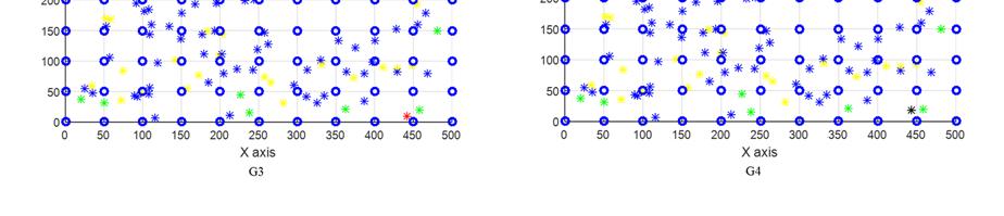
142 Figure 8.12: Local anchors for each generation (G1 to G5) using 8 anchor positions. 121

143 8.3 Edge-Based Cooperative Localization Experimental Setup 2. In this section, experiments are undertaken where a flight path attempts to localize blind nodes just around the edges of the sensing area using a mobile anchor, and then to use cooperative localization to progressively localize all the other nodes. The flight path consists of three loops at alternate 10m, 13m and 10m heights, with these loops spaced 50m apart, and the total length is 4.8km. Figure 8.13 shows the flight path and the 200 blind nodes. Table 8.5 lists the exact beacon positions. The simulation is run for 40 iterations to determine the median error for all blind nodes. A minimum of 4 anchors are required for localization. The localization error and the number of generations will be examined. Starting with 200 blind nodes, the density of blind nodes will be increased until full localization can be obtained. Figure 8.13: Localization using 50 metres spacing between beacons using 200 blind nodes and edge path planning. 122

144 Table 8.5: Position of mobile anchor node for edge path. Number Mobile anchor Number Mobile anchor Number Mobile anchor x y z x y z x y z Results for 200 Blind Nodes. Using edge path planning, many blind nodes around the edge of the area are localized by the mobile anchor (G1) and the rest of the nodes around the edges are localized in G2. However, there are insufficient local anchors (and no mobile anchors) for blind nodes in the central region to be localized. The few central nodes that are localized have very high errors. Figure 8.14 shows the localization errors for each of the nodes, and figure 8.15 shows the generations, including the large unlocalized central region. The complete table is shown in appendix F. Those nodes located in the centre of the sensing region could not be localized due to receiving less than 4 anchor positions. By comparing the localization error of square grid path and edge path using 6 anchor positions to localize 200 blind nodes, some of the blind nodes have higher error during the first generation (G1). While the nodes localized during the second generation (G2) also have higher error with the 123

145 maximum of 57 metres for node 207, 418, 0 due to weak RSSI which reached the maximum sensitivity of -90.5dB. Blind node 31 (384, 264, 0) also has high error due to the error produced by the local anchor of 430,245, 0 and 410, 307, 0 as stated in the following table. Figure 8.14: Localization error for 200 blind nodes based on generations using edge path planning. 124

146 Figure 8.15:Localized and unlocalized (UL) nodes through generation (G1-G2) for 200 blind nodes using edge path planning. 125

147 8.3.3 Results for 1000 Blind Nodes. As shown in figure 8.16, there were many blind nodes located in the centre of the sensing region that could not be localized using the edge path planning. This is because there was an insufficient density of local anchors to propagate localization into this region. Therefore, additional blind nodes are added to increase the chances of localization by local anchors. For 500 nodes, full localization was still not possible. The number of blind nodes is increased to 1000 nodes as shown in figure For this very large simulation, faster DML localization was used to reduce the very long simulation time (remembering that the whole simulation is run 40 times to get stable statistics). With this setup, all blind nodes are fully localized after the fourth generation as in figure Figure 8.16: Localization for 1000 blind nodes using edge path planning. 126

148 Figure 8.17: Localized blind nodes through generation (G1-G4) for 200 blind nodes using edge path planning. The key result in this section is not the localization error since DML was used, rather than VPML, errors are not exactly comparable, and so have not been listed. Instead, the key result for this scenario is that a node density of around 4000 nodes per square km is needed to able to do edge-based localization. On the other hand, for a 500m x 500m area, this edge-based path only reduces the total path length from 5.5km to 4.8km, which is an insignificant saving. For this scenario, a 4000 node per square km density is impractical, and edge-based localization is not recommended for this particular scenario. 8.4 Analysis. Cooperative localization, with a spacing of 50m between beacons, provides a good compromise between a short path length (5.5km) and full localization with moderate localization errors. If higher accuracy is needed then non-cooperative localization with a fine grid (10m spacing) as described in chapter 7 would be preferred. For sparse cooperative localization, a minimum number of 6 beacons gives good accuracy with a minimum number of localization generations. 127