Comparison/sensitivity analysis of various deghosting methods Abdul Hamid

Transcription

1 Master Thesis in Geosciences Comparison/sensitivity analysis of various deghosting methods By Abdul Hamid

2

3 Comparison/sensitivity analysis of various deghosting methods By ABDUL HAMID MASTER THESIS IN GEOSCIENCES Discipline: Petroleum Geology and Petroleum Geophysics Department of Geosciences Faculty of Mathematics and Natural Sciences UNIVERSITY OF OSLO [July 2011]

4

5 Contents Abdul Hamid, 2011 Tutor(s): Professor Leiv Jacob Gelius and Tilman Klüver This work is published digitally through DUO Digitale Utgivelser ved UiO It is also catalogued in BIBSYS ( All rights reserved. No part of this publication may be reproduced or transmitted, in any form or by any means, without permission.

6

7 Contents ACKNOWLEDGEMENTS... III ABSTRACT... IV INTRODUCTION... 1 ALGORITHMS TO REMOVE THE RECEIVER GHOST GENERAL DESCRIPTION (GHOST IN TIME AND SPACE) HYDROPHONE AND GEOPHONE RECEIVER GHOST CONVENTIONAL STREAMER ACQUISITION AND DEGHOSTING THE OVER-UNDER STREAMER ACQUISITION Dephase and sum algorithms Basic concept behind over-under deghosting The deghosting formula (correcting both phase and amplitude) DUAL SENSOR ACQUISITION AND PROCESSING Wavefield separation theory Wavefield separation in practice DEGHOSTING OF REAL DATA INTRODUCTION CONVENTIONAL STREAMER DEGHOSTING THE OVER-UNDER STREAMER CONFIGURATION THE DUAL-SENSOR DEGHOSTING COMPARISON ANALYSIS OF DEGHOSTED RESULTS INTRODUCTION TO METHODOLOGY AVERAGED SPECTRAL ANALYSIS THE RESIDUAL GHOST i

8 4.4 UP-SCALING OF NOISE WITH DEPTH TIME-SHIFT VARIATIONS SUMMARY AND CONCLUSIONS SUMMARY CONCLUSIONS APPENDIX A: DEGHOSTING IN TIME-DOMAIN REFERENCES ii

9 Acknowledgements My greatest thanks go to al-mighty God, the lord of the worlds, who created all the creatures and awarded the human sense to identify things in relevance. He who says: I created all creatures in pairs. If there are up-going signals then surely there should also be downgoing signals, the idea which led the scientists to find the solution to ghost arrivals in seismic data. After that, I would like to express my honest gratitude to my supervisors Leiv Jacob Gelius and Tilman Klüver for preparing this interesting topic with Petroleum Geoservices. They have been very accessible and always willing to direct me to the best way and help me to complete this project which I couldn t have done without their patience and guidance. Their great support and encouragement actually made me strong enough to complete this work. It is always pleasant to be able to get along with the people you work with, and they have been excellent. I am deeply thankful to my parents, wife, especially my brother for his economic support throughout the years...and stood by the decisions I have made and have always been there with support and guidance. Thanks to all my class-fellows, friends and faculty staff at UIO who donated their time to overcome the challenges which I ever suffered during my studies. Thanks to all the PGS staff at the marine research department for providing their guidance to complete my thesis work and also access to the seismic data volumes. This project would have not been possible without their support. iii

10 Abstract Conventional marine data is acquired by towed streamers and air-gun sources deployed at small distances below the sea level. A towed hydrophone records both upward travelling waves as well as downward travelling waves including the receiver ghost which reflects from the sea-surface and therefore changes its polarity. Every subsurface reflection is disturbed by the ghost. Ghost reflections interfere with the primary reflections and distort the frequency spectrum of the recorded seismic data. Spectral notches are introduced at different frequencies depending upon the towed streamer depth, affecting the bandwidth of the data. To minimize the ghost effect least-squares filtering can be applied. However these methods do not introduce any new information and thus do not fundamentally change the poor signal to noise ratio at these notch frequencies. So in order to suppress the effect of the receiver ghost additional data is needed. This includes acquisition using two streamers placed at different depths or alternatively using a dual-sensor streamer including particle velocity sensors. The main objective of this thesis is to investigate the performance of different deghosting techniques applied to real data acquired using conventional streamer, over/under towed streamer and dual-sensor streamer. iv

11 v

12

13 Chapter 1 Introduction Introduction In the last decades the discovery of hydrocarbons has played a vital role in the progress of nations and exploration of hydrocarbons has become more and more challenging and demanding. There is no doubt that the search for hydrocarbons is a risky business where the uncertainty level is almost at a peak. To moderate this fact modern technology and new modes of seismic data acquisition and exploration have been developed and established. The success rate for exploration and development wells has increased highly by adopting the new approaches. One of the key factors is the latest perfections in seismic data acquisition, processing and management that result into seismic images that are more sufficient to minimize the risk of drilling (Alfaro et al., 2007). The current study which represents a comparison analysis of various deghosting methods, illustrates how new performs in survey acquisition and data analysis are improving the information in marine seismic surveys. In a routine marine seismic survey a towed streamer is dragged under the sea surface by a seismic vessel. A seismic source, generally an airgun array, is towed behind the seismic vessel at some shallower depth than the seismic receivers. The seismic source generates pressure bubbles at some specific intervals. The seismic vessel sails along some predefined lines covering the subsurface targets. The pressure waves generated by the air-guns propagate into the subsurface and reflect back from the different reflectors to the seismic receivers along the streamer where they are recorded (Alfaro et al., 2007). During marine seismic data acquisition, sensors along the streamer not only record the desired wave field (upgoing signals reflected from the subsurface) but also undesired waves (downgoing reflected signals from the sea surface) called ghost. The sea surface acts as a strong reflector due to the large velocity and density contrast between water and air. The ghost has an opposite polarity as compared to the subsurface reflected signals. The recorded ghost is classified as coherent noise (Alfaro et al., 2007). In this thesis different deghosting techniques will be applied to field data acquired using both conventional streamer, dual-sensor (Geostreamer) and over/under towed streamer (Ferber, 2008). In conventional marine acquisition, source and receivers are towed at shallow depths in order to avoid notches in the seismic bandwidth (0-125 Hz). To such conventional data it is possible to apply an inverse filter to remove the receiver ghost. But this method does not 1

14 Chapter 1 Introduction add new information to the data and low frequencies are heavily contaminated with noise (Ghosh, 2000). In order to improve the bandwidth of the seismic data while doing deghosting, other types of configurations are needed. By using two streamers towed at different depths, the notches associated with the shallow streamer can be filled in using data from the deeper streamer. Alternatively, the use of a dual-sensor streamer (collocated hydrophone and velocity sensors) can be used to increase the bandwidth in connection with deghosting as both sensors show complementary notch structures (Ferber, 2008). The overall goal is to provide broadband seismic data where also the low frequencies are well preserved. These frequencies play a vital role in seismic imaging and inversion. 2

15 Chapter 2 Algorithms to remove the Receiver Ghost Algorithms to remove the Receiver Ghost 2.1 General Description (Ghost in time and space) In marine seismic surveying the air-guns and streamers are placed at predestined depths below the sea surface because of technical grounds. The water surface has an adverse effect for both air gun and receiver arrays as it distorts the source energy as well as the data recorded by the receiver. Ghosting signifies reflection of up-coming waveform at the water surface caused by the large impedance contrast between water and air (Ghosh, 2000). Thus, both source and receiver ghosts exist. The effective source signal does not only include the direct pulse but also the ghost as well. A similar kind of effect arises on the receiver side too, therefore, in marine seismic data acquisition a receiver measures the whole wavefield that is distorted due to both the source and receiver side ghosts. In traditional marine seismic exploration vessels towing arrays of airguns and streamers are used. Streamers containing pressure-sensitive hydrophones are usually towed at certain predestined depths under the surface. One of the fundamental reasons behind this is that the free surface of water is assumed to be pressure free, thus excess pressure cannot be measured here. However, from an implementation point of view, this is also done to avoid noise generated at the air-water interface due to sea waves (Aytun, 1999). In a marine seismic survey, seismic signals travel downward through the water that overlies the subsurface before being partly reflected upwards from the various interfaces representing differences in the acoustic impedance. In a calm sea, the water-air contact almost acts like a perfect reflector whose reflection coefficient is approximately equal to -1. Consequently, a hydrophone detects not only an upcoming reflection but it also records the corresponding negative reflection associated with the air-water interface (Fig.1). This ghost effect is an obstacle in seismic data acquisition and further processing is needed. This problem is obviously as old as the first marine seismic acquisition survey (Ghosh, 2000). The Ghosting is due to the reflection of up-coming P-waves from the ocean-surface which acts as a strong reflector due to the acoustic impedance contrast between water and air. This phenomenon is illustrated in Fig. 1 showing up- and down going signals. In case of a dual sensor streamer the ghost is recorded on both hydrophones and geophones. The intensity of 3

16 Chapter 2 Algorithms to remove the Receiver Ghost reflection depends upon the state of the ocean at the time of recording. A disturbed seasurface always has a lower reflection coefficient as compared to the calm sea (Gelius and Johansen, 2010). As air is less dense than water so, in common practice the reflection coefficient for the ocean-surface is assumed as 1. If u 0 t denotes the up-going recording at a receiver (R) caused by reflections from the subsurface, then the combined recording u t including the receiver ghost can be written as: u t u0 t u0t nt 1 where 2 Sea-surface d` d u t S θ D 0 R U u0 t d` < d Figure-1 A simple illustration showing the Up-and Down-going signal denoted by U and D and receiver ghost. Here θ, d and d` represent angle of emergence of the wavefront, depth of the receiver and source respectively. S denotes the source of energy from the airgun -array. In Eqs. (1) and (2) is the two-way delay time for the ghost, d is the depth of streamer (recording sensors), n is additive noise due to wind, waves, vessel etc., and c is the medium`s velocity i.e. speed of the pressure waves in water (Aytun, 1999). The approximate value of c is given as 1500 m/s. For vertically travelling waves as, the expression for delay time becomes 4

17 Chapter 2 Algorithms to remove the Receiver Ghost Hydrophone and Geophone receiver ghost As shots are fired from airgun arrays in the form of air bubbles the P-waves generated spread in all directions in the seawater and travel through the different layers in the subsurface. The reflections from different reflectors due to the acoustic contrast between different layers are recorded by sensors which are hydrophones or geophones or both. The hydrophone is a non-directional (scalar) sensor which measures changes in pressure in the medium, while in contrast to hydrophone a geophone is a directional (vector) sensor and records the particle velocity in the medium ( Gelius and Johansen, 2010). If h G represents the ghost at the hydrophone in the frequency domain, then it follows from Eq. (1) that it can be written as U U G h 1 re 1 0 e 4 (With a reflection coefficient r of -1) Here U and U represent respectively the reflected wavefield with and without 0 receiver ghost included (Fourier domain). Similarly, the ghost at the geophone will be G g 1 e 5 Because of the directional sensitivity of the geophone a sign change exists between Eqs. (4) and (5) The amplitude spectrum of respectively the hydrophone and the geophone ghost function is as (vertically travelling waves) d G h sin c 2 6 5

18 Chapter 2 Algorithms to remove the Receiver Ghost and d G g cos c 2 7 The amplitude spectra of both hydrophone and geophone are shown in the Figs.2 and 3. If h and g denote the periodic frequency notches of the hydrophone and geophone spectra respectively, then they satisfy h kc, k 0,1,2,3,... d and kc g, k 0.5,1.5,2.5,... d If the streamer is towed at shallow depth the ghost has a very short time-delay relative to the primary arrival. Instead of being recorded as a separate event the ghost appears as an unwanted complication of the wavelet including ghost notches which are undesirable nulls in the wavelet amplitude spectrum (Gelius and Johansen, 2010). G h 2 Figure 2 Amplitude spectrum of the ghost at the hydrophone side. 6

19 Chapter 2 Algorithms to remove the Receiver Ghost G g 2 Figure 3 Amplitude spectrum of the ghost at the geophone side. One choice to avoid the recording of the ghost would be deploying the streamer exactly at the sea surface with the possibility that the upward propagating signal that reflects at the airwater interface could be eliminated. Therefore there will be no ghosting in such an ideal condition. But this choice is not applicable because in this situation the streamer will be subject to a maximum amount of surface generated noise such as noise caused by waves, vessel movement, birds, winds etc. Secondly, there will be no recording of seismic data as the pressure wave requires a medium to travel through (Ghosh, 2000). 2.3 Conventional streamer acquisition and deghosting Like other acquisition methods, data acquired by a conventional streamer is ghosted due to the reflection of up-going energy from the sea-surface which acts as a strong reflector with reflection coefficient close to -1. The acquired data needs to be further processed to remove the ghost effect so that a proper image of the subsurface can be obtained (Gelius, and Johansen, 2010). 7

20 Chapter 2 Algorithms to remove the Receiver Ghost In conventional streamer data acquisition a single-sensor streamer, usually deployed with hydrophones, is towed at some shallow depth typically 8-10 meter. The hydrophone which has a non-directional property measures the pressure wavefields due to the seismic waves travelling up- and downward in the sea water. The choice of a shallow towing depth in this type of acquisition is made to avoid the notch frequencies to fall inside the seismic bandwidth (typically 0 125Hz.). As a result, the configuration enables the recording of high frequencies. For example if the cable depth is 5 meter, the first notch frequency will fall at Hz, which is outside the seismic bandwidth. But there are some other problems associated with the shallow cable depth such as: 1) The data recorded is subjected to more environmental noise caused by wind, waves and swell. 2) Loss of low-frequency signal part which is highly important for structural imaging and seismic inversion. Filtering basically means to remove or attenuate certain frequencies in order to reduce noise and improve the signal to noise ratio. Due to the destructive interference between the upgoing and down-going energy there are notches or nulls in the amplitude spectrum of the recorded data which are defined by the receiver depth and emergence angle of the seismic signal. In conventional streamer deghosting one way of removing the ghost is by designing and applying an inverse ghost filter (Yilmaz, 1987). During data processing when the inverse ghost filter is applied, the noise present at the notch frequencies scales up. Therefore a highcut filter is applied afterwards to remove this type of noise. In the amplitude spectrum the high values correspond to scaled up noise at notch frequencies because the denominator in Eq. (8) gets close to zero. The aim of the inverse ghost filter design is to obtain a filter which when convolved with the combined pulse in the time domain gives only ghost-free up-going energy (Ferber, 2008) The inverse ghost filter in the frequency domain is defined as 8 Where G (ω) is the ghost filter which is due to the reflection of upcoming wave from the sea-surface and ω is the angular frequency. 8

21 Chapter 2 Algorithms to remove the Receiver Ghost The ghost filter as given by Eq. (4) Where U( ) and U 0 ( ) are respectively, the Fourier transform of reflected wavefield with and without the receiver ghost included. 9 This implies that can be written as: 10 The amplitude spectrum of the inverse ghost filter is given by 11 Assuming vertically travelling waves and putting the value of 2d from Eq. (2) gives c 12 In general the above Equation for non-vertical travelling waves can be written as The absolute value of the wave-number vector k is given by The value of k z is given by k 2 2 z k x c So the Eq.12 becomes 9

22 Chapter 2 Algorithms to remove the Receiver Ghost The ghost due to the reflection of upcoming energy from the sea-surface is recorded both at source- and receiver side and can be removed in the same way for both cases. The depth of the streamer can be calculated by using the expression: Where c is the speed of sound in water and f 1 is the frequency at which the first notch occurs. Since the earth behaves as a low-pass filter, the higher frequencies contained within the seismic signal are relatively more suppressed than the lower frequencies after propagation through the subsurface. Hence, it is common to choose a lower value for f 1 at the receiver side than at the source side. For instance, in the case of f 1 = Hz the streamer depth d will be around 8 meters (Gelius and Johansen, 2010). In this thesis work, the filtering process is carried out in the frequency wavenumber domain. The alternative of using a time-domain least-square filter is more challenging as discussed in appendix A. 2.4 The over-under streamer acquisition In the over-under configuration two streamers are towed at two different depths positioned exactly as possible above each other and typically separated vertically by 5-10 meter. A simple appearance of over/under streamer configuration is depicted in the Fig.4. The objective of the over-under configuration is to acquire broadband data at all frequencies by combining the data recorded from shallow and deep cable. Such combination will ensure that the upward travelling wavefield contains no receiver ghosts. The key idea of using the over-under streamer configuration is to use data from the second streamer to fill in missing data at the notch frequencies of the first streamer (Posthumus, 1993). The importance of utilizing the over/under streamer is that it facilitates a larger bandwidth at both low and high ends of the recorded spectrum. Moreover, it has the potential of deploying streamers at larger depths. Hence one may operate in a quieter environment which in turn improves the signal-to-noise ratio of the recorded data. The result obtained using this 10

23 Chapter 2 Algorithms to remove the Receiver Ghost Sea-surface The over streamer The under streamer Figure: 4 Illustration showing the over and under streamers positioned at different depths and the reflection of the source signal from different layers in the subsurface. The ghost is reco rded on both streamers with different delay time (Posthumus, 1993). technique is a cable-deghosted dataset with better performance in structural imaging, inversion, and rock property descriptions in relation to other methods (Posthumus, 1993). During processing the data acquired by over-under streamers are joined together into a single dataset where the ghost has been removed. The process is generally named as deghosting. It combines the data from two streamers into a single data set in such a way that the resulting data have the characteristics of both the high-frequency of the conventional streamer data recorded at a shallow depth and the low-frequency signal of the conventional streamer data recorded at a greater depth. Hence, with the over-under technology, we can have a better time resolution, and an increased acquisition weather window. Although the fundamental concepts of the over/under combination have been known for quite some time, still the effective acquisition and processing of such data depends heavily on the capability to tow streamer pairs (one on top of the other) with a great degree of precision and accuracy (Posthumus, 1993). Different processing techniques exist for dealing with data from an overunder streamer configuration. In this thesis we have chosen to use the phase correction and adding (dephase and sum) algorithm. 11

24 Chapter 2 Algorithms to remove the Receiver Ghost Dephase and sum algorithms The theory behind the dephase and sum algorithms is that each seismic trace from both the over and under streamer is matched with a surface ghost filter in order to zero phase the ghost filter. After de-phasing and temporal alignment of the dephased data, corresponding traces from each streamer are summed to produce a single trace. Because the sum of the power spectra of the individual ghost wavelets is not flat, a further zero-phase inverse filter is applied for spectral balancing (Monk, 1990). This algorithm has the advantage that the summed traces after dephasing have an amplitude transfer function for upgoing waves that equals the sum of the power spectra of the individual surface ghosts. For this reason, the algorithm fills the notches in the amplitude spectrum in the best possible way. The drawback is that, for the de-phasing step, the method requires explicit knowledge of the surface ghost, which is usually very difficult to get (Monk, 1990). Modeling of the ghost assumes reflection coefficients based on a calm sea surface. This calm sea algorithm fails in rough sea conditions and introduces a perturbation to the output (Ferber, 2010) Basic concept behind over-under deghosting The combined effect u (t) at each of the two hydrophones corresponding to the same channel is given as a convolution of the upgoing signal u 0 (t) with a ghost filter g (t) and a additive noise term n (t). As convolution of signals in the time domain is equal to multiplication of signals in the frequency domain, then in frequency domain it can be given as: U U u l U 0 G N 15 u u u U 0 G N 16 l l l The subscripts u and l represent upper and lower streamer respectively. u U 0 and l are time-shifted versions of each other. This time shift is calculated by measuring the variations in depth of both streamers and knowledge of the medium`s acoustic velocity. While describing the ghost operators G u and U 0 G l the surface reflection coefficient is a very 12

25 Chapter 2 Algorithms to remove the Receiver Ghost important parameter (Monk, 1990). As long as the surface disturbances due to air-water interaction are small compared to the wavelength, the surface reflectivity generally is assumed to be -1. But, this is not always the case as it could only be achieved in very calm sea conditions that are rarely met in practice. However, assuming a surface reflection coefficient of -1, the ghost filters respectively for the upper and lower sensors can be described as follows: G u G l U 1 e 17 L 1 e 18 Where and represent the ghost delay time for respectively the upper and lower streamer. The ghost filter G ( ) changes both the phase and the amplitude spectrum of the received signal. The phase is given as follows: m sin ml 1 cos m tan 1 19 The amplitude spectrum of the ghost filter is given by: 20 It will vary between 0 (destructive interference) and 2 (constructive interference). Those frequencies that correspond to the ghost notches can be easily estimated from the formula f n n 21 m Here n is the notch number running from zero and upwards. This reflects that the first ghost notch occurs at zero hertz. The dephase and sum technique corrects for the phase effect of the ghost response and constructs an averaged spectrum by summation (Posthumus, 1993). This amplitude spectrum still has some information pertinent to the downgoing signal in the form of residual amplitude. A more precise result can be achieved by considering the amplitude effect of the ghost filter (Monk, 1990). 13

26 Chapter 2 Algorithms to remove the Receiver Ghost The deghosting formula (correcting both phase and amplitude) To perform deghosting, a filter should be developed such that the phase and the amplitude effect of the ghost filter can be corrected. The desired output filter gives the upgoing wavefield U 0 (ω), which is given by: F U l, U U 0 (ω) 22 Where u U0 1 e 23 U u u N u and U0 1 e 24 U l l N l When these signals are multiplied by the complex conjugate (represented by*) of the ghost filter G (ω), the phase effect is cancelled out, but the amplitude is increased due to the quadratic term, i.e. 2 u U U N 1 e U e 25 u u l L U N 1 e U e 26 l l 0 1 By adding the above two equations the following can be obtained: u U N e U N u Therefore, U 0 u 2 l u 1 e U 1 e U l 1 e u U 1 e U u 1 e 2 Or, neglecting the noise term U u l l l u l 1 e N 1 e N 1 e l 1 e 2 U u G u U l G l G 2 G 2 0 u l l u 1 e 2 u l 1 e l 14

27 Chapter 2 Algorithms to remove the Receiver Ghost Equation (28) represents the deghosting formula for over-under streamer acquisition. This implies that a weighted sum of the output from each dephased sensor can replace all missing data in the amplitude spectrum (Posthumus, 1993). 2.5 Dual sensor acquisition and processing In dual-sensor acquisition hydrophone and geophone sensors are used to measure respectively the pressure changes and the vertical particle velocities (Söllner, 2008). A combination of hydrophones and geophones placed at the same depth and lateral coordinates makes it easier to produce ghost-free data with better resolution. The dual sensor streamer can be towed at various depths without loosing low- or high frequencies, as in the case of conventional streamer data acquisition. Since the Geostreamer is routinely towed at deeper depths like between 15 and 25 m, a significant increase in operational efficiency can be obtained together with a strong reduction in sea-surface induced noise (Carlson et al., 2007). The dual-sensor acquisition is a successful method to acquire broadband seismic data. Some of the characteristics associated with dual-sensor acquisition are: 1. At both low and high ends of the spectrum, the recorded bandwidth is extended. 2. Having ability to tow at larger depths in calm conditions improves the signal-to-noise ratio. 3. The result is a cable-deghosted dataset leading to improved structural imaging, inversion, and rock property characterization (Carlson et al., 2007) Wavefield separation theory In dual-sensor processing the property used is called wavefield separation. The wavefield separation decomposes the data in upward- and downward travelling waves based on two sensors (hydrophone and velocity sensor). The velocity sensor records only the vertical component of the particle velocity so for emergence angles greater than zero the amplitude recorded by the particle velocity sensor is scaled by a factor of cos θ (Söllner, 2008, and Amundsen, 1993). To remove this effect the amplitude recorded by the particle velocity sensor is scaled by an obliquity factor i.e. 1/cos θ. As the emergence angle θ approaches 90 15

28 Chapter 2 Algorithms to remove the Receiver Ghost this scaling factor increases rapidly. For this reason a dip filter is applied to the output, typically limited to emergence angles, to avoid scaling up noise at large emergence angles. The obliquity scaling requires plane wave decomposition, and for this reason wavefield separation is performed in the f-k domain (Söllner, 2008; Aytun, 1999; Amundsen, 1993). Figure 5 Polarities of up- and down-going wave at hydrophone and geophone together with combined signal recorded by each sensor at zero - offset. The geophone whose property is to measure the particle velocity records the same polarity for up- and down-going signals while the hydrophone which is a pressure sensor records opposite polarity for up-going and down-going signals as shown in Fig.5. The reason for this different type of recording is that pressure is a scalar quantity whilst particle velocity is a vector quantity. Hence, to obtain a hydrophone measurement without the receiver ghost the upward travelling wavefield is employed (Söllner, 2008, and Amundsen, 1993). The wavefield separation method illustrated in Fig. (6) can be expressed mathematically as (vertically travelling plane waves). 16

29 Chapter 2 Algorithms to remove the Receiver Ghost These equations give the up- and down-going pressure fields. The factor of ½ is important to preserve amplitudes such that if the up- and down-going pressure fields are summed the original total pressure field (P) is recovered. Figure 6 Wavefield separation i.e. the data from the two sensors is combined to separate the wavefield into up - and down-going parts. In case the emergence angle is non-zero the amplitude recorded by the velocity sensor is reduced because only the vertical component of the particle velocity is recorded as discussed before (Söllner, 2008, and Amundsen, 1993). Hence, so the amplitude recorded by the particle velocity sensor is scaled by a factor of cos θ, i.e. V cos compared to the amplitude recorded if the velocity sensor was aligned parallel to the direction of signal propagation (as in zero offset). In order to remove these effects, the amplitude recorded by the particle velocity sensor is scaled by an obliquity factor i.e. 1/cos θ. Then the wavefield separation method becomes Z 31 17

30 Chapter 2 Algorithms to remove the Receiver Ghost The obliquity factor can be determined by multi channel recording where every single shot is recorded at a number of adjacent channels. It is necessary to determine the obliquity factor for every single event which is difficult in the time domain but easier in the f-k domain because each plane wave component maps to a particular line in f-k space. 32 Figure 7 Plane wave arriving at geophone. To determine the obliquity factor let us consider a plane wave arriving at a geophone with an emergence angle θ as shown in the Fig. (7). Consider the slowness vector S of a plane wave which can be described mathematically as Where is the unit vector in the direction of S. In terms of propagation velocity c the obliquity factor cos θ can be described as Where S z and S x are components of S in z and x-direction respectively. The above equation is valid for a 2-D wavefront. 18

31 Chapter 2 Algorithms to remove the Receiver Ghost For a 3-D wavefront in terms of the magnitude of the slowness vector the above equation becomes 33 The angular wavenumber vector K is related to the slowness vector S by the expression K = S, (34) so that the obliquity factor can be rewritten as kz ck cos z 35 K where is the vertical spatial wavenumber defined as (3D) k z kx k 36 y c or (2D) k 2 2 z k x 37 c Equations (31) and (32) can now be written as (pressure) up 1 p x x z, 2 kz down, k p, k V k, p, k p, k V, k x x 1 2 x k z z x In case of particle velocity, the decomposition equations take the form up 1 kz down 1 kz, k V, k p k, V, k V, k p, k V z x z x, 2 x z x 2 z x x 19

32 Chapter 2 Algorithms to remove the Receiver Ghost The only required parameters are the propagation velocity and density at the cable depth. These are both needed to perform the acoustic impedance correction and the propagation velocity is also required for the obliquity correction (used in the calculation of k z in Eq.37 (Amundsen, 1993). No information about ghost periods or sea surface conditions is included in these expressions, neither explicitly or implicitly. The wavefield separation relies solely on the difference between how the up- and down-going energy is recorded by the two sensors as illustrated in Fig. (6). Hence, no assumptions are needed about the properties of the water above or below the sensors, cable depths or sea surface reflection properties (Amundsen, 1993). By performing the wavefield separation in the f-k domain we implicitly assume that the cable is horizontal and the propagation velocity is constant at the cable depth. Alternative processing methods are available which allow dealing with variable cable depth (Söllner, 2008) Wavefield separation in practice Practical wavefield separation is a step by step procedure which involves the application of a number of filters in the f-k domain. The processing sequence proceeds along the following lines: Noise suppression The noise measuring characteristics of the particle velocity sensor and the pressure sensor are quite different because of their different recording behavior. Noise suppression is applied before wavefield separation. As the particle velocity sensor records only the vertical component V so at larger emergence angles its recording efficiency is not so good and z results in a poor S/N. A dip filter is applied in wavefield separation to avoid up-scaling of noise at large emergence angles. 20

33 Chapter 2 Algorithms to remove the Receiver Ghost Sensor matching In dual-sensor method deghosted data is obtained when two different types of sensors are combined together. Due to the different recording behavior of the sensors it is necessary that the recorded data are matched before they are combined. This is done by applying deterministic matching filters to the data. Low frequency conditioning The velocity sensor data is heavily contaminated by noise at the lowest frequencies. The problem is solved by reconstructing the noisy part of the velocity sensor data using the relatively clean pressure sensor data. Recorded and reconstructed velocity sensor data is typically merged between 20-30Hz. Wavefield redatuming This operation is optional. The separated wavefield (up- and down-going pressure wavefield) can be redatumed independently in order to simulate data recorded at a different depth level. This property of dual-sensor data has advantage in 4D seismic because in case of conventional streamer it is not easy to acquire the data at the same parameters. 21

34 Chapter 2 Algorithms to remove the Receiver Ghost 22

35 Chapter 2 Algorithms to remove the Receiver Ghost 23

36 Chapter 3 Deghosting of real data Deghosting of real data 3.1 Introduction The various deghosting algorithms have been presented in Chapter-2. They will now be applied to real data. Three different cases will be considered; 1. Conventional streamer deghosting. 2. Over-under streamer deghosting. 3. Dual-sensor (Geostreamer) deghosting. Prior to deghosting we have some assumptions as: (a) For conventional and Posthumus acquisitions and also partly in dual-sensor acquisition due to the low-frequency conditioning, the sea-surface is assumed to be flat during data processing. (b) The comparison of all data is being made at 8 meter depth; hence we apply wavefield extrapolation to redatum Geostreamer data (after deghosting). The seismic data employed in this study is acquired along a single sail-line having parameters as shown in Table (1). Survey name Shot no. (min. max.) Channel no. Receiver depth (m.) RDH HYD Table 1 Parameter values for surveys RDH-001 and HYD-001. RDH-001 represents data acquired using a conventional streamer, whereas HYD-001 denotes dual-sensor data acquired simultaneously in an over/under set-up. However, there was no lateral streamer steering applied to keep both cables over-under along the sailline. The data were acquired in marginal weather conditions with significant wave-heights. 24

37 Chapter 3 Deghosting of real data Figure 8 Plots showing depth variations along differe nt channels for (a) RDH-001(b) HYD-001. In case of conventional streamer deghosting, RDH-001 will be used. Over-under streamer deghosting will be carried out using RDH001 and the hydrophone part of HYD-001. Finally, dual sensor deghosting will be employed using the full data set of HYD-001. It follows from Table (1) that the actual receiver depth varies along the steamer. This is also illustrated in Fig. (8) in case of RDH-001 and HYD-001. In this thesis, the data is processed at a nominal depth (i.e. constant depth value for each receiver) to ease the processing. In case of RDH-001 it is 8m and in case of HYD-001 it is 15m. 25

38 Chapter 3 Deghosting of real data 3.2 Conventional streamer deghosting The deghosting is carried out in the frequency-wavenumber domain using a filter similar to that in Eq. (12). In order to avoid noise distortions from the notches a high-cut filter is also applied. Figure (9) gives an example of this process based on shot number 2000 from the survey RDH-001. Input data is shown in Fig. 9a. Consider the seafloor reflection inside the white box where both the primary pulse (red-blue sequence of colors) and its ghost (blue-red sequence) can be identified. The result after inverse ghost filtering is shown in Figs. 9b and c (before and after application of the high-cut filter, respectively). The pulse is now compressed in time and with the ghost part quite efficiently removed (only red-blue sequence of colors). However, the residual ghost effects are still present including the source ghost. Figure 9 shows a zoomed version of shot-point 2000, whereas Fig. 10 shows the same result for a larger part of the same shot-point gather. In this figure it is easier to see the need of the high-cut filter. Comparison between Figs. 10a and b shows that the deghosting process 26

39 Chapter 3 Deghosting of real data Figure 9 showing the seismic data in the x-t space for RDH-001, shot-2000 (a) data with ghost effect (b) after applying the inverse ghost filter (c) after applying high-cut filter. introduces noise artifacts in the data marked by the rectangle. This is due to the up-scaling of the low-amplitude parts of the original pulse spectrum. After application of a highcut filter, the data are restored as shown in Fig. 10c. 27

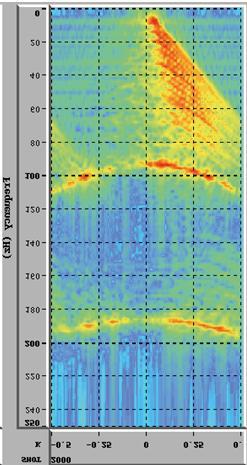
40 Chapter 3 Deghosting of real data Figure 10 Seismic data in the x-t space for RDH-001, shot-2000 (a) data with ghost effect (b) after applying the inverse ghost filter (c) after applying high-cut filter. The same observations can be made from Fig. 11 which shows how the amplitude spectrum 28

41 Chapter 3 Deghosting of real data Figure 11(a) The ghost notches in the amplitude spectrum for RDH -001 shot no (b) amplitude spectrum of the data after inverse ghost filtering (c) amplitude spectrum after high-cut filtering. changes during the same three stages. If we assume vertically travelling waves and a towing depth of 8 meter, it follows from Eq.(21) that the first and second notch will fall around 93.75Hz and 187.5Hz, respectively. The notches observed in Fig.11a do not exactly fall at 29

42 Chapter 3 Deghosting of real data these frequencies. The reason is that also non-vertically travelling waves contribute to the data representing non-zero emergence angles and larger ghost delay times. The spread of emergence angles can also be seen in the f-k spectrum shown in Fig.(13). Figure 12 Loss of amplitude level after inverse ghost filtering and application of high-cut filter (blue curve) to ghosted data for RDH-001 (green curve). Figure 12 shows plots of both ghosted and deghosted data. It can be seen that the effect of deghosting is to flatten the original spectrum on the expense of loss in the general amplitude level in the mid-frequencies. The amplitude level at low frequencies increases. Linear coherent events with the same dip will gather along a `line` in the f-k domain. In general, a wavefront can be regarded as composed of a family of plane waves with different directions (Aytun, 1999). Hence, there exist several wavenumber values for a given temporal frequency. 30

43 Chapter 3 Deghosting of real data (a) (b) (c) Figure 13 The three steps of deghosting in the f -k domain (a)data with ghost effect (b)after inverse ghost filtering (c)after additional application of highcut filter at 80-90Hz. From Fig.13a it follows that most of the energy in the original data fall within the fan defined by the two directional vectors (temporal frequencies between 20 and 80Hz.). After deghosting, noise is introduced as can be easily seen in the f-k spectrum in Fig.13b which is concentrated at the notch frequencies. The direction of waves seems to be preserved. Finally, application of the high-cut filter removes the noise artifacts in the f-k spectrum (cf. Fig.13c). 31

44 Chapter 3 Deghosting of real data 3.3 The over-under streamer configuration The over-under streamer configuration makes it possible to separate the up- and down going wavefields at the receiver using above and below towed streamers to determine the wave directions. The seismic data being used are RDH-001 and HYD-001(cf. Table 1). RDH-001 represents a conventional streamer towed at a shallow depth, whereas HYD-001 represents a dual-sensor streamer towed at a deeper depth. From the latter, only the hydrophone data are used here. It follows from Table 1 that for both datasets, the receiver depth is varying along the streamer. For both surveys, the data is processed by using the nominal depth to make the processing easier. In case of RDH-001 it is 8 meter and for HYD-001 it is 15meter. This is of course a simplification, and may lead to less optimal deghosting results. In order for the method to work well, we also need that the receivers from the two surveys are well aligned laterally. Figures 14a and b show the same shot-point with receiver ghost included for respectively survey RDH-001 and HYD-001. Use of the dephase and sum algorithm in Eq. (28) gave the result shown in Fig. 14c, where the pulse now seem more compressed (note that the source ghost will still be present). 32

45 Chapter 3 Deghosting of real data Figure 14 (a) data with ghost effect for RDH -001 at 8 meter depth (b) data with ghost effect for HYD-001 at 15 meter depth (c) deghosted data by using over-under streamer combination. More closer inspection of Fig.14 shows the effect of differing towing depth on the ghost delay time, where the combined pulse is wider in Fig.14b than in Fig.14a. The final result in Fig.14c is still affected by a residual ghost interference. 33

46 Chapter 3 Deghosting of real data Figure 15(a) Ghost notches in the amplitude spectrum of RDH -001 shot no (b) ghost notches of the amplitude spectrum for HYD -001 shot no (c) amplitude spectrum of the deghosted data from over -under streamer combination. 34

47 Chapter 3 Deghosting of real data The reason for the latter can be more easily understood if we consider the corresponding amplitude spectra as shown in Fig.(15). In case of the deeper streamer the first notch will fall at 50Hz as shown in Fig.15b. However, this notch will be compensated for by using the shallower streamer (cf. Fig.15a) to fill in the missing data. However, the second notch of the deep streamer (at 100Hz) falls almost at the same frequency as the first notch of the shallower streamer. This is due to the fact that two times the nominal depth of the shallow streamer is 2 x 8m =16m which is fairly close to the nominal depth of the deeper streamer. This implies that the spectrum of the deghosted data will contain a notch-type of region around 100Hz which makes the method very sensitivite to errors (cf. Fig.15c). (a) (b) (c) Figure 16 The three steps of deghosting in the f -k domain (a)data with ghost effect for rdh-001(b) data with ghost effect for hyd-001(c)deghosted data from combination of over-under streamers. Figure 16 shows the f-k spectrum of shotpoint 2000 for respectively RDH-001, HYD-001 and the combination. In case of the shallower hydrophone sensor, the main energy is concentrated between 20-80Hz. 35

48 Chapter 3 Deghosting of real data In case of the deeper hydrophone sensor the most energetic part falls between 10 and 50Hz. The deghosted result in Fig.16c shows that the effect of deghosting has apparently lead to more narrow energy directions. Figure 17 Amplitude spectra for over streamer (orange), under streamer (blue) and for the combined over-under streamer (green). Figure 17 represents a combined plot of the various amplitude spectra shown in Fig. (15). As already discussed, the large dip in the amplitude spectrum of the deghosted data at about 100Hz is due to the fact that both input datasets have a notch in this area. If this is the case, the dephase and sum algorithm can not restore the output data. It is possible to remove this notch by applying a high-cut filter. Alternatively, since it falls outside the seismic bandwidth the data can be used as they are. 3.4 The dual-sensor deghosting The input data used are from the HYD-001 streamer. Unlike in the previous section, both hydrophone and geophone data will be used now. As before, a nominal depth of 15m will be assumed. Fig. (18) shows a plot of shot-point 2000 for respectively hydrophone, geophone 36

49 Chapter 3 Deghosting of real data Figure 18(a) Ghost effect from hydrophone (b) ghost effect from geophone (c) deghosted data from dual-sensor combination. and dual-sensor combined data. Consider now the part of the data falling inside the white box in Fig. (18). 37

50 Chapter 3 Deghosting of real data Figure 19 Amplitude spectra of (a) ghost effect from hydrophone (b) ghost effect from geophone (c) deghosted data fr om dual-sensor combination. In case of the hydrophone data (cf. Fig.18a) one may easily see the primary pulse and its reversed polarity ghost following after. In case of the geophone data (cf. Fig.18b) the same 38

51 Chapter 3 Deghosting of real data observation can be made but now no polarity change takes place. Finally, the dual-sensor combined result in Fig.18c shows a more compressed pulse as expected. However, like in all the deghosting methods considered, the source ghost still exists. Figure 19 shows the corresponding amplitude spectra for the same shot gather. It can be easily seen from Figs.19a and b how the notches of the hydrophone and geophone sensors fall at different frequencies. In case of the hydrophone, the first and second notch fall at respectively 50Hz and 100Hz. In case of the geophone, the notches will fall in between, i.e. 25Hz and 75Hz. The deghosted data shown in Fig.19c is now characterized by a rather flat spectrum within the seismic bandwidth. (a) (b) (c) Figure 20 F-k spectra of (a) hydrophone (b)geophone (c) deghosted data. The f-k spectra for the hydrophone, geophone and deghosted data respectively, are shown in Fig.20. The following observations can be made from this figure: the hydrophone sensor shows more energy at the lower frequencies (20Hz and below) than the velocity sensor. Apparently, the velocity sensor captures slightly higher frequencies. The final deghosted 39

52 Chapter 3 Deghosting of real data result is characterized by a more uniform energy coverage over a larger frequency band with the original range of emergence angles apparently preserved 40

53 Chapter 3 Deghosting of real data 41

54 Chapter 4 Comparison analysis of deghosted results Comparison analysis of deghosted results 4.1 Introduction to methodology In this chapter I will, first of all, make comparisons between the deghosted data from all three methods using the amplitude spectrum for a selected channel (no. 13) averaging over all available shots. In the second stage I will use the time-space windows for all three types of deghosting methods to show the effect of wrong assumptions on the deghosting efficiency. Lastly, I will analyze the time shift variations between the deghosted results for a selected channel (no. 10) and all the available shots (no ) for all three types of datasets acquired by conventional, over/under and dual-sensor acquisition method. To analyze the relative time-shift variations, the datasets are processed with a procedure which is typically used for the analysis of time-lapse seismic data. The procedure analyses trace pairs which should have a similar bandwidth. Therefore, A highcut filter is applied at 80-90Hz to all the deghosted datasets. Further more, All deghosted datasets are extrapolated at a cable depth of 8meter. All the seismic displays have applied a t 2 gain which means that the signal energy is enhanced. The procedure determines a linear phase difference (i.e. relative time shift). The linear phase approximation to the phase spectrum means that the phase spectrum is represented by the equation: (f) = a + mf (38) Where (f) = is the phase at frequency f, a = phase rotation (the intercept of the line on the phase axis), m is the slope of the line and is proportional to the time shift. 42

55 Chapter 4 Comparison analysis of deghosted results 4.2 Averaged spectral analysis Figure 21 shows the averaged amplitude spectra of the deghosted data for conventional, over/under and dual-sensor streamer with increasing recording time from 300ms to 4800ms for a selected channel no.13 and averaged over all shots in the range From Fig. 21a which corresponds to the time range ms, which again corresponds to shallow depth, it can be clearly seen that the green curve representing the over/under streamer deviates from the other two curves. This means that deghosting does not work well for over/under streamer data at shallow depth. This reason is violation of the assumption, that over and under streamer are exactly positioned above each other. The violation of the assumption as mentioned above can be easily understood by the Figs. 22 and 23 which show respectively variations in the vertical- and lateral distance between over and under streamers for selected channel no. 13 and all the shots considered. There is not only the vertical depth variation, but according to Fig. 23 it can be clearly seen that over and under streamers do not lie exactly above each other. At some points they are even more than 80 meters apart. These variations lead to errors in the Posthumus method and higher frequencies are more sensitive to errors. As time-period is inversely proportional to frequency, so for a signal with larger time-period, a very small time-shift in recording due to the error as mentioned above makes a little effect. Whereas, if the signal period is short i.e. for a high frequency signal, a very small variation in the recording-time effects significantly as we see in the Fig. 21a. That is why the Posthumus (green curve) deviates from the dual-sensor (red curve) at the high frequency end in the amplitude spectrum as shown in the Fig

56 Chapter 4 Comparison analysis of deghosted results (a) Time range ms (b) Time range ms (c) Time range ms (d) Time range ms (e) Time range ms (f) Time range ms (g) Time range ms (h) Time range ms Figure 21 Channel no. 13 and shot range : averaged amplitude spectra shown by blue, green and red curves with increasing recording time ms, for conventional, over/under and dual-sensor streamer, respectively. 44

57 Chapter 4 Comparison analysis of deghosted results This difference gets smaller over the next few windows as the travel time gets larger with increasing recording time (depth). Because the timing error is small as compared to the period of the signal, we do not see the same type of deviation of green curve at low frequency end. This also indicates the stability of the low-frequency conditioning. Figure 22 Vertical distance variations between over streamer (RDH - 001) and under streamer (HYD-001) at channel No. 13 for all shots ( ). At shallow depth as shown by Fig 21 (a), the deghosting is similar for both conventional and dual-sensor data. The deghosting does not work well for over-under streamer data at shallow depth, whereas with increasing depth step by step we see that the deghosting efficiency improves and dual-sensor and Posthumus (over-under) become similar. In case of dual-sensor data at lower frequencies, we do not use measurements recorded by the geophone, instead we use data from the hydrophone. This is denoted low-frequency conditioning as mentioned earlier in the theory chapter. This explains why the amplitude spectra for the dual-sensor data and the over-under streamer data follow each other well in the low frequencies below 20Hz (cf. Fig. 21c-h). The over-under data use predominantly the deeper cable as well in the low frequencies. 45

58 Chapter 4 Comparison analysis of deghosted results From Figs.21g and h we clearly see that all curves which are flat in Fig.21a now are dipping at the higher frequencies. Generally, the amplitude of the signals decreases with time in seismic due to geometrical spreading. Furthermore, the larger recording time (depth), the less higher frequencies we have as compared to low frequencies. This is because higher frequencies get typically attenuated with increasing depth more than low frequencies. This means that the deeper amplitude spectra show more and more the influence of noise, especially at higher frequencies, as the S/N ratio decreases with depth. Figure 23 Lateral distance variations between ov er streamer (RDH- 001) and under streamer (HYD-001) at channel No. 13 for all shots ( ). In case of the conventional streamer, the data becomes more noisy at both low and high frequency ends with increasing depth. The effect of scaling up noise in the deghosting gets more prominent. The blue curve in the Figs.21 (e - h) get higher at low and high frequency ends with increasing depth. It is due to an increasing amount of noise which causes the signal to noise ratio to get worse with increasing depth for conventional streamer data. As we use inverse ghost filtering when processing conventional streamer data the noise upscaling distorts the data which can be seen in its amplitude spectrum. 46

59 Chapter 4 Comparison analysis of deghosted results (a) (b) (c) Figure 24 x-t space at ms, channel-13, for all shots ,(a)conventional streamer (b) over/under streamer (c) dual-sensor streamer. 47

60 Chapter 4 Comparison analysis of deghosted results 4.3 The residual ghost Figure 24 is a time-space view, for a selected channel (no.13) and all the available shots, of the deghosted results from all the three acquisition methods. It is a time window at smaller recording time (depth) and presents a time-range from ms. As shown by white arrows in the Fig.24b, the down-going signal which is due to the seasurface reflection is still there even after applying the Posthumus method to deghost the data. It means that the down-going ghost energy has not been completely removed and hence the ghost-free signal has not been fully recovered. It is caused by a wrong estimation of the ghost filter in the Posthumus deghosting formula (cf. Eq.28) which assumes that: (a) the over and under streamers lie exactly above each-other, (b) sea-surface is flat, (c) the depth of streamer accurately is known and (d) the reflection coefficient of the sea-surface is -1. These assumptions are not met properly. As we see in Figs. 22 and 23, both of the streamers deviate laterally and vertically, from their assumed nominal positions. This means that data is not deghosted completely and we still see residuals in the form of stripes which should have been totally removed after applying the deghosting formula as given by the Eq. (28). We do not see the same type of stripes in the conventional and dual-sensor data in Figs.24a and c because here data is completely deghosted. The low amplitude background ringing around the sea-floor reflection event, which is present in all three displays, is caused by application of the 80-90Hz. highcut filter. 48

61 Chapter 4 Comparison analysis of deghosted results (a) (b) (c) Figure 25 x-t space at ms, channel-13, for all shots , (a) conventional streamer (b) over/under streamer (c) dual-sensor streamer. 49

62 Chapter 4 Comparison analysis of deghosted results In Fig.25b we see the same residual ghost in a zoomed out version of Fig24, in the form of stripes just before the first sea-surface multiple of the sea-floor reflection event as indicated by the white arrows. Same effect, because the down-going ghost energy has not been completely removed and hence the ghost-free signal has not been fully recovered. It is because of the same reason, by applying a wrong filter. This error is the same as shown in Fig24b but just gets smaller here. If we make a comparison between Figs.24 and 25, it becomes clear that the residual ghost gets weaker with increasing recording time (depth). This is because the timing errors get relatively smaller compared to the total travel-time as deeper targets are considered. It means that Posthumus starts to work better as we move from smaller (shallow) to larger (deeper) recording time (depth). This is also seen in Fig.21, where the green curve gets closer to the red curve with increasing recording time (depth). 4.4 Up-scaling of noise with depth Figures 26 b and c show deghosted Posthumus and dual-sensor results corresponding to the time range ms, which again corresponds to deeper depth. It can be seen that both time-sections look similar and different from the time-section shown in Fig.26a, corresponding to conventional streamer deghosted data. This observation supports the results we see in the amplitude spectrum in Figs.21g-h. We see that the data shown in Fig.26a, as indicated by the white box, has higher noise levels compared to the data shown in the Figs.26b and c. In case of the conventional streamer, the reasons for this up-scaling of noise with increasing recording time (depth) are: (1) The data is acquired at 8meter depth, which is already close to the recording area where environmental noise is high. (2) During deghosting an inverse ghost filter is applied to the data which leads to an upscaling of noise. 50

63 Chapter 4 Comparison analysis of deghosted results (a) (b) (c) Figure 26 x-t space at ms, channel-13, shots , (a) conventional streamer (b) over/under streamer (c) dual-sensor streamer. 51

64 Chapter 4 Comparison analysis of deghosted results In all the three sections shown in the Fig.26 which represent deeper parts of the subsurface, we see that the noise dominates over the signal energy. It is because of the same reason as mentioned earlier that the higher frequencies get typically attenuated with increasing depth more than low frequencies. The overall signal frequency content gets smaller with increasing depth and as a result SNR gets worse. 4.5 Time-shift variations In this section I carry out a relative time-shift analysis between the deghosted data from all the three methods. Relative time-shift variations occur because of our wrong assumptions as: Sea-surface is flat. Cables are exactly over and under. Figure 27 shows the relevant time-shift variations between all the three types of deghosted data. In the Fig.27a, which shows the time-shift between conventional and dual-sensor data, we see that time-shift is highest at shallow depth and continues to decrease with increasing recording time (depth). The reason for this is as: (1) From Figs. 22 and 23 we clearly see that the hydrophone streamer at 8meter and the dual-sensor streamer at 15meter depth do not exactly lie above each other. After redatuming to 8m of dual-sensor result, both datasets are not at the same spatial coordinates as assumed. (2) The comparative effect of error decreases for larger recording time (depth) because the timing error gets smaller relative to the total travel time of the signal with increasing recording time (depth). In both for conventional and over-under streamer, the noise mainly comes from the shallow cable. At larger recording time (depth) with less SNR we see only noise comparison to noise which explains the random behavior of the time-shift estimates. The larger time-shift in the Fig.27a as compared to the time-shift in the Figs.27b and c is because in the latter two cases we compare one cable exactly the same which is common for both of the deghosting approaches and time-shift is almost zero. The reason for different 52

65 Chapter 4 Comparison analysis of deghosted results time-shift recording between 27b and 27c is because the upper and lower cables contribute differently in various parts of the bandwidth of the Posthumus deghosting result. Figure 27 time-shift variations for a selected channel (no. 10) and all the shots (no ) for (a) conventional streamer data with comparison to dual-sensor data (b) conventional streamer data with comparison to over/under streamer data (c) over/under streamer data with comparison to dual-sensor data. In all three windows in Fig.27 we see that the relative time-shift decreases with increasing recording time (depth). It is because of the same reason as mentioned earlier that the relative time-shift in comparison with the total travel time becomes smaller with increasing recording time (depth). 53