Ultrasonic Tactile Display and Field Measurement Robot

Transcription

1 Ultrasonic Tactile Display and Field Measurement Robot

2 Problem Statement for Ultrasonic Tactile Display Existing display technologies are capable of providing 2D and 3D visual feedback. These technologies stimulate only one of the user s five senses. To make the user experience more complete, the visual feedback must be accompanied by tactile feedback. Presently, the only way for visually impaired individuals to interact with a personal computers is through auditory feedback. Tactile feedback would provide an additional channel for visually impaired users to interact with information technology. Individuals suffering from deafblindness can receive intelligent information only via a tactile channel. Information technology that would benefit individuals with this condition is very primitive and yet unaffordable. Problem Statement for Field Mapping Robotic System Datasheets of speakers, ultrasonic transducers, and antennas provide limited information about the radiation profile of the device. Designers that employ constructive/destructive interference techniques require complete knowledge of the field profile of the components in order to develop proper interference algorithms. To characterize the field profile of a component or to test whether a completed system exhibits the desired interference characteristics, the designer needs to either (1) perform measurements manually, (2) send the device to a testing facility which has a characterization chamber, or (3) purchase a near-field mapping robot and perform automated measurements. Manual measurements would provide only a very rough approximation about the field characteristics. Sending the device to be characterized elsewhere is very expensive, and a single characterization may not be enough. Purchasing a field mapping robot is the best alternative, nevertheless, such robotic systems are priced at thousands of dollars and run proprietary software which. Designers needs an open-source, inexpensive, high-resolution field characterization robotic system. -1-

3 Background Research Two dimensional screens have become an indispensable part of daily experience. We are all surrounded by personal computers, televisions, and cell phones. 3D displays, although less common, are still commercially available. For decades, movie audiences could see virtual objects floating in front of them. Over the past several years, 3D TVs have become available for home users. More recently, novel 3D display technologies have been developed to render images hovering in mid-air without the aid of special glasses. Such technologies include FogScreen, Heliodisplay, Holo, Holovision, and GrImage. Some of the aforementioned technologies use a nearly invisible layer of fog to project images, which then appear to float in mid-air. Others use concave mirrors to produce a virtual 3D image of an object. The main limitation of these 3D technologies, however, is that they fool only the sense of vision. Another major drawback is that visually impaired people do not benefit in any way from such 3D technology. The next demand in 3D technology will be to provide midair 3D tactile feedback in addition to 3D visual feedback. Tactile feedback technology has applications ranging from entertainment to productivity. Movie audiences would appreciate being able to not only see but also touch the virtual 3D images floating in midair. Gamers would be even more excited about adding tactile 3D feedback in gaming. The OculusRift was invented to bring 3D visual virtual reality in gaming and it has already received over $2.5Million in backer support primarily from game enthusiast. A technology capable of complementing the 3D visual virtual reality with 3D tactile reality would be the next major demand for gaming. Another application for tactile feedback technology is to provide visually impaired individuals with an alternative channel to receive digital information. Currently, blind individuals can receive information from a personal computer only via the auditory channel. For a blind -2-

4 person, a computer screen is no different than a flat piece of glass. Tactile technology could also enable the visually impaired (as well as those without impairments) to also be able to feel what is displayed on a computer screen, thereby providing a tactile channel for receiving digital information. Today s commercial tactile technology is primitive compared to the commercial visual technology. One strategy for providing free-space tactile feedback is to attach vibrotactile stimulators or pin-array units to the user s extremities. The drawbacks of this approach is that the user always feels the presence of the tactile devices. Another strategy is to control the position of the tactile device, so that it only touches the user when tactile feedback is required. Such systems usually use a form of a robotic arm. This method also has a drawback; the tactile device is often bulky and obstructs the user s personal space. 1 One of the more recent developments in midair tactile technology is the use of airborne ultrasound to produce tactile stimulation. In the late 2000 s, a research group from the University of Tokyo built an ultrasonic tactile display prototype capable of producing tactile stimulation using low-frequency non-penetrative focused ultrasound 2. In 2013, the Interaction and Graphics research group form the University of Bristol in the UK also built an ultrasonic tactile display. The UK group, however, used an improved focusing algorithm which allowed multiple focal points to be created simultaneously. 3 Although progress has begun in exploiting ultrasound to achieve tactile stimulation, a commercial product is still not available. Only research prototypes have been constructed up to this time. 1 Non-Contact Tactile Sensation Synthesized by Ultrasonic Transducers, IEEE Noncontact Tactile Display Based on Radiation Pressure of Airborne Ultrasound, IEEE Transactions on Haptics, UltraHaptics: Multi-Point MidAir Haptic Feedback for Touch Surfaces, ACM

5 During the past several months, we have been working to replicate and extend some of the results accomplished by the aforementioned research groups. We have built a tactile display prototype with 36 ultrasonic transducers and have made significant progress toward making it capable of providing tactile stimulation. The sections that follow describe the theory behind ultrasonic tactile stimulation, the process of developing a product based on the theory, and the specifications of the current prototype. Theory of tactile stimulation via acoustic radiation pressure A detailed description of how ultrasound could be used to produce tactile stimulation, and what effects frequency and amplitude have on the perception felt by the user, can be found in a Russian research paper published by Gavrilov in Only a very brief description of the theory is provided in this report. The mechanoreceptors on the fingers and hands can perceive are most sensitive to frequencies between ~20 Hz and ~1 KHz. As frequency increases beyond 1 KHz, tactile sensitivity begins to decrease rapidly. Most readily available ultrasonic transducers operate at 40 KHz. If a test subject places his or her hand above an active 40 KHz transducer, the test subject would not feel any sensation. One of the reasons that the test subject does not feel anything is that 40 KHz is orders of magnitude above the tactile frequency range; the other reason is that a common 40 KHz transducer provides very low acoustic radiation pressure. In order of the test subject to perceive tactile stimulation, both of those challenges need to be overcome. The first problem can be solved by modulating the 40 KHz driving signal with a low frequency burst wave. The second problem can be solved using multiple transducers and driving 4 The Possibility of Generating Focal Regions of Complex Configurations in Applications to the Problems of Stimulation of Human Receptor Structures by Focused Ultrasound. L.R.Gavrilov, Akusticheskiy Zhurnal,

6 them in such a way that they all interfere constructively at a single focal point. Implementing the first solution is relatively easy, but implementing the second is much more difficult because it requires each transducer to be placed at a very precise location, it requires a circuit that is capable of driving each transducer independently at any desired phase offset, and it requires mathematical algorithm for multiple source interference to be developed. When the aforementioned conditions are satisfied, a test subject would be able to perceive tactile stimulation at the focal point at a frequency equal to the modulating frequency. Papers published by research groups from Japan and the UK indicate that the modulating frequency determines the kind of texture perceived by the test subject; both research groups used 40KHz ultrasonic transducers. The theory of tactile stimulation via acoustic sound pressure imposes no condition which requires 40 KHz frequency to be used. The paper published by Gavrilov shows that when no frequency restrictions are imposed and penetrative ultrasound is also allowed, then all of the following sensations can be achieved: tactile, temperature (warmth or even cold), tickling, itching, and various kinds of pain. However there are several reasons why 40 KHz is a very good choice for the carrier frequency. The primary reason is price and availability. 40 KHz transducers are very easy to find and are usually cheaper compared to transducers that operate at other frequencies. The second reason is that 40 KHz frequency is nonpenetrative and is inaudible. If frequencies below 20 KHz are used, there would be a very annoying audible sound. If frequencies in the MHz range are used, they would penetrate the skin and there could be health hazards associated with penetrative ultrasound. There is also a third reason why 40 KHz is a good frequency choice which has to do with physics. Low frequency sound waves have very low directionality. As frequency is increased, the aperture of the radiation code decreases. Ceteris paribus, an ultrasonic transducer -5-

7 produces a cone with aperture much narrower than that of an audio speaker. Thus 40 KHz transducers have strong directionality. MHz ultrasonic transducers are much more directional than KHz ultrasonic transducers, but that is not a desirable characteristic. In order to form a focal point one needs the radiation cone to be neither too narrow nor to wide. The cone produced by a 40 KHz transducer is right in the middle of the two extremes. Description and User Specification of Expected Final Product Our final system will be a tactile display device that is capable of producing a focal point at which tactile sensation can be felt when a user places his/her hand. The device will be capable of generating a focal point at any spatial location within some volume above the display The kind of textural sensation felt by the user will be adjustable. The focal point will be able to move in real time and thereby sweep some pattern which the user will be able to recognize. This pattern could be a triangle, a circle, a square, a sinusoidal curve or something more complicated. The main application for this device would be to transmit information to a user via the sense of touch. This transmission of information from device to user would occur over the air and be invisible to other observers since the display will have no moving components. Messages could be encoded in the patterns swept by the focal point. The user would be told in advance what message each pattern corresponds to. Additional Possible Expectations In addition to the aforementioned features, we are also planning to test whether more sophisticated capabilities can be added to the system. Prior research work indicates that different textures can be perceived when the modulation frequency of the ultrasound is changed. If we can reproduce those results and if the different textures can be detected reliably, then that would allow for another dimension of encoding of information. Moreover, we also plan to test whether rapidly -6-

8 moving the focal point would fool the mechanoreceptors to feel the presence of multiple focal points even though only one would be present at any one time. In other words, we want to test whether our system could exploit persistence of touch to yield new possibilities just like an LED systems exploit persistence of vision to achieve the illusion of dimming. This is an experiment that no research groups before us have performed with this particular technology nor even written about. Technical Specifications of Current Prototype and Expected Final Product At the beginning of the semester, we conducted a market survey to gauge interest in the device and determine what users would want out of a tactile display interface. Our survey covered both the ultrasonic transducer array and the field characterization robot, allowing us to get useful information about what design characteristics our devices should have. Table 1 shows the desired device features collected from the survey: Tactile Display Specs Desired Technical Specifications Current Progress Price $500-$1000 Cost of current prototype = $ Portability Approx. weight and size of textbook Meets weight and size requirements Daily Usage 4 hours or less per day Multi-day tests are frequently run Temperature C (or F) Device functions in these temperatures Temperature Adaptation Dynamic correction for temperature variation. No current development Table 1: Technical specifications for the Ultrasonic Tactile Display Currently, the ultrasonic tactile display prototype meets the majority of the tech specs gathered during the survey. Price, portability, daily usage, and temperature specs are all currently met at the present time. Also, a temperature adaptation feature has not been implemented. Users indicated that they d like the device to be able to dynamically adjust its focal point calculations with variations in temperature. As of right now, there has been no development of this feature. Implementation of this feature will come after progress has been made with regard to focal point optimization. -7-

9 Design of Ultrasonic Tactile Display (A) Approaches to Designing Constructive Interference: Starting from the differential wave equation, we derived the complete mathematical formalism for constructive interference from multiple point sources. The derivation takes seven pages of mathematics and is therefore omitted from this report; it is available upon request. According to the aforementioned mathematical formalism, a focal point at a position (x,y,z) can be achieved in two distinct ways: 1. The mechanical approach: All transducers are driven synchronously. In order for all of them to interfere constructively at some point (x,y,z), the transducers must be positioned at very precise location in space determined by the frequency, speed of sound, temperature, and the distance from transducer to focal point. 2. The electrical approach: Transducers can be positioned in any 2D arrangement. In order to achieve constructive interference at a point (x,y,z), each transducer must be driven at a precise phase offset relative to some reference transducer. For any given transducer, the phase offset is a function of frequency, speed of sound, temperature, and the difference: (distance from transducer to focal point) - (distance from reference transducer to focal point). Each of the aforementioned approaches has advantages and disadvantages associated with it. The primary advantage of the mechanical approach is that all transducers are driven at the same phase. This tremendously simplifies the electrical systems needed to drive the transducers. A single 40 KHz waveform generator connected to a single amplifier is all that is needed to power a system engineered using the mechanical approach. The electrical simplification provided by the first approach, however, comes with a price. Building the mechanical system would be very time consuming and expensive, because very accurate measurements need to be made before deciding where each transducer must be located. PCB would have to be ordered which allows the -8-

10 transducers to be positioned at the specific locations. A major drawback of such a system would be that if small adjustments are necessary, a completely new PCB would have to be ordered. Another drawback is that the focal point cannot be changed to a different position. There is also a third drawback. The system would produce a focal point at 40 KHz, but if the designer wants to change the frequency to 39 KHz, then the system will not produce a focal point. In fact, the mechanical approach does allow any changes to be made to a system. The electrical approach also has advantages and drawbacks. The primary advantage of the electrical approach is that transducers can be positioned anywhere on a 2D surface in any arrangement. Consequently, any cheap protoboard could be used placement of the transducers. No special PCB is needed to be ordered. However, the mechanical simplification offered by the electrical approach comes with a cost on the electrical side. The system driving the transducers is extremely complicated. The system has to be able to drive each transducer individually. For instance, for a 10 by 10 transducer array, a system with 100 outputs is needed. Moreover, the system must allow the phase offset at each output to be controlled independently. The system clock frequency must be several orders of magnitude above 40 KHz in order for fine discrete phase delays to be possible. All of the aforementioned considerations significantly increase the cost, complexity, and time required to build the electronics that power the transducers. After considering both of the foregoing approaches offered by our mathematical formalism for focal point constructive interference, we chose to use the electrical approach. Despite the complications, the electrical approach is superior to the mechanical approach because it allows changes to be made to the system without changes to the hardware when programmable logic circuit is used. It also allows the focal point to be positioned not just at one point in space but anywhere within some volume in space. -9-

11 (B) Ultrasonic Transducer Array Prototype Operation: Figure 1. Circuit diagram for a single transducer. All 36 transducers are connected in the same way. The current prototype of the ultrasonic transducer array consists of 36 transducers in a 6 x 6 configuration. Each transducer is independently driven by a TL052 operational amplifier with 0V to 20V rails. The logic behind the circuit is generated on a Spartan 3 FPGA development board and outputted through one of the three I/O banks on board. Considering each op amp is attached to its own single ended I/O pin, the phase, frequency, duty cycle, and rate of change of duty cycle of each driving signal can be adjusted independently of every other driving signal. This allows almost unlimited degrees of freedom when trying to create a focal point in mid-air. -10-

12 (C) Developing the Prototype: We have built an ultrasonic tactile display prototype that consists of a 2D array of 36 transducers. The transducers interfere constructively to produce a focal point, which we are able to position at any point in a 3D volume 15cm to 25cm above the surface of the display. Our current prototype looks as shown of Figure 2. Figure 2. Our current Ultrasonic Display Prototype Before the creation of the prototype, our initial testing took place on breadboards. After deciding that the breadboards were inadequate for larger scale testing, we began designing a replacement. We scaled up to a 6 x 6 array and used a 2200-hole protoboard to ensure identical -11-

13 distances between transducers. TL052 op-amps were selected to drive the transducers for their price, slew rate capabilities, and output current. A copper clad board was used to create a common ground for the analog and digital circuits. 26 pin ribbon cables and connectors were used to connect the Spartan Board to the op amps. Other parts were used as accessories to the main circuit and are listed in the Bill of Materials. (D) Design of Digital Control With our software running on the Spartan 3, we are able to generate 40 khz pulse trains and modulate their frequency, phase, duty cycle, and rate of change of duty cycle. Using Xilinx s ISE Design Suite, the Verilog code used to control the Spartan 3 is broken into three separate modules. Block diagrams corresponding to the Verilog code are provided in Figure 3. Figure 3. Block diagrams for (a) SystemModule, (b) DelayModule, and (c) ClockDividerModule. -12-

14 Figure 3a. MainModule -13-

15 Figure 3b. DelayModule -14-

16 Figure 3c. ClockDivideModule -15-

17 The SystemModule, allows the user to define the phase delay of each driving signal and whether or not any given output pin is on or off. These user define parameters are then funneled into the DelayModule. In this module, a counter increments itself on every clock cycle until it reaches the user defined phase delay. Once the counter is equal to the number of clock cycles given by the phase delay, a flag is set. If the user has defined this specific output pin to be turned off, the counter will always have a value of zero and will never toggle the output flag. The DelayModule calls the ClockDividerModule and passes the flag through. If the flag is set, this module begins to divide the system s 50 MHz clock down to a 40 KHz clock. This is the duty cycle can be modulated at a user defined rate. Through defining several constants within this module, the user can adjust the minimum and maximum duty cycle and the rate at which the system shifts between the two. As can be seen by the block diagram, the duty cycle modulation code requires additional logic hardware and is quite complicated. If the duty cycle remained stationary at a 50% duty cycle, this module could be replaced by a simple clock divider circuit consisting of a single counting element. The reader should bear in mind that there are 36 implementations of the DelayModule and ClockDividerModule. One of each is allocated to each driving output of the Spartan board. (E) Alternative Design Consideration for Ultrasonic Tactile Display Our current tactile display design uses TL052 operation amplifiers to drive the transducers. Before deciding to use the TL052 op amps, other possible driving circuits were considered. Among them were several other op amp models. While some of the op amps that were tested gave accurate and steady voltages, the majority of op amps could not handle the slew requirements of the system. As was expected, the cost of the higher quality op amps with faster slew rates was rather steep compared to the inadequate op amps tested. The TL052 op amps were able to drive the transducers with a relatively flat railing output and were priced much lower than many of the other op amps -16-

18 tested. After deciding to purchase the TL052 s and implement them, we have started to look for other methods of driving the circuit. The slew rate of the TL052 is within spec, but still leaves a fair amount to be desired. For the next prototype, we intend to use a bootstrapped gate driver circuit. This circuit is specifically designed for high frequency, high power, and high efficiency applications such as ours. Using a NMOS pair and a gate driver with a bootstrapping capacitor and diode, the circuit is able to send high voltage waves through an inductive load at rapid speeds. During preliminary testing, the bootstrapped gate driver excels at producing the output waveform required to drive the transducers. There rise time and fall time are much less than the current implementation. Although there are more components to this design and the system is generally more complex, the bootstrapped gate driver provides a better output waveform is more power efficient than TL052. Figure 4. Bootstapped Gate Driver Circuit. -17-

19 The driving logic behind the circuit is currently generated in Verilog code implemented in a FPGA. We could have also used a microcontroller to do the same operation. In using a microcontroller, our design would be more restricted. In a microcontroller, there are a more limited number of GPIO pins. Our Spartan 3 board has over 120 individually addressable I/O pins. When using a microcontroller, the code is executed in order from top to bottom, otherwise known as sequential execution. The only way around this general movement through the code would be the PWM function of the microcontroller that is only available on a certain number of pins. Overall, the FPGA solution is a much easier, more appropriate solution for logic generation. Another alternative design choice takes into consideration how transducers are placed next to each other. Currently our array is in a 6 x 6 square grid pattern. By positioning the transducers in this manner, large empty spaces are left at the center of every 2 x 2 subset of the grid array. To eliminate those empty spaces in the array, we could offset each row of the array by half the length of a transducer. This positioning setup would allow the transducers to be closer together, maximizing the space efficiency of the array and allowing greater sound pressure levels at a given focal point. The downside to this design is the additional complexity. Right now we have a program that calculates all of the necessary phase offsets, but if each row of the array requires a modified equation, the system can rapidly get complicated. We believe we can implement this design into our PCB fabrication without sacrificing the opportunity to test the grid array. While rearranging the array might allow us to increase the efficiency of the system and increase the sound pressure level at any given focal point, we could also create a three dimensional array. Essentially we would be creating a focal point that is equidistant to every transducer. In order to create such an array, the transducers would have to be positioned appropriately on a concave surface. If all transducers are fired at the same time, a natural focal point will form. The -18-

20 focal point can then be moved by adjusting the phase of each transducer in the same manner as our current design. We have no plans to pursue this option. Similar to the Op Amp decision, we choose to use the same Kobitone transducers that other groups have used for their designs. However, there are several types and sizes of ultrasonic transducers on the market. The other transducers on the market operate at different frequencies, have different sound pressure level profiles, and have been untested in generating focal points in mid-air. Possible ultrasound frequencies range from 25 khz to 55 khz. This range keeps the ultrasonic waves from being heard while not penetrating human skin and causing damage. We will keep using the Kobitone transducers for the foreseeable future, as there is no present need to change. Some other groups have created systems that are able to control the voltage of the pulses going to the transducers. We have also thought about creating a system like this, mainly because voltage would be an additional degree of freedom by which to control our system. Controlling the voltage with our Spartan FPGA could be done in a number of ways. Most notably, our design could incorporate a 3 state device at the output of each op amp. There are 3 state devices on the market that allow a voltage code to tell the switching element if it should pass full voltage, half voltage, or no voltage. Modulating voltage as well as every other parameter would be nice to add, but again it is an added layer of complexity that may consume too much time. The algorithm that calculates the exact amount of phase delay clock cycles only allows for a single focal point to be taken into account during calculations. If the program was able to count the phase delay clock cycles necessary for multiple focal points, the entire system would be able to make more information available to the user during operation. This new algorithm would require no new hardware, so the system wouldn t require any additional cost. By developing and -19-

21 implementing multiple focal point generation, we would be reducing the amount of energy allocated to each individual focal point. Also, the time to work on this additional project may not be worth the limited extra benefit. Design for Field Mapping Robot (A) The main frame We built the main frame of our Field Characterization Robotic System using parts obtained from three recycled flatbed scanners. Figure ## shows our robot from several different angles. The two scanners on the bottom allow motion along the X and Y axes. The vertically placed scanner supports motion along the Z axis. The scanner in the middle was connected to the scanner at the bottom using two screws. The middle scanner rides on top of the bottom scanner. To ensure that friction was minimized, two lubricated alluminum rails were attached to the edges of the bottom scanner. The middle scanner therefore rides on top of those lubricated aluminum rails. The lubricant provides very low friction and ensures a smooth ride. The vertical scanner was attached to the middle scanner using three screws. However, additional support was needed in order to keep the vertical scanner stable. Two right-angled brackets were placed to both provide the needed support and to ensure that the angle between the second scanner and the vertical scanner is exactly 90 degrees. A thin twenty centimeter long steel bar is attached to the vertical scanner. A balsa wood stick is attached to the edge of the steel bar at exactly 90 degree angle relative to the steel bar. An ultrasonic transducer, which serves as a receiver probe, is glued at the bottom end of the balsa wood stick. -20-

22 Figure 5. Pictures of the Field Characterization Robotic System -21-

23 (B) Sensors for Field Characterization Robot Figure 6. Pictures of a photointerrupter sensor and the circuit used to bias the sensor. We needed to be able to know the exact location of the probe at any one time. We used three photointerrupters such as the one shown on Figure 6. We first biased the photointerrupters by using two resistors for each photointerrupter. Figure ##b shows the circuit diagram for a biased photointerrupter. We connected the Input and Vcc ports together and we also connected the two grounds. That made the entire photointerrupter circuit assembly consists of only 3 pins as opposed to 5. After biasing the three photointerrupters, we installed them to the three scanners at the ends of the X, Y, and Z axes in such a way that when the scanning probe reaches the end of an axis, it would block the photointerrupter located at the end of that axis. This would then cause the output voltage to go high. Thus by monitoring when the output voltage goes High, we knew exactly when a photointerrupter is blocked. (C) The Control Circuit After the main frame with the stepper motors was built and after the photointerrupter sensors were added, the control circuit for the system was developed. We needed to be able to control three 12 volt stepper motors independently and we needed to be able to power up the three -22-

24 photointerrupter sensors and monitor their outputs. Thus we used an Arduino microcontroller board and three EasyDriver boards. Figure 7 shows an image of an EasyDriver board. Figure 7. (a) Pictures of the easy driver board. (b) Block diagram of connections to the EasyDriver The EasyDriver board features an H bridge which supplies power to the stepper motor connected to the board. The four pins at the top left corner is where the stepper motor is connected to. The 3 pins at the bottom provide the control for the stepper motor. When the Direction Input pin is High, the motor spins in one direction and when that pin is Low the direction is reversed. The step input is where a square wave signal needs to be applied. During each cycle of a square wave, the motor moves by one steps. Power is applied to the pins at the top right corner. There is a knob on the middle left side of the board which controls the amount of current supplied to the stepper motor. The maximum current the board can supply is 0.7mA. The board also offers microstep motion in half step, quarter step, and eighth step. The MS1 and MS2 inputs are used to set the microstepping options of the board as shown in Table 2. MS1 low high low High MS2 low low high high Resolution 1/1 Step 1/2 Step 1/4 step 1/8 step Table 2. Controls for MS1 and MS2 pins on the EasyDriver -23-

25 Each of the 3 EasyDriver boards were connected to an Arduino board and a stepper motor as shown on Figure ##. Figure 8. Connections to EasyDriver board In addition to the EasyDriver boards, we also connected the photointerrupter sensors to our Arduino board. Moreover, we also connected our data acquisition system to our Arduino and the Arduino provided the trigger pulse to the DataAcquisition system. The entire control circuit was placed in an aluminum prototype box. Holes were drilled and standoffs were mounted on the bottom and sides of the box so that all circuit boards fit in the box while enough room is left for ventilation. The pictures below show how the control system looks from inside and outside the box. -24-

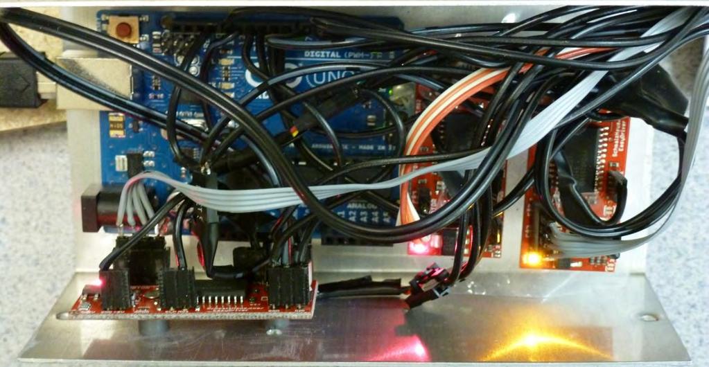
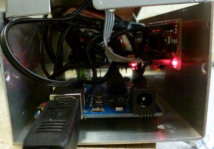
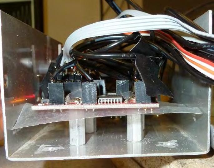
26 Figure 9. Pictures of the implemented control system. -25-

27 A block diagram of the complete data acquisition system is presented below. Figure 10. Block diagram of the complete field characterization robotic system. The block diagram above shows how the complete measurement robotic system works. Everything is controlled by the code residing on the Arduino microcontroller board. The Arduino board is connected to the three photointerrupter, to the three EasyDriver boards, and also to the NI DAQ board. The DAQ board is connected to the transducer measurement probe and to a computer. When a stepper motor makes completes a desired number of steps, the transducer measurement probes moves by that many steps. When the move operation is complete, the Arduino sends a trigger pulse to the DAQ board, which causes the DAQ board to record the data received by the probe. The Arduino waits for 5 microseconds for the data acquisition operation to complete, then it sends a move signal to the appropriate stepper motor to move to the next measurement location. -26-

28 The DAQ board is connected to a computer running LabVIEW and the data is stored in an array. After and entire measurement experiment completes, the data from the array in LabVIEW is exported to a CSV file. (D) Data Acquisition Software A National Instruments USB-6009 Data Acquisition Card was used to collect the output waveform generated by the receiver transducer. At each point of data collection, the Arduino sends a HIGH impulse to the NI DAQ to signal data acquisition. Once data collection begins, 500 points of data are collected at a sampling rate of 27 khz. (The USB-6009 DAQ has a maximum sampling rate of 48 khz, which is lower than the preferred Nyquist rate of 80 khz. The DAQ sampling rate has been reduced to 27 khz so as to optimize peak amplitude detection. The sampling frequency for optimization of peak amplitude detection has been calculated using a MATLAB program designed to sample peak values of 40 khz waveforms at sub-nyquist sampling rates.) Figure 10. Block diagram of the complete field characterization robotic system. The DataAcquisition.Vi back panel, shown in Figure ##, shows the data processing imposed on the collected points from the NI DAQ. The collected points are received as waveform data type at the output of the DAQ Assistant Vi. This data can be seen on both a Waveform Chart -27-

29 and a Waveform Graph on the Front Panel. The Waveform Chart allows the user to see the collected data in its fully expanded form after each data collection. The Waveform Graph shows each set of collected data and its relative height compared to each previous set of collected data. The waveform data is then converted into an array of type double, and the maximum value of the array is found. That maximum value is then indexed at the end of an array of maximum values of all sets of collected data. The total number of data collection cycles to be collected is calculated by the user before running the test using the formula below: # of points on X axis # of points on Y axis # of points on Z axis = Total # of Cycles The calculated value is used to define the number of iterations that the For Loop around the system goes through before completion. After the for loop has reached its designated number of iterations, the array of maximum values of all sets of collected data is converted to a comma separated values string and written to a.csv file of the user s choice. (E) Data Analysis Software In order to efficiently process and visualize the data collected by the field measurement robot, two MATLAB Graphical User Interfaces were created. Our intent in doing this was to streamline the data visualization process, and allow us to quickly shift between collected sets of data. The GUIs were made with the GUIDE tool in MATLAB, which auto-codes a template based on the GUI components. We created two interfaces: one for user input and data set selection, and one for data visualization. The two GUIs are shown below. -28-

30 Figure 11. (a) Input GUI (top), (b) Visualization GUI (bottom). -29-

31 Input GUI: After running the main code, the user is faced with the input GUI on Figure 11 a. The user then puts the following information in the respective input boxes: The name of the.csv file containing the test data to visualize. The number of X points used in the test. The number of Y points used in the test. The number of Z points used in the test. A brief description of the test. The height difference between each z plane. Upon exiting the input GUI with the user inputs in the boxes, the GUI then starts the data processing. Using the number of points in the X, Y, and Z directions, the main program reads in the.csv file defined by the user, and appropriately places the data in a 3-D array representing the tested volume. When taking the data from the.csv file and placing it into the array, the order of the data is crucial. Saved data taken by the DAQ is a 2-D array consisting of 1 row and the same number of columns as there are data points in the test. Only through a complex algorithm can the data be placed in the 3-D array that will be used for data visualization. After successfully placing the data in the 3-D array, the newly created 3-D array is saved in a new.csv file using a preset naming format including the description of the test data given by the user, and the date. Also, the array is saved in a new.csv file that requires much less data processing to use for data visualization. Determining if the array is of this format or the latter is done at the beginning of the program before any data processing occurs. Once the test data is in a 3-D array, it is ready for visualization and the Data Visualization GUI is called. -30-

32 Data Visualization GUI: Once the Data Visualization GUI is called, the user is then free to select how they re data will be graphed. Through optimization, we have reduced the number of options to just four graphing styles: Contour Color Contour 3-D Mesh Plot 3-D Surface Plot After selecting how they d like to visualize their data, the user can then scroll through each individual Z plane starting from the lowest Z plane and increasing to the highest. This version of the code allows the user to rotate, zoom in, zoom out, and see peak data with their mouse. In the future, more optimization of the code needs to be made, as the data processing algorithm needs to be perfected. (F) Driver Code After all of the aforementioned electrical and mechanical designs have been developed, the Arduino driver code that controls everything was written. The complete software driver consists of over 250 lines of optimized code, which can be divided into the following 4 sections: 1. Initialization and declaration of parameters (Figure D-1). 2. Setup section, which executes only once when the system is started (Figure D-2). 3. The main loop in which all of the scanning action is defined (Figure D-3). 4. Declaration of functions (Figure D-4 a and b). A brief description of each of the four sections is now provided. The initialization and declaration section is the most important of all four from the user s perspective. This is the section is which the USER of the robot specifies all of the parameters about the user wants the robot to do. The following parameters can be specified by the user: -31-

33 a) Offset distance along X, along Y, and along Z relative to home position. b) X, Y, and Z dimensions of the volume to be scanned. c) Resolution for X, for Y, and for Z in terms of number of data points per dimension. d) Data acquisition time for each data measurement. e) Delay Time for vibrations to die out (~0.1s for Z; ~0.3s for X and Y). Additional parameters in the initialization and declaration section are the dimensions of the display. However, this setting should only be modified if a completely new display is built, which has different dimensions. In other words, the initialization values for display dimensions should rarely have to be changed. The setup section of the code executes only when the program is started. In this section all of the utilized pins on the Arduino board are being declared as inputs or outputs. Also, there is code in this section that causes the scanning probe to return to the home position. The program makes no assumptions about the position of the probe during startup. Thus, the first physical action that takes place when the robot is started up is the probe moves toward the photointerrupters along the X,Y,and Z. Once all 3 photointerrupters become blocked, the system knows exactly where the scanning probe is located in space. The complete code that causes the probe to move to the X,Y, and Z home positions is defined in the Functions section of the code. In the setup section, the functions are simply called, which makes the code compact and easy to understand. The Setup section also contains function calls that cause the scanning probe to sweep the edges of the volume that is to be scanned. This allows the user to see whether the volume he/she specified in the initialization and declaration section is indeed the volume that will get scanned. Depending on the volume and resolution that the user has specified, a complete scan can take several days. Therefore, it is very important that the volume to be scanned is defined properly. By sweeping the -32-

34 edges of that volume before beginning the scan, the system gives a chance to the user to check whether he/she had made any errors in defining the location and dimensions of the volume. The Main Loop contains the code where all of the scanning action takes place. Most of the code contained in the main loop is simply function calls, where the actual functions are declared in section 4 of the code. In an earlier version of the driver software, we did not use functions and then the the driver code had over 500 lines of code. By defining every action as a function, we were able to reduce the amount of code by 50% and make it very easy to understand and debug. The actions that takes place in the main loop is as follows: By the time the program comes to the main loop, the probe is located at the starting position of the volume that is to be scanned. The previous section of the code ensured that this is the case. Then the probe begins moving upward along the Z dimension. It then moves forward by one increment along the X dimension and downward along the Z dimension again. Once it reaches the starting Z position, it moves one more increment forward along X. This zig-zag action between Z motion and X motion continues until the probe reaches the end of the X dimension of the volume being scanned. Then the probe moves forward by one increment along the Y axis. Then the entire X and Z action repeats but now in reverse. Once the second probe reaches the starting X position again, then a second increment forward is made along Y. This entire Z,X,Y zig-zag actions repeats until the entire volume is scanned. The last section of the code contains the function definitions. The following functions are defined in that section: 1. ReturnHome1(), ReturnHome2(), ReturnHome3() These functions cause the scanning probe to move toward the photointerrupter sensors along the x, y, and z axes, respectively. Once a photointerrupter becomes blocked, motions along the corresponding axis stops, and -33-

35 a signal is triggered that indicates that the home position along the particular axis has been reached. 2. Move1(steps), Move2(steps), Move3(steps) These functions cause the scanning probe to move by the specified number of stepper motor steps along the x, y, and z directions, respectively. 3. SweepInwardOffsetPerimeter() This is the function that when called sweeps the edges of the volume that will get scanned. This helps the user confirm that he/she has specified the proper location and dimensions of the volume that he/she wants to scan. 4. SweepDisplayPerimeter() Sweeps the area over the display. The purpose of this function is to help the user position the display exactly where the scanning robot expects the display to be located. 5. TakeMeasuremt() This is the function that when called causes a trigger pulse to be sent from the Arduino to the NI DAQ board, which prompts the DAQ board to start recording data. The measurement delay parameter that the user has specified back in the initialization part of the code resides in this function. The trigger pulse is kept high until the specified measurement delay time elapses. While this function is being executed, the scanning probe remains stationary. 6. MakeOneStep1(), MakeOneStep2(), MakeOneStep3() These are the most low level functions that only get called within the other functions. The main loop never calls these functions. They cause the x, y, and z stepper motors, respectively, to move by a single step. -34-

36 Figure 12. Section 1 of the driver code. -35-

37 Figure 13. Section 2 of the driver code. -36-

38 Figure 14. Section 3 of the driver code. -37-

39 Figure 15a. Section 4 of the driver code. -38-

40 Figure 15b. Section 4 of the driver code (continued). -39-

41 (G) Alternative Design Considerations for Field Characterization Robot Our budget limitations constrained us on the options we had for designing a field characterization system. Purchasing the hardware parts and the stepper motors needed to construct an alternative frame would have cost us several hundred dollars. Thus we decided to use recycled flatbed scanners, which already had all of the main parts we needed, and which we could obtain for free. Even then, however, we still had to make a great deal of choices as to how to build the main frame of the system. We acquired seven recycled scanners and four recycled printers and we had to finds some way of putting some of those parts together in such a way that we end up with a complete system. We considered a range of possible variations on combining the parts and we tested whether each variation would be possible with the parts we had had available. Most of the variations were not possible due to incompatibility between the parts. For instance, we considered placing a printer at the bottom and two scanners at the top as one of the variation. Another variation was to use two scanners for the X and Y motions and to provide the Z motion by moving the display itself. We even bought a board on which we planned to mount the display and have it move up and down while the scanners were moving the prove left and right. However, we decided not to go with that idea, since we found a way to mount a vertical scanner on top of the horizontal scanners that is capable of moving the probe in the z direction. After attaching the three scanners, we had to find a way of mounting the measurement probe to the third scanner. We needed the probe to be attached in such a way that reflections of the ultrasound would be kept to a minimum. This meant that the probe had to be as far from the scanners as possible, and it had to be suspended vertically on a relatively long but thin and lightweight stick. That is how we decided to attach the probe to a balsa wood stick. -40-

42 For the control circuit, we also considered a variety of possible implementations. Initially, we did not know about the existence of EasyDriver, thus we thought about designing an H-bridge ourselves that would provide sufficient current to the stepper motor drivers. However, after realizing how much time that would take to build we started looking for alternatives. We found a large variety of boards that were capable of driving a stepper motor. After looking at the specifications and the price of each boards, we ultimately decided that the EasyDriver board was the best choice for use, both because it was relatively cheap, shipped from the east coast, and it required only a very small number of Arduino pins to control the motions of the stepper motor connected to each board. The way the robot scanned the volume was also considered from several directions. Initially we thought about having the robot scan one horizontal plane at a time and return home after each horizontal plane is completed. However that was very time consuming, thus we decided to have the robot scan the volume in a zig-zag fashion. Our first driver code for robot was scanning a desired volume in a zig-sag fashion in horizontal planes. However, that was causing vibrations and requiring is to increase the amount of time allocated for vibrations to die out after each increment. Then we realized that that since the probe is suspended vertically, then we would have far fewer vibrations if most of the motion were vertical. Thus we decided to completely rewrite the main loop, so that instead of horizontal planes, it scanned the volume in terms of vertical planes. As a consequence, we also had to modify significantly the data analysis code so that it matches the format of data acquisition. -41-

43 Phase Delay Calculation Software After identifying the electrical approach as our preferred choice, we needed to be able to calculate the phase at which each transducer must be driven. Hence, we wrote a program that implements our mathematical formalism for multiple source interference. The interface of the program is shown on Figure 16. Figure 16. Phase Delay Calculation Software Interface. The program takes as an input the X,Y,Z coordinates where we want the focal point to be located, and then it calculates the phase delay at which each transducer must be driven. The phase delay is given not in terms of seconds but in terms of clock cycles of the onboard FPGA clock. Additional parameters the user must specify are the temperature of the room in Celsius (needed to calculate the speed of sound propagation), the separation distance between transducers arranged in a lattice with a square unit cell, and the frequency of the onboard FPGA clock. -42-

44 Figure 16 shows how the input and output looks for the case a focal point in the middle of the 6x6 transducer array. Two general characteristics can be observed from the data in the output table, which can be explained from intuitive considerations. The first clear characteristic is that the data in the table is symmetric with respect to the horizontal and vertical centers. The reason for this symmetry is obvious because a focal point at the center of a square array requires the four quadrants of the square array to be symmetric with each other. The second general characteristic of the data in the table is that the phase delay increases away from the transducers at the corners, with maximum phase delay occurring at the center. This can also be explained using intuitive arguments with the help of figure ##. If we want to generate a focal point at the center of a 1D array as shown on figure ##, then we must first excite the transducers farthest from the focal point and the transducer closest to the focal point must be excited last as shown on the figure. This explain the trend in the output table data that phase delay increases toward the center of the table. Figure 17. Visualization of Phase Delay. The program can calculate what the phase delays of each transducer must be in order to generate a focal point at any arbitrary X,Y,Z position. Figure 18 shows how the output table with phase delays would look if we wanted to generate a focal point somewhere between transducer B1-43-

45 and B2. We see that the maximum phase delay again occurs for those transducers closest to the focal point. Figure 18. Phase delays for focal point off center. Experimental Results Focal Point Formation Experiment (E1) For several months, we had been developing the ultrasonic tactile display according to theoretical results predicted by the mathematical formalism of focal point formation from multiple point sources. Only recently, we reached a point in the development process where we could for the first time test whether the months of work spent developing the display was worth the effort. For our first focal point formation experiment, we used 9 of the 36 transducers in a 3x3 configuration. We loaded a program onto the Spartan3 FPGA board that would drive the 9 transducers with the appropriate phase delays, such that a focal point is formed at the center of 9 at a height of 15 centimeters from the display. Figure ## shows the exact phase delays at which the 9 transducers were driven. The Phase Delay Calculation Software was used to obtain the specific phase delays for the 9 transduces, as shown in Figure 19. Figure 19. Phase delays for focal point at the center. -44-

46 In addition to the display set-up, we also had to prepare the Field Characterization Robot to scan the volume above the display at sufficiently high resolution. We wanted the robot to scan the entire volume and include the regions below and above the focal point. We set up the robot so that it would scan divide the 18 centimeters along the z axis into 21 planes. Each square plane had an area of approximately 40cm^2 and we chose to take 2500 equally spaced data points for each plane. The total number of data points that was going to be acquired during this complete test was This was the number we entered into our LabVIEW data acquisition software. After the aforementioned preparations were made for the tactile display, the field characterization robot, and the data acquisition software, we started all systems and let the experiment run. The total duration of this experiment was approximately 2.5 days. The results of this experiment were going to have a significant impact on how the project was going to proceed forward. If the experiment were a success, then it would have validated months of theoretical and experimental work, and would have shown that have made a significant progress. Conversely, if the experiment did not yield the expected results, then we may been doing things wrong during the entire time either in the theory or in the design. After nearly 3 days of anticipation the data was in, and we began analyzing it do determine whether we had succeeded or failed. For the data analysis, we used the MATLAB Data Visualization Software. Figures E1-1 to E1-21 show plots of the results from the experiment. Each of the 21 figures corresponds to a single horizontal plane containing 2500 data points. The column on the left shows a top down view of the data contained in each plane, and the column on the right shows a 3D plot of the data contained in each plane. The color represents amplitude of the received signal. Red indicates regions of maximum amplitude, yellow indicates regions of medium amplitude, and blue indicates regions of low amplitude. The color legend is shown along the side of the figure. -45-

47 Volts Figure E1-1 (a) and (b). Plane1. Figure E1-2 (a) and (b). Plane 2. Figure E1-3 (a) and (b). Plane 3. Figure E1-4 (a) and (b). Plane 4. Figure E1-5 (a) and (b). Plane 5. Figure E1-6 (a) and (b). Plane 6. Figure E1-7 (a) and (b). Plane

48 Volts Figure E1-8 (a) and (b). Plane 8. Figure E1-9 (a) and (b). Plane 9. Figure E1-10 (a) and (b). Plane 10. Figure E1-11 (a) and (b). Plane 11. Figure E1-12 (a) and (b). Plane 12. Figure E1-13 (a) and (b). Plane 13. Figure E1-14 (a) and (b). Plane

49 Volts Figure E1-15 (a) and (b). Plane 15. Figure E1-16 (a) and (b). Plane 16. Figure E1-17 (a) and (b). Plane 17. Figure E1-18 (a) and (b). Plane 18. Figure E1-19 (a) and (b). Plane 19. Figure E1-20 (a) and (b). Plane 20. Figure E1-21 (a) and (b). Plane

50 The Figure E1-1 shows the results from the plane right above the surface of the transducers. The radiation profiles of each of the 6 transducers are clearly defined. It is also clear that the transducers have some differences. We see that 3 of the transducers have amplitude greater than the remaining 6 transducers, because three of the 9 blobs have red colors corresponding to larger amplitude. Although this is not very desirable, it was to be expect that there would be some differences between otherwise identical transducers. Worth noting is the fact that the datasheets for the transducers did not specify what is the tolerance level. Thus this experiment not only allows us to test whether we are getting a focal point, but also allows us to compare how the transducers differ from one another. Figure E1-2 shows the second horizontal plane above the transducer array. We see that the amplitude s are lower compared to the amplitudes in figure E1-1. There are no red colors on the figure. We also see that the six blobs are more spread out compared to those from the previous figure. Both of the aforementioned results are to be expected since the amplitude decays exponentially with distance from the transducer, and the radiation cone coming out of a transducer becomes wider with distance from the transducer. In Figure E1-3 we begin to see interference phenomena. 16 distinct blobs are visible on the figure. A naïve viewer might assume that those 16 blobs correspond to 16 transducers. However the reason is much different. This third plane is about 2.5cm above the surface of the display, and at this height, the radiation cones of the 9 transducers begin to overlap resulting in patterns of interference. The blue regions correspond to locations of destructive interference and the yellow regions correspond to locations of constructive interference. We see that the regions of constructive interference that are in the middle have higher amplitude compared to the regions of constructive interference that are near the edges. -49-

51 In Figure E1-4 we see four distinct high amplitude peaks. These peaks are formed due to constructive interference. We also see that the remaining regions of constructive interference are also present but their amplitude is lower compared to the previous figure. Between Figure E1-4 and E1-7 we see how gradually a focal point is being formed. The constructive interference peaks seem to gradually move toward the center and ultimately produce a single point where the amplitude is maximum. As we move to planes located at higher elevation above the display, two phenomena are happening. The amplitude is decreasing because amplitude decreases with distance from a transducer, but at the same time, the focal point becomes more localized. Those two phenomena work in reverse. The first phenomenon causes a decrease in amplitude at the focal point, and the second phenomenon causes an increase in amplitude at the focal point. We see that the focal point has maximum amplitude and is also most localized in Figures E1-10, E1-11, and E1-12. As we move to planes above the 12 th plane, we observe two results. The amplitude at the focal point starts to decrease and the focal point becomes less localized. Figure E1-19 is the last figure in which we still have amplitude that falls in the red region of the legend. The last two figures have amplitude that is in the yellow regions of the legend. A very interesting phenomenon we observe in addition to those stated previously is that even as we move to higher amplitude, there is still only a single point of maximum intensity. Our mathematical formalism for focal point formation only told us what to expect at the focal point. By performing this experiment we saw a great amount of details about what is happening in the regions away from the focal point. This information could not have been obtained theoretically unless a very sophisticated mathematical formalism was developed. -50-

52 The experiment was very successful. We obtained a focal point at the center, exactly as we expected from the theoretical prediction. This experiment validated all of our previous work and confirmed that we have developed the mathematical formalism properly and that the system performs in accordance with the theory. Single Transducer Characterization Experiment (E2): After performing the focal point experiment described above, we wanted to know whether we were actually getting significantly higher amplitude at the focal point compared to the amplitude produced by a single transducer at the same height above the transducer. Thus we performed an experiment that allowed us to make a comparison between those results. We characterized a single transducer at resolution much higher than the resolution used for the focal point experiment. We set up the display so that only one transducer is active. Then we set the field characterization robot to scan the volume above that active transducer and the 8 neighboring transducers only. We divided the vertical distance into 61 planes this time, which gave us a much finer resolution along the z axis. The results of the single transducer characterization experiment are shown below. In order to save space not all 61 planes are included in the figure, but only every 3th plane. The separation between 3 planes in this experiment is approximately the same as the separation between consecutive planes in our previous experiment. This allows for a more direct comparison between the results. However, it should be noted that a one to one comparison between the results of this experiment and the results with the previous experiment is not possible because even though the separation between three planes for the single transducer experiment is approximately the same as the separation between consecutive planes for the focal point experiment, the separation is not exactly the same. Moreover, the single transducer experiment was performed at much higher planar resolution compared to the focal point -51-

53 experiment. For the single transducer experiment, each plane contained 2304 data points, but scan was only over the active transducer and its neighbor, not over the entire display as was the scan for the focal point experiment. Because of these differences in the resolution of the two experiments, a direct one to one comparison is not possible. During next semester, we plan to perform an experiment which will allow one to one comparison to be made, and the results to even be plotted on a simple two dimensional curve. But as of now, such a comparison is not possible. Notwithstanding the aforementioned complications with performing a one to one comparison, it is still possible to make a qualitative comparison between the results from the two experiments. This qualitative comparison would give a good indication for whether the results from the focal point experiment were better than the results from the single transducer experiment. In Figure E2-1, we amplitude distribution form a single transducer in the plane half a centimeter above the transducer. We see that the figure has a red region, and this turns out to be the only figure from this experiment which has red in it. As we move to higher planes, the amplitude starts to decrease. This is expected because amplitude decreases exponentially with distance from the transducer. In addition to decrease of amplitude we also see how the radiation cone spreads out as we move to higher level planes. Beyond Figure E2-8, we see nothing but blue colors. Nevertheless, up to Figure E2-14, we see that there are still special variations in the amplitude. For Figures E2-15 to E2-21, we see almost no difference; the amplitude is very low and there is no variation along the horizontal plane. A rough comparison between the two experiments clearly indicates that the amplitude at the focal point is much higher than the amplitude of a single transducer at the same height. Figure E1-13 approximately corresponds to Figure E2-13, and the difference between the two is very clear. This is another confirmation that we have been successful at achieving a focal point. -52-

54 Volts Figure E2-1 (a) and (b). Plane 1. Figure E2-2 (a) and (b). Plane 4. Figure E2-3 (a) and (b). Plane 7. Figure E2-4 (a) and (b). Plane 10. Figure E2-5 (a) and (b). Plane 13. Figure E2-6 (a) and (b). Plane 16. Figure E2-7 (a) and (b). Plane

55 Volts Figure E2-8 (a) and (b). Plane 22. Figure E2-9 (a) and (b). Plane 25. Figure E2-10 (a) and (b). Plane 28. Figure E2-11 (a) and (b). Plane 31. Figure E2-12 (a) and (b). Plane 34. Figure E2-13 (a) and (b). Plane 37. Figure E2-14 (a) and (b). Plane

56 Figure E2-15 (a) and (b). Plane 43. Figure E2-16 (a) and (b). Plane 46. Figure E2-17 (a) and (b). Plane 49. Figure E2-18 (a) and (b). Plane 52. Figure E2-19 (a) and (b). Plane 55. Figure E2-20 (a) and (b). Plane 58. Figure E2-21 (a) and (b). Plane

57 Safety Concerns Low frequency ultrasound ( KHz) has a diverse set of medical and industrial applications. Medical applications that use this frequency range include transdermal drug delivery, dentistry, eye surgery, body contouring, breaking of kidney stones, and elimination of clots. All of the aforementioned medical applications however, involve direct exposure to ultrasound where the ultrasonic probe is in direct contact with the skin or is in contact with the body via a coupling medium such as water or gel. The coupling medium an aqueous formation is what allows ultrasonic waves to penetrate the body. When low frequency ultrasonic waves penetrate the body, there is a reason for concern and a range of biological effects are possible. However, that is not of concern to our project, because our display does not use contact based ultrasound. Instead, it uses airborne ultrasound. The effects of low frequency airborne ultrasound on the human body are very different compared to the effects of low frequency contact based ultrasound. The air-tissue interface provides a highly reflective boundary, which bounces back up to 99% of the incident ultrasound energy. Consequently, airborne exposure has only limited penetration into the human body. Therefore, the impact of airborne ultrasound on the human body is mainly confined to external body organs such as the skin, the ears, and the eyes. For very high sound pressure levels, above 190dB, airborne ultrasound will lead to cavitation in the human body. For lower sound pressure levels, heating effects are the only concern. For sound pressure levels above 155dB, the temperature on the human body can be raised rapidly to damaging levels. Between dB only slight heating of the skin occurs 5. The transducers we are using have SPL of 120dB at a height of 30cm. Doubling the number of transducers and focusing the ultrasound generally increases the SPL by about 3dB. With this 5 Bio-Effects and safety of low intensity, low frequency ultrasonic exposure, Ian V. McLoughlin, Sunita Chaugan, Farzaneh Ahmadi, Gail ter-haar. Nanyang Technological University. -56-

58 information we can construct the following table that compares number of transducers to max SPL possible. Transducers SPL 1 120dB 2 123dB 4 126dB 8 129dB dB dB dB dB dB dB dB dB dB Figure 20. Comparison between number of transducers and total Decibel output From the table above, we see that to reach SPL of 155dB, where temperature damage becomes possible, it would take over 4000 transducers. Therefore, for our current prototype which has only 36 transducers, there are not health hazards. Moreover, even our next prototype, which we indent to have 100 transducers would produce SPL of less that 140dB at the focal point, thus there is again no health hazard associated with that exposure of airborne ultrasound. Ethical Considerations The ultrasonic tactile display and the field measurement robot are not ethically immoral products. Quite the contrary, most human computer interfaces discriminate against people who are disabled. Anyone who cannot see, or hear, or both, is virtually unable to use a modern computer. Braille readers and other such devices are available, but are crude and extremely expensive. Our product aims to fix this problem. By enabling disabled people to interact with computers in a more complete manner, the ultrasonic tactile display will improve the lives of people who use it. Since the field measurement robot is used to aid people through the research and development phase of -57-

59 product design, there s not any moral conflict when using it. The only way either device could be considered immoral, would be if either device was used for the explicit purpose of hurting someone. If someone were to throw either the ultrasonic tactile display or the measurement robot at someone else, then the person whose actions caused the device to inflict pain is immoral. In that case, calling either device immoral would be a large stretch. The voltage, (maximum of 20V), and the current, (maximum of 120mA), is low enough to only inflict limited damage to humans. We will take precautions to ensure that the products are robust and strain relief is used to reduce wire fraying. Our final design will be encapsulated in a 3D printed shell, guarding users from any sharp edges and electrically live components. Governmental Regulations FCC Title 47, Chapter 1, Subchapter A, Part 18, Subpart A Section within this regulation dictates The rules in this part, in accordance with the applicable treaties and agreements to which the United States is a party, are promulgated pursuant to section 302 of the Communications Act of 1934, as amended, vesting the Federal Communications Commission with authority to regulate industrial, scientific, and medical equipment (ISM) that emits electromagnetic energy on frequencies within the radio frequency spectrum in order to prevent harmful interference to authorized radio communication services. This part sets forth the conditions under which the equipment in question may be operated, (FCC Title 47, ) 6. This generally says that the EMI radiation of any industrial, scientific, or medical equipment must be reduced to within a limit in order to prevent interference with regulated frequency bands. Considering both of our devices are scientific and that ultrasound is used in 6 FCC. "ECFR Code of Federal Regulations." ECFR Code of Federal Regulations. FCC, 4 Dec Web. 07 Dec

60 medical applications, we can use the specifications dictated in as guidelines for designing to reduce EMI radiating from our device. Using the specifications in , ultrasonic devices radiate less than 400 watts of energy, meet a Field Strength Limit of 2,400 µv/m of energy per khz at a range of 300 meters. At the same time, our device must follow strict radiation levels at frequencies from MHz. Our device must meet the EMI restrictions of the table below: Frequency(MHz) Field strength limit at 30 meters (µv/m) When designing our devices, there are a variety of ways to limit EMI radiation. Our focus will be the elimination of unintended radiators. These usually arise from highly repetitive signals with high harmonic content, such as clocks. Power lines can also conduct and radiate EMI. Since our device can be operated in an industrial and commercial setting, we must follow the requirements of a Class A/B device. In our design, we will need to treat all cables as antennas, as these are the largest physical dimension signal carrier in the system. Assumptions cannot be made about the shielding capabilities of wires unless tested. We can also reduce the overall EMI radiation of the PCB by using multiple layers. By using a multilayer PCB, power distribution capacitance lowers at high frequencies because of the distributed capacitance of the power and ground planes. Also, high frequency ground bounce can be reduced in PCB s by reducing the overall ground impedance through a ground plane. Figure 21. EMI Power Restrictions at given Frequencies, (Source: FCC Website) -59-

61 RoHS Compliance RoHS, or Restrictions of Hazardous Substances, restricts the use of specific hazardous substances in electronic devices. Also called Directive 2002/95/EC, RoHS restricts the use of lead, mercury, cadmium, hexavalent chromium, polybrominated biphenyls, and polybrominated diphenyl ethers. These substances have a history of being harmful to landfills and the environment in general. WEEE, or Waste from Electrical and Electronic Equipment, is also used to provide consumers with avenues to recycle and dispose of old electronics. Any device that does not meet these specifications cannot be sold in the European Union. In order to design our devices to be RoHS compliant, we will not be using any of the aforementioned substances in our design. While we will actively recommend proper recycling of our device to certified electronic waste services, there we cannot control consumer s actions with regards to the disposal of our device. 7 Patents Although we acknowledge that other groups have completed projects similar to these devices, a patent search is necessary to uncover what claims have been made with the technology we are using. Regardless of what has already been patented, the process is uniquely educational, as every person applying for a patent must reveal the intricacies of their invention. We have compiled two patents relating to tactile sensations with ultrasonic vibration technology. These patents apply to tactile interactions between humans and surfaces, as our project deals exclusively with airborne tactile sensations, but the connection between the two is apparent. In these patents, the inventors and their corresponding organizations detail their ideas and how they could be implemented in a real world application. 7 European Union. "Recast of the RoHS Directive." - Environment. European Union, 30 Oct Web. 07 Dec

62 Touch Sensitive Display with Ultrasonic Vibratio ns for Tactile Feedback Patented in 2008, this patent is comprised of a mobile communication device that has the ability to provide users with haptic feedback based on input to the mobile device. Summary of claims: The inventor claims that a keypad assembly containing a touch sensitive cover, an ultrasonic element and a display can provide users with a tactile interaction with a user. This mobile device s display is contains a liquid and an ultrasonic element. The ultrasonic element sends ultrasonic waves to produce the haptic feedback to the user. The logic of the display will allow the device to pin point the user s fingers and activate the ultrasonic element corresponding to that position. The display also allows for input from a touch sensitive surface. On each touch of the surface, ultrasonic elements will vibrate and allow tactile feedback from under the surface. Input will be sensed with a capacitive film. The display also has the capability of showing a character at the point of contact. Several keys are possible on the device using a liquid crystal display. Since the keys require input ability, they will also have a capacitive film. The ultrasonic element will be made of piezo-electric material. That means that the display will contain piezo-electric ultrasonic elements. The display s touch sensitive surface will use glass at the point of interaction with the user. The bottom of the enclosure is in contact with the touch sensitive surface. The invention allows the user to feel a tactile response at any given location on the surface of the mobile device. Upon touching the device, a capacitive touch sensitive layer will give the position of the touch interaction to a logic circuit. This logic circuit will determine what the location on the screen has been touched. From this location, the logic circuit will then have to return the user s selected action from the processor to the screen. In addition to that, the logic circuit will also have to activate certain piezo-electric ultrasonic elements under the surface of the screen. These piezo-electric elements vibrate at ultrasonic frequencies and transmit these -61-

63 frequencies through a liquid underneath the screen. The logic circuit has to select which piezoelectric elements to turn on and which to leave off, or else the entire screen would vibrate. This method of generating selective ultrasonic vibrations allows the user to only feel a tactile response from the device at specified locations. If the user is trying to type on a plurality of keys displayed by the liquid crystal display, the tactile feedback from the ultrasonic elements and the logic circuit would only be activated on the location of the keys that were pressed. In the figures below, one can see the flow chart of logic, stemming from the control logic. 8 Figure 22. Figures from the patent Tactile Stimulation Device and Apparatus Summary of Claims: The tactile stimulation device is comprised of a plurality of linear ultrasonic actuators. These actuators are aligned in the vertical direction to a contact surface with which a user would interact. There is also a plurality of contact portions that are formed with the movers of the linear ultrasonic actuators. The linear ultrasonic actuators themselves are driven with electrical signals of the ultrasonic frequency that the actuators are supposed to oscillate at. They also have a moving axis in an up and down direction. The tactile stimulation of the device is caused 8 Helena Elsabet Pettersson, Sony Ericsson Mobil, US Patent: WO A2-62-

64 by the action of the linear ultrasonic actuators on the plurality of contact portions on the surface of the device. The linear actuators are disk-shaped with a bimorph type that is concavely and convexly changed in shape according to the electrical moving signal. The ultrasonic transducers are disposed alternately in different heights and at varying lengths of the moving axes from the adjacent ultrasonic transducers. This alternately moving of adjacent ultrasonic transducers allows for a longer maximum displacement between two transducers or moving axes that move with accordance to the driving electrical signal than from a single transducer alone. The tactile sensation device is comprised of an image acquisition unit for taking a picture of the object that is to be reproduced with the device. This image processing unit takes the picture and filters it into signals that can be processed. The device then takes these signals and sends appropriate electrical signals to the linear ultrasonic transducers in order to replicate the feel of the object. Specified tactile sensations will be transferred to the user via touch based on the image/ signals generated from the image processing unit. The linear actuators can generate different sensations and tactile feedback based on the frequency sent through the electrical driving signals. This device allows for the miniaturization of haptic feedback devices and allows for replication of sensations that would not otherwise have been possible. This device can be used in braile readers, PDA s, and an assortment of mobile devices. By allowing users to have a greater spectrum of interaction with their devices, there is a new level to the information transfer between the device and the user. Below are figures from the patent that illustrate its use: 9 9 Ki-uk Kyung, Jun-Seok Park, Dong-Won Han, US Patent: US A1-63-

65 Figure 23. Figures from the patent Project Management At the beginning of the project, we had predicted that the completion of the PCB and the majority of the focal point optimization would be done by the end of the Fall semester. Unfortunately, our project is a little behind schedule due to setbacks attributed to time management with full course loads. Below is the initially proposed project development time line with the corresponding sequential task list: -64-

66 Figure 23. Original Gantt chart from beginning of the semester. Figure 24. Original PCB Fabrication Gantt chart. -65-

67 Figure 25. List of tasks from beginning of the semester. Figure 26. List of tasks from beginning of the semester for PCB Fabrication. -66-

68 Our original project schedule was overly optimistic with regard to the completion of the PCB fabrication and testing of all subsets of the prototype array. The majority of our time in lab was spent debugging the array and its software, as well as testing subset arrays up to a 3 x 3 grouping of transducers. While we were not able to complete the PCB design and fabrication, we have compiled a growing list of features to be implemented on the PCB. Below is the realized Gantt chart and corresponding task list of our fall semester progress: Figure 27. (a)final Gantt chart from the end of the semester. (b) List of tasks for (a) -67-

69 As can be seen in the Gantt chart above, the majority of our time was spent trying to debug the system and get reliable operation. Focal point formation took about the same amount of time as expected. However, running tests took multiple days and locked up almost all of the resources available in the lab. If we weren t testing, we were debugging. The opposite also applied. After our first initial testing, we determined that the field measurement system was prone to vibration issues at the receiving transducer. In order to avoid this vibration at the output, a reworking of the code was required. This took approximately a week to perfect and was an unexpected addition to the task list. Another setback came from the visualization software. After the field measurement robot code was altered to better tackle vibration issues, the visualization software had to be changed in order to account for a different order of input data. Optimization of the visualization code was unexpected and took longer than expected. Looking forward, the tasks that were not completed during the Fall semester will be added to the work load of the Spring semester. A preliminary analysis of next semester has been completed and is shown in the Gantt chart below: -68-

70 Figure 28. (a)proposed Gantt chart for next semester. (b) List of tasks for proposed Gantt chart. -69-

71 Bill of Materials Part Description Supplier Supplier P/N Manufacturer Manufacturer P/N Website Price Per Unit Quantity Total Price Easydriver Motor Control Board SparkFun CC BY-NC-SA 3.0 Brian Schmalz CC BY-NC-SA $ $ Arduino Uno Amazon A Arduino B006H06TVG $ $ Recycled Scanner Motors N/A N/A N/A N/A N/A $ - 3 $ - Recycled Photo Interrupter Sensors N/A N/A N/A N/A N/A $ - 3 $ - Ultrasonic Transducer, (Used for Reception) Mouser ST16-ROX Kobitone ST16-ROX $ $ 4.48 Recycled Aluminum Rails N/A N/A N/A N/A N/A $ - 2 $ - Recycled Cables, Connectors, and Power Cord N/A N/A N/A N/A N/A $ - 6 $ - LabVIEW USB-6009 DAQ Ted NI $ $ Screws Fastenall N/A N/A N/A N/A $ $ 4.00 Balsa Wood Stick Hobbytown USA N/A N/A N/A N/A $ $ 0.10 Right Angle Shelf Brackets Lowes N/A N/A N/A N/A $ $ 8.36 Super Glue Hobbytown USA N/A N/A N/A N/A $ $ 1.00 Subtotal: $ ECE Resources $ (299.00) Total: $ Part Description Supplier Supplier P/N Manufacturer Manufacturer P/N Website Price Per UnitQuantity Total Price Bill of Materials Spartan 3 Starter Kit Ted (obsolete) N/A Xilinx N/A N/A $ $ Ultrasonic Transducers Mouser ST16-ROX Kobitone ST16-ROX $ $ Protoboard with 2200 Holes RadioShack Radioshack $ $ 7.98 TL052 Op Amps Digikey TL051CP TI ND $ $ Approx. 6" of 26 Position Ribbon Cable N/A N/A N/A N/A N/A $ $ Position Ribbon Cable Interconnect Amazon B007R2JEMY PC Accessories 28-26Pin-SOCKET-5PKhttp:// $ $ 1.80 Copper-Clad PC Board RadioShack Radioshack $ $ 4.49 Terminal Connector Digikey ND TE Connectivity $ $ Lead Free Solder RadioShack N/A N/A $ $ 8.49 Benchtop Power Supply N/A N/A N/A N/A N/A $ $ Heatshrink N/A N/A N/A N/A N/A $ $ 2.50 Cables N/A N/A N/A N/A N/A $ $ 2.00 Header Pins Ted N/A N/A N/A N/A $ $ 0.20 Subtotal: $ ECE Resources: $ (276.70) Figure 29. BOM For Ultrasonic Display. Figure 30. BOM For Field Characterization Robot. -70-

72 As can be seen from the BOM, the current cost to construct our device is $ We were able to cut most of our costs by sourcing parts and equipment from the Senior Design Lab and our office in the Lehigh Display Lab. Our price of construction was only $214.53, only because we were able to take advantage of the resources available to us. The main costs required to build our prototype stems from the price of the Spartan 3 board and the transducers at $199 and $160.20, respectively. If this device were to be sold to consumers in the condition that it is in, additional savings would be possible by building an inventory of bulk priced items, such as: transducers, op amps, ribbon cable, etc. Future Plans After we return from break, we plan to run an experiment where we make a direct 1 to 1 comparison between one transducer and focal point. We want to plot amplitude vs. distance for both cases on the same graph. Then we will augment the graph by testing not only 3x3 configuration but also 4x4, 5x5, and 6x6. All of the results will be plotted on the same graph. Generating this graph will not take more than 2 days, because for this experiment we will only scan a single column exactly where the focal point is located one column for each of the specified configurations. This will allow us to see how much does each consecutive square of transducers contribute to the amplitude. Another experiment we want to run is to test whether we can produce a focal point off center. We already have the program that calculates what the phase offsets have to be for a focal point at any desired location. Thus to perform this test, we would simply have to input the delay values obtained from the program into the Spartan3 FPGA board and run a measurement. The measurement would take two to three days to complete. The first off-center focal point experiment will be performed with only 9 transducer in a 3x3 configuration. Once we validate that the results -71-

73 are successful, we will move forward and perform off-center focal point experiments with more than 9 transducers. Then, the results from the various focal point experiments will be compared to quantify by how much the amplitude of the focal point decreases as the focal point is shifted away from the center of the display. Depending on the results of the aforementioned experiments, we may have to make offset corrections to the focal point generation algorithm, so that a more localized focal point is achieved. We might also consider the possibility of creating a more sophisticated algorithm for focal point formation, which will allow us to have a more localized focal point. This alternative algorithm would use only some of the transducers for creating a focal point. The remaining transducer would be used to create regions of destructive interference around the focal point. Besides the experiments related to focal point formation and optimization, we will also have to perform experiments where we include modulation to the ultrasound. A major milestone will be completed when for the first time we become able to receive tactile sensation at the location of the focal point. After this milestone is complete, we will test whether we can create different textures that the user can perceive. An alternative layout of the transducers is one possibility we are considering. In our current prototype, the transducers are arranged in a square fashion. This leaves some space between the transducers. For the final PCB, we might choose to rearrange the transducers in a honeycomb pattern, so that they are more compact. After coming back from break, one of our first tasks will be PCB fabrication. The PCB will allow for a 10 x 10 array of transducers that are individually driven by a new gate driver circuit that was discussed in the alternative designs section of this report. The advantage of switching to this circuit is derived from the exceptional output waveform and incredibly fast slew rate. -72-

74 Considering the gate driver circuit is specifically designed for applications that are driving high voltages at high frequencies, our hope is to create a more perfect sinusoidal waveform out of the transducer. This circuit will come with additional complexity and components, but the cost will be roughly the same as the TL052 implementation. Having already tested the gate driver circuit whilst driving transducers, we can say with confidence that the system will be improved. The Pspice schematic of the gate driver circuit and some output waveforms of the gate driver circuit are provided below: Figure 31. Pspice Model of the Gate Driver Circuit Figure 32. Simulated output vs. Experimental output -73-