LOSSLESS IMAGE COMPRESSION EXPLOITING PHOTOGRAPHIC IMAGE CHARACTERISTICS

Transcription

1 LOSSLESS IMAGE COMPRESSION EXPLOITING PHOTOGRAPHIC IMAGE CHARACTERISTICS A THESIS SUBMITTED TO THE UNIVERSITY OF MANCHESTER FOR THE DEGREE OF MASTER OF PHILOSOPHY IN THE FACULTY OF ENGINEERING AND NATURAL SCIENCES 2008 Issa Abbasi School of Computer Science

2 Contents Contents...2 List of Tables...5 List of Figures...6 Abstract...7 Declaration...8 Copyright...9 Acknowledgements Introduction Data Compression Redundancy Methods of Compression Equal length and Unequal length codes Statistical Compression Image Basics Digital Image Image Resolution Image Sampling Grey-Levels Quantization Neighbours of a Pixel Raster Scan Types of Images Summary Research Aims Contributions Background Image Compression Compression Process Lossy Compression Methods

3 2.1.3 Lossless Compression Methods: Differential Pulse Code Modulation Importance of DPCM The MED predictor Design of Predictors Proximity map Inferences Using more neighbours as predictors: Union of top and left predictor Nature of pixels along different axes Observation Predictor based on Least Differences Method Definitions Result Experiment: Effect of difference on pixel value Difference Weighted Average (DWA) Predictor Comparison Experiment Performance of Predictors Image Segmentation Edge detection Detection and Segmentation in Rough and Smooth regions Hypothesis Hybrid threshold predictor Results Composite predictor Method Results 56 3

4 4. Results and Analysis Performance of DWA predictor Computaitional Cost of DWA method Analysis of Hybrid Threshold Method Average Frequency Graphs Selection of Threshold Gain Analysis of Combined Method Comparison of Composite method with Threshold Method Conclusion Summary Discussion Future Directions Identified features for further exploitation Progressive computation of weights...73 Appendix A...74 Bibliography

5 List of Tables TABLE 1 PROBABILITIES OF SYMBOLS TABLE 2 ASSIGNMENT OF CODES BY HUFFMAN CODER TABLE 3 THREE ROWS AND THREE COLUMNS DATA OF PICTURE OF THE GIRL TABLE 4 PIXEL DATA FROM THE PICTURE OF GIRL TABLE 5 HIT BY FOLLOWING LOWER OR HIGHER DIFFERENCE TABLE 6 COMPARATIVE GAINS OF MED AND DWA TABLE 7 MED AND DWA ALGORITHMS TABLE 8 PIXELS CONTAINED UPTO EACH EDGE INTENSITY LEVEL

6 List of Figures FIGURE 1-1 HUFFMAN CODING FIGURE 1-2 MONOCHROME DIGITAL IMAGE FIGURE 1-3 NEIGHBOURS OF A PIXEL FIGURE 1-4 RASTER SCAN ORDER FIGURE 1-5 CONTINUOUS-TONE IMAGE FIGURE 2-1 IMAGE AND HISTOGRAM OF GREY-LEVELS FIGURE 2-2 DIFFERENCE IMAGE AND HISTOGRAM OF DIFFERENCE VALUE FIGURE 2-3 NEIGHBOUR CONVENTIONS FIGURE 3-1 PICTURE OF GIRL AND PROXIMITY MAP FIGURE 3-2 PICTURE OF HOUSE AND PROXIMITY MAP FIGURE 3-3 PICTURE OF TREE AND PROXIMITY MAP FIGURE 3-4 DIFFERENCE IMAGES FIGURE 3-5 HITS USING TOP AND LEFT PREDICTORS FIGURE 3-6 SMOOTH PORTION OF THE PICTURE OF GIRL FIGURE 3-7 GRAPHS OF 3 ROWS AND 3 COLUMNS OF PICTURE OF GIRL FIGURE 3-8 HORIZONTAL AND VERTICAL DIFFERENCES FIGURE 3-9 ROW AND COLUMN PIXEL VALUES PLOTTED ON THE SAME AXIS FIGURE 3-10 NUMBER OF HITS AND ENTROPIES USING DIFFERENT PREDICTORS FIGURE 3-11 PERFORMANCE OF DIFFERENCE WEIGHTED AVERAGE PREDICTOR FIGURE 3-12 COMPARISON WITH MED PREDICTOR FIGURE 3-13 PIXEL WISE COMPARISON BETWEEN MED AND DWA FIGURE 3-14 PIXELS USED TO DETECT EDGES FIGURE 3-15 ORDER OF PREDICTION OF PIXELS IN AN IMAGE FIGURE 3-16 PERFORMANCE OF DWA AND MED FOR AN IMAGE OF TREE FIGURE 3-17 COMPARISON OF MED, DWA AND HYBRID THRESHOLD PREDICTORS FIGURE 3-18 COMPARISON OF MED, DWA, HYBRID THRESHOLD AND COMPOSITE PREDICTORS FIGURE 4-1 PERCENTAGE GAIN IN ENTROPY USING DWA PREDICTOR AS COMPARED TO MED PREDICTOR FIGURE 4-2 AVERAGE PERFORMANCE OF DWA AND MED FIGURE 4-3 COMPARATIVE FREQUENCIES OF HITS OF DWA AND MED FIGURE 4-4 PERCENTAGE GAIN IN ENTROPY USING HYBRID THRESHOLD PREDICTOR AS COMPARED TO MED FIGURE 4-5 COMPARISON BETWEEN PERFORMANCE GAINS OF THRESHOLD AND COMPOSITE PREDICTOR WITH MED PREDICTOR FIGURE 4-6 PERCENTAGE OF TOTAL PIXELS SCANNED UP TO THE EDGE INTENSITY LEVEL FIGURE 5-1 PIXEL WISE COMPARISON BETWEEN MED AND DWA

7 Abstract Digital Images require large storage space as higher and higher resolution becomes possible, at the same time as the storage becomes cheaper it becomes feasible to store rather than discard useful detail. Compressing digital images not only saves storage space but reduces transmission time if the image has to be transmitted. Depending on requirement images are either compressed using lossy or lossless compression methods. Lossy methods allow very large compression ratios as compared with lossless compression methods at the expense of losing information. In cases where smallest image detail matters such as in medical image processing, preservation of art work and historical documents, satellite images and images from deep space probes images are compressed using lossless image compression methods. Despite the importance of lossless image compression of continuous-tone images there is a paucity of standard algorithms. This thesis analyses different methods of lossless image compression which use prediction based on context. These methods exploit information from context and the performance of these methods is proportional to the precision of prediction. There may be more room for compression because more information can be exploited from the context. It is demonstrated that combining existing methods or including more information from the context can improve prediction results thereby improving compression ratios. Results are compared with JPEG-LS which is state of the art method in Lossless Image Compression. 7

8 Declaration No portion of the work referred to in the thesis has been submitted in support of an application for another degree or qualification of this or any other university or other institute of learning 8

9 Copyright The author of this thesis (including any appendices and/or schedules to this thesis) owns any copyright in it (the Copyright ) and s/he has given The University of Manchester the right to use such Copyright for any administrative, promotional, educational and/or teaching purposes. Copies of this thesis, either in full or in extracts, may be made only in accordance with the regulations of the John Rylands University Library of Manchester. Details of these regulations may be obtained from the Librarian. This page must form part of any such copies made. The ownership of any patents, designs, trade marks and any and all other intellectual property rights except for the Copyright (the Intellectual Property Rights ) and any reproductions of copyright works, for example graphs and tables ( Reproductions ), which may be described in this thesis, may not be owned by the author and may be owned by third parties. Such Intellectual Property Rights and Reproductions cannot and must not be made available for use without the prior written permission of the owner(s) of the relevant Intellectual Property Rights and/or Reproductions. Further information on the conditions under which disclosure, publication and exploitation of this thesis, the Copyright and any Intellectual Property Rights and/or Reproductions described in it may take place is available from the Head of School of Computer Science (or the Vice-President) and the Dean of the Faculty of Life Sciences, for Faculty of Life Sciences candidates. 9

10 Acknowledgements I wish to thank my supervisor Jim Garside for providing me undeserved support and encouragement throughout the research. I also wish to thank Sarwan Abbasi, for his patient listening, and useful contribution. Much of the work is based on his initial idea of differentials. He also helped to proof read what was not his subject. I especially thank Chris Emmons, Lachhman Das and Mukaram Khan and Gokul Bhandari for being there whenever I needed them. This task would not have been possible without the continued support and encouragement of my family. 10

11 1. Introduction As the data grows in volume, the need for its compression becomes increasingly important. In comparison to textual data, image data is much more voluminous and requires specialized methods for compression. These methods are custom tailored to compressing image type information. Compressing images not only saves the data storage space, but more importantly, it makes transmission of images faster. The transmission of data still remains to be a much costlier resource in comparison to computational or memory resources. [Furh95] [Pirs95]. Many tasks in various fields of life require production, acquisition, storage and transmission of different kinds of images. Many kinds of images, especially photographic images, being highly voluminous require large storage space. The time to transmit these images is also proportional to the size of the image. Image compression addresses both of these problems. A compressed image not only takes less space for storage but the smaller size of compressed data also takes less time to transmit. Compressing and decompressing of images however requires computational resources. As computational logic becomes cheaper compression/decompression of images becomes more practicable. Image Compression belongs to two fields of science namely Data Compression and Image Processing. 1.1 Data Compression If the size of data is reduced by removing redundancy in the data it is said to have been compressed. Information is considered redundant if it is can be inferred from some other information already available. It is this redundancy which if removed yields data of a smaller size. Data can be represented in different forms for example the number 7 is represented as vii in roman and 111 in binary. All three representations convey the same information. At times using a different representation can also reduces the size of data. Data compression techniques change the representation of data having two goals in mind (1) no information is lost (2) size of data is reduced. For example if a book consists 11

12 of a hundred pages, but contain only the word Computer repeated 50,000 times, then the whole content of the book can be described in one sentence. The reason for this is that the information content of the book is very low, although the data in the book is very large. The word Computer in the book is redundant. Removal of redundancy yields reduction in the size of data. This modified form of data representing exactly the same information is the compressed data Redundancy Redundancy is synonymous to repetition, but it also means the information which need not be put explicitly because of being known already, or can be deduced from the already available information. For example, if someone says that my only daughter is married to a doctor. Now if the speaker says that my son in law is a doctor this information will be redundant, because it can be deduced from the previous sentence. Some of the commonly used compression methods are as follows: Methods of Compression Run-Length Encoding: Suppose the string to be compressed (source string) is AAAABBB. Using the well known run length encoding (RLE) method, it can be written as 4A3B meaning repeat A four times and repeat B three times. Assuming that each alphanumeric character requires 1 byte for representation, source string which contains 7 bytes can be represented by compressed string which contains only 4 bytes. For this method to work, it is important for the writer (compressor) and the reader (de-compressor) that they agree on the method. This means that if the compressor compresses AAAABBB to 4A3B ; the de-compressor knows how to decompress 4A3B back to AAAABBB. Therefore the compressor and the de-compressor have to agree on an algorithm. The book containing the word computer repeated 50,000 times (section 1.1), will not compress nicely using this method. However some other suitable representation will work better in this scenario. Sometimes the source data has redundancy which cannot be exploited properly e.g. if source string ABBAABBA is compressed using the above algorithm one ends up with compressed string A2B2A2BA, which requires the same number of bytes 12

13 as the source string, thereby rendering no compression. Although the representation of data got changed but the size of the data remained the same. Alternatively if the source string ABBAABBA is written 4ABBA2 meaning that the next 4 characters are to be repeated twice then a reduction in the size of data is achieved. This reduction in size was achieved by finding patterns in the text. The redundancy of pattern ABBA was exploited by the compressor and was used to advantage. The book containing the word computer repeated 50,000 times (section 1.1), will compress very nicely using this method, yielding the compressed string 9Computer Equal length and Unequal length codes Equal length codes are those which use the same number of bits for representing each symbol. Above given examples assumed the use of equal length codes. Equal length codes are optimal only when all symbols are equally likely. When some symbols occur more often than others, greater efficiency can be achieved by using unequal length codes and assigning the shortest code words to the most likely symbols and longer code words to the least likely symbols Statistical Compression Statistical compression methods make use of statistics of the source data in order to take some advantage. For example it is a common observation that in English language the frequency of occurrence of the alphabets X and Z is small as compared to other alphabets. Similarly the frequency of occurrence of A and E is very large. Taking advantage of this fact, variable sized codes are designed. Smaller sized codes are assigned to more frequently occurring alphabets like A and E, and larger sized codes are assigned to less frequently occurring alphabets like X and Z. By doing so large portion of the source data occupied by the high frequency alphabet is encoded using a small number of bits and the remaining small portion of the source data occupied by the low frequency alphabet is encoded using a large number of bits. In most cases there is a considerable reduction in the size of data. Entropy: If the probabilities of occurrence of data elements are known, then variable sized codes can be generated to minimize the number of bits for representing the 13

14 data. There is however a limit to this minimization, which is known in terms of information theory as Entropy [Shan48]. Given M random variables α,..., 1, α 2 α M. If these variables have probabilities of occurrence p 1 =p(α 1 ), p 2 =p(α 2 ),, p M =p(α M ). Then the entropy E is given by the following relation. M E = log 2 k= 1 Equation 1-1 p k p k Entropy is a measure of amount of information in the given data according to probability distribution of the alphabet. It defines the minimum number of bits required to encode the data [Shan48]. Suppose there are M=8 random variables r1, r2,, r8, having the same probability of occurrence; i.e. p 1 =p 2 = = p 8 = 1/8. Then using Equation 1-1 E = = 3 8 k= 1 1 log On the other hand, if p 1 =1, p 2 = p3= = p 8 =0, then the entropy is E = 0 The entropy of M random variable can range from 0 to log 2 M Entropy is a measure of the degree of randomness of the set of random variables. The least random case is when one of the random variables has probability 1 so that the outcome is known in advance and H=0. The most random case is when all events are equally likely. In this case p 1 =p 2 = = p M = 1/M and H=log 2 M. Entropy gives a lower bound on the average number of bits required to code each input symbol; in case of images it gives the average number of bits required to code each pixel. If the probabilities of occurrence of each input symbol is known to be p 1, p 2,, p M, then we are guaranteed that it is not possible to code them using less than M E = log 2 k= 1 bits on the average. p k p k 14

15 Huffman Coding This is a well known statistical compression methods [Huff52] and generates variable length codes. This method makes use of the uneven probabilities of occurrence of symbols. The codes generated using this method are optimal if the probabilities of alphabets are negative powers of two even otherwise the codes are near optimal. Step wise construction of codes 1) Write the list of alphabet in descending order of their probabilities. 2) Construct a tree whose leaf nodes are all the alphabet in the following way Find the two nodes with the lowest probability and create a node having probability equal to the sum of the probabilities of two leaf nodes. Arbitrate if necessary 3) Repeat the procedure in step two, to combine two nodes to make another node. Note the node created in step 2 may as well be combined if it has the least probability. When all the leaf nodes are combined with other nodes, there is only one node left in the tree. The above procedure renders a tree which is binary in nature i.e. every node has two child nodes (except the leaf nodes). One of the two branches coming out of every node is assigned label (0) and the other is assigned label (1). Codes are assigned to each alphabet by traversing the tree from root to the leaf. Example: The probability distribution of 4 alphabets is shown in (Table 1) Table 1 Probabilities of symbols Alphabet a a a a Probabilities 15

16 Assignment of codes with Huffman Method Figure 1-1 Huffman coding Since a 3 and a 4 have the minimum probabilities of occurrence, these two nodes are combined to make a node (a 34 ) as shown in (Figure 1-1). This new node is assigned probability equal to the sum of two probabilities ( =0.25). Repeating the same procedure, the nodes with least probabilities a 2 and a 34 are combined to make node (a 234 ) which is assigned probability equal to ( =0.6). Finally the last two symbol are combined to make a node a 1234, having probability 1. One branch coming out of each node is labelled (0) and the other is labelled (1). Codes are assigned by traversing the tree from the root to each leaf node, concatenating each label on the way. The codes assigned to alphabet are shown in (Table 2) Table 2 Assignment of codes by Huffman Coder Alphabet a 1 0 a 2 10 a a Codes Assigned The entropy of the data is equal to 1.74 bits/symbol. If Huffman code is used then the average length of data will be 1.85 bits/symbol instead of 2 bits per symbol, used by equal length codes. When all the input symbols in the data have probabilities of occurrence which are negative powers of 2, the codes produced by Huffman coding are optimal i.e. the average length of compressed data equals the entropy Arithmetic Coding The code assigned to each symbol by the Huffman coder contains an integral number of bits i.e. if the entropy of a symbol is 1.2 bits then either it is assigned 1 bit 16

17 code or a 2 bit code, but not a 1.2 bit code. This is the reason that using Huffman code average length of data cannot equal the entropy. Arithmetic coders [Riss76, Riss79, Witt87] however, have been able to overcome this problem. Arithmetic coders do not assign codes to individual symbol. These coders assign a very long code to the entire data stream, yielding one long code word whose average code length is equal to the entropy of data stream. A very small introduction to data compression was given in this section. Out of the numerous methods available, only a few methods of data compression were mentioned briefly, according to relevancy. The next section gives brief definitions of the relevant digital image processing terminology before contrasting image compression with data compression. 1.2 Image Basics Digital Image A monochrome digital image is a 2 dimensional array of dots arranged in m rows and n columns (Figure 1-2). These dots are called picture elements (pels) or pixels. Each individual pixel p at location (x,y) can assume a value between 0 and N-1 representing the intensity of light at that location. A monochrome digital image consisting 256 rows and 256 columns (65536 pixels). Image depth equals 256. Figure 1-2 Monochrome digital image 17

18 1.2.2 Image Resolution Digital images are represented as pixels along the x and the y axes. A picture consisting of m pixels on the x-axis and n pixels on the y-axis has a resolution m x n. Higher the value of m and n, higher the resolution of the image. Higher resolution images depict better quality images, because more image detail is included. More image detail means more information, and therefore a greater volume of data Image Sampling Image acquisition devices such as scanners or cameras, have sensors which can take samples from the scene (light reflected from objects). The samples are usually taken in the form of a 2-Dimensional array having m rows and n columns resulting in m x n samples Grey-Levels In a monochrome image, if the intensity of light equals 0 the pixel is black and if the intensity of light equals N-1 (where N is usually 2 n ) the pixel is white while in all intermediate cases the intensity of light is between black and white or grey. Because both black and white are also shades of grey therefore all different intensities that a pixel can assume are called grey-levels Quantization Depending on requirement or on the sensitivity of the scanning sensors there is a limited number of grey-levels which each pixel can assume. The number of greylevels which the scanning device distinguishes during analogue to digital conversion is called the quantization levels. Quantization levels in scanners can be set to as small as 2 in which case the image is a black and white or binary image, and it can be set to as large as 1024 or more in case the data is to be analyzed by specialized applications. 18

19 1.2.6 Neighbours of a Pixel A pixel p at co-ordinates (x,y) in an image has 8 neighbours surrounding it (Figure 1-3). Four of these neighbouring pixels informally called TOP, BOTTOM, LEFT and RIGHT are adjacent to it. These pixels have co-ordinates (x,y-1), (x,y+1), (x-1,y) and (x+1,y) respectively. These pixels are called the 4-neighbours of the pixel or N 4. These four pixels are at distance 1 from pixel p i.e. the distance from the centre of pixel p at (x,y) to the centre of either of these pixels equals 1. The rest of the 4 neighbours of p have diagonal corners touching p. These pixels informally called TOP-LEFT, TOP-RIGHT, BOTTOM-LEFT and BOTTOM-RIGHT have coordinates (x-1,y-1), (x+1,y-1), (x-1,y+1) and (x+1,y+1) respectively. These pixels are called Diagonal neighbours of p or N D. The Diagonal neighbours are at a distance of 2 from p. N 4 and N D together are called N 8 neighbours of p [Gon2002]. N 4 Neighbours and N D Neighbours of a pixel (Pix) Figure 1-3 Neighbours of a pixel Raster Scan An image consisting of n rows and m columns, if scanned one row at a time from top to bottom, and each row scanned from left to right is referred to as raster scan as depicted in (Figure 1-4). This is the order of scanning which is used in CRT (Cathode Ray Tube) monitors, where the electron gun focuses the beam at one spot at a time, starting from the top left corner. The gun goes from left to right pixel by pixel and at the end of the first line moves to the leftmost pixel of the second line and again goes from left to right. Moving in this order when all the rows are drawn 19

20 the scan is complete. This order of scanning is also used by most of the image processing programs which filter the image pixel by pixel starting from top-left corner pixel and finishing at bottom-right corner pixel. Raster order of scanning. After scanning the last pixel of the first row, the first pixel of the second row is scanned. Figure 1-4 Raster scan order Types of Images An image conveys information visually. Historically sketches, heliographs and paintings were used and in the modern ages photographs and video are common. Moreover images can be graphs, charts, sketches, cartoonic characters, vector graphics, Computer aided tomographs, X-ray images, satellite images etc. All of the above kinds of images have their specific purposes. For the purpose of image compression it is useful to distinguish the following types of images. 1. Bi-Level Image: This kind of image can have only two colours usually black and white. This kind of image is transmitted and reproduced by facsimiles and laser printers. When the resolution of such an image is very high as produced by laser printers it can closely mimic many grey-levels arranging different densities of black dots in regions (half-toning). 2. Gray Scale Image: Images taken by black and white cameras are grey scale images, where each pixel can assume different intensities. Black has the lowest intensity and white has highest intensity. In between black and white are shades of grey. Because black and white are also considered strongest and weakest shades of grey, all the light intensities including black and white are called shades of grey or grey-levels. In image processing the model used 20

21 is that of grey-scale images, because it can be generalized to colour images as well. 3. Continuous-tone Image: All natural images such as those taken by a digital camera are continuous-tone images. A property of these images is that adjacent pixels usually have same or very similar grey-levels. Even if there are sharp edges the transition from one grey-level to the other is not very abrupt. For example (Figure 1-5 a) shows an image (Figure 1-5 b) shows an enlarged portion of the same image showing a sharp boundary (marked in original). Close observation reveals that the transition from one grey-level to the other is not very abrupt. (a) (a) A continuous-tone image (b) Enlarged portion of the image. (b) Figure 1-5 Continuous-tone image Discrete Tone Image: This is normally an artificial image. It may have few colours or many colours, but it does not have the noise and blurring of a natural image. Examples of this type of image are a photograph of artificial object or machine, a page of text, a chart, a cartoon, and the contents of a computer screen (Not every artificial image is discrete-tone. A computer-generated image that is meant to look natural is a continuous-tone image in spite of being artificially generated.) [Sal2004]. 21

22 1.3 Summary In this chapter the need for compression of images was discussed. With the advent of Graphical User Interface and Multi-media, the need for efficient storage and transmission of images becomes more pressing and dictates the need for image compression. Compressing images not only reduces the storage requirement, but also helps to reduce the transmission time. This becomes more practicable as the processing capacity of computers grow. i. The basic concepts of data compression were introduced, and some related data compression methods were discussed. The concept of entropy in conjunction with variable sized codes was discussed. Two well known statistical compression methods (Huffman coding and Arithmetic coding) were introduced. ii. The basic concepts of data compression and image processing were introduced in order to be able to have a better understanding of the concepts of image compression related to this research. In the next chapter basic concepts of image compression will be introduced, and the method of compression (DPCM) related to this research will be described. 1.4 Research Aims The research presented in this thesis aims at exploiting the correlation among neighbouring pixels of continuous-tone image, in order to design good predictors. Besides the design of predictors, the aim was to search methods which use maximum information from neighbouring pixels, while minimizing the time to process that information. 1.5 Contributions Following are the contributions made during this research Design of a new predictor for use with DPCM methodology of lossless image compression Use of multiple predictors suited to different regions in an image and the proper segmentation of the image Enhancement in the basic design to make a composite predictor 22

23 2. Background All data compression methods aim at removing the redundancy in the data. In order to remove the redundancy, the data is transformed and the representation of data is changed. Image Compression can be of two types, lossless compression and lossy compression. 2.1 Image Compression In data compression any transformations applied to the original data are reversible, such that the original data is recovered using inverse transforms; the compression in this case is lossless. In image compression however, it is acceptable to loose original image data to a certain extent due to the insensitivity of the human eye to certain features. For example the human eye is sensitive to small changes in luminance but not in chrominance therefore if luminance information is saved in full detail while some part of chrominance information is truncated, this does not affect the overall image quality for human perception. This is one of the main ideas behind the type of image compression called lossy image compression. Lossy image compression methods aim not only at removing the redundancy in the image, but also try to remove irrelevancy. An image can be lossy-compressed by removing irrelevant information even if the original image does not have any redundancy [Sal2004]. At certain situations it is not acceptable to loose any information in the image, even if the human eye is insensitive to those details, for example medial images, like computer aided tomographs (CAT), X-Rays, ultrasounds etc. are considered so important that loosing any information at all from the image is considered unaffordable. Likewise those images, acquisition of which is in itself difficult and expensive, for example images from deep space probes, are also considered very precious and loss of any information contained in these images is considered unaffordable. In such cases where rare and precious information needs to be kept in the original form, image compression techniques are sought which do not truncate or transform any information of the original image. Such methods are reversible such that after decompression the original image can be recovered. These image compression methods are called lossless. 23

24 2.1.1 Compression Process The process of compressing images consists of three steps viz. (1) Transformation (2) Quantization (3) Coding. Transformation: During this step the image data is transformed from the pixel domain to some other domain. This transformation is usually one-to-one i.e. for each element in the pixel domain there will be an element in the transformed domain. For example JPEG compression uses Discrete Cosine Transformation, which is a one to one transformation. Using such, one-to-one transform there is no reduction in the size of data during transformation, and sometimes there is an increase in the size of data. At times the transformation is not one to one. For example in run-length encoding, the sequence of pixels scanned in a raster scan order is transformed into pairs (g 1,l 1 ), (g 2,l 2 ),, (g n,l n ), where g i denotes the grey-level and l i denotes the run length of the i th run. In run-length encoding the transformation itself may reduces the size of data. This step of transformation is reversible, such that using a reverse transform; the original data can be restored. Quantization: During this step the transformed data is quantized to a limited number of allowed values. This step of quantization is irreversible; such that once the data element is quantized it cannot be recovered. This step is used where the loss of data is tolerable. For example in JPEG the transformed data is quantized, but even after considerable loss of data the fidelity of the reproduced image is high although not absolute. Quantization is therefore not done if lossless compression is required. Coding: The quantized data consists of a limited number of allowed values (alphabets). The task of the coder is to assign a unique code to each of these alphabets. Depending on the requirement these codes vary. For example if the alphabet have very uneven probabilities of occurrence, then variable length codes like Huffman codes may be assigned. This step is also reversible. 24

25 2.1.2 Lossy Compression Methods Lossy compression methods as described above make use of the fact that the eye is insensitive to certain features in an image. These methods store full information of those components of an image to which the eye is most sensitive. Only partial information is saved about those features of the image to which the eye is less sensitive. There are numerous lossy compression methods, but here only one well known method of lossy compression is presented, the JPEG. JPEG: JPEG is a well known lossy compression method. The colour version of JPEG makes use of the insensitivity of the eye to small changes in chrominance. JPEG uses the luminance/chrominance colour model, and saves the luminance of the image in greater detail and the chrominance part with lesser detail JPEG Compression The JPEG method divides the image into blocks of 8x8=64 pixels called data units. Discrete Cosine Transform (DCT) is applied to each of the data units. After applying the DCT, each block is quantized to a limited number of allowed values. This is where much of the image data is irretrievably lost. Each data unit is saved using RLE or Huffman coding JPEG Decompression During decompression all the steps during compression are applied in the reverse order. First each data unit is decompressed using a RLE or Huffman de-compressor, then Inverse DCT is applied to each data unit to recover the original data of each unit. Note that in spite of being quantized, application of the Inverse DCT returns very similar values as the original. This method of compression gives a compression ratio up to 10:1 with high fidelity. With higher compression rates the image quality is degraded appreciably Lossless Compression Methods There are numerous methods of lossless Image Compression of continuous-tone images. Most of these methods make use of the correlation among neighbouring pixels to predict the value of the next pixel thereby gain some advantage, these 25

26 methods are called predictive methods. Some of these methods make use of transforms like Wavelets. The CALIC method [WU96] follows the predictive approach becoming one of the most efficient lossless image coders in terms of compression performance. JPEG-LS standard [Marc2000], which replaced the lossless mode of the original JPEG standard uses multiple predictors and has a very efficient implementation. SPIHT [Said96] and EZW [Shap93] are tree-based lossy wavelet image encoders that also can store an image in lossless mode with SNR scalability. Amongst these methods the Differential Pulse Code Modulation (DPCM) or predictive coding methods are considered most effective [Mem97]. This research has contributed towards improvements in DPCM, which is discussed in detail in the following sections Differential Pulse Code Modulation Differential Pulse Code Modulation (DPCM) is a method of compression used for compressing continuous-tone images. This method is also referred to in the literature as lossless DPCM or lossless predictive coding. In this method the value of the each pixel is predicted; the prediction is compared with the actual pixel value. The difference between the two values is computed and stored. It is possible to reconstruct the original data, using only the differences; therefore the actual pixel value is discarded. The difference values are more compressible than the actual data, as will be shown in the following sections. The rationale behind this method of compression is that, in continuous-tone images, majority of adjacent pixels have same or very similar values. Because the adjacent pixels are highly correlated, therefore their values can be predicted with good accuracy. For example if the value of a pixel is predicted as equal to its left neighbour, then in a large majority of cases this prediction is found to be accurate. Amongst most cases when the prediction is not accurate, it is found to be very similar to the actual pixel value. This method of compression works by scanning the image typically in a raster scan order. Each pixel is predicted using a predictor. A simple predictor can be the LEFT predictor, which predicts the value of the current pixel as being equal to the value of the neighbour on its immediate left. There is however a relatively small 26

27 number of pixels which do not have a left neighbour. These pixels either go unpredicted or can assume the value of some other available neighbour. (Figure 2-1 a) shows a 256x256 image having 256 grey-levels. (Figure 2-1 b) shows the histogram of the occurrence of grey-levels in the picture Frequency Grey-Levels (a) (b) (a) Image of the girl (b) Histogram showing the frequency of all the grey-levels in the image Figure 2-1 Image and histogram of grey-levels Every row of pixels x 1, x 2,, x n, can be mapped to a new set of difference values x 1, x 2- x 1,, x n- x n-1. Having the difference values original pixel values can be reconstructed as follows. Since first value x 1 is stored unmapped, it is not reconstructed. The second difference value x 2 -x 1 is added with the value of the previous reconstructed value x 1 to get x 2 -x 1+ x 1 = x 2. For the reconstruction of each successive value the reconstructed value of the previous pixel is used. (Figure 2-2 a) shows the difference image using the LEFT predictor and the histogram of the difference image. Negative of the image is shown i.e. white represents grey-level 0 and black represents grey-level 255. Most parts of the image appear white showing zero error between the prediction and the actual value. Most of the pixels in this histogram are within a very small range. This kind of distribution of probabilities of occurrence makes the entropy of the difference image 27

28 much smaller than the original image. The figure shows that a large number of differences are very small. Most pixels are with the range of -15 and +15. Frequency Difference values (a) (b) (a) Difference image of the image shown in Error! Reference source not found. (b) Histogram of the Difference Image Figure 2-2 Difference image and histogram of difference value (Figure 2-2 b) shows that there are a large number of small differences, and a very small number of large differences between the actual pixel values and the predicted values of pixels. The entropy of the difference values is much lower than the entropy of the original data, this is because large numbers of difference-values have a high probability of occurrence and a small number of difference-values have a low probability of occurrence. Making use of these uneven probabilities of occurrence of difference-values, some variable length coders, like Huffman coder ( ) or Arithmetic coder ( ) may be used to compress the difference image. Convention used for referring to neighbours of the current pixel. Figure 2-3 Neighbour conventions If we extend the idea of prediction further then a composite predictors may be designed. For example a predictor can predict the average of the values of the TOP and the LEFT neighbour. Such a predictor will be called (TOP+LEFT)/2 in this text. 28

29 (Figure 2-3) shows the convention of referring to the neighbours of the current pixel (P[x,y]). The current pixel will also be referred as PIX. Since the value of the current pixel is not just correlated with the LEFT neighbour, information from other neighbours may also be used. By using information from multiple neighbours more accurate predictions are usually made. As a result smaller differences are obtained, thereby reducing the entropy of the difference image. Some predictors use two or more neighbours, in order to give more accurate predictions. 2.2 Importance of DPCM Among the various methods which have been devised for lossless compression, predictive techniques are perhaps the simplest and most efficient [Mem97]. The JBIG/JPEG committee of the International Standards Organization (ISO) gave a call for proposals in 1994, titled Next Generation Lossless Compression of Continuous-tone Still Pictures. Nine proposals were submitted of which seven used lossless DPCM or lossless predictive coding [Mem97]. Given the success of predictive techniques for lossless image compression, it was no surprise that seven out of the nine proposals submitted to ISO, in response to the call for proposals for a new lossless image compression standard, employed prediction. The other two proposals were based on transform coding. Of the seven predictors the Median Edge Detection (MED) predictor gave the best performance. Although the three best predictors MED, Gradient Adjusted Predictor (GAP) and ALCM gave competitive performance, but when averaged over a number of images MED gave the lowest average value. The new JPEG-LS standard uses MED for prediction The MED predictor Hewlett Packard s proposal, LOCO-I (low complexity lossless decoder) [Marc2000], used the median edge detection (MED) predictor. MED only examines the TOP, LEFT and the TOP-LEFT pixels, to make a prediction. Following is the prediction algorithm of MED predictor if TOP-LEFT>max(TOP,LEFT) then P[x,y]= min (TOP,LEFT) else if TOP-LEFT<min(TOP,LEFT) then 29

30 P[x,y]= max (TOP,LEFT) else P[x,y] = TOP + LEFT -TOPLEFT This predictor examines the TOP and the LEFT neighbours to detect horizontal or vertical edges. It predicts the TOP pixel if a vertical edge is detected, and LEFT pixels if a horizontal edge is detected. If no edge is detected then the value of the pixel is interpolated using the equation P[x,y] = TOP + LEFT TOPLEFT. This value lies on the same plane as TOP, LEFT and TOPLEFT. A similar predictor was given by Martucci [Mart90] who named it MAP (median adaptive predictor). The MAP predictor predicts the median of a set of three predictions. Martucci reported that the predictor always selected the best or the second best prediction. Best results were reported by using the following three predictors. 1. TOP 2. LEFT 3. TOP-LEFT Comparative studies show that MED predictor gives superior performance over most linear predictors [Mem95] [Mem97]. 30

31 3. Design of Predictors In the previous chapters the idea of image compression was introduced with emphasis on lossless compression. Context based prediction methods were discussed and the state of the art method of prediction used by JPEG-LS was summarized. In this chapter some techniques are introduced to leverage the advantages from previously known methods. It is demonstrated that segmenting the image into regions and then using different predictors in different regions gives an added advantage. For all the experiments it was considered reasonable to use most commonly used images as benchmarks. Publicly available classical benchmarks were taken from the database of Signal and Image Processing Institute of the University of Southern California ( The database contains different datasets like aerials and textures and miscellaneous. Miscellaneous dataset was chosen because it contains most of the commonly used benchmark images; moreover most of these images are general images because they do not fall in a particular category like aerials and textures. The miscellaneous dataset contains more than 40 images out of which some were binary and some lacked detail therefore did not particularly fall in the continuous-tone category. Of the remaining 23 were chosen at random. In order to achieve this, perspectives on prediction are presented, and required image features are analyzed. A method from prediction is developed from scratch starting from the association of neighbouring pixels and analyzing each observation in a sequence to reach a conclusion. In the following section, association of neighbouring pixels will be discussed, with the help of an experiment. 3.1 Proximity map By definition a continuous tone image is an image in which grey-level changes are not abrupt as discussed in chapter 1. Even sharp edges, are generally slightly blurred as a result of sampling. This means that pixels usually have the same or very similar values as their neighbours. How similar and in roughly what percentage of cases it is same and in what percentage it varies, and how much it varies are all questions which need to be answered before attempting to exploit this information. 31

32 To have a rough idea about answers to the above questions, the following experiment was performed. This experiment shows the similarity of pixels to its neighbours according to distances, which is why it is called the proximity map. In this experiment all pixels of an image except the pixels which lie on the perimeter of the image are analyzed, the variation of each pixel from its neighbours is recorded, and then all the variations are averaged. The results are shown in grey-scale from 0 to 255, where 0 represents white and 255 represents black. This experiment was performed on all the 23 images taken from the classical benchmarks (Appendix A), the results of a few are presented (Figure 3-1) shows the image of a girl and its proximity map. The white square at the centre of the proximity map represents the fact that each pixel is equal to itself. The squares gets progressively darker towards the perimeter of the map representing the fact that closer pixels are typically more similar in value than distant pixels. (a) (b) (a) Picture of a girl with smooth background and broad vertical stripes. (b) Proximity map showing more vertical association than horizontal association. Figure 3-1 Picture of Girl and Proximity map Inferences The following can be inferred by observing the proximity map 1. There is some correlation between neighbouring pixels. 2. In general, closer neighbours are closer in value. 32

33 3. N 4 neighbours of pixels are closer in value than N D neighbours 4. On both x-axis and y-axis, there is an increase in the brightness towards the centre, which shows that similarity increases with proximity. The above are general observations which are common in almost all photographic images. However, there are certain observations which are specific to images. For example, in the proximity map of the girl shown in figure (Figure 3-1) the squares on the vertical axis are brighter than the squares on the horizontal axis which is apparent from the picture because a large portion of the image has vertical stripes of almost constant grey-level. The proximity map of House (Figure 3-2) shows variation from other typical proximity maps, in which distant neighbours are brighter than near neighbours. This is apparently due to the pattern involved in the structure of bricks of the walls of the house. Similarly, the proximity map of the tree in (Figure 3-3) is also not very symmetric on both axes. It is comparatively brighter on the x-axis than on the y- axis. However, the brightness of the squares diminishes, as the distance from the centre increases on each axis. Note that reduction in brightness on each axis is not very regular, and rate of change of brightness on each axis is also different. (a) (b) (a) Photograph of a house, with an almost constant background sky and prominent brick pattern (b) Proximity map of house showing deviation from typical proximity maps due to pattern of bricks. Figure 3-2 Picture of House and Proximity map 33

34 (a) (b) Picture of a tree with smooth background containing sky and mountains Proximity map showing more association on the horizontal axis than on the vertical axis Figure 3-3 Picture of Tree and Proximity map The above observations from the proximity map confirm the well known fact that near neighbours can be used as predictors. An example of this approach is given in ( ) where each pixel s value is predicted to be equal to its immediately left neighbour. In the next section, the use of more neighbours for prediction is analyzed. 3.2 Using more neighbours as predictors: Section ( ) explains the standard method of DPCM where the predictor chooses the value of the left pixel as a prediction of the next pixel. It is shown that reasonable accuracy is achieved by choosing the left pixel. It may therefore be possible to use information from more than one neighbour to increase the accuracy of the prediction. Hypothetically, a prediction based on all 4-neighbours or 8- neighbours of a pixel may be optimal. However, this is impractical because the neighbours themselves are also subject to prediction if a raster scan order is assumed where pixels above and to the left of the candidate are known and those below and to the right are not. It is observed from the proximity map of girl (Figure 3-1) that the top pixel may give a more accurate prediction than the left pixel. Using the left pixel value as a predictor for the next pixel, results were plotted showing the accuracy of prediction in grey-levels from 0 to 255 as shown in (Figure 3-4 a). White shows highest accuracy and black shows lowest accuracy. Similarly, (Figure 3-4 b) shows the 34

35 results of using top pixel as a predictor. These charts, which show the inaccuracy of prediction of a predictor, are termed as difference images. (a) (b) Pictorial representation of correctness of guesses. Darker pixels show greater deviation from the original value white shows exact guesses (hits). (a) Accuracy map of Left Predictor (b) Accuracy map of Top Predictor Figure 3-4 Difference Images As can be seen, that the top guess turns out to be a better guess than the left guess. This is true about this image, but not about all the images. This happened because in the image of the girl (Figure 3-1 a), there are vertical stripes; the same is also visible in the proximity map of the girl in (Figure 3-1 b), where the squares on the vertical axis of the central pixel are brighter than the squares on the horizontal axis of the central pixel. As can be seen there is a difference between the two accuracy maps shown in ( Figure 3-4 a and b). The difference indicates that different information is provided by the two predictors. The white regions in the accuracy maps appear in similar areas of the image. These are comparatively smooth regions of the image e.g. background. The darker regions appear near the areas where there are large greylevel changes in the image. Here and forward these areas will be called edges. If the information provided by both predictors had been exactly the same then using the information of both may not have yielded any advantage. However, the information from both the predictors is different; therefore it is attempted to use this information to advantage. A simple experiment was performed as described in (section 3.2.1) to have a rough measurement of the potential of using two predictors. 35

36 3.2.1 Union of top and left predictor In an attempt to use both predictors to gain advantage, it is considered important to plot the individual hits given by each predictor. (Figure 3-5 a) and (Figure 3-5 b) show the hits if left or top pixels were used as predictors, while (Figure 3-5 c) shows the union of hits of both the Left and the Top predictor. When the left predictor was used the number of hits observed was 7830, while the number of hits when the top predictor was used was The number of hits contained in the ( Top Left ) turns out to be The union of hits of both predictors is less than the sum of hits of each predictor; this is because many of the hits are common to both predictors. This relatively large number represents the hits given by an ideal predictor which can choose between a better prediction out of a choice of left or top. This large number also determines that search for a hybrid predictor is worth pursuing. (a) (b) (c) (a) Black dots showing hits of left predictor. (b) Black dots showing hits of top predictor (c) Black dots showing Union of images (a) and (b) Figure 3-5 Hits using TOP and LEFT predictors The above observations are only indicative of the potential of using multiple near neighbour predictors. The key problem here is that in having two predictors available a third entity term a manipulator is required which can select between the right choice i.e. to indicate the prediction which is more close in value to the actual value. The manipulator may as well combine information contained in both predictions. Another observation about the nature of continuous tone images is presented in the next section. This observation will be used to design manipulators for the proposed method of prediction. 36

37 3.3 Nature of pixels along different axes By definition continuous-tone images are those in which grey-level changes are not very abrupt. Spatial locality is apparent in such images. In the light of such observations and in order to use two predictors i.e. top and left, which lie on the vertical and the horizontal axis to the pixel to be predicted, images were analyzed from another perspective. Grey-levels of pixels in each row and column of an image were plotted. Visual observation of individual rows indicated that adjacent pixels had similar gradients on the horizontal axis. Observation of individual columns of the image indicated the same nature. These observations are presented in detail Observation In individual rows and columns of images adjacent pixels have similar differences In continuous-tone images if data is scanned row-wise, then in each individual row it is observed that adjacent pixels have similar differences. Similarly if the data is scanned column-wise, then we observe that in each column the pixels have the same nature. This tendency of individual rows and individual columns of having similar differences among adjacent pixels is found stronger in smooth areas and weaker in rough areas (around the edges). As a typical example a largely smooth area of the image of the girl shown in (Figure 3-6) is presented. Note that this is a carefully chosen example just to show the general tendency of pixels in smoother areas of an image. Based on this observation a method will be developed which will be further analysed for a complete data set. Example: (Figure 3-6) shows the image of a girl. A small region of the image containing the nose of the girl is highlighted in the figure. The grey-levels of the small region are shown in (Table 3). As it is difficult to visualize the raw data in numerical format, three rows and three columns of the sub-image are plotted in (Figure 3-7). (Figure 3-7 a) shows all pixels of the 1 st, 2 nd and 3 rd row of the subimage plotted as graph showing grey-level of each pixel. (Figure 3-7 b) shows all the pixels of the 6 th, 7 th and 8 th column of the sub-image plotted as a graph. Pixels of each column are also plotted from left to right instead of top to bottom for better 37

38 visualization. The depicted rows in (Figure 3-7 a) show a very slightly downward slope which changes direction after a few pixels and then change the direction again. The overall variation in all three rows is very small. The depicted columns show a downward slope which more or less remains the same. The slope of rows is relatively smaller than that of columns. It is a visual observation that pixels in individual rows and individual columns have the tendency to have similar differences among adjacent pixel values. Based on this observations a manipulator was designed which is discussed in detail in the next section. Portion of the nose of the girl shown in Table 3 Figure 3-6 Smooth portion of the picture of Girl Table 3 Three rows and Three columns data of picture of the girl R1 R2 R3 R4 R5 R6 R7 R8 R9 R10 R11 R12 R13 R14 R15 R16 R17 C C C C C C C C C C C C C C C C C

39 Grey-Level Row 1 Row 2 Row 3 G rey-l evel Col 6 Col 7 Col Pixel Pixel (a) (a) Grey-levels of Rows numbered 1, 2, and 3 in Table 3 containing pixel data from nose of girl in Figure 3-6 (b) Figure 3-7 Graphs of 3 rows and 3 columns of picture of Girl 3.4 Predictor based on Least Differences In (section 3.1.1) it was inferred that nearest neighbours are nearest in value to a pixel. The potential of using both the left and top predictors was discussed in (section 3.2.1). The difficulty of choosing between the right predictions for each pixel was also discussed in (section 3.2.1). Here we present a method of prediction which uses both predictors TOP and LEFT. The key to this prediction method is the introduction of a manipulator which will choose either left or top prediction for each pixel. The predictor suggested in this section is based on the following observations. As discussed in (section ) that the value of immediately left pixel as a prediction for the next pixel gives reasonable results, and following similar argument any of the other N 4 neighbours (section 1.2.6) may be chosen as a predictor, and similar results may be expected with either choice. If a raster scan order is assumed for prediction then of the four N 4 neighbours, we are left with only two choices i.e. top or left. A method of prediction is presented which is based on the observation in (section 3.3.1) that In individual rows and columns of images adjacent pixels have similar differences. It is also based on the following inferences drawn from the proximity map in (section 3.1.1). In general, closer neighbours are closer in value to a pixel. N 4 neighbours of pixels are closer in value than N D neighbours. 39

40 3.4.1 Method The manipulator s selection is based on the gradient of the two immediately preceding pixels on the vertical and the horizontal axis. If the difference is lower on the vertical axis then the top neighbour is selected as prediction, while if the difference is lower on the horizontal axis then the left neighbour is selected as prediction as shown in (Figure 3-8) In the case when both the vertical and horizontal differences are equal then average of top and left pixel is selected. This method is discussed through following example. This is again a carefully chosen example to show the working of the method. The method will be developed and enhanced in the following sections. if vertical difference ( top-toptop ) < horizontal difference ( left-leftleft ) then X=top else if horizontal difference ( left-leftleft ) < vertical difference ( top-toptop ) then X=left Figure 3-8 Horizontal and Vertical differences Example: An even smaller portion of the data from the sub-image of the nose of the girl is shown in Table 4 to give an illustration of the method of prediction above. The pixel with the double border is predicted with this method. The row and the column data of the pixel to be predicted is plotted in (Figure 3-9). The row and the column curve intersect at the target pixel. Both curves seem to have some slope; the slope of the column pixels appears greater than that of row pixels. Since adjacent pixels have the tendency to have similar differences, it seems reasonable to expect the top and the left pixel to differ from the target according to 40

41 their respective slopes. Based on this premise we can expect the top pixel to be three units distant from the target pixel and the left pixel to be 1 unit distant from the target pixel. Therefore left seems a more accurate guess than top. This assumption was tested by experiment and was found to be a reasonable assumption. Table 4 Pixel Data from the picture of girl Grey-Level Row 5 Col Pixel Grey-Level intensity curves along the vertical and horizontal axes of the pixel to be predicted Figure 3-9 Row and column pixel values plotted on the same axis We first find the horizontal difference from the two immediately left pixels which equals =1; then we find the vertical difference from the two immediately top pixels which equals =3. Finding the horizontal difference to be lower than the vertical difference we choose the pixel immediately on the left (183) as the prediction. In this case we see that the prediction (183) differs by 1 unit from the actual value. If we had chosen top as the prediction the error would have been 2 units apart from the actual value. This is a carefully chosen example, and the prediction is not correct in all cases, especially around the edges where the appearance of pixels is more random. An experiment is therefore performed to check the efficacy of this prediction method. 41

42 3.4.2 Definitions A few terms are defined which will be used as a convention in the following experiments Hits: The word hit will be used in two contexts. (1) When only one predictor will be used to predict the next pixel a hit will mean that the value of the pixel and the prediction were a perfect match i.e. there was no error in prediction. (2) When two predictors will be used for prediction then a hit will mean that the prediction of the predictor under discussion was more accurate than the prediction of the other predictor. Left: Left will be used in two contexts (1) As a pixel, referring the pixel on the immediate left (2) As a predictor; Left will mean a predictor that uses the value of the immediately left pixel as prediction. Top: Top will be used in two contexts (1) As a pixel, referring the pixel on the immediate top (2) As a predictor; Top will mean a predictor that uses the value of the immediately top pixel as prediction. Difference: Difference will mean the absolute value of the difference between the values of pixels i.e. Horizontal difference will mean Left LeftLeft and Vertical difference will mean Top TopTop Result A comparison of the effectiveness of the method of least differences is shown in (Figure 3-10). Number of hits and entropies using Left, Top and Least Difference method are compared for three different Images. The Least Difference method shows an increase in the number of hits and a decrease in entropies when compared with simplistic predictions of Top or Left. Many other images were tested and most showed increase in the number of hits and decrease in entropies. It is also important to note that in the case when the difference on the vertical and the horizontal axis is exactly the same, the average of top and left is used, which may also have contributed to the improved performance. This will become more evident in the following sections. An important question which arises at this point is that why only the top and the left neighbours are used for prediction, and why not the Top-left and the Top-right pixels are used as well. The reason for this is that the proximity map shows that a pixel has stronger correlation with Top and Left pixel as compared to the correlation with Top-left and Top-right pixel. Although the information contained in the Top- 42

43 left and the Top-right pixel also needs to be exploited, for the sake of simplicity only two predictors were used Hits Left Top Least gradient Entropy Left Top Least gradient Girl2 House Tree 0.00 Girl2 House Tree (a) (a) Number of hits for different images. (b) Entropy of the errors for the same images (b) Figure 3-10 Number of hits and Entropies using different predictors The results obtained from the method of least difference shows improvement in prediction as compared to simple near neighbour predictors like Top and Left. Although the method of least difference gives improved performance in terms of hits and entropy, it was important to quantify the results. For this the following experiment was performed Experiment: Count the number of cases when the actual value of the pixel was precisely equal to the neighbour on the axis of least difference and count the number of cases when the value of the pixel was precisely equal to the neighbour on the axis of the higher difference. 43

44 Following were the results of the experiment: Table 5 Hit by following lower or higher difference Image Lower Higher Total Couple Girl Girl Girl House Tree Aerial Chemical Plant Clock Airplane Moon Surface Fishing Boat Car Girl Lena Mandrill Sailboat on Lake Peppers Aerial Elaine Truck Airport Man The results of the experiment shown in (Table 5) not only suggest that choosing the value of neighbour on the axis of the lower difference is indeed a better choice, but also suggest that the pixel on the axis of the higher difference is also not ineffective. If the number of hits on the axis of the higher difference had been negligible, then they may not have caught attention. The comparatively large number of hits gave an abstract idea that the pixel on the axis of the higher gradient might also have some correlation with the target pixel. In the next section, this issue is discussed in detail. 3.5 Effect of difference on pixel value Looking at the results of the above experiment we conjecture that differences on both the axes may have some correlation to the value of a pixel. We also know from the inferences in (section 3.1.1) that proximity has an effect on the value of the pixel, and (section 3.3.1) that adjacent pixels have similar differences on both the 44

45 horizontal and the vertical axis. An experiment is designed which assigns weights to the top and left neighbour proportional to the value of the differences on either axis Difference Weighted Average (DWA) Predictor The predictor first calculates the differences on both the horizontal and the vertical axes. The Top pixel is assigned a weight equal with the ratio of horizontal difference to the sum of differences and similarly the Left pixel is assigned a weight equal to the ratio of vertical difference to the sum of differences. Suppose the vertical difference is higher than the horizontal difference then a lower weight will be assigned to the Top pixel, and vice versa. The weights will also be proportional to the relative value of the differences on either axis. Example: In the image data of Table 4 the pixel to be predicted has value 184. The difference on the x-axis is δ y = =3. Prediction= δy δx left + top δx + δy δx + δy 3 1 Prediction= Prediction = (183 x 0.75) + (186 x 0.25) Prediction= Prediction= δ x = =1 and the difference on the y-axis is This method of prediction based on weighted average of neighbours according to differences, gave better results than the method of least differences. Figure 3-11 shows the results. 45

46 -7.00 Entropy Left Top Least Difference Difference Weighted Average (DWA) Girl2 House Tree Comparison of entropies of the four predictors (left, top, Least Difference and Difference Weighted Average (DWA) ) Figure 3-11 Performance of Difference Weighted Average predictor Comparison The method of Difference Weighted Averages (DWA) gave improved results than the method of Least Differences. The MED predictor of JPEG-LS was chosen as a benchmark; therefore the results were compared with this predictor. Figure 3-12 compares the entropies of the MED predictor against the proposed Difference Weighted Average (DWA) predictor. Entropy Couple Girl1 Girl2 Girl3 House Tree Aerial-1 Chemical Plant Clock Airplane Moon Surface Fishing Boat Car Images Figure 3-12 Comparison with MED predictor Girl4 Lena Mandrill Sailboat on Lake Peppers Aerial 2 Elaine Truck Airport Man Average Comparison of entropies achieved by two predictors (MED and Difference Weighted Average(DWA)) MED DWA Classic benchmark images were used for comparison. The images are in three different sizes i.e. 256 x 256, 512 x 512, and 1024 x

47 Figure 3-12 shows the entropies using both the predictor of MED and the DWA predictor. The DWA predictor gives equally good or better performance than the MED predictor for 11 images (Girl3, Tree, Airplane, Moon Surface, Girl4, Mandrill, Sail-boat on Lake, Peppers, Elaine, Airport and Man) out of a total of 23 test images. The average entropy of MED was 4.80 and that of DWA was Although the average entropies of both methods are approximately the same but it is important to mention that the average entropy does not provide a good measure for comparison. (Section 4.1) shows a more detailed comparison of the two methods, where it is shown that MED is superior to DWA in general. The performance of the proposed DWA predictor in the above mentioned proportionately large number of cases demanded further analysis. An experiment was performed to see precisely which pixels were predicted better with which predictor Experiment This experiment predicts the value of each pixel using both the MED predictor and the proposed DWA predictor. Both the predictions are compared with the actual value of the pixel to find the error in prediction. For all the pixel locations where the MED predictor gives comparatively smaller error (hit) a black dot is plotted on a separate graph and for all the cases where the DWA predictor gives smaller error (hit) a black dot is plotted on another separate graph. In cases where the errors are equal in magnitude a white dot is plotted. (Figure 3-13 a) shows original pictures, (Figure 3-13 b) shows the pixels where the MED predictor performed better (Figure 3-13c) shows the pixels where DWA predictor performed better Performance of Predictors Performance of MED predictor Observation of the comparative performance of MED predictor in Figure 3-13(b) shows a high concentration of dots in areas around sharp edges in all the images which signifies the superiority of MED predictor near sharp edges. Observation of the pictures of the girl, house and tree in column (b) it can be seen that the edges are more prominent as compared to those in column (c). The performance of the MED predictor around the edges is distinctly higher than the DWA predictor in most cases; this observation will be used in the following sections to gain advantage. 47

48 (a) (b) (c) (a) Original pictures (b) Black dots show the pixels where MED performed better (c) Black dots show the pixels where DWA performed better Figure 3-13 Pixel wise comparison between MED and DWA Performance of Gradient Weighted Average Predictor The performance of the DWA predictor is shown in Figure 3-13(c). Close observation of the performance graphs show higher concentrations of dots in smooth areas of the images. The concentration of dots in smooth areas is not distinctly better than that of the MED predictor but, in some smooth areas of images dominancy is evident with visual observation. For example in the inner regions of the hair of girl a 48

49 higher population of dots as compared to that of MED predictor is visible. In the image of the house the concentration of dots is higher in the area covering the smooth sky. In the image of tree, both the sky and the inner regions of the leaves of the tree show higher concentration of dots as compared to the MED predictor. These are observations and may be subject to error therefore rigorous analysis is done in the following sections. 3.6 Image Segmentation It was observed in the previous section that the MED predictor performs better than the DWA predictor around sharp edges, and the DWA predictor performs better than the MED predictor in relatively smooth regions of the image. It seems reasonable to segment the image in two parts one consisting of edges (rough regions) and the other consisting of smooth areas (smooth regions). Once the image is segmented we may use the MED predictor in rough regions and the DWA predictor in the smooth regions Edge detection Edges in an image can be detected using many different methods [Marr80]. One of the simple methods of detecting sharp boundaries in an image is by using gradients. The gradient of a point at location (x,y) is approximated by the following relation 2 2 {[ f ( x, y) f ( x + 1, y) ] + [ f ( x, y) f ( x, y 1) ] } 1/ 2 G [ f ( x, y)] + f Equation 3-1 A further approximation of the above equation uses absolute values of gradients as follows G [ f ( x, y)] f ( x, y) f ( x + 1, y) + f ( x, y) f ( x, y + 1) Equation

50 Set of pixels used to detect an edge using Equation 3-2 Figure 3-14 Pixels used to detect edges The relationship between pixels in is depicted in Figure This method of edge detection using gradients compares a pixel with its right and bottom neighbour. Figure 3-15 shows the order of prediction of pixels in an image. It shows that some of the pixels have already been predicted and errors in prediction are recorded, therefore their actual values are known. These pixels are represented by dots (.). The rest of the pixels represented by question mark (?) are unknown and are to be predicted. Pixels P,Q and R lie in the unknown area and pixels A,B and C lie in the known area. To detect an edge at pixel P, the values of Q and R are required, but all three pixels will be unavailable because the proposed algorithm will predict in a raster scan order. However, as an approximation, values of pixels A, B and C can be used to detect if pixel P is part of an edge. If we assume that if a near neighbour of a pixel is a sharp edge, the pixel itself is also a sharp edge. This assumption will be true in most of the cases where there are thick edges and false in most cases where there are thin edges. Moreover in continuous tone images the assumption will not be entirely wrong since grey-level changes are not very abrupt. 50

51 Pixels represented by (.) are known pixels and those represented by (?) are unknown. To detect that pixel P is and edge equation 4.1 uses value of P,Q and R. As a crude approximation we use values of pixels A, B and C since A,B and C are known. Figure 3-15 Order of prediction of pixels in an image Detection and Segmentation in Rough and Smooth regions Based on approximate edge detection procedure a segmentator is proposed whose purpose is to segment the image in two parts, (1) those where the MED predictor gives better prediction and (2) those where DWA predictor gives better prediction. The reason for choosing an edge detector for this segmentation was that visual observation (section 3.5.4) suggested that MED predictor performs better near sharp edges and the DWA predictor performs better in smooth regions thereby suggesting segmentation of the image in edges (Rough areas) and non-edges (Smooth areas). Edges are changes in grey-levels which can be very abrupt and they can be relatively smooth. Using (Equation 3-2) there can be potentially 2n-1 different levels in which we can classify intensities of edges, where n is the image depth. If the number of grey-levels used is 256 then image pixels can be classified in 511 levels from 0 to 510. We term these levels as Edge Intensity levels. If a pixel falls in the middle of an area having a constant grey-level, then using (Equation 3-2) will return edge intensity level equal to zero (0), implying the absence of an edge. Higher changes in grey-levels adjacent to a pixel will return higher edge intensity levels. Segmentation of the image according to each pixels edge intensity level is proposed. By doing so, the image will be segmented in 511 segments. The segments belonging to lower numbered edge intensity levels will have a higher probability of being in the smooth regions (non-edges) of an image, 51

52 while the segments which will belong to higher numbered edge intensity levels will have a higher probability of being in the rough regions (edges) of an image. It has been observed that typically about 100 initial edge intensity levels contain the most significant part of the image. The very small numbers of pixels which belong to the rest of the edge intensity levels do not play a significant role towards reducing the entropy Hypothesis Segment an image in regions according to edge intensity levels. If a pixel lies in a segment having a lower edge intensity level, its probability of being detected correctly by the DWA predictor will be higher. Similarly if a pixel lies in a segment having a higher edge intensity level, its probability of being detected correctly by the MED predictor will be higher. The correctness of the above hypothesis needs to be tested, especially because the edge detector described above is also less accurate Hybrid threshold predictor The image prior to compression could be examined to find out the probability of each predictor of being correct in each edge intensity level. It is expected that the probability of DWA predictor being more accurate will be higher than the MED predictor in the lower numbered segments. Assuming the probability of DWA predictor is higher than MED predictor in the initial segments and it drops gradually as the edge intensity level increases, it is proposed to set a threshold value equal to the value of the edge intensity level where the probability of both predictors becomes roughly equal. This threshold can be stored in the header of the compressed file for information of the de-compressor. The working of the hybrid threshold predictor is explained with the help of an example. 52

53 No of pixels predicted better (hits) M E D DW A Edg e Inte nsity (a) % Frequencies of hits of DWA 70.00% 60.00% 50.00% 40.00% 30.00% 20.00% 10.00% 0.00% Edge Intensity Levels (b) (a) Number of pixels where each predictor performs better for each edge intensity level (b) Percentage of pixels in each edge intensity level where DWA predictor performs better Figure 3-16 Performance of DWA and MED for an image of Tree Example: (Equation 3-2) is used to calculate the edge intensity level at each pixel. For each edge intensity level it is calculated whether MED gives a better prediction than the DWA. The total number of pixels for each predictor being better than the other (hits), in each edge intensity level is recorded. For example if edge intensity level 1 contains 100 pixels out of which the MED predictor predicts 40 pixels better (hits) than the DWA predictor and for 35 pixels the performance of both predictors is the same, then remaining 25 pixels are predicted better by the MED predictor. The 35 pixels where the performance of both methods is the same are not recorded, while the 40 pixels for which the performance of DWA predictor is better than the MED predictor are recorded and the 25 pixels for which the performance of MED predictor is better is also recorded. Figure 3-16(a) shows the number of hits in each edge intensity level for both methods. Notice that in the first 38 edge intensity levels the hit count for DWA predictor is higher and for the rest of the pixels the hit count for the MED predictor is higher. The same information is shown in Figure 3-16(b) where percentage of pixels where DWA predictor gives better performance is 53

54 shown. The X-axis shows the edge intensity levels, whose value is lower in smoother areas and higher in Rough areas. The initial values on the Y-axis show higher number of hits for the DWA predictor. Note that the performance of DWA predictor decreases as we approach rougher regions. Also note that that the performance of DWA predictor decreases on the whole, but there are ups and downs on the micro-level, for example initially it goes down and reaches almost 50% and then gradually goes higher and then comes down again towards the 50% threshold. In the example the performance of DWA predictor drops lower than the performance of MED predictor at edge intensity level 39. The performance curves vary to a great extent for different images. In the image set of classical benchmarks used, this threshold value varies from 1 to 100. In this example the performance of DWA predictor is better for all edge intensities less than or equal to 38, while the performance of the MED predictor is better for all edge intensity levels greater than 38. Therefore we can conclude that using DWA predictor for edge intensities less than or equal to 38, and MED predictor for the rest of the edge intensities may give improved performance. Figure 3-16 shows the performance of both methods of prediction for the images of the tree in Figure 3-13(a) Results The Hybrid Threshold method of MED and DWA predictor gives improved performance. Performance for the images of girl-2, house and tree are shown in Figure It is noticed that the performance of the hybrid threshold method is usually better than both MED and DWA predictors. 54

55 Entropy MED DWA Hybrid Threshold Girl2 House Tree Image Entropies by using MED, DWA and Hybrid Threshold predictors Figure 3-17 Comparison of MED, DWA and Hybrid Threshold predictors 3.7 Composite predictor The preceding section demonstrated that different predictors can be used in different regions and the regions can be identified with reasonable confidence. However simply choosing one prediction discards the other, which may contain useful information. The final predictor in this chapter weights the two predictors according to the appropriate graph as in (Figure 3-16) and forms a composite prediction appropriately. This requires the transmission of the appropriate graph, which represents an overhead; however as can be seen from a (Figure 3-16) piecewise linear approximation may convey an adequate description with a little extra data. Even transmitting the whole graph would incur a small overhead. Preliminary analysis using this approach is shown in (Figure 3-18) as predictor. It is clear in those graphs for the test images that a further reduction in entropy is achieved here Method Similar to the method of Hybrid threshold predictor this method also calculates the percentage of pixels in each region where DWA predictor gives better prediction. It also calculates the percentage of pixels in each edge intensity level where the MED predictor gives better prediction. The compressor calculates these values and stores them in the header of the compressed file as information for the de-compressor. The 55

56 de-compressor loads these values prior to decompression in a table. The decompressor then finds the edge intensity level for each pixel. It then looks up the table to find the weights appropriate for the edge intensity level. Once the weights are known the weights are multiplied with the respective predictions of DWA and MED predictors and summed. The resulting value is the weighted average of both predictions Results This method of prediction gives comparatively better results as compared to the Hybrid threshold predictor. But the improvement in performance is very small. The advantage of this method needs to be compared with the extra cost involved, of storing the look up table. The results compared with MED, DWA and Hybrid Threshold predictors, for three images are shown in Figure Entropy MED DWA Hybrid Threshold Composite Girl2 House Tree Image Comparison of Entropies of MED, DWA, Hybrid Threshold and Composite predictors Figure 3-18 Comparison of MED, DWA, Hybrid Threshold and Composite predictors The methods discussed in this chapter were shown to be advantageous, in that they gave a certain percentage decrease in the entropy. However, the decrease in entropy does not qualify their effectiveness, therefore the methods are further analysed in the following chapter. 56

57 4. Results and Analysis In the preceding chapter DWA method of prediction was developed, which gave comparatively more accurate predictions as compared to the MED predictor in relatively smooth areas of the image. The performance comparison the DWA predictor was then compared with the MED predictor, and it was found that the MED predictor performed comparatively better around sharp edges (rough areas) in an image. In order to take advantage of merits of each method of prediction, it was suggested to segment the image in rough and smooth regions, and use a different predictor in each region. Two composite methods were developed viz. Hybrid Threshold and Composite. In this chapter performance of all the developed methods is compared, and the methods are analyzed in detail. 4.1 Performance of DWA predictor It was shown in (Chapter 3 Design of Predictors) that DWA method of prediction performed better than MED method of prediction, in a large number of the benchmark pictures used. The reason for the better performance of DWA method can be attributed to the presence of large smooth regions in many of the benchmark pictures. It is difficult to examine the accuracy of prediction of both predictors for each pixel, therefore the entropy of the differences image are used as a measure for quantification. (Table 6) shows the entropies of the all the benchmark images used. Entropy (1.1.4) in this context indicates the number of bits required to encode each pixel of the image. Of the 23 images used as benchmarks the entropy of MED was found to be less in 12 cases and the entropy of DWA was found to be less in the remaining 11 cases. The last two columns in (Table 6) show the performance difference of each method as compared to the other in percentage. It is clear that although DWA performed better in almost half of the cases but percentage difference in performance compared with MED is not very high. On the other hand in all the cases where MED performed better there is usually a comparatively large performance gain. The last row of (Table 6) shows the sums of individual columns. The first two column sums show the sum of entropies of each method for all images, which are nearly equal in value, and do not convey the complete picture. However, the sums of last two 57

58 columns showing the sum of performance gains of each method over the other show more distinct superiority of MED over DWA. (Figure 4-1) shows the performance gain of using DWA method over the MED method. Note that the images, for which the overall performance of DWA method was relatively less accurate than the MED predictor, are shown in negative, showing a comparative loss. (Figure 4-1 ) shows smaller gains for a smaller number of images for the DWA predictor when compared to the MED predictor. Table 6 Comparative gains of MED and DWA Image MED DWA % gain DWA % gain MED Couple Girl Girl Girl House Tree Aerial Chemical Plant Clock Airplane Moon Surface Fishing Boat Car Girl Lena Mandrill Sailboat on Lake Peppers Aerial Elaine Truck Airport Man Sum of Entropies

59 % gain in Entropy Elaine Moon Surface Peppers Girl3 Sailboat on Lake Airport Girl4 Tree Airplane Mandrill Man Fishing Boat Lena Images Aerial-1 Girl1 Aerial 2 Clock Truck Girl2 House Car Couple Chemical Plant Figure 4-1 Percentage gain in entropy using DWA predictor as compared to MED predictor Although the performance of MED is superior to that of DWA but it was shown with example charts (3.5.4) that DWA gave more accurate predictions in smoother region of an image. This can be further confirmed by observing that the entropy of DWA was lesser in images which contained large smoother regions. This observation is largely true. The images used as benchmarks are given in Appendix A Computaitional Cost of DWA method The computational cost of DWA is much higher as compared to the computational cost of the MED predictor. (Table 7) shows both the MED and the DWA algorithms. In the MED algorithm only a few comparison operations are involved while checking the first two if conditions, while in the last if condition an addition and a subtraction are involved. On the other hand in the DWA algorithm first the two differentials on the X and Y axis are computed where 2 subtractions are involved. These two differentials are computed in every case, before any condition is applied. The first if condition performs two comparisons and a logical AND, followed by an addition and a division by 2. Since the division is by 2 it can be done by a shift operation. The last condition in this algorithm turns out to be very expensive in that it consists of a large number of arithmetic operations including multiplication and division. Division is a comparatively expensive operation, which is around at least 10 times more expensive than addition. If the first if condition holds, and the else does not need to be computed even then DWA seems to be a 59

60 comparatively more expensive algorithm. In smoother images the probability of both LeftDiff and TopDiff being 0 is relatively higher, but it is not very high, therefore the more expensive operations of multiplication and division must be performed in the majority of cases. Table 7 MED and DWA Algorithms MED Algorithm if TOP-LEFT>max(TOP,LEFT) then P[x,y]= min (TOP,LEFT) else if TOP-LEFT<min(TOP,LEFT) then P[x,y]= max (TOP,LEFT) else P[x,y] = TOP + LEFT -TOPLEFT DWA Algorithm LeftDiff = Left-LeftLeft TopDiff =Top-TopTop if ( (LeftDiff=0) AND (TopDiff=0)) then P[x,y]:= (Top+Left)/2 else P[x,y]:= Left*(TopDiff/(LeftDiff+TopDiff)) + (Top*(LeftDiff/(LeftDiff+TopDiff))) ; Even for the images where the performance of DWA algorithm is better than the MED algorithm, the computational cost is around 10 times higher. 4.2 Analysis of Hybrid Threshold Method Average Frequency Graphs The Threshold method first segments the source image in (2n-1) Edge Intensity Levels, where n is the number of grey-levels in an image. In our experiments we used the classical benchmarks which were quantized to 256 levels of grey. Therefore the number of edge intensity levels were 511 (0 510). The lowest edge intensity level (0) contained those pixels which existed in the smoothest regions of the image i.e. in regions where there were no grey-level changes and the highest edge intensity level (510) contained those pixels which existed in the roughest regions of the image i.e. in regions where there were very large grey-level changes. After the image is segmented according to edge intensity levels, each segment is analyzed to find the frequency of pixels which can be predicted more accurately using the MED predictor and the frequency of pixels which can be predicted more accurately using the DWA predictor. A frequency graph was shown in (Figure 3-16), which was not representative of all the images. Frequency graph of each image turns out to be very different from others. In some graphs the threshold approaches 0 edge intensity level while in some the threshold approaches 100. Here a graph is presented (Figure 4-2(a)) which shows a frequency graph averaged across 11 images viz. Couple, 60

61 Girl1, Girl2, Girl3, House, Tree, Aerial-1, Chemical-Plant, Clock, Airplane, Moon- Surface. The purpose of this graph is to give another measure of the frequency being higher in the initial edge intensity levels. This also gives a rough idea about the ordinal number of the edge intensity level, where the frequency of accuracy of prediction, of both methods is equal. This ordinal value is termed as the threshold value. All pixels which have an edge intensity level less than or equal to the threshold are predicted using DWA predictor, and the rest of the pixels are predicted using the MED predictor. (Figure 4-2(b)) shows the relative percentage frequencies of DWA with MED. The graph shows the percentage of cases for each edge intensity level when the DWA method gives a more accurate prediction. It crosses the 50% point at Edge intensity level 10 which is the threshold value. The threshold value for each image varies to a very large extent from image to image; therefore here in the average case it does not imply that the value 10 can be a rough approximation across all images. From this figure we can only deduce that in the majority of images DWA gives more accurate prediction for the majority of pixels in the initial edge intensity levels. It also provides a different kind of approximation of the average value of threshold. The percentage frequencies shown in (Figure 4-2(b)) shows less variation, and has a relatively smoother downward slope showing that the percentage of frequencies of DWA drop linearly, but again this is not true for individual images. The relative frequency graphs only indicate that using two methods in different regions, for images segmented according to smoothness criteria, may yield more accurate predictions. Number of Pixels JPEG-LS GWA Comparative Frequency of GWA 100% 90% 80% 70% 60% 50% 40% 30% 20% 10% 0% Edge Intensity Levels Edge Intensity Levels (a) (b) (a) Avg. number of pixels where each predictor performs better for each edge intensity level (b) Avg. % of pixels in each edge intensity level where DWA predictor performs better Figure 4-2 Average performance of DWA and MED 61

62 4.2.2 Selection of Threshold The comparative frequency distribution graph which is used to set the value of threshold is not a strictly linear graph. Although it has a downward inclination but it has large variations from point to point. These variations make the selection of the threshold difficult. (Figure 4-3) shows the picture of a girl and a tree and their respective frequency distribution graphs showing the frequency hits of DWA predictor compared to the MED predictor. The comparative frequency distribution graph of the girl crosses the 50% line a number of times. This makes the selection of threshold value difficult. Similarly in the frequency distribution graph of the tree same undulation across the 50% line is found. One method of choosing the threshold value in such a case can be to start from the lowest edge intensity level (left hand side) and set the threshold at the first occurrence of crossing the 50% line. Another method can be to start from the highest edge intensity level (right hand side) and set the threshold at the first occurrence of the 50% line. Yet another method can be to find a threshold value from the left and then from the right and use their average as a threshold. Yet another method can be to approximate the graph with a straight line and approximate the threshold value where the straight line crosses the 50% line. A computationally less expensive method could be to use the averages of the nearby edge intensity levels for approximation, and this approximation only needs to be done near the 50% threshold line. In this research only the first method described above has be tested, but other methods may be tried for further optimization. 62

63 Comparative Frequencies of GWA Ed g e In te n sity L e ve ls Comparative Frequencies of GWA 70.00% 60.00% 50.00% 40.00% 30.00% 20.00% 10.00% 0.00% Edge Inte nsity Le ve ls (a) (b) Figure 4-3 Comparative frequencies of hits of DWA and MED Gain The method of Threshold was tested by manually setting the threshold value equal to the first occurrence of the edge intensity level where the frequency of hits of GWA dropped below 50%. The performance gain when compared to the method of MED are depicted in (Figure 4-4). There was an increase in entropy in all but one image, where a negligible increase in entropy was noticed. In the rest of the cases entropy decreased varying from 0 to around 3.7% maximum. The average gain was found to be 1.45%. The average was taken by dividing the sum of percentage gains of each image and then dividing by the number of images. This averaging does not take into account the different sizes of the image files used, but this kind of averaging is preferable if we want to see average performance for different image features. 63

64 % gain in Entropy Elaine Moon Surface Peppers Girl3 Sailboat on Lake Airport Girl4 Tree Airplane Mandrill Man Fishing Boat Images Lena Aerial-1 Girl1 Aerial 2 Clock Truck Girl2 House Car Couple Chemical Plant Figure 4-4 Percentage gain in entropy using Hybrid Threshold predictor as compared to MED 4.3 Analysis of Combined Method The Combined method uses the frequency of the hits of the two predictors (DWA and MED) to approximate the accuracy of each method in each edge intensity level. Based on this approximation weights are assigned to the prediction of both methods to give a composite prediction. Using this method decrease in entropies have been observed in 21 out of 23 cases when compared to the method of MED as shown in (Figure 4-5); wherever there was an increase in entropy it was in a very small proportion. In the cases where improvement was not observed, there is a negligible increase in entropy. The entropy decreased in most of the cases but in certain cases it increased in comparison to the Hybrid Threshold method. The entropy varied from 0 to 3.7%. The average performance gain across all 23 methods was 1.65%. This average gain is about 0.20% higher as compared to the average gain achieved using the Hybrid Threshold method. 64

65 % Gain in Entropy Couple Girl1 Girl2 Girl3 House Tree Aerial-1 Chemical Plant Clock Airplane Moon Surface Fishing Boat Images Car Girl4 Lena Mandrill Sailboat on Lake Peppers Aerial 2 Elaine Truck Airport Man Threshold Composite Figure 4-5 Comparison between performance gains of Threshold and Composite predictor with MED predictor Comparison of Composite method with Threshold Method There is a noticeable gain in performance by using composite method as compared to the Threshold method. The average gain of the composite method is 0.20% higher than that of the threshold method. However the cost incurred by the composite method is also substantial. If only the cost in terms of storage space is considered, then the percentage gain achieved by the Composite method must be compared with the percentage loss in storing the frequency table. The size of the table varies from image to image. (Table 8) shows a typical Frequency table. The percentage of total pixels contained up to the current edge intensity level for each method, is shown row-wise. Typically the initial edge intensity levels contain large number of pixels, and the number of pixels in successive edge intensity levels gradually decreases. In the table shown the last column shows the percentage of total pixels contained up to the current edge intensity level. 65

66 Table 8 Pixels contained upto each Edge Intensity Level Edge Intensity Level Girl-1 Girl-2 Girl-3 House Tree (Table 8) shows the percentage of pixels which have already been scanned in the previous edge intensity levels, including the pixels of the current edge intensity level. The last row shows that for the images of girl1, girl2, girl3 and house the percentage of pixels which have been scanned have crossed 90%, while in the case of tree the percentage is about 72%. The reason for analyzing these percentages is to make a decision about storing the important information of the frequency table. When 90% of the pixels have been scanned and the remaining pixels scattered in the rest of the Edge intensity levels, the precision of probabilistically assigning weights to DWA and MED may give inferior performance. Moreover it has also been observed that gains are substantial when the difference in the percentage of hits between DWA and MED is not very large. For example for the edge intensity levels 66

67 where the weight of MED is greater than 0.9 and of DWA is less than 0.1, the increase in accuracy of prediction approaches 0. (Figure 4-6) shows the percentage of total pixels scanned up an including an edge intensity level. The graphs of girl-1, girl-2, girl-3 and house show that 90% of the pixels are contained in edge intensity levels less than or equal to 33. This means that saving the percentage frequency chart for up to 33 levels may give optimum performance in typical cases. The graph of the tree however shows some deviation, where only 72% of the pixels are contained up to level 33. This shows that different images require different number of frequency values to be saved, but it has been observed that most typical images do not need to keep frequency values of edge intensity levels greater than 100. Moreover the precision of the percentages need not be very precise i.e. instead of saving and it is sufficient to save 0.33 and It need to be worked out what precision would be optimum, but roughly 8 to 10 bits per frequency should be sufficient. % of pixels scanned Edge Intensity Levels Girl-1 Girl-2 Girl-3 House Tree Figure 4-6 Percentage of total pixels scanned up to the edge intensity level 67

68 5. Conclusion 5.1 Summary Different images have different characteristics and therefore are compressed differently. It is these characteristics due to which they respond differently to different compression algorithms. No one method can give best performance for all images. The purpose of this research was to investigate image characteristics, in order to be able to give prediction methods, for predictive coding based lossless compression. In the due course a prediction method named Difference Weighted Average (DWA) was discovered. The method of prediction is based on the statistical observation that of the immediate known neighbours (Top and Left) on either of the vertical and the horizontal axis, the probability of a pixel being equal to the one which is on the axis with minimum difference is higher. The method was further augmented by using regional information from the known neighbours to take a weighted average of the Top and the Left pixel. The weights were set dynamically for each pixel according to the difference on either axis. This method of dynamically setting weights for each pixel gave very good performance. This method of prediction gave overall better prediction in many of the benchmark pictures used. It was observed that DWA gave more accurate predictions than the MED predictor (used by the JPEG-LS algorithm) in a large number of cases. It was further observed that for the images where DWA gave overall better performance were those which contained a higher percentage of smooth regions and fewer edges (rough regions). It was shown with the help of figures that MED gave more accurate predictions near the edges while DWA gave more accurate predictions near the smooth areas. The possibility of segmenting the image in smooth and rough regions was discussed in order to use two predictors; one in each region, according to the strengths of each predictor in each region. It was suggested and then experimentally shown that by segmenting the image, categorized in level of smoothness, advantage can be gained. It was shown that the method of segmentation although approximate, did segment the image according to the level of smoothness. It was also shown that in the regions 68

69 categorized by the segmentator as smooth regions DWA did perform better in terms of the number of pixels predicted more accurately (hits). Likewise in the regions categorized by the segmentator as rougher regions (edges), MED predicted more accurately. The segments were numbered according to the degree of roughness/smoothness into levels called Edge Intensity Levels. 0 represented smoothest regions (no grey-level changes) and 510 represented roughest regions (large grey-level changes). The use of one or the other method of prediction in each region required a threshold value. This threshold value represents the number of the edge intensity level before which DWA method predicted more accurately and after which MED method predicted more accurately. It was found out that there was no fixed threshold value, and that the value of this threshold varied with each image. It was suggested that this threshold value be identified for each image and stored in the header of the compressed file. This method of compression (Hybrid Threshold Method) gave improved performance in majority of the cases. Having established that different predictors can be used in different regions and the regions can be identified with reasonable confidence, it was realized that simply choosing one predictor discards the other, which may contain useful information. Therefore it was suggested to improve the method by assigning weights to each prediction in each region. It was suggested to assign weights to the prediction of each predictor according to the percentage of predictions which were more accurate than the other, for each predictor. This gave a further reduction in entropy, but there was a cost involved, which was that of storing the weights for each edge intensity level. Segmentation of the image into regions incurs a cost, which depends on the kind of segmentation required, and the method of segmentation used. The simple method of edge detection used in this research was not very costly, but cheaper methods of segmentation may be sought. The last method introduced for prediction required computation and storage of a table which again incurred a cost, it is discussed in the following section, how this cost can be reduced. The percentage gain in entropy varied from 0 to a maximum of 3.7%, therefore apparently it may not be suitable to pay a relatively high computational cost for such small gain in entropy, but as the compression of still images does not usually have 69

70 very strict real time constraints therefore whatever gain in compression becomes available may be utilized. Moreover in the current era computational logic is becoming cheap and transmission of data is still relatively expensive. In such perspective using the introduced methods will give saving in storage space and transmission time. The methods developed in this research only give a demonstration of taking advantage from more than one predictors to do more accurate predictions. More research is required in the exploitation of image features, segmentation of images according to the features, and matching of predictors for each exploited image feature. Some more features which can be exploited using the same methods discussed in this research and adaptations are suggested in the following sections in order to improve results. 5.2 Discussion The idea of segmenting the image was demonstrated, in order to use different predictors in different regions of the image. It was shown, that the accuracy in prediction increased by using the methods. The improvement in performance is dependent on two factors. (1) Identifying the strengths of each predictor. (2) Segmenting the image to be compressed in regions such that the strengths of predictors match the segment type. If the strengths of methods cannot be associated with region types no advantage can be expected, and the advantage is proportional to the matching of predictor strengths and area types. While the purpose of this research was to identify and exploit characteristics of images in order to improve context based predictions for lossless compression, but as the standard benchmark used for comparison of results was that of MED predictor, certain weaknesses of the MED predictor came to limelight. MED predictor gives less accurate predictions near some types of edges. Strengths and/or weakness are comparative terms and the weaknesses of MED predictor identified are only in comparison to the proposed DWA method. In spite of these relative weaknesses the MED predictor stands as one of the best predictors, if overall performance is compared for a very large image set. 70

71 MED predictor itself does segmentation of the image in three types and uses a different predictor for each segment. If the threshold value used in the method of (Threshold predictor) would not have varied across different images it might have been suggested to incorporate more segments in MED predictor and use the threshold value for a more accurate prediction, but as the threshold value varies for each image, and there is a cost incurred in computing the threshold, this is not suggested. It is concluded to find more traits; and segment the image according to the identified traits. Then use the information from different predictors in different segment in order to gain advantage. 5.3 Future Directions Identified features for further exploitation The prediction methods of DWA and MED were compared in (Chapter 4 Results and Analysis). It was indicated that the overall performance of MED was better than that of DWA near the sharp edges in an image. The performance charts are reproduced in (Figure 5-1) for further discussion. Although the performance of MED predictor near sharp edges is generally better but notice that there are some edges where MED predictor gave less accurate prediction for example in the picture of the girl, the edge near the shoulder of the girl on the right hand side of the picture, is lighter in the performance graph of MED predictor and darker in performance graph of DWA predictor. Similarly in the picture of house we can observe that the MED predictor performs less accurately as compared to the DWA predictor near the roof of the house in the 1 st quadrant of the image. Similarly in the picture of tree MED predictor performs better around most edges except some edges near the lower trunks of trees. The lower performance of the MED predictor around some edges needs further analysis, in order to have a better understanding of the phenomenon, which may help in developing better predictors. 71

72 (a) (b) (c) (a) Original pictures (b) Black dots show the pixels where MED performed better (c) Black dots show the pixels where DWA performed better Figure 5-1 Pixel wise comparison between MED and DWA The main observation which is common in all these anomalies is that the prediction of MED is more accurate around edges which are at an angle of 0 o to 90 o i.e. like a forward slash (/) and less accurate around the edges which are at an angle of 0 o to -90 o i.e. like a backward slash (\). It is suggested that if the two kinds of edges be separated then it may be possible to use different predictors around different edge types. However separating the forward slash type edges from the backward slash type edges will again require segmentation which may not be very 72

73 accurate. Depending on the accuracy of segmentation of edge types, results may vary. It cannot be said with absolute confidence whether the segmentation of edges will yield any advantage, because the segmentation itself is an approximation. A method of segmentation of edges in forward slash type and backward slash type edges has been identified, using which some more advantage may be gained. The method aims at identifying forward slash type edges and then identifying the intensity of the edge. It is suggested that if the edge is identified as a back slash(\) type edge then less weight should be given to the MED predictor and if the edge is identified as a forward slash(/) type then higher weight should be assigned to the MED predictor Progressive computation of weights The Composite method required the storage of the graph in the header of the compressed file, this requires storage of the table in the header of the compressed file, although the size of data in the table is not very large, which becomes less significant as the size of the image file increases. This happens because in most images the significant edge intensity levels are around 100. Storing the weights for one of the predictors for each edge intensity level may require 2x100=200 bytes. Since the total of both weights equal 1, therefore storing the other weight is redundant. The number of bytes required to store the table are independent of the file size, therefore this number becomes less significant if the size of the original file is large. Never the less the cost is there and calculation of the weights takes place during the compression of the image. If however the table is not stored, but is maintained by both the compressor and the de-compressor, as each pixel of the image is decompressed then storing the table will not be necessary. Both the compressor and the de-compressor can find the edge intensity level of each pixel, and then predict the pixel using both methods. The prediction of each method can then be compared with the actual value of the pixel. The hit counter of the prediction which is found to be more accurate can then be incremented. If both predictions are found to be equally accurate then none of the counters are incremented. By progressively maintaining the table as each pixel is being predicted the table will become more and more accurate. It needs to be seen if similar accuracy is possible with such a progressive method of computation of weights, and is currently under consideration. 73

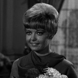
74 Appendix A 256 x 256 Images Aerial-1 Airplane Chemical Factory Clock Couple Girl-1 74

75 Girl-2 Girl-3 House Moon Surface Tree 75

76 512 x 512 Images Truck Aerial-2 76

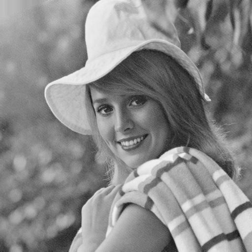
77 Car Elaine 77

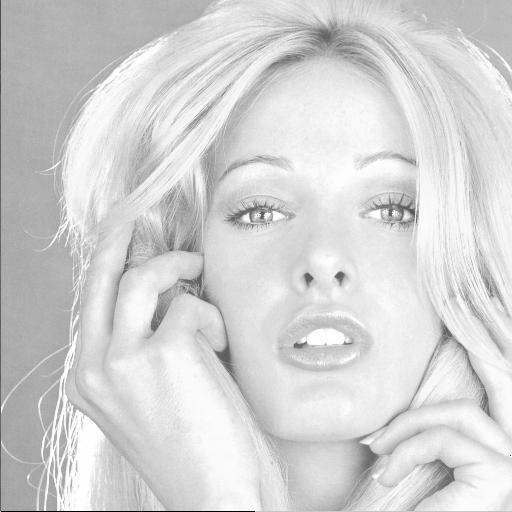
78 Fishing Boat Girl-4 78

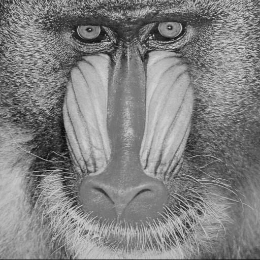
79 Lena Mandrill 79

80 Peppers Sailboat on Lake 80

81 1024 x 1024 Images Man 81

82 Airport 82