AFRL-RX-WP-TR

Transcription

1 AFRL-RX-WP-TR ADVANCED NONDESTRUCTIVE EVALUATION (NDE) SENSOR MODELING FOR MULTISITE INSPECTION R. Bossi, B. Koltenbah, L. Udpa, Yiming Deng, Liu Xin, Zhiwei Zeng, and Satish Udpa Boeing Phantom Works OCTOBER 2008 Final Report Approved for public release; distribution unlimited. See additional restrictions described on inside pages STINFO COPY AIR FORCE RESEARCH LABORATORY MATERIALS AND MANUFACTURING DIRECTORATE WRIGHT-PATTERSON AIR FORCE BASE, OH AIR FORCE MATERIEL COMMAND UNITED STATES AIR FORCE

2 NOTICE AND SIGNATURE PAGE Using Government drawings, specifications, or other data included in this document for any purpose other than Government procurement does not in any way obligate the U.S. Government. The fact that the Government formulated or supplied the drawings, specifications, or other data does not license the holder or any other person or corporation; or convey any rights or permission to manufacture, use, or sell any patented invention that may relate to them. This report was cleared for public release by the USAF 88th Air Base Wing (88 ABW) Public Affairs Office (PAO) and is available to the general public, including foreign nationals. Copies may be obtained from the Defense Technical Information Center (DTIC) ( AFRL-RX-WP-TR HAS BEEN REVIEWED AND IS APPROVED FOR PUBLICATION IN ACCORDANCE WITH ASSIGNED DISTRIBUTION STATEMENT. *//Signature// GARY J. STEFFES, Project Engineer Nondestructive Evaluation Branch Metals, Ceramics, & NDE Division //Signature// ALAN P. ALBERT, Maj, USAF Chief, Nondestructive Evaluation Branch Metals, Ceramics, & NDE Division *//Signature// ROBERT T. MARSHALL, Deputy Chief Metals, Ceramics, & NDE Division Materials and Manufacturing Directorate This report is published in the interest of scientific and technical information exchange and its publication does not constitute the Government s approval or disapproval of its ideas or findings. *Disseminated copies will show //Signature// stamped or typed above the signature blocks.

3 REPORT DOCUMENTATION PAGE Form Approved OMB No The public reporting burden for this collection of information is estimated to average 1 hour per response, including the time for reviewing instructions, searching existing data sources, searching existing data sources, gathering and maintaining the data needed, and completing and reviewing the collection of information. Send comments regarding this burden estimate or any other aspect of this collection of information, including suggestions for reducing this burden, to Department of Defense, Washington Headquarters Services, Directorate for Information Operations and Reports ( ), 1215 Jefferson Davis Highway, Suite 1204, Arlington, VA Respondents should be aware that notwithstanding any other provision of law, no person shall be subject to any penalty for failing to comply with a collection of information if it does not display a currently valid OMB control number. PLEASE DO NOT RETURN YOUR FORM TO THE ABOVE ADDRESS. 1. REPORT DATE (DD-MM-YY) 2. REPORT TYPE 3. DATES COVERED (From - To) October 2008 Final 10 February October TITLE AND SUBTITLE ADVANCED NONDESTRUCTIVE EVALUATION (NDE) SENSOR MODELING FOR MULTISITE INSPECTION 6. AUTHOR(S) R. Bossi, B. Koltenbah, L. Udpa, Yiming Deng, Liu Xin, Zhiwei Zeng, and Satish Udpa 5a. CONTRACT NUMBER FA C b. GRANT NUMBER 5c. PROGRAM ELEMENT NUMBER 62102F 5d. PROJECT NUMBER e. TASK NUMBER 41 5f. WORK UNIT NUMBER PERFORMING ORGANIZATION NAME(S) AND ADDRESS(ES) 8. PERFORMING ORGANIZATION REPORT NUMBER Boeing Phantom Works Boeing Information, Space & Defense Systems P.O. Box 3999 Seattle, WA SPONSORING/MONITORING AGENCY NAME(S) AND ADDRESS(ES) Air Force Research Laboratory Materials and Manufacturing Directorate Wright-Patterson Air Force Base, OH Air Force Materiel Command United States Air Force 12. DISTRIBUTION/AVAILABILITY STATEMENT Approved for public release; distribution unlimited. 13. SUPPLEMENTARY NOTES PAO Case Number: 88ABW ; Clearance Date: 11 Mar Report contains color. 10. SPONSORING/MONITORING AGENCY ACRONYM(S) AFRL/RXLP 11. SPONSORING/MONITORING AGENCY REPORT NUMBER(S) AFRL-RX-WP-TR ABSTRACT The Advanced Nondestructive Evaluation (NDE) Sensor Modeling for Multisite Inspection program has developed finite element models (FEM) of electromagnetic NDE for optimizing the inspection of aging aircraft structure. The program found excellent correlation between magnetic field strengths predicted by FEM analysis and experimental values in fastened airframe structure configurations. Applying the FEM analysis to magnetoresistive (MR) sensors inspection problems then provided useful insights into the many parameter effects associated with MR sensors, leading to optimized scanning predictions. The modeling and experimental analysis of the sensitivity of MR sensing for second layer cracks in thick (>0.16 inch top layer) structure demonstrated improvements in signal to noise by over an order of magnitude compared the currently applied conventional eddy current method. This result provided a quantitative evaluation of the MR sensor inspection method and validated the significant improvements in inspection capability that can be achieved in the MR mobile automated ultrasonic scanner (MAUS) implementation program. 15. SUBJECT TERMS nondestructive evaluation, electromagnetic modeling, giant magnetoresistive sensors 16. SECURITY CLASSIFICATION OF: 17. LIMITATION a. REPORT Unclassified b. ABSTRACT Unclassified c. THIS PAGE Unclassified OF ABSTRACT: SAR 18. NUMBER OF PAGES a. NAME OF RESPONSIBLE PERSON (Monitor) Gary J. Steffes 19b. TELEPHONE NUMBER (Include Area Code) N/A Standard Form 298 (Rev. 8-98) Prescribed by ANSI Std. Z39-18 i

4 TABLE OF CONTENTS Section iii Page Table of Contents iii List of Figures v List of Tables x Acknowledgements xi 1. Summary Introduction Aging Aircraft NDE Needs Electromagnetic NDE Modeling Electromagnetic Sensors Eddy Current Sensors GMR Sensor Advanced NDE Modeling Program Benefit Methods Assumptions Procedures Program Plan Literature Review Test Samples Model Development Introduction Geometry and Mesh Generation Interpolation/Shape functions and Global Matrix Assembly Boundary and Interface Conditions Matrix Solution Post-Processing Modeling GMR Probes with Induction Foil Excitation Results and Discussions MR Sensors Measurements MR Sensor Test System and Measurement Process Test Bed Scan System MR/MAUS System Demodulation Process Detection Angle Calibration Test Sample MR Data Subjective Data Analysis Tools and File Conversion Procedures C-Scans of S-2 Test Standard: Titanium and Steel Sides C-Scans of S-2 Test Standard: Frequency Variation Automated Defect Detection Amplitude-Based Features Shape-based features Classification Results Extension to multiple line plots... 63

5 4.2 Optimization of Parameters Through Modeling Model validation Model validation using notch calibration standard sample Model validation using S-2 Standard Sample Parametric Studies Introduction Frequency Effect Sensor Liftoff Effect Conductivity of Top Layer Effect Conductivity of Bottom Layer Effect Conductivity of Fastener Effect Fastener to Edge Effect Crack Dimension Effect Optimized Scanning Performance on New data from S2 sample Optimized Scan Conclusions Transition to MAUS Conclusions and Recommendations References APPENDIX A: Matlab Function Routines for MR Sensor Data Manipulation A.1 Introduction A.2 PostProcExtraction A.3 MRS_ReadSCDFile_ A.4 MRS_ExtractData_ A.5 MatlabExample A.6 Concluding Remarks APPENDIX B B.1 Introduction B.2 Running the Program B.2.1 Control Selection B.2.2 Load Data Button B.2.3 Save Image Button B.2.4 Function Selection B.2.5 Gradient Selection B.2.6 Detection Angle B.2.7 Color Scheme B.2.8 Data Z-Range B.2.9 X-Range (in) and Y-Range (in) B.2.10 Data X-Index Range and Data Y-Index Range B.2.11 X-Index Smoothing and Y-Index Smoothing B.2.12 Lighting B.2.13 Geometry B.3 Example B.4 Summary LIST OF ACRONYMS iv

6 LIST OF FIGURES Section v Page Figure 1 Experiment Setup with Conventional Eddy Current Testing... 7 Figure 2 MR Sensor Array with Sheet Current Excitation Foil... 7 Figure 3 Program Plan... 8 Figure 4 Program Schedule... 9 Figure 5 Notch Test Standard, inch-thick Aluminum with a 0.05 inch Wide Notch that is 0.25 inch Deep Figure 6 Leading Edge Part Figure 7 Leading Edge Figure 8 Wing Splice Standard Figure 9 Lower Wing Structure Standards Figure 10 Edge View of S-1 and S-4 Showing Thickness Difference Figure 11 S-1 Drawing Figure 12 S-2 Drawing Figure 13 S-3 Drawing Figure 14 S-4 Drawing Figure 15 Notch Sizes and Configurations Figure 16 Laboratory MR Sensor System Figure 17 Photographs of MR Sensors Attached to the MAUS V System Figure 18 Photographs of the New MR/MAUS System Under Development at Boeing St. Louis Figure 19 Plots from Boeing Seattle Test Bed System Figure 20 Plots of In-phase Demodulated Signal across the Calibration Standard of Figure Figure 21 Plots of S-2 Scan Figure 22 Analysis of the S-2 Titanium Side Cracks at f = 400 Hz and θ = 69.84º Figure 23 Analysis of the S-2 Steel Side Cracks at f = 400 Hz and q = 89.6º Figure 24 C-Scans of S-2 Test Standard at Various Frequencies Showing Titaniumside Inside-row Figure 25 C-Scans of S-2 Test Standard at Various Frequencies Showing Titaniumside Outside-row Figure 26 C-Scans of S-2 Test Standard at Various Frequencies Showing Steel-side Inside-row Figure 27 C-Scans of S-2 Test Standard at Various Frequencies Showing Steel-side Outside-row Figure 28 Peak Amplitude Definitions for Skewness Function Figure 29 Different Shape Information for Crack-free S-2 Sample Fastener Images Figure 30 Contour Pots for S-2 Smple Fastener Images at 400 Hz and DA = Figure 31 Illustration of 1-D Signal Extraction Figure 32 One-Dimensional Signals of Magnitude(blue), real(green), and Imaginary(red) Components Figure 33 Images of Fasteners with Different Crack Dimensions- (from top to bottom) 0.00 inch, 0.20 inch, 0.22 inch, 0.25 inch and 0.30 inch... 45

7 Figure 34 Parameter Definitions for inch Various Feature Extraction Figure 35 Two Dimensional Classification Results for S-2 Sample (0.16 inch Top Layer thickness) and Corresponding 1-D Signal Plots Figure 36 Two Dimensional Classification Results for S-4 Sample (0.25 inch Top Layer thickness) and Corresponding 1-D Signal Plots Figure 37 Estimation of Optimum Detection Angle Algorithm and Resulting Images for S-2 Titanium Outside Fasteners at 400 Hz Figure 38 Extraction of Line Plot from ODA Processed Images Figure 39 Line Plots for S-2 Ti Fasteners at 400 Hz Figure 40 Line plots for S-2 Steel Fasteners at 400 Hz Figure 41 Line plots for S-2 Ti Fasteners at Frequencies from 200 Hz to 400 Hz where Blue Lines are Defect Free Figure 42 Line Plots for S-2 Steel Fasteners at Frequencies from 200 Hz to 400 Hz where Blue Lines are Defect Free Figure 43 Classification Results for S-2 Ti Fasteners at Frequencies from 200 Hz to 400 Hz where Green Dots are Defect-Free Fasteners Figure 44 Classification Results for S-2 Steel Fasteners at Frequencies from 200 Hz to 400 Hz where Green Dots are Defect Free Figure 45 Illustration of the SNR Definition Figure 46 SNR Improvement after Applying ODA-based Method. SNR is Plotted Versus Crack Cross-sectional Area. The Points are also Labeled with Top Crack Dimension Figure 47 SNR Versus Frequency for S-2 Titanium Sample using MAG-based Method 61 Figure 48 SNR Versus Frequency for S-2 Titanium Sample using ODA-based Method 62 Figure 49 Line Plots and Scatter Plots in Two-Dimensional Feature Space for the Peak Occurring Position for S-2 Sample Titanium Fasteners Figure 50 Multiple Line Plots across a MR Sensor Fastener Image Figure 51 Collection of All Line Scans for Defect-free and Defective Inside Fasteners and Scatter Plot of Features Figure 52 Collection of All Line Scans for Defect-free and Defective Outside Fasteners and Scatter Plot of Features Figure 53 Collection of All Line Scans for Defect-free and Defective Fasteners Figure 54 Scatter Plot of Features for Multiple Lines Figure 55 Photographs of (a) the Sensor Head at the Zero-Balancing Calibration Position and (b) an Overhead View of the Calibration Sample with Slot Down the Middle. The Sensors and Excitation Current are Aligned Parallel to the Slot Figure 56 Sample Geometry Used in the Model Figure 57 (a) SidView and (b)top View of the Finite Element Mesh Figure 58 Modeling Results of the Normal Component of the Magnetic Flux Density (a) Real Part (b) Imaginary Part Figure 59 Geometry of Scan Plan Figure 60 Comparison of Demodulated and Calibrated Signal Across the Calibration Slot Figure 61 Geometry for S-2 Sample Figure 62 FE Mesh for S-2 Sample: (a) Side View (b) Top View Figure 63 Magnetic Flux Density for S-2 Sample Geometry in Figure 62 at 400 Hz (a) Magnitude (b) Real Component (c) Imaginary Component Figure 64 MRS Data for Crack-free Fastener in S-2 Sample at 400 Hz vi

8 Figure 65 Comparison between Experimental and Modeling Signal with Various Detection Phases Figure 66 Comparison between Experimental and Modeling Signal with Various Detection Phases Figure 67 Comparison between Experimental and Modeling Signal with Various Detection Phases Figure 68 Simulation Results for 100 Hz Frequency Figure 69 Simulation Results for 400 Hz Frequency Figure 70 Simulation Results for 0.5 khz Frequency Figure 71 Simulation Results for 0.7 khz Frequency Figure 72 Simulation Results for 2.0 khz Frequency Figure 73 Simulation Results for 7.0 khz Frequency Figure 74 Surface Plot of the Image Data Showing the Asymmetry in Two Lobes of Fastener Image Figure 75 Skewness Versus. Frequency for Results with 0.3-inch crack Figure 76 Simulated Line Scans at Different Frequencies for 0.3-inch Subsurface Cracks after ODA Processing Figure 77 Two-Dimensional Feature Space for Simulated Data at Different Frequencies Figure 78 SNR versus Frequency for Simulated Signal for S-2 Sample with 0.3 inch Subsurface Crack Figure 79 Bz Plots for inch Liftoff (a) Real, (b) Imaginary, (c) Magnitude Figure 80 Bz Plots for inch Liftoff (a) Real, (b) Imaginary, (c) Magnitude Figure 81 Bz Plots for inch Liftoff (a) Real, (b) Imaginary, (c) Magnitude Figure 82 Bz Plots for 0.1-inch Liftoff (a) Real, (b) Imaginary, (c) Magnitude Figure 83 Bz Plots for 0.15-inch Liftoff (a) Real, (b) Imaginary, (c) Magnitude Figure 84 Bz Plots for 0.2-inch Liftoff (a) Real, (b) Imaginary, (c) Magnitude Figure 85 Line Scans across the Center of Fastener of Real Part Figure 86 Line Scans across the Center of Fastener of Imaginary Part Figure 87 Mixed Line Scans Using ODA Figure 88 Peak Values of Real, Imaginary, and Mixed MR Signals Versus Liftoff Figure 89 Bz with 28% Iacs Top Layer Conductivity (a) Real, (b) Imaginary, (c) Magnitude Figure 90 Bz with 29% Iacs Top Layer Conductivity (a) Real, (b) Imaginary, (c) Magnitude Figure 91 Bz with 30% Iacs Top Layer Conductivity (a) Real, (b) Imaginary, (c) Magnitude Figure 92 Bz with 31% Iacs Top Layer Conductivity (a) Real, (b) Imaginary, (c) Magnitude Figure 93 Bz with 32% Iacs Top Layer Conductivity (a) Real, (b) Imaginary, (c) Magnitude Figure 94 Bz with 33% Iacs Top Layer Conductivity (a) Real, (b) Imaginary, (c) Magnitude Figure 95 Peak Value of the Signal Magnitude Versus Top Layer Plate Conductivity. 100 Figure 96 Bz with 30% Iacs Bottom Layer Conductivity (a) Real, (b) Imaginary, (c) Magnitude Figure 97 Bz with 31% Iacs Bottom Layer Conductivity (a) Real, (b) Imaginary, (c) Magnitude vii

9 Figure 98 Bz with 32% Iacs Bottom Layer Conductivity (a) Real, (b) Imaginary, (c) Magnitude Figure 99 Bz with 33% Iacs Bottom Layer Conductivity (a) Real, (b) Imaginary, (c) Magnitude Figure 100 Bz with 34% Iacs Bottom Layer Conductivity (a) Real, (b) Imaginary, (c) Magnitude Figure 101 Bz with 35% Iacs Bottom Layer Conductivity (a) Real, (b) Imaginary, (c) Magnitude Figure 102 Bz with 36% Iacs Bottom Layer Conductivity (a) Real, (b) Imaginary, (c) Magnitude Figure 103 Peak Value of the Signal Magnitude Versus Bottom Layer Plate Conductivity Figure 104 Real, Imaginary, and Magnitude of Magnetic Flux Density for Conductivity Values of Ti Fastener (1.0 percent Iacs, 2.2 percent Iacs, and 3.1 percent Iacs) as Indicated on the Left Figure 105 Real, Imaginary, Magnitude, Demodulated Bz for Fastener Edge Distance = 0.4 inch Figure 106 Real, Imaginary, Magnitude, Demodulated Bz for Fastener Edge Distance = 0.5 inch Figure 107 Real, Imaginary, Magnitude, Demodulated Bz for Fastener Edge Distance = 0.6 inch Figure 108 Real, Imaginary, Magnitude, Demodulated Bz for Fastener Edge Distance = 0.7 inch Figure 109 Real, Imaginary, Magnitude, Demodulated Bz for Fastener Edge Distance = 0.8 inch Figure 110 Line Scans Across the Center of the Fastener for Real Part of Bz Figure 111 Line Scans Across the Center of the Fastener for Imaginary Part of B Figure 112 Line Scans Across the Center of the Fastener for Mixed Signal Using ODA110 Figure 113 Edge Effect on Defect Signal Amplitude: Real, Imaginary, and Mixed Signals Versus Fastener-to-Edge Distance Figure 114 Bz for 0.2 inch Crack (a) Real, (b) Imaginary, (c) Magnitude Figure 115 Bz for 0.22 inch Crack (a) Real, (b) Imaginary, (c) Magnitude Figure 116 Bz for 0.25 inch Crack (a) Real, (b) Imaginary, (c) Magnitude Figure 117 Bz for 0.3 inch Crack (a) Real, (b) Imaginary, (c) Magnitude Figure 118 Bz for no Crack (a) Real, (b) Imaginary, (c) Magnitude Figure 119 Line Scans across the Center of the Fastener for Real Image Data Figure 120 Line Scans Across the Center of the Fastener For Imaginary Image Data Figure 121 Mixed Line Scans Using ODA of 70 Degrees Figure 122 Peak-to-peak values of Real, Imaginary, and Mixed MR Signals Versus Crack Area Figure 123 Peak-to-Peak Values of Real, Imaginary, and Mixed MR Signals Versus Crack Area Figure 124 Titanium Fastener Images for S-2 Test Standard at 400 Hz with ODA =70 degrees in Five Experimental Scans (a) to (e) Figure 125 Titanium Fastener Images for S-2 Test Standard at 650 Hz with ODA = 80 degrees in Five Experimental Scans (a) to (e) Figure 126 Collection of all Line Scans for Defect-Free (blue) and Defective (red) Fasteners viii

10 Figure 127 Scatter Plot of Features-Defect-Free (green), Defective (red) Figure 128 Scatter Plot of Features Defect-Free (green), Defective (red) Figure 129 SNR (Raw and Curve-Fitted) Plots Versus Frequency for S-2 Outside Fasteners Figure 130 SNR (Raw and Curve-Fitted) Plots Versus Frequency for S-2 Inside Fasteners ix

11 LIST OF TABLES Section Page Table 1 Publicly Released Reports from the Advanced NDE Sensor Modeling for Multi-Site Inspection Program... 2 Table 2 Air Force Supported Aircraft [2]... 3 Table 3 Advantages and Limitations of NDE Methods for Aging Aircraft... 4 Table 4 Representative List of Boeing Test Samples Options Table 5 Eddy Current Detection of Notches in Samples S-2 and S Table 6 Classification Results for S-2 Sample at 400 Hz and DA = Table 7 SNR Results Comparison for ECT, MAG, and ODA-Based Methods Table 8 SNR Values for Different Methods Table 9 SNR Values for Different Methods Table 10 Parameter Study Table Table 11 Peak-to-Peak Values of Bz for Various Sensor Liftoffs Table 12 Peak Values of Magnitude of Bz for Various Top Layer Conductivities Table 13 Peak Values of Bz Magnitude for Various Bottom Layer Conductivities Table 14 Effect of Fastener Conductivity on Peak Value of Magnitude Signal Table 15 The Peak-to-Peak Values Versus Fastener-to-Edge Distance Table 16 The Peak-to-Peak Values of Bz for Various Crack Dimensions Table 17 The Peak-to-Peak Values of Bz for Various Crack Dimensions (after Subtracting the Value Obtained for the Crack-Free Fastener) Table 18 SNR Values for S-2 Sample - Outside Fasteners at Different Frequencies Table 19 SNR Values for S-2 Sample - Inside Fasteners at Various Frequencies x

12 ACKNOWLEDGEMENTS The authors would like to acknowledge the vision and leadership of the AFRL Nondestructive Evaluation (NDE) Branch team of Tom Moran, Charles Buynak, Eric Lindgren, Jeremy Knopp, and Gary Steffes for their longtime support of the development of the magnetoresistive (MR) sensor inspection methodology. Paul Rutherford of Boeing Seattle is acknowledged for his support to the application and sample selection. Nancy Wood and Don Palmer of Boeing St. Louis are acknowledged for their contributions to MR sensor applications and scanning with the MR Mobile Automated Scanner (MAUS) system. xi

13 1. SUMMARY The Advanced NDE Sensor Modeling program has developed a finite element method (FEM) of electromagnetic NDE for optimizing the inspection of aging aircraft structure. The significant results of the program include 1) excellent correlation of electromagnetic FEM predictions with MR sensor experimental data for aircraft fastened structure configurations, 2) evaluation of parameter variation that affect the signal to noise in the resulting data, and 3) optimized MR scanning of test samples showed an improvement in sensitivity to second layer flaws by over an order of magnitude compared to standard eddy current inspection. MR sensors are found to provide robust signals of the magnetic field strengths in electromagnetic testing. The data, however, can be subject to interpretation difficulties due to the field patterns from geometric features. The FEM approach accurately represented the fields and response of MR sensors from AC currents induced in metal geometries for cracks near fasteners in the second layer under thick (>0.16 inch) skins. Once satisfactorily calibrated, the model was used to conduct a variety of parametric studies including frequency, sensor liftoff, conductivity of layers, fastener to edge distance and crack dimension. Additionally, meticulous analysis of MR sensor measurements was performed to development automated feature recognition. The data was further processed to place an objective value to cracks as they appear in MR sensor data. As a result of quantitative data reduction, it has been possible to establish a signal-to-noise ratio (SNR) value for the MR sensing. With this evaluation it was possible to show that MR sensors offer considerable value over conventional eddy current inspections with the possibility of improvements in sensitivity by over an order of magnitude. The results of this program validate the importance of MR sensors for deep, second layer inspections in aging aircraft and should lead to cost savings through reduced teardown and faster inspection at improved sensitivity over presently applied methods. Further efforts are warranted to enhance the usefulness of MR sensors through reverse modeling for sizing, evaluation of a greater number of parametric effects that could not be covered in this program, and investigating MR sensor orientation and geometry variations. In addition to this final report, the program has generated several publicly released reports as listed in Table 1. 1

14 Table 1 Publicly Released Reports from the Advanced NDE Sensor Modeling for Multi- Site Inspection Program Title/Authors Automated Analysis of Eddy Current Giant Magnetoresistive Data, Y. Deng, X. Liu, Z. Zeng, B. Koltenbah, R. Bossi, G. Steffes, and L. Udpa, GMR signal analysis for Detecting Cracks Under Fastener Heads in Multilayer Aircraft Structures, Z. Zeng, Y. Deng, X. Liu, L. Udpa, S. S. Udpa, B. Koltenbah, R. Bossi, and G. Steffes Feature Based Analysis of Magnetoresistance Sensor Data for Nondestructive Testing Applications, Y. Deng, X. Liu, Z. Zeng, B. Koltenbah, R. Bossi, G. Steffes and L. Udpa Electromagnetic Modeling of Magnetoresistive Sensors, B. Koltenbah, R. Bossi, G. Steffes, L. Udpa, Y. Deng, X. Liu and Z. Zeng Publication Review of Progress in Quantitative Nondestructive Evaluation, (28)2008 (Inpress) IEEE Transactions on Magnetics (under review) 13th International Workshop on Electromagnetic Nondestructive Evaluation, Korea, 2008 ASNT Fall Conference and Quality Testing Show, Las Vegas, Nov INTRODUCTION 2.1 AGING AIRCRAFT NDE NEEDS The development of NDE methods is vital in determining the state of health of aging aircraft materials. With continuing reductions in new weapons systems procurements, there has been and continues to be a need to increase the service life of aircraft currently in the Air Force inventory. This requirement has made the detection and characterization of corrosion and cracking a major Air Force logistics needs. Table 2 shows a listing of several types of Air Force aircraft and their average age [1,2]. Design lifetimes for these aircraft are typically 20 to 30 years. Some of the aircraft referenced in Table 2 have more than exceeded their design lifetimes. In fact, the current strategies include extending the service lives of aircraft such as the B-52 and KC-135 up to 80 years. 2

15 Aircraft Type Number of Aircraft Table 2 Air Force Supported Aircraft [2] Average Age (Years) Comments A Retain 25+ years no replacement identified [1] B-1B B No replacement identified C C C E E F-15 C-D Retire replace with F-22 F-15 E F Retire replace with Joint Strike Fighter (JSF) KC KC Replacement over time with some aircraft reaching 80 years T T For aging aircraft inspection the inspection technique needs to be readily fieldable, onesided, applicable to variable materials and geometries, and sensitive to defects in sublayers. Table 3 compares the advantages and limitation of the general categories of NDE methodologies. Of these methods, it is evident that the emphasis of study for aging aircraft NDE should be the eddy current method because it is the only approach that is relatively low cost, one-sided, and has the ability to penetrate multiple layers. Eddy current NDE methods create electromagnetic fields through some form of alternating current flow. These fields penetrate into the aircraft material and induce eddy currents, which themselves generate a responding electromagnetic field. The superposition of these electromagnetic fields is then measured. Changes in the electromagnetic field can be readily detected by the eddy current device provided the detector has sufficient sensitivity. Standard eddy current testing (ECT) methods using wound coils, however, suffer from limitations due to the principles of coil technology for frequency of operation and physical size. This results in significant limitations in sensitivity as a function of depth of penetration for sublayer defect detection. Lower frequencies required for penetration use large coils which decrease resolution. These limitations can be overcome by using advanced electromagnetic sensors and modeling studies to improve the detection sensitivity to meet aging aircraft inspection needs. 3

16 Table 3 Advantages and Limitations of NDE Methods for Aging Aircraft NDE Methodology Advantages Limitations VT - visual and/or Low cost, Surface only Enhanced Visual Easy to implement For subsurface requires invasive Testing measures ET eddy current testing UT ultrasonic testing RT radiographic testing IRT thermographic testing PT and MT penetrant and magnetic particle One sided Low cost Multi-layer sensitivity One sided Low cost Multi layer sensitivity High resolution Image display Non-contact One sided Low cost Sensitivity at depth Interpretation of signals First layer (marginal or no sensitivity to second layer) Couplant required Two sided Backscatter technique for onesided is too slow and lacks sensitivity to small defects First layer, no known sensitivity to second layer features First layer only for surface or near surface defects 2.2 ELECTROMAGNETIC NDE Electromagnetic NDE, especially in the form of ECT, is the most widely used inspection method for metallic aircraft inspection. Of paramount importance is the sensitivity of the electromagnetic methods to aging aircraft defects in multilayered geometries. As noted above, ECT suffers from limitations for detecting defects in multilayer complex structure configurations due to the coil size required for the penetrating frequencies of operation in thick structure. The standard eddy current method easily becomes limited in sensitivity as a function of the depth of penetration. This is fundamental to the physics of the electromagnetic field problem and the interactions of the induced currents with the materials and defects, and the interaction of the altered fields with the sensors. Advanced electromagnetic sensing methods, such as MR sensors, have been developed that offer significant advantages over traditional ET sensors for sensitivity at depth. The Air Force Research Laboratory NDE Branch funded a series of programs to develop MR sensors into useful tools for the in-service inspection of at aircraft that would provide improved capability over currently applied methods [3,4,5]. However, the implementation of MR sensors is subject to a great number of variables when applied to multi-site geometric configurations 4

17 and defect types. These include variables due to the method, such as frequency, beam size, excitation, sample spacing, etc., variables due to the object such as materials, sizes, shapes, configuration, edges, gaps, etc. and variables due to the defects such as length, width, volume, shape, distribution, orientation, etc. All three sets of variables will be combined in any inspection causing uncertainty in the interpretation of the signals. The result is that the sensitivity to defect types, sizes and orientations is rarely optimized. Intuitive or empirical approaches to optimize the inspections are inefficient and expensive because of the large number of variables that affect the sensitivity. By employing modeling of the electromagnetic field generation and the interaction of the fields with materials, geometries, features and sensors the electromagnetic NDE sensitivity can be assessed and inspection parameters optimized efficiently. Modeling of the physics problem provides the best approach for optimization and will result in improved probability of detection (POD) based on how each kind of sensor system will behave for a given geometry, excitation method, crack or corrosion size, and orientation. 2.3 MODELING Electromagnetic modeling has also been under development and studied for a number of years, particularly at Michigan State University (MSU) for NDE applications and at Boeing for general physics problems. Models can be broadly classified as either analytical or numerical. The early work of Dodd and Deeds, who derived closed form integral expressions for the impedance of a coil placed above a layered half-space conducting medium, set the stage for the development of a series of models characterizing eddy current NDE phenomena [6]. Although these models continue to be used extensively to this day, a number of extensions have been proposed in recent years using volume integral and boundary integral methods. However, such analytical models are, in general, limited in their application to simple specimen and defect geometries. Numerical models have gained popularity in recent years due to their ability to simulate arbitrary-shaped defects in complex sample geometries. Numerical models can help in visualizing the electromagnetic field distribution and the manner in which the field interacts with the flaw in the test specimen. Such models can be used to conduct systematic parametric studies as the material, defect and experimental parameters are varied. The knowledge of the qualitative and quantitative influence of these parameters on the sensor measurement can be useful in determining improvements needed in sensor and system design and for maximizing the probability of detection (POD) of critical flaws in structures. Numerical models can also serve as a test bed for generating defect signatures for a variety of defects. These defect signatures can be employed for developing inversion algorithms as well as for training inspection personnel. Finally, computational models can be used to explore the feasibility of novel inspection methods and evaluate new types of sensors. 5

18 2.4 ELECTROMAGNETIC SENSORS Eddy Current Sensors Eddy current NDE techniques are based on the principles of electromagnetic induction. These techniques find widespread use for inspecting aircraft structures largely due to their noncontact nature, simplicity of operation and sensitivity to anomalies in thin multilayer conducting structures. The basic eddy current probe consists of a coil excited by an alternating current source. When the probe is brought in close proximity to a conducting sample, eddy currents are induced in the test specimen. The secondary field generated by the induced currents alters the net flux linkages associated with the probe coil. This change in flux linkages is reflected as a change in the terminal impedance of probe. The impedance change of the probe coil, as the sample is scanned, constitutes the eddy current signal. Coil type transducers offer the advantages of being very accurate, robust and simple to construct. Unfortunately, the measurements tend to be somewhat noisy since the output voltage is related to the time-derivative of the field. However, this is seldom a concern in the case of conventional single frequency eddy current methods, since the coherent detection scheme employed in most eddy current instruments offers excellent noise rejection characteristics. Major issues in eddy current inspection include the limited depth of penetration and the challenges involved in interpreting the complex probe impedance signal. Eddy current inspection systems have grown in sophistication with advancements in the fields of sensors, microelectronics and computers. Concurrently, advancements in our ability to model the underlying physical processes give us the ability to develop novel probe designs [7]. Sensors that measure the field due to induced currents directly as opposed to coil sensors that measure the derivative of the field are attracting attention. Giant magnetoresistive (GMR) probes [8,9], Hall sensors, fluxset probe [10], magneto-optic sensors [11,12] and meandering wire magnetometers [13] are all examples of sensors being considered seriously as alternatives to the classical eddy current coil. Advantages offered by these sensors range from high levels of sensitivity to small size GMR Sensor Among sensors that are capable of measuring the field due to induced currents directly, GMR probes appear to be the most promising. These probes offer exceptional levels of sensitivity, small size and low cost. A simple GMR probe configuration is shown in Figure 1, where the excitation coil encircles the GMR sensor [14]. The magnetic field generated by the excitation coil induces currents in the specimen. The induced currents are distorted if a crack is encountered. The GMR sensor picks up perturbations in the fields associated with the induced eddy currents. Signal processing algorithms may be required to demodulate the signal detected by the GMR sensor. 6

19 Figure 1 Experiment Setup with Conventional Eddy Current Testing Figure 2 shows an alternative approach to using the GMR sensor where the sinusoidal excitation current is applied to an induction foil. An array of GMR sensors can be used to pick up the normal component of magnetic flux density generated by the induced currents. In the absence of any discontinuity, the magnetic flux is tangential to the specimen surface resulting in a null signal. Anomalies in the specimen result in a normal component of the magnetic flux density. The normal component of the magnetic field is sensed by the GMR sensor. Alternately, a pulse excitation current can be applied to the induction foil and an array of GMR sensors can be used to measure the transient magnetic field at different locations simultaneously. The output signals from the GMR sensor array contain time and space information. The information can be used to estimate the defect depth and location. Figure 2 MR Sensor Array with Sheet Current Excitation Foil 2.5 ADVANCED NDE MODELING PROGRAM BENEFIT The Advanced NDE Sensor Modeling for Multisite Inspection program was a three year effort concentrated on the development of appropriate electromagnetic models suited to MR sensors to determine the optimum sensitivity capability. The investigation modeled standards that represent damage situations identified in the Air Force and at Boeing as serious concerns involving cracking in sublayers of thick (>0.25 inch) metallic structure. Testing and correlation of real data with modeled data was performed to validate and improve the modeling. The verified models were used to predict the optimum parameters for MR inspection of simulated aging aircraft structure configurations. The influence of the complexities of aging aircraft inspection, such as multiple layers, thickness variations, gaps, material changes, defect size and defect orientation were examined and analyzed by the modeling studies. The improvement in defect detection and sizing, through the use of advanced sensors with optimized model predicted inspection parameters, was assessed compared to conventional eddy current and found to be about an order of magnitude better. 7

20 3. METHODS ASSUMPTIONS PROCEDURES 3.1 PROGRAM PLAN The program plan for Advanced NDE Sensor Modeling for Multi-Site Inspection, is shown in Figure 3. The program schedule is shown in Figure 4. The program involved the cooperative efforts of Boeing Phantom Works and MSU Electrical and Computer Engineering Department. Boeing, MSU and the Air Force set the direction of the program beginning with a kickoff meeting in February of At that time the electromagnetic methods, test sample configuration and modeling code approaches were selected. Task Literature Review and Tasks and 1.1.3, Test Samples and Model Development, are discussed in sections 3.2, 3.3 and 3.4 of this report. Section 4 of the report discusses the results of Tasks 1.2, 1.3 and 1.4. Advanced NDE Sensor Modeling for Multi-Site Inspection Program Plan Task 1.5 Kick-off Meeting (AF, Boeing, MSU) Tasks & Task 1.2 Selection of Modeling Inspection Code Activity Methodology, for MR, EC Modeling Code and PEC Approaches and Sensors Test Sample (MSU) Configurations (MSU, Boeing, AF) Task Task Correlation Evaluate of Real Sensitivity of Data with Optimized Models and Parameters for Optimize Inspection on Test Code Sample (MSU) Configurations (MSU) Task Literature Review on Modeling (MSU) Task 1.3 Task Task 1.5 NDE Data Test Optimized Final Acquisition on Parameters and Report Control Estimate (MSU, Standards using Improved Boeing) Advanced Probability of Electromagnetic Detection Sensors (Boeing) (Boeing) Figure 3 Program Plan 8

21 Figure 4 Program Schedule 3.2 LITERATURE REVIEW Computational methods for modeling electromagnetic NDE problems fall into two major classes, namely, analytical and numerical approaches. Analytical models are capable of providing ideal, closed form solutions to problems. However, such analytical models are, in general, limited in their application to simple specimen and defect geometries, such as infinite half plane samples and regular, rectangular or hemispherical crack geometry. Numerical models have gained popularity in recent years due to their ability to simulate arbitrary shaped defects in complex sample geometries. Numerical models can simulate problems with high dimensionality as well as nonlinear, anisotropic and inhomogeneous material properties. With the development of faster and more powerful computers, the development and implementation of the numerical models have become a major research focus in NDE [15,16]. Several numerical modeling methods have been developed for solving the governing equations describing various NDE phenomena, such as finite difference method (FDM), FEM, boundary element methods (BEM), boundary integral methods (BIM) and volume integral methods (VIM). Each method has its own advantages and limitations and is appropriate for different kinds of numerical problems [10,17,18,19]. The finite difference method is the simplest numerical modeling method for solving partial differential equations (PDE). The advantage is its relative ease and intuitive method for approximating partial derivatives by corresponding finite difference formulation. It is widely applied for direct current, quasi-static, transient fields, and linear problems. A 9

22 limitation of the finite difference technique is its poor convergence property, particularly in the case of irregular geometries. Also, finite difference formulations do not lend themselves easily for modeling distributed parameters such as the current densities, conductivities and permeability [14]. FEM evolved in the late 1950s as a numerical technique in structural analysis and was quickly adapted as a major numerical modeling method in various engineering fields to solve PDE. The finite element domain discretization scheme allows modeling of complex shapes, making it efficient and relatively more accurate [10]. Compared with FDM, FEM has many advantages including its ease of imposing essential boundary conditions and modeling complex geometries. FEM formulations can be easily extended to handle higher order approximation and thereby lead to faster convergence and better accuracy. The resulting matrix equations are in general sparse, banded and diagonally dominant making the solutions process very stable [12]. FE models have been developed and used for a variety of two- and three-dimensional eddy current NDE problems [20,23 ]. The drawbacks of FEM include large computer resources especially for nonlinear and time-dependent problem. Also, the finite element method is not well suited for open region problems [12] encountered in wave regimes. In the area of antenna and electromagnetic wave propagation, integral equation based approaches are more commonly used. BEM and VIM methods based on the integral equations [12,13] along with absorbing boundary conditions are typically used in wave propagation problems where the Green s function is readily available. Boundary integral methods solve Maxwell s equations by integrating the appropriate Green s function over the boundary using the given boundary conditions. Hence there is a need to discretize only the boundary surface in the integral equations, rather than calculating all values in solution domain. In the post-processing phase, the integral equation is used again to calculate the required physical quantity at any point in the solution domain. In the case of inhomogeneous problems, VIM is commonly applied to discretize the volumetric source for solution. In VIM, the field is determined at a point by summing the effects of the sources at all points. The volume integral computes a convolution of the source points with the appropriate Green s function. The advantage is it is only necessary to construct a mesh over the test sample and solve for the currents in the test sample. But this method also requires computation of the Green s function which in itself may not be trivial. Integral equation based formulation is in general more efficient than differential equation model with regard to computer resources but the resulting global stiffness matrix equation is generally fully populated and ill conditioned, leading to instabilities [21]. More importantly VIM and BEM are inherently linear and can be used to solve linear homogeneous problems. Lastly these methods are useful only when the Green s function for the problem is easily available. In this project, we use the finite element method for modeling the multilayered geometry largely due to the ease of modeling ferritic and nonferritic fasteners and complex defect shapes, as well as the inherent stability and accuracy of the solution procedure. 10

23 3.3 TEST SAMPLES In this program, where modeling will be used to predict and optimize performance, test standards play a vital role. The test samples need to be well suited for model development yet representative of the aging aircraft issues facing the Air Force. Figure 4 lists some of the test sample considered for this program and Figure 5 through 10 are photographs of the various samples. Calibration Standard Table 4 Representative List of Boeing Test Samples Options Sample Size Description Leading Edge Part Leading Edge Spar Wing Splice Standard Lower Wing Structure Standards 20 x 13 x 1 inch inch-thick aluminum plate with notch Leading edge structure Leading edge spar Lower Structure 12 x 4 inch W-67 configuration 0.5 inch aluminum with 0.25 inch double lap splice Four samples: S-1, S-2, S-3 and S-4 representative of 707 type center wing tank structure inspection Figure 5 Notch Test Standard, inch-thick Aluminum with a 0.05 inch Wide Notch that is 0.25 inch Deep 11

24 Figure 6 Leading Edge Part Figure 7 Leading Edge Figure 8 Wing Splice Standard 12

25 Figure 9 Lower Wing Structure Standards Figure 10 Edge View of S-1 and S-4 Showing Thickness Difference Of these samples, the criteria for being suitable to model and representative of a critical Air Force need focused on the W-67 location on KC-135 (Boeing 707 type) aircraft center wing box structure configuration of samples S-1, S-2, S-3 and S-4 provided by Paul Rutherford [21]. Currently standard eddy current inspection is used on these samples. These standards represent a splice with four rows of fasteners and two rows on each side of the splice. The fasteners are titanium on one side of the splice and steel on the other. S-1 and S-2 have 0.16 inch top layers while samples S-3 and S-4 have 0.25 inch top layers. Edge views of S-1 and S-4 are shown in Figure 10. The bottom splice plate is inch thick. Notches have been inserted at the fastener holes. Figure 11 through 14 show the layout and section 13

26 cuts for the four samples. Figure 15 shows the notch defect size and configuration in the samples. The notch configurations were triangular including 0.10 inch length by 0.13 inch depth, 0.13 inch length by 0.17 inch depth, 0.15 inch length by 0.2 inch depth, 0.17 inch length by 0.22 inch depth for S-1 and S-3 and 0.2 inch length by 0.26 inch depth, 0.22 inch length by 0.29 inch depth, 0.25 inch length by inch depth and 0.30 inch length by inch depth for S-2 and S-4. Table 5 shows the results of eddy current inspection on the S-2 and S-4 samples. The signal to noise is interpreted by the operator, where values of 1 indicate that the defect cannot be detected. In general the standard eddy current inspection is not sensitive in the second layer to notches less than 0.25 inch in length. Figure 11 S-1 Drawing 14

27 Figure 12 S-2 Drawing Figure 13 S-3 Drawing 15

28 Figure 14 S-4 Drawing Figure 15 Notch Sizes and Configurations 16

29 Table 5 Eddy Current Detection of Notches in Samples S-2 and S MODEL DEVELOPMENT Introduction The FEM is one of the most widely used tools for analysis. The method finds applications in diverse areas of engineering and science largely due to its ability to model intricate geometries efficiently and accurately. In the last few decades, FEM has been applied with great success in such areas as the study of DC and low frequency electromagnetic fields in electrical machines, design of structures, modeling thermal fields and NDE. The FEM was selected for this project to provide an accurate and robust simulation of the electromagnetic fields. A formulation of the problem from first principles derived from Maxwell s equations governing the differential equations to be solved in the model is provided by Jin [22] and shown in Equations (1) to (7). Two- and three-dimensional electromagnetic finite element models for electromagnetic NDE applications have been developed over the last two decades and used extensively by the MSU team. Examples of successful modeling efforts include twoand three-dimensional eddy current models for simulating steam generator tube inspections [23], three-dimensional magneto-static model for simulating gas transmission pipeline inspection [24] and three-dimensional modeling magneto-optic imaging inspection [25]. More recent work comprises a three-dimensional model for microwave inspection of re-bars in concrete structures [26]. The major steps in FEM are described briefly below. The Maxwell s equation in differential form are given by B E = (1) t D H = J s + J + (2) t B = 0 (3) 17

30 D = ρ, (4) With the constitutive relations: B = µh (5) D = εe (6) J = σe. (7) In Equation (1) through (7), E = electric field intensity (volts/meter) D = electric flux density (coulombs/square meter) H = magnetic filed intensity (amperes/meter) B = magnetic flux density (webers/square meter) J s = source current density (amperes/square meter) J = conduction current density (amperes/square meter) ρ = electric charge density (coulombs/cubic meter) µ = permeability (henrys/peter) ε = permittivity (farads/meter) σ = conductivity (siemens/meter). The vector potential formulation, A-V Formulation is used for this project. From (3), the magnetic flux density is divergence free and can be expressed as the curl of a vector, i.e., B = A, (8) where A is the magnetic vector potential. The magnetic field intensity can also be expressed in terms of A, as 1 H = A µ (9) Substituting (8) into the Faraday s Law (1), we get 18

31 A E = (10) t A E + = 0 (11) t Then the electric field intensity can be expressed as E = jω A V (12) The j ω term is introduced since we are dealing with the time-harmonic problems for this project. Equation (12) tells us that the electric field intensity E can be expressed in terms of the magnetic vector potential A and the scalar function V Geometry and Mesh Generation The test geometry truly simulated is that of the S2 sample as described in Section 3.3. It consists of two layers of aluminum. The top layer is 0.16 inch thick and the bottom layer is inch thick. The sample contains a top layer and second layer edges close to the fastener. Notches are introduced at the fastener holes as shown in Figure 15. The threedimensional domain is discretized using brick or hexahedral elements interconnected at eight nodes. The mesh size and complexity increases particularly when a small air gap of inch is introduced between the layers and also between the fastener and plate. The density of mesh elements were optimized and validated by comparing the model prediction with experimental measurements Interpolation/Shape functions and Global Matrix Assembly The magnetic vector A and electric scalar potential V in an element e is expressed in terms of selected linear or quadratic interpolation functions as follows 8 24 e e e e e e e e e A = N A j xj xˆ + N j Ayj yˆ + N j Azj zˆ = N k Ak (13) j= 1 k = 1 8 e e e V = N V, (14) j= 1 j j where e N xˆ j k = 3 j 2 e e N = N yˆ k j k = 3 j 1, (15) e N j zˆ k = 3 j 19

32 and A e k A = A A e xj e yj e zj k = 3 j 2 k = 3 j 1, (16) k = 3 j where A xj, A yj, A zj and V j are the three Cartesian components of the vector potential and the scalar potential at node j; and N j is the shape function associated with node j that assumes the value of one at this node and the value of zero at any other node. The vectors xˆ, yˆ, zˆ are the Cartesian unit vectors. obtain Using the Galerkin formulation [27], and imposing the Coulomb gauge on (8) and (12), we 24 { j= 1 Ωe 1 ( N µ e i ) ( N e j 1 ) + ( N µ e i )( N e j ) dv} A e j + 24 e e e { jωσ N N dv} A + { Ω i j j e j= 1 j= 1 8 Ωe σn e i N e j dv} V e j Ω e for i = 1,2,, 24 e 1 e e 1 e N i ( A nˆ) ds Ni ( nˆ A ) ds = µ Ω e µ 24 e e e { jωσ N N dv} A + { Ω k j j e j = 1 j = 1 8 Ωe σ N e k Ωe N e j e N J dv, (17a) e i dv} V s e j + Ω σ N e ( ) ˆ k jωa V nds = 0, (17b) e for k = 1,2,, 8 where nˆ is the outward unit vector and Ωe is the boundary of the subdomain Ω e. Combining these equations together, we obtain a matrix equation, e e e [ G ] [ U ] = [ Q]. (18) e The global stiffness matrix is obtained by assembling each element matrix [ G] together. The value at each entry is the sum of values contributed by all the connected elements: GU = Q, (19) 20

33 where G is a complex, symmetric sparse matrix, U is the vector of unknowns consisting of the electric scalar potential and the three components of the magnetic vector potential at each node and Q is the load vector incorporating the current source Boundary and Interface Conditions To obtain a unique solution, appropriate boundary conditions need to be imposed before solving the system of equations. Either Dirichlet boundary conditions (values of A or V on the boundary) or Neumann boundary conditions (values of the magnetic flux density B or the magnetic field intensity H on the boundary) need to be specified. Since Neumann boundary conditions are usually included implicitly in the finite element formulation, we only need to impose Dirichlet boundary conditions. Current continuity conditions will be explicitly imposed at the interface boundaries to avoid spurious solutions Matrix Solution The finite element procedure results in a linear algebraic system of equations that must be solved to determine the unknown coefficients of the shape functions. The equations can be solved using either direct or iterative methods. The Gaussian elimination method is a direct approach that can be used to solve either full or sparse matrix equations. In the finite element method, the stiffness matrix is usually sparse and banded. In such cases, it is more advantageous to employ iterative methods since they are more efficient with respect to computational cost and data storage. A number of iterative methods have been proposed over the years. However, only a small number of them can be used for solving the complex-valued matrix equations arising in quasi-static electromagnetic problems. We propose to use the Transpose Free Quasi-Minimal-Residual (TFQMR) method [28] where the associated Krylov 2 n 1 subspace is Kn span{ Q, GQ, G Q,, G 1 = Q}. The exact solution U = G Q could be approximated by Un Knthat minimizes the norm of the residual r n = Q GU n. The TFQMR algorithm relaxes this minimization requirement. It aims to minimize a different, datadependent norm that in practice is similar to r. An important issue in iterative methods is its convergence properties. The convergence of iterative process depends on the properties of the matrix, such as its eigen values, the singular value or condition number. Usually a large condition number will result in a large solution error or sometimes even failure to converge. Thus, the process of preconditioning is essential for the success of iterative methods. The overall solution procedure requires O (N) multiplications and additions [29] Post-Processing After we solve for the potentials, physical and measurable quantities of interest, such as the magnetic flux density B, coil impedance and induced current density J, can be calculated using: B = A (20) n E = jω A V (21) 21

34 J E, (22) where Equations (20) through (22) are the same as Equations (8), (7) and (12) and presented here again for the reader s convenience. GMR sensors measure the normal component of the magnetic flux density B. The different components of the magnetic flux density can be obtained from the nodal values of magnetic vector potential as: A A z y Bx (23a) y z B B y z Ax Ax z x (23b) Ay Ax. x y (23c) The current density J inside element e is determined at the element center from the relation e 8 8 e e e V e e N i e J x j Ax j N i Axi Vi. (24) x x i 1 i 1 The components e J y and e J z can be calculated similarly Modeling GMR Probes with Induction Foil Excitation The excitation source in this project is applied to an infinite planar induction foil located parallel to the surface of the specimen. For a linear sinusoidal current excitation with angular frequency of, the source current is j lin, j t Re[ J0e ] J0 cos t (25) where J 0 is the magnitude of the current. However a probe with a linear excitation current flow pattern is sensitive only to cracks that are perpendicular to the current direction. In this project, to best detect a crack oriented in the x direction the current flow is assumed to be along the y direction, i.e., Jlin yˆj 0 where ŷ is the unit vector along the y-axis. The normal component of magnetic flux density Bz will be measured by the GMR sensor array. 22

35 4. RESULTS AND DISCUSSIONS 4.1 MR SENSORS MEASUREMENTS MR sensor measurement and data analysis have been of major focus throughout Boeing s development history of this technology [3,4,5]. Although MR sensing techniques are similar to and are based upon eddy current measurement methods, the MR sensor measurement and data processing methods have evolved to be distinct and unique from traditional eddy current technology. This distinction is enough to classify MR sensors as a new modality of electromagnetic NDE with unique advantages over eddy current for particular measurement needs. This uniqueness, however, requires the establishment of new calibration and measurement techniques as well as new data interpretation methodologies and advanced feature extraction algorithms. In support of this program, measurements were taken at both the Boeing Phantom Works Physics NDE Laboratory in Seattle using the MR Sensor Test Bed Scan System and the Boeing Phantom Works MR Sensor/MAUS Scan System in St. Louis. The Seattle-based measurements were used initially to validate and calibrate MSU modeling results. Following this, the measurements were used in both the development and testing of advanced feature recognition and signal to noise (SNR) extraction algorithms at both Boeing and MSU. Section 4.1 is organized as follows: Section details the MR sensor test systems developed by Boeing and used in this program. Section presents the MR test sample data in support of the modeling and feature extraction efforts. Section presents the algorithms developed for and the results of SNR extraction from the measurement data MR Sensor Test System and Measurement Process This section presents the MR Sensor test systems and measurement processes. The existing MR systems at Boeing Phantom Works include a prototype Test Bed Scan System unit and the MAUS-based system presently under development. Both are capable of accomplishing this task of producing measurement data in support of the modeling and data analysis efforts of this program. The laboratory-based unit was used for taking most of the experimental test data. The measurement process for the Test Bed Scan System is detailed below Test Bed Scan System The Test Bed Scan System (shown in Figure 16) consists of the following major components: (1) MR Sensor Head, (2) PXI Chassis, (3) XY Scan Bridge, and (4) Executive Computer. 23

36 Figure 16 Laboratory MR Sensor System The MR Sensor Head consists of one MR sensor card with a linear array of 32 GMR sensors arranged in a row 1 inch in length (see bottom-right picture in Figure 16). The sensors (and card) are aligned normal to the scan/index plane (the z-direction) such that a 1 inch swath is swept by the sensors along the scan direction (the x-direction). The card includes cable connectors for the sensors. The MR Sensor Head is housed in a metal box for shielding (see upper-right picture in Figure 16). At the bottom of the head is a shoe to which a copper foil is adhered. This foil contains strips that deliver a linear, unidirectional excitation current. The direction of current is along the line of sensors, which is along the index direction (the y-direction). The Sensor Head also contains hardware for a DC strip current. This strip current is provided to shift the operating point of the MR sensors such that they are optimized for maximum sensitivity along the most linear portion of their magnetic field to current response curves. The PXI Chassis contains both Boeing-developed hardware for excitation signal source, strap current and encoder signal processing and off-the-shelf hardware components for both D/A and A/D conversion of sensor signals and digital control of various system components. The latter tasks are accomplished through five multifunction cards from National Instruments. A voltage output channel (D/A converter) of one card is used to seed the AC excitation signal for desired amplitude and frequency. This excitation signal is pre-processed in the Boeing hardware, which is housed in one slot of the PXI chassis and uses the PXI power supply bus. The excitation signal is connected through cable to the excitation sheet at the bottom of the MR Sensor Head. Thirty-two of the available voltage input channels (A/D converters) are used to input the return signals from the sensors, which are first pre-processed through amplifiers on the Boeing hardware. In addition to these 32 signals, two input channels are devoted to reading and digitizing the excitation signal and its quadrature signal in the same manner as the sensor signals. 24

37 The XY Scan Bridge (upper left picture of Figure 16) allows for accurate position and motion control within 0.01 inch (and theoretically even smaller) in both in-plane directions. The position and scan speed of the MR sensors can therefore be controlled to adequate precision to produce high resolution c-scans. The Executive Computer controls the PXI Chassis through a connected PC-card / PXIcard interface. Control software is written in LabVIEW to provide extensive graphical interface and control. C-scan data is saved in a specialized scan data file format (.SCDextension). A converter program has been developed to read and parse the full SCD data format into the Matlab programming environment. From Matlab, the data can be manipulated or stored in any number of standard formats MR/MAUS System Some data was also taken using the MR / MAUS system under development at Boeing Phantom Works St. Louis. Figure 17 shows an early proof-of-concept arrangement showing (a) the MR Sensor Head mounted on a MAUS V with the Test Bed System in the background controlling the sensor and data acquisition portion of the test and (b) the MAUS V control hardware controlling the motion. This was not a full concept integration. The new MR/MAUS system is shown in Figure 18. (a) Figure 17 Photographs of MR Sensors Attached to the MAUS V System Note: (a) MR sensors being swept over a test sample. (b) The MAUS V data acquisition system (b) 25

38 Figure 18 Photographs of the New MR/MAUS System Under Development at Boeing St. Louis Demodulation Process It is instructive to examine the measurement data processing method before examining and interpreting the data. The following method describes the one used on the Test Bed System, which is the system from which most of the MR sensor data used in this program was obtained. The amplitude and frequency of the AC excitation signal is selected and a scan is made. The 32 sensors full waveform signals are digitized along with the excitation signal and its quadrature. Figure 19 shows example waveforms. The excitation signal and its quadrature have the following time-dependent waveforms: S S 0 90 ( t) = Ao sin( 2π f t) ( t) = A sin( 2π f t + π 2) = A cos( 2π f t) o o 26. (26) In response, the n th sensor input signal has the following form (see Figure 19): ( n ) ( t) = A sin( 2π f t + φ ) S0. (27) n n Each sensor is characterized with its own amplitude A n and phase shift φ n with respect to the excitation signal S o. These parameters are ultimately functions of phase, geometry, electronics, etc. Through experience it was determined that the amplitude and phase themselves were not all that useful in producing meaningful c-scans. Rather, a demodulation process was developed to express the results in two related orthogonal components that could more readily be manipulated in an interactive fashion. The in-phase and quadrature demodulation functions can be written as follows: X Y n n = = NT NT 0 0 dts dts 0 π 2 NT ( ) ( n t S ) ( t) dt = A A cos( φ ) 0 NT ( ) ( n t S ) ( t) dt = A A sin( φ ) n n n n. (28)

39 Figure 19 Plots from Boeing Seattle Test Bed System Note: (a) in-phase (white) and quadrature (red) excitation signal, (b) 32 sensor signal responses and (c) down-sampled XY Scan Bridge motor pulses In Equation (28) the integration is done over a multiple of the oscillation period T = 1 f. This span of time may be considered a moving window along the time domain of the signals. Down-sampled motor pulses from the XY Scan Bridge (see Figure 19(c)) are used to determine the points in time to apply the demodulation algorithm of Equation (28). These two components are functions of the amplitude and phase, which themselves are easily obtained as follows: An = A φ = arctan Detection Angle n X n + Yn 0 ( Y X ) n n. (29) The demodulation for in-phase (X n ) and quadrature (Y n ) were described in Equation (28). It was determined that demodulation at some detection angle θ yielded more favorable results in which the response from grosser geometrical features, such as fastener holes, was minimized and those of cracks or voids were enhanced. In earlier-developed systems this detection angle was selected through hardware, and additional scans had to be made whenever that angle was changed. One of the main driving forces for developing the Test Bed System 27

40 was to generate the two component demodulated signals through software in order to minimize the burden on the electronics and allow for software selection of detection angle from a single scan. The n th sensor signal is considered along with an artificially-introduced detection angle θ: ( n ) ( t) A ( π f t + φ θ ) S sin 2. (30) θ = n n Equation (27) is simply Equation (30) at detection angle θ = 0. If the same in-phase demodulation algorithm of Equation (28) is applied to Equation (30), one obtains the following expression: F n NT NT = 0 θ 0 0 ( ) ( ) ( n θ dts t S ) ( t) dt = A A cos( φ θ ) 1 = A0 An cos 2 = X cos n ( φ ) cos( θ ) + A A sin( φ ) sin( θ ) n ( θ ) + Y sin( θ ) n n n n n. (31) In the final expression of Equation (31), one can see that this demodulated signal with arbitrary detection angle reduces to a simple algebraic sum of the in-phase and quadrature components. Equation (31) demonstrates that it is sufficient for each sensor to calculate and store only the two orthogonal demodulated components. From these, the amplitude and phase of the original time-dependent waveform can be reconstructed from Equation (29), and these two components can also be used to construct a demodulated signal at any desired detection angle. Indeed, the interactive manipulation of this detection angle and the resulting change in c-scan has become a vital tool for examining MR sensor results Calibration The calibration of the MR sensors can now be better described following this explanation of demodulation function and detection angle. Each sensor has its own unique response curve to magnetic field. As mentioned above, the operating point of the sensors can be shifted together using the strap current, however each sensor still has its own unique dependency. A common zero in the in-phase and quadrature components is first obtained by scanning at a stationary position on a thick sample devoid of any features and far enough away from any edges. This is referred to as Calibration 1. Figure 5 shows a full picture of the calibration standard, and Figure 16 shows a close-up picture of the standard with the sensor head positioned for taking the zero calibration measurements. The two demodulated components for each sensor that are measured at this zero location are recorded and are then subtracted from all subsequent scans. The effects of applying Calibration 1 can be seen in Figure 20(a) and Figure 20(b). These figures show the in-phase (θ = 0º) demodulated signal from scans across the calibration standard before and after zero-calibration (Calibration 1), respectively. It is clear to see that the low-signal portion of the curves, which correspond to areas of the sample farther from the crack and edges, are brought tighter together following this calibration step.

41 Figure 20 Plots of In-phase Demodulated Signal across the Calibration Standard of Figure 5 Note: (a) uncalibrated, (b) zero calibration and (c) gain calibration A gain factor (Calibration 2) is then determined from the measurements shown in Figure 20(b) and applied to each sensor. The results of applying both Calibrations 1 and 2 are shown in the tightly grouped plot of Figure 20(c). Calibration 2 is determined as follows. Examination of the measurements across this crack show an s -shape response, as seen in Figure 20, which is dependent upon the detection angle as described in Equation (31). The peak-to-peak or area under the curves is then used to determine a gain factor for each sensor. In practice, one sensor, typically one whose response lies in the middle of the group of 32 responses, is chosen to have a gain factor of 1, and the others are assigned a gain factor accordingly. Again, the final result of zero subtraction (Calibration 1) and gain factor (Calibration 2) are shown in Figure 20(c), where the 32 curves fit much more tightly together and give more similar responses across the calibration sample. Mathematically, the fully calibrated demodulation signal for the n th following form: sensor has the 29

42 F X Y n( θ ) = X n cos( θ ) + Y n sin( θ ) n = cn( X n an ) = c ( Y b ) n n n n. (32) In Equation (32), the primed quantities denote calibrated values, a n is the in-phase zero calibration, b n is the quadrature zero calibration, and c n is the gain calibration. X n and Y n are the uncalibrated in-phase and quadrature demodulation results, respectively, from Equation (28). Establishment of the three calibration coefficients is done using the procedures described above. The resulting calibrated demodulation results can be displayed effectively as a c-scan with arbitrary adjustable detection angle θ. Optimization of this detection angle has to date been accomplished interactively by the operator. The operator observes the changing patterns of the c-scan as he adjusts θ. At optimum θ, patterns and amplitudes due to the presence of the feature of interest will be best highlighted in comparison with other portions of the c-scan that are devoid of the feature. For example, scans in search of cracks around fasteners should yield differences between flawed and normal fasteners of like size, shape and material composition when the detection angle is properly tuned and the cracks are large enough to highlight such differences Test Sample MR Data To date the extraction of features of interest from c-scans has been accomplished subjectively by an operator who requires much experience and training in establishing a method of adjusting the detection angle, c-scan contrast, etc. This section highlights a comprehensive data set of results that were measured in April 2007 from the lower wing structure standards of Figure 9. These measurements were initially taken to assist in validation of the electromagnetic FEM calculations, presented in Section This set was also used as in the development of a more objective, quantitative set of algorithms for feature extraction and establishment of signal to noise values, which are presented in Section An even more extensive set of measurements on the same samples were taken in June 2008 in part as optimized scans following the FEM calculation results, which are presented in Section Subjective Data Analysis Tools and File Conversion Procedures The measurement results were analyzed using a set of post-processing tools developed at Boeing Phantom Works Seattle. As mentioned in Section data was recorded in a custom scan data binary format (files with extension SCD ). In this format, the data and nearly all control settings of the data acquisition software are recorded. It was convenient to extract a reduced set of data from this format into a structure that was more universal for postprocessing and distribution to others. Matlab functions were developed to read and parse the scan data from SCD files into the Matlab environment. Details of these functions are presented in Appendix A. The reduced pertinent data could then be processed, visualized and further analyzed in the Matlab environment as desired. In addition, extracted data could be saved in MAT files. This is a standard data format that is recognized by many programming environments, not just Matlab. 30

43 It was desired to build an interactive post-processing tool in a programming environment that had a wide range of visualization and processing tools. Mathematica was chosen because of a recent major upgrade with Version 6 that contained even more advanced graphics as well as new interactive manipulation tools. Within this environment, a panel of tools was created to load scan data from MAT files and manipulate the presentation of data to best optimize (subjectively) the c-scans to highlight features of interest. This Mathematica notebook was developed as a platform on which new post-processing and visualization algorithms could be applied and tested. Most of the c-scan results presented in this report were generated by this tool. Details of the Mathematica notebook tool are given in Appendix B C-Scans of S-2 Test Standard: Titanium and Steel Sides Scans were made of the S-1, S-2, S-3 and S-4 samples at frequencies of 100, 150, 200, 250, 300, 350, 400, 450, and 500 Hz. Figure 21 shows the 400 Hz results. Figure 21(a) shows a schematic of the S-2 sample, which is the standard used through most of the modeling and feature extraction work. The scan direction was along x and index direction along y in this diagram with the excitation current in the y direction. In this orientation, the steel side is on the left, the titanium side on the right. The various fasteners are labeled here as S1 through S21 for the steel side, odd-numbered on the outside, even-numbered on the inside. T1 through T21 are similarly-labeled for the titanium side. The schematic also shows the location and approximate size of the various cracks, which are detailed in Figure 15. The crack length shown here is the top dimension of the notch cracks in inches. Only the largest two crack configurations are through cracks. The geometry and fastener numbering scheme of Figure 21 should be used as reference through the rest of the discussion on the measurements on the S-2 sample. 31

44 (a) (b) (c) Figure 21 Plots of S-2 Scan Note: (a) geometry, crack dimensions in inches and fastener numbering, (b) full-body inphase θ = 0º and (c) quadrature θ = 90º c-scans Figure 21(b) and (c) show the full-body in-phase and quadrature c-scans, respectively, of the S-2 standard taken at a frequency of f = 400 [Hz]. The c-scans will be analyzed in more detail below. One can note the larger signal on the steel side vs. the titanium side. Furthermore, it so happens that the quadrature c-scan, or Y-component, corresponding to a detection angle of θ = 90º, is close to optimum angle for enhancing the crack signatures. This is just serendipitous as it is not generally the case for other frequencies or other samples scanned. The largest steel cracks at S14 and S15 are easily seen even on these wide-area plots. Note that the features at S19 and T19 are surface cracks, which were not of interest to this work. As stated above, the optimum detection angle is discovered somewhat subjectively by the operator through interactive adjustment of the detection angle, data contrast, color palette, etc. In practice, a particular feature of the data, perhaps the magnitude and/or shape of a particular lobe surrounding the fasteners, is examined comparatively from one fastener to another in search of differences. When these differences are pronounced enough, the operator may designate that a flaw has been visualized. An example of this analysis of specific c-scan features is shown in Figure 22. Here only a section of the titanium side has been enhanced to illustrate this point. In Figure 22(b), the results at θ = 69.84º are shown with the contrast scale squeezed to enhance the smaller crack. 32

45 The larger 0.3 in cracks at T14 and T15 are quite obvious and have been saturated here. Observing the inside row (even-numbered fasteners), one can see that the blue lobe to the right of the fastener, the crack side, has progressively larger magnitude and size as seen at T4, T8 and T12 than the non-crack ones at T6 and T10. The operator observed this lobe as the detection angle was adjusted and determined, albeit subjectively, that the differences in lobes were best enhanced at this particular angle. (a) (b) (c) Figure 22 Analysis of the S-2 Titanium Side Cracks at f = 400 Hz and θ = 69.84º. Note: The plots are of the (a) area of interest, (b) c-scan data, (c) closeup of T11 and T12 cracks with bottom layer edge signature. For the outside row (odd-numbered fasteners), the operation was a bit more difficult due to the proximity to the edge of the bottom layer (dashed line in the plots). The response from this edge can suppress crack signal and identification if the fastener is too close to the edge. In this case, it is apparent in Figure 22(b) that the mirror lobe to the left of the fasteners, opposite side from the cracks, can be observed and optimized for best detection. The red lobes of T3, T7 and T11 are progressively larger in magnitude and size compared with the non-crack ones at T5, T9 and T13. Optimizing on the crack-side lobe of the outside row fasteners is not as successful. One can see that the right-side lobe of T11 is notably larger, but this discernment is harder to make for T7 and T3 when compared with the non-crack lobes. Figure 22(c) shows an enhancement of the edge effect on the data. The signal at the edge is obviously saturated and tends to suppress the right lobe. On the steel side, the discernment of cracks against the large response of steel fasteners is even more challenging. Figure 23 shows the c-scan of the steel fastener section of the S-2 33

46 sample at f = 400 [Hz] and θ = This c-scan is actually of the absolute value of the demodulated signal, which mathematically is F in Equation (32), and the plot was made with a different color palette than that of Figure 22. The 0.3 inch cracks are easily detected and are saturated on this scale. For the steel fasteners, the observer must analyze the shape and magnitude of the halo on this plot. For the outside row, one can easily see that the magnitudes of S11 and S7 are notably larger than the others. The halo of S3, although a weaker signal, does demonstrate the same connection with the small right-side lobes of the other fasteners with crack. However, S3 is admittedly more difficult to discern from the fasteners with no crack. For the inside row, the halos of the fasteners with crack are notably more complete and connected in shape than those without cracks. Interestingly, S8 is more difficult to see than S4, despite being from a slightly larger notch crack. The discovery of cracks on the steel side using this somewhat subjective methodology is indeed problematic, which is of course the motivation for developing more precise quantitative algorithms to apply to these kinds of cases. 34

47 (a) (b) Figure 23 Analysis of the S-2 Steel Side Cracks at f = 400 Hz and q = 89.6º. Note: The plots are of the (a) area of interest, (b) c-scan data C-Scans of S-2 Test Standard: Frequency Variation There is another dimension in which to explore the data, namely the frequency of scan. In general, lower frequency scans highlight deeper features, however it is the nature of all magnetic detection techniques that deeper features are more diffused than shallower features that are more sharply detected at higher frequencies. This property is related to the skin depth of the material. 35

48 It stands to reason, therefore, that the larger cracks on the S-2 sample would appear prominently over a wider range of frequencies since they are through cracks and would be enhanced at all scan depths through the second layer. For the corner notch cracks, however, this should not be the case as these cracks lie within a narrow range of depth close to the interface between the top and bottom layers. However, it is important to understand that the fields measured by the sensors are themselves detected right at the immediate environment of the sensors, which is at some elevation above the top of the sample, indeed just above the excitation sheet. These fields are themselves partly induced by eddy currents present at all depths through the material. In other words, the final magnetic field measured by the sensors could be thought of as some complex integration of all currents through the whole the depth of material. The weighting factor of one depth to another is considered then a strong function of the frequency. Having gone through this somewhat heuristic explanation, it is illustrative to compare the c-scans of the S-2 sample at the various frequencies. Figure 24 shows the inside-row titanium-side results for frequencies from f = 100 to 500 Hz in steps of 50 Hz. The outsiderow has been masked out to aid in viewing the inside-row only. Again, the optimum detection angle for each frequency was determined subjectively by observing the relative contrast, scale and shape of the lobe to the right (crack-side) of the fasteners. This optimized detection angle generally increases with frequency, and the changes are smaller between higher frequencies. The contrast was further reduced to enhance the smaller cracks since the larger ones were obvious at all frequencies. Comparison between the smaller crack fasteners (T04 and T08) and the no crack fasteners (T06 and T10) shows that there really is some difference at all frequencies, however this difference is best enhanced above, say 200 Hz. 400 Hz has been stated as the best frequency for this row on the S-2 sample; however, this determination is open to interpretation due to its subjective nature. As stated above, the lower frequencies are more diffused, whereas the higher ones are sharper. 36

49 Figure 24 C-Scans of S-2 Test Standard at Various Frequencies Showing Titanium-side Inside-row Figure 25 shows c-scans with frequency that best highlight the titanium-side outside-row. Comparison with Figure 24 shows that the optimum frequencies were determined to be close to, but not generally equal to their counterparts for the inside-row. The proximity to the bottom layer edge meant that the operator had to optimize on the secondary peak on the other side from the cracks. It can also be noted that in this case the discernment between cracks and no cracks was based more on magnitude of the lobes than in shape and size. 37

50 Figure 25 C-Scans of S-2 Test Standard at Various Frequencies Showing Titanium-side Outside-row Figure 26 shows c-scans with frequency that best highlight the steel-side inside-row. Once again it is apparent that interpretation of data about steel fasteners is more complex. There is a difference in halo shape of the lobes about the cracks as compared with those without cracks; however, this difference is subtle in some cases. Interestingly the intensity of S04 is greater than that of S08 despite having a smaller notch crack. It is both the completeness and intensity of these halos that is used to determine the presence of the cracks. 38

51 Figure 26 C-Scans of S-2 Test Standard at Various Frequencies Showing Steel-side Inside-row Figure 27 shows c-scans with frequency that best highlight the steel-side outside-row. Here again it is a combination of the intensity, shape and completeness of the lobe that indicates the presence of a crack. The smallest crack fastener S02 is, as expected, the most difficult to discern. 39

52 Figure 27 C-Scans of S-2 Test Standard at Various Frequencies Showing Steel-side Outside-row The previous collection of plots over frequency for the different fastener types and rows further from and closer to the bottom edge of the S-2 test standard showcases the complexity of interpretation of MR Sensor data. This interpretation has been done in a mostly subjective manner, where the operator gains experience in determining what kind of signature to anticipate for given scenarios. One of the tasks of this program was to build more automated algorithms and procedures for quantifying the results and ultimately producing SNRs as measureable quantities to describe a particular feature. The results of this task are described in the next section Automated Defect Detection This section describes discriminatory features extracted from the MR measurements that are then used for automatic interpretation of individual, segmented fastener image data. The detection of crack is primarily described using a skewness function that best quantifies the asymmetry in the left and right lobes of the fastener image. Classification can then be performed by thresholding the one- or multi-dimensional feature values. The overall performance is then quantified using SNR values calculated in the feature space. 40

53 Amplitude-Based Features An initial skewness function, calculated using the peak values of the fastener image, is defined in Equation (33). S B 1 1 B1 B2 B2 =, (33) where B 1 and B 2 are peak values of the two lobes of magnitude image calculated from the in-phase and quadrature MR measurements as depicted in Figure 28. The values of the S 1 function calculated for each fastener image are tabulated in Table 6. The rows highlighted in red correspond to fasteners with crack and consequently have higher values of S 1 whereas the non-highlighted rows are defect-free fasteners which are characterized by a lower value of S 1. This feature results in a single false call at fastener 3 which is in truth, defect-free but the asymmetry in the data results in a vale of S 1 that is above the threshold. The performance using these features was not optimal since the skewness function S 1 only uses information in the peak values and ignores any information in the overall shape of fastener images. The next section defines shape based features. Figure 28 Peak Amplitude Definitions for Skewness Function 1 41

54 Table 6 Classification Results for S-2 Sample at 400 Hz and DA = Shape-based features Typical shape differences between the normal (defect-free) fastener image and the abnormal (with defect) fastener image are illustrated in Figure 29. Three-dimensional shape information can be represented in the form of contour plots generated using a set of appropriately chosen threshold values on the image data. The contours are represented by a set of vectors S = S, S,... S ]. 3 [ th1 th2 thn (a) Figure 29 Different Shape Information for Crack-free S-2 Sample Fastener Images Note: (a) S2_Ti_dn_09 (no crack) and (b) S2_Ti_dn_10 (0.35 inch crack) The contour plots of selected Titanium fasteners in the S-2 sample data at 400 Hz are shown in Figure 30 (a) (f). These plots clearly indicate the need for features based on the shape of local magnetic fields at the fastener site. 42 (b)

55 (a) (b) (c) (d) (e) Figure 30 Contour Pots for S-2 Smple Fastener Images at 400 Hz and DA = 82 Note: (a) crack-free (b) 0.20 inch subsurface (c) 0.22 inch subsurface (d) 0.25 inch subsurface (e) 0.30 inch subsurface and (f) 0.25 inch surface IMAGE PREPROCESSING MEAN SUBTRACTION (f) The rationale for the preprocessing algorithm, described in this section, is that a crack free fastener image should be symmetric. The local region of the data around each fastener was first extracted using an automated image segmentation algorithm and preprocessed so that in the case of a crack free fastener, the resulting image and its contours are symmetric. The simple processing steps to accomplish shape-based feature extraction for S-2, S-4 samples are outlined in the following steps. 43

56 1. Derive fastener images from raw MR signals with ODA=0 (Re) and ODA=90(Im) 2. Extract1-D signal through peak of fastener image (Note that is not symmetric about 0 see Figure 31) 3. Generate corresponding zero-mean signal by subtracting the mean from the signal. 4. Generate symmetric Magnitude signal image using M 2 2 1/ 2 = (Re + Im ) The one-dimensional line scans before and after (magnitude, real, and imaginary components) mean subtraction are shown in Figure 32 for a defect-free fastener. Figure 31 Illustration of 1-D Signal Extraction. (a) Figure 32 One-Dimensional Signals of Magnitude(blue), real(green), and Imaginary(red) Components Note: (a) before preprocessing and (b) after preprocessing The fastener images of fasteners with different cracks, before and after preprocessing, are shown in Figure 33 (a) and (b). (b) 44

57 (a) (b) Figure 33 Images of Fasteners with Different Crack Dimensions- (from top to bottom) 0.00 inch, 0.20 inch, 0.22 inch, 0.25 inch and 0.30 inch Note: (a) before and (b) after preprocessing Five shape-based features are defined and expressed in Equations (34) to (38). 45

58 F F = N i= 1 W W Ri 1 (34) Li N 2 = W Ri W Li ) i= 1 ( (35) F 3 Area Slope ( X Y = = (36) 3 X Y 4 ) ( Y Y X X 3 4 ) F 4 = H MHW (37) F Tail 5 H = Y4 Y2 =. (38) The parameters used in these features are illustrated graphically in Figure 34(a) to (d). (a) (b) (c) Figure 34 Parameter Definitions for inch Various Feature Extraction (d) 46

59 The features calculated using 400 Hz data from S-2 samples were used to devise an appropriate classification rule for crack detection. Not all features were found to be useful. The optimal features, selected manually, were different in the case of signals from inside and outside fasteners. Optimal features for outside fastener data were Feature 2 and Feature 3 and, for inside fastener data, were Feature 2 and Feature 4. The selected features and corresponding one-dimensional signals, for inside and outside fastener signals, are plotted in a scatter plot in Figure 35 and Figure 36, respectively. The green dots in the plots are the nodefect fasteners. The red flags are the defective fasteners. Similar analysis was performed on data from S-4 sample obtained at 100 Hz frequency. Figure 35 Two Dimensional Classification Results for S-2 Sample (0.16 inch Top Layer thickness) and Corresponding 1-D Signal Plots 47

60 Figure 36 Two Dimensional Classification Results for S-4 Sample (0.25 inch Top Layer thickness) and Corresponding 1-D Signal Plots IMAGE PREPROCESSING OPTIMUM DETECTION ANGLE (ODA) In this approach the in-phase and quadrature MR sensor signals are mixed to generate a real valued signal using a detection angle α according to equation (39), S ( α) = S cos( α) + S sin( ), (39) α 0 π α 2 where S α, S 0 and S π are the mixed, in-phase and quadrature signals, respectively. 2 A method to automate the estimation of optimum value of detection angle α, was developed to suppress the dominant fastener image and highlight the data corresponding to the crack. The optimum detection angle was obtained by minimizing the peak-to-peak amplitude of the mixed signal. The detection angle preprocessing algorithm consists of the following steps: 1) Initialize detection angle to 0. 2) Increment detection angle (0 to 180 with step size of 10 degrees). 3) For each detection angle 1) Generate the mixed signal using equation ( ). 2) Segment Fastener image in the mixed signal automatically. 3) Calculate S (α ) = peak-to-peak value between the two lobes. pk 48

61 4) Plot S (α ) versus α - the angle corresponding to minimum of this curve is pk treated as the optimum detection angle (ODA) 4) Generate mixed image using ODA determined in step 3. The plots generated in step 3) to determine ODA and corresponding mixed images after applying ODA are shown in Figure 37 for a set of S-2 Titanium OUTSIDE fasteners at 400 Hz frequency. In these images, fasteners 2, 4, 6, and 8 correspond to 0.20 inch, 0.22 inch, 0.25 inch, and 0.30 inch subsurface defects, respectively. Also, it should be noted that the ODA is different for data at different frequencies. From the minima of the S (α ) curves it is seen that at 400 Hz the ODA is 70 degrees, while at 100 Hz, the ODA is 30 degrees. pk 49

62 50

63 Figure 37 Estimation of Optimum Detection Angle Algorithm and Resulting Images for S-2 Titanium Outside Fasteners at 400 Hz Although the ODA processed images do not appear to be informative, the asymmetry in the lobes is enhanced which is more visible in the line plot along the fastener center as illustrated in Figure 38. Figure 38 Extraction of Line Plot from ODA Processed Images The extracted line plots from different fastener images are shown in Figure 39. The enhanced asymmetry in the lobes is reflected in these line plots. More importantly it is seen that the curves from defective fasteners (red lines) are clearly separated from line plots obtained from defect-free fasteners (blue lines). The corresponding line plots for outside and inside Steel fastener data from S-2 sample are shown in Figure 40 at a frequency of 400 Hz and ODA of 90 degrees. 51

64 (a) (b) Figure 39 Line Plots for S-2 Ti Fasteners at 400 Hz Note: (a) outside and (b) inside after applying ODA = 70 where blue lines are defect free 52

65 Figure 40 Line plots for S-2 Steel Fasteners at 400 Hz Note: (a) outside and (b) inside after applying ODA = 90 where blue lines are defect free Results of processing data from S-2 sample with Ti and Steel fasteners at other frequencies (200 Hz, 300 Hz, and 400 Hz) are shown in Figure 41 and Figure 42, respectively. The line plots for defective fasteners (red lines) are clearly separated from the line plots of defect-free fasteners (blue lines). 53

66 Figure 41 Line plots for S-2 Ti Fasteners at Frequencies from 200 Hz to 400 Hz where Blue Lines are Defect Free 54

67 Figure 42 Line Plots for S-2 Steel Fasteners at Frequencies from 200 Hz to 400 Hz where Blue Lines are Defect Free New features based on these line plots were introduced and investigated. The new features are defined in Equations (40) and (41). F MAE = 1 N N L [ i] 1 M D i= 1 M j= 1 L ND _ j[ i] (40) F MSE = 1 N N ( L [ i] 1 M D i= 1 M j= 1 L 2 ND _ j[ i] ) (41) 55

68 F MAE is the feature calculated from mean absolute error and the F MSE is calculated from mean square error. In Equations and , N is the length of the mixed 1-D data vector, M is the total number of nondefective fasteners. L D [i] is the ith pixel of mixed data from defective fastener and L ND_j [i] is the ith pixel of the jth mixed data from a non-defective fastener. A classification rule was devised based on partitioning the two-dimensional feature vector in the feature space. The classification results using data at different frequencies for Ti and Steel fasteners, are shown in Figure 43 and Figure 44, respectively. Figure 43 Classification Results for S-2 Ti Fasteners at Frequencies from 200 Hz to 400 Hz where Green Dots are Defect-Free Fasteners. 56

69 Figure 44 Classification Results for S-2 Steel Fasteners at Frequencies from 200 Hz to 400 Hz where Green Dots are Defect Free Classification Results The results presented in this section show that the automated signal analysis algorithm developed have considerable promise for classifying MR data from Ti and steel fasteners. In the case of steel fasteners the data are classified with 100 percent POD using the 200 Hz and 400 Hz data. The classification performance can be assessed quantitatively using SNR values. It is seen in the scatter plots in feature space, the points corresponding to the good fasteners are well separated from those due to defective fasteners. The classification performance can be quantified using signal to noise ratio (SNR), as defined in Equation (42): 57

70 SNR M = M i= 1 ( F i m 2 0 i ) σ 2 0i (42) where M is the dimensionality of the feature vector. Here we use global features F MAE and F MSE, so M = 2, m 0 and σ are the mean and variance of the defect-free fastener data (the i 2 0i green circle cluster shown in Figure 45). The parameters used in SNR definition are illustrated in Figure 45. Figure 45 Illustration of the SNR Definition The SNR values are computed using scatter plots obtained using amplitude-based (magnitude - MAG) features defined on image preprocessed data as well as shape-based features defined on the ODA processed data. These values are compared with typical SNR values obtained using eddy current data in Table 7. 58

71 Table 7 SNR Results Comparison for ECT, MAG, and ODA-Based Methods S-2 Test Standard SNR (Ti, 400 Hz) S-4 Test Standard SNR M = M i= 1 ( F m i σ 2 0 i ) 2 0i (Ti, 100 Hz) Thickness Row Methods 0.30 inch 0.25 inch 0.22 inch 0.20 inch 0.16 inch Outside 0.16 inch Inside 0.25 inch Outside 0.25 inch Inside ECT MAG ODA ECT MAG ODA ECT MAG ODA ECT MAG ODA The SNR values are directly proportional to the POD and results presented demonstrate that the POD is increased significantly by processing the MR signals using ODA. The table also shows the advantage of MR sensors over ECT in subsurface crack detection. The SNR versus crack area plots for all three methods are shown in Figure 46 for the S-2 sample inside Ti fastener data. The crack (notch) areas are derived from the trapezoidal and triangular cross-section shapes as shown in Figure 15. The figure clearly shows the advantage of automated processing of image data over the manually interpreted eddy current data. Further it is seen that preprocessing the MR data using ODA is particularly advantageous since this method enhances the defect indication relative to the signal generated by the fastener. 59

72 Figure 46 SNR Improvement after Applying ODA-based Method. SNR is Plotted Versus Crack Cross-sectional Area. The Points are also Labeled with Top Crack Dimension. Implementing the steps 1) ODA estimation, 2) Mixing with ODA, 3) Feature extraction, 4) generation of scatter plots, and 5) SNR calculation, on the MR data obtained at different frequencies, one can generate a plot of SNR versus frequency to determine the optimum frequency that maximizes the POD. The SNR versus frequency curves for inside and outside fastener data using magnitude-based features are shown in Figure 47 and corresponding plots obtained using ODA-based results are shown in Figure

73 (a) (b) Figure 47 SNR Versus Frequency for S-2 Titanium Sample using MAG-based Method Note: (a) Inside row fasteners and (b) outside row fasteners 61

74 (b) Figure 48 SNR Versus Frequency for S-2 Titanium Sample using ODA-based Method Note: (a) INSIDE fasteners (b) OUTSIDE fasteners The optimum frequencies occur at 450 Hz and 500 Hz for inside and outside S-2 Titanium fasteners. Figure 49 shows the mixed data line plots and scatter plots in twodimensional feature space for the S-2 Ti fastener data at these optimum frequencies. (a) Figure 49 Line Plots and Scatter Plots in Two-Dimensional Feature Space for the Peak Occurring Position for S-2 Sample Titanium Fasteners. 62

75 Extension to multiple line plots Results presented so far are based on features calculated from single line scans selected carefully through the center of the rivet. In a practical situation, this would correspond to a specific sensor in the GMR array sensor to study the sensitivity of the algorithm to location of the line scan with respect to the fastener, the performance was tried on multiple data scans selected as illustrated in Figure 50. The central line L 3 is the single central line scan used in the previous section. In this study, five consecutive scan lines centered about the L 3 are used in feature extraction and classification. Figure 50 Multiple Line Plots across a MR Sensor Fastener Image The data acquired on the S-2 standard sample with Titanium fasteners at 400 Hz frequency was analyzed using multiple line scans and results are presented below. The line plots along with scatter plots of the features are shown in Figure 51 and Figure 52 for inside and outside fasteners, respectively. 63

76 0.02 S-2 Freq-400 Inside Ti:ODA-70 LinePos: 5 total 1.5 x 10-4 S-2 Freq-400 Inside Ti:ODA-70 LinePos:2 Sigal(Line plots) Feature-MSE X Distance(inch) Feature-MAE Figure 51 Collection of All Line Scans for Defect-free and Defective Inside Fasteners and Scatter Plot of Features Sigal(Line plots) S-2 Freq-400 Outside Ti:ODA-70 LinePos:5 total X Distance(inch) Feature-MSE S-2 Freq-400 Outside Ti:ODA-70 LinePos: 5 total 1.6 x Feature-MAE Figure 52 Collection of All Line Scans for Defect-free and Defective Outside Fasteners and Scatter Plot of Features. The SNR values for the cases of single and multiple line scans are shown in Table 8. The SNR values obtained earlier for single line scan are also included for comparison. 64

77 Table 8 SNR Values for Different Methods S-2 (Ti, 0.16, 400Hz) SNR(X:1) Skin Thickness Fastener Row 0.30 inch 0.25 inch 0.22 inch 0.20 inch 0.16 inch Outside 3(eddy current) 1.5(eddy current) 1.5(eddy current) 1.5(eddy current) 45.0(Mag) 18.0(Mag) 14.0(Mag) 9.6(Mag) 316.7(Single) 49.8(Single) 16.4(Single) 17.1(Single) 891.4(Multi) 144.8(Multi) 49.3(Multi) 58.1(Multi) 0.16 inch Inside 2.5(eddy current) 20.6(Mag) 292.1(Single) 204.3(Multi) 1.5(eddy current) 1(eddy current) 8.2(Mag) 4.4(Mag) 64.5(Single) 17.1(Single) 45.1(Multi) 12.8(Multi) 1(eddy current) 4.0(Mag) 18.2(Single) 13.3(Multi) In this study, 3, 5, 7 and 11 consecutive scan lines about the central line L 3 are used in feature extraction and classification. The data acquired on the S-2 standard sample with Titanium fasteners at 400 Hz frequency was analyzed and results are presented below. Figure 53 and Figure 54 present the results in the form of line plots and scatter plots, respectively. The multiple line positions were marked on the scatter plots, so the SNR versus the line positions can be read directly from the plots. From Figure 54, it is seen that the central line always gives a better SNR value for outside fasteners while for inside row fasteners, the line plots around the central one give a better SNR. 65

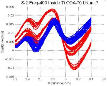
78 (a) (b) (c) (d) 66

79 (e) Figure 53 Collection of All Line Scans for Defect-free and Defective Fasteners Note: Outside Row (Left) and Inside Row (Right): (a) single line (central), (b) 3 lines, (c) 5 lines, (d) 7 lines and (e) 11 lines 67

80 (a) (b) (c) (d) 68

81 (e) Figure 54 Scatter Plot of Features for Multiple Lines Note: Outside Row (Left) and Inside Row (Right): (a) single line (central), (b) 3 lines, (c) 5 lines, (d) 7 lines and (e) 11 lines The SNR values for single and multiple line plots are shown in Table 9. The SNR values obtained using amplitude based features are also included for comparison. S-2 (Ti, 0.16 inch, 400 Hz) Skin Fastener Thickness Row Table 9 SNR Values for Different Methods 0.16 Outside 3(eddy current) 1.5(eddy current) 0.16 Inside 2.5(eddy current) Signal-to-Noise (X:1) (eddy current) 1.5(eddy current) 45.0(Mag) 18.0(Mag) 14.0(Mag) 9.6(Mag) 316.7(Single) 49.8(Single) 16.4(Single) 17.1(Single) 455.9(3 lines) 74.3(3 lines) 23.6(3 lines) 27.3(3 lines) 355.5(5 lines) 56.5(5 lines) 18.7(5 lines) 22.3(5 lines) 290.9(7 lines) 46.4(7 lines) 15.8(7 lines) 18.7(7 lines) 78.2 (11 lines) 13.1 (11 lines) 4.8 (11 lines) 5.6 (11 lines) 1.5(eddy current) 1 (eddy current) 1 (eddy current) 20.6(Mag) 8.2(Mag) 4.4(Mag) 4.0(Mag) 292.1(Single) 64.5(Single) 17.1(Single) 18.2(Single) 252.5(3 lines) 54.5(3 lines) 15.2(3 lines) 15.8(3 lines) 189.9(5 lines) 41.7(5 lines) 11.8(5 lines) 12.2(5 lines) 112.9(7 lines) 25.5(7 lines) 7.5(7 lines) 7.8(7 lines) 43.8 (11 lines) 10.8 (11 lines) 3.4 (11 lines) 3.5 (11 lines) 69

82 4.2 OPTIMIZATION OF PARAMETERS THROUGH MODELING Model validation The finite element model developed for MR inspection of multilayer test samples was first validated using experimental measurements from both the calibration sample with notch and a S-2 standard sample. The validation results are presented in this section Model validation using notch calibration standard sample. The calibration sample is made of standard aluminum. The sample is a plate of dimensions 16 inches X 10 inches and of thickness inch. A notch of dimensions 0.05 inch width and 0.25 inch depth is machined at the center of the sample. A photograph of the sample is shown in Figure 55. (a) Figure 55 Photographs of (a) the Sensor Head at the Zero-Balancing Calibration Position and (b) an Overhead View of the Calibration Sample with Slot Down the Middle. The Sensors and Excitation Current are Aligned Parallel to the Slot. The three-dimensional domain of the FE model and the corresponding mesh are shown in Figure 56 and Figure 57, respectively. (b) 70

83 Figure 56 Sample Geometry Used in the Model (a) Figure 57 (a) SidView and (b)top View of the Finite Element Mesh The FEM solutions produce the electric scalar potential V and magnetic vector potential A at each node in the solution region. The magnetic flux density B = X A is computed and its normal component, is compared with the measured MR signal. Figure 58 shows threedimensional plot of the real and imaginary part of the model computed magnetic flux density. The two-dimensional scan across the slotted sample is applied to obtain the sensor signal. Figure 59 shows geometry of the scan. (b) 71

84 (a) Figure 58 Modeling Results of the Normal Component of the Magnetic Flux Density (a) Real Part (b) Imaginary Part (b) Figure 59 Geometry of Scan Plan Experimental signals for the sample were available for various demodulation angles as described in section The in-phase and quadrature components were demodulated to generate a mixed signal using varying demodulation angle δ. The mathematical form for the calibrated demodulated signal for sensor n at arbitrary detection angle δ is: n δ δ n n n n n 0 π n π 2 S S = α ( S S S S )cos( δ ) + α ( S S S S )sin( ) (43) A0 An where S 0 Sn = cos( φ δ ) δ n. 2 In finite element modeling, the zero balancing term 0 S and the scaling factor α n are 0 and 1, respectively since these two terms are only useful in experimental data analysis. 0 Sn δ 72

85 Since the initial phase of excitation current in the FE models is different from what is " " π used in experiments, the detection phase δ is calibrated to δ, where δ = δ. A 4 comparison of model and experimental signals are shown in Figure 60, where the calibrated " detection phase δ spans half a cycle from 0 to 180 degrees in steps of 30 degrees. We can conclude that the model result accurately predicts the experimental measurements. 73

86 (a) model prediction (b) experimental signal Figure 60 Comparison of Demodulated and Calibrated Signal Across the Calibration Slot Model validation using S-2 Standard Sample A schematic of the geometry of S-2 standard sample with H section crack, sensor configuration and scan direction are shown in Figure

87 Figure 61 Geometry for S-2 Sample. The fastener material in this sample is Titanium. The side view shows top layer truncated in accordance with the S-2 sample geometry. The model also simulates the gap between the two top skins of S-2 sample. The current is parallel to the notch length and the scan direction is perpendicular to it. The H section crack is not applied in the FEM so that the comparison is between simulated and experimental signals for the crack free rivet. The optimized threedimensional FE mesh for this sample with edge is shown in Figure

88 (a) (b) Figure 62 FE Mesh for S-2 Sample: (a) Side View (b) Top View The modeling results at 400 Hz excitation frequency are shown in Figure 63. The real and imaginary of the normal component of magnetic flux density are shown in Figure 63(a) and (b). The magnitude of the magnetic flux density is presented in Figure 63(c). 76

89 (a) (b) (c) Figure 63 Magnetic Flux Density for S-2 Sample Geometry in Figure 62 at 400 Hz (a) Magnitude (b) Real Component (c) Imaginary Component The corresponding experimental data from the rivet is shown in Figure

90 Figure 64 MRS Data for Crack-free Fastener in S-2 Sample at 400 Hz Note: The line scan is marked by the red dashed line. A comparison between simulation and experimental results is presented. Line scans in the x-direction across the center of the fastener is extracted from the real and imaginary image data (both the simulation and experiment) which are then mixed using different demodulation or detection angles. The detection angle α and the mixed MR sensors signal is given by S = S cos( α) + S sin( ), (44) α where S α, S 0 and 0 π α 2 S π are the mixed, in-phase and quadrature signals, respectively. 2 The mixed model and experiment signals are compared for a number of detection angle values in Figure 65 through Figure 67. The detection angle for experimental signals is changed from 80 to 110 degrees, 120 to 150 degrees and 160 to 190 degrees in the three figures, respectively. Both the magnitude and shape of the signals are remarkably similar. These validation results for the model allow the use of the model in conducting the series of simulations for the parametric study described in the following sections. 78

91 Figure 65 Comparison between Experimental and Modeling Signal with Various Detection Phases. 79

92 Figure 66 Comparison between Experimental and Modeling Signal with Various Detection Phases 80

93 Figure 67 Comparison between Experimental and Modeling Signal with Various Detection Phases Parametric Studies Introduction Once the FEMs were validated, then studies of parameters could be pursued to assess optimum scanning conditions for MR sensors. Table 10 lists parameters of interest that could be evaluated within the program constraints. The table contains the range of the parameters that would be examined in the modeling studies. 81

94 Parameter Table 10 Parameter Study Table Range of Value Tested Frequency (khz) 0.1, 0.2, 0.4, 0.5, 0.7, 1.0, 2.0, 3.0, 5.0, 7.0 Sensor liftoff (inch) , , 0.015, 0.1, 0.15, 0.2 Conductivity of top layer (%IACS) Conductivity of bottom layer (%IACS) Conductivity of fastener (%IACS) Between 28 and 33 Between 30 and 36 Titanium (6Al, 4V): 1.0, 2.2, 3.1 Fastener to edge distance (inch0 0.40, 0.50, 0.60, 0.70, 0.80 Crack dimensions (inch) 0.20, 0.22, 0.25, Frequency Effect The parameter that has a significant impact on the measured MR signal is the excitation frequency. Since most aircraft geometry contains multiple layers with cracks in second and third layer the operating frequencies is largely at the low end. The range of frequencies considered in this study are: 0.1, 0.2, 0.4, 0.5, 0.7, 1.0, 2.0, 3.0, 5.0, and 7.0 khz. The geometry of the S2 sample and sensor configuration and finite element mesh are shown in Figure 61 and Figure 62. A 0.3 inch second layer defect is introduced under the fastener through the second layer on the side of the stringer edge. The normal component of magnetic flux density Bz is calculated for each frequency, for both, the crack free case and 0.3-inch crack case. Figure 68 shows the simulation results at a frequency of 0.1 khz. The images in 3(a), 3(c) and 3(e) are the magnitude, real and imaginary parts of the normal component of flux density for crack free case at a liftoff of inch. Images in 3(b), 3(d) and 3(f) are the corresponding magnitude, real and imaginary parts of the normal component of flux density for 0.3-inch crack geometry. Figure 69 through Figure 73 present similar model predicted results for frequencies of 400, 500, 700, 2000, and 7000 Hz. The real imaginary and absolute magnitude of the normal component magnetic flux density for both defect free and 0.3-inch crack are presented. 82

95 (a) (b) (c) (d) (e) Figure 68 Simulation Results for 100 Hz Frequency (f) 83

96 (a) (b) (e) (d) (e) Figure 69 Simulation Results for 400 Hz Frequency (f) 84

97 (a) (b) (c) (d) (e) Figure 70 Simulation Results for 0.5 khz Frequency (f) 85

98 (a) (b) (c) (d) (e) Figure 71 Simulation Results for 0.7 khz Frequency (f) 86

99 (a) (b) (c) (d) (e) Figure 72 Simulation Results for 2.0 khz Frequency. (f) 87

100 (a) (b) (c) (d) (e) SKEWNESS CALCULATIONS Figure 73 Simulation Results for 7.0 khz Frequency Although the defect indication is visible in most of the images, a simple method for determining the optimum value of frequency is presented in this section via a quantitative measure of the asymmetry in the two lobes of the image. A simple skewness function for quantifying the asymmetry is calculated based on the peak values of the two lobes of the fastener image, and is defined in Equation (45). (f) 88

101 max{ B1, B2 } S 1 =. (45) min{ B, B } 1 2 The parameters of this function are shown pictorially in Figure 74. The value of S 1 is calculated for the fastener image obtained at each frequency and is plotted in Figure 75. Figure 74 Surface Plot of the Image Data Showing the Asymmetry in Two Lobes of Fastener Image Skewness vs. Frequency Skewness S Frequency(kHz) Figure 75 Skewness Versus. Frequency for Results with 0.3-inch crack. From Figure 75 it is seen that at lower frequencies the skewness values are much higher than 1 and the crack is easily detected. At higher frequency, the crack is hard to see due to the skin depth effect. The skewness plots show that the optimal operating frequency is 0.4 khz. Further, the modeling results indicate that as the frequency increases, the images are sharper and the edge effect vanishes, but the crack detection ability decreases because of the skin depth effect. 89

102 SNR CALCULATIONS An alternate method for optimizing frequency of operation is to select a frequency that maximizes the POD or equivalently the SNR of the signal. In this study, SNR values are calculated with simulation results obtained at frequencies: 100 Hz, 400 Hz, 500 Hz, 700 Hz and 1000 Hz. Both crack-free fastener and the case of a fastener with 0.3 inch subsurface crack were simulated. The fastener image at each frequency is analyzed using the procedure described in section The image data was preprocessed using the optimum detection angle at each frequency and the line scans across the center of the fastener was extracted. The same features developed in section using experimental data from S-2 sample are applied for simulated signal. The features are as shown in Equations (45) and (47), which are the same as ( ) and ( ). F MAE = 1 N N L [ i] 1 M D i= 1 M j= 1 L ND _ j[ i] (46) F MSE = 1 N N ( L [ i] 1 M D i= 1 M j= 1 L i 2 ND _ j[ ]) (47) F MAE is the feature calculated from mean absolute error and the F MSE is calculated from mean square error. In Equations 46 and 47, N is the length of the mixed 1-D data vector, M is the total number of non-defective rivets. L D [i] is the ith pixel of mixed data for different frequencies and L ND_j [i] is set to zero vector as the baseline signal. The line scans at different frequencies for the 0.3 inch subsurface crack signals are shown in Figure

103 Figure 76 Simulated Line Scans at Different Frequencies for 0.3-inch Subsurface Cracks after ODA Processing The SNR definition used earlier is modified. The definition used in analyzing experimental data is provided in Equation (48). The modified equation for analysis of simulated data is given in (49), where the mean and variance are set to 0 and 1, respectively, SNR M = M i= 1 ( F i m 2 0 i ) σ 2 0i (48) M 2 SNR M = F i. (49) i= 1 where M = 2 in this case. A scatter plot of two-dimensional feature vector in the feature space is shown in Figure 77. A classification rule can be devised based on partitioning the defect free fastener (green dot) from the feature vector corresponding to the 0.3 inch crack data (red triangle). The SNR value is proportional to Euclidean distance between (0,0) and the feature at each frequency. The SNR versus frequency plots are shown in Figure 78 and it is seen that the SNR maximum is at 400 Hz frequency. 91

104 Figure 77 Two-Dimensional Feature Space for Simulated Data at Different Frequencies Figure 78 SNR versus Frequency for Simulated Signal for S-2 Sample with 0.3 inch Subsurface Crack From Figure 77, the model predicted optimum frequency is 400 Hz, which is close to the optimum frequency of 450 Hz obtained from the experimental signals for S-2 sample Sensor Liftoff Effect The parametric effect of sensor liftoff on the signals was studied. Liftoff values considered were , , , 0.1, 0.15, and 0.2 inches. The geometry and finite 92

105 element mesh of the S2 sample and sensor configuration are shown in Figure 61 and Figure 62. A 0.3-inch second layer defect is introduced under the fastener. The normal component of magnetic flux density Bz is calculated at excitation frequency of 400 Hz. The real, imaginary and magnitude of the normal component of magnetic flux density images are plotted for each individual liftoff value in Figure 79 through Figure 84. (a) (b) (c) Figure 79 Bz Plots for inch Liftoff (a) Real, (b) Imaginary, (c) Magnitude (a) (b) (c) Figure 80 Bz Plots for inch Liftoff (a) Real, (b) Imaginary, (c) Magnitude (a) (b) (c) Figure 81 Bz Plots for inch Liftoff (a) Real, (b) Imaginary, (c) Magnitude 93

106 (a) (b) (c) Figure 82 Bz Plots for 0.1-inch Liftoff (a) Real, (b) Imaginary, (c) Magnitude (a) (b) (c) Figure 83 Bz Plots for 0.15-inch Liftoff (a) Real, (b) Imaginary, (c) Magnitude (a) (b) (c) Figure 84 Bz Plots for 0.2-inch Liftoff (a) Real, (b) Imaginary, (c) Magnitude To see the variation in the signals with sensor liftoff, the peak to peak values in line scans across the center of the fastener are considered. The real and imaginary parts of the line scans are plotted in Figure 85 (Real) and Figure 86 (Imaginary). The real and imaginary data are demodulated using the optimum detection angle of 70 degrees at 400 Hz and the resulting mixed signals are shown in Figure 87. The peak to peak values of Bz (real, imaginary, magnitude and mixed) at each liftoff are listed in Table 11 and plotted in Figure

107 2 x 10-8 Sensor Liftoff Real Line Plot " " 0.015" 0.053" 0.1" 0.15" 0.2" x 10-4 Figure 85 Line Scans across the Center of Fastener of Real Part 8 x 10-9 Sensor Liftoff Imaginary Line Plot " " 0.015" 0.053" 0.1" 0.15" 0.2" x 10-4 Figure 86 Line Scans across the Center of Fastener of Imaginary Part 95

108 3 x 10-9 Sensor Liftoff Mixed Line Plot using ODA " " 0.015" 0.053" " 0.15" 0.2" Figure 87 Mixed Line Scans Using ODA x 10-4 Table 11 Peak-to-Peak Values of Bz for Various Sensor Liftoffs Sensor liftoff (inch) Real Imaginary Mixed e e e e e e e e e e e e e e e e e e e e e

109 Figure 88 Peak Values of Real, Imaginary, and Mixed MR Signals Versus Liftoff As expected, when the sensor liftoff increases, the measured signal decreases. Since the optimum detection angle is selected based on minimum peak-to-peak value in the image data of the fastener, it is seen that in the mixed signals the overall spread in the peak value with liftoff is also lower; hence, the change in signal values with liftoff is relatively flatter than that of raw data reported Conductivity of Top Layer Effect The conductivity values for the top layer were selected according to the Parametric Table presented earlier. The operation frequency is chosen as 400 Hz and liftoff is chosen as inch. The geometry of the S-2 standard including a fastener with 0.3 inch defect on the bottom layer is modeled. The nominal conductivity for top layer plate for S-2 sample is 29.6 percent IACS, and the range of conductivity of the top layer plate is assigned values from 28 percent to 33 percent IACS. Figure 89 through Figure 94 present simulation results of real, imaginary, and magnitude value of the normal component of magnetic flux density for different values of top layer conductivity. Table 12 shows the peak value of the signal magnitude at different values of conductivity. 97

110 (a) (b) (c) Figure 89 Bz with 28% Iacs Top Layer Conductivity (a) Real, (b) Imaginary, (c) Magnitude (a) (b) (c) Figure 90 Bz with 29% Iacs Top Layer Conductivity (a) Real, (b) Imaginary, (c) Magnitude (a) (b) (c) Figure 91 Bz with 30% Iacs Top Layer Conductivity (a) Real, (b) Imaginary, (c) Magnitude 98

111 (a) (b) (c) Figure 92 Bz with 31% Iacs Top Layer Conductivity (a) Real, (b) Imaginary, (c) Magnitude (a) (b) (c) Figure 93 Bz with 32% Iacs Top Layer Conductivity (a) Real, (b) Imaginary, (c) Magnitude (a) (b) (c) Figure 94 Bz with 33% Iacs Top Layer Conductivity (a) Real, (b) Imaginary, (c) Magnitude 99

112 Table 12 Peak Values of Magnitude of Bz for Various Top Layer Conductivities Conductivity (% IACS) Conductivity (Siemens/m) Peak value of the signal magnitude (Tesla) e e e e e e e e e e e e-8(1.4% difference vs. 28% IACS) Figure 95 shows a plot of peak value of magnitude signal magnitude versus top layer plate conductivity. Figure 95 Peak Value of the Signal Magnitude Versus Top Layer Plate Conductivity From the results in Table 12 and the Figure 95, it is seen that the peak value of the signal increases slightly when top layer plate conductivity increases. This is as expected since increase in the top layer plate conductivity increases the induced eddy currents thereby increasing the amplitude of the measured signal. 100

113 Conductivity of Bottom Layer Effect The conductivity values for the bottom layer were selected according to the Parametric Table presented earlier. For bottom layer plate, the conductivity value ranges from 30 percent IACS to 36 percent IACS. The operation frequency is chosen as 400 Hz and liftoff is chosen as inch. The geometry of the S-2 standard including a fastener with 0.3 inch defect on the bottom layer is modeled. The nominal conductivity for bottom layer in the S-2 standard is 33.5% IACS, and the range of the bottom layer conductivity is chosen to vary from 30% IACS to 36% IACS. Figure 96 through Figure 102 present simulation results of real, imaginary, and magnitude value of the normal component of magnetic flux density for different values of bottom layer conductivity. Table 13 shows the peak value of the signal magnitude at different values of conductivity. Figure 103 shows the plot of peak value of the signal magnitude versus bottom layer plate conductivity. (a) (b) (c) Figure 96 Bz with 30% Iacs Bottom Layer Conductivity (a) Real, (b) Imaginary, (c) Magnitude (a) (b) (c) Figure 97 Bz with 31% Iacs Bottom Layer Conductivity (a) Real, (b) Imaginary, (c) Magnitude 101

114 (a) (b) (c) Figure 98 Bz with 32% Iacs Bottom Layer Conductivity (a) Real, (b) Imaginary, (c) Magnitude (a) (b) (c) Figure 99 Bz with 33% Iacs Bottom Layer Conductivity (a) Real, (b) Imaginary, (c) Magnitude (a) (b) (c) Figure 100 Bz with 34% Iacs Bottom Layer Conductivity (a) Real, (b) Imaginary, (c) Magnitude 102

115 (a) (b) (c) Figure 101 Bz with 35% Iacs Bottom Layer Conductivity (a) Real, (b) Imaginary, (c) Magnitude (a) (b) (c) Figure 102 Bz with 36% Iacs Bottom Layer Conductivity (a) Real, (b) Imaginary, (c) Magnitude Table 13 Peak Values of Bz Magnitude for Various Bottom Layer Conductivities Conductivity (% IACS) Conductivity (Siemens/m) Peak value of the signal magnitude (Tesla) e e e e e e e e e e e e e e-8 (2.5% difference versus 30% IACS) 103

116 Figure 103 Peak Value of the Signal Magnitude Versus Bottom Layer Plate Conductivity From the results presented above, it is seen that the peak value of the signal decreases when bottom layer conductivity increases. When the bottom layer plate conductivity increases, the induced eddy current becomes more concentrated around the bottom surface and the observed signal on the top surface is reduced Conductivity of Fastener Effect The conductivity of fastener was varied as described in the parameter table. The geometry of the S2 sample with a 0.3 inch crack and finite element mesh are as shown in Figure 56 and Figure 57. The operation frequency is chosen as 400 Hz and liftoff is chosen as inch. The different conductivity values for the fastener were chosen to be 1.0 percent IACS, 2.2 percent IACS, and 3.1 percent IACS. The real, imaginary, and magnitude values of magnetic flux density at the MR sensor for different conductivity values are plotted in Figure

117 Figure 104 Real, Imaginary, and Magnitude of Magnetic Flux Density for Conductivity Values of Ti Fastener (1.0 percent Iacs, 2.2 percent Iacs, and 3.1 percent Iacs) as Indicated on the Left The variation of the peak values are summarized in Table 14. The fastener conductivities considered in this study does not affect the signals with any significance. Table 14 Effect of Fastener Conductivity on Peak Value of Magnitude Signal Fastener Conductivity Peak values e e e-008 of magnitude Fastener to Edge Effect A commonly encountered problem in airframe geometry is the influence of surface and subsurface edge on fastener and crack signals. The edge discontinuity behaves as a large defect and generates its own signature that can affect the defect signal and thereby lead to misinterpretation of MR data. This section describes a systematic study of the effect of fastener-to-edge distance on the defect signal. The S-2 sample fastener with a 0.3 inch, second layer crack geometry presented in section is considered. The edge is in the 105

118 second layer and the nominal fastener-to-edge distance for S-2 sample is 0.6 inch. The range of values for parametric variations is 0.4 to 0.8 inch. Simulations were performed at 400 Hz excitation frequency and inch liftoff. The normal component of the magnetic flux density Bz is calculated at the prescribed liftoff and the resulting image data are plotted for each simulation. The real, imaginary, magnitude and demodulated images are presented. The demodulated image is derived using optimum detection angle (ODA) which is 70 degrees. Figure 105 to Figure 109 show the real, imaginary, magnitude and demodulated images for varying fastener-to-edge distance in the range 0.4 to 0.8 inch. Real Imaginary Magnitude Demodulated Figure 105 Real, Imaginary, Magnitude, Demodulated Bz for Fastener Edge Distance = 0.4 inch 106

119 Real Imaginary Magnitude Demodulated Figure 106 Real, Imaginary, Magnitude, Demodulated Bz for Fastener Edge Distance = 0.5 inch Real Imaginary Magnitude Demodulated Figure 107 Real, Imaginary, Magnitude, Demodulated Bz for Fastener Edge Distance = 0.6 inch 107

120 Real Imaginary Magnitude Demodulated Figure 108 Real, Imaginary, Magnitude, Demodulated Bz for Fastener Edge Distance = 0.7 inch Real Imaginary Magnitude Demodulated Figure 109 Real, Imaginary, Magnitude, Demodulated Bz for Fastener Edge Distance = 0.8 inch The line plots are extracted from all the image data and plotted. Figure 110 and Figure 111 show the line scans across the center of the rivet image of real and imaginary parts. Figure 112, shows the line scan of the demodulated signal using ODA. When the fastener-toedge distance increases, the edge effect on the right side of the fastener is decreased, so the magnitude of the signal on the right lobe will decrease slightly. 108

121 1.5 x 10-8 Parameter-Fastener-edge-dist (Real,bottom 0.3" crack) Signal(T) inch 0.5 inch 0.6 inch 0.7 inch 0.8 inch X Distance(m) Figure 110 Line Scans Across the Center of the Fastener for Real Part of Bz x 10-8 Parameter-Fastener-edge-dist (Imag,bottom 0.3" crack) 0.4 inch 0.5 inch 0.6 inch 0.7 inch 0.8 inch 0 Signal(T) X Distance(m) Figure 111 Line Scans Across the Center of the Fastener for Imaginary Part of B 109

122 1.5 x Parameter-Fastener-edge-dist (ODA,bottom 0.3" crack) 0.4 inch 0.5 inch 0.6 inch 0.7 inch 0.8 inch Signal(T) X Distance(m) Figure 112 Line Scans Across the Center of the Fastener for Mixed Signal Using ODA To further examine the effect of edge on defect signal amplitude, the signal from a defective fastener for the largest fastener-to-edge distance is calculated and subtracted from the defect signal, in each case, at the defect location. Assuming that there is minimal effect on defect signal when the edge is the farthest, this value reflects the effect of an edge in the proximity of the fastener. The defect signal amplitude calculated in this manner is summarized in Table 15 and plotted in Figure 113. Figure 113 Edge Effect on Defect Signal Amplitude: Real, Imaginary, and Mixed Signals Versus Fastener-to-Edge Distance 110

123 Table 15 The Peak-to-Peak Values Versus Fastener-to-Edge Distance Fastener-edge Distance (inch) Real signal e e e e-7 0 Imag signal e e e e-6 0 Mixed signal e e e e-6 0 From Figure 113, it is observed that the closer the fastener is to an edge the more effect on defect signal. The signal due to the edge adds to the defect signal which increases with proximity of fastener to the edge Crack Dimension Effect Based on the S-2 flaw schematics diagram, four different trapezoidal crack dimensions were modeled including the case of a crack-free fastener. The radial dimensions of the top of crack top were chosen to be 0.2, 0.22, 0.25 and 0.3 inch. The crack geometry was tapered towards the bottom surface. The sensor liftoff was kept at inch and the frequency was chosen to be 500 Hz. The normal component of the magnetic flux density (Bz) is calculated and plotted. The real, imaginary, and magnitude of the complex flux density are plotted in Figure 114 through Figure 118. (a) (b) (c) Figure 114 Bz for 0.2 inch Crack (a) Real, (b) Imaginary, (c) Magnitude 111

124 (a) (b) (c) Figure 115 Bz for 0.22 inch Crack (a) Real, (b) Imaginary, (c) Magnitude (a) (b) (c) Figure 116 Bz for 0.25 inch Crack (a) Real, (b) Imaginary, (c) Magnitude (a) (b) (c) Figure 117 Bz for 0.3 inch Crack (a) Real, (b) Imaginary, (c) Magnitude 112

125 (a) (b) (c) Figure 118 Bz for no Crack (a) Real, (b) Imaginary, (c) Magnitude In order to see the variation in the signals with increasing crack dimensions, the line scans across the center of the fastener image data are plotted. The real part of the magnetic flux density is shown in Figure 119 and Figure 120 is the image of the imaginary part. The demodulated signal using an optimum detection angle of 70 degree at 500 Hz is shown in Figure x 10-8 Real Line Plot No Defect.2" defect.22" defect.25" defect.3" defect x 10-4 Figure 119 Line Scans across the Center of the Fastener for Real Image Data 113

126 8 x 10-9 Imaginary Line Plot 6 4 No Defect.2" defect.22" defect.25" defect.3" defect x 10-4 Figure 120 Line Scans Across the Center of the Fastener For Imaginary Image Data 114

127 3 x 10-9 Mixed Line Plot using ODA No Defect.2" defect.22" defect.25" defect.3" defect Figure 121 Mixed Line Scans Using ODA of 70 Degrees The defect signal amplitude is calculated using the peak-to-peak value of all 3 signals, real, imaginary, and mixed. The values calculated are listed in Table 16 and plotted in Figure 122. The defect signal values are also recalculated after subtracting the value obtained for the crack-free fastener. These values are summarized in and plotted in Figure 123. x 10-4 Table 16 The Peak-to-Peak Values of Bz for Various Crack Dimensions Crack width on top (inch) Real Imaginary Mixed e e e e e e e e e e e e e e e

128 4 x Peak-to-peak Values vs. Crack Dimension Real Imaginary Mixed (ODA = 70) 2 Signal (T) Crack Area (square inch) Figure 122 Peak-to-peak values of Real, Imaginary, and Mixed MR Signals Versus Crack Area Table 17 The Peak-to-Peak Values of Bz for Various Crack Dimensions (after Subtracting the Value Obtained for the Crack-Free Fastener) Crack width on top (inch) Real Imaginary Mixed e e e e e e e e e e e e

129 Peak to Peak Value vs Crack Dimension 3.25E E-08 Peak To Peak Value of Bz (Tesla) 2.25E E E E-09 Real Imaginary Mixed 2.50E E Crack Dimension Figure 123 Peak-to-Peak Values of Real, Imaginary, and Mixed MR Signals Versus Crack Area 4.3 OPTIMIZED SCANNING The first set of scans of the S-2 sample, shown through Sections and , were made as a benchmark from which the modeling calculations could be validated, as was shown in Section The frequency parametric study, shown in Section , indicated at one point that the frequency ought to be increased beyond the maximum 500 Hz used in this first set of scans. Indeed, as indicated in the above description of these scans and shown in Figs through , the differentiation between fasteners with and without cracks appears better with higher frequencies, but a visual inspection of the various c-scans did not easily yield a quantitative justification of that statement. This modeling result of higher frequency prompted a new set of scans to be made. All four of the test standards: S-1, S-2, S-3 and S-4, were rescanned over the same frequency range as before, f = 100 to 500 Hz at steps of 50 Hz. Beyond this, the S-2 standard was scanned from 550 to 800 Hz in steps of 50 Hz. In addition, each of the scans was made five times. This was done in support of the advanced feature recognition algorithm development to provide multiple sets of data for statistical analysis Performance on New data from S2 sample The second dataset provided by Boeing includes data at 15 frequencies from 100 Hz to 800 Hz in steps of 50 Hz. For each frequency, the MR data was acquired five times using five independent scans. For instance, the Ti fastener images of S-2 sample at 400 Hz and 650 Hz for five scans are shown in Figure 124 and Figure 125 with optimum detection angles of

130 and 80 degrees, respectively. As we can see, the outcomes of five different scans are almost identical to each other in two-dimensional images. (a) (b) (c) (d) (e) Figure 124 Titanium Fastener Images for S-2 Test Standard at 400 Hz with ODA =70 degrees in Five Experimental Scans (a) to (e) 118

131 (a) (b) (c) (d) (e) Figure 125 Titanium Fastener Images for S-2 Test Standard at 650 Hz with ODA = 80 degrees in Five Experimental Scans (a) to (e) The data acquired on the S-2 standard sample with Titanium fasteners at different frequencies was analyzed. Figure 126 and Figure 127 present the results in the form of line plots and scatter plots in feature space, respectively. 119

132 (a) (b) (c) 120

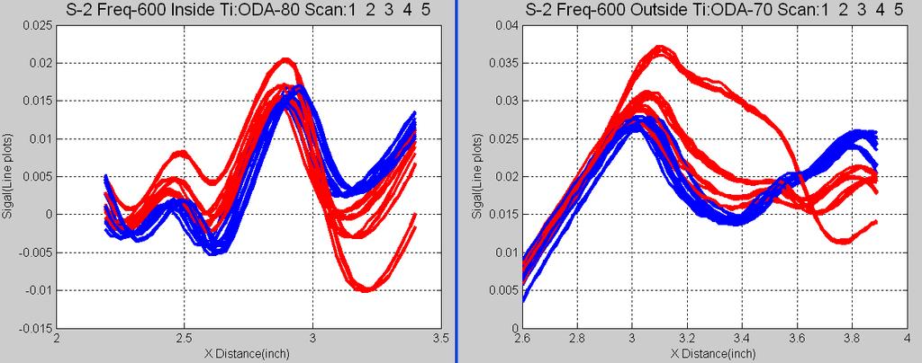
133 (d) (e) (f) 121

134 (g) (h) Figure 126 Collection of all Line Scans for Defect-Free (blue) and Defective (red) Fasteners Note: Outside row (right) and inside row (left): (a) to (h) for frequencies 100 Hz to 800 Hz in steps of 100 Hz 122

135 (a) (b) (c) 123

136 (d) (e) (f) 124

137 (g) Note: (h) Figure 127 Scatter Plot of Features-Defect-Free (green), Defective (red) Outside row (right) and Inside row (left): (a) to (h) represent frequencies 100 Hz to 800 Hz in steps of 100 Hz The SNR values calculated for the S-2 sample data from inspection of both, outside and inside fasteners, at various frequencies are summarized in Table 18 and Table

138 Table 18 SNR Values for S-2 Sample - Outside Fasteners at Different Frequencies OUTSIDE Frequency(Hz) 0.20 inch 0.22 inch 0.25 inch 0.30 inch

139 Table 19 SNR Values for S-2 Sample - Inside Fasteners at Various Frequencies INSIDE Frequency(Hz) 0.20 inch 0.22 inch 0.25 inch 0.30 inch

140 Figure 128 Scatter Plot of Features Defect-Free (green), Defective (red) Note: Outside row (right) and Inside row (left) at the optimum frequencies: 450 Hz and 550 Hz, respectively From the analysis results of experimental data at different frequencies, one can generate a plot of SNR versus frequency as presented in Figure 129 and Figure 130, for outside and inside fasteners. These results show that the optimum frequency that maximizes the SNR criteria is 450 Hz for outside fasteners and that for inside fasteners is 550 Hz. Figure 129 SNR (Raw and Curve-Fitted) Plots Versus Frequency for S-2 Outside Fasteners 128

141 Figure 130 SNR (Raw and Curve-Fitted) Plots Versus Frequency for S-2 Inside Fasteners Optimized Scan Conclusions As was mentioned in the previous section, a full, comprehensive set of scans was made of the S-2 test standard that spanned frequencies from 100 to 800 Hz. This span was larger than the original set, shown in Section Based on earlier work it was suggested that optimum frequency would be found higher than the 500 Hz that was scanned at that time. Subjectively, it was determined that Hz was the best scan frequency range, but that was based more upon the visual interpretation of the c-scans rather than any quantitative determination. It was shown in Figure 129 and 130 that this new set was indeed optimized close to that range, now based upon contour features quantitatively determined through equations rather than the subjective look of scan plots. Both the modeling with frequency parameter and the application of advanced feature recognition algorithms agree with the more anecdotal conclusion of this best frequency range. 4.4 TRANSITION TO MAUS As was mentioned briefly in Section , an MR Sensor module is currently being added to the MAUS system in Boeing St. Louis. The findings of this study have been made available to that program, and in particular the feature recognition algorithms presented throughout Section will be taken into consideration for incorporating automatic feature detection with the MAUS system. 129

142 As this new field deployable system comes online, there are interesting and pertinent findings and conclusions that have been reported. One of the more impactful insights to this kind of modeling and laboratory testing effort involves the comparison between fabricated test standards and actual airframe structures that are being scanned. As was shown in Figure 18, the MR/MAUS system has been used to scan an actual wing. There are two points to note: First, the arrangement of steel and titanium fasteners, such as seen in the S-2 test standard that was so prominently studied in this program, is not a realistic example of what is actually encountered in the field on real structures. Rather, there is typically a non-ordered collection of many kinds of fasteners, particularly on older aircraft. This fact may itself not be of any immediate concern when making more fundamental developments on standards such as the S- 2; however, it is important to note that the different materials are not usually so isolated. Second, on typical airframe structures such as the wings that have been scanned using the MR/MAUS system, there is no bottom layer edge encountered that is so close to the fasteners that it causes the kind of interference seen in the test measurements and considered in the modeling work. The absence of such an edge is welcome, of course, in that it tends to overwhelm the smaller MR sensor response from cracks parallel to and near the edge. The report from the MR/MAUS effort is that the kind of bottom layer geometry that comprises the S-2 test standard is simply not a realistic representation of the kind of structures being encountered in the field. This implies that the test standard arrangements themselves may be driving unnecessary efforts in discerning cracks near edges when this situation may indeed not be common, at least in the MR/MAUS scans presently under consideration. 130

143 5. CONCLUSIONS AND RECOMMENDATIONS The results and findings of Advanced Nondestructive Evaluation Sensor Modeling for Multi-Site Inspection have been presented. A FEM scheme was developed to accurately represent the fields and response of MR sensors from AC currents induced in complex metal geometries that are of interest to the Air Force, namely, cracks of various shapes and sizes in the vicinity of fasteners that splice metal layers together as on an airframe. This model was developed in calibration with measurements made in a laboratory environment. Once satisfactorily calibrated, the model was used to conduct a variety of parametric studies including frequency, sensor liftoff, conductivity of layers, fastener to edge distance and crack dimension. In addition to the modeling efforts presented, the results of meticulous analysis of the laboratory measurements were presented as part of the development of automated feature recognition. The data was further processed to reduce the results to figures of merit, various feature values that incorporated both magnitude and shape of signal and ultimately SNRs. It has been noted that applying meaningful quantitative conclusions to c-scan results through subjective observation is challenging and not necessarily repeatable, particularly in borderline cases of deep and/or small cracks. These automated algorithms have served to place an objective value to cracks as they appear in MR sensor data. As a result of quantitative data reduction it has been possible to establish a signal to noise ratio value for the MR sensing. With this evaluation it was possible to show that MR sensors offer considerable value over conventional eddy current inspections with the possibility of improvements in sensitivity by over an order of magnitude. The results of this study lead to the following recommendations: 1. MR Sensor Implementation The improved detection capability of MR sensors measured in this program indicated that implementation under the MR MAUS program is well justified. However, additional operational schemes should also be considered to obtain the potential value of this inspection method. 2. Reverse Modeling This program has consisted primarily of forward modeling, in which a known geometry, arrangement of cracks, etc. is modeled in order to obtain sensor response to some parametric variation such as frequency. A more challenging, yet more rewarding effort would be to follow with reverse modeling that would ultimately take the results and backward model into the more likely scenario that is being encountered. For example, given a result, what are the most likely size and direction of the underlying crack? 3. Expanded Parametric Studies There are additional parametric studies that need be conducted, partly from the list generated through this program, but more importantly through feedback from the MR/MAUS program or in response to current Air Force concerns. 4. Advanced MR Sensor Development This work has utilized straightforward AC, timeindependent excitation signals. There is interest in examining pulsed MR Sensor scanning in which time response is incorporated into the scan. 131

144 5. Sensor Orientation This work has concentrated on MR sensing using B z measurements with the available orientation of the MR devices. The modeling results indicate that B x and B y may contain additional information to discriminate important characteristics and should be investigate. 132

145 6. REFERENCES 1 Aging of U.S. Air Force Aircraft, National Research Council Final Report, Publication NMAB-488-2, National Academy Press, Washington, D.C., The Air Force in Facts and Figures, Air Force Magazine, May Rempt, R., Magnetoresistive Sensors for Eddy Current Imaging NDE, AFRL-ML-WP- TR-2003, Final report for Feb. 15, 2002 through July 31, Rempt, R. and Koltenbah, B., Multi-layer Cracks and Multi-Site Damage NDE, AFRL- ML-WP-TR-2006, Final Report for July 2003 through October Palmer, D. and Wood, N., Magnetoresistive Sensor Technology for MAUS Aircraft Inspection, Contract F D-5204, Delivery Order 0025, subcontract 06-S C1, 07 July March Dodd, C.V. and W.E. Deeds, Analytical Solutions to Eddy-Current Probe-Coil Problems, Journal of Applied Physics, Vol. 39, No. 6, Melville, NY: American Institute of Physics, pp , S. Sharma, I. El-Shafiey, L. Udpa, and S. Udpa, Finite Element Modeling of Eddy Current Probes for Edge Effect Reduction, Review of Progress in Quantitative Nondestructive Evaluation, Vol. 16, D.O. Thompson and D.E. Chimenti, Eds, Plenum Press, NY, pp , Arvin, W.F. and R. Rempt, Detection of Deep Flaws in Aluminum Structure with Magnetoresistance, Review Of Progress in Quantitative Nondestructive Evaluation, D.O. Thompson and D.E. Chimenti, Eds, Plenum Press, Vol. 17, pp , J. Daughton, J. Brown, E. Chen, R. Beech, A. Pohm, and W. Kude, Magnetic Field Sensors Using GMR Multilayer, IEEE Transactions on Magnetics, Vol. 30, No. 6, pp , A. Gasparics, C.S. Daroczi, and G. Vertesy, Improvement of ECT Probes Based on Fluxset Type Magnetic Field Sensor, Electromagnetic Nondestructive Evaluation (II), R. Albanese, et al., Eds, IOS Press, pp , G.L. Fitzpatrick, D.K. Thome, R.L. Skaugset, W.C.L. Shih, and E.Y.C. Shih, Magnetooptic/eddy current imaging of aging aircraft: a new NDI technique, Materials Evaluation, Vol. 51, No. 12, pp , Dec Zeng, Z. Udpa, L., Udpa, S, Xuan, L, and Shih, W., Optimization of Test Parameters for Magneto-Optic Imaging Using Taguchi s Parameter Design and Response-Model Approach, Research in Nondestructive Evaluation, Vol. 19, No. 3, pp , July-Sept Goldfine, N., Zilberstein, J. Cargill, J., Schlicker, D., Shay, I., Washabaugh, A., Tsukernik, V., Grundy, D., and Windoloski, M, Meandering Winding Magnetomber Array Eddy Current Sensors for Detection of Cracks in regions with Fretting Damage, Materials Evaluation, Vol. 60., No. 7, pp , July

146 14 Y. K. Na and M. A. Franklin, Detection of subsurface flaws in metals with GMR sensors, Review Of Progress in Quantitative Nondestructive Evaluation, D.O. Thompson and D.E. Chimenti, Eds, American Institute of Physics, Vol. 760, No. 1, pp , S. Udpa, L. Udpa, Eddy Current Nondestructive Evaluation, Encyclopedia of Electrical and Electronics Engineering, John G. Webster, Editor, John Wiley, S. Udpa, Nondestructive Testing Handbook, Electromagnetic Testing, American Society for Nondestructive Testing, Technical Editor, Columbus, J. Salon and J. Schneider, A Comparison of Boundary Integral and Finite Element Formulations of the Eddy Current Problems, IEEE Transactions on Power Systems, Vol. 100, 1981, pp , Nathan Ida, Numerical Modeling for Electromagnetic Non-Destructive Evaluation Chapman & Hall, McGraw Hill, Oliver Rübenkönig, The Finite Difference Method (FDM) - An Introduction, Albert Ludwigs University of Freiburg, Liang Xuan, Finite Element and Meshless Methods in NDT Applications, Ph. D Dissertation, Iowa State University, Paul Rutherford, Boeing Phantom Works, Seattle, WA 22 J. Jin, The Finite Element Method in Electromagnetics, New York: Wiley, Y. Tian, Z. Zeng, Y. Li, L. Udpa, and S. Udpa, "Simulation of the world federation's first eddy current benchmark problem," Review Of Progress in Quantitative Nondestructive Evaluation, D.O. Thompson and D.E. Chimenti, Eds, American Institute of Physics, Vol. 700, No. 1, pp , Z. Zeng, L. Xuan, Y. Sun, L. Udpa and S. Udpa, Probability of Detection Model for Gas Transmission Pipeline Inspection, Research in Nondestructive Evaluation Volume 15, No.3, L. Xuan, Z. Zeng, B. Shanker, and L. Udpa, Developments of a Meshless Finite Element Model for NDE Applications, Proceedings of the 29 th Annual Review of Progress in Quantitative Nondestructive Evaluation, Bellingham, WA, Z. Zeng, B. Shanker, and L. Udpa, "Modeling microwave NDE using the element-free Galerkin method," Electromagnetic Nondestructive Evaluation (IX), L. Udpa and N. Bowler (Eds.), IOS Process, pp , J. Jin, The Finite Element Method in Electromagnetics, New York: Wiley, R.W. Freund, Transpose-free quasi-minimal residual methods for non-hermitian linear systems, Advances in Computer Methods for Partial Differential Equations, pp , IMACS, L. N. Trefethen and D. Bau, Numerical Linear Algebra, SIAM,

147 APPENDIX A: MATLAB FUNCTION ROUTINES FOR MR SENSOR DATA MANIPULATION A.1 INTRODUCTION Appendix A contains a description of Matlab functions created by Dr. Ben Koltenbah (Boeing) for reading and parsing data from the native scan data format (SCD file format) of the Test Bed Data Acquisition System to the Matlab environment. These routines also serve to save pertinent data in the more standard MAT file format, which can be loaded into a number of common programming environments including Mathematica. Appendix B contains a description of a Mathematica notebook that Dr. Koltenbah developed for interactive post-processing of MR Sensor data, and this notebook requires data files to first be converted from SCD to MAT using the Matlab routines that are described here. These functions are provided as is, and it is noted that these are not required deliverables on this or any other program. Dr. Koltenbah included them along with the MR sensor data that he acquired in order to allow all collaborators the ability to quickly read the data into the Matlab environment and post-process the results. The routines are provided in this section for completeness. The following Matlab functions are described in Appendix A, where details are provided below: PostProcExtraction003 This is a combined function that reads the original SCD file format, parses the data, adds some common post-processing steps, and saves a subset of the data into the MAT file format. This function calls the next two in the list. MRS_ReadSCDFile_01 This function reads all the data contents from an SCD file and collects them into data structure variables within the Matlab environment. MRS_ExtractData_02 This function applies common post-processing steps to the raw data, which prepares the data for post-processing. MatlabExample001 This is a standalone function that reads a MAT data file and plots the results. It is provided as an example to show basic manipulation of MR sensor data in the Matlab environment. A.2 POSTPROCEXTRACTION003 As stated above, the MR sensor data acquired on the Test Bed System is recorded in a native scan data format as files with SCD extension. The function PostProcExtraction003 was written to do the following steps: 1. Read an SCD file 135

148 2. Parse the data into structure variables within the Matlab environment 3. Apply common post-processing steps to convert raw data into calibrated component data 4. Save the processed data into a MAT file. Figure A-1 shows the Matlab code for this function. There are annotations and comments within the text, displayed as green, which aid in following the procedural steps of the code. The inputs require a directory name and file name (both strings). The directory name must end with a \ character. The file name is an SCD file, and the string must contain the full extension. The following is an example of its use from the Matlab command prompt: >> PostProcExtraction003('.\','S-2 F400 ALL 06.scd'); In this example, the file S-2 F400 ALL 06.scd, which is scan data of the S-2 test standard acquired at 400 Hz, is read, parsed and processed, and then a subset of the processed data is saved as S-2 F400 ALL 06.mat. There is no text output generated. This function calls the two aforementioned subroutines, which are highlighted in red within the code listing of Figure A-1. These will be detailed next. 136

149 %========================================================================== % PostProcExtraction003 - Convert SCD File to MAT Format % % Dr. Benjamin E.C. Koltenbah % January 6, 2008 %========================================================================== % This routine will read and parse a SCD file and create a reduce data set % MAT file that can be loaded later and manipulated from within Matlab. % % Inputs % % DirName Directory name - include trailing '\' % FileName File name with '.scd' extension % % Outputs % % none % % Note: The created MAT file will have the same root name as the SCD file. function PostProcExtraction003(DirName,FileName) % Read data contents of SCD file. SCDFile=[DirName FileName]; lfix=1; DATA=MRS_ReadSCDFile_01(SCDFile,lfix); % Read and parse SCD file % NOTE: At this point, DATA contains all the original data and information % from the SCD file. This could be further manipulated from within Matlab. DATA=MRS_ExtractData_02(DATA); % Create extra fields of data % NOTE: Now DATA includes some additional enhanced data, namely calibrated % ZX2 and ZY2 component arrays. See MRS_ExtractData_02 for more details. % NOTE: One could now set a detection angle delta and define the following % to be plotted: % % Z = DATA.ZX2.*cos(delta) + DATA.ZY2.*sin(delta) % Prepare reduced output to be saved in MAT file. k=strfind(filename,'.scd'); RootName=FileName(1:k-1); % Root file name X(1)=DATA.ScanStp; X(2)=DATA.IndexStp; X(3)=DATA.Excitation_Signal_Amplitude(1); X(4)=DATA.Excitation_Signal_Frequency(1); ZX=DATA.ZX2'; ZY=DATA.ZY2'; DateTime=DATA.DateTime; % Scan step size (in) % Index step size (in) % Amplitude (V) % Frequency (Hz) % Calibrated ZX-component % Calibrated ZY-component % Date and Time string % Save the MAT file - (note the -v6 parameter) FileName3=[DirName RootName '.mat']; save(filename3,'rootname','datetime','x','zx','zy','-v6'); end Figure A-1 Matlab Code of Function PostProcExtraction003 A.3 MRS_READSCDFILE_01 This function, as its name suggests, will read an SCD file and parse the data into the Matlab programming environment. The code is listed in the following sequence of figures, Figure A-2 through A

150 %========================================================================== % MRS_ReadSCDFile_01 - Read SCD File - Version 01 % % Author: Dr. Benjamin E.C. Koltenbah % Date: July 11, 2006 %========================================================================== % This routine will read and parse a SCD file generated by the MRS Testbed % Software. The data is parsed and placed in a DATA structure. % % Inputs % % SCDFile SCD File - Full Path Name % lfix Optional flag to fix missing "2" from "Dy2" variable % Default: lfix=0 (don't fix) % % Outputs % % DATA Data structure - field names match internal SCD file names % DATA.DataVer Data File Version % DATA.SoftName DAQ Software Version % DATA.DateTime DAQ Date and Time % DATA.Caption Scan caption (if included) % DATA.AcqVx Acquisition speed in scan direction (X) (in/s) % DATA.AcqVy Acquisition speed in index direction (Y) (in/s) % DATA.AcqVx Acquisition speed in scan direction (X) (in/s) % DATA.AcqVy Acquisition speed in index direction (Y) (in/s) % DATA.Nx Number of data points in scan direction (X) % DATA.Ny Number of data points in index direction (Y) % DATA.ScanStp Scan Step Size (in) % DATA.IndexStp Index Step Size (in) % DATA.Dx Requested Scan Area Width (X) (in) % DATA.Dx2 Actual Scan Area Width (X) (in) % DATA.Dy Requested Scan Area Height (Y) (in) % DATA.Dy2 Actual Scan Area Height (Y) (in) % DATA.NumSens Number of Sensors in Array % DATA.NumExSig Number of Excitations % DATA.Sensor_Phase_Shift % Phase Shift (deg) % [NumSens NumExSig] % DATA.Sensor_Phase_Shift % Quadrature Phase Shift (deg) % [NumSens NumExSig] % DATA.CScan_Detection_Phase % Detection Phase Used in C-Scans (deg) % [NumSens NumExSig] % DATA.Active_Sensors Boolean Array of Active Sensors [NumSens] % DATA.Sensor_Offsets Sensor Offsets in Array Layout (in X and Y) % [2 NumSens], 1:X, 2:Y % DATA.Excitation_Signal_Active % Booelan Array Active Excitation Signals % [NumExSig] % DATA.Strap_Current Strap Current (Saved in V units) [2] % DATA.Z_Range Z-Range (V^2) for C-Scan Visualization % [2 NumExSig], 1:Z-Min, 2:Z-Max % DATA.Sensor_Index Sensor Number for Each Scan Data Value % Numbered from 0 to NumSens-1, -1 is Empty Data % [Nx Ny NumExSig] % DATA.Raw_Demodulated_Value % Raw Demodulated Values (V^2) - Uncalibrated % [Nx Ny NumExSig] % DATA.Raw_Demodulated_Quad_Value % Raw Demodulated Quad Values (V^2) - Uncalibrated % [Nx Ny NumExSig] % DATA.Calibration_1 Calibration 1 Values [2 NumSens NumExSig] % 1:In-Phase Value, 2:Quadrature Value % DATA.Calibration_2 Calibration 2 Values [NumSens NumExSig] Figure A-2 Matlab Code of Function MRS_ReadSCDFile_01: Header Figure A-2 shows the header of the function. This information is important if one wishes to understand the data structures into which the scan data is parsed. The inputs are a string of the full path to the SCD file and a logical that should be applied to older data to fix an early minor error in the data. The output is the DATA structure, the full contents of which are detailed in the header in Figure A

151 Figure A-3 shows the opening steps of the file, where the various expected variables from the SCD file are listed along with their respective data types. Several variables are initialized for the file read that is to follow. function DATA=MRS_ReadSCDFile_01(SCDFile,lfix) % Define lfix=0 if not input if (nargin<2) lfix=0; end % %----- Define Variable Names (SCD File Syntax) % VAR={'DataVer','SoftName','DateTime','Caption',... 'AcqVx','AcqVy','TrVx','TrVy',... 'Nx','Ny','ScanStp','IndexStp','StanzaStp',... 'Dx','Dx2','Dy','Dy2',... 'NumSens','NumExSig',... 'Sensor Phase Shift','Sensor Quad Phase Shift',... 'CScan Detection Phase',... 'Active Sensors','Sensor Offsets','Excitation Signal Active',... 'Excitation Signal Amplitude','Excitation Signal Frequency',... 'Strap Current','Z-Range','Sensor Index',... 'Raw Demodulated Value','Raw Demodulated Quad Value',... 'Calibration 1','Calibration 2'}; % %----- Define Corresponding Data Types % % F Single float value on single data line % S String on single data line % 1 1D Array of floats (float64) % 2 2D Array of floats (float64) % 3 3D Array of floats (float64) % -1 1D Array of booleans (int8) % -3 3D Array of integers (int32) % TYP={'F','S','S','S',... 'F','F','F','F',... 'F','F','F','F','F',... 'F','F','F','F',... 'F','F',... '2','2',... '1',... '-1','2','-1',... '1','1',... '1','2','-3',... '3','3',... '3','2'}; num=length(var); fid=fopen(scdfile,'r'); DAT=[]; % Number of variable names % Open file - read only % Initialize DAT Figure A-3 Matlab Code of Function MRS_ReadSCDFile_01: List of Variables, Names, and Corresponding Data Type, Initialization for File Read Figure A-4 shows the section where the file is read and parsed. Note the use of the ieee-be option in the fread functions due to the fact that the machine format of the SCD data is IEEE floating point with big-endian byte ordering. This is the native format from the LabVIEW data acquisition program. 139

152 % %----- Read File Until End % while (~feof(fid)) str=fgetl(fid); str=trimstr(str); lstr=length(str); % Get next line % Trim beginning and exclude comments % Length of line end end lflag=0; % Initialize lflag % Loop through variable names - search for match for n=1:num var=var{n}; % nth VAR typ=typ{n}; % nth TYP lvar=length(var); % Length of variable name % var is longer than str - skip if (lvar>lstr); continue; end; lflag=(str(1:lvar)==var); % Check match % Catch redundancy of Dx2 and Dy2 if (lflag & length(dat)==n) if (lfix & n==16) str=[str(1:2) '2' str(3:lstr)]; lstr=lstr+1; end continue; end % If matched, read data if (lflag) switch (typ) case {'F','S'} % Single line data DAT{n}=GetVal(str,typ); % Read value from str case {'1'} % 1D float (float64) nn=fread(fid,1,'int32','ieee-be'); DAT{n}=fread(fid,nn,'float64','ieee-be'); case {'2'} % 2D float (float64) nn1=fread(fid,1,'int32','ieee-be'); nn2=fread(fid,1,'int32','ieee-be'); xtmp=fread(fid,nn1*nn2,'float64','ieee-be'); DAT{n}=reshape(xtmp,[nn2 nn1]); case {'-1'} % 1D boolean (int8) nn=fread(fid,1,'int32','ieee-be'); DAT{n}=fread(fid,nn,'int8','ieee-be'); case {'-3'} % 3D integer (int32) nn1=fread(fid,1,'int32','ieee-be'); nn2=fread(fid,1,'int32','ieee-be'); nn3=fread(fid,1,'int32','ieee-be'); xtmp=fread(fid,nn1*nn2*nn3,'int32','ieee-be'); DAT{n}=reshape(xtmp,[nn3 nn2 nn1]); case {'3'} % 3D float (float64) nn1=fread(fid,1,'int32','ieee-be'); nn2=fread(fid,1,'int32','ieee-be'); nn3=fread(fid,1,'int32','ieee-be'); xtmp=fread(fid,nn1*nn2*nn3,'float64','ieee-be'); DAT{n}=reshape(xtmp,[nn3 nn2 nn1]); otherwise % Unrecognized - set to null end end break DAT{n}=[]; % Break for-loop Figure A-4 Matlab Code of Function MRS_ReadSCDFile_01: File Read Loop and Data Parsing Section Figure A- 5 shows the last section of code for this function, where the DATA output structure variable is assembled with all the SCD variables that have been read. There are two support functions, to trim strings of unnecessary white space and to extract numerical values 140

153 from string sections. The code has been highlighted in Figure A-4 to show where these support functions are called from. fclose(fid); DATA=[]; for n=1:num str=var{n}; str=regexprep(str,' ','_'); str=regexprep(str,'-','_'); DATA=setfield(DATA,str,DAT{n}); end end %========================================================================== function str=trimstr(str0) str=str0; l=length(str); if (l<2); return; end if (str(1:2)=='! ') str=str(2:l); str=strtrim(str); end idx=findstr(str,'!'); num=length(idx); if (num==0); return; end n2=idx(num)-1; str=str(1:n2); str=strtrim(str); end %========================================================================== function val=getval(str,typ); val=[]; idx=findstr(str,'= '); num=length(idx); if (num==0); return; end n1=idx(num)+2; n2=length(str); str2=str(n1:n2); switch (typ) case {'F'} val=str2num(str2); case {'S'} val=str2; end end Figure A- 5 Matlab Code of Function MRS_ReadSCDFile_01: Final Assembly of DATA Output Structure and Auxiliary Functions A.4 MRS_EXTRACTDATA_02 This function is used to take the raw-formed data that was stored in the SCD file, and is now parsed in the Matlab environment. Raw data is saved by the data acquisition software along with calibration numbers, as described in Section It is useful to refer again to Equation (32), which is reproduced here: 141

154 F X Y n( θ ) = X n cos( θ ) + Y n sin( θ ) n = cn( X n an ) = c ( Y b ) n n n n. (A-1) Recall that the primed quantities are calibrated values, and the unprimed are uncalibrated X, and a set of or raw data. Given recorded raw demodulated component values of ( Y n n ) calibration values ( a n bn, cn ) F n ( θ ) Equation (A-1) shows, this final value is a mixing of calibrated components ( X ), for each sensor n, it is desired to produce c-scans of quantity, which represents the calibrated demodulated value at some detection angle. As,. This function will add the calibrated components to the data structure DATA as it is typically computationally intensive to perform the above calibration operation of Equation (A-1) continuously in an interactive environment. The code for this function is listed in the next two figures. Figure A-6 shows the header and initial steps of data extraction and manipulation. The three calibration variables of Equation (A-1) are populated on a two-dimensional array that is the size of the raw component data arrays. These must be correlated properly with their respective sensor as mapped on the data arrays. There is an additional step that is not listed here as part of Equation (A-1). Due to the nature of the data acquisition hardware, namely the multichannel A/D converters described in Section , the digital data is sampled in a multiplexed fashion. This actually introduces a small but constant time (or phase) lag for each sensor for which a correction must be applied in this step. Therefore, the true definition of each calibrated in-phase and quadrature component requires not only the zero subtractions and gain factors but also a small mixing of the uncalibrated raw components by this phase correction. Figure A-6 shows the initialization of the calibration and phasing corrections and the application of the calibration part only. n Y n 142

155 %========================================================================== % MRS_ExtractData_01 - Extract MRS Data from DATA Structure % % Author: Dr. Benjamin E.C. Koltenbah % Date: November 15, 2006 %========================================================================== % This routine will extract raw uncalibrated data from the DATA structure % and compute 2D arrays of coordinates and calibrated data components. The % results are stored in the DATA structure. function DATA=MRS_ExtractData_02(DATA) Nx=DATA.Nx; Ny=DATA.Ny; dx=data.scanstp; dy=data.indexstp; x=(0:nx-1).*dx; y=(0:ny-1).*dy; [Y,X]=meshgrid(y,x); % Number of points in scan direction % Number of points in index direction % Scan direction step size (in) % Index direction step size (in) % Scan coordinates (in) % Index coordinates (in) % 2D arrays of index and scan coordinates (in) c1x=data.calibration_1(1,:,1); % Cal1 values for in-phase demod values (V^2) c1y=data.calibration_1(2,:,1); % Cal1 values for quadrature demod values (V^2) c2=data.calibration_2(:,1); % Cal2 values phx=data.sensor_phase_shift(:,1); % Phase shift for in-phase (deg) phy=data.sensor_quad_phase_shift(:,1); % Phase shift for quadrature (deg) phx=phx.*pi./180.0; % Convert from (deg) to (rad) phy=phy.*pi./180.0; ZX=DATA.Raw_Demodulated_Value(:,:,1); % Raw in-phase demod values (V^2) ZY=DATA.Raw_Demodulated_Quad_Value(:,:,1); % Raw quadrature demod values (V^2) IDX=DATA.Sensor_Index(:,:,1)+1; % Sensor index 2D map sz=size(zx); ZX=ZX(:); ZY=ZY(:); IDX=IDX(:); C1X=zeros(size(IDX)); C1Y=C1X; C2=C1X; PHX=C1X; PHY=C1X; idx=find(idx>0); C1X(idx)=c1x(IDX(idx)); C1Y(idx)=c1y(IDX(idx)); C2(idx)=c2(IDX(idx)); PHX(idx)=phx(IDX(idx)); PHY(idx)=phy(IDX(idx)); ZX=C2.*(ZX-C1X); ZY=C2.*(ZY-C1Y); % 2D array size % Reshape to single column arrays % Initialize full cal and phase arrays % Define non-zero indexed points % Define full cal and phase arrays % Calibrated in-phase demod values (V^2) % Calibrated quadrature demod values (V^2) Figure A-6 Matlab Code of Function MRS_ExtactData_01: Header, Data Parsing, and Initialization of Calibration and Phase Corrections Figure A-7 shows the Matlab code for the application of the phasing correction and final assembly of the updated DATA structure. 143

156 % Reshape 2D arrays X=reshape(X,sz); Y=reshape(Y,sz); ZX=reshape(ZX,sz); ZY=reshape(ZY,sz); PHX=reshape(PHX,sz); PHY=reshape(PHY,sz); % Here modified ZX2 and ZY2 are defined to eliminate need to use % PHX and PHY in evaluations ZX2=ZX.*cos(PHX) - ZY.*sin(PHY); ZY2=ZX.*sin(PHX) + ZY.*cos(PHY); % Store 2D arrays in DATA structure DATA.X=X; % x- or scan-coordinates (in) DATA.Y=Y; % y- or index-coordinates (in) DATA.ZX=ZX; % Calibrated in-phase component (V^2) DATA.ZY=ZY; % Calibrated quadrature component (V^2) DATA.PHX=PHX; % In-phase comp phase adjust (rad) DATA.PHY=PHY; % Quad comp phase adjust (rad) DATA.ZX2=ZX2; DATA.ZY2=ZY2; % Phase adjusted ZX % Phase adjusted ZY end Figure A-7 Matlab Code of Function MRS_ExtactData_01: Final Assembly of Updated DATA Structure A.5 MATLABEXAMPLE001 This function is provided as an example of how the saved results from the previous three functions can easily be read and manipulated in the Matlab environment. Figure A- 8 shows the code for this example. Here, the SCD file S-2 F400 ALL 06.mat is loaded into Matlab, and in just a few lines of code a c-scan figure of calibrated values is plotted. The MAT file was created in the step listed in Section A.2 using PostProcExtraction003, which internally used both MRS_ReadSCDFile_01 and MRS_ExtractData_02. The MAT file is loaded, and the subset of data contained therein is used to construct a magnitude plot, where Z = X + Y. (A-2) n 2 n 2 n 144

157 %========================================================================== % MatlabExample001 - Example Using Matlab Routines for MRS Data Processing %========================================================================== % This routine shows the simplest means to load MRS scan data from reduced % data set MAT files. The original SCD files can be loaded via other % routines. Refer to PostProcExtraction003.m for more information on this. function MatlabExample001 % Load data MATFile='S-2 F400 ALL 06.mat'; load(matfile); % Data now loaded: % RootName File name (without extension) % DateTime Acquisition date and time string % X Array of scalar parameters (see below) % ZX X- or in phase component array % ZY Y- or quadrature component array dx=x(1); dy=x(2); Amp=X(3); Freq=X(4); % Scan step size (in) % Index step size (in) % Driver amplitude (V) % Dirver frequency (Hz) % In this example, the magnitude is plotted ZZ=sqrt(ZX.^2 + ZY.^2); % Magnitude % Define XX and YY coordinate 2D arrays for surf plot Nx=size(ZZ,2); Ny=size(ZZ,1); x=(0:nx-1).*dx; y=(0:ny-1).*dy; [XX,YY]=meshgrid(x,y); % Make the surface plot figure(1) h=surf(xx,yy,zz); set(h,'edgecolor','none'); view(0,90); set(gca,'dataaspectratio',[1 1 1]); axis tight; xlabel('x (in)'); ylabel('y (in)'); title({rootname,datetime}); end Figure A- 8 Matlab Code of Function MatlabExample001 The Matlab plot results are shown in Figure A

158 Figure A- 9 Matlab Plot Results from MatlabExample001 A.6 CONCLUDING REMARKS The Matlab plot shown in Figure A- 9 is perhaps itself not useful; however, the purpose of describing these routines and showing a simple example is to demonstrate the utility of post-processing MR sensor data in a graphical interactive environment. As was mentioned earlier at the end of Section 4.1.2, the interpretation of this kind of data is complex and requires these kinds of tools to at times programmatically display the data in different ways. Appendix B describes the development of such an interactive graphical user interface environment in Mathematica for the display and manipulation of MR sensor data. 146

159 APPENDIX B Appendix B contains a write-up that Dr. Ben Koltenbah (Boeing) provided with the data he acquired on the S-1, S-2, S-3 and S-4 test standards. He developed a post-processing tool that could be used to view and post-process the data results. This write-up has been slightly modified from his original to better fit the format of this report. MR Sensor Data Post-Processing Tool PostProcess04B Dr. Benjamin E.C. Koltenbah Applied Physics Phantom Works The Boeing Company Seattle, WA USA January 21, 2008 B.1 INTRODUCTION This is a brief manual that gives instructions for use of PostProcess04B, a Mathematica notebook that I developed to aid in viewing MR Sensor data. This tool is still very much under construction, which means that there are quite a number of bugs and inconveniences in the program. However, as a whole the program has proven to be a nice tool for fast post-processing analysis and should serve to be a food framework for further developments. By no means do I propose this Mathematica format as an analysis tool for incorporation into data acquisition packages. However, I do think that it serves as a standalone, rapid development framework for developing new post-processing algorithms. The central portion of the notebook is the Manipulate function, which is a new feature within Mathematica 6. This constructs a graphical user interface panel in which Control Objects, such as sliders and input fields, can be used to control variable values and thus manipulate the objects within the panel. I built this tool partially as a means to learn more about the Manipulate function and test its utility for my work. I am mostly satisfied with the outcome thus far and will pursue further, more advanced applications in the future. As a consequence of this developmental environment, one will need a copy of Mathematica 6 in order to run and change my notebook. I will explore the possibility of using the free Mathematica reader to use the tool in the future. 147

160 Finally, note that this notebook is being provided by me as is, which means that I make no guarantee as to its accuracy or ability to run on all platforms. This is not a required deliverable on a program; therefore, it is not certified code. I do provide it to collaborators; however, in that I wish for them to have access to any tools I have developed, no matter how primitive or unfinished they may be. My time and ability to assist in using the program is somewhat limited; however, I hope that this manual and a few encouraging words will be sufficient to get one started. B.2 RUNNING THE PROGRAM To run the notebook, one must load it into Mathematica 6 and use the Evaluate Notebook command under Evaluation on the top menu toolbar. This applies the various definitions for the object tools and creates the graphical user interface pane. All interaction from this point on should only need to be done on the panel, which appears at the very bottom of the notebook. If one wanted to change some of the tool definitions or add to the notebook, he would probably want to save the file and then evaluate the notebook again. I have taken steps to insure that re-evaluations can be done cleanly, however note that any information on the panel will be lost and the session will start with a blank picture again. The remaining sections of this manual cover the various control object blocks that appear along the left side of the panel. B.2.1 Control Selection I provided these check boxes to display and hide the various control groups as not all of them need be on the screen at once. B.2.2 Load Data Button This is likely the starting point of any session. A file dialog box appears that asks for selection of a *.MAT file. This is a Matlab format file that contains sufficient data for Mathematica to construct c-scans. The original scan data file format is *.SCD, which is created by LabVIEW. Elsewhere (see Appendix A) I provide Matlab routines that read and parse these files completely and thus load the data into the Matlab environment. Unfortunately, Mathematica is unable to read MAT files that are saved with the whole entire data set. I had to develop other Matlab routines that create a subset of the data. I believe that these subsets contain sufficient data for viewing the more pertinent information in this Mathematica tool. The full original data set is, of course, still available, and I may be able to include more and more of the original information as needed. Suffice it to say that calibrated X and Y component data is available along with minimal information about the original scan. Once a file is selected, the tool will adjust itself to show a plot of the X-component (inphase) of the data. One annoying quirk is that the extents of the plot may not be scaled to fit the plot. In order to adjust this, one need only select the Y-Range (in) tab and possibly the X- Range (in) tab. The scaling ought to be done automatically at this point. I have not found a way to fix this yet, but it should only be a minor annoyance. 148

161 The caption and data acquisition date and time should appear in the title of the plot. Other information that may appear is the data functions being shown, the detection angle value, and smoothing settings. I ll write more on these later. The tool should now be ready for manipulation of this data. B.2.3 Save Image Button At any time an image of the plot, as shown, can be saved to file. This will save in the JPEG format. Note that some adjustments are made to the font size in the image. One may find it necessary to adjust this functionality based on the computer system being used. I suggest that a few trial images first be saved followed by adjustments as needed. B.2.4 Function Selection Here the function to plot is selected. Options are as follows: Mix Comp This plots the mixed components as mixing formula for MRS data. Z = X cosδ + Y sinδ, the familiar Magnitude The magnitude of the components Z = X Y. Phase The phase (in degrees) of the components relative to the excitation signal θ = arctan Y X, where θ spans -180º to +180 º. ( ) Abs Mix Comp This is the same as 1 but shows the absolute value instead Z. B.2.5 Gradient Selection Here the gradient of the function can be chosen. Options are as follows: None No gradient. Grad-X The derivative (difference) along the x-direction. Grad-Y The derivative (difference) along the y-direction. I suggest that the data be sufficiently smoothed for less noisy gradient plots. See the smoothing control group below. B.2.6 Detection Angle For Mix Comp and Abs Mix Comp functions, the detection phase angle can be adjusted. If the Data Z-Range group s auto checkbox is selected, the plot s contrast will adjust itself to match the minimum/maximum limits of the data being displayed. Note that most sliders include min and max input fields, where the extents of the slider can be changed. These can be set, for example, to span a much tighter range of detection angles for better fine-tuning of the plot. There is also a stp input field, where the 149

162 step size can be adjusted. When the left and right arrows are pressed, the value will change up or down by this step size. Finally, there is a val input field (yellow) where the value of the slider can also be set. B.2.7 Color Scheme This tool can be used to change the color palette of the plot. The colors listed are those provided by Mathematica. Presumably, one could add more to this list; however, I haven t attempted to do so as of yet. B.2.8 Data Z-Range Here the data contrast can be adjusted with two values on this slider. Data outside of this range will be presented as white (black) when above (below) the range. In addition to the aforementioned slider controls, there is also a lock check box for locking the difference between the minimum and maximum values. Now when adjusted, this difference will remain the same as the extents move in tandem. There is also an auto check-box which causes the extents of the graph to self-adjust as other controls change the plot. I suggest that this be checked until one is finished adjusting, say, the detection angle or extents of the plot and is then ready to fine-tune the contrast range. B.2.9 X-Range (in) and Y-Range (in) These controls set the x- and y-extents of the plot itself. Note that these do not adjust the extent of the data being displayed, although some data may be clipped and truncated. Z-range contrast is auto-adjusted based on all the data selected, not on these plot ranges. B.2.10 Data X-Index Range and Data Y-Index Range These sliders adjust the subsets of the matrix data to be displayed. Only the subset defined here will be shown and used to determine the auto-adjusted contrast range. B.2.11 X-Index Smoothing and Y-Index Smoothing These controls are used to adjust the window size for running averages along both the x- and y-directions. From my experience I suggest using values of around 5 for both these controls. By setting this to 1, one can see the unsmoothed data. B.2.12 Lighting The plotting command that I use in this tool is ReliefPlot, which is a new feature in Mathematica 6. This function can be used to plot 2D data and provide lighting and shading to enhance the topology. It appears to have been originally intended for visualizing terrain contour data and provides realistic color and shading. Any 2D matrix data can be plotted in this manner, and it may be of some value to explore the lighting and shading capabilities. By default, I have adjusted these parameters to essentially turn off the shading and just show fully lit data. 150

163 Lighting Angle This sets the angle of the light source. Lighting Elevation This sets the elevation angle of the light source. Lighting Altitude This sets the relative altitude above the data of the light source. Image Size This sets the image size in pixels, defaulted to 900. One may need to adjust this to get a better fit of the data on the screen. B.2.13 Geometry I developed this tool primarily for viewing particular data from the Boeing S-1, S-2, S-3, and S-4 test standards. This tool group can be used to view and manipulate the basic geometry of these standards on top of the data. More geometries may be added in the future based on need. Geometry Selection The choices are None, S-1/S-3, S-2/S-4. One can also show or not show the text with a text box. Color This selects the color of the geometry lines. It may be beneficial to use a light color if the data appears dark. Line Width This sets the line width in points. It may be useful to increase the line width just before saving an image. X-Shift & Y-Shift There is no automatic correlation of data position with the geometry. These tools can be used to shift the geometry accordingly. One may need to adjust the extents of the plot in order to see the full geometry. B.3 EXAMPLE Figure B-1 shows an example of post-processing of the S-1 standard at a frequency of 350 Hz. Here I have adjusted the x- and y-extents of the plot to show the entire geometry. The data is clipped to show the right and left lobes of the Ti fasteners with cracks from the inside and outside rows, respectively. I have adjusted the detection angle and contrast such that the four inside cracks can be seen well (saturated black) and at least two of the outside row cracks can be seen well (saturated white). There is minimal saturation for T11, and no discernable crack on T3. Interestingly, T7 shows up more clearly than T11 even though its notch crack is supposedly smaller. 151

164 Figure B-1 Example of S-1 Sample Post-Processing Figure B-2 shows the same post-processing parameters but with zoomed in extents. 152

165 Figure B-2 Zoomed Re-plot of Figure A-2 Figure B-3 shows the corresponding saved JPEG image. One can see here that it may be useful to adjust the font sizes and line weights to make higher quality plots. This can be adjusted as needed by working on the various definitions in the notebook. 153

166 B.4 SUMMARY Figure B-3 Saved Image from Figure A-3 Post-Processing Session In summary, PostProccess04B provides a nice format within the Mathematica environment to view and process MR Sensor scan data, particular during post-processing algorithm development. It is my hope that others can take the work done here and extend it to more powerful post-processing tools and formats. 154