Continuous-Time Analog Filters

Size: px

Start display at page:

Download "Continuous-Time Analog Filters"

Ruth Kelley
5 years ago
Views:

1 ENGR 4333/5333: Digital Signal Processing Continuous-Time Analog Filters Chapter 2 Dr. Mohamed Bingabr University of Central Oklahoma

2 Outline Frequency Response of an LTIC System Signal Transmission through LTIC Systems Ideal and Realizable Filters Data Truncation by Windows Specification of Practical Filters Analog Filter Transmissions Practical Filter Families

3 2.1 Frequency Response of an LTIC System

4 Frequency Response of an LTIC System Time Domain x(t) δ (t) h(t) y(t) = x(t) h(t) h(t) X(s) Laplace Domain H(s) Y(s) = X(s) H(s) X(ω) Frequency Domain H(ω) Y(ω) = X(ω) H(ω)

5 Time Domain Verses Frequency Domain

6 Frequency Response of Common Systems An Ideal Time Delay of T seconds yy tt = xx(tt TT) An Ideal Differentiator yy tt = dddd dddd An Ideal Integrator yy tt = xx ττ ddττ

7 Pole-Zero Plots LTIC system is described by the constant-coefficient linear differential Equation.

Example 2ss Consider a system whose transfer function is HH ss = ss 2 + 2ss + 5 Determine and plot the poles and zeros of H(s), and use the pole-zero information to predict overall system behavior.

8 Example 2ss Consider a system whose transfer function is HH ss = ss 2 + 2ss + 5 Determine and plot the poles and zeros of H(s), and use the pole-zero information to predict overall system behavior. Confirm this predicted behavior by computing and graphing the system s frequency response (magnitude and phase). Lastly, find and plot the system response y(t) for the inputs (a) x a (t) = cos(2t) (b) x b (t) = 2sin(4t π/3)

9 Continue Example

10 2.2 Signal Transmission through LTIC Systems

11 Distortionless Transmission For distortionless transmission, we require that the system possess linear phase characteristics. For real systems, the phase is not only a linear function of ω but also passes through the origin (or ± π if a is negative) at ω = 0. Group Delay t g If group delay is constant then all frequency components are delayed by the same time interval.

12 Example Hilbert transformers are LTIC systems that, among other things, are useful in the study of communication systems. Ideally, a Hilbert transformer is described by h(t) =1/πt H(ω) = jsgn(ω). Compute and plot the magnitude response H(ω), the phase response H(ω), and the group delay t g (ω) of a Hilbert transformer. Compute and plot the output y(t) of this system in response to the pulse input x(t) = Π(t), and comment on the results. Solution

14 Nature of Distortion in Audio and Video Signals Human ear readily perceives amplitude distortion but is relatively insensitive to phase distortion. For phase distortion to become noticeable delay should be comparable to signal length. In audio signals, the average duration of a spoken syllable is on the order of 0.01 to 0.1 seconds the maximum variation in H(ω) is only a small fraction of a millisecond. A human eye is sensitive to phase distortion but is relatively insensitive to amplitude distortion.

15 Real Bandpass Systems and Group Delay For distortionless transmission of bandpass signals, the system need satisfy Generalized Linear Phase (GLP) Example: What is the output of an input x bp (t) = x(t) cos(ω c t) to the above bandpass filter. The envelope and carrier are both delayed by t g, although the carrier acquires an additional phase shift of φ 0. The delay t g is termed the group (or envelope) delay.

16 2.3 Ideal and Realizable Filters

17 Ideal and Realizable Filters

18 Ideal and Realizable Filters Example: Determine a suitable output delay t d for a practical audio filter designed to pass frequencies audible to humans. This delay is quite small compared with phoneme lengths, which are typically in the tens to hundreds of milliseconds.

19 2.4 Data Truncation by Windows

20 Data Truncation by Windows x(t): is the signal w(t): is the window x w (t): is the truncated x(t). The two side effects of truncation is spectral spreading and spectral leakage. Example: What is the effect of truncating a dc signal?

21 Lowpass Filter Design Using Windows Remedies for Truncation Impairments 1. The spectral spread (main lobe width) of a truncated signal is equal to the bandwidth of the window function w(t). 2. The smoother the signal, the faster is the decay of its spectrum (smaller leakage).

22 Common Window Functions

23 2.5 Specification of Practical Filters

24 Specification of Practical Filters (Gain) A stopband is a frequency band over which the gain is below some small number δ s (the stopband ripple parameter), A passband is a frequency band over which the gain is between 1 δ p and 1. ω P = Passband edge ω S = Stopband edge

25 Specification of Practical Filters (Attenuation) Frequently, it is more convenient to work with filter attenuation rather than filter gain. Filter attenuation, expressed in db, is the negative of filter gain, also expressed in db. The half-power gain of 1/ 2, for example, is 20log 10 1/ db, which corresponds to 3.01 db of attenuation. α p : The maximum passband attenuation α s : The minimum stopband attenuation

26 2.6 Analog Filter Transformations

27 Analog Filter Transformation Filter design start with a prototype filter (usually normalized lowpass) and then transform it to the final desired filter type. A normalized lowpass filter has unity critical frequencies such as ω p and ω s. Frequency Transformation starts with a normalized lowpass response to produce, respectively, a lowpass, highpass, bandpass, or bandstop response.

28 Lowpass-to-Lowpass Transformation ω o is the half-power prototype frequency ω 1 is the half-power frequency of the desired filter H(ω) ω o ω ω 1 Example: A lowpass prototype filter is given as H p (s)= 2/s+2. Determine the lowpass-to-lowpass transformation rule to produce a lowpass filter H lp (s) with a half-power (3 db) frequency of ω 1 = 3 rad/s. Plot the magnitude response of the resulting lowpass filter.

29 Lowpass-to-Highpass Transformation In the lowpass-to-highpass transformation the frequencies undergo reciprocal transformation. Example: Apply the lowpass-to-highpass transformation ω 2/ ω to the lowpass prototype H p (ω) = 1/ jω+1. Plot the magnitude response, and determine the 3-dB frequency of the resulting filter.

30 Lowpass-to-Bandpass Transformation The lowpass-to-bandpass transformation utilizes a one-totwo mapping. In this way, the lowpass filter s single cutoff frequency becomes both the upper and lower cutoff frequencies required of the bandpass response. Or

31 Example A lowpass prototype filter is given as H p (s)= 2/s+2. Determine the lowpass-to-bandpass transformation rule to produce a bandpass filter H bp (s) with half-power (3 db) cutoff frequencies ω 1 = 1 rad/s and ω 2 =3 rad/s. Plot the magnitude response of the resulting bandpass filter.

32 Lowpass-to-Bandstop Transformation Much as the lowpass-to-highpass transformation reciprocally relates to the lowpass-to-lowpass transformation, the lowpass-to-bandstop transformation reciprocally relates to the lowpass-to-bandpass transformation. Or

Example Apply a lowpass-to-bandstop transformation to the lowpass prototype Hp(s)= 1/ s 2 + 2s+1. The resulting bandstop filter should have 3-dB cutoff frequencies of 1 and 3 rad/s.

33 Example Apply a lowpass-to-bandstop transformation to the lowpass prototype Hp(s)= 1/ s 2 + 2s+1. The resulting bandstop filter should have 3-dB cutoff frequencies of 1 and 3 rad/s. Plot the magnitude response of the resulting filter. Solution Hbs (s.^2+3).^2./(s.^4+2*sqrt(2)*s.^3+10*s.^2+6*sqrt(2)*s+9); omega = 0:.01:6; plot(omega,abs(hbs(1j*omega))); xlabel('\omega'); ylabel(' H_{\rm bs}(\omega) ');

34 2.7 Practical Filter Families

35 Practical Filter Families Family of practical filters that are realizable (causal) and that possess rational transfer functions are: Butterworth Filters Chebyshev Filters Inverse Chebyshev Filters Elliptic Filters Bessel-Thomson Filters

around a half circle in the left hand side of the

36 Butterworth Filters The K poles of a K th order Butterworth filter are spaced equally by π/k radians around a half circle in the left hand side of the complex plane of radius ω c and centered at the origin. K = 4 K = 5

37 Butterworth Filters ω c = 1

38 Example Find the transfer function H(s) of a fourth-order lowpass Butterworth filter with a 3-dB cutoff frequency ω c = 10 by (a) frequency scaling the appropriate Table 2.2 entry and (b) direct calculation. Plot the magnitude response to verify filter characteristics.. Solution (a) (b) Find the poles using the equation in previous slide and then find the polynomial equation K = 4; k=1:k; omegac = 10; p = 1j*omegac*exp(1j*pi/(2*K)*(2*k-1)) A = poly(p) omega = linspace(0,35,1001); H = 10^4./polyval(A,1j*omega); plot(omega,abs(h)); xlabel('\omega'); ylabel(' H(j\omega) ');

39 Example (b) Find the poles using the equation and then find the polynomial equation. K = 4; k=1:k; omegac = 10; p = 1j*omegac*exp(1j*pi/(2*K)*(2*k-1)) A = poly(p) omega = linspace(0,35,1001); H = 10^4./polyval(A,1j*omega); plot(omega,abs(h)); xlabel('\omega'); ylabel(' H(j\omega) '); p = i i i i A =

40 Determination of Butterworth Filter Order and Half- Power Frequency In filter design you will be given the passband (ω p, α p ) and stopband (ω s, α s ) parameters and you need to calculate, the order of the filter and the half-power cutoff frequency that meets these parameters. Solve equation to determine lower limit for ω c Solve equation to determine upper limit for ω c

41 Example Design the lowest-order Butterworth lowpass filter that meets the specifications ω p 10 rad/s, α p 2 db, ω s 30 rad/s, and α s 20 db. Plot the corresponding magnitude response to verify that design requirements are met. Solution Step 1: Determine the filter order K from equation omegap = 10; alphap = 2; omegas = 30; alphas = 20; K = ceil(log((10^(alphas/10)-1)/(10^(alphap/10)-1))/(2*log(omegas/omegap))) K = 3 Step 2: Determine the range for the Half-Power cutoff frequency ω c omegac = [omegap/(10^(alphap/10)-1).^(1/(2*k)),omegas/(10^(alphas/10)-1).^(1/(2*k))] ω c = Choose ω c = 12.5

42 Continue Example Step 3: Determine the filter transfer function H(s) One way is to find the poles and then find H(s). omegac = 12.5; k = 1:K; A = poly(1j*omegac*exp(1j*pi/(2*k)*(2*k-1))) A = The second way it to start with the 3 rd order prototype lowpass filter 1 HH ss = ss 3 + 2ss 2 + 2ss + 1 and then apply lowpass-lowpass frequency transformation, s s(1/12.5) HH ss = ss ss ss

43 Continue Example omega = linspace(0,35,1001); H = omegac^k./(polyval(a,1j*omega)); plot(omega,abs(h)); Since the plot is not in db, the attenuation parameters are converted, the passband floor is 1 δ p = 10 αp/20 = , and the stopband ceiling is δ s = 10 αs/20 = 0.1. The plot shows the Butterworth responses corresponding to the limiting values of ω c, the ω c = curve exactly meets passband requirements and exceeds stopband requirements. Similarly, the ω c = curve exactly meets stopband requirements and exceeds passband requirements, ω c = 12.5 meets both requirements.

44 Example Design the lowest-order Butterworth bandpass filter that meets the specifications ω p1 10 rad/s, ω p2 20 rad/s, α p 2 db, ω s1 5 rad/s, ω s2 35 rad/s, and α s 20 db. Plot the corresponding magnitude response to verify that design requirements are met. Solution Step 1: Determine the Lowpass Prototype First we normalize the passband frequency ω p = 1 and then we calculate the stopband frequency ω s for both transition bands of the bandpass filter and choose the most restrictive ω s. omegap1 = 10; omegap2 = 20; omegas1 = 5; omegas2 = 35; omegap = 1; omegas = abs([omegap*(omegas1^2-omegap1*omegap2)/(omegas1*(omegap2-omegap1)),... omegap*(omegas2^2-omegap1*omegap2)/(omegas2*(omegap2-omegap1))]) Omegas = To meet the specifications of both transitions we choose the most restrictive which is the upper transition band, so ω s = , this will lead to a higher order filter K.

45 Continue Example Next we determine the filter order K from equation omegas = min(omegas); alphap = 2; alphas = 20; K = ceil(log((10^(alphas/10)-1)/(10^(alphap/10)-1))/(2*log(omegas/omegap))) K = 3 Next we calculate the range for the Half-Power cutoff frequency ω c K = 3, ω p =1, ω s =2.9286, α p =2, α s =20 omegac = [omegap/(10^(alphap/10)-1).^(1/(2*k)),omegas/(10^(alphas/10)-1).^(1/(2*k))] omegac = Choose the average for ω c = Next we transform the normalized 3 rd order prototype lowpass filter HH ss = s s(1/1.2276) ss 3 + 2ss 2 HH ss = + 2ss + 1 ss ss ss

46 Continue Example Step 2: We transform the prototype lowpass filter to the desired bandpass filter HH ss = 1.85 ss ss ss ss ss ss

47 Continue Example

48 Example-Matlab Code omegap1 = 10; omegap2 = 20; omegas1 = 5; omegas2 = 35; omegap = 1; omegas = abs([omegap*(omegas1^2-omegap1*omegap2)/(omegas1*(omegap2-omegap1)),... omegap*(omegas2^2-omegap1*omegap2)/(omegas2*(omegap2-omegap1))]); omegas = min(omegas); alphap = 2; alphas = 20; K = ceil(log((10^(alphas/10)-1)/(10^(alphap/10)-1))/(2*log(omegas/omegap))); omegac = [omegap/(10^(alphap/10)-1).^(1/(2*k)),omegas/(10^(alphas/10)-1).^(1/(2*k))]; omegac = mean(omegac); k = 1:K; pk = (1j*omegac*exp(1j*pi/(2*K)*(2*k-1))); A = poly(pk); a = 1; b = -pk*(omegap2-omegap1); c = omegap1*omegap2; pk = [(-b+sqrt(b.^2-4*a*c))./(2*a),(-b-sqrt(b.^2-4*a*c))./(2*a)]; B = (omegac^k)*((omegap2-omegap1)^k)*poly(zeros(k,1)); A = poly(pk); omega = linspace(0,40,1001); H = polyval(b,1j*omega)./polyval(a,1j*omega); plot(omega,abs(h));

49 Comparing Chebyshev and Butterworth Response The Chebyshev filter has a sharper cutoff (smaller transition band) than the same-order Butterworth filter, but this is achieved at the expense of inferior passband behavior (rippling instead of maximally flat). Chebyshev filters typically require lower order K than Butterworth filters to meet a given set of specifications.

50 Chebyshev Filters Type I The magnitude of the K th-order Chebyshev polynomial filter is K = 6 Or αα PP = 20log εε 2 αα PP = 10log εε 2 εε 2 = 10 αα PP/10 1 K = 7

51 Determination of Chebyshev Filter Order Replace ϵ and C K in the above equation using the equations below and solve for K εε 2 = 10 αα PP/10 1 Note: Computing Chebyshev filter order is identical to the Butterworth case except that logarithms are replaced with inverse hyperbolic cosines.

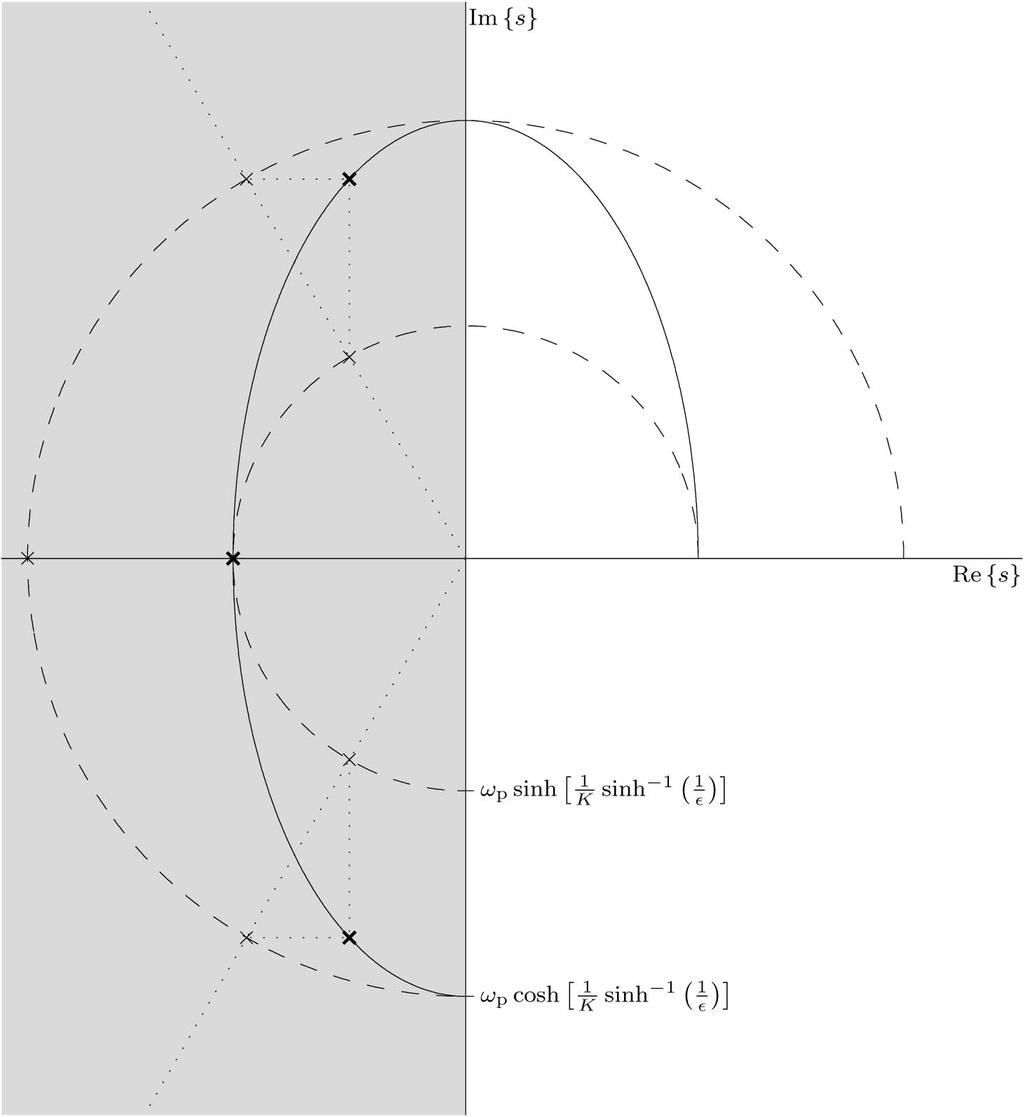
52 Determination of Chebyshev Poles and H(s) the Chebyshev filter poles, and thus its transfer function, are found by squaring the magnitude response, substituting ω = s/j to yield H(s)H( s), and then selecting the left half-plane denominator roots. Similar to how Butterworth poles lie on a semicircle, the poles of a Chebyshev lowpass filter lie on a semi-ellipse. There is a close relationship between pole locations on a Chebyshev ellipse and those on Butterworth circles: the real part of the Chebyshev poles coincide with those of an equivalentorder Butterworth filter with radius ω p sinh[1/k sinh -1 (1/ϵ)] and the imaginary part of the Chebyshev poles are equal to those of a Butterworth filter with radius ω p cosh[1/k sinh -1 (1/ϵ)].

54 Coefficients of normalized Chebyshev denominator polynomials

55 Coefficients of normalized Chebyshev denominator polynomials

56 Example Design the lowest-order Chebyshev lowpass filter that meets the specifications ω p 10 rad/s, α p 2 db, ω s 30 rad/s, and α s 20 db. Plot the corresponding magnitude response to verify that design requirements are met. Solution Step 1: Determine the filter order K from equation omegap = 10; alphap = 2; omegas = 30; alphas = 20; K = ceil(acosh(sqrt((10^(alphas/10)-1)/(10^(alphap/10)-1)))/acosh(omegas/omegap)) K = K = 2 Step 2: Determine the range for the passband cutoff frequency ω P by setting ω s = 30 and K = 2 and solve the above equation for ω P. omegap = [omegap,omegas/cosh(acosh(sqrt((10^(alphas/10)-1)/(10^(alphap/10)-1)))/k)] ω P = Choose the average so ω P =

57 Continue Example Step 3: Determine the prototype lowpass filter transfer function H(s) First we find ϵ, H(j0), poles, and then the lowpass prototype epsilon = sqrt(10^(alphap/10)-1); k = 1:K; H0 = (mod(k,2)==1)+(mod(k,2)==0)/sqrt(1+epsilon^2); pk = -omegap*sinh(asinh(1/epsilon)/k)*sin(pi*(2*k-1)/(2*k))+... 1j*omegap*cosh(asinh(1/epsilon)/K)*cos(pi*(2*k-1)/(2*K)); B = H0*prod(-pk), A = poly(pk) H(0) = B = H(0) *p 1 *p 2 = A = [ ] HH ss = ss ss Alternatively, the lowpass-to-lowpass transformation s s/ω p = s/ applied to the appropriate coefficients of Table 2.4 yields the same denominator

58 Continue Example omega = linspace(0,35,1001); H = B./(polyval(A,1j*omega)); plot(omega,abs(h)); HH ss = ss ss

59 Example Design the lowest-order Chebyshev bandstop filter that meets the specifications ω P1 5 rad/s, ω P2 35, α p 2 db, ω s1 10 rad/s, ω s2 20 and α s 20 db. Plot the corresponding magnitude response to verify that design requirements are met. Solution Step 1: Determine the Lowpass Prototype First we normalize the stopband frequency ω S = 1 and then we calculate the passband frequency ω P for both transition bands of the bandpass filter and choose the most restrictive ω P. omegap1 = 5; omegap2 = 35; omegas1 = 10; omegas2 = 20; omegas = 1; omegap = abs([omegas*(omegap1*(omegas2-omegas1))/(-omegap1^2+omegas1*omegas2),... omegas*(omegap2*(omegas2-omegas1))/(-omegap2^2+omegas1*omegas2)]) ω P = To meet the specifications of both transitions we choose the most restrictive which is the upper transition band, so ω P = , this will lead to a higher order filter K.

60 Continue Example Next we determine the filter order K from equation omegap = max(omegap); alphap = 2; alphas = 20; K = ceil(acosh(sqrt((10^(alphas/10)-1)/(10^(alphap/10)-1)))/acosh(omegas/omegap)) K = 2 Determine the range for the stopband cutoff frequency ω S by setting ω P = and K = 2 and solve the above equation for ω S. omegas = mean([omegas,... omegap*cosh(acosh(sqrt((10^(alphas/10)-1)/(10^(alphap/10)-1)))/k)]) omegas = Choose the average to provide both passband and stopband buffer zones, so ω S =

61 Continue Example Next, since we adjusted ω S we recalculate ω P using the equation omegap = omegas/cosh(acosh(sqrt((10^(alphas/10)-1)/(10^(alphap/10)-1)))/k); omegap = ω P = Step 3: Determine the lowpass prototype filter transfer function H(s) First we find ϵ, H(j0), the poles, and then the lowpass prototype epsilon = sqrt(10^(alphap/10)-1); k = 1:K; pk = -omegap*sinh(asinh(1/epsilon)/k)*sin(pi*(2*k-1)/(2*k))+... 1j*omegap*cosh(asinh(1/epsilon)/K)*cos(pi*(2*k-1)/(2*K)); H0 = mod(k,2)+mod(k+1,2)/sqrt(1+epsilon^2); B = H0*prod(-pk), A = poly(pk) H(0) = B = H(0) *p 1 *p 2 = A = [ ] HH ss = ss ss

Continue Example Step 4: Determine the bandpass filter transfer function H(s) by transformation HH ss = 0.0846 ss 2 + 0.

62 Continue Example Step 4: Determine the bandpass filter transfer function H(s) by transformation HH ss = ss ss ss 10ss ss HH ss = ss ss ss ss ss ss

63 Continue Example (Matlab Code) omegap1 = 5; omegap2 = 35; omegas1 = 10; omegas2 = 20; omegas = 1; omegap = abs([omegas*(omegap1*(omegas2-omegas1))/(- omegap1^2+omegas1*omegas2),... omegas*(omegap2*(omegas2-omegas1))/(-omegap2^2+omegas1*omegas2)]) omegap = max(omegap); alphap = 2; alphas = 20; K = ceil(acosh(sqrt((10^(alphas/10)-1)/(10^(alphap/10)-1)))/acosh(omegas/omegap)) omegas = mean([omegas,... omegap*cosh(acosh(sqrt((10^(alphas/10)-1)/(10^(alphap/10)-1)))/k)]) omegap = omegas/cosh(acosh(sqrt((10^(alphas/10)-1)/(10^(alphap/10)-1)))/k); epsilon = sqrt(10^(alphap/10)-1); k = 1:K; pk = -omegap*sinh(asinh(1/epsilon)/k)*sin(pi*(2*k-1)/(2*k))+... 1j*omegap*cosh(asinh(1/epsilon)/K)*cos(pi*(2*k-1)/(2*K)); H0 = mod(k,2)+mod(k+1,2)/sqrt(1+epsilon^2); B = H0*prod(-pk), A = poly(pk) a = 1; b = -(omegas2-omegas1)./pk; c = omegas1*omegas2; B = B/prod(-pk)*poly([1j*sqrt(c)*ones(K,1);-1j*sqrt(c)*ones(K,1)]) A = poly([(-b+sqrt(b.^2-4*a.*c))./(2*a),(-b-sqrt(b.^2-4*a.*c))./(2*a)]) omega = linspace(0,100,1001); H = polyval(b,1j*omega)./polyval(a,1j*omega); plot(omega,abs(h));

64 Inverse Chebyshev Filters Type II The magnitude response exhibits a maximally flat passband and an equiripple stopband. While Butterworth and Chebyshev type 1 filters have finite poles and no finite zeros, the inverse Chebyshev has both finite poles and zeros. The presence of zeros enhance the frequency response but the decay rate for ω > ω s is slower. The inverse Chebyshev response can be obtained from a Chebyshev response in two steps. To begin, let H c (ω) be a lowpass Chebyshev magnitude response with passband edge ω p and ripple parameter ϵ, as shown in Fig. a. In the first step, we subtract H c (ω) 2 from 1 to obtain the response shown in Fig. b. In the second step, we interchange the stopband and passband with the lowpass-to-highpass transformation of ω ω p ω s /ω yields the inverse Chebyshev response, shown in Fig. c.

65 Elliptic Filters and Bessel-Thomson Filters Elliptic Filters Chebyshev filters have a smaller transition bands compared with that of a Butterworth filter because Chebyshev filters allow rippling in either the passband or stopband. Elliptic filter allows ripple in both the passband and the stopband, so it achieves a further reduction in the transition band. For a given transition band, an elliptic filter provides the largest ratio of the passband gain to stopband gain, or for a given ratio of passband to stopband gain, it requires the smallest transition band. Bessel-Thomson Filters Unlike the previous filters, where we approximate the magnitude response without paying attention to the phase response, the Bessel-Thomson filter is designed for maximally flat time delay over a bandwidth of interest. This means that the phase response is designed to be as linear as possible over a given bandwidth. Bessel-Thomson filters are superior to the filters discussed so far in terms of the phase linearity or flatness of the time delay. However, they do not fair so well in terms of the flatness of the magnitude response.

Analog Lowpass Filter Specifications

Analog Lowpass Filter Specifications Typical magnitude response analog lowpass filter may be given as indicated below H a ( j of an Copyright 005, S. K. Mitra Analog Lowpass Filter Specifications In the