The Pennsylvania State University. The Graduate School. Graduate Program in Acoustics TRADITIONAL AND ANGLE-DEPENDENT CHARACTERIZATION OF PENN

Transcription

1 The Pennsylvania State University The Graduate School Graduate Program in Acoustics TRADITIONAL AND ANGLE-DEPENDENT CHARACTERIZATION OF PENN STATE S PANEL TRANSMISSION LOSS SUITE A Thesis in Acoustics by Paul Bauch 2013 Paul Bauch Submitted in Partial Fulfillment of the Requirements for the Degree of Master of Science August 2013

2 The thesis of Paul Bauch was reviewed and approved* by the following: Stephen A. Hambric Thesis Advisor Professor of Acoustics Senior Scientist, PSU Applied Research Laboratory Andrew Barnard Thesis Advisor Research Associate, PSU Applied Research Laboratory Daniel Russell Professor of Acoustics Director of Distance Education, Graduate Program in Acoustics Michelle Vigeant Assistant Professor of Acoustics & Architectural Engineering Penn State University Victor Sparrow Interim Chair of The Graduate Program in Acoustics Professor of Acoustics *Signatures are on file in the Graduate School

3 iii ABSTRACT The Center for Acoustics and Vibration at Penn State has a Panel Transmission Loss Suite consisting of a reverberation chamber coupled to an anechoic room. This facility has multiple applications in sound attenuation metrics and sound radiation analysis. The facility was characterized to determine the performance and limitations of the space. The reverberation chamber was previously characterized according to ASTM C423-02a, with a cutoff frequency at 630 Hz and reverberation times from 3 to 7 seconds. The anechoic room has been characterized according to ISO 3745 (2003) over the frequency range of 160 Hz to 10 khz. The room behaves hemi-anechoically over this frequency range and meets the allowable deviation from the inverse square law for hemi-anechoic environments. Flanking transmissions have been measured according to ASTM E2249 and E90, limiting transmission loss measurements to 40 db at the 400 Hz one-third-octave band increasing to 55 db at the 10 khz band. The diffusivity of the incident sound field at the transmission aperture, or niche, has been investigated using beamforming and spatial correlation techniques. Transmission loss measurements suggest near-normal-incidence plane waves at frequencies below 1 khz transitioning to more random of field incidence at frequencies above 1 khz. Potential diffusivity metrics at the niche are discussed based on these measurements. The Spatial Correlation Assurance Function (SCAF) is introduced to quantify incident field diffusivity in transmission loss facilities. Deviations in the sound pressure level at the transmission aperture from the averaged sound pressure level in the source room may be used to correct the non-diffuse field bias in lower frequency bands.

4 iv TABLE OF CONTENTS List of Figures... vi List of Tables... ix Acknowledgements... x Chapter 1 Introduction Transmission Loss Facility Design Penn State s Transmission Loss Suite Facility Characterization from Standards Field Diffusivity at Transmission Aperture Scope of Thesis... 8 Chapter 2 Theory Definitions Anechoic Free Field Decay Image Source Method for a Rigid Infinite Baffle Panel Transmission Loss Sound Intensity Measurement Discrete Linear Array Time Domain Beamforming Spatial Correlation Function and Field Diffusivity Theory Chapter 3 Methodology Anechoic Chamber Characterization Setup Experimental Hardware ISO 3745 Qualification Experiment Anechoic Behavior Characterization Transmission Loss Measurements and Flanking Transmission Flanking Transmission Measurement Transmission Loss of Sample Panels Angular Dependent Incident Sound Field and Spatial Correlation Beamforming Field Incidence and Spatial Correlation Function Pressure Level Comparison Along Transmission Aperture Surface Chapter 4 Results Anechoic Room Characterization Results Flanking Path Analysis Pressure Deviations at the Transmission Aperture Panel Pressure Angular Dependence and Spatial Correlation Results Panel Transmission Loss Examples Chapter 5 Conclusions and Discussion... 59

5 v 5.1 Qualification Standards Transmission Aperture Incident Field Study Future Work and Suggestions Appendix A A.1 MATLAB coding for ISO 3745 results A.2 Normalized Pressure Results for Anechoic Room Traverse Paths Appendix B B.1 Field Indicator Determination B.1.1 Pressure-Residual Intensity Index and Dynamic Capability Index B.1.2 Field Indicators B.1.3 Qualification Criterion B.1.4 Intensity Probe Calibration Sheet Appendix C C.1 Effects of 1/3 Octave Filtering the Spatial Correlation Data and the SCAF Appendix D D.1 Omnidirectional Source Calibration Sheet... 88

6 vi LIST OF FIGURES Figure 1.1. Reverberation-Anechoic room Panel Transmission Loss Suite... 1 Figure 1.2. (a) Panel Transmission Loss Aperture with dimensions. Panels mount on visible side (anechoic environment). (b) Scale schematic of TL facility with source locations and dimensions... 3 Figure 1.3. Example Flanking Transmission Paths Figure 1.4. Schematic of the niche effect and incident field. Fields can be reversed by mounting the panel on the incident field side of the aperture Figure 2.1. Inverse square law for a simple source in a free-field. Surfaces represented in red should conform to the surface of a sphere enclosing the source Figure 2.2. Theoretical results of sound pressure level normalized to the source volume velocity. Constructive and destructive interference pattern is shown in hemianechoic case Figure 2.3. Model for hemi-anechoic environment showing the image-source method Figure 2.4. Generalized transmission loss model for a single layer wall. The frequency scale is logarithmic. Mass law theory yields a 6dB per octave or frequency doubling Figure 2.5. Coincidence effect. Bending wave wavelength in the panel is matched by incident airborne wavelength Figure 2.6. N-element linear array of equally spaced sources showing plane wave geometry Figure 2.7. Example beam pattern for 9-element array where kd= Figure 2.8. Examples of the steered beam pattern of the 9-element array where kd= Figure 3.1. Anechoic characterization experimental setup schematic Figure 3.2. (a) Physical traverse setup with microphone in cradle. (b) Anechoic traverse paths for room characterization. Dashed lines represent diagonal paths toward upper corners; solid lines represent paths parallel to floor at constant height Figure 3.3. Shielding configuration cases for flanking transmission measurement Figure 3.4. Intensity measurement grid for flanking transmission and transmission loss measurements Figure 3.5. Transmission aperture microphone array panel (top-left) and close-up (topright). Microphones fit into panel as shown in top-right and bottom image. The bottom image represents cross-correlation setup with reference microphone in the

7 vii center position, as viewed from the incident, reverberant, side of the panel. Holes were left open during all measurements Figure 4.1. Signal to noise levels for anechoic qualification measurements. Signal is 10 db higher than noise at all measurement points and all frequencies above 160 Hz Figure 4.2. Room performance within allowable deviation from ISO Data collected in January 2012 (panel fluorescent lights installed covered with wedges) Figure 4.3. Room performance within allowable deviation from ISO Data collected in January 2013 (6 small compact fluorescent lights installed) Figure 4.4. Sample comparison with hemi-anechoic theory for traverse path 2 position 7. Levels are normalized to the source strength and do not represent actual sound pressure levels Figure 4.5. Criterion 1 of ISO surface pressure-intensity indicator. Measured signals are less than the dynamic capability index Figure 4.6. Criterion 2 of ISO field non-uniformity indicator. For higher transmission loss cases, the field is less uniform due to contributions from flanking paths. This criterion ensures that a sufficient number of measurement points were used in the measurement surface. The red dashed line represents the 36-point measurement array used in this study Figure 4.7. Flanking transmission experiment results. Solid red line shows the upper limit on transmission loss metrics based on 10 db down from flanking levels Figure 4.8. Sound pressure level normalized to max one-third octave aperture pressure at the transmission surface. Horizontal (a) and vertical (b) arrays show similar results in respective third octave bands Figure 4.9. Narrowband beamforming results as a function of steered angle (incidence angle). Horizontal axis (top) and vertical axis (bottom). Stronger incident sound energy occurs at various angles of incidence and frequencies Figure Narrowband normalized beamforming results as a function of steered angle (incidence angle). Levels are relative to normal incidence (0 ). Horizontal axis (top) and vertical axis (bottom). Vertical red and yellow strips indicate potential resonance effects in the room Figure Horizontal (top) and vertical (bottom) beamforming results normalized to normal incidence for the 400 Hz, 500 Hz, 630 Hz, 800 Hz, and 1 khz one-third octave bands. Illustrations on the right show beam steering direction. Sinusoidal shape indicates standing waves or resonances in the aperture or room Figure Mid-frequency horizontal (top) and vertical (bottom) beamforming results for 1.25 khz to 3.15 khz one-third octave bands. Vertical data shows assumed field

8 incidence conditions with taper off around 78 degrees angle of incidence in agreement with Figure Figure High-frequency results for horizontal (top) and vertical (bottom) arrays. Peak in the horizontal plane at -20 degrees angle of incidence suggests direct field from one of the sources. Vertical array data shows similar peaks which could indicate direct field reflections Figure Ray tracing method illustrating the direct field influence of the higher frequency source Figure Incidence angle tolerances derived from one-third octave band limited beamforming data. Horizontal axis (top) shows tighter solid angles above 4 khz. Similar results are shown for vertical axis (bottom), with decreased beamwidth below frequencies of 1kHz Figure Incidence angle beamwidth within tolerance shown for horizontal axis (top) and vertical axis (bottom). Random incidence is indicated between 1.25 khz and 4 khz with a 3 db tolerance Figure Spatial correlation results for each one-third octave band as a function of kr. The horizontal axis (top) and the vertical axis (bottom) show good agreement for low values of kr. The sign of kr denotes direction in transmission aperture (-) is away from the wall and towards the ceiling Figure Spatial correlation results for each one-third octave band as a function of kr at small kr. The horizontal axis (top) and the vertical axis (bottom) show good agreement for low values of kr Figure SCAF results for horizontal (top) and vertical (bottom) arrays. Results shown were filtered into 1/3 octaves before applying the SCAF. Sample spatial correlation function data at the 500 Hz to 6.3 khz one-third octave bands are shown to illustrate how the SCAF value evaluates the level of agreement in the spatial correlation results Figure Transmission loss for 3.18 mm high density fiberboard (HDF) with 95% confidence compared with mass law theory (dashed lines). The vertical dashed line represents the theoretical coincidence frequency, which agrees with measured data. Solid green line indicates limitation from flanking transmission levels Figure Transmission loss for 1.5 mm steel panel with 95% confidence compared to mass law theory Figure Criterion 1 from ISO for HDF and steel transmission panel measurements Figure Criterion 2 from ISO for HDF and steel transmission panel measurements viii

9 ix LIST OF TABLES Table 3-1. ISO 3745 qualification specifications for hemi-anechoic rooms... 26

10 x ACKNOWLEDGEMENTS I would like to thank my research advisor, Dr. Andrew Barnard, for his endless support and direction in this study. His contributions and suggestions were vital in the characterization process. Dr. Barnard also provided some of the LabVIEW programming and MATLAB code that was used throughout my research. As an entry-level researcher, I have gained much from his guidance and understanding of acoustics. I would also like to thank my committee for reviewing this thesis and providing guidance and suggestions. My parents have also been a source of support and love that has provided me with motivation and endurance throughout my education. I am forever thankful for them and my brothers and their families and of course my extended family. Thank you all so much. Much thanks and acknowledgment goes to the employees involved with my research at the CAV and ARL. Rick Auhl was very supportive in managing and lending the lab equipment to me. His team even helped remove the massive door on the transmission aperture and a few weeks later put it back on. Micah Shepherd, who provided insight for the transmission loss measurements including code for theoretical results and the use of a software package that assured I was on the right track. I would also like to thank the students, faculty and staff in the Graduate Program in Acoustics, many of whom provided a means to discuss ideas, methodology and professional development. I ve gained much from the friendships, networks, and collaborations and I expect the benefits of these relationships will continue as I progress through life.

11 Chapter 1 Introduction The Center for Acoustics and Vibration (CAV) at the Pennsylvania State University has a Panel Transmission Loss (PTL) facility, illustrated in Figure 1.1. Panel transmission loss is the difference between the sound power incident on a panel and the sound power transmitted through that panel [1] [2] [3]. The CAV facility is constructed of a reverberation chamber adjoined to an anechoic room with a common wall. This shared wall contains an opening for mounting various panels for transmission loss testing. This thesis further characterizes the facility for use as a transmission loss suite, building on the reverberation chamber characterization performed by Orr [4]. The characterization is achieved using current standards and techniques for quantifying reverberation chambers, anechoic environments, and transmission walls. Angular dependent field diffusivity at the transmission aperture is also investigated using spatial filtering in the frequency domain. Figure 1.1. Reverberation-Anechoic room Panel Transmission Loss Suite.

12 2 1.1 Transmission Loss Facility Design Transmission loss facilities have many uses. Reverberation chambers are instrumental in a variety of acoustic measurements ranging from absorption coefficients of materials to source characterization [5]. A reverberation chamber is designed to have large reverberation times through the use of highly reflective materials such as concrete or metal. Conversely, anechoic chambers simulate a free field environment in which sound measurements such as source directivity can be made [6]. The free field of an anechoic room is achieved by minimizing sound reflection from the surfaces of the room. Absorptive neoprene foam or fiberglass wedges cover surfaces to prevent reflections. Anechoic rooms can be either full- or hemi-anechoic. Fullanechoic environments have absorptive surfaces on all sides of the room, including the floor, and have a suspended mesh floor for walking and mounting equipment. In contrast, hemi-anechoic rooms have a rigid floor that reflects sound. The coupling of a reverberation chamber to an anechoic space through an aperture is ideal for transmission loss measurements. The facility is separated into the source room, where sound is generated, typically the reverberation chamber, and a receiver room, where the sound transmission is measured, which can be either a second reverberation chamber or anechoic room. A transmission loss measurement is related to the difference in energy between the two rooms. This can be measured using an intensity probe according to the standard ASTM E [2] [3]. The transmission loss suite is vital for noise control industries. With improving passenger comfort as a primary goal aerospace and automotive companies are investing in accurate methods for measuring transmission loss. Transmission loss facilities are used by these industries to analyze airborne sound transmission through cabin panels and other structures.

13 3 1.2 Penn State s Transmission Loss Suite The CAV PTL facility (Figure 1.1) has a square opening (0.89m x 0.89m x 0.15m) on the shared wall between the two rooms. This reverberation chamber is 6.71 m x 5.69 m x 3.47 m with an isolated concrete slab floor. The walls are painted cinderblock and the ceiling consists of metal decking which is more absorbent than the other surfaces. Atmospheric absorption in the chamber begins to increase significantly above 4 khz [4]. The anechoic room is rectangular (4.95 m x 3.84 m x 2.95 m) with a 1 m x 0.5 m cutout where the door is located. It has a semi-rigid carpeted plywood floor. The entire room is elevated 0.5 m above a tiled concrete floor. The dimensions of the room are measured from wedge-tip to wedge-tip. Wedges are 30 cm x 30 cm x 61 cm acoustic foam tetrahedrons with wedge depth of 38cm. The reverberation chamber entrance is located on the common wall. Figure 1.2 is the PTL aperture as seen from the anechoic receiver room and a scale drawing of the entire facility showing the source locations used in PTL metrics. Panels are mounted to the aperture on the anechoic side. The facility is also equipped with a ceiling mounted turntable in the reverberation chamber for mounting diffusers or moving microphones. Figure 1.2. (a) Panel Transmission Loss Aperture with dimensions. Panels mount on visible side (anechoic environment). (b) Scale schematic of TL facility with source locations and dimensions. Note: The aperture door does not lay flat against reverberation room wall.

14 4 1.3 Facility Characterization from Standards To completely characterize the facility, several metrics must be evaluated. These specifications will detail the limitations in the performance of the facility. While much is known and standardized for reverberation and anechoic rooms independently, the only specification for PTL facilities is for flanking paths [2] [7]. Flanking paths refer to noise transmitted through structures and surfaces not in the measurement surface. Figure 1.3 illustrates some possible flanking paths including floors, walls, door seals and aperture fixture. Typically, the aperture depth causes the incident field to be less diffuse, changing intensity with angle of incidence. Consideration for angular diffusivity, the deviation in field level over incident angle, has been generally avoided with the exception of a study investigating a phenomenon known as the niche effect [8], an experimental study of angular dependence by H.J. Kang [9] and the PhD thesis by M.J. Daley analyzing spatial field discrepancies on the surface of a small reverberant environment [10]. The niche effect is the apparent increase in transmission due to reflections from the features of the aperture. Figure 1.4 illustrates this niche effect. Kang wrote another paper suggesting a technique for more accurate sound transmission loss predictions of multi-layered panels. Kang s new prediction method adjusts for the distribution of directional incident energy at the surface of the panel [11]. Figure 1.3. Example Flanking Transmission Paths.

15 5 Figure 1.4. Schematic of the niche effect and incident field. Fields can be reversed by mounting the panel on the incident field side of the aperture. The diffusivity of a reverberation chamber can be characterized by the reverberation time or decay rate, the rate at which the sound energy decreases. The procedure for determining reverberation time for a reverberation room is presented in ASTM E [5]. The standard requires at least 50 decay rate measurements, where the source is turned off from steady state, while measuring the average sound pressure level throughout the room. Decay begins 100 to 300 ms after the source is turned off. A theoretical approximation of the Schroeder frequency, the frequency above which the room is modally dense, has also been used to determine the performance of a reverberation chamber [1] [4] [12]. Modal analysis has also been used to model the response of a reverberation room in comparison with the ASTM procedure. This work was previously completed for the CAV facility by Orr in 2011 and detailed in his thesis, Characterization of the Center for Acoustics and Vibration Reverberation Chamber [4].

16 6 Anechoic environments are designed to simulate a free field. A simple source should respond according to the inverse square law (spherical spreading) in such an environment. ISO details a procedure for determining how well a space follows this law [6]. Microphone traverse paths are set up to measure the sound pressure level at various distances from the source. The standard contains averaging techniques for comparing the room s performance to spherical spreading within acceptable deviations. Since an anechoic room greatly reduces, or eliminates, reflections, a measure of reverberation time is not an accurate metric for characterization. Consideration for the reflective behavior of hemi-anechoic rooms in the standard increases the acceptable deviation from spherical spreading. Cunefare studied anechoic chamber qualification methods and found inadequacies in the standard and also suggested best practices [13]. Specifically, broadband sources are better fitted for discrete microphone traverses. The rigid floor and assumption of a spherical or simple source allows a model to be created using the technique of image sources [12]. In the case of a hemi-anechoic space there will be one image source, mirrored by the rigid floor, for each source in the room. Sound energy can penetrate from the source room into the receiver room through a number of paths known as flanking paths as shown in Figure 1.3. The flanking transmission is the level of noise that exists in the receiver room when the source room is acoustically excited and the transmission aperture is filled with a large amount of shielding. This flanking noise can limit the facility s ability to measure higher transmission losses since the flanking transmission increases the background level in the receiver room. Both E and ASTM E90-02 provide a method for measuring flanking transmission. The usable measurement limit for transmission loss is 10 db below this flanking transmission loss [2] [7]. Power levels are measured on the anechoic side at the aperture with an intensity probe, which uses two phase-matched microphones. Frequency domain intensity is measured from the cross-spectrum of the two microphone signals [14]. The spatial averaged intensity measurement accuracy is verified using the standard ISO

17 for discrete measurement points [15]. Parts 2 and 3 of ISO 9614 are specific to continuous scanning methods [16] [17] Field Diffusivity at Transmission Aperture In general, very little has been done to characterize the field near the aperture. Two known studies have taken different approaches. The paper on the niche effect by Tetsuya Sakuma implements numerical vibro-acoustics analysis of several window designs with varied conditions on the window depth related to incidence and transmission [8]. The study found a bias due to reflections on the edge of the niche. According to Sakuma, the worst case exists when the panel divides the aperture depth in half. The experimental study by Kang investigated this effect with the use of an intensity probe mounted in the aperture with a rotating fixture [9]. The probe could measure the intensity at any angle in the hemisphere created by the partition. Results showed lower intensity at higher angles of sound incidence. The combination of these two studies led to the conclusion that the incident field at the aperture is not truly diffuse. Some problems do arise with the implementation of an intensity probe. The size of the probe itself and the size of the opening to mount and rotate the probe create conditions that would not exist if the aperture were filled with a test panel. There is still a need for a practical method that will quantify a facility s limitation due to angular variation in the incident field and adjust transmission loss metrics for these conditions. Spatial filtering beamforming can be used for angular dependent sound level measurements to achieve the target metric. This technique processes signals from an array of receivers to steer a main beam in any direction in the plane of the array. Mucci presents several methods for implementing beamforming in both the time- and frequency-domain [18]. Similar methodology

18 8 can be found in the technical report on linear arrays by Hampson [19]. Limitations due to number of receivers can be avoided by working in the frequency domain. A similar spatial filtering technique compares the level deviation across an array through cross correlation. The PhD thesis by Mike Daley introduces the concept of using spatial correlation applied to surfaces in reverberant environments [10]. In this thesis, the spatial filtering techniques will be adapted to measuring the angle dependent incident sound field at the transmission aperture. Furthermore, a spatial correlation assurance function (SCAF) for characterizing similar facilities based on spatial correlation functions and measured data is proposed. The SCAF is similar in application to the modal assurance criterion (MAC), which is a check for linearity between two modal vectors [20]. The SCAF uses the same vector mathematics in comparing the similarity between theoretical spatial correlation and measured data. The current standard for measuring sound transmission loss using the intensity method derives the incident sound intensity on the surface of the panel from the average sound pressure level in source room [2] [3] [21]. Corrections for the non-diffuse behavior of the sound field at the transmission aperture are generally ignored. These deviations are increased when the transmission aperture has depth where the niche effect exists [8] [9]. Using the average sound pressure level at the surface of a panel mounted in the transmission aperture the sound field at the surface can be measured showing the influence of the niche effect. 1.5 Scope of Thesis Chapter 2 discusses the theory behind the techniques used in this thesis. This includes free-field decay and the inverse square law, frequency dependent sound intensity measurements, and spatial filtering using discrete linear arrays (beamforming and spatial correlation). Chapter 3 covers the methodology for experimental analysis of anechoic environment characterization,

19 9 flanking transmission limitations, and diffuse field incidence variations through spatial filtering. Equipment, processing methods, and data acquisition parameters for each measurement technique are discussed. Results of these measurements are presented in chapter 4. The measurements of anechoic behavior and flanking transmission are presented in accordance with applicable standards. Experimental limitations are shown, providing limits of use on the facility. Results from beamforming and spatial correlation techniques are also presented and discussed. These results provide reasonable criteria for defining angles of incidence in which the sound field is diffuse. Usable incidence angles for the TL suite are presented based on these criteria. The sound pressure levels across the transmission aperture are presented suggesting niche effect influence at the aperture. The final chapter discusses conclusions focusing on the transmission aperture incident sound field. A standard practice is proposed for quantifying transmission loss facilities based on spatial filtering analysis and the spatial correlation assurance function of the transmission aperture.

20 Chapter 2 Theory 2.1 Definitions Some common quantities in acoustics include sound pressure, intensity, and power. These quantities are often expressed as logarithmic levels on a decibel scale compared to a reference quantity. The sound pressure level, L p, intensity level, L I, and sound power level, L W, are defined respectively as (2.1) (2.2) (2.3) where p is the root mean square sound pressure and p 0 the reference pressure, 20 μpa. Intensity is I and the reference intensity, I 0, is equal to W/m 2. Sound power is denoted by W and the reference power is W 0, W. Other common variables include the acoustic wave number, k, and frequency, f, which are related by the wavelength, λ, and speed of sound under ambient conditions, c 0, by (2.4) where ω is the angular frequency,. [12] The methodologies in this thesis use several spectral analysis methods. The autospectrum, G 11, is defined as

21 11 (2.5) where p 1 (t) is the time-domain pressure signal from a microphone and S is the Fast Fourier Transform (FFT) of the signal. The (*) denotes the complex conjugate. Similar to the autospectrum, the cross-spectrum is defined as (2.6) where p 2 (t) is the time-domain pressure signal from a second microphone recorded simultaneously with the first. Another two channel signal analysis tool is the frequency response function (FRF). The FRF is the frequency domain ratio of two signals, defined by (2.7) where the G 12 (ω) is the cross-spectrum of channel 1 and channel 2 and G 11 (ω) is the autospectrum of first channel, often referred to as the reference channel. 2.2 Anechoic Free Field Decay A simple source in an anechoic environment will exhibit free field decay where the sound intensity level decreases by 6 db per doubling of distance. This is due to spherical spreading of the sound field. Sound radiating from a spherical point source obeys the inverse square law. For a point source, in a free-field, that has an output sound power level, W, the sound intensity, I, at some distance, r, away from the source can be expressed as (2.8) Figure 2.1 shows the physical mechanism that occurs with spherical radiation.

22 12 Figure 2.1. Inverse square law for a simple source in a free-field. Surfaces represented in red should conform to the surface of a sphere enclosing the source. 2.3 Image Source Method for a Rigid Infinite Baffle modeled as In an anechoic environment the steady state pressure from a simple source can be (2.9) where ρ 0 is the ambient density of air, Q the volume velocity of the source, and r is the distance from the source [12]. Similarly, a simple source near an infinite baffle can also be modeled by assuming a mirror image of the source on the other side of the barrier. Both sources provide a pressure field equivalent to equation 2.9. Due to the superposition of these two in-phase sources, pressure doubling occurs at the boundary. It is useful to normalize the pressure, p(r), by the volume velocity, Q. For the purpose of this study the complex number, j, can be lumped into the volume velocity. For a simple source in a fully anechoic environment this normalization is (2.10) Due to the interference pattern from the reflective surface, the sum of the direct and reflected sound will show constructive and destructive interference depending on frequency,

23 receiver location and the distance between the source and the reflective surface. Using the image source method and combining two in-phase sources the normalized sound pressure is 13 (2.11) where r 1 is the distance between the real source and the receiver and r 2 is the distance between the image source and the receiver. Equation 2.11 is the normalized pressure for a source near an infinite baffle [12]. Figure 2.2 shows the results of Equation 2.10 and Equation The model for a source in a hemi-anechoic field shows the constructive and destructive interference pattern. For the purposes of this paper the floor of the anechoic room will be modeled as an infinite baffle. Figure 2.3 illustrates the image source in a hemi-anechoic environment. Figure 2.2. Theoretical results of sound pressure level normalized to the source volume velocity. Constructive and destructive interference pattern is shown in hemi-anechoic case.

24 14 Figure 2.3. Model for hemi-anechoic environment showing the image-source method. 2.4 Panel Transmission Loss A panel separating two acoustic environments will attenuate sound as a function of frequency. A panel s transmission loss (TL) is defined by several frequency regions. These regions include stiffness controlled, resonance, mass controlled, coincidence or damping controlled, and shear controlled regions, respectively increasing with frequency [1]. Figure 2.4 shows an example plot of TL. Each region can be predicted with simplified equations. The stiffness and resonance regions are governed by the restoring force and damping within the material.

25 15 Figure 2.4. Generalized transmission loss model for a single layer wall. The frequency scale is logarithmic. Mass law theory yields a 6dB per octave or frequency doubling. For a finite panel the first resonance frequency is expressed as (2.12) where a and b are the dimensions of the panel and m s is the surface mass density of the panel. The bending stiffness of the panel, B, is derived from the young s modulus, E, and poisson s ratio, σ, defined as (2.13) where h is the thickness of the panel. An approximation of the TL below the first resonance frequency in the stiffness-controlled region, from Sharp, is [1] (2.14)

26 16 for frequencies up to the first natural frequency, f 1. The 47.3 db in equation 2.14 is a numerical constant that contains the metric acoustic properties of the air, the speed of sound and the density. The next frequency region is controlled by the inertia of the panel. The mass law predicts the TL in this region. Assuming a diffuse field with incidence angles between 0 and 78 leads to field-incidence TL, defined in the low-frequency mass law region for metric units as (2.15) where the TL is very predictable. An increase of 6 db per octave is expected. A TL model can also be made using plane wave sound fields incident at a variety of angles. The mass law for these cases takes the form (2.16) where θ p is the plane wave incidence angle, measured from normal incidence. A plane wave incident on the panel will still have a TL increase of 6 db per octave, but have a different offset than Equation A thin panel in a diffuse field where airborne grazing incidence waves match the bending mode wavelengths of the panel will yield a drop in TL known as the coincidence dip. The increased transmission is due to the reradiated sound power through excited bending waves. Figure 2.5 shows the wavelength matching and radiation from bending waves of a thin panel in a diffuse field. The lower limit of the matching frequency is known as the critical frequency and is defined as (2.17) The incident airborne frequency is related to the critical frequency by (2.18)

27 17 This is the coincidence frequency related to angle of incidence, θ. The coincidence effect only occurs above the critical frequency due to the angular dependence [1]. The diffuse field TL in this region is estimated by Fahy [1] as (2.19) where the panel s loss factor or damping coefficient, η, is a material specific quantity. The loss factor indicates bending wave damping in the panel. Figure 2.5. Coincidence effect. Bending wave wavelength in the panel is matched by incident airborne wavelength. 2.5 Sound Intensity Measurement The instantaneous sound intensity of an acoustic wave is a measure of magnitude and direction related to the acoustic pressure and particle velocity. The time-averaged intensity can be defined as (2.20)

28 18 where p is the instantaneous pressure and the instantaneous particle velocity containing magnitude and direction. T is the averaging period. For a plane or spherical harmonic wave travelling in some direction in the far-field, the time-averaged sound intensity is (2.21) The sign is dictated by the direction of the wave depending on the imposed coordinate system. Intensity is measurable in the frequency domain using two phase-matched pressure sensors spaced by a distance, d, through (2.22) where is the cross-spectrum between the two microphones [14]. The microphone closer to the source is p 1 and the microphone closer to the probe or farthest from the source is p 2. This orientation is important in determining the direction of the intensity vector. 2.6 Discrete Linear Array Time Domain Beamforming A linear array of transducers can be used as a directional source or receiver by applying simple signal processing techniques. Using an N element array of evenly spaced, identical simple sources as an example, the sound pressure at some point in the far field [12] is (2.23) where r i is the location of the point in the far field relative to each array element and the amplitude of each source is A. Figure 2.6 shows an example array of sources. For a linear array of length L and spacing d such that where, as shown in Figure 2.6,

29 19 the distance away from the center of the array source becomes and the resulting pressure becomes (2.24) which simplifies to (2.25) The maximum possible pressure amplitude is then (2.26) The pressure as a function of the incident angle of the summed array becomes a product of this maximum pressure and a directivity factor defined as (2.27) Figure 2.6. N-element linear array of equally spaced sources showing plane wave geometry.

30 20 Figure 2.7 shows the output beam pattern of a 9-point array with spacing such that kd=2 where the maximum pressure is located at broadside (0 ) incidence. This directional factor defines the beam shape. The real shape is three dimensional so that the broadside lobe creates a toroid-like shape. Figure 2.7. Example beam pattern for 9-element array where kd=2. Some applications require rotating or scanning the main beam without physically rotating the array. The beam can be electronically steered by applying a variety of signal processing techniques. In the time domain, the addition of a time delay into the signal for each source or transducer produces a steerable beam. The pressure signal for each source becomes (2.28) where the time delay,, equals, where ψ 0 is the desired steered angle from broadside incidence. The directional factor is now

31 21 (2.29) Figure 2.8 shows several examples of the steered beam using the same 9-element array with kd=2 as Figure 2.7. The beamwidth of the main lobe becomes larger as the beam is steered away from broadside. This phenomenon can be corrected using the directivity index explained in section of this thesis. Figure 2.8. Examples of the steered beam pattern of the 9-element array where kd= Spatial Correlation Function and Field Diffusivity Theory A sound field incident on a surface is considered diffuse if the spatial correlation function is equal to that of diffuse field theory. A diffuse field is a sound field that has an equal energy density at all locations in the field and equal probability of sound propagation in all directions. This means that the sound field near any source will not be diffuse. Assuming plane waves are

32 incident on the surface, the spatial correlation function, ρ, becomes a function of the pressure at two locations, 22 (2.30) where x 1 and x 2 are the locations where the averaged pressures,, are measured. For a linear array on a flat surface this function becomes a function of cross-spectra and auto-spectra referencing the pressure at the center location. For two pressure transducers, one at the center and the other traversing the length of the discrete array, equation (2.30) takes the normalized form, (2.31) where (2.32) and is the average cross-spectrum of the two pressures. The auto spectrum for the center position pressure sensor and pressure sensor at location, i, are and respectively. The distance between the two pressure transducers is x 1,2i. A diffuse pressure field will be isotropic such that the two auto-spectra are equal at all points [10].

33 23 Chapter 3 Methodology 3.1 Anechoic Chamber Characterization Setup The anechoic characterization experimental setup used the methods described in ISO 3745 [6]. This setup design investigated the behavior of the sound field in the anechoic chamber using two different measurements techniques. The first of these measurements followed the standard closely while the second looked at the anechoic or hemi-anechoic behavior at each discrete data point. The result is characterization according to ISO 3745 with further understanding of the sound field throughout the chamber Experimental Hardware A single source, a Brüel & Kjær dodecahedron OmniPower sound source type 4292, was used covering the frequency range of 100 Hz to 5 khz. The source provided a nearly flat response in a near-spherical pattern to imitate a simple monopole point source. A calibration sheet is shown in Appendix D. The type 4292 has twelve 5 speakers wired in parallel and series for impedance matching to the amplifier. The speakers were located around the surface of the dodecahedron enclosure. A compression driver, B&C 1050 driver with Beyma TD360 horn, was used as a second source to cover frequencies up to 10 khz. The sources were powered by a Crown XTi 2000 amplifier. The amplifier provided up to 475 Watts per channel at 8 ohms. A PCB Piezotronics Model 377B02 free-field microphone with ±1 db frequency response from 5 Hz to 10 khz connected to a model 426E01 preamplifier was set in a cradle attached to a traverse path constructed of a thin nylon string and pulley. The output signal from the amplifier, band

34 24 limited white noise in the range of 50 Hz to 10 khz, was attenuated 20 db before the signal was sent to the data acquisition device. A second Model 377B02 microphone was used as a reference microphone 1.5 m from the source to ensure consistent source output levels. Signals were acquired through a NI 9234 dynamic signal analyzer and a NI CompactDAQ 4-Slot USB chassis (cdaq-9174). Amplifier output (reference channel), traverse microphone, and reference microphone signals were collected simultaneously and both time history and frequency response data were recorded. Figure 3.1 illustrates the experimental setup. Figure 3.1. Anechoic characterization experimental setup schematic ISO 3745 Qualification Experiment The source was placed at the center of the anechoic room and elevated 1.3 meters above the floor. Measurements were based on the physical center of the source. Using twelve traverse paths the microphone was placed 0.7 meters from the source s center. This position was the starting point for each traverse path. Figure 3.2 illustrates the traverse paths used in this experiment. Data were collected including the physical position of the microphone using the center of the floor directly below the source as the origin. The microphone was then moved away

35 from the source in 0.3 m increments and the data were collected again. This process was repeated until the microphone was within 0.5 m of the anechoic walls. 25 Figure 3.2. (a) Physical traverse setup with microphone in cradle. (b) Anechoic traverse paths for room characterization. Dashed lines represent diagonal paths toward upper corners; solid lines represent paths parallel to floor at constant height. At each position along the traverse, twenty-five averages of 2.56 seconds were recorded using NI LabVIEW which provided a frequency resolution of 0.39 Hz. The sampling rate was 25.6 khz resulting in a usable frequency bandwidth of 10 khz. The LabVIEW program saved a.txt file containing the time-series and averaged frequency domain data. The auto-spectra, frequency response functions, and final time-series data are exported for processing in MATLAB. ISO 3745 uses a special averaging technique where a space is quantified by deviations from spherical radiation as where L pi is the sound pressure level at the ith position and L p (r i ) is the expected pressure according to the inverse square law. This expected sound pressure level is a function of the measured position and pressure at each traverse location; (3.1)

36 26 (3.2) where (3.3) and r 0 is the collinear offset of the acoustic center along the traverse, (3.4) where q i is the sound pressure at the ith position, r i is the distance of the ith position from the source center and N is the total number of measurements for each traverse. Table 3-1 provides the allowable deviations from spherical radiation according to the standard [6]. Section A1 of Appendix A details the processing outlined in ISO 3745 including the MATLAB code used in this study. Table 3-1. ISO 3745 acceptance criteria for hemi-anechoic rooms Frequency Range [Hz] Allowable Deviation [db] < 630 ± to 5,000 ±2.5 > 6,300 ± Anechoic Behavior Characterization The ISO 3745 standard does not allow for analyzing and distinguishing between a hemianechoic and full anechoic environment. More information about the anechoic behavior can be achieved using the same experimental setup for the ISO 3745 experiment. The frequency response functions referencing the amplifier output were stored. The volume velocity of the source was measured in a fully anechoic environment and used to normalize the sound pressure

37 27 levels at each traverse point. This normalization was done using the frequency response function of the measurement microphone located 1 meter from the center of the source with reference to the voltage into the source such that (3.5) where r is the distance between the microphone and source center and V in is the signal from the amplifier. In this case,. Combining this relationship with subsequent traverse measurements the sound pressure level normalized to source volume velocity, Q, is calculated by (3.6) The normalized pressure was compared to theoretical results discussed in section 2.2 using the microphone positions as the vector location of the receiver. This method provides significant advantages for analyzing the anechoic environment as compared to the ISO 3745 standard. Since the pressure is normalized, the sensitivity of the microphone and voltage attenuator is irrelevant as long as they are kept constant throughout the experiment. The measured data can be compared to theoretical anechoic and hemi-anechoic environments in section Transmission Loss Measurements and Flanking Transmission The common wall between the anechoic and reverberation chambers contains the transmission aperture and the entrance into the reverberation chamber (Figure 1.1). The transmission loss of a panel mounted in the aperture is measured by the difference in acoustic power between the source room (reverberation chamber) and receiver room (anechoic room) in accordance with E2249 [2] and ASTM E90 [7]. Flanking transmission exists as sound energy leaks through the walls, floors, ceilings, and shared door seals and other paths between the two

38 rooms. The flanking transmission limits the measurable transmission loss of panels with high attenuation as the flanking sound energy dominates the receiver room sound field [7] Flanking Transmission Measurement Flanking path transmission was determined according to ASTM E90-02 section 6.4, using ASTM 2249 to measure transmission loss. Various shielding conditions were constructed using acoustic felt absorbers and 3.18 mm (0.125 in.) fiber board. Figure 3.3 illustrates the layers of acoustic shielding added in determining flanking transmission. Duct seal was used in some cases to eliminate flanking through the gaps between the panels and the aperture frame. A measurement grid consisting of 36 points was created to include the transmission window and surrounding framing. This was done to ensure flanking paths through the frame and dividing wall were included in the intensity measurements using a G.R.A.S. type 50AI-C p-p intensity probe. The type 50AI-C has a dedicated signal conditioner and power supply. The two phase-matched ½ inch microphones connect through individual ¼ inch type 26AA pre-amplifiers. The probe comes with an assortment of spacers for a variety of frequency ranges. Due to the already existing limitations in the frequency bands below 400 Hz the 12 mm spacer was used. This provides accurate intensity measurements from 200 Hz to 10 khz.

39 29 Figure 3.3. Shielding configuration cases for flanking transmission measurement. Intensity is determined through the imaginary part of the cross-spectrum between the probe microphones (see section 2.4). Measurements were taken at each point to determine the transmitted sound power level from: (3.7) where S m is the measurement surface area and the surface averaged sound intensity level normal to the measurement surface defined as (3.8) where intensity takes the sign of the time-averaged intensity. The surface averaged signed sound is defined as (3.9)

40 30 where the measured intensity I ni is derived from the output cross-spectrum of the two phase matched microphones of the intensity probe according to equation According to ASTM E the sound power level incident on the transmission window is related to the sound pressure level by: (3.10) where L s is the average sound pressure level in the source room and S s is the specimen surface area [2]. The intensity transmission loss is defined as the difference between these two power levels or (3.11) where the 6 db comes from relating the sound pressure level in the source room to the incident sound intensity level at the measurement aperture [3]. Reverberation room excitation was achieved using the same source described in section Sound pressure measurements were taken using PCB Piezotronics Model 377B02 free-field microphones at five locations [4] in the reverberation chamber for incident power calculation. Free-field microphones were used instead of random-incidence microphones due to availability. Random-incidence microphones were desirable as the reverberation chamber creates a diffuse field. The free-field microphones have a ½ inch diameter which coincides with a frequency of 26.9 khz of the same wavelength. The masking of sound due to the geometry of the microphone is minimal for frequencies of interest in this study. Measurements were taken using band-limited white noise in one-third octave bands to maximize source output levels. Sound intensity levels were calculated in the frequency domain, averaging over 75 seconds. Intensity measurements were compared to the criteria for discrete point intensity measurement standard ISO Details of the standard are explained in Appendix B.

41 Transmission Loss of Sample Panels A follow up study to the standard characterization methods was done by measuring the transmission loss of several sample transmission panels. A 3.18 mm (1/8 ) hardboard (HDF) panel and a 1.5 mm galvanized steel panel were analyzed using the method described in according to ASTM E2249. Results from these tests were compared to theoretical results. Duct seal was used as a gasket between the aperture frame and test panels. The same 36-point discrete intensity probe measurement shown in Figure 3.4 was performed using the same procedure discussed in section Figure 3.4. Intensity measurement grid for flanking transmission and transmission loss measurements. 3.3 Angular Dependent Incident Sound Field and Spatial Correlation Two spatial filtering techniques were used in analyzing the incident field with the presence of a panel in the transmission aperture. Frequency domain beamforming examines the angular dependence of the sound field by comparing sound levels of various steered beams from a discrete linear array. Levels are relative to those at broadside incidence. The spatial correlation function compares directly with diffuse acoustic field theory, as described in section 2.5. Both

42 methods utilize the cross-spectrum of linear discrete arrays that are limited to two microphones; a moving channel and a reference channel Beamforming Field Incidence and Spatial Correlation Function Two 41-point linear arrays, one in the horizontal direction and the other in the vertical, were constructed from a 5/8 inch medium density fiberboard (MDF) panel cut to attach to the transmission aperture. A linear array of ½ inch holes was drilled into the panel to allow the PCB Piezotronics Model 377B02 free-field microphones to tightly fit in each hole extruding approximately 1 mm into the reverberation chamber. Again, neither the ½ inch diameter nor 1 mm extruding portion of the free-field microphone significantly influenced the signal levels over the desired frequency range. Only two microphones were used to allow phase relations to remain constant. Figure 3.5 is an image of the panel mounted to the transmission aperture. Using the first hole in the horizontal array as the reference channel the second channel is sequentially moved to each of the other holes. Using the same acoustic excitation as the transmission loss measurements (section 3.2) data were collected using 100 averages of 0.32 second samples. A bandwidth of 10 khz was used to provide a frequency resolution of approximately 3 Hz. The frequency response function of each point was used to calculate the relative steered beam sound level as (3.12) where t nb is the frequency shift defined as (3.13) which is a function of ψ b, the steered beam angle and d, the spacing between array points. For the first point, where the reference microphone is located, the frequency response function is unity.

43 33 This method returns sound pressure levels relative to the reference channel and so the steered beam levels are not absolute. Levels are also normalized using the directivity index of the beamforming array to account for the changing beamwidths when steering away from broadside [22]. The directivity index, DI, is a function of frequency and steered angle defined as (3.14) where u 0 contains the phase shift (beam steering angle), (3.15) DI is a decibel level that can simply be subtracted from the output of the beamformer to normalize the beamwidth. The same experimental setup was used for determining the spatial correlation function with the exception of the reference channel location. The reference microphone was located at the center of the linear arrays (the origin) to calculate the spatial correlation function from Equation 2.31, as in the bottom image of Figure 3.5. The cross-spectra and auto-spectra were used in this case to obtain the spatial correlation function defined in Equation The spatial correlation results are compared directly to the sinc function. The measured correlation function then becomes a function of kr which can be compared to the sinc function defined in Equation The data were also compared using a dot-product of the two values, theory and measured, similar to the modal assurance criterion or MAC function which examines the agreement between two values. In this thesis the MAC function is renamed the spatial correlation assurance function (SCAF). The SCAF is used to determine how diffuse the sound field is at the transmission aperture and is defined as (3.16)

44 34 where ρ meas (kx) and ρ theory (kx) are the normalized spatial correlation functions, measured and theory respectively, relative to maxima such that the values are between 0 and 1. The resulting SCAF will then be a frequency domain set of values between 0 and 1 where a SCAF of 1 signifies total agreement and a diffuse field. Figure 3.5. Transmission aperture microphone array panel (top-left) and close-up (top-right). Microphones fit into panel as shown in top-right and bottom image. The bottom image represents cross-correlation setup with reference microphone in the center position, as viewed from the incident, reverberant, side of the panel. Holes were left open during all measurements Pressure Level Comparison Along Transmission Aperture Surface Sound pressure levels in the aperture were measured during the procedure described in section A comparison of the averaged L p across the surface of the transmission panel shows the sound field across the aperture illustrating the niche effect. Levels were normalized to the maximum pressure in each one-third octave band.

45 35 Chapter 4 Results 4.1 Anechoic Room Characterization Results Background noise level measurements were taken throughout the experiment to determine the signal to noise ratios (SNR) with the source signal at all measurement points. This was accomplished by comparing the maximum of all background levels with the envelope of the signal data. Figure 4.1 shows the SNR with background noise levels overlaid on collected data signals. The SNR is over 10 db at frequencies above 160 Hz shown as a red line in Figure 4.1. Figure 4.1. Signal to noise levels for anechoic qualification measurements. Signal is 10 db higher than noise at all measurement points and all frequencies above 160 Hz.

46 36 Results for the traverse microphone method are shown in accordance with ISO 3745, from Table 3-1. Furthermore, normalized frequency dependent sound pressure levels are shown at various traverse points to illustrate the anechoic behavior of the room compared to the theory described in section 2.2. The anechoic chamber meets the criteria in IS in the frequency range of 200 Hz to 10 khz. The room exhibits hemi-anechoic behavior at all frequencies in this range. Figure 4.2 shows the original results in accordance with the standard. This experiment was performed in January 2012 when the room was equipped with panel fluorescent lighting that was covered with foam wedges to boost the room s performance. These lights were later replaced with six small light fixtures equipped with compact fluorescent lights. Figure 4.3 shows the results of the data taken in January 2013 with the new light fixtures, which show some increase in deviation due to the exposed light fixtures. Each of the three frequency ranges are taken at the same distances from the source. In Figure 4.2 and Figure 4.3 the results are separated slightly above and below these distances for easy comparison. In both cases the room meets the criteria of the standard using the methods described in section Figure 4.2. Room performance within allowable deviation from ISO Data collected in January 2012 (panel fluorescent lights installed covered with wedges)

47 37 Figure 4.3. Room performance within allowable deviation from ISO Data collected in January 2013 (6 small compact fluorescent lights installed) Using the methodology from section the room s anechoic behavior could be analyzed at each of the traverse measurement points. The room was assumed to be hemi-anechoic due to the carpeted semi-rigid floor. Figure 4.4 shows the results for traverse path #2 and position 7. The alignment of the data with the hemi-anechoic theory confirms the room s behavior as hemi-anechoic, up to 10 khz. In most cases the results show better adherence to theory as the distance from the source increases. This is likely due to directionality effects of the source in the near-field. The dodecahedron source has been experimentally shown by Leishman to have imperfect omnidirectional properties. Similar results are also shown in the calibration sheet in Appendix D. This effect is significant above 4 khz [23]. A complete compilation of traverse results can be found in Appendix A. The combination of results in Figure 4.3, Figure 4.4, and Figure 4.1 fully characterize the anechoic space in regards to ISO The CAV anechoic chamber is hemi-anechoic in nature satisfying the ISO 3745 standard for hemi-anechoic environments from 160 Hz to 10 khz.

48 38 Figure 4.4. Sample comparison with hemi-anechoic theory for traverse path 2 position 7. Levels are normalized to the source strength and do not represent actual sound pressure levels. 4.2 Flanking Path Analysis The intensity measurement field indicators were analyzed to ensure that the signal levels were appropriate for the intensity probe. In accordance with ISO two criteria must be met using several field indicators. Field indicator calculations and criterion definitions may be found in Appendix B. The first criterion is the surface pressure-intensity indicator. This indicator must be less than the dynamic capability index measured with the probe in a zero intensity sound field. Figure 4.5 shows the criterion with the dynamic capability index which is measured using an intensity probe calibrator. The calibrator exposes the probe to a pressure field with zero intensity. The dynamic capability index is derived from the measured intensity of the calibrator and represents the phase mismatch between the probe microphones. The flanking transmission data meets this first criterion indicating proper implementation of the intensity probe.

49 39 The second criterion is the field non-uniformity indicator. This indicator determines that a sufficient number of discrete points are used for the surface averaged intensity. The flanking path and transmission loss study used a 36-point measurement surface as shown in Figure 3.4. Figure 4.6 shows the measured data in comparison with the second criterion. The criterion is met if this indicator is less than the number of points used in the measurement. Heavier shielding cases do not meet this criterion at lower frequencies. However, the field is expected to be nonuniform in heavy shielding cases due to higher influence from the flanking paths. This is evident for the single and double layer with duct seal cases specifically at lower frequencies. Figure 4.5. Criterion 1 of ISO surface pressure-intensity indicator. Measured signals are less than the dynamic capability index.

50 40 Figure 4.6. Criterion 2 of ISO field non-uniformity indicator. For higher transmission loss cases, the field is less uniform due to contributions from flanking paths. This criterion ensures that a sufficient number of measurement points were used in the measurement surface. The red dashed line represents the 36-point measurement array used in this study. The flanking path levels were measured according to ASTM E2247 as described in section Figure 4.7 shows the transmission loss (TL) of various levels of shielding in the transmission aperture. The highest measurable TL ranges from 40 db at 400 Hz and 55 db at 10 khz. Above these levels is where flanking transmission will influence the TL measurement. Lighter materials such as sandwiched composites and thin panels are appropriate for this transmission loss facility [1] [24]. Heavy materials with TL higher than the flanking transmission levels will not be measurable.

51 41 Figure 4.7. Flanking transmission experiment results. Solid red line shows the upper limit on transmission loss metrics based on 10 db down from flanking levels. 4.3 Pressure Deviations at the Transmission Aperture The results from the sound pressure level comparison along the surface of the transmission aperture, described in section 3.3.2, show the pressure distribution of the incident field at the surface of the transmission panel, as seen in Figure 3.5. In most cases the level measured at this surface tapers upward as the receiver approaches the edges, likely due to reflections from side walls in the aperture. Figure 4.8 shows the results of the sound pressure level along the opening discussed in section For lower frequency bands, the level varies along the length of the arrays exhibiting modal behavior in the room. This is particularly true for the 500 and 630 Hz one-third octave bands. The mid frequency ranges (800 Hz to 2.5 khz) show a nearly uniform level that tapers up at the edges of the aperture. This is likely attributed to the aperture depth which produces pressure increases from side reflections from walls within the window (see Figure 1.4).

52 42 Figure 4.8. Sound pressure level normalized to max one-third octave aperture pressure at the transmission surface. Horizontal (a) and vertical (b) arrays show similar results in respective third octave bands. The results shown correspond to the frequency range of the dodecahedron source. The levels in the aperture are uniform along the length of the aperture tapering up at the edges. 4.4 Panel Pressure Angular Dependence and Spatial Correlation Results The beamforming results from the measurements described in section are shown in narrowband and one-third octave bands. Figure 4.9 shows the narrowband results of the horizontal and vertical beamforming data normalized by the directivity index. The horizontal

53 43 plane beamformer indicates two primary incident waves around -25 and +30 from normal incidence. At lower frequencies, below 600 Hz, two primary waves exist on either side of normal incidence. The vertical plane data indicates four primary incidence waves at the transmission aperture at +5, +30, -20 and -40. The beamformer grating lobe limitation due to spatial aliasing becomes apparent at 9 khz. Data above this level were not used in further analysis due to the bias error. Figure 4.9. Narrowband beamforming results as a function of steered angle (incidence angle). Horizontal axis (top) and vertical axis (bottom). Stronger incident sound energy occurs at various angles of incidence and frequencies.

54 44 Beamforming results can also be shown relative to 0 angle of incidence (normal incidence) in each frequency bin. Figure 4.10 shows the normalized beamformer levels, which are similar to the results shown in Figure 4.9. The db levels along normal incidence are now 0 and the amplified angles at about -25 and +30 degrees in the horizontal axis and the -40, -25, +5 and +30 degrees in the vertical axis are still evident. Normalizing by normal incidence levels also more clearly highlight what appear to be room resonance effects at several frequencies. Figure Narrowband normalized beamforming results as a function of steered angle (incidence angle). Levels are relative to normal incidence (0 ). Horizontal axis (top) and vertical axis (bottom). Vertical red and yellow strips indicate potential resonance effects in the room.

55 45 Narrowband data were band filtered into one-third octaves and normalized to the normal incidence (0 degree) levels for each frequency band to show the incident field at manageable frequency bands in order to apply a tolerance filter. The filter will return an angle where the level deviates from normal incidence more than a specified tolerance. Figure 4.11 shows the one-third octave results from 400 Hz to 1 khz as a function of incidence angle for both the vertical and horizontal arrays with beam steering schematic showing the beam steering orientation. These lower frequency results show potential resonances in the aperture and the reverberation chamber. The vertical plane trends agree well with measured reverberant energy density in a study by Jeonga [25] and the incident field intensity study by Kang [11]. Figure 4.12 shows the midfrequency results from the 1.25 khz to 3.15 khz one-third octave bands. These results resemble what is typically assumed in the standards as field incidence (significant pressure waves at angles between ±78 degrees from normal) and are consistent with the pressure level results in Figure 4.8. Specifically the data in the vertical plane shows a uniform level across the aperture tapering off at around78 degrees. The higher frequency results appear to have no significant resonance behavior, but do not have uniform levels as the mid-frequency data shows in Figure Figure 4.13 shows the higher frequency results in respective one-third octave bands. The peaks that are present in Figure 4.13 at -20 degree angle of incidence for the horizontal and -25, +5, and +30 degree angle of incidence for the vertical indicate direct field conditions where the aperture is exposed to first order reflections from the higher frequency source. This could also be a result of the room itself as the atmospheric absorption increases dramatically around 4 khz and the absorption on the ceiling is significantly higher than the floor per results in Orr s thesis [4]. Using the -20 degree angle of incidence as an example, a simple ray tracing verification was done to establish that the source directionality is causing these results. Using a scale schematic of the reverberation chamber the -20 degree ray was graphically traced from the aperture center to the high frequency source. Figure 4.14 shows the graphical ray tracing method. This evidence shows

56 that the directional compression driver pointed towards the corner is not the ideal choice for a source. More omnidirectional high frequency sources may be pursued in the future. 46 Figure Horizontal (top) and vertical (bottom) beamforming results normalized to normal incidence for the 400 Hz, 500 Hz, 630 Hz, 800 Hz, and 1 khz one-third octave bands. Illustrations on the right show beam steering direction. Sinusoidal shape indicates standing waves or resonances in the aperture or room.

57 Figure Mid-frequency horizontal (top) and vertical (bottom) beamforming results for 1.25 khz to 3.15 khz one-third octave bands. Vertical data shows assumed field incidence conditions with taper off around 78 degrees angle of incidence in agreement with Figure

58 Figure High-frequency results for horizontal (top) and vertical (bottom) arrays. Peak in the horizontal plane at -20 degrees angle of incidence suggests direct field from one of the sources. Vertical array data shows similar peaks which could indicate direct field reflections. 48

59 49 Figure Ray tracing method illustrating the direct field influence of the higher frequency source. Using the results from Figure 4.11, angles where the level exceeds a given tolerance, when compared to normal incidence were recorded and plotted. The tolerances ranged from ±1 to ±4 db. Figure 4.15 shows the tolerances for both the horizontal and vertical beamforming data. Results indicate a narrow beam pattern around normal incidence above the 4 khz frequency band which is contrary to assumptions made in the TL metrics. The vertical axis data show a narrow beam pattern at lower frequencies as well. The beamwidths were also plotted in Figure 4.16 for horizontal and vertical beamforming data. Using the ±3 db tolerance, the incident field appears to fall away from random incidence above 4 khz for both the horizontal and vertical planes. This occurs at 3 khz for the ±2 db tolerance and the pressure field does not conform to random incidence at any frequency band for the ±1 db tolerance. These results show that the field is not purely diffuse at all frequencies and does not agree with the assumptions in the standards.

60 Figure Incidence angle tolerances derived from one-third octave band limited beamforming data. Horizontal axis (top) shows tighter solid angles above 4 khz. Similar results are shown for vertical axis (bottom), with decreased beamwidth below frequencies of 1kHz. 50

61 Figure Incidence angle beamwidth within tolerance shown for horizontal axis (top) and vertical axis (bottom). Random incidence is indicated between 1.25 khz and 4 khz with a 3 db tolerance. 51

62 52 The spatial correlation data from section was compared to theory from Equation The spatial correlation function data should resemble a sinc function with the center position at the origin. The results can be shown as a function of kr where the correlation results can be compared directly to equation Band filtering the data into one-third octave bands and overlaying the kr results on the same plot shows agreement with theory at smaller values of kr. Figure 4.17 shows the one-third octave results over all values of kr. There is a higher concentration of data near the center as higher frequency bands span the entire plot and lower bands span smaller ranges of kr. Figure 4.18 shows the results over a narrow range of kr. Agreement with the theoretical spatial correlation function is shown for kr less than 15. The spatial correlation assurance function (SCAF) was calculated from these vectors at each one-third band. Filtering the spatial correlation data first allows the measured data to be smoothed, however the side oscillations in the theory average towards zero. This effect is most noticeable at higher frequencies. Appendix C explains this effect in more detail and how it influences the results. Figure 4.19 shows the results when 1/3 octave band filtering is applied before running the SCAF algorithm. These results have good correlation with the beamforming results at higher frequencies. A SCAF value decreasing from 1 suggests less agreement with theory or a less diffuse field. Recall that the beamforming results showed that the field is less diffuse above 4 khz. This is the same point where the SCAF begins to decrease showing agreement between the two metrics.

63 Figure Spatial correlation results for each one-third octave band as a function of kr. The horizontal axis (top) and the vertical axis (bottom) show good agreement for low values of kr. The sign of kr denotes direction in transmission aperture (-) is away from the wall and towards the ceiling. 53

64 Figure Spatial correlation results for each one-third octave band as a function of kr at small kr. The horizontal axis (top) and the vertical axis (bottom) show good agreement for low values of kr. 54

65 Figure SCAF results for horizontal (top) and vertical (bottom) arrays. Results shown were filtered into 1/3 octaves before applying the SCAF. Sample spatial correlation function data at the 500 Hz to 6.3 khz one-third octave bands are shown to illustrate how the SCAF value evaluates the level of agreement in the spatial correlation results. 55

66 Panel Transmission Loss Examples Using the procedure in section sample panels were analyzed and compared to transmission loss theory. The first panel, which has been widely studied in architectural acoustics, was a 1/8 inch (3.18 mm) high density fiberboard (HDF) or hardboard panel with a density of 1000 kg/m 3, elastic modulus of 4.7 GPa and Poisson s ratio of 0.2 [1] [26]. The panel was cut to fit the mounting space of the aperture, approximately a 1 m square. The TL was measured and compared to low frequency mass law TL theory for various incident sound field conditions. The mass law theories include normal incidence plane waves, field incidence (0 to 78 degrees), and random incidence. High quality TL facilities should exhibit field incidence sound field TL. Figure 4.20 shows the measured TL of 3.18 mm HDF compared to mass law theory. At lower frequencies the field appears to be normal incidence plane waves transitioning to field incidence near 1.25 khz. Figure 4.21 shows similar results for the 1.5 mm steel panel with a density of 7700 kg/m 3, elastic modulus of 190 GPa and Poisson s ratio of Both examples exhibit normal incidence behavior at lower frequencies and field incidence at higher frequencies. This suggests that the ±3 db beamforming limits are a better characterization metric than the SCAF due to the low frequency cutoff. The SCAF results are consistent with the beamforming analysis at higher frequencies. These results provide information about the aperture s effects on the TL of various materials. The field indicators were taken simultaneously and calculated for the HDF and steel transmission panels. Figure 4.22 and Figure 4.23 show criterion 1 and criterion 2, respectively, for both transmission panels. The transmission measurements meet the standards based on these field indicators.

67 57 Figure Transmission loss for 3.18 mm high density fiberboard (HDF) with 95% confidence compared with mass law theory (dashed lines). The vertical dashed line represents the theoretical coincidence frequency, which agrees with measured data. Solid green line indicates limitation from flanking transmission levels. Figure Transmission loss for 1.5 mm steel panel with 95% confidence compared to mass law theory

68 58 Figure Criterion 1 from ISO for HDF and steel transmission panel measurements Figure Criterion 2 from ISO for HDF and steel transmission panel measurements

69 59 Chapter 5 Conclusions and Discussion 5.1 Qualification Standards The characterization of the CAV Transmission Loss Suite has been completed under current ASTM and ISO standards. The anechoic space meets or exceeds the ISO 3745 anechoic room standard in the frequency range of 160 Hz to 10 khz. The anechoic behavior in the chamber matches hemi-anechoic field theory for a simple source near a rigid floor over most frequencies in this frequency range. Previous characterization of the reverberant room using the ASTM C423 standard, performed by Orr in 2011, suggests that the reverberant field meets diffuse field requirements above the 630 Hz one-third octave band with reverberation times ranging from 3-7 seconds [4]. Orr s follow up modal analysis study showed a close modal spacing above 100 Hz. The flanking paths of the suite limit TL measurements to 45 db at 400 Hz and 60 db at 10 khz. This is acceptable for thin composite and sandwiched composite panels or single layer building panels. 5.2 Transmission Aperture Incident Field Study Measurements show that the pressures incident on a panel are consistent with the field incidence assumption in the mid-frequency range of 800 Hz to 4 khz. The one-third octave band beamforming analysis shows field incidence behavior from 1.25 khz up to 3.15 khz. Above 4 khz the high frequency source is too directional and not recommended for use in TL metrics. The beamforming results using a tolerance filter suggest diffuse field incidence in the mid-frequency range of 800 Hz to 4 khz. This is in agreement with the TL experiments in that at lower

70 60 frequencies there are likely strong normal incidence plane waves and some combination of plane wave and field incidence at higher frequencies. The TL of known materials matches normal incidence plane wave theory below 1 khz becoming mostly consistent with field incidence at higher frequencies. Neither of the test panels showed results suggesting random incidence. A new metric has been defined, the spatial correlation assurance function (SCAF), to quantify correlation results which could characterize transmission loss facilities. The spatial correlation results, indicated by the SCAF, suggest that a random incidence diffuse field exists at 1 khz and above becoming less random at higher frequencies, transitioning around 4 khz. This agrees with the beamforming results except at frequencies less than 800 Hz. The pre-filtered SCAF results shown in Figure 4.19 show better agreement suggesting that the incident field is less diffuse above 4 khz. These results should be compared to other facilities using the same methodology in order to verify the SCAF criterion. 5.4 Future Work and Suggestions The anechoic chamber is acceptable as a hemi-anechoic chamber; however, some upgrades could increase free-field performance and functionality of the room. Visible holes or gaps exist where the main door and chamber wall connect. Attaching seals or removable wedges could resolve these gaps. It may be beneficial to install removable foam panels on the floor making the room fully anechoic. Flanking paths could be investigated further using a variety of shielding types including more rigid reflective panels. Specific flanking paths are still unknown. Subjective analysis suggests transmission paths exist at the door into the reverberation chamber and cable passthroughs between rooms, which are located near the transmission aperture. Relocating the door to the reverberation chamber outside of the anechoic chamber is not a feasible option. Additional

71 61 measures could be taken to seal these transmission gaps. Duct Seal is a viable sealing material for more permanent gaps. The transmission aperture framing is also a likely source of flanking transmission where additional shielding could be applied. The flanking path results indicate a need for improved shielding to increase the capabilities of the facility. The implementation of the beamforming and SCAF methods introduces a means of quantifying the limitations of a transmission loss facility. Repeated studies at other transmission loss laboratories with accompanying data will help verify the utility of the SCAF and/or the ±3 db beamforming limits. In addition to verifying the SCAF, the CAV transmission loss suite has an aperture door that could influence the incident field. A study on the effect of the door could be carried out by repeating the study in section 3.3 with and without the door. Related to this, a theoretical study could be performed to analyze the error induced on transmission measurements from a non-diffuse incident field. The end goal is to produce a metric that could mitigate the error introduced by the facility design that could normalize transmission loss measurements to agree between facilities. Furthermore, comparison of the implementation of the pressure variation from section at various facilities could further develop the knowledge of diffuse field conditions.

72 References 62 [1] M. Long, Architectural Acoustics, Burlington, MA: Elsevie Academic Press, [2] ASTM E , "Laboratory Measurement of Airborne Transmission Loss of Building Partitions and Elements Using Sound Intensity", West Conshohocken: Tech. rep. [3] R. W. Guy and A. De Mey, "Measurement of Sound Transmission Loss by Sound Intensity," Canadian Acoustics, vol. 13, no. 2, pp , [4] A. Orr, Characterization of the Center for Acoustics and Vibration (CAV) Reverberation Chamber, Penn State University, Master's Thesis, [5] ASTM C423-02a, "Standard Test Method for Sound Absorption and Sound Absorption Coefficients by the Reverberation Room Method", West Conshehocken: Tech. rep. [6] ISO , "Acoustics - Determination of Sound Power Level of Noise Sources - Precision Methods for Anechic and Semi-anechoic Rooms", Geneva, Switzerland: International Organization for Standardization, [7] ASTM E90-02, "Laboratory Measurement of Airborne Transmission Loss of Building Partitions and Elements", West Conshohocken: Tech. rep. [8] S.Tetsuya, "Numerical Investigation of the Niche Effect in Sound Insulation Measurement," in Inter-noise 2011, INCE, Osaka, Japan, [9] H. Kang, "An Experimental Investigation on the Directional Distribution of Incident Energy for the Prediction of Sound Transmission Loss," Applied Acoustics, vol. 63, pp , [10] M. J. Daley, Prediction and Measurement of Structural Intensity in Thin Plates Excited by Distributed Random Fluctuating Pressure Fields, Penn State University, PhD Thesis, [11] H.-J. Kang, J.-G. Ih, J.-S. Kim and H.-S. Kim, "Prediction of sound transmission loss through multilayered panels by using Gaussian distribution of directional incident energy," Journal of Acoustical Society of America, vol. 107, no. 3, pp , [12] L. Kinsler, A. Frey, A. Coppens and J. Sanders, Fundamentals of Acoustics, New York: John Wiley and Sons, 2000.

73 63 [13] K. Cunefare, "Anechoic chamber qualification: Traverse method, inverse square law analysis method, and nature of test signal," J. Acoust. Soc. Am., vol. 113, pp , [14] F. Fahy, Sound Intensity, E & FN Spon, Chapman & Hall, [15] ISO , "Acoustics Determination of Sound Power Levels of Noise Sources Using Sound Intensity Part 1", Geneva, Switzerland: International Organization for Standardization. [16] ISO , "Acoustics Determination of Sound Power Levels of Noise Sources Using Sound Intensity Part 2", Geneva, Switzerland: International Organization for Standardization. [17] ISO , "Acoustics Determination of Sound Power Levels of Noise Sources Using Sound Intensity Part 3", Geneva, Switzerland: International Organization for Standardization. [18] R. Mucci, "A Comparison of Efficient Beamforming Algorithms," IEEE Transactions on Acoustics, Speech, and Signal Processing, Vols. ASSP-32, no. 3, pp , [19] G. Hampson and A. Paplinski, "Simulations of Beamforming Techniques for the Linear Array of Transducers," Tech. rep; Monash - Dept of Robotics and Digital Technology, Clayton VIC, Australia, [20] R. J. Allemang, "The Modal Assurance Criterion - Twenty Years of Use and Abuse," Sound And Vibration, pp , August [21] V. Hongisto, M. Lindgren and J. Keranen, "Enhancing Maximum Measurable Sound Reduction Index Using Sound Intensity Method and Strong Receiving Room Absorption," Journal of The Acoustical Society of America, vol. 109, no. 1, pp , [22] W. S. Burdic, Underwater Acoustic System Analysis 2nd edition, Los Altos, California: Peninsula Publishing, [23] T. W. Leishman, S. Rollins and H. M. Smith, "An Experimental Evaluation of Regular Polyhedron Louspeakers as Omnidirectional Sources of Sound," Journal of Acoustical Society of America, vol. 120, no. 3, pp , [24] P. R. Peters, S. Rajaram and S. Nutt, "Sound Transmission Loss of Damped Honeycomb Sandwich Panels," in Inter-Noise, Honolulu, Hawaii, USA, [25] C.-H. Jeong, "A Correction of Random Incidence Absorption Coefficients for the Angular

74 64 Distribution of Acoustic Energy Under Measurement Conditions," Journal of the Acoustical Society of America, vol. 125, no. 4, pp , [26] B. H. Sharp, A Study of Techniques to Increase the Sound Insulation of Building Elements, El Segundo, CA: Wyle Laboratories, [27] B. H. Sharp, Sound Transmission Through Building Structures - Review and Recommendations for Research, Arlington, VA: Wyle Laboratories, [28] B. D. Van Veen and K. M. Buckley, "Beamforming: A Versatile Approach to Spatial Filtering," IEEE ASSP Magazine, pp. 4-24, April [29] Y. Makita and T. Hidaka, "Revision of the cos(theta) Law of Oblique Incident Sound Energy and Modification of the Fundamental Formulations in Geometrical Acoustis in Accordance with the Revised Law," Acustica, vol. 63, no. 3, pp , [30] Y. Makita and T. Hidaka, "Comparison between Reverberant and Random Sound Absorption Coefficients of a Homogeneous and Isotropic Sound Absorbing Porous Material - Experimental Examination of the Validity of the Revised Cos(theta) Law," Acustica, vol. 66, pp , 1988.

75 65 Appendix A A.1 MATLAB coding for ISO 3745 results %%%%%%%%%%%%%%%%%%%%%%%%%%%%%%%%%%%%%%%%%%%%%%%%%%%%%%%%%%%%%%%%%%%%%%% %Paul Bauch ACS PSU %ARL CAV Research %TravSPLdif - SPL deviation using Traverse method described in ISO 3745 %%%%%%%%%%%%%%%%%%%%%%%%%%%%%%%%%%%%%%%%%%%%%%%%%%%%%%%%%%%%%%%%%%%%%%% % Imports time data from modal impact vi.txt files N=70; %number of total points for total traverses % NOTE: First input into timedataspl is file name without.txt and without % incremented digits. D=timedataSPL(' Trav000',N); % Imports X & Y vectors based on imported excel file % ("positions_jan2013" are the measured mic position of each data point) x=positions_jan2013(:,1)'; y=positions_jan2013(:,2)'; R=NaN(12,8); % ii goes through each traverse (12 traverses in this case) Need to edit % if more or less traverses are used. for ii=1:12 % SPLdif(Traverse#,x-vector,y-vector,Time Data matrix,filters) % outputs an SPL matrix 3 rows (one for each filter), each column % represents a distance 'r' away. The r'r vector is also output for % each traverse path. [dif r]=spldifference2013(ii,x,y,d,0); % NOTE: SPLdif is set for a maximum of 8 positions in each % traverse. Less than 8 can be input. "NaN" will be applied to % empty positions. Need to edit for more data points in each % traverse. SPLlow(ii,:)=dif(1,:); SPLmid(ii,:)=dif(2,:); SPLhigh(ii,:)=dif(3,:); for jj=1:length(r) R(ii,jj)=r(:,jj); end end

76 %%%%%%%%%%%%%%%%%%%%%%%%%%%%%%%%%%%%%%%%%%%%%%%%%%%%%%%%%%%%%%%%%%%%%%% %Paul Bauch ACS PSU %ARL CAV Research %SPLdifference SPL deviation using Traverse method in ISO 3745 %%%%%%%%%%%%%%%%%%%%%%%%%%%%%%%%%%%%%%%%%%%%%%%%%%%%%%%%%%%%%%%%%%%%%%% function [dif r]=spldifference2013(trav,x,y,d,range) % Set height of source center h=1.308; p=nan(3,8); % Define filter parameters [b1,a1]=butter(2,[45,710]/25600/2); [b2,a2]=butter(2,[710,5600]/25600/2); [b3,a3]=butter(2,5600/25600/2,'high'); % Calculate r-vector from input positions r1=(sqrt((0-x).^2+(h-y).^2)); fdlow=zeros(65536,8); fdmid=zeros(65536,8); fdhigh=zeros(65536,8); % Filter data based on each traverse data set if trav==1 for ii=1:7 fdlow(:,ii)=filter(b1,a1,d(:,ii)); p(1,ii)=sqrt(mean(fdlow(:,ii).^2))./0.044; fdmid(:,ii)=filter(b2,a2,d(:,ii)); p(2,ii)=sqrt(mean(fdmid(:,ii).^2))./0.044; fdhigh(:,ii)=filter(b3,a3,d(:,ii)); p(3,ii)=sqrt(mean(fdhigh(:,ii).^2))./0.044; r(:,ii)=r1(:,ii); end elseif trav==2 for ii=8:14 jj=ii-7; fdlow(:,jj)=filter(b1,a1,d(:,ii)); p(1,jj)=sqrt(mean(fdlow(:,jj).^2))./0.044; fdmid(:,jj)=filter(b2,a2,d(:,ii)); p(2,jj)=sqrt(mean(fdmid(:,jj).^2))./0.044; fdhigh(:,jj)=filter(b3,a3,d(:,ii)); p(3,jj)=sqrt(mean(fdhigh(:,jj).^2))./0.044; r(:,jj)=r1(:,ii); end elseif trav==3 for ii=15:20 jj=ii-14; fdlow(:,jj)=filter(b1,a1,d(:,ii)); p(1,jj)=sqrt(mean(fdlow(:,jj).^2))./0.044; fdmid(:,jj)=filter(b2,a2,d(:,ii)); p(2,jj)=sqrt(mean(fdmid(:,jj).^2))./0.044; fdhigh(:,jj)=filter(b3,a3,d(:,ii)); p(3,jj)=sqrt(mean(fdhigh(:,jj).^2))./0.044; r(:,jj)=r1(:,ii); end... % (repeats for total number of traverse paths) 66

77 else 'Not enough traverse data' end SPL=20*log10(p./0.044./ ); % Computes the db deviation from free field decay. Lp=NaN(3,8); % q, a, ro all defined in Appendix A of ISO 3745 q=10.^(-0.05.*spl); % a - averaging variable defined in ISO 3745 a=qaverage(r,q); % ro - Collinear Offset of acoustic center ro=collinearoff(r,q); % for each position in the traverse Lp is calculated. % Lp - Calculated SPL at distances r for a given traverse path as % estimated using inverse square law. for ii=1:length(r) Lp(:,ii)=20.*log10(abs(a./(r(:,ii)-ro))); end % dif - Delta Lp as defined in ISO 3745 Measurement minus Calculated. dif=spl-lp; end 67

78 %%%%%%%%%%%%%%%%%%%%%%%%%%%%%%%%%%%%%%%%%%%%%%%%%%%%%%%%%%%%%%%%%%%%%%% %Paul Bauch ACS PSU %ARL CAV Research %FUNCTION - SPLdif - Calculates the q averaging variable according to % ISO 3745 Appendix A %%%%%%%%%%%%%%%%%%%%%%%%%%%%%%%%%%%%%%%%%%%%%%%%%%%%%%%%%%%%%%%%%%%%%%% function [a]=qaverage(r,q) qsum=0; for ii=1:length(r) rq(:,ii)=r(1,ii).*q(:,ii); qsum=qsum+q(:,ii); end num=sum(r).^2-length(r).*sum(r.^2); den=sum(r).*qsum-length(r).*sum(rq,2); a=num./den; end 68 %%%%%%%%%%%%%%%%%%%%%%%%%%%%%%%%%%%%%%%%%%%%%%%%%%%%%%%%%%%%%%%%%%%%%%% %Paul Bauch ACS PSU %ARL CAV Research %FUNCTION - SPLdif - Calculates the collinear offset correction value % according to ISO 3745 Appendix A %%%%%%%%%%%%%%%%%%%%%%%%%%%%%%%%%%%%%%%%%%%%%%%%%%%%%%%%%%%%%%%%%%%%%%% function [ro]=collinearoff(r,q) qsum=0; for ii=1:length(r) rq(:,ii)=r(1,ii).*q(:,ii); qsum=qsum+q(:,ii); end num=sum(r).*sum(rq,2)-sum(r.^2).*qsum; den=sum(r).*qsum-length(r).*sum(rq,2); ro=-num./den; end

79 69 A.2 Normalized Pressure Results for Anechoic Room Traverse Paths The following are the normalized pressure plots for each position along each traverse path in the experiment described in section Locations and distances from the source for each traverse position are detailed in the below table. The abnormal behavior that occurs around 4 khz can be explained based on the poor spherical performance of a dodecahedron source.

80 Figure A.1. Volume velocity normalized sound pressure levels for traverse path 1. 70

81 Figure A.2. Volume velocity normalized sound pressure levels for traverse path 2. 71

82 Figure A.3. Volume velocity normalized sound pressure levels for traverse path 3. 72

83 Figure A.4. Volume velocity normalized sound pressure levels for traverse path 4. 73

84 Figure A.5. Volume velocity normalized sound pressure levels for traverse path 5. 74

85 Figure A.6. Volume velocity normalized sound pressure levels for traverse path 6. 75

86 Figure A.7. Volume velocity normalized sound pressure levels for traverse path 7. 76

87 Figure A.8. Volume velocity normalized sound pressure levels for traverse path 8. 77

88 Figure A.9. Volume velocity normalized sound pressure levels for traverse path 9. 78

89 Figure A.10. Volume velocity normalized sound pressure levels for traverse path

90 Figure A.11. Volume velocity normalized sound pressure levels for traverse path

91 Figure A.12. Volume velocity normalized sound pressure levels for traverse path

92 82 Appendix B B.1 Field Indicator Determination The ISO details the criteria for measuring sound power from sound intensity measurements at discrete points. Specifically the standard states two criteria that must be met. The methods in ISO are also explained in less detail in ASTM E The following provides the methods used in this thesis for determining the validity of intensity measurements using the G.R.A.S. intensity probe. B.1.1 Pressure-Residual Intensity Index and Dynamic Capability Index The pressure-residual intensity index is defined as the difference between the indicated pressure level and intensity level of the intensity probe when exposed to a field that has no intensity in the directions of the probe s measurement axis. The dynamic capability index is related to the pressure-residual intensity index by (B.1) where is the pressure-residual intensity index defined as (B.2) and K is a bias factor. For this study the bias factor was set to 10 db which was selected for engineering grade accuracy measurements. The dynamic capability index is used in determining some of the field indicators used in the measurement criteria.

93 83 B.1.2 Field Indicators The field indicators used in this study are those used in the adequacy criteria. The first of these is the surface pressure-intensity indicator which is defined as (B.3) where is the time averaged sound pressure level measured by the average pressure of the two intensity probe microphones. The normal unsigned sound intensity level,, is measured from the intensity probe and calculated as (B.4) where is the measured intensity at each location in the measurement grid calculated from equation The second field indicator is the field non-uniformity indicator defined as (B.5) where is the surface normal sound intensity calculated by (B.6)

94 84 B.1.3 Qualification Criterion Two criteria are used to validate sound power measured from intensity probe measurements. The first criterion checks the adequacy of the equipment using the dynamic capability index. This criterion is defined as. (B.7) The second criterion determines adequacy of the measurement array. The number of points of the measurement array, N, must be greater than this criteria which is defined as (B.8) where C is a constant factor. Table B-1 provides the values for C. Engineering grade values were used in this study. Both criteria, B.7 and B.8, must be met to validate a transmission loss measurement that is measured by the methodology in section 3.2. If the criteria are not met ISO 9614 provides troubleshooting techniques to resolve issues in the measurement. Table B-1. Values for factor C from ISO One-third octave Center Frequency Range [Hz] Precision Grade C Engineering Grade 50 to to to

95 85 B.1.4 Intensity Probe Calibration Sheet Using a G.R.A.S. Type 51AB intensity probe calibrator, the pressure-residual intensity index was measured. The calibrator exposes the probe to a 0 intensity sound field. By measuring both time-averaged intensity and time-averaged pressure, the pressure-residual intensity index is determined by Equation B.2. The following is the calibration sheet for the intensity probe microphones.

96 86 Appendix C C.1 Effects of 1/3 Octave Filtering the Spatial Correlation Data and the SCAF. As stated in section 4.4, the original results of the SCAF were filtered into one-third octave bands during post processing. This was done to avoid averaging over large frequency ranges that reduced the side lobes of the sinc function to zero. This effect is most noticeable at high frequencies where larger frequency ranges are averaged. The results in this study range from 400 Hz to 10 khz. Figure C. shows the effects of filtering on the spatial correlation results. The effects on theory are minimal at lower frequencies and more apparent at frequency ranges from 4 khz up to 8 khz where the side lobe behavior is averaged out to zero. Experimental data is significantly improved by filtering while the center peak is maintained in all cases. Based on these results it appears acceptable to filter the data before running the SCAF for determining diffuse field behavior at the transmission aperture. Further studies are necessary for determining practicality of the SCAF and filtering methods.

97 Figure C.1. Filtering effects on correlation function data (blue dots) and theory (dashed line). Results are shown for unfiltered narrowband results (left side) and filtered third-octaves (right side) for 2 khz, 4 khz, and 8 khz center frequencies. 87

98 88 Appendix D D.1 Omnidirectional Source Calibration Sheet The following calibration sheet is for the B&K omnipower dodecahedron source used throughout the experiments in this thesis. Note: the lower frequency cut-off around 100 Hz and the standard deviation spread for higher frequency bands indicate usable range of 100 Hz to 3.15 khz as a spherical source. This is in agreement with the study by Leishman showing a deviation from spherical behavior at the 4 khz octave band.

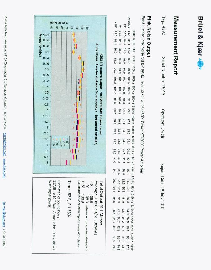
99 89