A semester of Experiments for ECE 225

Transcription

1 A semester of Experiments for ECE 225 Contents General Lab Instructions... 3 Notes on Experiment # ECE 225 Experiment #1 Introduction to the function generator and the oscilloscope... 5 Notes on Experiment # ECE 225 Experiment #2 Practice in DC and AC measurements using the oscilloscope Notes on Experiment # ECE 225 Experiment #3 Voltage, current, and resistance measurement Notes on Experiment # ECE 225 Experiment #4 Power, Voltage, Current, and Resistance Measurement Notes on Experiment # ECE 225 Experiment #5 Using The Scope To Graph Current Voltage (i v) Characteristics Notes on Experiment # ECE 225 Experiment #6 Analog Meters Notes on Experiment # ECE 225 Experiment #7 Kirchoff's current and voltage laws P age

2 Notes on Experiment # ECE 225 Experiment #8 Thevenin s Theorem Notes on Experiment # ECE 225 Experiment #9 Theorems of Linear Networks Notes on Experiment # Operational Amplifier Tutorial ECE 225 Experiment #10 Operational Amplifiers Notes on Experiment # ECE 225 Experiment #11 RC Circuits Notes on Experiment # ECE 225 Experiment #12 Phasors and Sinusoidal Analysis P age

3 General Lab Instructions The Lab Policy is here just to remind you of your responsibilities. Lab meets in room 3250 SEL. Be sure to find that room BEFORE your first lab meeting. You don't want to be late for your first (or any) lab session do you? Arrive on time for all lab sessions. You must attend the lab section in which you are registered. You can not make up a missed lab session! So, be sure to attend each lab session. REMEMBER: You must get a score of 65% or greater to pass lab. It is very important that you prepare in advance for every experiment. The Title page and the first four parts of your report (Purpose, Theory, Circuit Analysis, and Procedure) should be written up BEFORE you arrive to your lab session. You should also prepare data tables and bring graph paper when necessary. To insure that you get into the habit of doing the above, your lab instructor will be collecting your preliminary work at the beginning of your lab session. Up to four points will be deducted if this work is not prepared or is prepared poorly. This work will be returned to you while you are setting up the experiment. NOTE: No report writing (other than data recording) will be allowed until after you have completed the experiment. This will insure that you will have enough time to complete the experiment. If your preliminary work has also been done then you should easily finish your report before the lab session ends. Lab reports must be submitted by the end of the lab session. (DEFINE END OF LAB SESSION = XX:50, where XX:50 is the time your lab session officially ends according to the UIC TIMETABLE.) If your report is not complete then you must submit your incomplete report. If you prepare in advance you should always have enough time to complete your experiment and report by the end of the lab session. 3 P age

4 Notes on Experiment #1 Bring graph paper (cm cm is best) From this week on, be sure to print a copy of each experiment and bring it with you to lab. There will not be any experiment copies available in the lab. The purpose of this experiment is to get familiar with the function generator and the oscilloscope. During your lab session read very carefully and do everything just as described in the text. For each question that you encounter in the text, write down the question and then answer the question. There is very little calculation required. Please do draw the sketches required at the end of Section III. Experiment1 is a bit long and so you may not finish. That's OK. There will be no penalty if you do not finish. But do as much as you can. It will make the next experiment go easier for you. To prepare for this experiment: 1. Read the entire experiment. 2. Write down all the questions that are asked in the text of the experiment. 3. Prepare a title page, purpose paragraph (no theory or circuit analysis), and the questions (with space for the answers) in advance to coming to lab. 4. Also include, as an appendix to your lab report, the Multisim simulation that is due this week. Your report, which is due at the end of the lab session, will include the material above, the answers to the questions (which you will determine from performing the experiment), and a conclusion paragraph. 4 P age

5 ECE 225 Experiment #1 Introduction to the function generator and the oscilloscope Purpose: To familiarize yourself with the laboratory equipment Agilent 54622A Oscilloscope, Agilent 33120A 15MHz Function/Arbitrary Equipment: Waveform generator I. General Introduction 1. The function generator is a voltage source. It is most generally set so that the voltage at the output terminal is v(t) = B + Asinωt volts where a. B is the DC component of v(t) called the DC offset or just the offset b. Asinωt is the AC component of v(t). Note that the AC component is a periodic function of time. There are other periodic waveform shapes available from the function generator. The AC component has three parts: Shape (sin implies a sinusoidal shape); Amplitude (A is the zero-to-peak amplitude); Frequency (in this example the frequency would be radian frequency. But note that the function generator frequency must be set in Hertz (Hz)) Here are some useful terms: Radian frequency ω = 2πf where f is frequency in Hertz (i.e. cycles/second) Period T = 1/f = 2π / ω Zero-to-Peak Amplitude = A for a sinusoidal function Peak-to-Peak Amplitude = 2A for a sinusoidal function RMS Amplitude = A /(2) 1/2 = 0.707A for a sinusoidal function There are controls on the function generator that allow you to set each of the parts of v(t) (B, A, shape, frequency) very accurately. 5 P age

6 2. The oscilloscope is a voltmeter. You measure the voltage by observing the graphical image on the display. The parts of the voltage v(t) (B, A, shape, frequency) above can be determined very easily on the "scope." The scopes in your lab are digital "dual trace" oscilloscopes. They are capable of measuring two voltages simultaneously. Note that the scope has two sets of input terminals. Each input is called a channel. More about this later in the experiment. II. Learning to use the function generator 1. The function generator controls Take a look at the Agilent 33120A 15MHz Function/Arbitrary Waveform generator. Locate the sync and output terminals on the right hand side of the front panel. Note the special "Pomona plug" connector attached to each terminal. The function v(t) would be available at the output terminal. The voltage at the sync terminal is a special waveform that we will take a look at later in this experiment. Just to the left of the terminals are four arrow buttons. These are used to select menu options and to make incremental changes in various numerical quantities (frequency, amplitude, offset, etc.) So the arrow buttons are multi-purpose in nature. Which arrow button do think is used to select a peak-to-peak voltage setting? Which arrow button do you think is used to select mega-hertz frequency setting? Which button selects an RMS voltage setting. Just above the arrow button is a large dial knob. This dial knob can be used to set numerical quantities for frequency, amplitude, offset, etc. You can also use this dial knob to "fine tune" any quantity. Locate the three buttons under the Function/Modulation heading on the left side of the front panel with the sine wave, square wave, and triangle wave shapes. These buttons allow you to select the wave shape of the AC part of v(t). Just below these three buttons are buttons used to set the frequency, amplitude, and DC offset of v(t) The buttons described above are the features most frequently used for the experiments in this lab. Press the power button. Observe the display. Record what is written to the display exactly as you see it. Press the button with the triangle waveform. How does the display change. Press the square waveform button. How does the display change? Press the sine waveform button. 2. Setting the frequency 6 P age

7 Press the frequency button labeled Freq There are three methods to set numerical values. These methods apply to all function settings. i. Using the dial knob and left - right arrow buttons. Turn the dial and observe how the display changes. Note also that one of the digits is blinking off and on. Press the left arrow button. What happens? Press the right arrow button. What happens? Use the left and right arrow buttons to select the left most (most significant) digit as the blinking digit. Now turn the dial knob and set this digit to 7. Now press the right arrow key once to select the digit to the right. Again use the dial knob to set this digit to 7. Repeat this for the next two digits to the right. What is the value of the frequency displayed? ii. Using the arrow buttons The up and down arrow buttons can be used to increment and decrement digits in the display. Use the left and right arrow buttons to select the left most digit. Press the down arrow button. What happens? Press the up arrow button what happens? Use the up and down arrow keys to set this digit to 3. Use this method to set the three digits to the right to value 3. What is the value of the frequency now? iii. Using the Enter Number button Note that the twelve keys on the left and center of the panel have green numbers printed to the left of each key. Which key has the number 7? Which key has the +- symbol? Which key has the decimal point? You can use these keys for numerical input if you press the Enter Number key. Press the Enter Number key. Now enter the following key sequence: 6,., 3, 2, 4 Now press the ENTER button. What is the frequency displayed? You may change the units to MHz by pressing the MHz (up arrow button) instead of the ENTER button. Set the frequency to MHz iv. Practice Use each of the above methods to set these frequencies: 7 P age

8 8 P age 27.3 khz 351 Hz MHz khz What happens when you try to set the frequency to 20 MHz? Set the frequency back to 1 khz and go on to the next section 3. Setting the AC magnitude Press the Amplitude key Ampl and record exactly what appears on the display. To set the amplitude to 2 volts peak-to-peak. Press Enter Number a. Press 2 b. Press V pp (the up arrow button) Note that you have created the pure sinusoidal voltage v(t) = 1sin2000πt volts This has an RMS value of 1/(2) 1/2 = volts. We can set this value directly. c. Press Enter Number d. Press e. Press V rms (the down arrow button) Record exactly what appears in the display. What happens when you try to set the voltage to 12 volts peak-to-peak? What happens when you try to set the voltage to 0.03 volts peak-to-peak? Set the amplitude to 1 volt peak-to-peak and go on to the next section. 4. Setting the DC offset Press the offset button and record exactly what you see in the display. Now let's set the DC offset to 1.2 volts.. Press Enter Number a. Press 1.2

9 b. Press ENTER Reset the DC offset to zero. 5. Putting it altogether Note that the frequency given below in the argument of the sine function is in radians. You must convert the radian frequency to hertz (Hz, KHz, or MHz) to set the function generator properly. (Recall that w = 2πf so f = ω/2π) Note also that it is best to set the AC magnitude before setting the offset. (Recall that V pp = 2*A where A is the coefficient of the sine wave signal Asinωt volts.) Set the output voltage v(t) to: sin2000πt volts a sin500πt volts b sin7000πt volts 6. Learning to use the oscilloscope 0. The oscilloscope controls Take a look at the Agilent 54622A 100MHz Oscilloscope. Locate the two input terminals labeled 1 and 2. Note the special "Pomona plug" connector attached to each terminal. Just above these terminals are the "vertical" presentation controls. The small dial knobs with the up-down arrows along side them are the vertical position controls which allow you to move the image on the display up and down. The soft buttons labeled 1 and 2 allow you to access display menus for each channel. The larger dial knobs above the soft buttons are the vertical scale controls. The horizontal scale and position controls are at the very top of the front panel. The small dial knob with the left-right arrows below it is the horizontal position control which allow you to move the image on the display left and right. Locate the controls labeled Quick Meas and Auto scale. These are the buttons you will use most often when measuring voltages with the scope. Locate the Run/Stop and Single controls. They are used to control the digital "sampling" of the voltages being measured. They will help you to get a stable image on the display. Whenever the image that appears on the display is unstable, just press Run/Stop to stabilize the image. 9 P age

10 1. Measuring voltages with the scope Connect the function generator terminal labeled output to the channel 1 input terminal using the red and black cables available in the lab. Now press the power button (at the lower right corner of the display) to turn on the scope. An information page is displayed on the screen for about 15 seconds. Set the function generator to the following voltage: 1 + 2sin2000πt volts (Be sure to set the AC part first.) Press Auto scale There should be a sinusoidal image in the center of the display. Take a look along the edges of the display. Information about the location of the horizontal and vertical axis (small black arrows with right angle shafts), the vertical scale (in the upper left corner) as well as other values has been displayed along the edges of the display. Of course you also see the voltage image at the center of the display. To what value has the vertical scale been set? Use the vertical scale to determine the peak-to-peak voltage of the sine wave image that appears in the display. Is the value of the peak-topeak voltage what you expected? If the value is not what you expect, don't worry, we will learn to fix this a bit later in the experiment. Play with the small dial knobs with the up-down arrows along side them (the vertical position controls) to move the image on the display up and down. Play with the small dial knob with the left-right arrows below it (the horizontal position control) to move the image on the display left and right. You can use the position controls to move an image to a location on the display that may make it easier for you to make more accurate visual measurements. 2. The channel 1 menu i. Press the soft 1 button one time. Notice the menu options at the bottom of the display. ii. Select the probe option by pressing the key below the word probe. Now turn the dial knob next to the circular arrow. What happens? Set the probe setting to 1.0:1 This will insure that the scope is correctly calibrated for the probes (which in this case are just the wire cables.) 10 P age

11 You should try to remember to set the probe option to 1.0:1 every time you use the scope in this lab. iii. Note that the coupling option is set to DC. This means the image on the display contains both the DC and AC components of the voltage signal. Select this option and change the coupling to AC. How has the image on the display changed? In this setting only the AC component of the signal is displayed. The DC has been removed. Change the coupling back to DC. iv. Select the invert option. This changes the sign of the signal. What happened to the image on the display? To get the signal back on the display use the position control dial knob just below the soft 1 button Adjust this control until the horizontal axis is at the second grid line from the top of the display. You may now need to press Run/Stop a couple of times to get a "clean" image. Select the invert option again and reposition the image so that the horizontal axis is at the second grid line from the bottom. v. Turn the vertical scale dial knob (just above the soft 1 button) Note that the scale value is changing (upper left corner edge of the display) Set the scale to 1.0V/ How does the image in the display change? Now set the scale to 2.0V/ and then to 200mV/ Note how the image changes as the scale changes. Remember, if the image is unstable press the Run/Stopbutton a few times. Note that the "best" scale is the scale that makes the image as large as possible but no part of the image goes beyond the top and bottom of the display. Find the "best" scale for the image. What is the scale setting for the "best" image? vi. Press the Quick Measure button The scope will now do all of your measurement for you! Press each of the following menu options and record the values given on the display: (Use the arrow option to access more options) 1. Frequency 2. Peak-Peak 3. RMS 4. Maximum 5. Minimum 6. Average (is the DC value of the signal) Have you noticed that the image on the display is twice as big as it should be. Have you noticed that the measured 11 P age

12 values of the peak-to-peak voltage and the average value are twice as big as they should be? The problem is in the function generator. Here is the fix. On the function generator: 7. Press Shift (the blue button) 8. Press Menu 9. Repeatedly press Right Arrow until the display shows D: SYS MENU 10. Press Down Arrow two times so that the display shows 50 Ohms 11. Press Right Arrow one time so that the display shows High Z 12. Press Enter Now reset the function generator for 1 + 2sin2000pit Go back to the scope and measure the peak-to-peak and average values. They should now be correct. Please note: The scope will always give the correct measurement. When in doubt, use the scope measurement and not the function generator display to determine the actual voltage at the output of the function generator. vii. Measuring two signals at one time. Here will will be displaying two very different images ( a sine wave from the output connection of the function generator and the SYNC signal - a pulse wave from the SYNC connection of the function generator) at the same time. Set the function generator to: 0 + 2sin4000πt With the output terminal of the function generator still connected to the channel 1 input of the scope, connect a set of cables from the SYNC terminal to the channel 2 input of the scope. Now press Auto scale. There should be two images on the scope. Make a sketch of all that is on the scope display. You can turn off either channel by pressing the channel soft button two times. Turn off channel 1 now. 12 P age

13 Use the channel 2 vertical position control knob to adjust the position of the channel 2 horizontal axis (remember the black arrow with the right angle shaft?) so that it is at the center of the display. Turn on channel 1 and turn off channel 2. Move the channel one axis to the center of the display. Turn channel 2 back on. The two images overlap. Sketch what is on the display. Let's do some math! Press the math soft button and select the menu option 1-2. There are three images on the display now. Turn off channels 1 and 2 The remaining image is the difference between the voltages input to the two channel. To set the vertical scale of the math mode image press the settings option (accessed by pressing the math soft button once) and then turn the indicted control knob so that the vertical scale is 2.00V/ Sketch this image. Repeat the above procedures using the triangle waveform and then the square waveform from the function generator. You should now be familiar with the operation of the function generator and the oscilloscope. Bring this experiment with you each time you come to the lab. It will be a useful reference for future experiments. 13 P age

14 Notes on Experiment #2 The purpose of this experiment is to get some practice measuring voltage using the oscilloscope. You will be practicing direct and differential measuring techniques. You will also learn that under certain conditions the scope can give what appears to be wrong values if connected to the circuit incorrectly. You will also learn how to construct a circuit on the "breadboard" and how to set the DC and AC power supplies. Your circuit analysis will lead you to the expected values of the various voltages indicated in the circuit diagram. You will then measure the voltages and compare that data to your calculated values from your circuit analysis. (i.e. do some error analysis) To find a voltage in this circuit first use Ohm's law to find the total current. Then find the individual voltages using Ohm's law again. So, I = Vs/(R1 + R2 + R3) V1 = I*R1 V2 = I*R2 V3 = I*R3 V4 = I*(R1 + R2) V5 = I*(R2 + R3) Note if Vs is a pure DC voltage then all of the above voltages will also be pure DC (i.e. constant values.) If Vs is an AC voltage then all of the voltages will also be AC. DC + AC Example (NOTE: THESE ARE NOT THE VALUES FROM THE EXPERIMENT) Vs = sin(100t) volts R1 = 10K R2 = 15K R3 = 25K I = ( sin(100t))/(10K + 15K + 25K) = sin(100t) ma. So, V2 = sin(100t) ma.*15k = sin(100t) volts 14 P age

15 Hope this helps you with your preparation for experiment #2. Please note that calculations like the above are the work that you must do (for each section of the experiment) as your preliminary work. Also, make a list all of the questions you find in the text of the experiment. These questions will require answers that must be included in your write-up. Experiment 2 takes a lot of time. Prepare as much of your report as possible BEFORE going to lab. 15 P age

16 ECE 225 Experiment #2 Practice in DC and AC measurements using the oscilloscope Be sure to bring a copy of this experiment and a copy of experiment 1 (as a reference for equipment operation) to the lab this week. Purpose: To familiarize yourself with the DC voltage supply, and to practice using the oscilloscope DC and AC measurements. Equipment: Agilent 54622A Oscilloscope, Agilent 33120A 15MHz Function/Arbitrary Waveform Generator, Agilent E3631A Triple Output DC Power Supply, Universal Breadbox I. The Agilent E3631A Triple Output DC Power Supply 16 P age The Agilent E3631A has three power supplies, a +6 V supply capable of delivering 5A, and two supplies of +25 and -25 V capable of delivering 1A each. The (ground) output is the reference ground and is connected to the ground of the building. Under normal use (for safety reasons) it is important to connect the COM (common) terminal of the +25 V supplies, and the (-) terminal of the +6 V supply to the (ground) reference. 1. Looking now at the control keys: The Output ON/OFF key turns the output ON or OFF. 2. To Set the Output Voltage: a. Press the +6, +25, -25 keys to select the power supply to be set. b. Press Voltage/Current key so that the Volt Display is active. c. Use the circular control knob to set the output voltage. Use the arrow keys for selecting the resolution. 3. To Set the Maximum Output Current: a. The Display Limit key lets you select the maximum current that the power supply can deliver (up to 5A for the 6V and 1A for the +25V supplies). This is basically your current protection feature. b. Press Voltage/Current the key so that the Current Display is active. c. Use the circular control knob and the resolution keys to set this limit (if needed). d. Practice. Set each output to 3.7 volts with current limit at amps.

17 4. To Read the Output Voltage or Output Current: a. The Voltage/Current key also shows the output voltage and the output current of the power supply. b. To measure the output current of the supply, make sure that the Display Limit key is not active. II. The Oscilloscope As A DC Voltmeter: Direct Measurement Warm up the oscilloscope, function generator, and the DC supply. Set up the circuit in Figure 1 below using the + and COM terminal of the +25 volt output terminal of the DC supply for V S. So, the + side of V S is the + side of the +25 terminals and the - side of V S is the COM side of the +25 terminals. Set V S to 8 Volts. Set the current limit to Amps. Let R 1 = 20K R 2 = 33K R 3 = 47K Figure 1. Calculate V 1, V 2, V 3, V 4, and V 5. Measure each of the voltages using channel 1 of the oscilloscope. (Press Auto Scale for easy scope measurements.) Note that these voltages are all DC values. So, be sure that the channel 1 coupling is set to DC. You should see only a straight horizontal line on the display of the scope. This line will be above the horizontal axis for channel 1. The distance above the axis times the vertical scale is the DC value of the voltage. If the image is very "fuzzy" try setting the channel 1 vertical scale (dial just above the 1 button) to a larger value like 2.00V/ or press the Single button. Record your measurements. Repeat these measurements using channel 2. Record these measurements. Do channels 1 and 2 give exactly the same measurements? Note that you could very accurately 17 P age

18 measure the voltages using Quick Measure and the average value measurement option. Compare your measured values to your calculated values from your preliminary report and determine the percent error using: %ERR = [(measured value - calculate value)/(calculated value)] X 100 III. The Oscilloscope As A DC Voltmeter: Differential Measurement Next we will be measure two voltages simultaneously and have the math mode feature of the scope display their difference. Connect the negative (black) terminals of both channel 1 and 2 to the COM terminal of the DC supply. (Note that COM is NOT the ground ( ) terminal.) To measure V 3 connect the positive (red) terminal of channel 1 to the + polarity node of V 3 and connect the positive (red) terminal of channel 2 to the - polarity node of V 3. Now press the Math button and select option 1-2. Turn off channels 1 and 2 (press the channel 1 and 2 buttons twice each.) The image on the display is now V 3. Prove that this must be true using Kirchoff's voltage law. Remember that you are able to adjust the vertical scale of the math mode image. (See experiment 1.) Adjust the math mode vertical scale so that you may get an accurate measurement. You will notice that there is no horizontal axis marker at the left edge of the display. You can create a horizontal axis using the cursor option. Press the cursor button. Now choose the X Y button to get the Y (horizontal) cursors. Select the Y 1 button and then turn the indicated dial knob to set the Y 1 cursor to read 0.00 volts. The position of this cursor is now the location of the horizontal axis. You can now measure the value of the voltage with respect to the location of the Y 1 cursor. To reposition the horizontal axis press the math button one time and select the settings option. Now select the offset option and then turn the indicated dial. Adjusting the offset will allow you to position the horizontal axis (the Y 1 cursor.) Use this method to move the axis down to the first line above the bottom of the display. Now select the scale option and adjust the scale to 2.00V/. You may need to reposition the axis again as explained above. You should now be able to get a very accurate measurement. Use the differential measuring method to measure all of the voltages in Figure 1 including V S. Record your measurement. Compare these measurements to your calculated values. The following section was omitted from experiment 2. This should explain your data. IV. The Problem With Ground 18 P age Leave the circuit set up as it is. Get another black cable and use it to connect the ground terminal ( ) of the DC supply to the COM terminal of the +25 volt output of the DC supply. Doing this will have no effect on the circuit. However, this will cause a problem when measuring voltages with the scope. Repeat all of the measurements of the previous two sections. How has the accuracy of your measurements been affected.

19 The negative side of the scope is connected to earth ground through the chassis of the scope. So whenever a voltage measurement is made with the scope, the measurement is being made with respect to earth ground. There is no getting around that fact! Therefore if a circuit under investigation has a node connected to earth ground, then the negative side of the scope (the BLACK lead) must be connected to that node. If the negative side of the scope is connected elsewhere, a "short circuit" will be created and all voltage (and current) values in the circuit will change! A source, instrument, or circuit that has no connection to earth ground is said to be "floating." When the ground terminal of the DC supply is not being used, the supply is floating, as it was in the initial part of this experiment. For a circuit that is floating the negative side of the scope may be connected to any node of the circuit without upsetting any voltage or current values. A short circuit can cause a disaster to a circuit and its components. So, if you are not sure about the ground situation for a circuit then use the differential measuring technique when measuring voltages with the scope. V. Using The Scope For Direct And Differential AC Measurement Remove the Agilent DC supply from the circuit and replace it with the Agilent function generator as the voltage source V S. Be sure to use the black terminal of the function generator as the - side of V S. Set V S = 5 cos(3000pit) volts. (Don't forget to set the function generator into the HIGH Z output mode. (See experiment 1.) Be sure that the DC offset is set to zero. Calculate V 1 through V 5. Using the differential measurement technique, measure and record V peak-to-peak for all of the voltages. Repeat all of the measurements using the direct measurement technique Calculate the %ERR of each of the measured voltages with respect to the calculated values. 19 P age

20 Notes on Experiment #3 This week you learn to measure voltage, current, and resistance with the digital multimeter (DMM) You must practice measuring each of these quantities (especially current) as much as you can. When we give the lab exam (later in the term) each of you will individually be required to demonstrate these measuring techniques. Practice makes perfect. :) Be sure to calculate all of the expected voltages and currents of each circuit BEFORE you come to lab. 20 P age

21 ECE 225 Experiment #3 Voltage, current, and resistance measurement Purpose: To measure V, I, and R with a Digital Multimeter (DMM.) We also verify Kirchoff's Laws. Equipment: Agilent 34401A Digital Multimeter (DMM), Agilent 33120A 15MHz Function/Arbitrary Waveform Generator, Agilent E3631A Triple Output DC Power Supply, Universal Breadbox I. General Introduction to the DMM 1. Voltage and Current The voltages and currents measured in this lab generally take on the form v(t) = B + Asinwt volts where a. B is the DC component of v(t) called the DC offset or just offset b. Asinwt is the AC component of v(t). Note that the AC component is a periodic function of time. The AC component has three parts: Shape (sin implies a sinusoidal shape); Amplitude (A is the zeroto-peak amplitude); Frequency (in this example the frequency would be radian frequency. Recall these useful terms: Radian frequency w = 2pif where f is frequency in Hertz (i.e. cycles/second) Period T = 1/f = 2pi /w Zero-to-Peak Amplitude = A for a sinusoidal function Peak-to-Peak Amplitude = 2A for a sinusoidal function RMS Amplitude = A /2 1/2 for a sinusoidal function 21 P age

22 There are controls on the DMM that allow you to measure each of the parts of v(t) (B, A RMS, and frequency) very accurately. Note that each key has two (or more) options. To select the function printed on a key just press the key. To select the function printed just above the key you must first press the blue Shift key and then the function key. For example, if you wish to measure DC current then you must press the Shift key and then the DC V key to put the DMM into DC I (DC current) measuring mode. Note that you may only measure one quantity at a time. You must select either the DC V or AC V key to measure DC or AC voltages respectively. 2. Range Setting The are two range modes: Auto ranging (the default mode) and Manual ranging. You may toggle between the two ranges by pressing the Auto/Man key. Pressing an arrow key puts the DMM into manual ranging mode and allows you to select a higher (arrow up) or lower (arrow down) range. If a range is to low for a value being measured then the meter goes into an overload condition indicated by OVLD printed to the display. To get out of overload simple select a higher range or select auto ranging. The most accurate rage is the lowest possible range that does not put the meter into an overload state. 3. Terminals For voltage and resistance measurements use the two upper right hand terminals just below the Omega V diode symbols. HI is the positive (+) terminal and LO is the negative (-) terminal for the voltage measurement. Use the two lower right hand terminals I and LO for current measurement. The I terminal is the positive terminal for the current measurement. The most common mistake made in the lab will be forgetting to move the positive connection from HI to I when going from a voltage measurement to a current measurement. 4. How to measure current, voltage, and resistance Your Teaching Assistant will explain to you how to use DMM to measure currents, voltages, and resistances. However, note the following: a. To measure voltages, you only need to attach the leads of the DMM to two points of the circuit, select the DC V or AC V function, and select a meter range. The meter reading gives the voltage of the point connected to the HI terminal (use a red cable) with respect to the point connected to the LO terminal (use a black cable.) Voltage readings are the easiest type to take. 22 P age

23 b. To measure currents, you must break the circuit at the point where the unknown current flows, and re-route the current through the meter, entering at the I terminal (use a red cable) and leaving at the LO terminal (use a black cable.) Then you must select the DC I or AC I function, and select the appropriate range. c. To measure resistance, you must disconnect at least one side of the resistor from the circuit before attaching it to the DMM terminals or leads. If you leave the resistor in the circuit and try to measure it in place, you are likely to get bizarre results. This is because the DMM sends current through the resistor to perform the measurement, and it assumes that the current flows only through that single resistor. If the resistor is still connected to the circuit, the current from the DMM might go through other paths, with unpredictable results. Press the key labeled Omega 2W. 2W stands for the "two wire" measurement. Now select a range. II. Current, Voltage, and Resistance Set up the circuit in Figure 1 using the DC supply for V S and a 3.3K resistor for R. Adjust the DC voltage supply until the DMM, used as an ammeter, shows that the current is 1.00 ma. Then remove the DMM from the circuit (don't forget to reconnect the bottom of R to V S ) and use it, now as a voltmeter, to measure the voltage across the resistor. Last, disconnect the resistor from the circuit and use the DMM to measure its resistance. Do the three readings verify Ohm's Law? Record the measurements and the percent error observed between R measured directly, and R calculated by R = V/I. Compare both of these values with the value of the resistor read from its color code (the so-called "nominal" value) and see whether or not the value is within the stated percentage tolerance. Figure P age

24 III. Measuring Voltage Set up the circuit in Figure 2 with R 1 = 20K R 2 = 33K R 3 = 47K V 6 = 8 Volts (use the COM terminals of the DC supply with the current limit set to 100mA. Remember that you are setting the maximum current that the generator will be able to deliver and not the actual value that is being delivered - you will measure that value.) Figure 2. Measure all six voltages with the voltmeter (the DMM set on the DC voltage setting.) Using your DATA, make a table indicating the percent inaccuracy, according to your measurements (i.e. your DATA), in these three Kirchoff voltage law relationships: V 1 + V 2 = V 4 V 2 + V 3 = V 5 V 1 + V 2 + V 3 = V 6 Do the data values on the left sum to the data on the right? That is the inaccuracy error that you are checking. Measure the three resistors with the DMM and make a table indicating the percent inaccuracy, according to your measurements, in the relationships V 3 /R 3 = V 2 /R 2 = V 1 /R 1 = I 24 P age

25 We have not measured I yet. But each of the above ratios should equal the same value of I since the same I is flowing in all three resistors. Are the currents the same? Now remove the DC supply from the circuit and insert the function generator as V S. Set V S = 4sin(3000pit) volts. The DC offset should be set to zero. Now repeat the above experiment making AC voltage measurements. IV. Measuring Currents There are two ways to measure currents: (1) directly, using an ammeter, and (2) indirectly, using a voltmeter (or a scope) to measure the voltage across a resistor and then calculating the current by use of Ohm's Law. The second method, of course, is only accurate if you have an accurate value for the resistor. Set up the circuit in Figure 3 with R 1 = 20K R 2 = 33K R 3 = 47K V S = 8 Volts (use the COM terminals of the DC supply with the current limit set to 100mA.) Figure 3. Measure the indicated currents directly by inserting the ammeter (the DMM set on the DC I setting) into the circuit at the locations indicated by "I 1 ", "I 2 ", etc. Record your observations in a table and indicate the percent inaccuracy, according to your measurements, in the Kirchoff's current law relationships I 1 + I 2 = I 4 I 3 + I 4 = I 5 25 P age

26 Now measure the indicated currents indirectly (by measuring the voltages, measuring the resistances, and using Ohm's law) and repeat the above calculations of inaccuracy. We will not do AC current measurements in this experiment. 26 P age

27 Notes on Experiment #4 Use only Ohm's Law, Voltage Division, Current Division and the Power equation to do your circuit analysis. Do part I as is. In part II you will be measuring and recording the voltages with both the DMM and the scope. So set up your data tables accordingly. For the circuit analysis in part I you MUST USE VOLTAGE DIVISION to find every voltage value. For the voltage Vi across a single resistor Ri we have: Vi = [Ri/(R1 + R2 + R3 +R4)]*Vs If you need the voltage across two adjacent resistors, say R1 and R2, then let Ri = R1 + R2 in the above formula and you have it! For the circuit analysis in part III you MUST USE CURRENT DIVISION to find every current value. In this case you MUST find Is first. Is = Vs*(1/R1 + 1/R2 + 1/R3 + 1/R4) = Vs/Req, Where Req = R1 R2 R3 R4 then For the current Ii in a single resistor Ri we have: Ii = [Gi/(G1 + G2 + G3 + G4)]*Is, Where G = 1/R (conductance) For the current in two resistors, say R1 and R2, then Gi = G1 + G2 27 P age

28 ECE 225 Experiment #4 Power, Voltage, Current, and Resistance Measurement Purpose: To measure V, I, and R with a Digital Multimeter (DMM) and the V with the oscilloscope; verify voltage and current division rules; investigate the effect of power dissipated by a resistor Equipment: Agilent 54622A Oscilloscope, Agilent 34401A Digital Multimeter (DMM), Agilent 33120A 15MHz Function/Arbitrary Waveform Generator, Agilent E3631A Triple Output DC Power Supply, Universal Breadbox I. Power Accurately measure the resistance of a 27-ohm, 1/4 watt resistor. If the value is more than 5% in error ask your lab instructor for a replacement resistor. Calculate the DC voltage which results in 1/2 watt of power dissipation in the resistor, and set the DC supply to that value. Use the + and - terminals of the 6 volt output. Set the current limit to 200 ma. Attach cables from breadbox directly to the + and - terminals of the DC voltage supply. Use hookup wire to connect the resistor to the cables. Wait a few minutes and feel the resistor. Comment. Disconnect the resistor from the DC supply and measure the resistor's value and see if the value has changed as a result of the abuse. Now repeat the experiment with the DC supply set for a power dissipation of 1 watt (four times the rated amount). Don't burn yourself! Be sure to measure the resistor again before you start the 1 watt trial. II. Voltage Division For the next two parts you will need accurate values of the resistors in order to verify the voltage division and current division shortcuts. Measure these values accurately if you have not already done so. Set up the circuit in Figure 1. using the DC supply as V S. Set V S to 10 volts. Then by measuring V 1, V 2, V 3, V 4, V 12, V 123, and V S with the DMM, verify the voltage division rule for each of these voltages. Present your results (measured values vs. values calculated on the basis of the voltage division rule, using the accurately measured R values) in the form of a table. Next, replace the DC supply with the function generator, set it for a waveform 4sin(4000pit) volts (be sure the DC offset is zero), and repeat. Next, repeat all of the above measuring the voltages with the oscilloscope. 28 P age

29 R 1 = 1.0K R 2 = 3.3K R 3 = 2.0K R 4 = 4.7K Figure 1. III. Current Division Verify the current division rule, in a manner similar to your verification of the voltage division rule above, for the circuit in Figure 2. Let V S be 10 volts DC. Measure the currents using the DMM. No need to use the scope. The scope is a voltmeter. NOTE: WE WILL NOT DO AC CURRENT MEASUREMENT. THE AC CURRENTS ARE TOO SMALL TO BE MEASURED BY THE DMM IN THIS LAB. R 1 = 1.0K R 2 = 3.3K R 1 = 2.0K R 1 = 4.7K Figure P age

30 Notes on Experiment #5 This week we will do experiment 5 AS IS. Your data will be the graphical images on the display of the scope. So, BRING GRAPH PAPER! cm X cm is best since that is the actual scale of the scope display. You will be sketching the current/voltage characteristics of several elements and simple networks. Since many of these i/v curves are non-linear the term NL is used as the test element (or network) general name. When NL = a resistor then of course the i/v curves follow the linear relation of Ohm's law. So, i = (1/R)v The equation of a line! So you should see a line on the display that has a slope = 1/R and a i-intercept at (0,0) When NL is a series combination of a battery Vb and a resistor R then it is easy to show that: i = (1/R)v - (1/R)Vb A line again! The slope is still 1/R but the i-intercept is -(1/R)Vb Show that this is true by doing the circuit analysis. No other circuit analysis is required. Read and know the setup of this experiment and Have fun! 30 P age

31 ECE 225 Experiment #5 Using The Scope To Graph Current Voltage (i v) Characteristics Purpose: to become skilled at obtaining v-i characteristics of circuits and devices. Equipment: Agilent 54622A Oscilloscope, Agilent 33120A 15MHz Function/Arbitrary Waveform Generator, Universal Breadbox I. Introduction One way to measure the i-v characteristic of a device is to attach a DC voltage source to it, measure the voltage and current, thus obtaining one i-v combination (one point on a graph), and then repeat for many combinations. It is much more efficient to get the scope and the function generator to display the i-v characteristic directly on the screen of the scope. To do so the technique is as follows: a. Press the Main/Delayed key and then choose the XY option. This puts the scope into XY mode. b. Apply the voltage "v" to the CH1 or "X" input terminals of the scope, so that the horizontal axis of the scope can be interpreted as "v"; c. Apply a voltage proportional to "i" to the CH2 or "Y" input terminals of the scope, so that the vertical beam deflection is proportional to "i". This sets up an "i" vertical axis on the scope; d. Use an external time-varying source to cause "v" and "i" to change through a whole range of values, thus tracing out the i-v curve, and record the trace on the scope. This is exactly what will be done in this experiment. The circuit is shown below. Note that the voltage across the 1K resistor is proportional to the current "i" through the device in question, and its resistance is chosen to be 1K so that this voltage will be 1 volt when the device current is 1 ma, making the conversion to current units easy. It is also important that both CH1 and CH2 be set to DC. Explain why. 31 P age

32 The Circuit Setup Recall that the black terminal of the scope is the "ground" connection on the scope. In this technique the voltage applied to the vertical input is -Ri, so that the display will be the shape of the i-v characteristic, but upside down. Fortunately by using the invert option for CH2, the vertical ("-Ri") component can be inverted so as to be correctly oriented. Then vertical deflection = i in ma, and horizontal deflection = v in volts. To cause the device to experience a variety of i-v combinations, so as to trace out the characteristic curve, it is convenient to use the signal generator set to a triangle function. Different sections of the i-v curve can be viewed by changing the DC offset and the amplitude of the triangle. II. i-v Curve Of A Resistor 32 P age Set up the circuit with NL = a 2.7K resistor, which is of course a linear device and should result in a linear i-v characteristic curve, through the origin and with a slope equal to 1/R. Position the appropriate axis of both CH1 and CH2 to the center of the scope, which becomes the origin of the i-v graph. Set the frequency of the signal generator to 60Hz. Display and record the i-v curve (as much of it as you can get with maximum signal amplitude and maximal variations of the DC offset). Be sure to record this graph in units of Volts (horizontally) and milliamps (vertically). All graphs in this course should be labeled in electrical units such as

33 these. Compare the measured i-v graph with the theoretical expectation. If the 1 K resistor in the circuit is significantly different from 1000 ohms you may have to insert a correction factor for that, or you might try "building" a resistor which measures exactly 1000 ohms. Turn down the generator frequency to 1 Hz so you can see just what is happening here - a tracing out of a lot of individual i-v combinations, so fast at 60Hz that they blend into an apparently solid curve. Incidentally you can do a little experiment here about human perception. Experiment to determine the lowest frequency (in the neighborhood of Hz) where the scope trace appears to you to stop flickering and look "solid." Movies and TV must refresh their images at this frequency or faster in order to convey the impression of smooth movement. III. i-v Curves Of Other Elements Once you understand part II, go on to record the characteristics of other devices, as given in the figures below. The first one is of course a linear circuit and should give a linear i-v curve. It is constructed from the DC voltage source in series with a plain resistor. The other devices are not covered in this course but they have interesting i-v curves. You don't need to know anything about the diodes in order to graph their i-v characteristics! Some devices to try: Thevenin Equivalent Circuit 33 P age

34 Silicon Diode #1N4004 Zener Diode #1N4735 You may need to position the graph to the right so that you can see the details on the left. Try using some negative DC offset if the curve does not break in a downward direction on the left side. Leaky Diode Simulation Leaky Zener Simulation 34 P age

35 35 P age Note: diode polarity (direction) is indicated by a ring, as follows:

36 Notes on Experiment #6 We will do experiment #6 AS IS. Follow the instructions as given. Analog Meters When attaching a meter to a circuit to make a measurement we would hope that the presence of the meter does not cause voltage and current values in the circuit to change. Analog meters, in order to operate, generally borrow energy from the circuit to which they are attached. This is called "loading the circuit." If the meter uses a very small amount of energy and does not cause voltages or currents to change then we say the meter is a "light load." If the meter draws a great deal of energy and current and voltage values in the circuit change dramatically then then meter is "loading down the circuit" or is "a heavy load." The Simpson multi-meter is an analog meter and will load a circuit when making a measurement. The DMM is almost an "ideal meter" and as such will be an extremely light load on a circuit. (There are cases when the DMM could load down a circuit however.) We will be using the DMM to observe the loading effect of the Simpson meter on a circuit. Current Meters All current meters can be modeled as a resistor R m. An ideal current meter has R m =0. A practical current meter has R m equal to "a very small resistance." The circuit in Figure_1 has a current meter in series with a voltage source and a resistor. The current in the circuit without the meter is I = V S /R If the meter is "in circuit" then the current becomes I = V S /(R + R m ) which is clearly a lower value than the original current. You will notice that this new current will actually be the current that the meter displays! 36 P age

37 Figure_1 Voltage Meters All voltage meters can be modeled as a resistor R m. An ideal voltage meter has R m =infinite resistance. A practical voltage meter has R m equal to "a very large resistance." The circuit in Figure_2 has a voltage meter in parallel with a resistor. The voltage V 2 in the circuit without the meter is (by voltage division) V 2 = [R 2 /(R 2 + R 1 )] * V S If the meter is "in circuit" then the voltage becomes V 2 = [{R 2 (R m } /({R 2 (R m } + R 1 )] * V S which is clearly a lower value than the original voltage. You will notice that this new voltage will actually be the voltage that the meter displays! 37 P age Figure_2 The internal resistance R m of the Simpson meter as a current meter is not available. If there is time, see if you can calculate it using your data from part 1 of the experiment. The internal resistance R m of the Simpson meter as a voltage meter is 20K X the scale setting. So, if the scale is on the 10 volt setting then R m = 20K X 10 = 200K On the 2.5 volt setting R m = 20K X 2.5 = 50K

38 Note that this is the scale setting used here and not the voltage value measured at this setting. For your circuit analysis in part 2. Calculate V 1 and V 2 with no meter and then again with the meter attached appropriately. Consult your lab manual for available voltage scales on the Simpson meter. Choose an appropriate scale for each measurement. Have fun. 38 P age

39 ECE 225 Experiment #6 Analog Meters Purpose: To illustrate use and pitfalls of analog meters Equipment: Agilent 34401A Digital Multimeter (DMM), Agilent E3631A Triple Output DC Power Supply, Universal Breadbox, Simpson Multipurpose Analog Meter I. Using an analog meter to measure current, voltage, and resistance CAUTION: with the Simpson meter, as with all analog meters, care must be taken to put the meter in the circuit with the proper polarity and on the proper range, or the meter can easily be damaged. Current must flow into the meter terminal which on analog meters such as this is usually labeled "+" or "V-A" or some such thing and is often colored red, and out of the terminal which is usually labeled "COM" or "GROUND" or "-", etc. and is often colored black. Ammeters should always be set initially to the least sensitive scale (labeled with the largest values of current) and then turned to more sensitive ranges until a good needle deflection is obtained. Similar precautions hold when using the Simpson as a voltmeter; polarity must be observed and you should start on the least sensitive scale, then switch to more sensitive ranges to get a good reading. These precautions are largely unnecessary for our digital meters multimeter (DMM), which if used wrong merely announces that fact by an overload indication. Taking these precautions, set up the circuit below. Throughout this part, leave the DMM in the circuit, operating as a current meter. Figure P age

40 Put the Simpson in the circuit as a current meter (in series with the DMM) and adjust the DC voltage supply until the current is 1 ma. Do the DMM and the Simpson agree? Then remove the Simpson from the circuit. Does the current (as measured by the DMM) change as a result of removing the Simpson? Now use the Simpson as a voltmeter to measure the voltage across the resistor. Pay close attention to the current (measured on the DMM): does the current change when the Simpson is attached to measure the voltage? Last, disconnect the resistor from the circuit and use the Simpson to measure its resistance. Do the readings of V, I, and R verify Ohm's Law? Record the measurements and the percent error observed in V = I R, with readings taken on the Simpson. Measure the same three quantities with the DMM and calculate the error in V = I*R again. Comment on your observations. II. Meter "loading" of a circuit A meter is said to "load" a circuit if attaching it changes the voltages or currents in the circuit being measured. In principle this loading should be zero. Set up the circuit below. Attach the DMM to measure V 1. Figure 2. Leaving the DMM attached, connect the Simpson to measure V 1 also. Does the addition of the Simpson affect the circuit? Record your observations. The degree of loading by the Simpson can be calculated. Its effect on the circuit is the same as if a resistor were attached, with a value of "20,000 ohms per volt" where the "volt" refers to the range used. For example, on the 10 volt scale it affects the circuit like connecting a resistor of 200K (= 20K ohms/volt x 10 volt scale.) Calculate the expected loading, that is, how much you would expect V 1 to change when the Simpson is attached. Compare this with your observations. Now repeat this experiment for V 2. Explain why the loading is less in this case. 40 P age

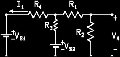
41 Notes on Experiment #7 Prepare for this experiment! During this experiment you will be building the most elaborate circuit of the term. (See Figure 1. below for circuit diagram and values.) You will also be measuring voltages and currents using all of the techniques we've learned this term. This will be great practice for the lab exam which will be later in the term. If you come to lab prepared you will finish early. If you do not prepare for this experiment you will not finish on time. Measure the Resistors First! The resistors must be accurate in this experiment. Discard any with an error greater than 5%. Ask your lab instructor for a replacement. Procedure We will do this experiment twice. The first time through we will use two pure DC sources. The second time through we will use one pure DC source and the function generator set to have pure DC. For each case above we will measure and record all voltages using: The DMM and The Oscilloscope. We will also directly measure and record the current in each element using the DMM. (That means each resistor and each source.) Set up appropriate data tables for the expected data. You will then compare this data to the calculated values from your circuit analysis and do error analysis. Circuit Analysis Use mesh analysis to determine the mesh currents. Then calculate each element current (including resistors and sources.) Now use Ohm's law to calculate each resistor voltage. You will be doing this twice!. First time: Use the dual DC supply for the two pure DC sources. R S = 0 Ohms, 41 P age

42 V S1 = 10 Volts DC, and V S2 = 6 Volts DC. Second time: Use the function generator for V S1 and one side of the dual DC supply for V S2. YOU MUST SET THE SOURCES BEFORE YOU CONNECT THEM TO THE CIRCUIT. WHY? R S = 50 Ohms (NOT K OHMS), V S1 = 10cos(2000(pi)t) Volts (AC), and V S2 = 6 Volts DC. 470 Ω 1K Ω 680 Ω 100 Ω Figure 1. Have fun. 42 P age

43 ECE 225 Experiment #7 Kirchoff's current and voltage laws Purpose: To verify Kirchoff's laws experimentally Equipment: Agilent 34401A Digital Multimeter (DMM), Agilent E3631A Triple Output DC Power Supply, Universal Breadbox I. Introduction If a branch of a circuit contains a resistor, the best way to measure the current in that branch is to measure the voltage across the resistor and divide by R. However this gives a value which is only as accurate as the value of R. Consequently, start this investigation by accurately measuring the values of all resistors which will be used. Of course if a branch of a circuit contains no resistors, the current in that branch must be measured directly with a milliammeter (or else deduced by Kirchoff's current law from other known currents.) II. Verifying KCL, KVL, and power balance for a linear circuit (DC) Set up the circuit in Figure 1. Use the +25 volt output for V S1 (set to 10 volts) and the 6 volt output for V S2 (set to 6 volts.) Set the current limits to 100mA. Use the DMM for measurements. 43 P age

44 1K Ω 470 Ω 680 Ω 100 Ω Figure 1. Make the appropriate measurements to verify KVL around loops 1, 2, and 3, and the perimeter of the circuit. (You will find that you must understand the sign convention for voltages, and you must understand what the DMM tells you about the sign of a measured voltage, in order to do this.) Record the measurements and comment on the accuracy with which KVL is verified for these four loops. Make the appropriate measurements to verify KCL at nodes A, B, C, and D. (As before, you must understand signs! The DMM counts current as positive if it enters the ma terminal and leaves the COMMON terminal.) Record and comment as for the KVL experiment. Calculate the power absorbed by all elements in the circuit, including the sources. Add these up and comment on the degree to which your measurements confirm the fact that the total power absorbed in the circuit is zero. III. Verifying KCL, KVL, and power balance for a linear circuit (AC) Repeat part II, but replace V S1 with the function generator, set for 10cos(2000pit). Make the voltage measurements with the DMM and with the scope. Make the current measurements with the DMM. Skip the power calculations. 44 P age

45 Notes on Experiment #8 Thevenin's Theorem 45 P age Measure the Resistors First! The resistors must be accurate in this experiment. Discard any with an error greater than 5%. Ask your lab instructor for a replacement. The element values are: Part 1: R 1 = 10K; R 2 = 6.8K; R 3 = 10K; R 4 = 3.3K, and R 5 = 2.7K V 1 = 10 Volts and V 2 = 6 Volts. Use a DC source for V 1 and V 2. Procedure Procedure 1. Build the circuit but do not connect a load resistor. 2. Measure V OC. 3. Measure I SC. 4. Compare these values to the values from your circuit analysis. There should be almost no error. If there is error then: a. you did not build the circuit correctly or b. you did not measure correctly. 5. If the data is OK then use the above data values of V OC and I SC to calculate R TH. 6. Now measure R TH! Just set the voltage sources to zero and use an Ohm meter to measure the resistance at the output terminals. PLEASE NOTE: Normally you can not and should not measure R TH in the above manner. Usually we can't turn of the the internal sources in a circuit. Try measuring R TH while the sources are connected. You should get a very large error. 7. Does the calculated R TH equal the measured R TH? It should! 8. DO NOT GO ON. show your data to your lab instructor. If all the data is OK then you may go on. 9. Connect the following load resistors R L (one at a time) and measure and record: a. V L and b. I L

46 R L = {100 Ohms, 470 Ohms, 1K, 4.7K, 10K, 20K} IMPORTANT: Do not use the power resistor decade box for R L. Use the extra resistors supplied in your kit. 10. DO NOT GO ON. show your data to your lab instructor. If all the data is OK then you may go on. DO NOT DISMANTLE THE CIRCUIT. 11. Now build the Thevenin Equivalent Circuit (TEC) of the elaborate circuit you just worked on. a. Set the voltage source V OC equal to the open circuit voltage V OC YOU measured and b. Use the power resistor decade box as R TH. Do not trust the dials. Measure the resistance on the decade box so that you know that it is set correctly. c. Now repeat steps 2 to 10 above. Be sure to use exactly the same load resistors. 12. Compare the data from the original circuit and the TEC. Do error analysis. 13. Plot the suggested graph using the values of R L from above. 14. You're done. Dismantle the circuits, put the parts away, and turn in your report. Circuit Analysis Calculate the values for V OC, I SC, and R TH using any method you like. Use the values given at the top of this page. You do not need to calculate the load resistor voltages and currents. That's all. Have fun. 46 P age

47 ECE 225 Experiment #8 Thevenin s Theorem Purpose: To demonstrate this important theorem. Equipment: Agilent 34401A Digital Multimeter (DMM), Agilent E3631A Triple Output DC Power Supply, Universal Breadbox Set up the circuit in Figure 1, which is supposed to represent a moderately complex linear circuit. 47 P age Figure 1. Measure the open circuit voltage V OC (V AB of this circuit) with the DMM. Then measure the short circuit current I SC by attaching the DMM, used as a DC current meter, directly to the output terminals A - B. Calculate R TH = V OC /I SC. Set up a graph with voltage on the horizontal axis and current on the vertical axis, and plot the current-voltage combinations you have obtained from the open circuit voltage measurement (one point on the graph) and the short circuit current measurement (another

48 point.) Attach a variety of values of load resistance R L (ranging from 10 ohms to 100K. See Figure 2.) to the output terminals; for each value of R L, first determine the load voltage and load current which result and then plot the combination as a point on the graph. Comment on the nature of the graph. Figure 2. Now construct the Thevenin equivalent of this circuit, using a DC source set equal to the measured V OC measured above, and a resistance equal to R TH calculated above. See Figure 3. Attach the same set of R L values you used earlier, and record the load voltages and currents which result. See Figure 4. If this simplified circuit is in fact equivalent to the original more complex circuit, these values should be the same as before. Are they? Comment. Figure 3. Figure P age

49 Notes on Experiment #9 Theorems of Linear Networks Prepare for this experiment! If you prepare, you can finish in 90 minutes. If you do not prepare, you will not finish even half of this experiment. So, do your preliminary work. Set up data tables and graphs before you come to lab. Bring cm cm graph paper Measure the Resistors First! The resistors must be accurate in this experiment. Discard any with an error greater than 5%. Ask your lab instructor for a replacement. The resistor values should be: Part 1: R S = 3.3K (DC case); R S will be determined experimentally (AC case) Parts 2 and 3: R 1 = 3.3K; R 2 = 6.8K; R 3 = 4.7K; R 4 = 10K Procedure We will do the experiment almost "as is" in the experiment. The discussion below gives a bit more detail about the procedures of this experiment. 49 P age

50 50 P age Part 1: Maximum Power Transfer Theorem We will do this part twice. The first time through we will use a pure DC source. See Figure 1. The second time through we will use a pure AC source. See Figure 2. For each case above we will measure and record V L for ten different test values of R L in the range 0.1R S to 10R S. This, of course, will require you to know the value of R S. It is very important to include R L = R S as the center test value of set of R L. So use this set of R L : R L = {.1R S,.3R S,.5R S,.7R S,.9R S, R S, 2R S, 5R S, 8R S, and 10R S } You will then calculate the power absorbed by R L : P ABS_RL = (V RL ) 2 /R L for each value of R L. Use your data to plot P ABS_RL as a function of R L. To begin each case you will measure V OC, the "open-circuit" voltage. See Figure 3. This is the case when R L = infinity. i.e. there is no R L connected. Note that V OC = V S. Then connect a variable resistor as R L and adjust R L until the voltage V L becomes exactly 0.5V OC. When V L = 0.5V OC then we know that R L is exactly equal to R S. (See circuit analysis below.) So, we have just experimentally found R S! Use this value of R S to determine the test values required as explained above and measure the voltages V L as explained above. Part 1A: DC Case Build the circuit using these discreet values: V S = 8 volts DC. (Use one side on the dual DC supply) R S = 3.3K (So we know R S in advance. However use the above technique to verify that R L = R S when V L = 0.5V OC ) Now get the data for the various R L and plot the power curve. Part 1B: AC Case The circuit is the Function Generator! R S and V S are inside the function generator. DO NOT INCLUDE AN EXTERNAL R S!!! Set V S = 5 Volts RMS (Pure AC. The DC = 0.) To set this just use the DMM to measure the AC voltage at the terminals of the function generator and adjust the amplitude control until the AC (RMS) meter reads 5.00 Volts. Now connect the resistor decade box as R L and follow the above procedures to determine the value of the internal R S of the function generator. Now get the data for the various R L and plot the power curve. Answer these questions:

51 1. Does R L = R S when V L = 0.5V OC? 2. Does R L = R S when the maximum power is being delivered to R L? Part 2: Linearity Part 2A: DC Point by Point Plot (The hard way) 1. Set up the circuit in Figure 4. Use a DC supply for V S. 2. Measure V O for these values of V S : V S = { -4, -2, -1, 0, 1, 2, and 4} Volts. 3. Plot V O as a function of V S. Connect the points to get a continuous relation. Is the relation linear? 4. Verify that the slope V O /V S is the same value as calculated in your circuit analysis. Part 2B: Automatic Plotting (The easy way) 1. Set up the circuit in Figure 5. Use the function generator for V S. 2. Connect the scope as indicated in Figure Scope Setup a. Put the scope in "X-Y" mode. b. Set both channels to GND and position the "dot" to center screen. c. Now set both channels to 1 Volt/DIV 4. Function Generator Setup: a. Turn DC to Off b. Use a sinusoidal waveform c. Set AC amplitude to maximum d. Set frequency to a "low" value ~60 to 120 Hz (whatever frequency give the best or "cleanest" image) 5. You should now see a continuous plot of V O as a function of V S. Sketch it. Is the relation linear? 6. Verify that the slope V O /V S is the same value as calculated in your circuit analysis. Are the plots from the above two methods the same? Which method was easier? Part 3: Superposition 1. Set up the circuit in Figure Use the DMM to accurately set: a. V S1 = 5.00 Volts. b. V S2 = 4.00 Volts. 3. Now verify that superposition holds for V 1 and I 2. This requires that you show that: a. V 1 ( VS1 = 5, VS2 = 0 ) + V 1 ( VS1 = 0, VS2 = 4 ) = V 1 ( VS1 = 5, VS2 = 4 ) 51 P age

52 and b. I 2 ( VS1 = 5, VS2 = 0 ) + I 2 ( VS1 = 0, VS2 = 4 ) = I 2 ( VS1 = 5, VS2 = 4 ) 4. HINT:After setting the sources, the best way to go back to Zero Volts (as is needed during data taking) is to remove the cables from a voltage source terminals and connect the cables together. You will have the Zero Volts required. Then, when you need the non-zero value again, just plug the cables back into the source. That way you do not waste time re-setting the source voltages. 5. So, fill in a data table like the one below and verify that the addition of rows one and two is equivalent to row three for each column. Superposition Data Table Set up appropriate data tables and plots for all the expected data for each part. You will then compare this data to the calculated values from your circuit analysis and do error analysis for each part. Circuit Analysis Note: An arrow through a resister is the circuit symbol for a variable resister. Your Lab instructor will show you how to use the POWER RESISTOR DECADE BOX as a variable resistor. Part 1A: DC Case R S = 3.3K, and V S = 8 Volts DC 52 P age Figure 1.

53 Part 1B: AC Case R S = 50 Ohms, and V S = 5 Volts AC (RMS) Figure 2. For each circuit above the "open circuit voltage" V OC is the value of V L when R L is infinite. Note that in that case V OC = V S. See Figure 3. Note that in Figures 1 and 2 if R L = R S then V L = 0.5V S = 0.5V OC. Figure 3. Which can be found easily by voltage division. Also, when we have the above conditions, R L is absorbing the maximum power that the circuit is able to deliver. See pages in your text for a proof. Part 2: DC Point-by-Point Plot For the circuit in Figure 4. find the ratio of V O /V S. You can do this using by successive voltage division of V S. Note that this ratio is a constant now matter what the value of V S. Show all of your work. 53 P age

54 Part 2 Elements: R 1 = 3.3K R 2 = 6.8K R 3 = 4.7K R 4 = 10K Figure 4. V S = { -4, -2, -1, 0, 1, 2, and 4 volts} Part 2: AC Continuous Plot The circuit in Figure 5. shows how to connect the oscilloscope to easily verify linearity. Part 3: Superposition Figure 5. Use the principle of superposition to find V 1 and I 2 for the circuit in Figure 6. Show all of your work. Part 3 Elements: R 1 = 3.3K R 2 = 6.8K R 3 = 4.7K R 4 = 10K Figure P age

55 V S1 = 5 volts. V S2 = 4 volts. Have fun. 55 P age

56 ECE 225 Experiment #9 Theorems of Linear Networks Purpose: To illustrate linearity, superposition, and the maximum power transfer theorem. Equipment: Agilent 54622A Oscilloscope, Agilent 34401A Digital Multimeter (DMM), Agilent E3631A Triple Output DC Power Supply, Universal Breadbox I. Maximum Power Transfer Theorem Set up the circuit in Figure 1. For the variable load resistor R L use a decade resistor box. Measure V L and calculate the power absorbed in R L, for a variety of values of resistance from R S /10 to 10R S. Plot the values of power absorbed vs. the load resistance R L. Find the value of R L which corresponds to a maximum on the graph. This should be the same value as R S. Is it? Comment. Comment also on the accuracy of this technique as a way of determining the value which maximizes the power transfer. Comment on the deviation from maximum which occurs when the load resistor deviates from the optimum value by 50 percent. Figure 1. A much more accurate way to determine the value of R L which maximizes power transfer is to make use of the Thevenin equivalent of the network in question. If the network is represented by its Thevenin equivalent (V OC and R TH in series) then when R L = R TH, the voltage across the R L will be V OC /2. Thus the Thevenin equivalent resistance of any linear network can be determined by (1) measuring V OC, and (2) attaching an R L and changing it until the load voltage is V OC /2. This value maximizes the power transfer. Use this technique on the circuit above. 56 P age

57 This technique also works if the sources in the network are sinusoidal, the difference being that RMS measurements are made rather than DC measurements. Adjust the function generator for zero DC offset and a frequency of 1 KHz. Then using the method of the previous paragraph, determine the R TH of the function generator (which, although shown as an ideal source in the circuit, actually has a nonzero internal resistance), and using the less accurate graphical method find the value of R L which maximizes the power transfer from the generator to its load. II. Linearity Set up the circuit in Figure 2. Take enough readings of V S and V O to make an accurate graph of V O (vertically) on the graph vs. V S (horizontally). A smart way to do this is to use the scope in the "X-Y" mode, using V S as the X (CH1) input and V O as the Y (CH2) input, with the signal generator, running as a triangle generator, attached to the input terminals. Record the graph and comment on the linearity of the input/output relationship. Figure 2. III. Superposition Set up the linear circuit Figure 2, using the dual DC source. Set V S1 = 5 Volts and V S2 = 0 Volts, and record V 4 and I 1. Then set V S1 = 0 Volts and V S2 = 4 Volts, and record V 4 and I 1 again. Finally set V S1 = 5 and V S2 = 4 and record V 4 and I 1 once more. Comment on the relationship between the sets of readings. 57 P age

58 58 P age Figure 3.

59 Notes on Experiment #10 Prepare for this experiment! Read the OP-Amp Tutorial before going on with this experiment. For any Ideal Op Amp with negative feedback you may assume: V - = V + (But not necessarily 0) I - = I + = 0 Now write KCL equations everywhere except at V-sources and the Op-Amp output. Do some algebra to find your answer Part 2: Op Amp as a Linear Amplifier Since the circuit has negative feedback the above assumptions are true. Let's find V O = f(v S ) KCL at V - : (V - - V S )/1K + (V - - V O )/10K = 0 But V - = V + = 0 So, V O = -(10K/1K)V S = -10V S Let V S = 1cos(2000(pi)t) volts. Then, V O = -10(1cos(2000(pi)t)) = -10cos(2000(pi)t) volts. Let V S = 2cos(2000(pi)t) volts. Then, V O = -10(2cos(2000(pi)t)) = -20cos(2000(pi)t) volts. 59 P age

60 But in this case the output voltage exceeds the supply voltage of the op amp. So the amp goes into "saturation" for V O > 15 volts. The result of this is that the peaks of the - 20cos(2000(pi)t) are "clipped off" at +15 and -15 volts. Part 3: Op Amp as a Linear Adder Since the circuit has negative feedback the above assumptions are true. Let's find V O = f(v a, V b ) KCL at V - : (V - - V a )/10K + (V - - V b )/20K + (V - - V O )/10K = 0 But V - = V + = 0 So, V O = -(10K/10K)V a -(10K/20K)V b = -1(V a + 1/2V b ) Part 4: Op Amp as an Integrator Since the circuit has negative feedback the above assumptions are true. Let's find V O = f(v S ) KCL at V - : (V - - V S )/R + i C + i 100K = 0 But V - = V + = 0, assume i 100K = 0 and i C = Cd(v C )/dt = Cd(0 - V O )/dt So, -V S /R - Cd(V O )/dt = 0 d(v O ) = (-1/RC)V S dt So, V O = (-1/RC)I[V S ;(-infinity, t)] where, I[V S ;(-infinity, t)] is " the integral of V S from -infinity to t" Let R = 10K, C= 0.02uF and V S = 4cos(10000(pi)t) volts. Then, V O = (-1/10000x0.02E-6)[(-4/10000(pi))sin(10000(pi)t)] Or, V O = 0.637sin(10000(pi)t) 60 P age

61 Operational Amplifier Tutorial The Basic Ideal Op-Amp Analysis Strategy For any Ideal Op-Amp with negative feedback you may assume: V - = V + (But not necessarily 0) I - = I + = 0 Now write KCL equations everywhere except at V-sources and the Op-Amp output. Do some algebra to find your answer Since the output voltage can not exceed the power supplies, check to see that V PS- < V O < V PS+ The Inverting Amplifier Configuration Figure P age

62 Since the circuit in Figure 1. has negative feedback the above assumptions are true. Let's find V O = f(v S ) KCL at V - : (V - - V S ) /R 1 + (V - - V O ) /R F = 0 Note that in this case V + = 0! So, V - = V + = 0. So, V O = -(R F /R 1 )V S. Note that the value of R L does not matter! Let V S be a triangle wave with peaks at +2 and -2. See Figure 2. Let R F = 6K and R F = 2K. So, V O = -(6K / 2K)V S is an "upside down" triangle 3 times taller than V S. So, the peaks of V O are at +6 and -6. See Figure 2. If V PS- = -10 Volts and V PS+ = +10 Volts then the output voltage V O is well within the power supply limits and linear amplification does indeed take place as seen in Figure P age Figure 2. Now let V S be a triangle wave with peaks at +2 and -2. See Figure 3. Let R F = 12K and R F = 2K. So,

63 V O = -(12K / 2K)V S is an "upside down" triangle 6 times taller than V S. So, the peaks of V O should be at +12 and -12. But If V PS- = -10 Volts and V PS+ = +10 Volts then the output voltage V O tries to exceed the power supply limits. When the output tries to go beyond the power supply limits we say that the op-amp is "in saturation." Linear amplification does not take place when the op-amp is in saturation. Output values are "clipped" at the supply values as seen in Figure 3. Figure P age

64 The Summing-Inverter Configuration Figure 4. Since the circuit in Figure 4. has negative feedback the above assumptions are true. Let's find V O = f(v 1, V 2 ) KCL at V - : (V-V 1 ) /R 1 + (V-V 2 ) /R 2 + (V-V O ) /R F = 0 Note that since the current I + = 0 then there is no voltage across R X! So, V + = 0. But V - = V + = 0. So, V O = -[(R F /R 1 )V 1 + (R F /R 2 )V 2 )] 64 P age

65 The Non-Inverting Configuration Figure 5. Since the circuit in Figure 5 has negative feedback the above assumptions are true. (V-0) /R 1 + (V-V O ) /R F = 0 But V - = V + = V S. So, V O = (R F /R 1 + 1)V S 65 P age

66 The Voltage Follower Configuration Figure 6. Since the circuit in Figure 6. has negative feedback the above assumptions are true. By inspection V O = V- = V+ = V S We say that the output voltage follows the input voltage. They are in phase and have the same magnitude. The Differential Configuration 66 P age

67 Figure 7. Can you show that V O = [(R F /R 1 ) + 1)*(R X /(R X + R Y ))]V S2 - [R F /R 1 ]V S1?? Note that if all the resistors are the same value then V O = V S2 - V S1! Finding the Output Current I O 67 P age

68 Figure 8. Since the circuit in Figure 8. has negative feedback the above assumptions are true. Find V O first using the same procedures as in the inverting amplifier configuration. Then find I O by writing a KCL equation at V O using the KNOWN VALUE of V O and V- that you just calculated. KCL at V O : I O = (V O - V-) /R F + V O /R L Note that since the current I+ = 0 then there is no voltage across R 2! So, V+ = 0 Practice Problem Can you find V O = f(v S ) for the circuit in Figure 9? 68 P age

69 69 P age Figure 9.

70 ECE 225 Experiment #10 Operational Amplifiers Purpose: To illustrate a few of the uses of op amps. Equipment: Agilent 54622A Oscilloscope, Agilent 34401A Digital Multimeter (DMM), Agilent E3631A Triple Output DC Power Supply, Universal Breadbox, LM741 Linear Amplifier. I. Introduction a. Op Amp Pin Conventions are as Follows: 70 P age Figure 1.

71 Note that pin number 1 is adjacent to the dot impression on the top of the IC (Integrated Circuit.) There may also be a notch cut out of the top of the IC on the end where pin 1 is located. Insert the op amp across the groove in the breadboard so that each pin is inserted into a unique connector. Be careful, the pins are easy to bend. b. DC Power Supply Setup Two DC power sources are required to insure proper operation of the op amp. Select the +25 output on the DC supply. Adjust the voltage from the + side of the +25 output to COM to be +15 volts. Check to insure the voltage is +15 by using the DMM as voltmeter. Select the -25 output on the DC supply. Adjust the voltage from COM to the - side of the -25 output to be +15 volts. Check to insure the voltage is +15 by using the DMM as voltmeter. The COM terminal will be the circuit ground for all parts of this experiment. Be sure to make proper circuit ground connections for each circuit before connecting the power lines to pins 4 and 7. Failure to do this will almost certainly cause the op amp to burn out. See Figure 2. c. Signal Source: Figure P age

72 Turn on the signal generator, and adjust its AC output to minimum with the output amplitude knob. Adjust the DC offset of the signal generator to zero. Check to insure the DC offset is zero by using the DMM as a DC voltmeter for accuracy. II. Op Amps as Linear Amplifiers In this part you will set up an op amp as a linear amplifier with a gain of 10, and inspect the input and output to see how well or poorly it behaves as such a device. Operational amplifiers must be treated with care; they are powerful but can be destroyed by abuse. In particular it is very abusive to apply voltages to the input terminals before fully powering up the opamp, or to exceed certain maximum limits. Therefore, you will (a) set up the signal source but with zero output; (b) set up the rest of the circuit; (c) have your instructor check the circuit; and THEN (d) power the circuit up for the experiment. Inverting Amplifier Circuit: wire up the circuit in Figure 3 below, checking carefully to see that it is correct, but with ALL POWER OFF (no connection to pins 4 and 7 yet) and the signal generator disconnected from the rest of the circuit. Connect V S1 to CH1 and V O to CH2 of the scope. Set the scope to display both of them simultaneously. Note: Set the scope to trigger off of CH1 for all parts of this experiment. Your instructor will show you how to do this. 72 P age Figure 3.

73 Have your instructor check your circuit before any power is turned on. Power up the op amp by applying the 15 volt sources - be sure the polarities are correct. Set the function generator to a 1KHz sinusoidal function. Now gently increase the amplitude of V S1. You should see an inverted and amplified version of V S1 at V O. Adjust V S1 to have a peak-to-peak voltage of 2 volts. Set the vertical scales for CH1 to 1V/D and CH2 to 5V/D. Sketch one cycle of both V S1 and V O on the same set of axis (just as you see on the scope.) Be sure to note the scales. Is the amplifier working as expected. Is the gain correct. Is the output inverted with respect to the input? Repeat the above using a triangle input voltage of 2 volts peak-to-peak. Be sure to sketch the results. Experiment with the amplitude of the input signal to see the effect of overdriving the op amp with a signal too big for it to amplify faithfully. Set the amplitude of the triangle wave to 4 volts peak-to-peak. What happens to V O? Sketch the signals. Reduce the input to 2 volts peak-to-peak and experiment with the effect of the DC offset of the input signal. Is the DC offset amplified? Set the DC offset to 0.5 volts and sketch the signals. III. The Op Amp as a Linear Adder Set up circuit in Figure 4, using the same precautions as before to protect the op amp from damage. In this circuit the output should be a linear addition of the two input signals V S1 and V S2. Use a triangle wave with 4 volts peak-to-peak amplitude for V S1 with the DC offset set to zero. Use the Sync output of the function generator as V S2. Display V S1 and V S2 on the scope. Set the vertical scales of both channels to 1V/D. Sketch one cycle of each function. Keeping V S1 connected to CH1 display V O on CH2. Sketch V O. Figure out just what the relationship should be between V O and the two inputs, and see if what you observe is what you would expect on the basis of the theory. If you have time, experiment with the sine and the square wave for V S1. 73 P age

74 Figure 4. IV. The Op Amp as an Integrator Set up the circuit in Figure 5 with the scope set to display V S (t) and V O (t) on CH1 and CH2. Your instructor will assign values for R and C. Set V S1 = 4cos(10000pi*t) volts. Be sure that the DC offset is set to zero. Figure out the theoretical relationship between V S (t) and V O (t) for this circuit ignoring the current through the 100K resistor, and figure out what the output should be if the input signal is (1) a sinusoid (as above); (2) a square wave; (3) a triangle wave. Then apply these signals to the circuit and check your predictions. Note: Try setting the coupling to AC (for both channels) if the images are not centered on the display. Your instructor will show you how to do this. If the current through the 100K resistor is very small compared to the current through the capacitor, your analysis will be accurate. This will be true for signals at the frequency your instructor suggests. The 100K resistor is provided to avoid saturation of the op amp due to DC offset - a technical matter you can ignore for the time being. 74 P age

75 75 P age Figure 5.

76 Notes on Experiment #11 You should be able to finish this experiment very quickly. Use you extra time to practice with the equipment. Work on measuring techniques that are giving you trouble like voltage measurement with the scope (especially using the differential method) and current measurement using the DMM. The lab exam will be the last week of the term. We cannot provide you with practice time in the lab. So, use your extra time to practice. This week we will do experiment 11 almost AS IS. Your data will be the graphical images on the display of the scope. So, BRING GRAPH PAPER! cm X cm is best since that is the actual scale of the scope display. You will be sketching the transient response of a RC circuit. We will also take a look at the capacitor as an integrating device. Part 1 76 P age Procedure Set up the circuit as shown in the lab manual with C = 0.01uF and R =27K. Set the amplitude of the square wave to 6 volts peak-to-peak (NOT the 20 volts indicated in the lab manual.). It is important that the frequency of the 6 volt (peak-to-peak) be exactly 200 Hz. Do not trust the scales on the function generator. The scope scales are much more accurate. So, do this: 1. Set the time base to 0.5msec/DIV. 2. Adjust the frequency control dial on the function gen. so that there is one complete cycle of the input and output in exactly the 10 horizontal divisions. (i.e. one cycle is 5msec and therefore f = 200Hz.) 3. Draw a large (half page at least) accurate sketch of the input V S (t) and output V C (t) (on the same sketch) just as you see it on the scope. 4. Repeat steps 1 to 3 with C = 0.02uF and C = 0.068uF. Now we will be making an estimation of the values of the RC time constants (tau) for each sketch of V C (t). To understand how to do this consider the following explanation. For the part of V C (t) that starts up at t = 0: V C (t) = V CSS (t) + [V C (0) - V CSS (0) ]e -t/rc where V CSS (t) = -3 Volts (a constant for all time). The slope of the tangent line to V C (t) can be found by taking the derivative of V C (t) d{v C (t)}/dt = (-1/RC)[V C (0) - V CSS (0) ]e -t/rc At t = 0 this becomes

77 d{v C (t)}/dt t=0 = (1/RC)[ V CSS (0) - V C (0)] So, for a vertical change of V CSS (0) - V C (0) the horizontal change is RC which is tau. Note if V CSS (t) is constant then V CSS (0) = V CSS (infinity) = V C (infinity). If you sketch the tangent line of V C (t) from the point t = 0 to the -3 Volt line the the amount of horizontal change must be tau. Project that amount of change up to the t axis and you have graphically found the value of tau. See Figure 1. Part 2 Let R = 100K and C = 1uF. Figure 1. At 200 Hz V C will be very small compared to V S as required. Use only one trial of V S (t) for this part: V S (t) = 3cos(400(pi)t) Is V C (t) approximately 1/RC times the integral of 3cos(400(pi)t)? Verify this by checking the amplitude and phase of V C (t). Do not use the square wave and triangle wave for input as suggested in the lab manual. 77 P age

78 Circuit Analysis Part 1 Use the model in the lab manual (with voltage sources at 3 volts and not 10 volts) to find the general expression for V C (t). Calculate the expected value of tau for each capacitor. Part 2 Show that if V C (t) is very tiny compared to V S (t) then V C (t) approximately 1/RC times the integral of V S (t). (Hint: if V C (t) is very small then i C (t) is approximately V S (t) /R ) Read and know the setup of this experiment and have fun! 78 P age

79 ECE 225 Experiment #11 RC Circuits Purpose: To illustrate properties of capacitors and their operation in R-C circuits Equipment: Agilent 54622A Oscilloscope, Agilent function generator, Universal Breadbox. I. R-C step response Set up the circuit in Figure 1 below. Adjust the function generator to provide a 200 Hz square wave, with zero DC offset, and 6 volts peak- to-peak. After these adjustments you can visualize the generator as the switching circuit shown illustrated below the circuit. Figure 1. Connect the scope to display V C (t) on CH1 and V S (t) on CH2. Ground both displays (with the GND selection) to set the traces at the center of the display; then select the DC presentation, and display V C (t) and V S (t) simultaneously and with the same vertical sensitivity (VOLTS/DIV) for each channel. Record the input and output time functions. Measure the time constant by the method discussed in the notes, and compare it with the value calculated from the values of R and C. In order to measure the time constant accurately, you may have to alter the function generator's frequency. Record and comment upon your observations. Repeat the experiment with all values of C provided by your instructor. Notice that V S (t) at the output terminals of the function generator is not a perfect square wave. Why? Record the waveforms accurately, especially the "imperfection" in V S (t). II. An RC circuit as an integrator 79 P age

80 Using the same circuit from part I, if V C (t) is much less than then V R (t) is almost equal to V S (t) and therefore i C (t) is almost equal to V s (t)/r. Under this condition, V C (t) = 1/RC times the integral of V S (t), and thus the system with can be viewed as an integrator. Use a square wave of frequency 200 Hz and amplitude 4 V peak-to-peak, and use C = 1 uf. Are the approximations mentioned above valid under these conditions? Display V S (t) and V C (t) simultaneously on the scope as in part 1, except that since V C (t) is much smaller than V C (t) you will have to use different vertical sensitivities (VOLTS/DIV) for the two channels. Try the sinusoidal and triangle waveforms. Record your observations. Comment on the quality of this circuit as an integrator. What is the integral of a square wave? Of a sinusoidal wave? Of a triangle wave? (Hints: the square wave is a succession of constants; what function g(t) is the integral of the constant function f(t) = +3? f(t) = -3? The sinusoid is easy, from a basic calculus course. The triangle wave resembles the function f(t) = K 1 *t + K 2 ; what function g(t) is the integral of that?) 80 P age

81 Notes on Experiment #12 81 P age Phasors and Sinusoidal Analysis We will do experiment #12 AS IS. Follow the instructions in the experiment as given. The value of R in the circuit setup will be 100 Ohms and not the 1K shown in the experiment. Also, NL is the imdedance Z. This is the only change for this experiment. PREPARE FOR THIS EXPERIMENT! You will take 75 data values during this experiment! That takes time! So, you must come to the lab prepared! Read about and know about the setup and measuring techniques for this experiment. If you are not prepared you will not finish this experiment. But, as with all the other experiment, if you prepare in advance you will finish early. There is no circuit analysis for this experiment so nothing to do there. Prepare the purpose, theory, and procedure as usual. You _must_ set up three separate data tables using the headings given in the lab manual. The first two tables will have the following frequencies (in Hz) down the first column: 100, 200, 400, 600, 800, 1000, 1500, 2000, 2500, The frequencies for the third table will be found experimentally so you cannot list them until you get some data. The right most column will have the heading "C" for table 1 and "L" for table 2. Table 3 does not need that last column. All of the above preparation must be submitted to your lab instructor at the beginning of the lab session for scoring and will be returned to you after you set up the first circuit. The lab report will not be due at the end of the lab session. It will be collected at the _beginning_ of your next lab session. This is because the data evaluation and plotting will need more time then we have during the lab session. So, you have an extra week to write up this report. Given that much time your reports are expected to be perfect! ;) What You Will Do in Lab For this experiment you will be solving the mystery of the unknown elements. You will be given a capacitor and inductor of unknown values. By indirectly measuring the current-voltage characteristics you will determine the element values. Since the measuring techniques used are not very accurate (due to visual estimations) we will take many data samples and get an average value of the data. In the past the average values of the data have given elements values within 3-5% accuracy! During the lab session for each impedance you will measure:

82 Voltage V Z ; Voltage V R ; and Phase Angle Ø Z. This will done at each frequency in the tables for each impedance. What You Will Do at Home After completing the experiment you will take your data home and: Fill in the remaining columns of the table; Calculate the average value of C and L from data of tables 1 and 2 respectively: Calculate F O_Calc and compare it to F O_Exp (See How it works below); Plot data: For each table, plot at each frequency: o The complex impedance vector in the complex plane; and o Z = F(w) (Connect the points to get an estimated continuous function.) Write your conclusion. How it works We know that the complex impedance is defined by: Z / Ø Z = V Z / Ø V / I Z / Ø I 82 P age The Magnitude of Z At each frequency in the table you will be directly measuring the RMS magnitude of the voltage across your elements and indirectly measuring the RMS magnitude of the current through your elements using the DMM. The ratio of these magnitudes gives the magnitude of the Complex Impedance of your element. SO, Z = V Z / I Z You will use a 100 Ohm resistor (NOTE CHANGE FROM LAB MANUAL 1K) in series with Z to indirectly measure the magnitude of I Z. Since R is in series with Z they have the same current. If we measure V R then: I Z = V R / R [Be sure you measure R so you know its exact value.] The Phase Angle of Z Also at each frequency, you will directly measure the Phase Angle difference between the sinusoidal voltage and current using the oscilloscope (scaled to degrees using the

83 technique explained in your lab manual. READ IT! KNOW IT!) This phase angle difference is the phase angle of the complex impedance of your element since: Ø Z = Ø V - Ø I On the scope we will position I Z so that Ø I = 0. That way Ø Z = Ø V. 83 P age The Sign of the Angle Lead: If the voltage "leads" the current (voltage has a t-axis cross over point to the left of the current t-axis cross over point) then the angle is the distance in degrees between the two signals and has a positive sign. Lag: If the voltage "lags" the current (voltage has a t-axis cross over point to the right of the current t-axis cross over point) then the angle is the distance in degrees between the two signals and has a negative sign. Evaluating Z Once you have the magnitude and phase angle of Z you have its polar form as a complex number. Convert this to rectangular form and enter the value in the table. You will have: Z = a ± Jb The value of b will be used to determine the value of the unknown element. Table 1 - The Capacitor Start with the capacitor. We know that for a capacitor that: Z C = 0 - J/wC So from your data: b = 1/wC so, C = 1/wb Calculate the value of C using the value of b at each frequency in table 1. Then get the average value of the ten values of C. Call it C AVG. Table 2 - The Inductor Warning: Handle the inductors with care. The fine inductor wire breaks easily. If you break your inductor you will be required to repeat parts 2 and 3 of this experiment! Bummer! The inductor you will be given is made of very long piece (10 yds?) of very fine wire wrapped around a metal core. This wire will have a resistance R L of about 40 to 80 Ohms

84 depending on your actual inductor. We cannot remove that resistance. So your actual "practical" inductor will behave like a resister in series with an ideal inductor so: Z L_prac = R L + JwL So from your data: a = R L and b = wl so, L = b/w Calculate the value of L using the value of b at each frequency in table 2. Then get the average value of the ten values of L. Call it L AVG. Note that the average value of data a is the average value of R L. Please Note: In the drawing of the practical inductor in your lab manual the ideal R is R L and NOT the 100 Ohm resister in the circuit setup used to find I Z. Table 3 - The Capacitor and Inductor in Series For the series combination of the capacitor and inductor the total impedance will be: Z LC = Z C + Z L_prac = 1/JwC + ( R L + JwL). So, Z LC = R L + J(wL - 1/wC) Notice that at just the right frequency w o (called the resonant frequency): w o L - 1/w o C = 0 At w o Z LC = R L + J0 is a pure Real number. So the phase angle is zero. It is easy to show that: w o = 1/[(LC) 1/2 ] Define: F O_Calc = 1/{2(pi)[(L AVG *C AVG ) 1/2 ]} as the calculated resonant frequency in Hertz. You will find the experimental resonant frequency F O_Exp by adjusting the frequency control dial on the function generator until the voltage and current images on the scope display cross the t-axis together everywhere. This means the phase angle is zero. Note that for your L-C combinations F O_Exp will be in the range of 1000 to 6500 Hz. For table 3 use frequencies based on F O_Exp as follows: F O_Exp Hz F O_Exp Hz 84 P age

85 F O_Exp F O_Exp Hz F O_Exp Hz You must fill in table 3. So, you will need the voltage and phase angles for each of the above calculated frequencies. Don't forget to get that data. Setup Tips Run the function gen. amplitude at max output. Ch 2 must be set negative. (Pull Invert) The taller the images on the scope the more easily the angles can be measured. The images do not need to be the same height. You must alway reset the 7.2/cycle each time you change the frequency. Check that the baseline (line you see in GND mode) for both channels on the scope are in the same position - dead center on the screen - before each measurement. All of the phase angles for the capacitor should be -90 degrees. The cap. behaves in an ideal manner. For some of you the angle may drop a few degrees at frequencies above 1500 Hz. i.e you may get -87 or -82 but never -91 or higher(in magnitude.) The phase angle for the practical inductor at 100Hz is NOT zero. It is a very small angle in the range of about 2 to 12 degrees. Zero degrees will skew your data. OK. That was a lot. But once you get into performing the experiment it will go quickly since it is so repetitive in nature. Its my favorite experiment and quite instructive. Have fun. 85 P age

86 ECE 225 Experiment #12 Phasors and Sinusoidal Analysis Purpose: measure phasors and impedance; study a series resonant circuit. Equipment: Agilent 54622A Oscilloscope, Agilent function generator, Universal Breadbox. I. Introduction A phasor is a complex number having a magnitude and a phase angle. The magnitude of phasor voltages and currents can be measured directly with the DMM. However the phase angle of a phasor is always taken relative to some standard; it represents the phase shift of the sinusoidal current or voltage in question, with respect to some reference sinusoidal current or voltage. In the circuit below we will take the reference quantity to be the current, and we will measure the phase shift of various voltages with respect to this current. Actually, since voltages are more convenient to deal with than currents we will use the voltage -V R /R, which is equal to i. 86 P age

87 Figure 1 Measuring the magnitude and relative phase shift of some voltage V with respect to the reference current i involves an initial setup and a somewhat tricky measurement, detailed on the following pages. Initial Setup a. Measure R accurately so that from V R, you can calculate i accurately. b. Connect V R as the CH2 input and V as the CH1 input. c. Set the SOURCE mode to CH1 (or CH2 - whichever provides the most stable display.) d. Use the INVERT option for the CH2 display. The reason for this is that V R = -Ri, so that reversing the polarity of V R results in a signal which is Ri, i.e. has the same polarity as i. If R = 1000 ohms then the signal being displayed is i in milliamp units. e. Set the function generator's DC OFFSET to zero and the function type to sinusoid. f. Adjust the vertical positions of the traces for CH1 and CH2 so that they are accurately centered on the scope face, with the coupling mode set to GND. This step is important, and you might want to check the centering from time to time, for example if you change the vertical sensitivity, since an error in vertical position will result in an error in the phase measurement. During all measurements in this experiment, the coupling should be set to their AC positions for both channels. 87 P age