Conservation Biology 4554/5555. Modeling Exercise: Individual-based population models in conservation biology: the scrub jay as an example

Transcription

1 Conservation Biology 4554/ Modeling Exercise: Individual-based population models in conservation biology: the scrub jay as an example Population models have a wide variety of applications in conservation and management of wildlife populations. One of them is to examine the dynamics of scarce and/or endangered species, such as the Florida Scrub Jay (Aphelocoma coelurescens) and, through the models, simulate how populations can change over the time under different conditions (scenarios). This type of simulation is often a major part of population viability analysis (PVA). In this exercise, you will look at the effects of landscape structure (in this case, patch size and patch isolation) on populations of the Florida Scrub-Jay. You will learn how to: - execute ( run ) a spatially-explicit, individual-based population model, and correctly interpret the model s output - relate model s output (population persistence, quasi-extinction rates, sex and age structure, dispersal) to input (landscape characteristics, such as patch size, number of patches or isolation of patches, and also population characteristics, such as density, sex and ages structure, dispersal patterns, etc.) and extrapolate this to real-world situations. INTRODUCTION Florida Scrub Jay (Aphelocoma coelurescens, Family Corvidae) The Florida Scrub Jay, which is restricted to scrub habitat on the Florida peninsula, is Florida s only endemic bird species. Within their scrub habitats, the jays rely heavily on the acorns of small oaks, especially during the winter when they cache thousands of acorns. Florida Scrub Jays show a preference for low, open habitats with few or no pine trees, a condition maintained by fire. These birds are also somewhat unique in that they practice cooperative breeding in which family units, made up of monogamous adults and juvenile helpers, defend territories. Such a system may increase foraging capability and reduce mortality through increased predator vigilance. Helpers remain in their natal territory (territory where they were born) until they disperse to nearby territories to become breeders. Because of fire suppression and habitat destruction and alteration, the Scrub Jay was federally listed as threatened in 1987 and continues to receive conservation attention. Florida scrub Florida scrub is a unique shrub-dominated community found on relic sand dunes of the central ridge of the Florida peninsula and in strands along more recent coastal sand dunes. This system is naturally fragmented into an archipelago of habitat islands surrounded by more mesic and hydric habitats unsuitable for obligate scrub organisms. Florida scrub exhibits the highest level of endemism for terrestrial habitats in the Southeastern United States and contains more than 40 scrub taxa that are listed as endangered or potentially endangered. In the last several decades, conversion of scrub to citrus groves and urbanization have reduced the number and size of scrub patches, increased the isolation of patches, and changed the natural dynamics of fire, a key process affecting the structure and function of this system. State and federal conservation initiatives for scrub focus on establishment of an archipelago of reserves. Successful reserve design and long-term management of Florida scrub will depend, in part, on understanding the effects of landscape structure on the distribution and dynamics of scrub organisms.

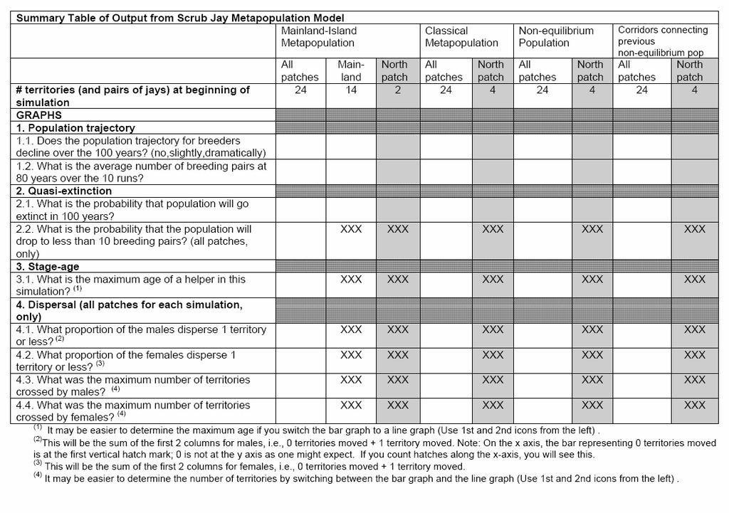
2 A BRIEF OVERVIEW OF THE PROGRAM This program (Jays ) is a spatially-explicit, individual-based population model designed to simulate the metapopulation dynamics of the Florida Scrub Jay. It was written by Bradley M. Stith, while he was a Ph.D. student in the Dept. of Wildlife Ecology and Conservation, University of Florida, Gainesville, Florida. A more complex version of this program has been used to assess the status of Scrub Jays state-wide. Demographic parameters in the model are based on data from a 30-year mark-recapture study of jays at Archbold Biological Station directed by G. Wolfenden and J. Fitzpatrick. Reproductive success in territories has been monitored since1969. The dispersal behavior of scrub jays in the model is based on dispersal events recorded from sightings of marked birds in this long-term study and on movement patterns documented by Brad Stith using radio-telemetry. As expressed on the program s manual, simulations take place on a landscape provided by a geographic information system (GIS) file. (For the state-wide analysis, Brad used GIS coverage of scrub for the entire state. For our class, he designed simple landscapes to illustrate outcomes for different metapopulation types.) In the model, male and female jays live within territories, each territory having its own set of demographic parameters. Individual jays progress through 4 stages (juvenile, 1-year helper, older helper, and breeder) for both sexes. Breeder experience and presence of helpers may affect reproductive success. Helpers monitor neighboring territories and may take over the territory when breeders disappear from the territory; the outcome of competition between helpers for breeder openings is determined by simple dominance rules. Helpers also may leave on long distance dispersals, during which mortality and movement varies depending on land cover type. During the simulation, graphs of dispersal distances, stage-age structure, population trajectory, and quasi-extinction probabilities are displayed, and text descriptions of various events occurring during the simulation can be viewed and saved to an output file (Jays ver. 1.0a User Manual, pg. 4, Overview). During this exercise you will examine and compare the metapopulation dynamics for each of the following landscapes: (1) mainland-island metapopulation, (2) classical metapopulation, (3) one equilibrium population, and (4) non-equilibrium population connected by corridors. Model Number of Populations of Subpopulations Patch Sizes Numbers of territories/patch Habitat quality of territories Distance between patches Population parameters (e.g. survivorship, productivity, etc.) Mainland Island Metapopulation Classical Metapopulation Non-equilibrium Populations Non-equilibrium Populations Connected by Corridors 6 sub-populations 6 sub-populations 6 populations 6 sub-populations 1 large patch 5 small patches All patches equal size 14 on the large patch 2 on the small patches 4 in each patch Close enough together for some dispersal, but not close enough to form one demographic unit. All Equal Close enough together for some dispersal, but not close enough to form one demographic unit Patches are too far apart for successful dispersal between them Equal for all different models Same distances as in the non-equilibrium simulation but through habitat restoration all of the patches are linked with corridors

3 TO RUN A SIMULATION 1. Open the program Jays by double clicking on the program on the Desktop or following other instructions given in lab. 2. Maximize both windows by clicking on the open window icon on the upper right corner of the window. 3. Click on File. 4. Select Open Prev. Sim. (= previous simulation). There are 2 ways to start a simulation: 1) the easiest one is to start from a previous simulation file that contains all of the information necessary to start a simulation run; 2) to create a new simulation file by providing a GIS file, territory locations, and parameter setting. In this lab, we will only use approach 1). 5. Choose the file for the landscape that you wish to use. In the first exercise, you will choose mainlandisland.jay. Choose that now. Subsequent exercises will have corresponding file names (classical.jay, nonequilibrium.jay, and corridor.jay). The *.jay files have the population parameters (survivorship, dispersal distance, etc). If the landscape does not appear when you open the *.jay file, another window will appear with the question Where is the GIS file?. In this window, you will choose the GIS file (the appropriate.bmp file) for this simulation ( mainlandisland.bmp ). Subsequent exercises will have corresponding file names (classical.bmp, nonequilibrium.bmp, and corridor.bmp). 6. Look at the screen. For each simulation, a diagram of the landscape will appear on the screen (GIS screen). In the diagram, scrub habitat is represented by yellow. The habitat matrix (which is not suitable for jays) is shown in green. Water is illustrated in blue. Each box is a jay territory. At the beginning of the simulation, each territory contains a pair of breeding birds and helpers. As the simulation runs, birds disperse from the territories and mortality also occurs. Empty boxes represent empty territories. Territories are recolonized by dispersers when they can reach the territory. 7. When you open the program, 4 graphs will be available from data from the last simulation that was run (by whomever used the program last). These graphs may appear on the screen automatically. If not, you can open them by clicking on Graph above the landscape diagram. The easiest way to view a simulation is, before you begin the simulation, open all 4 graphs (the ones currently available), and tile them from the Menu (Window/Tile Vertically) in a way that you can see the landscape and the four graphs simultaneously. You will be able to see jays dispersing on the landscape and the data on the graphs changing during the simulation if you have everything nicely arranged on your screen before you start. Graphs can be displayed in two formats (vertical bar, line graphs). Sometimes data are easier to see as a bar, and at other times the lines are easier to read. To switch between graph formats, click on the buttons at the top left of the graph window. 8. Now, let s get ready to run a simulation. For this, you first should set the number of years for the simulation and the number of replicates. Click on Parameters, on the Menu, and then click on General/Output, or directly click the yellow button Par on the Icon s Toolbar. On the Years/Reps tab, set the number of years to 100 and the number of replications to 10. If these numbers are already set to 100 and 10 respectively, leave them as they are. Generally, modelers run 100 or 1000 replications. However, this requires a lot of computer time. Thus, we will use After setting the number of years and replicates for the simulation, click OK. Then, Go! on the top toolbar and select a speed (you can directly select the speed from the Icon s Toolbar). Choose Medium for the speed that you wish to view the simulation so you can see the movement of the birds on the GIS screen. You may change to Slow or Fast at any time. After you familiarize yourself with the screen, you may want to change the speed to Fast during the middle of the simulation to speed up the process. When you Click on Go/Speed, you will see a window that says Warning Save your changes? or Keep your previous statistics?. Just click on No and proceed. If you have already run a simulation, sometimes, even if you say No, the program will continue adding replicates to the last simulation (although it is not supposed to do so). For example, if you ran one simulation with 10 replicates, the second simulation could terminate with 20 replicates (10 from the previous simulation, and 10 from the current simulation). In cases where you run the simulation for 2nd time or more and you select to not save the statistics, the program should begin with replicate number 1. For our purpose, it does not matter if the simulations are added together. So ignore this problem if it occurs. 10. Watch the GIS screen as the simulation progresses, and try to interpret what the jays are doing. Each territory (box) has 2 adult birds at the top of the box and a sign for helpers at the bottom. If you watch carefully you can see one or more of the birds disappear (some adults die and helpers die and disperse). When the box turns red, there is an annual nesting event. If all boxes become empty in a patch, local extinction of jays has occurred in the patch. Graphs will be updated as the birds fly between territories on the screen and as birds die and are born, so the graphs are changing as you run the simulation! At the end of each 100 years (1 replicate), all the territories are filled with birds again and the simulation starts over. 11. As the simulation is running, you will see an indication of the state (# of replications, # of years within each replication and # of pairs being considered) at the bottom right corner of the screen. When the simulation is complete, a small window will pop up with a message indicating this. Press OK to exit this small window

4 A. Now let s look at the results of the simulation while it is running POPULATION TRAJECTORY graph. All patches: Examine the trajectory for all patches combined (the trajectory for all patches should be the first thing that appears on your screen when you click on this graph). If you happen to have data from one of the individual patches displayed, e.g., patch North, click on the button with the green patches above the population trajectory graph. Select All patches. The solid lines on this graph show the average number of breeding adults (blue) and the average number of helpers (red) for your 10 simulation runs at over the 100-year timeframe of the simulation. Data from all patches are included (i.e., 24 territories). You will see these lines changing during the simulations as each simulation is run and averaged with the previous simulation results. The dashed lines show one simulation run at a time. After each of the 10 simulations, this line will be erased and initiated again. If you watch closely you will see this. The dashed lines that are on the graph at the end of the 10 simulations are the lines for the last simulation only (i.e., simulation number 10). Answer questions 1.1. and 1.2. on the SUMMARY TABLE for All patches. Mainland: Click on the button with the green patches above the population trajectory graph for all patches. Select the Mainland. Answer questions 1.1. and 1.2. on the SUMMARY TABLE for Mainland. North Patch: Click on the button with the green patches above the population trajectory graph for all patches. Select the North Island (or patch). Answer questions 1.1. and 1.2. on the SUMMARY TABLE for North Island. 2. QUASI-EXTINCTION graph. NOTE: Before looking at the graph, read the EXPLANATORY TEXT BOX included on the next page. All patches: Examine the quasi-extinction graph for all patches combined (this should be the first thing that appears on your screen when you click on this graph). Answer questions 2.1. and 2.2. on the SUMMARY TABLE for All patches. Mainland: Click on the button with the green patches above the quasi-extinction graph for all patches. Select the Mainland. Answer question 2.1. on the SUMMARY TABLE for Mainland. North Patch: Click on the button with the green patches above the quasi-extinction graph for all patches. Select the North Patch. Answer question 2.1. on the SUMMARY TABLE for North Patch. 3. STAGE-AGE graph. All patches: This graph shows the proportion of breeders and male and female helpers at each age (1-20 years). Answer question 3.1. on the SUMMARY TABLE for All patches. 4. DISPERSAL graph. All patches: This graph shows the proportion of males and females that disperse different distances (0-25 territories). Dispersal is the movement of an individual from the territory where it was born to the territory where it breeds. Birds that move through the matrix but do not make it to a new patch to breed are not included as dispersers. Distance is given in number of natal territories crossed. Currently the radius of a territory is set at 6 pixels. Each pixel represents 30 m for a total territory radius of 180 m. Number of territories crossed is really the number of 180-m segments between their original territory and where they settle to breed, NOT the number of actual territories the bird flew over. The distance of matrix the bird flew over and the distance across the patches it flew over are counted. Note: The size of the territories can be changed under parameters for territories, for example, to simulate territory size in habitats with different quality (e.g., territories might be larger in lower quality habitat). Answer questions on the SUMMARY TABLE for All patches.

5 - 5 - A Brief Explanation of the Quasi Extinction Curve The quasi-extinction curve is a graphical representation of the probability of a population falling below some threshold population size. (Note: In this computer model, threshold population size is given in number of pairs of jays, rather than number of individuals). It is a relatively simple graph and can give insight into the stability of a population at certain sizes. For example, let s say a certain landscape contains 25 breeding territories of birds that are occupied by 25 pairs. Due to mortality, dispersal, and other such factors, probability is high that at some point the population will drop below 25 pairs. These probabilities also would be affected by habitat quality in the real world or if habitat quality were changed in our model. For example A in the graph below (dashed lines marked A), the probability that the population will drop below 20 pairs will be higher in low quality habitat (1.0 or 100%) than in high quality habitat (0.8 or 80%). Note how probabilities change with the number of pairs. In example B (dashed lines marked B), there is an 80% (0.8) probability that the low quality habitat population will drop below 10 pairs versus an extremely low probability in high quality habitat (somewhere below 0.2). These quasiextinction curves suggest that under the current conditions, the high quality habitat metapopulation will not reach extinction, or 0 breeding pairs. LOW QUALITY HABITAT HIGH QUALITY HABITAT The probability of reaching 0 pairs (complete extinction) is the point at which the line crosses the y axis. For example, if the line crosses the y axis at 0.30 (as in the low quality habitat), there is a 30% probability that the population will reach 0 and go extinct (i.e., in 3 of the 10 simulation runs the population would go extinct before reaching the end of the simulation in 100 years). If the line does not cross the y axis as in the high quality habitat, then this suggests that the population will not reach extinction under the set of conditions present in the model. Note: Sometimes the line forming the graph comes very near the y axis but does not touch the axis (see graph A below). In this case, the line should touch the y axis. This is just a small problem with the drawing program. You should just extrapolate out. In the graph A below, there would be a 20% chance of the population reaching 0. In graph B, there would be no chance of reaching extinction under the conditions in the model.

6 - 6 - DO NOT CLOSE the first simulation (mainland-island) because we will compare the graphs with the rest of the models. Just minimize the output screens. SECOND SIMULATION: Classical metapopulation You now will run a second simulation for a classical metapopulation. Start the second simulation by opening the program Jays as you did in the first simulation. If you try to start a second simulation by clicking on File open within the simulation screens from the simulation you have just run, you will get an error message. Run the classical metapopulation simulation using the instructions on pg.3 (i.e., follow the same procedure as for the previous simulation), but choosing the classical.jay file this time. If you are careful, you can then put all 8 graphs from the two simulations on the screen at once so that you can compare between simulations. After you finish the simulation, answer the same questions as in the previous one, but just for all patches combined and for the North patch (i.e., not for the Mainland patch, see Table at the end). DO NOT CLOSE the first 2 simulations (mainland-island and classical) because we will compare these graphs with the rest of the models. Just minimize the output screens. THIRD SIMULATION: Non-equilibrium population. You now will run a third simulation for a non-equilibrium population. Start the third simulation by opening the program Jays as you did in the first simulation. If you try to start a second simulation by clicking on File open within the simulation screens from the simulation you have just run, you will get an error message. Run the non-equilibrium simulation using the instructions on pg.3 (i.e., follow the same procedure as for the first and second simulation), but choosing the nonequilibrium.jay file this time. After running all three simulations you can pull up any sets of graphs that you want to compare (for example, population trajectories for all three simulations, all graphs for 2 of the simulations, etc.). After you finish the simulation, answer the same questions as in the previous one (i.e., for all patches and the North patch, see Table at the end). DO NOT CLOSE the 3 previous simulations (mainland-island, classical and non-equilibrium) because we will compare these graphs with the rest of the models. Just minimize the output screens. FORTH SIMULATION: Non-equilibrium populations connected by corridors. You are now going to run the fourth simulation. Minimize the previous simulation so that you can look at it later and start the forth simulation by opening the program Jays as you did in the first simulation. If you try to start a second simulation by clicking on File open within the simulation screens from the simulation you have just run, you will get an error message. Run the non-equilibrium populations connected by corridors simulation using the instructions on pg.3 (i.e., follow the same procedure as for the previous simulation), but choosing the corridor.jay file this time. After running all four simulations you can pull up any sets of graphs that you want to compare (for example, population trajectories for all four simulations, all graphs for 2 of the simulations, etc.). After you finish the simulation, answer the same questions as in the previous one (i.e., for all patches and the North patch, see Table at the end).

7 Lab Exercise (50 points) NAME: (include your name on all the pages) B. Using the table you have filled in, compare the results for the different types of metapopulations for each question. Include this Summary Table with the answers to these questions when you turn in your Lab Exercise. 1) Which landscapes are most similar in terms of population trajectories and average number of breeding pairs at 80 years for the total population (all patches combined)? Which are the most different? (Note: If you have two sets that are very similar, list both.) SIMILAR DIFFERENT 2) Which metapopulation type has the highest probability that the population will drop to less than 10 breeding pairs for all patches? Which has the lowest probability? Why? HIGHEST LOWEST 3) Compare the value of probability of extinction for the Mainland to the value for the North patch. How does patch size influence probability of extinction of subpopulations? 4) Compare the population trajectory in the North patch for the year of the last run for breeders (blue dashed line) for Classical vs. Non-equilibrium. a) How many times did the breeders in the North patch go extinct and recolonize the patch within the 100-yr run for each metapopulation type? (Hint: Look at how many times the dashed blue line hit the x- axis. If the blue line hits the x axis and never appears again, the subpopulation is extinct and there is no recolonization. If the blue line hits the x axis and then starts up again a little later, recolonization has occurred.). b) What is the role of demographic rescue in each of these types of metapopulations? (Hint: Think about how extinction/recolonization is different from demographic rescue). 5) Landscape structure can facilitate or inhibit dispersal. Which landscape facilitates long-distance dispersal (more than 8 territories) the strongest? Why? How does dispersal influence population persistence? (Hint: compare the probability that the population will drop to less than 10 breeding pairs between non-equilibrium and corridor models) Note: The probability of jays dispersing did not change between simulations but the probability that this dispersal would be successful did change because of the habitat configuration (i.e., the probability that they would encounter an open territory before they died differed between simulations). 6) Close the previous non-equilibrium simulation. (Note: you must close this simulation to run it again). Start a new simulation by opening the program Jays again as you did above. Run a new nonequilibrium simulation using the instructions on pg.3 (i.e., follow the same procedure as for the previous simulations), but choosing the nonequilibrium.jay file and setting the number of years to 50 this time (Step 8 on pg.3). After running this simulation, look at the results for the 1st non-equilibrium simulation (100 years) on the Summary Table. How did the probability of the population of going extinct change when we decreased the number of years for the simulation (all patches)? What consequences for the species conservation could you infer from considering 50 vs. 100 years as a time frame? 7) There are many small isolated patches of scrub habitat in Florida, and scrub jays would not persist unless management actions are taken. Based on your simulations, what management would you suggest (if any) for these populations? 8) Can you suggest 2 reasons why one should be cautious in interpreting the output of the models for management?

8 - 8 -