The Pennsylvania State University. The Graduate School. College of Engineering A NEW METRIC TO PREDICT LISTENER ENVELOPMENT BASED ON

Transcription

1 The Pennsylvania State University The Graduate School College of Engineering A NEW METRIC TO PREDICT LISTENER ENVELOPMENT BASED ON SPHERICAL MICROPHONE ARRAY MEASUREMENTS AND HIGHER ORDER AMBISONIC REPRODUCTIONS A Dissertation in Acoustics by David A. Dick 2017 David A. Dick Submitted in Partial Fulfillment of the Requirements for the Degree of Doctor of Philosophy December 2017

2 ii The dissertation of David A. Dick was reviewed and approved* by the following: Michelle C. Vigeant Assistant Professor of Acoustics and Architectural Engineering Dissertation Advisor Chair of Committee John F. Doherty Professor of Electrical Engineering Daniel A. Russell Professor of Acoustics Director of Distance Education for the Graduate Program in Acoustics Victor W. Sparrow Professor of Acoustics Director of the Graduate Program in Acoustics Bill Rabinowitz Manager of Acoustics Research, Bose Corporation Special Member *Signatures are on file in the Graduate School

3 iii ABSTRACT The objective of this work was to create a new metric to predict listener envelopment (LEV), the sense of being surrounded by the sound field, based on 32-channel spherical microphone array measurements taken in a number of venues and a series of listening tests. A spherical microphone array was used to investigate LEV because it can be used for a) high resolution spatial analysis of the sound field in full 3D via beamforming techniques, and b) subjective listening tests using 3D reproductions of the sound fields over a loudspeaker array via Ambisonics. This work is comprised of three separate studies: a first study validating the spherical microphone array measurement system, a second study investigating LEV in a 2,000- seat concert hall, and a third study in which a new metric is proposed to predict LEV based on listening tests using measurements obtained in seven additional halls. A study was conducted to validate the spherical microphone array measurement system. Spatial room impulse response (IR) measurements were taken in a 2500-seat auditorium to determine how room acoustic metrics measured with a spherical microphone array compare to those measured with the traditional microphone setup (an omnidirectional and figure-8 microphone pair). Measurements were obtained at six receiver locations with three repetitions each to evaluate repeatability. The metrics considered in this study were: reverberation time (T30), early decay time (EDT), clarity index (C80), strength (G), lateral energy fraction (J LF) and late lateral energy level (L J). For the spherical array measurements, the omnidirectional (monopole) and figure-8 (dipole) patterns were extracted via spherical harmonic beamforming. The measurements were found to be consistent both across repetition and microphone configuration. The results from this study indicate that spherical microphone arrays can be used to both measure existing LEV metrics, and to develop a new metric to predict LEV. An LEV study was conducted using spherical microphone array IRs obtained in a 2,000-seat concert hall in several receiver locations and hall absorption settings. The IRs were analyzed using a 3 rd order plane wave decomposition (PWD) beamformer. Additionally, the IRs were convolved with anechoic music and processed for 3 rd order Ambisonic reproductions and

4 iv presented to subjects over a 30-loudspeaker array. Instances were found in which the energy in the late sound field did not correlate with LEV ratings as well as energy in a 70 to 100 ms time window. Follow-up listening tests were conducted with hybrid IRs containing portions of a highly enveloping IR and a highly unenveloping IR with crossover times ranging from ms. Additional hybrid IRs were studied wherein portions of the spatial IRs were collapsed into all frontal energy with crossover times ranging from ms. The tests confirmed that much of the important LEV information exists in the early portion of these IRs. In a final LEV study, spherical microphone array IRs were obtained in seven additional halls of various sizes and shapes. The IRs were used for listening tests that included stimuli that were presented as-measured, which included level differences, stimuli that were equalized for level differences, and hybrid stimuli generated by combining portions of enveloping IRs and unenveloping IRs. A new metric was developed named mid-late spatial energy, J S, by integrating energy from a 3 rd order PWD of the room IRs as a function of frequency, azimuthal angle, elevation angle, and time, and adjusting the integration limits to maximize correlation between integrated energy and LEV ratings. The difference in overall level between halls was found to be highly correlated with the perception of LEV, but for level-equalized stimuli the correlation was maximized by integrating energy from 60 ms to 400 ms, rejecting sound from the front ±20 in azimuth and rejecting sound from ±70 in azimuth behind the listener. This new metric has a higher correlation with LEV ratings than the currently used metric of late lateral energy level, L J.

5 v TABLE OF CONTENTS List of Figures...xi List of Tables... xix Acknowledgements... xx Introduction Listener Envelopment (LEV) Early History of LEV Impact on LEV from energy other than late lateral arrivals Other Proposed LEV Metrics LEV Summary Spherical Microphone Arrays Wave equation in spherical coordinates Spherical Fourier Transform of Microphone Array Signals Scattering off of a rigid sphere Beamforming Ambisonics Spherical Harmonics Format Ambisonic Decoding Max-RE Decoding Nearfield Compensation AURAS Facility Layout AURAS Ambisonic Decoder Ambisonic Performance Dissertation Outline A Comparison of Measured Room Acoustics Metrics Using a Spherical Microphone Array and Conventional Methods... 27

6 vi 2.1 Introduction Room Acoustics Metrics Measurement Uncertainty Spherical Microphone Array Processing and beamforming Measurements Measurement Hardware Anechoic Chamber Directivity and Frequency Response Measurements Impulse Response Measurements in Eisenhower Auditorium Data Processing Microphone frequency response compensation Rotating the dipole Room acoustic metric calculation Results Measurement Repeatability of the Two Microphone Configurations Differences in Measured Room Acoustics Metrics between Microphone Configurations Conclusions Acknowledgements An Investigation of Listener Envelopment Utilizing a Spherical Microphone Array and Third-Order Ambisonics Reproduction Introduction Spherical Array Beamforming Ambisonics Reproduction Room Impulse Response Measurements Measurement Hardware Room IR Measurements Stimulus Reproduction Auralization and Reproduction of Acoustic Sound-fields (AURAS) Loudspeaker Array... 67

7 vii Validation Listener Envelopment Subjective Listening Test 1: Comparison of hall seats and absorption settings Subjective Listening Test 1 Results Beamforming Analysis of the measured Impulse Responses Listener Envelopment Subjective Listening Test 2: Listening Test Using Hybrid IMPULSE Responses Hybrid IR subjective test design Results for hybrid IRs containing portions of an unenveloping IR and an enveloping IR Results for hybrid IRs with removed spatial components Conclusions Acknolwedgement Appendix A: Calculating Metrics from spherical microphone array IR Measurements Front Back Ratio (FBR) Spatially Balanced Center Time (SBTs) A New Metric to Predict Listener Envelopment based on Spatial Impulse Response Measurements and Subjective Listening Tests Introduction Spherical Microphone Array Beamforming Ambisonics Reproduction Spatial Room IR Measurements Measurement Hardware Spherical microphone array Three-way omnidirectional sound source Details of the Seven Measured Halls and the Receiver Locations Subjective Study using Ambisonic Reproductions of spatial IRs Subjective listening test stimuli Test set 1: IRs from Seven different halls as measured

8 viii Test set 2: IRs from Seven different halls equalized for level Test set 3: High-LEV (HLEV) and Low-LEV (LLEV) hybrid IRs Test set 4: LLEV&HLEV hybrid IRs Subjective Study Results Statistical Analysis of LEV Ratings Results: Set 1 IRs from 7 different halls as measured Results: Set 2 IRs from 7 different halls equalized for level Results: Set 3 H-LEV&L-LEV Hybrid IRs Results: Set 4 L-LEV&H-LEV Hybrid IRs Metric Development Azimuthal Angular Dependence LEV Rating Correlation Excluding Frontal energy LEV Rating Correlation Excluding Rear energy Elevation Angular Dependence Time Dependence LEV Rating Correlation Varying Early Time Cutoff LEV Rating Correlation Varying Late Time Cutoff Overall Metric Performance relative to late lateral energy level and strength Performance with order reduction Effect of the Early Sound Field Conclusions Conclusions Results Summary Future Work Appendix A: Calculation of Mid-Late Spatial Energy (JS) Appendix B: Three Way Omnidirecitonal Sound Source

9 ix B.1 Introduction B.2 Directivity of the source components B.2.1 Subwoofer Directivity B.2.2 Mid-frequency dodecahedron directivity B.2.3 High-frequency dodecahedron directivity B.3 Omnidirectional source validation with room measurements B.3.1 Measurement uncertainty due to source rotation B Energy as a function of source rotation B Room acoustic metrics as a function of source rotation B.3.2 Stacked vs. coincident configurations B Energy differences between stacked and coincident configurations B Room acoustic metrics for the stacked and coincident orientations B.4 Summary Appendix C: Complete Set of Directivity Plots of the Mid-Frequency and High-Frequency Dodecahedrons 151 C.1 High-Frequency Dodecahedron: 3D Octave Band Plots (1,000 16,000 Hz) C.2 High-Frequency Dodecahedron 3D Third-Octave Band Plots (1,000 16,000 Hz) C.3 High-Frequency Dodecahedron: 2D Polar Plots (Azimuthal Plane) Third-Octave Bands (1,000 20,000 Hz) C.4 High-Frequency Dodecahedron: 2D Polar Plots (0 Elevation Plane) Third-Octave Bands (1,000 20,000 Hz) C.5 High-Frequency Dodecahedron: 2D Polar Plots (90 Elevation Plane) Third-Octave Bands (1,000 20,000 Hz) C.6 Mid-Frequency Dodecahedron: 2D Polar Plots (Azimuthal Plane) Third-Octave Bands (125 20,000 Hz) C.7 Mid-Frequency Dodecahedron: 2D Polar Plots (Elevation Plane) Third-Octave Bands (125 20,000 Hz)

10 x Appendix D: Subjective Test Tutorial Example References

11 xi LIST OF FIGURES Figure 1-1: Angular distribution of loudspeakers used to develop LJ (Fig. 1, Bradley and Soulodre, 1995 [10]) Figure 1-2: Plots of the real-valued spherical harmonics for orders n = 0, 1, 2, and Figure 1-3: Plane wave modal coefficients for a sphere of radius a = 4.2 cm Figure 1-4: Beam pattern of a truncated plane wave of order N = Figure 1-5: Block diagram for the overall beamforming system (adapted from Fig. 5.3, Fundamentals of Spherical Array Processing, Rafaely, 2015 [26]) Figure 1-6: Energy received at the listening location from a plane wave produced using 3 rd order Ambisonics for basic decoding (left) and Max-r E decoding (right) Figure 1-7: The AURAS loudspeaker array (a), and the distribution of the 30 loudspeakers in the array (b) Figure 1-8: Magnitude, direction, and angular error of the r v vector, plotted in the Ambisonics Decoder Toolbox Figure 1-9: Magnitude, direction, and angular error of the re vector, plotted in the Ambisonics Decoder Toolbox Figure 2-1: Microphones used in this study. (a) Eigenmike em32 spherical microphone array and (b) a Brüel & Kjær (B&K) Type 4192 omnidirectional and Sennheiser MKH30 figure-8 microphone pair Figure 2-2: Custom microphone stand used for accurate and precise placement of microphones. The photo on the left shows the stand being used to place the microphone and the one on the right shows the microphone in the final position Figure 2-3: Microphone directivity plots for the Sennheiser MKH30 figure-8 microphone (left) and Eigenmike em32 beamformed dipole pattern (right) Figure 2-4: Deviations from ideal polar patterns: Sennheiser MKH30 figure-8 microphone directivity versus a perfect dipole (a), Eigenmike em 32 beamformed dipole versus a perfect dipole (b) and Eigenmike em32 beamformed omnidirectional pattern versus a perfect omnidirectional (c) pattern Figure 2-5: Receiver positions in 2500-seat Eisenhower Auditorium

12 xii Figure 2-6: Eigenmike (blue) and Sennheiser MKH30 (red) equalization filter magnitude response. Target responses are shown as dashed lines, and realized filters fit to the target responses are shown as solid lines. The Eigenmike target and actual filter are nearly identical, which is why the dashed line is difficult to see in the figure Figure 2-7: Standard deviation of the three repeated measurements for each metric at each receiver location for the omnidirectional and figure-8 microphone pair (solid lines) and the Eigenmike array (thin-dashed lines) configurations. The thick-dashed red lines on each plot represent the respective 1 JND for each metric. All standard deviations were found to be well below 1 JND for each metric and all receiver positions, with the exception of a few cases for EDT Figure 2-8: Differences between the omnidirectional and figure-8 microphone pair and the Eigenmike array configurations for all six metrics measured at all six receiver locations. The thick-dashed red lines on each plot represent the respective 1 JND for each metric. All differences were found to be within 1 JND, with the exceptions of a single point in C80, and several points in EDT at high frequencies Figure 2-9: The energy decay curves and associated early decay time slope fits for R3 in the 2 khz octave band shown for the omnidirectional B&K microphone (blue) and Eigenmike array (red). Note the spikes in the curve as denoted with the orange ovals, which are likely due to differences in where the centers of each microphone were positioned Figure 2-10: Early decay time calculated for Eigenmike individual microphone capsules (green), and early decay time calculated for the omnidirectional B&K microphone (blue) at R Figure 3-1: Spherical harmonic functions of order n and degree m, up to n = 3. For convenience, the real-valued spherical harmonics are shown, where red indicates a positive value and blue indicates a negative value Figure 3-2: Measurement hardware used for the IR measurements: (a) Eigenmike spherical microphone array (mh acoustics em32), (b) B&K binaural mannequin (type 4100-D), and (c) B&K dodecahedron loudspeaker (type 4292) Figure 3-3: Receiver locations in the Peter Kiewit Concert Hall Figure 3-4: The AURAS loudspeaker array (a), and the distribution of the 30 loudspeakers in the array (b) Figure 3-5: Block diagram for Ambisonic reproduction... 68

13 xiii Figure 3-6: Radial filters convolved with microphone equalization that are applied after encoding the spherical array s individual microphone signals to Ambisonic signals Figure 3-7: Comparison of 3 rd order simulated plane wave with max-r E decoding, representative of a plane wave produced in the AURAS facility above 1.3 khz (left) to a plane wave produced in the AURAS facility measured at 2 khz (right). Pressure magnitude is shown on a linear scale normalized to a maximum value of Figure 3-8: Mean LEV ratings for the four test sets. Error bars depict standard errors Figure 3-9: Comparison of the late sound field at 1 khz (80 ms to ) between receiver positions with similar LEV ratings (R3 and R8 from Set 2), with 0 azimuth pointing toward the stage and 0 elevation pointing straight up. Sound pressure level is shown ranging from -10 db to 0 db, where 0 db is the maximum level of both sound fields (overall level differences are maintained between the top and bottom plots). The images on the left show the energy distributions over spheres, while the images on the right show the same information, but flattened onto a 2-D plot (similar to an unraveled a map.) Energy at R3 is concentrated toward the front (R3 is underneath a balcony), whereas energy at R8 is more evenly distributed throughout the sphere (R8 is in the top balcony) Figure 3-10: Comparison of the late sound field at 1 khz between receiver positions with different LEV ratings (R9 and R10 from Set 1), with 0 azimuth pointing toward the stage and 0 elevation pointing straight up. Sound pressure level is shown ranging from -10 db to 0 db, where 0 db is the maximum level of both sound fields (overall level differences are maintained between the top and bottom plots). The spatial distribution of late energy is similar between the two receivers yet the LEV ratings of these stimuli were significantly different Figure 3-11: Comparison of the sound field from 70 to 100 ms at 1 khz between receiver positions with similar LEV ratings (R3 and R8 from Set 2), with 0 azimuth pointing toward the stage and 0 elevation pointing straight up. Sound pressure level is shown ranging from -10 db to 0 db, where 0 db is the maximum level of both sound fields (overall level differences are maintained between the top and bottom plots). The energy at both receiver positions have a similar level and distribution in terms of lateral, behind, and overhead sound. The frontal energy does differ by 3 db between the pair, but it is assumed that energy arriving from the front does not influence LEV Figure 3-12: Comparison of the sound field from 70 to 100 ms at 1 khz between receiver positions with different LEV ratings (R9 and R10 from Set 1), with 0 azimuth pointing toward the stage and 0 elevation pointing straight up. Sound pressure level is shown ranging from -10 db to 0 db, where 0 db is the maximum level of

14 xiv both sound fields (overall level differences are maintained between the top and bottom plots). R9 has a much stronger energy level from behind, which may be contributing to the perceived LEV Figure 3-13: Half Hann 2.5 millisecond time windows used to mix two IRs (left), and example resulting hybrid IR (right). The early window and corresponding IR are shown in solid blue, and the late window and corresponding IR are shown in dotted and solid green, respectively Figure 3-14: Modified IRs using the early part of R10 (highly unenveloping) and the late part of R3 (highly enveloping) with crossover times ranging from 40 ms (highly enveloping) to 140 ms (highly unenveloping) Figure 3-15: Modified IRs using the early part of R3 (highly enveloping) and the late part of R10 (higly unenveloping) with crossover times ranging from 40 ms (highly enveloping) to 140 ms (highly unenveloping) Figure 3-16: Results of the modified IR test in which the early part of the IR is presented in full 3D, and the late part of the IR is reproduced from a single loudspeaker Figure 3-17: Results of the modified IR test in which the late part of the IR is presented in full 3D, and the early part of the IR is reproduced from a single loudspeaker Figure 4-1: The AURAS loudspeaker array (a), and the distribution of the 30 loudspeakers in the array (b) Figure 4-2: Three-way omnidirectional sound source components: subwoofer (left), midfrequency dodecahedron (middle), and high-frequency dodecahedron (right). Note that the photos are not to scale relative to each other. The subwoofer has 25-cm drivers, the mid-frequency source has 10-cm drivers, and the high-frequency source has 1.9-cm drivers Figure 4-3: Top-down view diagram of receiver positions measured in each hall. R4, shown as the blue diamond, is the receiver position used for the subjective tests in this study Figure 4-4: High-LEV (HLEV) and Low-LEV (LLEV) hybrid IR with a crossover time of 200 ms Figure 4-5: LEV ratings for Set 1: IRs from 7 different halls as measured. Colored-shapes were added to indicate statistically significant pairs at p < 0.05, where stimuli that share the same colored-shape are not significantly different (note that some data points have multiple colored-shapes)

15 xv Figure 4-6: Set 1 LEV ratings vs. late lateral energy level. LEV ratings were found to have a high correlation with L J, although this correlation is primarily due to level differences between the stimuli Figure 4-7: LEV ratings for Set 2: IRs from 7 different halls, which are the same halls as used in Set 1, but equalized for level. Colored-shapes were added to indicate statistically significant pairs at p < 0.05, where stimuli that share the same coloredshape are not significantly different (note that some data points have multiple colored-shapes) Figure 4-8: Set 2 LEV rating vs. L J. The correlation between L J and LEV rating for Set 2 (R 2 = 0.77, p < 0.004) is lower than in Set 1 (R 2 = 0.94, p < 0.001) after normalizing the overall A-weighted level Figure 4-9: LEV ratings for Set 3. Colored-shapes were added to indicate statistically significant pairs at p < 0.05, where stimuli that share the same colored-shape are not significantly different. LEV ratings for crossover times 80 ms and lower are not significantly different than the LEV rating for the whole L-LEV IR Figure 4-10: Set 3 LEV rating vs. L J. Each data point is labeled for its crossover time. The correlation between LEV and L J is high (R 2 = 0.95), primarily because all data points up to the 80 ms crossover time share the same L J value and have similar LEV ratings Figure 4-11: LEV ratings for Set 4. Colored-shapes were added to indicate statistically significant pairs at p < 0.05, where stimuli that share the same colored-shape are not significantly different Figure 4-12: Set 4 LEV rating vs. L J. Each data point is labeled for its crossover time. Correlation is much lower than in previous sets (R 2 = 0.73) because the four data points up to the 80 ms crossover point have identical values of L J, but very different LEV ratings Figure 4-13: Energy grid for Hall 5, the 1200-seat shoebox hall, in the 1 khz octave band summed from 60 ms to 200 ms. Energy is shown in db relative to the maximum. with 0 azimuth pointing toward the stage and 0 elevation pointing straight up. The images on the left show the energy distributions over spheres, while the image on the right show the same information, but flattened onto a 2-D plot (similar to an unraveled map.) Figure 4-14: Energy grid for Shoe1200 in the 1 khz octave band summed from 200 ms to 500 ms. Energy is shown in db relative to the maximum. The azimuthal variation is much lower than the variation from 60 ms to 200 ms as shown in Figure

16 xvi Figure 4-15: Correlation coefficient vs. rejection angle for Set 2 in the 1 khz octave band for both front sound rejection (blue line) and rear sound rejection (orange line). The maximum R 2 values are circled for each case. The correlation for rejecting the front sound is maximized at 20. The correlation for rejecting the rear sound is maximized at 70 degrees, which is a larger rejection angle than was found for the front energy. Additionally, rejecting the rear sound has a higher correlation coefficient than rejecting the front sound Figure 4-16: Correlation coefficient vs. early time cutoff for Set 2 in the 1 and 2 khz octave bands. The correlation is maximized when a portion of the early sound field is included in the integration. The maximum R 2 values are circled for each of the octave bands shown Figure 4-17: Correlation coefficient vs. late time cutoff. Correlation increases slightly as the late time cutoff is increased, and asymptotically reaches a maximum around 400 ms Figure B-1: Low frequency measurement of a Brüel & Kjær OmniPower Type 4292 loudspeaker in an anechoic chamber Figure B-2: Directional response of Brüel & Kjær OmniPower Type 4292 loudspeaker [OmniPower datasheet, bksv.com] Figure B-3: Allowable deviations from omnidirectional directivity per octave band [ISO :2009, adapted from Table 1] Figure B-4: Three-way omnidirectional sound source components: subwoofer (left), midfrequency dodecahedron (middle), and high-frequency dodecahedron (right). Note that the photos are not to scale relative to each other Figure B-5: Three-way crossover filters for the omnidirectional sound source Figure B-6: Free-field measurements of the subwoofer. Measurements on-axis with the drivers are in red and blue, and measurements with the source rotated 90 off-axis are shown in green and cyan Figure B-7: Directivity of the mid-frequency dodecahedron source rotated in azimuth Figure B-8: Directivity of the mid-frequency dodecahedron source rotated in elevation Figure B-9: 3D directivity plots of the high-frequency dodecahedron source in db Figure B-10: Receiver locations in Eisenhower Auditorium for the omnidirectional source validation measurements

17 xvii Figure B-11: Early energy differences as a function of source rotation in db Figure B-12: Late energy differences as a function of source orientation in db Figure B-13: Differences in early decay time (EDT) as a function of source orientation. JNDs for each octave band are denoted by the orange lines, where the JND for EDT is 5% Figure B-14: Differences in reverberation time (T30) as a function of source orientation. JNDs for each octave band are denoted by the orange lines, where the JND for T30 is 5% Figure B-15: Differences in clarity index (C80) as a function of source orientation. JNDs for each octave band are denoted by the orange lines, where the JND for C80 is 1 db Figure B-16: Differences in early lateral energy fraction (J LF) as a function of source orientation. JNDs for each octave band are denoted by the orange lines, where the JND for J LF is Figure B-17: Differences in late lateral energy level (L J) as a function of source orientation. JNDs for each octave band are denoted by the orange lines (the JND of L J is assumed to be 1 db, the JND for strength, since the JND for L J is not known) Figure B-18: Three-way omnidirectional source in the stacked configuration Figure B-19: Three-way omnidirectional source in the coincident configuration, three separate measurements Figure B-20: Difference in early energy between the stacked configuration and coincident configuration Figure B-21: Difference in late energy between the stacked configuration and coincident configuration Figure B-22: Differences in early decay time (EDT) for the stacked vs. coincident configurations. JNDs for each octave band are denoted by the orange lines, where the JND for EDT is 5% Figure B-23: Differences in reverberation time (T30) for the stacked vs. coincident configurations. JNDs for each octave band are denoted by the orange lines, where the JND for T30 is 5%

18 xviii Figure B-24: Differences in clarity index (C80) for the stacked vs. coincident configurations. JNDs for each octave band are denoted by the orange lines, where the JND for C80 is 1 db Figure B-25: Differences in late lateral energy level (L J) for the stacked vs. coincident configurations. JNDs for each octave band are denoted by the orange lines (the JND of L J is assumed to be 1 db, the JND for strength, since the JND for L J is not known)

19 xix LIST OF TABLES Table 3-1: Correlation coefficients for different metrics as LEV predictors for Set Table 4-1: Details about the seven halls measured as a part of this study Table 4-2: Approximate dimensions the seven halls measured as a part of this study Table 4-3: Correlation coefficients between the new metric and mean LEV of the four test sets. All correlation coefficients shown are significant at p < 0.05 and the nonsignificant regressions are denoted by NS Table 4-4: Correlation coefficients between LEV rating and L J and the correlation coefficients between LEV rating and the new metric. All correlation coefficients shown are significant at p < 0.05 and the non-significant regressions are denoted by NS

20 xx Acknowledgements I would like to thank my thesis committee members: Drs. Sparrow, Russell, Doherty, and Rabinowitz for all of their comments, suggestions, feedback, and discussions over the last several years. I would also like to thank Chris Ickler for his helpful discussions on listener envelopment. Thanks to the professors and staff in the Graduate Program in Acoustics for providing an excellent acoustics education. Thanks to the students who have contributed to this project, including Matthew Neal, Carol Tadros, and Colton Snell. Huge shout out to Matthew Neal, who has been working on this project since the beginning and was instrumental in the construction of the loudspeaker array, conducting measurements, creating GUIs, and more. I m excited to see his progress as he continues this work for is Ph.D. My research involved a plethora of measurements in different halls, and I couldn t have made them without the help from my friends. Thank you, Matthew Neal, Martin Lawless, Rachael Romond, Will Doebler, Peter Moriarty, Matthew Blevins, Laura Brill, Hyun Hong, Joonhee Lee, and Zhao Ellen Peng. The measurements would also not be possible without access to the halls, provided by Tom Hesketh, Ed Hurd, Chris Ball, Johanna Kodlick, Vonny Boarts, John Coffelt, and Jack and Carolyn Zybura. I want to express my gratitude to my friends and family both in State College and elsewhere, especially my parents and my wife Barbara. I dragged Barbara all the way to State College from Massachusetts for a few years, and I could not have done this without her love, support, and encouragement. To all SPRALites and Research Westians, it s been great getting to know you all both inside and outside of work. Finally, I would like to express my greatest thanks to my advisor and chair of my committee, Dr. Michelle Vigeant. I first worked with her as an undergraduate student at the University of Hartford nearly 10 years ago. She encouraged me to pursue graduate studies, which influenced my decision to take distance education coursework in the Graduate Program in Acoustics while I was working full time. When she came to Penn State, she contacted me about this project and asked if I had ever thought about pursuing a Ph.D., which was something I didn t think I was

21 xxi capable of at the time. I took a chance when I left my job to come to Penn State, but it worked out well and I learned a ton about acoustics and conducting research. I would like to thank Michelle for believing in me, for her mentorship, for her dedication in meeting with students, and for her pursuit of perfection in conference presentations and publications. The work presented in this dissertation was sponsored by the National Science Foundation (NSF) award # Approval for human subjects testing was obtained from Penn State s Institutional Review Board (IRB #41733).

22 1 Introduction An important aspect of the overall impression of a concert hall is the spatial impression of the hall, which includes listener envelopment (LEV), the sense of being fully immersed in the sound field [1] [2]. Other important attributes include reverberance, bassiness, proximity, definition, and clarity [2]. The spatial impression of concert halls and LEV have been studied for decades, and objective measures have been proposed to predict the perception of LEV. The purpose of this work was to investigate LEV using state-of-the-art measurement techniques utilizing a compact spherical microphone array and subjective studies using 3D reproduction of the sound fields via higher order Ambisonics. The results from the objective analysis of the sound fields and subjective listening tests were used to inform the development of a new metric to predict LEV based on a spherical harmonic decomposition of the sound field. Utilizing measurements obtained with a spherical microphone array has several advantages over conventional microphones that are commonly used. The impulse response (IR) measurements made using a spherical array can be used for an objective analysis of the sound field in full 3D via beamforming techniques in the spherical harmonics domain. The spherical harmonic beamforming yields a much higher spatial resolution than conventional measurement methods, which primarily use microphones with a first-order dipole or cardioid type pattern. The IRs can also be processed using Ambisonics for subjective listening tests with 3D reproductions of the sound fields over a loudspeaker array. Previously, LEV was studied primarily using simulated sound fields reproduced over a limited number of loudspeakers, which are less representative of the actual sound field experienced in a concert hall. 1.1 LISTENER ENVELOPMENT (LEV) Early History of LEV Research aimed at understanding the spatial perception in performing arts spaces initially focused on the directional dependence of early reflections. Originally, the sense of spaciousness was thought to be primarily associated with reverberation, but in the late 1960 s, it was found

23 2 that the spatial impression was heavily influenced by early reflections [3, 4, 5]. It was proposed that the spaciousness depended on the arrival direction of early reflections, and that stronger early lateral reflections were related to a quality referred to as spatial responsiveness [6]. Further work led to the development of the objective metric Early Lateral Energy Fraction, J LF (original notation was LF) [7], J LF = 80ms p 2 (t)dt 5 ms L 80ms, (1-1) p 2 (t)dt 0ms the ratio between the early lateral energy and the total early energy in the first 80 ms, which was found to be correlated with the subjective level of spatial impression [7]. A second metric that has been shown to correlate with spatial impression is the interaural cross correlation coefficient (IACC early), which is obtained from the cross-correlation of the left and right ears of a binaural IR [8]: IACC = t2 p left(t)p right (t + τ)dτ t1 t2 2 2 p left (t)dt p right (t)dt t1 max for 1 ms < τ < 1 ms (1-2) where t 1 is 0 and t 2 is 80 ms for IACC early. Later work in spaciousness proposed that the spatial impression of a hall contains two distinct perceptions: apparent source width (ASW), which is the sense of how wide or narrow the sound image appears to a listener, and LEV, the sense of being immersed in and surrounded by the sound field [9]. ASW has since been shown to be related to early lateral reflections, which can be predicted using IACC and J LF, while LEV has been shown to be related to late lateral energy [10]. Seminal work on LEV was conducted by Bradley and Soulodre in the early 1990 s [10, 11]. Using five loudspeakers distributed in the front half of the horizontal plane, shown in Figure 1-1, sound fields were generated with a small number of early reflections that were kept constant, and varied certain aspects of the late sound field: the reverberation time (T30), the early-to-late sound energy ratio (C80), and the strength of the late sound field (G Late). The angular distribution of the late sound was also varied, which was accomplished by playing the late sound either out

24 3 of a single frontal loudspeaker, three frontal loudspeakers spanning 70, or five frontal loudspeakers spanning 180. A subjective study showed that the parameters with the highest correlation to LEV were angular distribution and overall late level. These results were used to develop a metric to predict LEV called late lateral energy level, L J (prior notations GLL, LG, and LG 80 ) [10]: L J = 10 log 10 [ p 2 (t)dt 80ms L ] [db], (1-3) p 2 10 (t)dt 0 where p L(t) is the room IR measured with a figure-of-eight microphone, and p 10(t) is the IR of the sound source normalized at a distance of 10 meters away in a free field. Figure 1-1: Angular distribution of loudspeakers used to develop L J (Fig. 1, Bradley and Soulodre, 1995 [10]). While a strong correlation was found between this metric and LEV, it should be noted that this study used a small number of loudspeakers spanning a limited angular area, and reducing the late sound field to the angles used in the study is an extreme corner case. These angular spans are not representative of real rooms, in which the late sound field is generally more diffuse. Additionally, the range of L J values of the stimuli was greater than 20 db, which is a larger range than would be found in actual spaces.

25 Impact on LEV from energy other than late lateral arrivals Although the earliest LEV work indicated that the late lateral energy is the component of the sound field with the highest correlation with envelopment, a number of studies have shown correlation between listener envelopment and non-lateral sound and/or early reflections. One early study was conducted using simulated sound fields from seven loudspeakers distributed in the horizontal plane, and five loudspeakers raised 50 above the horizontal plane [12]. A key finding showed that adding a single front early reflection from above (i.e. a ceiling reflection), increases the spaciousness. Additionally, the results showed keeping lateral energy constant and adding energy from above the listener within 200 ms increases LEV. A second subjective study was conducted using three loudspeakers in front of the listener spanning 90, and three loudspeakers behind the listener spanning 90 [13]. The researchers varied the ratio of front energy and back energy, and found that increasing the energy behind a listener will increase LEV. Additionally, the results indicated that varying the ratio of front to back energy in the early reflections modifies the perception of LEV, although to a lesser extent than late energy. Although these findings indicate that the rear energy does play a role in the perception of LEV, this study was conducted without lateral loudspeakers, and the researchers note that reflections coming from behind the listener alone do not create a sense of envelopment. A third subjective study was conducted using a similar loudspeaker arrangement to Bradley and Soulodre s with the addition of a loudspeaker placed directly behind the listener and a loudspeaker overhead [14]. The late energy level simulated over the loudspeaker array was varied in four directions independently: lateral, frontal, overhead, and back while the early reflections were held constant. By varying the distribution of the late sound, findings showed that increasing late sound both above and behind the listener significantly increased LEV. The rate at which the LEV increases for increasing overhead and rear energy was found to be 30 to 50 percent of the rate at which LEV increases for increasing lateral energy. Although these studies found that overhead and rear sound affect LEV, one study directly contradicts these findings and states that reflections above and behind do not significantly impact envelopment [15]. This study used simulated sound fields produced over eight

26 5 loudspeakers, with five loudspeakers in the same configuration as shown in Figure 1-1, and three loudspeakers that were raised in elevation either in front of or behind the listener depending on the test configuration. The researchers state that overhead and rear energy only have a slight impact on LEV, and that the LEV only increases substantially when the cosinesquared energy (i.e. L J) increases. They also attribute the effects of the elevation on LEV to be an artifact of the simulated sound fields rather than an actual perceptual phenomenon. The effect of the early sound on LEV was also investigated in a study using binaural stimuli in which the left ear signal was fed into the right channel and vice versa in order to increase interaural cross correlation [16]. Binaural IRs were measured in two different rooms, and the IRs from the two rooms were manipulated in three ways: cross-mixing only the early portion of the IR, cross-mixing only the late portion of the IR, and cross-mixing the entire IR. Findings in this study showed that cross-mixing the channels to increase the interaural cross correlation in only the early part of the IR decreased LEV. In one of the rooms, the impact to LEV was greater for cross-mixing only the early portion of the IR than it was for cross-mixing only the late portion of the IR. For both rooms, the impact to LEV was much greater for cross-mixing the full IR than it was for either the early part of the IR or the late part of the IR. In terms of sound energy arriving from above or behind the listener, there is disagreement as to whether these arrivals are impactful for perceived LEV. It is a possibility that these anomalies are due to sound field simulation methods and reproduction over a limited number of loudspeakers. Therefore, LEV should be investigated using more realistic test stimuli which are representative of the actual space. Additionally, several studies note that the early sound field does impact LEV perception, while other studies assume that only the late sound field affects LEV perception and keep the early reflections constant throughout the study. The impact of the early sound field is not accounted for in most LEV metrics, and needs to be studied further to include its effects in an objective measure Other Proposed LEV Metrics Currently, L J is the most commonly used objective metric to predict LEV, and is included in Annex A of the room acoustics measurement standard ISO 3382 [17]. However, several other objective metrics have been proposed to predict LEV. Objective measures have included energy fractions, such as late lateral energy fraction (LLF) [18]:

27 6 LLF = 80ms 80ms p 2 (t)dt L, (1-4) p 2 (t)dt where p L (t) is the room IR obtained with a figure-of-eight microphone and p is the room IR of the omnidirectional pressure. LLF is a similar metric to the aforementioned J LF, which has been shown to correlate with ASW. Unlike J LF, the findings from Ref. [18] indicate that LLF has very little variation from between halls, and thus is a poor predictor of LEV. However, LLF can be used along with late level G Late to calculate L J [18]: L J = G late + 10 log 10 LLF [db], (1-5) and G late = 10 log 10 [ p 2 (t)dt 80ms L ] p 2 [db]. (1-6) 10 (t)dt Since the late level has much more spread than LLF, Ref. [18] concludes that the dominant contribution to L J is the late level component. Late interaural cross correlation coefficient (IACC L,3) has also been proposed as a metric [19] 0 [20], where Eqn. (1-2) is used with t 1 = 80 ms and t 2 = 85 ms. Similar to LLF, IACC L,3 has been shown to have a small spread over different halls and by itself is not a good predictor of LEV. Beranek has proposed an empirical formula to predict LEV objectively that is based on IACC L,3, strength (G), and clarity index (C80) [21]: 1 LEV calc = 0.5[G 10 log 10 (1 + log C ) + 10 log 10(1 IACC L,3 ). (1-7) Similar to the findings of LLF, it is likely that the dominant term is level in this formula. Another metric that has been suggested is front/back energy ratio [22] [23] (FBR): FBR = 10 log ( E f E b ), (1-8)

28 7 where E f and E b is the energy in the IR in the front half of the horizontal plane and the back half of the horizontal plane, respectively. However, this metric does not include an overall level term (G), or a term that takes lateral energy into account. Another proposed metric is spatially balanced center time [24], in which center time T Si is calculated for each directional component i and weighted by azimuthal arrival direction φ i : T Si = t p i 2 (t)dt 0 0 p 2 (t)dt ; a i = T Si 1 + sinφ i 2 (1-9) where p i(t) is the pressure beamformed in the specified direction, and p(t) is the omnidirectional pressure. SBT s is then calculated by weighting the a i terms by the contributions from the other directions (a j ), and the sine of the angle in between contribution i and contribution j, φ ij. n n SBT s = a i a j sin φ ij i=1 j=1 (1-10) LEV Summary The most widely accepted metric to predict LEV, L J, contains two components: a late level term, and a lateral energy fraction term. However, several studies have found that the early sound field and non-lateral energy can have an influence on the perception of LEV, which is not accounted for in the metric L J. Evidence also suggests that the level term in L J dominates over the lateral fraction term. Although several other metrics have been proposed to predict LEV, they have not been widely adopted in the architectural acoustics community, and there are only a limited number of studies that evaluate the performance of each of these metrics. Additionally, many of these metrics were designed using simulated sound fields that were reproduced over a limited number of loudspeakers (5-16), and may lack realism when compared to actual concert halls. The previous work in LEV raises the following questions which are addressed in this work: 1. Several metrics contain an overall level term, most often integrated after 80 ms, while others neglect the dependence of LEV with overall level. How important is the overall level in predicting LEV?

29 8 2. The energy integration time for most LEV metrics begins at 80 ms. However, several studies have shown that early energy prior to 80 ms can impact the perception of LEV. Should early energy be included in a metric to predict LEV? 3. The most common spatial dependence used in LEV metrics is a dipole term, cos (φ) or sin (φ). The elevation dependence is also neglected, although some studies have shown overhead sound to impact LEV. How can the spatial dependence be taken into account in an LEV metric by increasing spatial resolution in the analysis and considering other spatial characteristics in both azimuth and elevation? 4. Many LEV subjective studies were conducted using simulated sound fields over a limited number of loudspeakers distributed only in the horizontal plane and do not necessarily represent a realistic sound field in a concert hall. Can these methods be improved upon by conducting listening tests utilizing 3D reproductions of measured sound fields? 1.2 SPHERICAL MICROPHONE ARRAYS Wave equation in spherical coordinates For spherical microphone array processing, it is necessary to use the solutions to the wave equation in spherical coordinates [25] [26]. The most general form of the linearized wave equation for sound waves in air is: 2 p 1 c 2 2 p t 2 = 0. (1-11) where p is the acoustic pressure, t is time, and c is the wave speed. The Laplacian operator 2 p in spherical coordinates is equal to: p 2 = 1 p r 2 (r2 r r ) + 1 r 2 sin θ θ (sin θ p θ ) p r 2 sin 2 θ φ 2, (1-12) where r is the radius, φ is the azimuth angle, and θ is the elevation angle. Plugging Eqn. (1-12) into Eqn. (1-11) yields the wave equation in spherical coordinates: 1 p r 2 (r2 r r ) + 1 r 2 sin θ θ (sin θ p θ ) p r 2 sin 2 θ φ p c 2 t 2 = 0. (1-13)

30 9 The solutions to this partial differential equation are obtained through the technique of separation of variables, in which the solution is assumed to be the product of four separate functions: p(r, φ, θ, t) = R(r)Φ(φ)Θ(θ)T(t). (1-14) Substituting this solution into the wave equation yields: 1 r 2 R r (r2 R r ) + 1 r 2 Θ sin θ θ Θ (cos θ θ ) Φ r 2 Φ sin 2 θ φ 2 = 1 2 T c 2 T t 2. (1-15) Since the time dependent functions are completely isolated to the right hand side of the equation and the spatial dependent functions are isolated to the left hand side of the equation, both sides of the equation must equal a constant, k 2. Taking only the right hand side of the equation yields the ordinary differential equation: which has solutions: 1 2 T c 2 T t 2 = k2, (1-16) T(t) = Ae iωt + Be iωt, (1-17) where k is the wave number, and ω = ck is the angular frequency. Eqn. (1-15) can be rearranged to isolate the azimuthal dependent functions to the right hand side of the equation, which must equal a constant again, m 2 : sin 2 θ [ 1 R r (r2 R r ) + 1 Θ (sin θ Θ sin θ θ θ ) + k2 r 2 ] = 1 2 Φ Φ φ 2 = m 2. (1-18) The middle and right hand sides of the equation are now an ordinary differential equation of the same form as the time dependence: 1 2 Φ Φ φ 2 = m2, (1-19) with solutions of:

31 10 Φ(φ) = Ce imφ + De imφ, (1-20) where m will be referred to as the degree of the spatial functions, and C and D are arbitrary constants. Rearranging Eqn. (1-18), the radial dependent functions are isolated to the left hand side of the equation and the elevation dependent functions are isolated to the right hand side of the equation, which both must equal a constant C: 1 R r (r2 R r ) + k2 r 2 = m2 sin 2 θ 1 Θ sin θ θ (sin θ Θ θ ) = C. (1-21) Taking the right hand side of the equation and applying the transformation z = cos (θ), Eqn. (1-21) can be rewritten as: (1 z 2 ) d2 Θ(z) dz 2 2z dθ(z) dz + (C m2 1 z2) Θ(z) = 0. (1-22) Letting C = n(n 1), the solutions for this ordinary differential equation are associated Legendre polynomials P n m of order n and degree m: Θ(z) = E P n m (z) = E P n m (cos θ), (1-23) where E is an arbitrary constant. The left hand side of Eqn. (1-21) can be rearranged into spherical Bessel equation: 2 R r R r r + n(n + 1) (k2 r 2 ) R = 0. (1-24) The solutions to this ordinary differential equation are spherical Hankel functions: R(r) = F h n (1) (kr) + G h n (2) (kr). (1-25) Substituting the solutions into Eqn. (1-14) yields the complete solution to the wave equation: n (1) p(r, φ, θ, t) = A mn { eimφ e imφ} {h n (kr) h (2) n (kr) } P n m (cos θ) { eiωt n=0 m= n e iωt}. (1-26) where A mn is a combined constant of order n and degree m. For the purposes of this work, the e iωt time convention will be used, which makes h n (2) (kr) an outward travelling wave and h n (1) (kr) an inward traveling wave. Alternatively, complex exponentials can be replaced with

32 11 real valued sin( ) and cos( ), and complex Hankel functions can be replaced with real valued Bessel functions, which is more convenient for standing waves: p(r, φ, θ, t) = n A m,n { j n(kr) (mφ) } {cos y n (kr) sin (mφ) } P n m cos (ωt) (cos θ) { sin (ωt) }. (1-27) n=0 m= n For convenience, the angular terms can be combined into functions called spherical harmonics of order n and degree m: Y m n (φ, θ) = 2n + 1 (n m)! 4π (n + m)! P n m (cos θ)e imφ. (1-28) The real part of Y n m (φ, θ) are shown in Figure 1-2 for orders 0 through 3. Figure 1-2: Plots of the real-valued spherical harmonics for orders n = 0, 1, 2, and 3. The constant term in front makes the spherical harmonics form an orthonormal basis set, with the orthogonality property: 2π π Y m n (θ, φ) Y m n (θ, φ) sinθ dθdφ = δ mm δ nn, (1-29) 0 0 allowing the spherical harmonic functions to be used for a spherical Fourier transform. Using spherical harmonics, the solution to the wave equation becomes:

33 12 n p(r, φ, θ, t) = [A mn h (1) n (kr) + B mn h (2) n (kr)] Y m n (φ, θ) e iωt, (1-30) n=0 m= n Or alternatively replacing with spherical Hankel functions with spherical Bessel functions: n p(r, φ, θ, t) = [C mn j n (kr) + D mn y n (kr)]y m n (φ, θ) e iωt. (1-31) n=0 m= n Spherical Fourier Transform of Microphone Array Signals Any function of (θ, φ) can be represented as an infinite sum of spherical harmonics with a weighting coefficient: n f(θ, φ) = f nm Y m n (θ, φ), (1-32) n=0 m= n By exploiting the orthogonality of the spherical harmonic functions (Eqn. (1-29)), the coefficients can be extracted by: 2π π f nm = f(θ, φ) Y m n (θ, φ) sinθ dθdφ. (1-33) 0 0 Using a uniform sampling scheme that distributes the sampled points equally in solid angle on the surface of the sphere, such as arrays in which the sample points are faces or vertices of regular polyhedra, the discrete orthogonality condition becomes: Q 4π Q Y n m (θ q, φ q ) Ym n (θq, φ q ) q=1 = δ mm δ nn, (1-34) where Q are the total number of sample points, and (θ q, φ q ) are the sample locations on the sphere. The orthogonality condition can be used to develop a discrete spherical Fourier transform to extract the spherical harmonic coefficients: Q f nm = 4π Q f(θ q, φ q ) Ym n (θq, φ q ), (1-35) q=1

34 13 One consequence of sampling is that the spherical Fourier transform becomes order-limited to a maximum order of N. The number of samples required for a given order N is Q = (N + 1) 2. A second consequence of sampling is that spatial aliasing is introduced at high frequencies and high orders, in which the spacing of the microphones are large and the sample points do not satisfy the Nyquist sampling criterion. Applying Eqn. (1-35) to pressure signals measured from a spherical microphone array, the discrete spherical Fourier transform becomes: Q P nm (ω) = 4π Q P q (ω)y m n (θ q, φ q ), (1-36) q=1 where P q (ω) is the complex pressure in the frequency domain measured at microphone q, and P nm (ω) are the spatial Fourier coefficients in the spherical harmonics domain as a function of frequency Scattering off of a rigid sphere The microphone array can be modeled as a rigid sphere with radius a. In order to correct for the placement of the microphones on the sphere, the scattered sound field must be taken into account [25] [26]. Consider an incident plane wave that can be expanded into an infinite sum of Bessel functions j n (kr) and spherical harmonics Y m n (θ, φ): n p i (r, θ, φ, t) = P 0 4πi n j n (kr) Y n m (θ, φ)y n m (θ i, φ i ) n=0 m= n The assumed form of the scattered wave is Eqn. (1-30): p s (r, θ, φ, t) = n n=0 m= n c nm h n (2) (kr)yn m (θ, φ) e iωt e iωt, (1-37), (1-38) where c nm is a constant for each order n and degree m. The coefficient of h (1) n (kr) is assumed to be zero since the scattered wave will be outward travelling. The c nm coefficients are calculated by applying the boundary condition that the radial particle velocity u(r, θ, φ, t) is equal to zero on the surface of the rigid sphere:

35 14 u r=a = u i r=a + u s r=a = 0. (1-39) Here u i is the incident contribution and u s is the scattered contribution to the total field u. Using Euler s equation, the boundary condition can be rewritten substituting the particle velocity with the partial derivative of pressures with respect to r: r p i r=a = r p i r=a. (1-40) Substituting Eqns. (1-37) and (1-38) into Eqn. (1-40) yields: n P 0 4πi n j n (ka) Y n m (θ, φ)y n m (θ i, φ i ) n=0 m= n n e iωt = c nm h n (2) (ka)yn m (θ, φ) n=0 m= n e iωt, (1-41) Equating each term in the summation gives: P 0 4πi n j n (ka)y n m (θ, φ)y n m (θ i, φ i )e iωt = c nm h (2) n (ka)yn m (θ, φ)e iωt, (1-42) which can be rearranged to solve for c nm : The total expression for the scattered field is therefore: c nm = P 04π i n j n (ka)y n m (θ i, φ i ) h n (2). (1-43) (ka) p s (r, θ, φ, t) = P 0 4π i n j n (ka) n h n (2) (ka) h (2) n (kr) Y m n (θ, φ) Y m n (θ i, φ i )e iωt. n=0 m= n (1-44) The total pressure on the surface of the sphere, which is the pressure seen by the microphones on the spherical array, is:

36 Magnitude [db] 15 n p i + p s = P 0 4π i n b n Y m n (θ, φ) Y m n (θ i, φ i )e iωt n=0 m= n (1-45) where b n, sometimes referred to as plane wave modal coefficients, are: b n = j n (ka) + j n (ka) (2) h (2) n (ka), (1-46) (ka) h n as shown in Figure 1-3 below th Order Plane Wave Modal Coefficients 1st Order 2nd Order 3rd Order Frequency [Hz] Figure 1-3: Plane wave modal coefficients for a sphere of radius a = 4.2 cm For the spherical microphone array, the scattered field is beneficial because the scattering term fills in the holes in the frequency response of the array that correspond to the zeros in the j n (ka) Bessel functions. In order to equalize the frequency response of the spherical harmonics components as measured on the surface of the sphere, a factor of 1/b n (ka) must be applied to the measurements. This process is known as radial filtering Beamforming The spherical harmonic components can be weighted and summed to form directional beams. The purpose of beamforming, in the context of this research, is to isolate the sound energy that is being received in a particular direction. Axisymmetric beamforming is a convenient and

37 16 efficient beamforming method in which the m = 0 components (i.e. the zero-degree components) that are functions of P n (cos θ)) are weighted and summed to form the desired beampattern, and this pattern is steered to the desired look direction of the beam (the direction in which the main lobe of the beam pattern is oriented). The spherical harmonics addition theorem states: n Y n m (θ l, φ l )Y n m (θ, φ) m= n = 2n + 1 4π P n(cos Ψ), (1-47) where Ψ is the angle between (θ, φ) and the desired look direction (θ l, φ l ): cos Ψ = cos θ cos θ l + cos(θ θ l ) sin θ sin θ l. (1-48) In other words, the zero-degree spherical harmonic of order n can be oriented to point in the desired look direction (θ l, φ l ) by multiplying each degree component by that component s spherical harmonic evaluated in the look direction, and summing over spherical harmonic degree m. Once the zero degree components are steered in the proper direction, they can be weighted and summed to form the desired beam pattern: N n y(θ, φ) = c n Y m n (θ l, φ l )Y m n (θ, φ), n=0 m= n (1-49) where c n are order dependent weights. By setting c n = 1, the beam shape is a plane wave truncated to order N. For this reason, setting the weights to unity is often referred to as a plane wave decomposition (PWD) beamformer. An example of the beam pattern for a truncated plane wave of order N = 3 is shown in Figure 1-4. Figure 1-4: Beam pattern of a truncated plane wave of order N = 3.

38 17 Applying this beamforming technique to the microphone signals that have been transformed into the spherical harmonics domain can be accomplished by: N n yc(f, θ l, φ l ) = c n P nm (f)y m n (θ l, φ l ). n=0 m= n (1-50) The overall beamforming system can be composed utilizing all of the components introduced in Sections through A block diagram of the beamforming system is shown in Figure 1-5. Figure 1-5: Block diagram for the overall beamforming system (adapted from Fig. 5.3, Fundamentals of Spherical Array Processing, Rafaely, 2015 [25]). 1.3 AMBISONICS Third-order Ambisonics (more generally referred to here as Ambisonics) was utilized in this work to generate spatial reproductions of the measured data. Ambisonics is a spatial audio playback system originally developed by Gerzon in the 1970 s as a method to reproduce sound fields represented in the spherical harmonics domain [27]. Ambisonics initially only used the zeroth and first order spherical harmonic components, and has since been extended to higher orders [28].

39 18 Ambisonics offers a convenient method of reproducing recordings obtained with a compact spherical microphone array since the processing is done in the spherical harmonics domain [29] Spherical Harmonics Format For the Ambisonic reproduction, this work uses a form of the spherical harmonics that employs real-valued trigonometric functions, which are more convenient for audio signals, based on the ambix format convention [30]: Y nm (α, φ) = (2 δ m0) (n m )! 4π (n + m )! P m sin ( mφ ) if m < 0 n (sin α) { cos( mφ ) if m 0, (1-51) where α = π θ is the elevation angle relative to the horizontal plane, and δ is the Kronecker 2 delta. Although not standard notation, the hat is used here to differentiate between the spherical harmonics. This format is preferred over standard spherical harmonics for several reasons: 1. The constant term in front ensures that the value of each component components will not exceed the value of the 0 th order component, which helps to prevent audio clipping. However, this change means that the functions are no longer orthonormal (although they are still orthogonal). 2. The elevation angle is more convenient for audio reproductions, since α = 0 lies on the horizontal plane. 3. The real-valued trigonometric functions are more convenient to use with real-valued time domain signals Ambisonic Decoding Time domain microphone signals can be encoded (i.e. transformed) into Ambisonic (i.e. spherical harmonic) signals using spherical harmonics as described in Section 1.2: p nm (t) = 4π Q Q P q q=1 m (t)y (αq n, φ q ). (1-52) Radial filtering needs to be applied to p nm(t) to equalize each component s signal. The Ambisonic signals are then decoded into loudspeaker signals, which is the inverse of the

40 19 encoding scenario. The loudspeakers sample each spherical harmonic in space, and the proper gains need to be applied to recreate the desired Ambisonic signals: L p nm(t) = g l (t) Y nm (α l, φ l ), (1-53) l=1 where g l (t) are the individual loudspeaker signals, (α l, φ l ) are the elevation and azimuth angles of loudspeaker l, and L is the total number of loudspeakers. This equation may be written in matrix form: p nm = Y g, (1-54) where p nm = [p 00, p 1( 1), p 10, p 11,, p NN] T, (1-55) g = [g 1 (t), g 2 (t),, g L (t)] T, (1-56) and Y 00 (α 1, φ 1 ) Y 1 1 (α 1, φ 1 ) Y NN (α 1, φ 1 ) Y = (α 2, φ 2 ) Y 1 1 (α 2, φ 2 ). (1-57) [ (α L, φ L ) Y 1 1 (α L, φ L ) Y NN (α L, φ L )] To solve for the loudspeaker driving signals, g, a least-square solution is obtained by taking the pseudo-inverse of spherical harmonic matrix Y: g = Y p nm = D p nm, (1-58) where D = Y is known as the basic decoder matrix, since it decodes Ambisonic (i.e. spherical harmonic) signals into loudspeaker driving signals. This method to design an Ambisonic decoder is known as the mode-matching or pseudoinverse method [31] [32, 33] Max-RE Decoding Gerzon introduced two metrics that can be used to evaluate Ambisonic reproduction systems [34]. The first is the velocity vector:

41 20 and the second is the energy vector: r V = Re ( r E = L l=1 L l=1 L l=1 L l=1 G l G lu l ), (1-59) G lg l u l, (1-60) G l G l where G l are the loudspeaker gains, which can in general be complex, and u l is a unit vector pointed in the direction from the listener to the loudspeaker. For optimal Ambisonic reproduction, the magnitudes of the velocity and energy vectors need to be constant over frequency and point in the same direction. At low frequencies, it is important that the magnitude of the velocity vector to be close to 1 for all incident angles, which will ensure accurate reproduction of the interaural time difference (ITD) localization cues. At high frequencies, the energy vector must be maximized for as many angles as possible to ensure accurate reproduction of the interaural level difference (ILD) localization cues. The basic decoding matrix given in Eqn. (1-58) is the decoder solution that maximizes the velocity vector, and is therefore appropriate as a low frequency decoder. To maximize the energy vector at high frequencies, an additional order-dependent gain can be applied to each spherical harmonic component. The effect of applying the order dependent gain, shown in Figure 1-6, is that the order-limited plane wave that is received at the listening location has reduced side lobes, minimizing energy coming from directions other than the intended arrival direction. The reduced side lobes come at the expense of a wider main lobe. This scheme is referred to as Max-r E decoding [28] [35].

42 21 Figure 1-6: Energy received at the listening location from a plane wave produced using 3 rd order Ambisonics for basic decoding (left) and Max-rE decoding (right). For 3 rd order Ambisonics, the order-dependent Max-r E gains are [32]: c n = [1, 0.861, 0.612, 0.305] (1-61) Nearfield Compensation The sound radiated from a loudspeaker at low frequencies can be modeled as a point source, which can be expanded into spherical harmonics: P 0 e i(ωt kr s) r s n = P 0 4π( i)k h n (2) (krs )j n (kr) Y n m (θ, φ)y n m (θ i, φ i ) n=0 m= n e iωt, (1-62) where r s is the distance of the source to the listening position. Dividing Eqn. (1-62) by Eqn. (1-37) yields the order-dependent pressure gain between point source radiation and plane wave radiation: p point (kr) p plane (kr) = i (n 1) kh n (2) (krs )j n. (1-63) The effect of the point source radiation is that for low frequencies where kr s < n, the pressure rises as frequency decreases at 6n db/octave. Therefore, nearfield compensation filters need to be applied that invert the response of Eqn. (1-63).

43 AURAS Facility The Ambisonics reproduction in this work was conducted in the Auralization and Reproduction of Acoustic Sound-fields (AURAS) facility at Penn State University, shown in Figure 1-7a. The facility includes a loudspeaker array consisting of 30 two-way sealed-box loudspeakers. The loudspeakers feature a 4 (~10 cm) mid-bass driver and a 1 (~2.5 cm) fabric dome tweeter that are passively crossed over at 1.8 khz. The loudspeakers are individually equalized from approximately 60 Hz to 20 khz to account for magnitude and phase differences in the frequency response of each loudspeaker. Details on the design and construction of the loudspeaker array can be found in Ref. [36] Layout The 30 loudspeakers in the AURAS array are arranged in a nearly-spherical distribution as shown in Figure 1-7b. Twenty-eight of the loudspeakers are located in 3 rings: 8 loudspeakers located at α = -30, 12 loudspeakers located at α = 0, and 8 loudspeakers located at α = +30. In each ring, the loudspeakers are distributed equally azimuthally with a loudspeaker located at φ = 0 directly in front of the listener. The average distance from the loudspeakers to the center of the array is r = 1.3 m. The remaining two loudspeakers are placed overhead at α = +60, φ = ± 90, and r = 0.57 m.. This loudspeaker layout maintains spherical harmonic orthogonality up to order N = 3. (a) (b) Figure 1-7: The AURAS loudspeaker array (a), and the distribution of the 30 loudspeakers in the array (b) AURAS Ambisonic Decoder The Ambisonics Decoder Toolbox [32, 33] was utilized to generate a VST plugin to accomplish Ambisonic decoding over the loudspeaker array. This decoder was designed using the pseudoinverse method as described in Section The decoder is a two-band decoder, with

44 23 basic decoding at low frequencies and Max-r E decoding at high frequencies, as described in Section 1.3.3, implemented with a phase-matched crossover filter at 400 Hz. To account for the distance of the loudspeakers from the center of the array, the decoder also has level and time delay compensation to account for the 1/r pressure dependence and propagation delay, respectively. Additionally, nearfield compensation filters are applied in the decoder, as described in Section Ambisonic Performance The performance of the Ambisonic decoder was evaluated by looking at the magnitude and direction of the r V and r E vectors in the Ambisonics Decoder Toolbox [32, 33], where the r V and r E vectors are used to evaluate the low and high frequency performance, respectively, of an Ambisonic setup. The closer the magnitude of the individual vectors for a given setup are to the possible maximum value for each vector, the better the performance of the system. Additionally, the direction of the vectors should point in the intended direction, and the direction of the r V and r E vectors should be the same. As shown in Figure 1-8, the r V vector of the AURAS decoder has a magnitude of unity, which is the maximum value, over the entire sphere. Additionally, the angular error is zero over the entire sphere. These results indicate that the Ambisonic array should have excellent low frequency performance over the entire 3D space. For a 3 rd order Ambisonics system, the maximum value of the magnitude of the r E vector is 0.86 [32]. As shown in Figure 1-9, the magnitude of the r E vector for the AURAS decoder approaches this value over most of the sphere. However, the magnitude of r E is low in regions of the sphere where there is no loudspeaker coverage, primarily below α = -30 where the magnitude of r E falls to a minimum value of In the top hemisphere, the minimum value of r E is 0.7 at α = 60 and ф = 0 where no loudspeaker is present. Similarly, the angular error of r E is low over most of the sphere, aside from regions where there are no loudspeakers. These results suggest that the system should perform well at high frequencies, provided there are loudspeakers present for a given direction. Further validation of the Ambisonic reproductions in the AURAS facility are detailed in Chapter 3.

45 Figure 1-8: Magnitude, direction, and angular error of the rv vector, plotted in the Ambisonics Decoder Toolbox. 24

46 25 Figure 1-9: Magnitude, direction, and angular error of the re vector, plotted in the Ambisonics Decoder Toolbox. 1.4 DISSERTATION OUTLINE The remainder of this dissertation is organized as follows: Chapter 2 will detail the spherical microphone array measurement setup and a validation study where measured room acoustic metrics obtained with the spherical microphone array are compared to measurements made with conventional microphones. Note that this chapter is a reproduction of D. A. Dick and M. C. Vigeant, "A comparison of measured room acoustics metrics using a spherical microphone array and conventional methods," Appl. Acoust., vol. 107, pp , 2016 [37].Chapter 3 will discuss spatial room IR measurements obtained in a concert hall, two subjective studies using the room IRs, an evaluation of several metrics used to predict LEV, and trends found from LEV ratings compared with an objective analysis of the sound field. Chapter 4 will discuss spatial room IR measurements obtained in seven different halls, a subjective study comparing the LEV ratings of the halls, and will outline the development of a

47 26 new metric to predict LEV based on spherical harmonics. Chapter 5 will summarize the conclusions and recommend future work.

48 27 A Comparison of Measured Room Acoustics Metrics Using a Spherical Microphone Array and Conventional Methods This chapter will detail the spherical microphone array measurement setup and a validation study where measured room acoustic metrics obtained with the spherical microphone array are compared to measurements made with conventional microphones. The text in this chapter is a reproduction of an article in Applied Acoustics published in June This chapter differs from the published article in formatting and minor wording changes suggested by the committee for clarity. Reprinted with permission 1 from D. A. Dick and M. C. Vigeant, "A comparison of measured room acoustics metrics using a spherical microphone array and conventional methods," Appl. Acoust., vol. 107, pp , Copyright 2016 Elsevier Ltd. DOI: [last accessed 11/14/17]: Authors can include their articles in full or in part in a thesis or dissertation for non-commercial purposes.

49 28 A Comparison of Measured Room Acoustics Metrics Using a Spherical Microphone Array and Conventional Methods ABSTRACT The traditional microphone configuration used to measure room impulse responses (IRs) according to ISO 3382:2009 is an omnidirectional and figure-8 microphone pair. IRs measurements were taken in a 2500-seat auditorium to determine how the results from a spherical microphone array (an mh acoustics Eigenmike-em32) compare to those from the traditional microphone setup (a Brüel & Kjær Type-4192 omnidirectional microphone and a Sennheiser MKH30 figure-8 microphone). Measurements were obtained at six receiver locations, with three repetitions each in order to first evaluate repeatability. The metrics considered in this study were: reverberation time (T30), early decay time (EDT), clarity index (C80), strength (G), lateral energy fraction (J LF) and late lateral energy level (L J). Before calculating these quantities, the IRs were filtered to equalize the frequency response of the microphones and sound source. For the spherical array measurements, the omnidirectional (monopole) and figure-8 (dipole) patterns were extracted using beamforming. In terms of repeatability, the average standard deviation of the three measurements at each receiver location averaged across all metrics, receivers, and octave bands was found to be 0.01 just noticeable differences (JNDs). The analysis comparing the measurements from the two microphone configurations yielded differences which were less than 1 JND for the majority of metrics, with a few exceptions of EDT and C80 slightly above 1 JND. Based on this case study, these results indicate that spherical microphone arrays can be used to obtain valid room IR measurements, which will allow for the development of new metrics utilizing the higher spatial resolution made possible with spherical arrays. 2.1 INTRODUCTION Spherical microphone arrays contain a number of microphones arranged on the surface of a compact sphere and can be used to obtain spatial information about sound fields. The spherical configuration of the array enables a convenient way to beamform directional patterns in any direction in 3D space using a spatial Fourier transform and processing the signals in the spherical

50 29 harmonics domain [25] [38]. In recent years, spherical microphone arrays have begun to be utilized in room acoustics applications to analyze the directional properties of reverberant spaces [3-6]. Room impulse responses (IRs) measured with spherical arrays have been analyzed to determine the direction of arrival of early reflections in rooms [39, 40, 41]. A recent study also evaluated IR measurements obtained in performing arts spaces using a 16-channel spherical microphone array by beamforming the IRs in the azimuthal plane and comparing different audience receiver positions [42]. Previous room acoustics studies involving spherical microphone arrays have not included analyses of the IRs to calculate established room acoustics metrics as defined in Annex A of ISO 3382 [43]. These metrics require measurements made using a pair of microphones, one with an omnidirectional directivity pattern and a second one with a figure-of-eight (figure-8) directivity pattern. Alternatively, these directivity patterns can be obtained from spherical microphone array measurements by extracting the zeroth (monopole) and first order (dipole) spherical harmonic components, respectively. Before this analysis can be done, however, room acoustics metrics using spherical microphone arrays must be verified against traditional methods in order to gain confidence that the measurements are consistent. This research is especially necessary due to the fact that previous work has shown a large variation in measured parameters made between different microphone types and with different measurement teams [20-25]. Additionally, this comparison is necessary since spherical microphone arrays are generally larger than conventional measurement microphones, and therefore may alter the sound field if the sound wave that is scattered from the array reflects off of nearby objects and returns to the microphone array [25]. Obtaining room acoustics metrics with spherical microphone arrays may offer some advantages compared to measurements made with conventional microphones. Spatial measures are typically obtained using a figure-8 microphone. Commercially available figure-8 microphones are not laboratory-grade and may not have ideal directivity, frequency response, or linearity; whereas spherical array microphones are typically constructed using laboratory-grade microphone capsules. Spherical microphone arrays also enable the researcher to rotate the figure-8 pattern in post-processing to perfectly align the pattern to the source, which could reduce measurement uncertainty. Finally, current spherical microphone array technology

51 30 enables beamforming utilizing spherical harmonics up to third- or fourth-order, which can be used to create new room acoustics metrics with a much higher spatial resolution than the traditional first-order dipole. The purpose of this case study was to compare measurements taken in accordance with the ISO 3382 standard using a traditional omnidirectional and figure-8 microphone pair with measurements taken using a spherical microphone array. This comparison is required in order to gain confidence that room acoustics measurements made with a spherical microphone array can be directly compared to measurements made with traditional methods. Once this verification is complete, new metrics with higher spatial resolution can be developed. 2.2 ROOM ACOUSTICS METRICS The metrics that were evaluated in this study are defined in ISO 3382 and accompanying Annex A. The omnidirectional measures are reverberation time (T30), measured from a 30 db decay from the Schroeder backwards integrated curve; early decay time (EDT), measured from the slope of the first 10 db decay of the Schroeder backwards integrated curve; clarity index (C80), the ratio of the early sound in the first 80 ms to the late sound; and strength (G), the energy in the room IR normalized to the level of the sound source measured at a distance of 10 m in a free field. In addition to the commonly used omnidirectional measures, metrics used to predict the spatial impression of a room are included in Annex A of ISO Spatial impression is one characteristic that has been shown to be related to overall room impression [44, 1, 2]. Previous research proposed that spatial impression should be formally divided into two distinct components [11]: the apparent source width (ASW) as being associated with the early lateral reflections, and listener envelopment (LEV), which is related to late lateral reflections [45]. A number of objective measures have been proposed to predict both ASW and LEV that utilize either directional microphones or a binaural head [19]. The two spatial metrics that have gained the largest acceptance in the architectural acoustics community are early lateral energy fraction (J LF, previously LF) [46], which is used to predict ASW, and late lateral energy level (L J, previously GLL, LG, and LG 80 ) [45], which is used to predict LEV. Both of these metrics are included in ISO 3382 Annex A and were evaluated as part of this study. J LF is the ratio of early lateral energy to total early energy:

52 31 J LF = 80 ms p f 2 (t)dt 5 ms 80 ms, (2-1) p o2 (t)dt 0 where p f(t) is the IR measured with a figure-8 microphone, and p o(t) is the IR measured with an omnidirectional microphone. L J is the ratio of the late lateral energy to the normalized source energy: L J = 10log [ p f 2 (t)dt 80ms ] [db], (2-2) p 2 10 (t)dt 0 where p 10(t) is the IR of the sound source normalized at a distance of 10 m away in a free field. 2.3 MEASUREMENT UNCERTAINTY A number of studies have shown that there is a high degree of measurement uncertainty in room acoustics metrics obtained from room IRs [15-25]. Specific sources of uncertainty and studies between measurement teams are summarized below. A common method to evaluate uncertainty is to compare measurements in terms of just noticeable differences (JNDs). The JND for each room acoustics parameter is included in the Annex A of ISO 3382 [43]: 5% for T30 and EDT, 1 db for C80, 1 db for G, 0.05 for J LF, 0.05 for definition (D), and 10 ms for center time (T S); the JND for L J is not known. For the purposes of this study, the JND for G will be used for L J. The contributions of different sources of uncertainty to the overall measurement uncertainty has been studied in Ref. [47]. The main contributions to measurement uncertainty are source position and orientation, microphone placement and orientation, source directivity, microphone directivity, and measurement hardware frequency response. Source directivity, in particular, has been shown to be a significant portion of the measurement uncertainty as a result of nonuniform source directivity. The most common sound sources used in room acoustics are dodecahedron loudspeakers, which typically become directional above approximately 1 khz. Therefore, the orientation of the source can yield different results in room acoustic metrics [48, 49]. A second major contributor is microphone placement, where measures can vary widely even within a single seat location [50, 51]. Additional sources of uncertainty include ambient room conditions (i.e. temperature and humidity), evaluation methods (e.g. different signal processing and filtering methods), room noise, and equipment noise.

53 32 Studies comparing metrics calculated from IRs obtained from different measurement teams show differences that exceed the JND of each metric in most cases [20-22]. One of the earliest studies comparing the results from four measurement teams showed that the standard deviation across the teams were around 5% to 10% for T30, EDT, D, and T S, and around 0.5 db for C80 and G from 1 khz to 4 khz, which are all on the order of 1-2 JNDs [52]. The largest differences tended to occur in the 125 Hz octave band. Additionally, larger differences were found in LF measurements with differences up to 4 JNDs at 1 khz. The first phase of a second study the third round robin on room acoustics simulation programs was to collect measurement data on the space that was to be modeled [53]. T30, EDT, C80, and G measurements all showed differences well above 1 JND with the largest differences in the 125 Hz octave band. Again, the largest differences were found in the parameter L F, which were on the order of 3 to 5 JNDs in various octave bands and receiver positions. As part of the third round robin study, some follow-up measurements using three figure-8 microphones of the same make and model (Neumann KM86) revealed significant differences in measurements taken with the microphones at different orientations (i.e. rotated 180 degrees). One possible source of this measurement error was hypothesized to be due to changes in the microphone sensitivity of each diaphragm due to aging. A third study compared measurements made in opera houses using different measurement hardware and excitation techniques [54]. Differences were found using different types of sources, e.g. different types of dodecahedron loudspeakers and impulsive sources such as balloons or starter pistols. Measurements were compared using an omnidirectional microphone and two sets of binaural microphones in the same dummy head. The two binaural microphones had differences in C80 up to 0.5 db at low frequencies, which is below 1 JND. Measurements made comparing the binaural microphones to the omnidirectional microphone showed differences greater than 1 db for C80 (1 JND) and 15% for reverberation time (3 JNDs). A handful of studies have been conducted in which the same measurement team evaluated measurements using different microphones. In these studies, measurement uncertainty caused by the source was significantly reduced because researchers used the same source for all of the measurements. Additionally, uncertainty due to microphone placement should have also been reduced since placement within a team is likely to be more consistent than across teams.

54 33 Therefore, in these studies a majority of the uncertainty should be due to the differences in microphone response. A study in 2006 compared parameter differences for measurements made with four different types of microphones [55]. Standard deviations for the 10 measurements made with each microphone type were small, indicating that measurements were consistent and repeatable, but differences between microphone types were found to be approximately 1 JND for T20 and G, and between 1 and 2 JNDs for LF. A second study compared the results of spatial measurements made from a figure-8 and omnidirectional microphone pair and an intensity probe made with two omnidirectional capsules [56]. Differences in J LF between the two microphone types were between 1 to 4 JNDs in various octave bands. The authors of the study speculated that most of the differences in the measurements were due the directivity of the microphones, which were found to deviate from the ideal patterns. A more recent case study was conducted to further evaluate the measurement uncertainty of the spatial measures L J and J LF in terms of microphone orientation, spacing between the microphone pair, and microphone type [57]. A total of five different makes and models of figure-8 microphones were evaluated by taking measurements in a small lecture hall with about 100 seats. The average differences due to microphone spacing, which varied between 64 to 152 mm, and microphone orientation, were found to be relatively small for L J, and J LF, with differences below 1 JND, 0.2 db and 0.02, respectively. On the other hand, the effect of microphone type was more significant for L J, with variations on the order of 1.5 db, but approximately 1 JND for J LF. Based on findings from the aforementioned studies, the goal of ensuring differences in microphone types that are under 1 JND may be difficult to achieve in practice. In most of the studies involving measurement uncertainty, measurements made in the same location with different microphones or between different microphone teams exceeded 1 JND, which would indicate a perceptible difference between the measurements even though there may be none. In general, findings show that there is more uncertainty associated with spatial measures using a figure-8 microphone than in metrics only involving omnidirectional microphone measurements [20-25]. 2.4 SPHERICAL MICROPHONE ARRAY PROCESSING AND BEAMFORMING As shown in [26], the pressure on the surface of a sphere due to an incident plane can be represented as an infinite sum of spherical harmonics:

55 34 n p(r, θ, φ, t) = P 0 4π i n b n (ka) Y m n (θ, φ)y m n (θ i, φ i ) e iωt, (2-3) n=0 m= n where p is the total sound pressure, P 0 is the pressure amplitude, i is the imaginary number 1, θ is the elevation angle, φ is the azimuthal angle, and the direction of the incident wave is m (θ i, φ i ), and denotes the complex conjugate. Y n are the spherical harmonics of order n and degree m, which are defined as: Y m (2n + 1) (n m)! n (θ, φ) = 4π (n + m)! P n m (cosθ)e imφ. (2-4) The coefficients b n are known as the plane wave modal coefficients and are dependent on the array geometry and the boundary conditions at the surface of the sphere. For a rigid sphere, the coefficients are [38]: b n (ka) = j n (ka) j n (ka) (2) h n (ka) h (2) n (ka), (2-5) (2) where j n are spherical Bessel functions of order n, h n are spherical Hankel functions of the second kind of order n, and signifies a derivative with respect to the argument. The spherical harmonics form an orthonormal basis set, meeting the orthogonality condition: Y n m (θ, φ) Y n m (θ, φ) = δ nn δ mm, (2-6) where δ is the Kronecker delta function. Because of the orthogonality property of the spherical harmonics, the spatial Fourier coefficients for the spherical harmonics P nm (ka) can be obtained by applying weights to each microphone signal and summing the signals together: S P nm (ka) = 1 b n (ka) P s (ka)y m n (θ s, φ s ), (2-7) s=1 where P s is the complex pressure in the frequency domain measured at microphone s, obtained by taking a discrete Fourier transform (DFT) of each microphone signal, and (θ s, φ s ) is the location of the microphone on the sphere.

56 35 The spatial Fourier components can be weighted and combined to beamform different directional patterns in the spherical harmonics domain. A plane wave decomposition can be performed by summing the components together and setting the beamforming weights to unity [58]: N n P(θ l, φ l ) = P nm (ka)y m n (θ l, φ l ), n=0 m= n (2-8) where (θ l, φ l ) is the look direction of the beam (the direction in which the main lobe of the beam pattern is oriented). To calculate the parameters in ISO 3382 [43], the omnidirectional (monopole) and figure-8 (dipole) components must be extracted from spatial Fourier coefficients. The omnidirectional component can be extracted using the zeroth order spherical harmonic component: S P o = Y P 00 = (4π) 2 b 0 (ka) P s (ka). (2-9) The figure-8 component can be extracted by weighting and summing the first order spherical harmonic components: s=1 1 P f = P 1m Y 1 m (θ l, φ l ) m= 1 1 = 1 b 1 (ka) Y 1 m (θ l, φ l ) P s (ka)y m 1 (θ s, φ s ), m= 1 S s=1 (2-10) where (θ l, φ l ) is the look direction of the beam (where the dipole is a maximum). The dipole pattern must be steered in the proper direction to calculate room acoustics parameters. The look direction should be chosen such that the elevation angle is pointed toward the source, and the azimuthal angle is the direction of the source plus 90 degrees. This process will align the null plane of the dipole pattern with the sound source. The time domain omnidirectional and figure- 8 signals are calculated using an inverse DFT of P o and P f, respectively. Room acoustics metrics can then be calculated using the beamformed IRs.

57 36 The theoretical weights used in the beamforming analysis, given in Eqns.(2-7) through (2-10), assume that the spherical microphone array used in this study is close to ideal, i.e. the geometry is a uniformly sampled rigid sphere and the array elements are perfectly matched in magnitude and phase. The theoretical weights were found to work well in this application and the desired directivity patterns were achieved (see Section 2.5.2). However, any phase mismatches or calibration differences can cause a degradation in the achieved beampattern. If mismatches between microphone capsules are present, then it may be advantageous to use weights based on measurements of the array rather than theoretical weights [59] [60]. Applying this technique can improve the performance of the beamformer in order to achieve a more ideal directivity pattern. 2.5 MEASUREMENTS Measurement Hardware The spherical microphone array used in this study was an Eigenmike em32 array made by mh Acoustics, as shown in Figure 2-1a [61]. This array consists of 32 omnidirectional electret microphone capsules distributed uniformly on an 8.4-cm diameter rigid sphere. The microphone capsules are individually calibrated to account for magnitude differences between capsules. The upper frequency limit of the spherical array due to spatial aliasing is approximately 8 khz. The Eigenmike system includes the Eigenmike Interface Box (EMIB), which is used to convert the Eigenmike data into a standard Firewire interface that can be controlled via an ASIO driver. The EMIB also contains a digital output, which allows the EMIB to send the excitation signals to the sound source. The ASIO driver and digital output make it possible to take IR measurements with synchronized inputs and outputs using commercially available room acoustics measurement software. This system allows for simultaneous measurements of the 32 individual microphone channels of the Eigenmike. Traditional IR measurements were made using a Brüel & Kjær (B&K) Type mm (0.5 inch) omnidirectional microphone and a Sennheiser MKH 30 figure-8 microphone. These microphones were chosen because they are representative of a typical measurement microphone and studio-grade figure-8 microphone, respectively. The omnidirectional and figure-8 microphones were placed on the same microphone stand 7.6 cm apart from each other and measured simultaneously, as shown in Figure 2-1b. This spacing was chosen to allow for the

58 37 microphones to be adequately far enough apart so as to minimize the effects on the other microphone, but close enough so that they were measuring approximately the same point in space [57]. Figure 2-1: Microphones used in this study. (a) Eigenmike em32 spherical microphone array and (b) a Brüel & Kjær (B&K) Type 4192 omnidirectional and Sennheiser MKH30 figure-8 microphone pair. A B&K Type 4292-L OmniPower Sound Source dodecahedron loudspeaker was used to excite the room for the IR measurements, which was placed at the center of the stage, and driven with a Crown K2 power amplifier. For the Eigenmike configuration, the Eigenmike Interface Box (EMIB) was used as the audio interface. The digital output of the EMIB was sent to an RME Babyface, which was used as a digital-to-analog converter to send the excitation signals to the amplifier. For the traditional IR measurements, the RME Babyface audio interface was used to send excitation signals to the amplifier and to receive microphone signals. In order to place the microphones quickly and reliably, a custom microphone stand was built that could be used for both microphone configurations: the Eigenmike array, and the omnidirectional and figure-8 pair. As shown in Figure 2-2 (and in a video posted online [62]), the microphone stand consists of a base that sits on the floor in front of the seat with adjustment screws that allow the stand to be leveled, a body that raises and lowers to adjust the height, and an arm which protrudes over the seat and places the microphone in the position of a listener s head. The stand features many adjustment points that allow for precise and accurate positioning in the x, y, and z individually without altering the other dimensions. After

59 microphone placement, the microphone can be rotated to align the microphone with the source while maintaining the position. 38 Figure 2-2: Custom microphone stand used for accurate and precise placement of microphones. The photo on the left shows the stand being used to place the microphone and the one on the right shows the microphone in the final position Anechoic Chamber Directivity and Frequency Response Measurements Dodecahedron loudspeakers that are commonly used for room acoustics measurements are typically about cm in diameter, which limits the omnidirectional radiation up to approximately 1 khz. Consequently, ISO 3382:2009 requires the measurement of the sound source as a function of azimuthal angle in a free field to calculate certain metrics from the IR, specifically G and L J [43]. IR measurements were made in an anechoic chamber at 12.5 degree increments around the B&K loudspeaker at a distance of 3.55 m from the source using a B&K mm (0.5 inch) free-field microphone as specified in the standard to account for the variation in directivity of the source as a function of azimuthal angle. The 29 measurements were energy-averaged in the frequency domain and normalized to a distance of 10 m from the source. The averaged result was used as the normalization IR for G and L J. The averaged result was also inverted and used to generate a filter to equalize the frequency response of the loudspeaker.

60 39 Anechoic measurements were also conducted to evaluate the sensitivity, frequency response, and directivity of both the Eigenmike array and the Sennheiser MKH30. The sensitivity was measured by playing a 1 khz tone over the dodecahedron loudspeaker and measuring it with both microphones and a calibrated sound analyzer, B&K type The directivities were evaluated by measuring the IR of the microphones as a function of angle with a stationary loudspeaker placed 2 m from the microphone. The IRs of the microphones were measured every 3 degrees. The Sennheiser MKH30 and spherical array beamformed dipoles both have the correct directivity pattern with two clear nulls and a matching response at both maxima, as shown in Figure 2-3. Figure 2-3: Microphone directivity plots for the Sennheiser MKH30 figure-8 microphone (left) and Eigenmike em32 beamformed dipole pattern (right). The deviation of the microphone directivity patterns from the ideal patterns for the Sennheiser MKH30 and Eigenmike em32 microphones are shown in Figure 2-4a and 4b, respectively. For the two figure-8 patterns, the deviations are a fraction of 1 db, with the exception of angles close to the nulls, where the majority of the sound is being rejected but the rejection is not infinite. Additionally, the directivity pattern for the Eigenmike em 32 beamformed omnidirectional pattern is very close to ideal (Figure 2-4c) with average deviations also on the order of a fraction of 1 db.

61 40 Figure 2-4: Deviations from ideal polar patterns: Sennheiser MKH30 figure-8 microphone directivity versus a perfect dipole (a), Eigenmike em 32 beamformed dipole versus a perfect dipole (b) and Eigenmike em32 beamformed omnidirectional pattern versus a perfect omnidirectional (c) pattern Impulse Response Measurements in Eisenhower Auditorium IR measurements were taken in the Eisenhower Auditorium (2500 seats) located on The Pennsylvania State University campus in University Park, PA, USA. The auditorium is a multipurpose venue used for a wide range of performance types and lectures. The measurements were taken with a moveable orchestra shell and overhead reflectors in place. The dodecahedron omnidirectional source was placed in the center of the stage for all measurements. Six receiver locations were chosen in the hall as shown in Figure 2-5: two on the main floor (R1 and R2), two on the grand tier level (R3 and R4), and two on the balcony level (R5 and R6).

62 41 Figure 2-5: Receiver positions in 2500-seat Eisenhower Auditorium. At each receiver position, the IR was obtained using the 2-channel FFT correlation measurement technique as implemented in the software program EASERA [63]. The excitation signal was a sine sweep with a pink-weighted spectrum. Each measurement was taken using 10 sweep averages, along with an additional pre-sweep to avoid audio artifacts. Measurements were taken using both microphone setups: the Eigenmike array, and the omnidirectional and figure-8 microphone pair. The center of each microphone setup (either the center of the Eigenmike array or the center of the two discrete microphones) was placed 20 cm from the seat back, 70 cm above the seat bottom, and halfway across the width of the chair, which were either 46 or 48 cm depending on the location in the hall. The Eigenmike array was aligned so that the 0 degrees azimuth direction was aligned with the source. The omnidirectional and figure-8 pair was aligned such that the null plane of the figure-8 microphone was oriented vertically toward the loudspeaker. The microphone alignments were done by eye. To evaluate measurement repeatability, a total of three measurement sets were taken for each microphone setup at each receiver location. In between sets, the custom microphone stand was removed and the various adjustment points were loosened and randomly repositioned. The stand was then replaced in the receiver location and re-aligned toward the source to re-measure the IRs for each microphone.

63 DATA PROCESSING Microphone frequency response compensation The frequency response of the omnidirectional sound source, the Sennheiser MKH30 microphone, and the Eigenmike array capsules were not found to have flat frequency responses, and thus required the application of equalization filters. The Eigenmike random incidence frequency response was measured by playing uncorrelated pink noise over a nearly spherical loudspeaker array consisting of 30 loudspeakers in an anechoic chamber with the Eigenmike placed in the center of the array [36]. The monopole component of the Eigenmike measurement was extracted using Eqn. (2-9) and was then thirdoctave smoothed in the frequency domain. The same noise signal was measured using a B&K 4942 diffuse-field 12.7 mm (0.5 inch) omnidirectional microphone placed in the center of the array to use as a reference, and then this signal was also one-third-octave smoothed in the frequency domain. The desired response for the Eigenmike equalization filter was generated by: (1) taking the smoothed spectrum of the B&K microphone measurement and dividing by the smoothed spectrum of the Eigenmike monopole measurement, and (2) creating a 4096 point linear-phase FIR filter from the desired response using the MATLAB function fir2 [64]. The filter was normalized so that the equalization applied unity gain at 1 khz. This normalization convention allows for the equalization filter to be used after a single-tone 1 khz calibration. The magnitude response of the Eigenmike filter along with the target filter response are shown in Figure 2-6 as the solid and dashed blue lines, respectively. Although the frequency response of the Sennheiser MKH30 is reasonably flat at mid-band frequencies, comparing the response of the MKH30 to the response of the B&K measurement microphone or the Eigenmike revealed that the response deviates by ±2 db at high frequencies, and the response begins to gently roll off at low frequencies below 200 Hz. An equalization filter was generated for the MKH30 using the anechoic chamber measurements described in Section The desired filter response was generated by taking the one-third octave band smoothed spectrum of the free-field measurement of the MKH30 directly on-axis, and dividing by the third-octave smoothed spectrum of the Eigenmike beamformed dipole on-axis with the Eigenmike s equalization filter applied as shown in Figure 2-6 as the dashed red line. A 4096 point linear-phase filter was generated using the same MATLAB function fir2 as before, shown

64 Magnitude [db] 43 in Figure 2-6 as the solid red line. The on-axis free field measurements were used to equalize this microphone instead of diffuse field measurements Eigenmike Equalization Filter Eigenmike Filter Target Sennheiser Equalization Filter Sennheiser Filter Target Frequency [Hz] Figure 2-6: Eigenmike (blue) and Sennheiser MKH30 (red) equalization filter magnitude response. Target responses are shown as dashed lines, and realized filters fit to the target responses are shown as solid lines. The Eigenmike target and actual filter are nearly identical, which is why the dashed line is difficult to see in the figure Rotating the dipole For the figure-8 IR, the null plane should be pointed directly at the source. Alignments of the microphones were done by eye for this study. Alignment for the receiver locations toward the back of the hall and on upper seating levels can be especially difficult due to the source-receiver distances being the order of 35 m. To correct for any rotational misalignments in the spherical microphone array measurements, the direct sound can be beamformed to determine the actual source direction (or the desired look direction), and the dipole beam can be steered to properly align the null plane. For each Eigenmike IR, a rectangular window was applied in the time domain to extract only the direct sound from the IR, and a third-order plane wave decomposition was conducted using Eqn. (2-8) for azimuthal look directions from -90 to 90 at 2 khz. The 2 khz frequency bin was chosen

65 44 because the inverse of the plane wave modal coefficients (Eqn. (2-5)) are relatively small for the third-order coefficient at that frequency, and the high orders do not require a large gain. The angle with the maximum energy was found and that angle was used to rotate the dipole beam in azimuth Room acoustic metric calculation In order to compare the measured IRs from the spherical array and the omnidirectional and figure-8 pair, the following metrics were evaluated: reverberation time (T30), early decay time (EDT), clarity index (C80), strength (G), early lateral energy fraction (J LF) and late lateral energy level (L J). For the measures using the spherical array, the omnidirectional (monopole) and figure- 8 (dipole) IRs were extracted from the raw IRs using Eqns. (2-9) and (2-10), respectively. The omnidirectional parameters (T30, EDT, C80, and G) were calculated from the IRs measured from each microphone configuration, i.e. the monopole component of the Eigenmike, and the omnidirectional microphone. J LF was calculated using the monopole and dipole components of the Eigenmike measurements, and the omnidirectional and figure-8 microphone pair. L J was calculated using the dipole component of the Eigenmike measurements and the figure-8 microphone, respectively, with both configurations using the same free-field measurement of the sound source described in Section The measured IRs were analyzed by calculating the metrics following ISO 3382 [43] using MATLAB [64]. First, each IR was filtered to equalize the frequency response of the microphones and measurement loudspeaker (see Section 2.6.1). It is important to note that for the energy parameters, time-windowing was performed before octave-band filtering as defined in the standard. The order of this processing ensures that the group delay of the octave-band filters does not affect the energy integration limits. The results are presented as differences in the metrics, and compared with the just noticeable difference (JND) of the metric. 2.7 RESULTS Measurement Repeatability of the Two Microphone Configurations In this study, the largest source of measurement uncertainty is due to precise and accurate microphone placement in the exact same location for each measurement. In order to quantify the uncertainty due to microphone placement for each metric calculated for both microphone

66 45 configurations as described in Section 2.5.3, the standard deviation across the three repetitions for each measure at each receiver location was obtained. The standard deviations were then compared to the JND of the specific metric as listed in Section 2.2. The standard deviations of the three repetitions for the six metrics measured with both microphone configurations for all receiver positions were calculated, and are shown in Figure 2-7. The thick-dashed red lines on each plot represent the respective 1 JND for each metric. In particular, the average standard deviations for each metric are as follows: JNDs for T30, 0.19 JNDs for EDT, JNDs for C80, JNDs for G, JNDs for J LF, and JNDs for L J. The differences were all found to be less than 1 JND, with a single exception of an EDT data point at 4 khz at R3. Of the six metrics evaluated in this study, EDT was found to have the highest standard deviations relative to 1 JND. This result is consistent with a prior study [53] and appears to indicate that EDT is the most susceptible to small differences in microphone placement since this metric is dependent on the early sound field. The largest standard deviations for EDT were found in the 2 khz and 4 khz octave bands. This finding makes sense because at high frequencies the small microphone misalignments can be large relative to a wavelength. Since prior research has indicated that there is a large degree of uncertainty with spatial measures [21,23-25], it was hypothesized that the same would be true of the data in this study. However, as shown in Figure 2-7, the spatial measures were found to be as consistent as T30, C80 and G.

67 Figure 2-7: Standard deviation of the three repeated measurements for each metric at each receiver location for the omnidirectional and figure-8 microphone pair (solid lines) and the Eigenmike array (thindashed lines) configurations. The thick-dashed red lines on each plot represent the respective 1 JND for each metric. All standard deviations were found to be well below 1 JND for each metric and all receiver positions, with the exception of a few cases for EDT. 46

68 47 The measurement repeatability of the two microphone configurations were compared using the standard deviations of each calculated metric over the three measurements (solid versus thindashed lines in Figure 2-6). For T30, G, J LF, and L J, the standard deviations were found to be similar with both microphone configurations. However, at high frequencies the two metrics that are the most susceptible to uncertainty due to microphone placement misalignments, EDT and C80, had larger standard deviations in the Eigenmike measurements. It was, in general, more difficult to align the Eigenmike in the physical space than traditional the traditional microphone pair, since the array is quite a bit larger than traditional measurement microphones and the round geometry makes it difficult to align the microphone s center or edges. The larger standard deviations confirm that the spherical array was more prone to slight alignment errors than the traditional microphones. For the Eigenmike measurements, the dipole pattern was rotated so that the null plane was perfectly aligned with the direct sound. The authors hypothesized that the rotational alignment of the figure-8 microphone or the dipole pattern would be a significant source of uncertainty, which would result in a lower standard deviation for the spatial parameters L J and J LF measured with the Eigenmike than measured with the Sennheiser microphone. However, the standard deviations measured with the Eigenmike and the Sennheiser microphone do not appear to be appreciably different for the spatial parameters. Therefore, most of the variation is likely due to microphone placement and not due to rotational alignment. To further investigate the effect of a rotational misalignment, the Eigenmike IRs at R3 were beamformed with the null plane oriented in azimuth angles from -5 to +5 degrees in 0.1 degree steps, where the direct sound was incident at 0 degrees. The 5 degree misalignment caused an error in J LF of up to 0.02, and an error in L J of up to 0.15 db, which are both within 1 JND. In addition to evaluating repeatability using standard deviations, a test-retest reliability analysis [65] was performed using the statistical software SAS [66]. For each microphone configuration, metric, and octave band, a correlation analysis was run between the three measurement repetitions over the six receiver locations. The measure of test-retest reliability is Cronbach s alpha coefficient, where the coefficient is a value between 0 and 1 and a higher value indicates more reliability. In general, a value of 0.7 or 0.8 indicates a high degree of reliability [65]. The majority of the 72 output coefficients were above The two data points that are below 0.99

69 48 are: for EDT at 4 khz measured with the Eigenmike (0.98), and T30 at 4 khz measured with the B&K microphone (0.93). The results of this statistical test provide more evidence that the measurements are repeatable. In summary, the overall measurement uncertainty was found to be less than 1 JND for all six metrics for both microphone configurations. Given the low amount of uncertainty and the consistent results across both microphone configurations, the following analysis, described in the next section, was carried out to compare the calculated metrics based on the IRs of the two microphone types. This analysis was conducted to determine if a spherical array can be used instead of the traditional microphone pair to measure typical room acoustics metrics and is described in the next section Differences in Measured Room Acoustics Metrics between Microphone Configurations To compare the measurements obtained using both microphone configurations as described in Section 2.5.3, the calculated metrics for each receiver position were averaged over the three repetitions. These averages were then directly compared between the two configurations by subtracting the metrics obtained using the spherical microphone configuration from the measurements taken using the traditional microphone configuration. These differences were compared to the JNDs for each metric. A plot of the differences for each parameter is shown in Figure 2-8. The differences in T30 and EDT are shown as percentages and the remaining metrics are shown as absolute differences in order to be able to compare measured differences to their respective JNDs, indicated by a thickdashed red line. The average differences for all of the measures are as follows: 0.18 JNDs for T30, 0.71 JNDs for EDT, 0.27 JNDs for C80, 0.25 JNDs for G, 0.28 JNDs for J LF, and 0.26 JNDs for L J. The differences across the microphone configurations for all six metrics for all six receiver locations are within 1 JND with the exceptions of R3 at 2 khz for EDT and C80, and a few other data points for EDT, which are discussed below. Of particular interest for this study were the differences in the spatial measures, J LF and L J, obtained from the two microphone configurations considering previous studies showed a large amount of uncertainty across different microphones and different measurement teams [53, 55, 56, 57]. The results of this study show that in all cases the differences between the spherical

70 49 array measurements and traditional measurements are within 1 JND for the spatial measures. These results indicate that the metrics obtained from the IRs of either microphone configuration are perceptually identical, and that the spherical microphone array will yield similar results to measurements made with a traditional microphone configuration. To reduce the differences in the spatial measures J LF and L J, the beamformed Eigenmike dipole was rotated in an attempt to match any rotational misalignments that may have been present in the Sennheiser figure-8 measurements. The agreement between the two microphone configurations did not significantly improve after rotating the Eigenmike dipole in azimuth angles from -5 to +5 degrees in 0.1 degree steps. In fact, the variation decreased in some octave bands, but increased in other octave bands, which indicates that the rotational misalignments in these measurements are not the dominant source of the differences between microphone configurations.

71 Figure 2-8: Differences between the omnidirectional and figure-8 microphone pair and the Eigenmike array configurations for all six metrics measured at all six receiver locations. The thick-dashed red lines on each plot represent the respective 1 JND for each metric. All differences were found to be within 1 JND, with the exceptions of a single point in C80, and several points in EDT at high frequencies. 50

72 51 Although the differences between the two microphone configurations for most metrics are within 1 JND, 8 of the 216 data points (3.7%) do exceed this threshold. Most of the differences were only slightly more than the 1 JND threshold. In the 2 khz octave band, these differences were found in C 80 at R3 and EDT and R6. In the 4 khz octave band, EDT differences slightly more than 1 JND were found at R2, R4, R5, and R6. The single data point with a large discrepancy is the 4 JND difference in EDT in the 2 khz octave band at R3. A more detailed analysis of the measured IRs from the two microphone configurations at R3 was conducted to better understand this result. As shown in Figure 2-9, the differences in EDT can be seen by comparing the energy decay curves of the two microphone configurations. The decay curves are both normalized to a maximum level of 0 db. The slopes of the first 10 db of the decay curves are very different primarily due to two spikes in the curves, as highlighted with ovals in Figure 2-9. These spikes may be a result of the physical location of R3 in the side portion of the first balcony (see Figure 2-5). This location is especially close to reflecting surfaces, including the side wall and the balcony ceiling. Since EDT is strongly influenced by early reflections, this measure may be particularly sensitive to the precise microphone position at this receiver location.

73 Magnitude [db] Energy Decay (B&K) EDT Slope Fit (B&K) Energy Decay (Eigenmike) EDT Slope Fit (Eigenmike) Time [s] Figure 2-9: The energy decay curves and associated early decay time slope fits for R3 in the 2 khz octave band shown for the omnidirectional B&K microphone (blue) and Eigenmike array (red). Note the spikes in the curve as denoted with the orange ovals, which are likely due to differences in where the centers of each microphone were positioned. One possible reason for the differences in EDT, and to a lesser extent C80, is that the center of (in other words the space between) the B&K and Sennheiser pair was in the same position as the center of the Eigenmike array. As a result, the physical location of the center of the B&K microphone was 3.8 cm in front of the center of the Eigenmike array. Although this location is still inside the 8.4-cm sphere that the Eigenmike array physically occupies, the measurement of EDT could vary significantly over the sphere of the array. To investigate this possibility, the EDT was calculated for each of the 32 individual omnidirectional Eigenmike capsules separately in the 125 to 4,000 Hz octave bands at R3, as shown in Figure The variation in EDT across the 32 capsules exceeded the 5% JND in all octave bands. It was expected that the EDT values would have large variations across the 32 individual microphones at high frequencies due to the shadowing effect of the rigid sphere. However, in the 125 Hz and 250 Hz octave bands where the shadowing effect is negligible (i.e. very little energy is scattered from the 8.4-cm sphere), the range in measured EDT values still exceeds the 5% JND. This finding provides more evidence that the EDT measurement is very sensitive to the physical microphone position. Given that the EDT

74 Early Decay Time (EDT) [s] 53 values in all six octave bands measured with the B&K microphone all fall within the range of EDT values measured with the individual Eigenmike capsules, the differences in measured values between the Eigenmike and B&K microphone are most likely caused by the offset of 3.8 cm in the position of the center of the microphones Eigenmike Individual Capsules B&K k 2k 4k Octave Band Center Frequency [Hz] Figure 2-10: Early decay time calculated for Eigenmike individual microphone capsules (green), and early decay time calculated for the omnidirectional B&K microphone (blue) at R CONCLUSIONS The purpose of this study was to compare the room acoustics metrics defined in ISO 3382 [43] when obtained from IRs measured with a conventional microphone configuration, an omnidirectional and figure-8 pair, to those measured with a spherical microphone array. IR measurements were obtained in a 2500-seat auditorium using a B&K mm (0.5 inch) microphone and a Sennheiser MKH30 microphone, and an Eigenmike em32 spherical microphone array. Six receiver locations were measured throughout the hall, with three repetitions at each receiver to evaluate the uncertainty in the positioning of the microphones at each location. A custom microphone stand was utilized to ensure accurate and precise placement for each repetition. The room IRs were filtered to equalize the frequency response of the microphones and sound source, and metrics were extracted from the IRs using MATLAB. The

75 54 measures evaluated as part of this study were reverberation time (T30), early decay time (EDT), clarity index (C80), strength (G), early lateral energy fraction (J LF), and late lateral energy level (L J). In order to evaluate measurement repeatability, the standard deviations of the three repetitions were calculated for each metric at each receiver location for both microphone configurations. The standard deviations were evaluated across the metrics and microphone configurations, and compared to the JND of each measure as defined in the Annex of ISO 3382 [43]. On average, across all metrics in the octave bands from 125 to 4000 Hz at all six receiver locations, the average standard deviations were JNDs. One exception was found for a single standard deviation of 1.2 JNDs for EDT in the 4 khz octave band at R3 measured with the Eigenmike. The deviation likely occurred due to slight misalignments in re-positioning the spherical array during repetitions. A test-retest reliability analysis was performed, and Cronbach s alpha coefficient was found to be above 0.99 for the majority of the measurements (above 0.8 is considered to be the criteria for reliability), confirming that the three repetitions were consistent. Overall, microphone placement was found to be repeatable between the three repetitions of each measurement, which indicates that the measurement uncertainty is relatively low, and it is valid to compare the measurements made with each microphone configuration. Differences in the four omnidirectional and two spatial metrics evaluated in this study, as obtained from the IRs between the two microphone configurations, were calculated at each receiver location. The differences in the measures were smaller than 1 JND for the majority of the metrics, with the exception of C80 at one single receiver position and octave band, and EDT in several receiver positions at high frequencies (2 khz and above). These metrics were found to be very sensitive to small changes in position of the microphones since they are dependent on the early sound field. The measurement differences in EDT and C80 are likely due to the physical center of the B&K omnidirectional microphone being 3.8 cm in front of the physical center of the Eigenmike array, which was done in order to keep the center of the microphone pair and the center of the Eigenmike array coincident. Based on previous research, the authors hypothesis was that the largest variation between microphone configurations would be found for the spatial metrics L J and J LF, but instead these metrics were found to have smaller differences than EDT and C80 relative to 1 JND.

76 55 Overall, the agreement in the calculated metrics obtained from the IRs of the two microphone configurations is much better than the agreement reported in previous studies for differing microphone types [55, 56, 57]. The measurement consistency in the results between the two microphone types was achieved because of matching directivity patterns between the microphones and beamformed signals, a flat frequency response for each microphone achieved by filtering to equalize the microphone signals, and accurate and precise placement of the microphones in the seat locations. Further studies are encouraged that include a larger number of microphones. Based on the results of this case study, it is acceptable to measure room acoustic metrics with a spherical microphone in place of the traditional configuration of an omnidirectional and figure-8 microphone pair. This finding will enable the use of spherical microphone arrays to measure both existing room acoustics metrics and to develop new metrics using higher order beamformed directivities. 2.9 ACKNOWLEDGEMENTS The authors wish to express their thanks to Mr. Tom Hesketh, for allowing access to Eisenhower Auditorium for taking the measurements. The authors also wish to acknowledge Matthew Neal, Matthew Kamrath, Martin Lawless, and Acadia Kocher for their assistance with the measurements; and Matthew Neal for demonstrating the procedure used to position the microphone using the custom microphone stand in the online video [62]. The authors would like to thank Bose Corporation in Framingham, MA, USA for use of their anechoic chamber to measure the directivities of the Sennheiser MKH30 microphone and Eigenmike array. This work was supported by National Science Foundation (NSF) award #

77 56 An Investigation of Listener Envelopment Utilizing a Spherical Microphone Array and Third-Order Ambisonics Reproduction This chapter will discuss spatial room IR measurements obtained in a concert hall, two subjective studies using the room IRs, an evaluation of several metrics used to predict LEV, and trends found from LEV ratings compared with an objective analysis of the sound field. This text is formatted as a manuscript which will be submitted for review and publication in a peerreviewed journal.

78 57 An Investigation of Listener Envelopment Utilizing a Spherical Microphone Array and Third-Order Ambisonics Reproduction ABSTRACT Listener envelopment (LEV), the sense of being surrounded by the sound field, is a perception that has been found to be related to the overall room impression of a concert hall. The purpose of this study was to investigate the relationship between the perception of LEV and the direction and arrival time of energy from spatial room impulse responses (IRs). IRs were obtained in a 2,000-seat concert hall in several receiver locations and hall absorption settings using a 32- channel spherical microphone array. The IRs were analyzed using a 3 rd order plane wave decomposition (PWD). Additionally, the IRs were convolved with anechoic music and processed for 3 rd order Ambisonic reproductions and presented to subjects over a 30-loudspeaker array. Instances were found in which the energy in the late sound field did not correlate with LEV ratings as well as energy in a 70 to 100 ms time window. Follow-up listening tests were conducted with hybrid IRs containing portions of an enveloping IR and an unenveloping IR with crossover times ranging from ms. Additional hybrid IRs were studied wherein portions of the spatial IRs were collapsed into all frontal energy with crossover times ranging from ms. The tests confirmed that much of the important LEV information exists in the early portion of these IRs. 3.1 INTRODUCTION An important aspect of the overall room impression of a concert hall is the spatial impression of the hall, which includes listener envelopment (LEV), the sense of being fully immersed in the sound field. The purpose of this study was to investigate the relationship between the perception of LEV and the direction and arrival time of energy in performing arts spaces utilizing measurements obtained with a compact spherical microphone array. The impulse response (IR) measurements made using such an array can be used for both an objective analysis of the sound field in full 3D via beamforming techniques [25] and subjective listening tests using 3D reproductions of the sound fields over a loudspeaker array via Ambisonics [27] [28]. Research aimed at understanding the spatial perception in performing arts spaces initially focused on the directional dependence of early reflections. Originally, the sense of spaciousness

79 was thought to be primarily associated with reverberation, but in the late 1960 s, it was found that the spatial impression was heavily influenced by early reflections [3]. It was proposed that the spaciousness depended on the arrival direction of early reflections, and that stronger early lateral reflections were related to a quality referred to as spatial responsiveness [6]. Further work led to the development of the objective metric Early Lateral Energy Fraction J LF (prior notation LF), the ratio between the early lateral energy and the total early energy in the first 80 ms, which was found to be correlated with the subjective level of spatial impression [7]. A second metric that has been found to correlate with spatial impression is the interaural cross correlation coefficient (IACC), which is obtained from the cross-correlation of the left and right ears of a binaural IR [8]. More recently, it has been proposed that the spatial impression of a hall contains two distinct perceptions: apparent source width (ASW), which is the sense of how wide or narrow the sound image appears to a listener, and LEV, the sense of being immersed in and surrounded by the sound field [9]. ASW has since been shown to be related to early lateral reflections, which can be predicted using IACC and J LF, while LEV has been shown to be related to late lateral energy [10]. Seminal work on LEV was conducted by Bradley and Soulodre in the early 1990 s [10] [67]. Using five loudspeakers distributed in the front half of the horizontal plane, sound fields were generated with a small number of early reflections that were kept constant, and varied certain aspects of the late sound field: the reverberation time (T30), the early-to-late sound energy ratio (C80), and the strength of the late sound field (G Late). The angular distribution of the late sound was also varied, which was accomplished by playing the late sound either out of a single frontal loudspeaker, three frontal loudspeakers spanning 70, or five frontal loudspeakers spanning 180. A subjective study showed that the parameters with the highest correlation to LEV were angular distribution and overall late level. These results were used to develop a metric to predict LEV called late lateral energy level, L J (prior notation LG) [10]: L J = 10 log 10 [ p 2 (t)dt 80ms L ] [db], (3-1) p 2 10 (t)dt 0 58

80 59 where p L(t) is the room IR measured with a figure-of-eight microphone, and p 10(t) is the IR of the sound source normalized at a distance of 10 meters away in a free field. While a strong correlation was found between this metric and LEV, it should be noted that this study used a small number of loudspeakers spanning a limited angular area and the simulated sound fields may not have been representative of a real concert hall. Additionally, the range of L J values of the stimuli was greater than 20 db, which is a much larger range than would be found in actual spaces Bradley reports a range of approximately -7 db to +6 db [68]. Although work by Bradley and Soulodre indicated that late lateral energy is the component of the sound field with the highest correlation with envelopment [10] [67], a number of studies have shown correlation between listener envelopment and non-lateral sound and/or early reflections. One subjective study showed that adding front early reflections from above (i.e. ceiling reflections), increases LEV [12]. A second subjective study found that increasing the energy behind a listener will increase LEV and that early reflections can also contribute to the perception of LEV [13]. A third subjective study was conducted using a similar loudspeaker arrangement to Bradley and Soulodre s with the addition of a loudspeaker placed directly behind the listener and a loudspeaker overhead [14]. By varying the distribution of the late sound, findings showed that late sound both above and behind the listener significantly affect LEV [14], which directly contradicts a prior study s finding that reflections above and behind do not significantly impact envelopment [15]. The effect of the early sound on LEV was also investigated in a study using binaural stimuli in which the left ear signal was fed into the right channel and vice versa in order to increase interaural cross correlation [16]. Findings from that study showed that cross-mixing the channels to increase the interaural cross correlation in only the early part of the IR decreased LEV, in some cases more so than cross-mixing only the reverberant tail. Currently, L J is the most commonly used objective metric to predict LEV, and is included in Annex A of the room acoustics measurement standard ISO 3382 [17]. However, several other objective metrics have been proposed to predict LEV. Unlike ASW, it has been found that energy fractions and cross-correlation metrics of the late sound such as late lateral energy fraction (LLF) [18] and late interaural cross correlation coefficient (IACC L,3) [19] are, by themselves, poor predictors of LEV and do not significantly vary between halls or within halls, although they have

81 60 been used as a component of other metrics. L J, for example, can be calculated from LLF and G Late. Beranek has also proposed an empirical formula to predict LEV objectively that is based on IACC L,3, strength (G), and clarity index (C80) [21]. Other metrics that have been suggested include front/back energy ratio [22] [23] (FBR, Eqn. 3-A1), and spatially balanced center time (SBT S, Eqn. 3-A5), which is based on the center time of spatial IRs weighted by the arrival direction [24] (see Appendix A for additional information about these metrics). However, little information exists on the performance of these metrics. To summarize, many studies have found that the early sound field and non-lateral energy can have an influence on the perception of LEV, which is not accounted for in the metric L J. Although several other metrics have been proposed to predict LEV, they have not been widely adopted in the architectural acoustics community, and there are only a limited number of studies that evaluate the performance of each of these metrics. Additionally, some of these metrics were designed using simulated sound fields that were reproduced over a limited number of loudspeakers, and may lack realism when compared to actual concert halls. The purpose of this study was to investigate the relationship between the perception of LEV and the direction and arrival time of energy using measured spatial IRs. In this study, spatial room IRs were obtained in a 2,000 seat dedicated concert hall with a volume of 24,000 m 3 (850,000 ft 3 ) and a maximum mid-frequency reverberation time of 2.8 s (Peter Kiewit Concert Hall in Omaha, NE, USA). An 8.4-cm (3.3-in) diameter spherical microphone array containing 32 omnidirectional microphone capsules was used to capture the directional IRs. The measured sound fields were analyzed by beamforming directional IRs and plotting the spatial distribution of energy as a function of time in different octave bands. Additionally, the IRs were convolved with an orchestral anechoic music excerpt and reproduced over an array containing 30 loudspeakers located in an anechoic chamber to conduct two listening tests. The first listening test contained the original IRs, as measured. In order to study the time dependence of the energy in the IRs related to LEV, the second listening test contained IRs that were modified to a) include time portions from two different measured IRs, one perceived with low LEV and one with high LEV, and b) remove the spatial properties of different time portions of the IRs. The approach used in this study is an improvement over previous envelopment research due to the

82 61 resolution of the beamformed directional IRs, and due to the accurate reproduction of measured sound fields Spherical Array Beamforming Measurements obtained with a spherical microphone array can be beamformed in the spherical harmonics domain to generate directional IRs. The sound pressure on the surface of a sphere due to an incident plane wave can be represented in the spherical harmonics domain as [26] n p(a, θ, φ, t) = P 0 4π i n b n (ka) Y m n (θ, φ)y m n (θ i, φ i ) e iωt, (3-2) n=0 m= n where p is the total sound pressure, a is the radius of the sphere, θ is the elevation angle, φ is the azimuthal angle, P 0 is the pressure amplitude, i is the imaginary number 1, and k is the wave number. The direction of the incident wave is (θ i, φ i ), and denotes the complex conjugate. The spherical harmonics, Y m n, of order n and degree m are shown in Figure 3-1 and defined as: Y m (2n + 1) (n m)! n (θ, φ) = 4π (n + m)! P n m (cosθ)e imφ. (3-3) Figure 3-1: Spherical harmonic functions of order n and degree m, up to n = 3. For convenience, the realvalued spherical harmonics are shown, where red indicates a positive value and blue indicates a negative value.

83 62 In Eqn. (3-2), the coefficients b n are radial functions, which are often referred to as plane wave modal coefficients and are dependent on the geometry of the array used. For a rigid sphere, the coefficients are [38]: b n = j n (ka) j (ka) n (2) h n (ka) h (2) n (ka), (3-4) where j n are spherical Bessel functions of order n, h n (2) are spherical Hankel functions of the second kind of order n, and indicates a derivative with respect to the argument. The spherical harmonics form an orthonormal basis set that satisfy the orthogonality relation: 2π π Y m n (θ, φ) Y m n (θ, φ) sinθ dθdφ = δ mm δ nn, (3-5) 0 0 where δ is the Kronecker delta. Taking advantage of the orthogonality, the spatial Fourier transform can be applied to the microphone signals to transform them into the spherical harmonics domain. The spatial Fourier coefficients for the spherical harmonics P nm (ka) can be obtained by applying weights to each microphone signal and summing the signals together. For a nearly-uniformly sampled sphere with S microphones, the Fourier coefficients as a function of frequency (f = ck/2π), where c is the sound speed) becomes [25]: P nm (f) = 1 4π b n (f) S S P s (f)y m n (θ s, φ s ), (3-6) s=1 where P s is the complex pressure in the frequency domain measured at microphone s, obtained by performing a discrete Fourier transform (DFT) on each microphone signal, and (θ s, φ s ) is the location of the microphone on the sphere. The spatial Fourier components can be weighted and combined to beamform a directional pattern of order N: N n P(θ l, φ l ) = c n P nm (ka)y m n (θ l, φ l ), n=0 m= n (3-7) where c n are weights that determine the shape of the beampattern, and (θ l, φ l ) is the look direction of the beam in which the main lobe of the beampattern is oriented. For the specific

84 63 case of plane wave decomposition (PWD), Eqn. (3-7) can be used with the c n weights set to unity [58]. Directional room IRs can be obtained by beamforming the IRs measured with a spherical array Ambisonics Reproduction Third order Ambisonics (more generally referred to here as Ambisonics) was utilized in this study to generate spatial reproductions of the measured data. Ambisonics is a spatial audio playback system originally developed by Gerzon in the 1970 s as a method to reproduce sound fields represented in the spherical harmonics domain [27]. Ambisonics initially only used the zerothand first-order spherical harmonic components and has since been extended to higher orders [28]. Ambisonics offers a convenient method of reproducing recordings obtained with a compact spherical microphone array since the processing can be done in the spherical harmonics domain [29]. For the Ambisonic reproduction, this paper uses a form of the spherical harmonics that employs real-valued trigonometric functions, which are more convenient for audio signals, based on the ambix format convention [30]: Y nm (α, φ) = (2 δ m0) (n m )! 4π (n + m )! P m sin ( mφ ) if m < 0 n (sin α) { cos( mφ ) if m 0, (3-8) where α = π θ is the elevation angle relative to the horizontal plane, and δ is the Kronecker 2 delta. Although not standard notation, the hat is used here to differentiate between the spherical harmonics in Eqn. (3-8) and Eqn. (3-3). The signals to drive the individual loudspeakers for Ambisonic playback are calculated by: g = D p nm (3-9) where g = (g 1, g 2,, g Q ) T are the loudspeaker driving signals, p nm = (p 0 0, p 1 1, p 10,, p N N ) T are the Ambisonics signals to be reproduced, which are encoded in the spherical harmonics domain, and D is known as the Ambisonic decoder matrix. Several methods exist to design a decoder matrix for a given loudspeaker array, such as the traditional mode-matching or pseudoinverse method [31], all-round Ambisonic decoding [35], and energy-preserving decoding [69]. The

85 64 pseudoinverse method as implemented in the Ambisonics Decoder Toolbox [32, 33] was utilized in this study since it is well suited for nearly spherical loudspeaker distributions. Using this method, the basic decoder matrix is determined by taking the pseudoinverse of the following spherical harmonics matrix evaluated at the specific loudspeaker locations: Y 00 (α spk1, φ spk1 ) Y 1 1 (α spk1, φ spk1 ) Y NN (α spk1, φ spk1 ) D = Y 00 (α spk2, φ spk2 ) Y 1 1 (α spk2, φ spk2 ) Y NN (α spk2, φ spk2 ) [ Y 00 (α spkq, φ spkq ) 1 (α spkq, φ spkq ) Y NN (α spkq, φ spkq )] Y 1 (3-10) The high frequency localization performance in Ambisonic reproductions can be improved by applying order-dependent gains to the decoder matrix, which is called max-r E decoding. Applying these gains will effectively change the directivity pattern to reduce side lobes, which helps to preserve interaural level differences (ILDs). The implementation in Ref. [32] uses a phase-matched crossover to transition from basic decoding to max-r E decoding at 400 Hz. 3.2 ROOM IMPULSE RESPONSE MEASUREMENTS Measurement Hardware Several pieces of hardware were utilized to capture the spatial room IRs. The primary hardware used consisted of an mh acoustics em32 Eigenmike spherical microphone array (Figure 3-2a), a Brüel & Kjær (B&K) Type 4100-D binaural mannequin (Figure 3-2b), and a Brüel & Kjær Type 4292 dodecahedron loudspeaker (Figure 3-2c). Additionally, a Crown XLS 2500 audio amplifier was used to drive the loudspeaker, and an RME Babyface was the audio interface used to send and receive signals.

86 65 (a) (b) (c) Figure 3-2: Measurement hardware used for the IR measurements: (a) Eigenmike spherical microphone array (mh acoustics em32), (b) B&K binaural mannequin (type 4100-D), and (c) B&K dodecahedron loudspeaker (type 4292). The Eigenmike microphone array consists of 32 omnidirectional microphones mounted on a rigid spherical baffle with a diameter of 8.4 centimeters. The microphones sample the sphere according to the center of the faces of a truncated icosahedron, which is a nearly-uniform sampling scheme that preserves the orthogonality of the spherical harmonics up to 3 rd order. The em32 system contains the microphone array as well as the Eigenmike Interface Box (EMIB). The EMIB interfaces with a PC with a standard ASIO driver, which allows for synchronized IR measurements to be made with commercially available room acoustics software. For the excitation signal, the ADAT output of the EMIB was sent to the RME Babyface, which was used as a D/A converter. The output of the RME Babyface was connected to the amplifier to drive the dodecahedron loudspeaker. In addition to spatial IRs obtained with the spherical microphone array, additional measurements were made using a Brüel & Kjær Type 4100-D head and torso simulator (HATS). The purpose of obtaining the binaural IRs was to be able to directly compare the original measured binaural IR with a binaural IR which was reproduced from the spherical array measurements (described in Section 3.3.2). For these binaural measurements, the RME Babyface was used as an external sound card to both drive the amplifier and record the two microphone channels. The dodecahedron loudspeaker was utilized in the same configuration as the spherical array measurements for these binaural measurements.

87 Room IR Measurements IR measurements were obtained in the Peter Kiewit Concert Hall in Omaha, NE, a shoeboxshaped hall which opened in The hall has a volume of roughly 24,000 m 3 (850,000 ft 3 ) and 2,000 seats. The hall features variable absorption in the form of absorptive panels on the ceiling and walls. Measurements were made using the spherical microphone array in three different hall absorption settings: the most absorptive setting (Setting 1), the most reverberant setting (Setting 2), and a moderately reverberant setting (Setting 3), and in 10 to 11 receiver positions in the hall (Figure 3-3) depending on the hall setting. The mid-band reverberation times for these settings are 1.8 s, 2.8 s, and 2.4 s, respectively. For all of the measurements, the dodecahedron loudspeaker was placed in the center of the stage. Room IRs were obtained using the room acoustics software EASERA [63] with the multi-channel module. The excitation used was a 6-second logarithmic sine sweep, with eight averages and one pre-sweep. Figure 3-3: Receiver locations in the Peter Kiewit Concert Hall.

88 STIMULUS REPRODUCTION Auralization and Reproduction of Acoustic Sound-fields (AURAS) Loudspeaker Array The Ambisonics reproduction in this study was conducted in the Auralization and Reproduction of Acoustic Sound-fields (AURAS) facility at Penn State University, shown in Figure 3-4a. The facility includes a loudspeaker array consisting of 30 two-way sealed-box loudspeakers. The loudspeakers feature a 4 (~10 cm) mid-bass driver and a 1 (~2.5 cm) fabric dome tweeter which are passively crossed over at 1.8 khz. The loudspeakers are individually equalized from approximately 60 Hz to 20 khz to account for magnitude and phase differences in the frequency response of each loudspeaker [36]. The 30 loudspeakers in the AURAS array are arranged in a nearly-spherical distribution as shown in Figure 3-4b. The majority of the loudspeakers are distributed over three rings: 8 loudspeakers located at α = -30, 12 loudspeakers located at α = 0, and 8 loudspeakers located at α = +30. In each ring, the loudspeakers are distributed equally azimuthally with a loudspeaker located at φ = 0 directly in front of the listener. The average distance from the loudspeakers to the center of the array is r = 1.3 m. The remaining two loudspeakers are placed overhead at α = +60, φ = ± 90, and r = 0.57 m. (a) (b) Figure 3-4: The AURAS loudspeaker array (a), and the distribution of the 30 loudspeakers in the array (b). Auralizations were generated for reproduction in the AURAS facility using the measured IRs described in Section 3.2. A block diagram for the stimulus generation is shown in Figure 3-5. Stimuli were rendered using the digital audio workstation software REAPER [70] and VST plugins from the Ambisonic Decoder Toolbox [32], and the ambix and mcfx plug-in suites [71]. The

89 processing was applied to anechoic music files that were convolved with the IRs measured with the spherical microphone array in MATLAB. 68 Figure 3-5: Block diagram for Ambisonic reproduction The first step in processing the microphone signals is to encode them into Ambisonic signals (i.e. spherical harmonic signals) using the Ambix format in Eqn. (3-8) with the ambix_decoder plug-in with the Eigenmike preset. After Ambisonic encoding, radial filters are applied using the mcfx_convolver plug-in. These radial filters invert the plane wave modal coefficients in Eqn. (3-4) and are implemented as FIR filters. The radial filters, shown in Figure 3-6, are crossed over with linear phase filters at 50 Hz, 500 Hz, and 1.3 khz for 1 st, 2 nd, and 3 rd order reproduction, respectively, and at n th order, a (2n+1) correction factor is applied to preserve the pressure amplitude of the main lobe [72]. The crossover frequencies were chosen by measuring a plane wave with the spherical microphone array, performing a plane wave decomposition using Eqn. (3-7) with c n beamforming weights set to one, and determining the frequency in which the beam pattern begins to degrade for a given order. A random-incidence correction is included in these filters to equalize the frequency response of the spherical array s microphone capsules, which have a high-frequency roll-off characteristic [37].

90 Magnitude [db] Radial Filters 0th Order 1st Order 2nd Order 3rd Order Frequency [Hz] Figure 3-6: Radial filters convolved with microphone equalization that are applied after encoding the spherical array s individual microphone signals to Ambisonic signals. After radial filtering, the Ambisonic signals were decoded into the loudspeaker signals. The Ambisonic decoder was designed using the Ambisonic Decoder Toolbox [32] using the pseudoinverse method as described in Section Finally, the decoded loudspeaker signals are equalized for the individual loudspeakers using the mcfx_convolver plug-in Validation The performance of the Ambisonics reproduction in the AURAS facility was evaluated using both objective measurements and subjective listening tests. First, a plane wave oriented directly in front of the listener (α = 0, ϕ = 0 ) was encoded into Ambisonic signals, reproduced over the AURAS loudspeaker array, and measured with the spherical microphone array. A PWD was performed using the SOFiA toolbox [73] and the measured plane wave was compared to the results of a simulated plane wave by visual inspection. The measured plane wave matched up with the expected result at the appropriate crossover frequencies for 1 st, 2 nd and 3 rd order, respectively, up to approximately 10 khz. An example of the comparison at 2 khz is shown in Figure 3-7, in which the plane wave exhibits the correct 3 rd order max-r E beam pattern, which is expected for all frequencies above 1.3 khz.

91 70 Figure 3-7: Comparison of 3 rd order simulated plane wave with max-re decoding, representative of a plane wave produced in the AURAS facility above 1.3 khz (left) to a plane wave produced in the AURAS facility measured at 2 khz (right). Pressure magnitude is shown on a linear scale normalized to a maximum value of 1. In addition to the measurements, informal listening tests were performed in which plane waves convolved with pink noise were encoded into 3 rd order Ambisonics signals and panned in full 3D space. Listeners noted that the panning was smooth, even in between loudspeakers, and that they were able to localize sound in the correct directions except when sound was panned below α = -30 elevation, where no loudspeakers were present. As a perceptual validation of the Ambisonics reproduction, the binaural IRs described in Section were compared with the reproduced spherical microphone array IRs. The binaural head was placed in the center of the AURAS array and the reproduced IRs were measured with the head. These IRs were convolved with anechoic music, and an ABX listening test was conducted to compare the reproduced binaural IR to the original measured IR. A monaural equalization was applied to the reproduced binaural IRs to match the average spectrum of the left plus right ears to the measured IRs while still maintaining the reproduced binaural cues. The ABX listening test was taken by six musicians, all with hearing thresholds at or below 15 dbhl for the 250 Hz through 8 khz octave bands. The subjects reported that they had a difficult time distinguishing between the original IR and the reproduced IR, but were able to hear differences better between the stimuli by listening to a single note or small segment containing a small number of notes on repeat. For the subjects that were able to hear differences while listening to entire passages, these subjects needed a long time to make a decision (average of 30 seconds per trial). Based on the difficulty of this test, the time required to distinguish the differences, and the similarities noted by the listeners, the authors have concluded that the binaural Ambisonic reproductions are perceptually nearly indistinguishable from the original binaural recordings.

92 3.4 LISTENER ENVELOPMENT SUBJECTIVE LISTENING TEST 1: COMPARISON OF HALL SEATS AND ABSORPTION SETTINGS A subjective study was carried out using the room IR measurements processed for Ambisonic reproduction in the AURAS facility in which participants were asked to rate stimuli in terms of perceived envelopment. The room IRs were convolved with an anechoic music excerpt, Bizet s L Arlesienne Suite No. 2: Menuet [74]. This piece contains a full orchestra including strings, winds, and timpani, and is played at a moderate tempo (72 beats per minute). The stimuli were presented in four sets of eight signals, which were presented to listeners in a randomized order. Set 1 contained a subset of eight IRs from the most absorptive setting, Set 2 contained a subset of eight IRs from the in-between setting, and Set 3 contained a subset of eight IRs from the most reverberant setting. Set 4 contained a mixture of IRs from the three aforementioned settings that all had similar L J values. During the subjective test, each listener was seated in the center of the loudspeaker array and was able to listen to the different stimuli via a graphical user interface (GUI) implemented in Max 7 [75]. The GUI presented the participants with a screen with individual buttons for all of the stimuli and the subjects were able to instantaneously switch between each of the stimuli without restarting the musical motif. The GUI also enabled listeners to limit the motif to a specific time segment of the passage. Each subject was asked to rate how enveloped they felt by the sound field on a scale from 0 (not at all enveloped) to 100 (completely enveloped). Before beginning the test, participants completed a short training period. The training began with a tutorial explaining the GUI, with explicit instructions to focus only on LEV, the sense of being surrounded by or immersed in the sound, and to ignore all other aspects of the sound field, including apparent source width. Following the tutorial, participants performed a training session to learn how the GUI worked with a reduced stimuli set of four audio files. After the training session, participants were then given a practice set containing a full set of eight stimuli. However, the participants were instructed that this was the first set in the test, but in actuality this data was not used in the analysis. The listening test was conducted with 15 participants (6 male and 9 female). All subjects were required to have measured hearing thresholds at or below 15 dbhl from 250 Hz to 8000 Hz, since research has shown that in critical listening tests subjects with near-normal hearing 71

93 72 thresholds provide more consistent ratings [76]. Additionally, all subjects were required to have a minimum of 5 years of formal musical training and be musically active at the time of the study (i.e. performing in an ensemble and/or taking private music instruction). This requirement was imposed because musicians have been shown to learn listening test procedures more quickly and to give more consistent responses compared to non-musicians [77] [78]. The average age of the participants in the subjective test was 26 years old, with an average of 10 years of formal musical training Subjective Listening Test 1 Results Each set was analyzed separately using a one-way repeated-measures analysis of variance (ANOVA) [65]. The null hypothesis of this ANOVA test was that the mean LEV ratings of all of the stimuli within a set are identical and a significant p-value would indicate that at least one pair of the stimuli within a set have statistically different mean LEV ratings. The results of the statistical analysis yielded significant results for Sets 1 through 3 (p < 0.001, p < 0.001, and p = 0.014, respectively), which indicates that these sets contain significant differences in the mean LEV ratings of at least one pair of stimuli within each set. The result for Set 4, however, was found to be insignificant on a 95% confidence interval (p = 0.071). Therefore, none of the pairs of stimuli in Set 4 were found to contain differences in mean LEV ratings. One possibility for the insignificant results is that the number of subjects in the study was too low to detect such small differences between the stimuli in this set, which all had similar L J values, leading to low statistical power. The mean LEV ratings from the four test sets are shown in Figure 3-8.

94 73 Figure 3-8: Mean LEV ratings for the four test sets. 2 Error bars depict standard errors. For the three sets with significant p-values, pairwise t-tests were conducted to determine the individual pairs with significant differences. Within Sets 1 and 2, pairs were identified in which the LEV ratings were significantly different but values of L J were identical. Conversely, within the same sets, pairs were found in which the L J values differed by up to 1.3 db, but the LEV ratings were found to be similar. In order to examine the relationship between LEV ratings and the 3D late sound field from the stimuli in Sets 1 through 3 in more detail, the measurements were analyzed using beamformed IRs (Eqn. (3-7)), which is described in in Section 3.5. The LEV ratings obtained in each set were fit to a one-way regression model using different room acoustics metrics as a predictor for LEV: EDT, T30, C80, G, G Late, L J, LLF, SBT S, and front/back ratio. (See Appendix A for the details about how SBT s and front/back ratio were 2 Note that the same stimulus between two different sets may have a different absolute LEV rating, since the stimuli are rated relative to other stimuli within the set.

95 74 calculated from spherical microphone array measurements.) Set 1 contained the largest differences in LEV ratings amongst the eight stimuli. The correlation coefficients (R) and associated p-values for each of the regression models are given for Set 1 in Table 3-1. The metrics that show the highest correlation with LEV in multiple octave bands are the metrics that are related to overall level: strength (G), late strength (G Late), and late lateral energy level (L J). The metric with the highest correlation was G Late, which had a correlation of r = 0.88 (p < 0.01) in the 500 Hz octave band. It should also be noted that L J was only significantly correlated with LEV at 500 Hz and above, with correlation coefficients ranging from r = 0.76 to r = 0.8, although this metric was originally defined to be related to LEV from 125 Hz to 1 khz [10]. Table 3-1: Correlation coefficients for different metrics as LEV predictors for Set 1. Metric Significant Octave Bands (Hz) Correlation Coefficient, R (by octave band) p-value (by octave band) EDT None N/A >0.05 T C G 500, 1k, 4k 0.73, 0.79, , 0.020, G Late 500, 2k 0.88, , L J 500, 1k, 2k, 4k 0.77, 0.76, 0.79, , 0.027, 0.019, LLF None N/A >0.05 SBTS None N/A >0.05 FBR FBR Late None N/A >0.05

96 BEAMFORMING ANALYSIS OF THE MEASURED IMPULSE RESPONSES The spatial IRs measured with the spherical microphone array were analyzed objectively using beamforming techniques in order to investigate the relationship between the results of the subjective study to the physical sound field. Directional IRs were generated by applying a spatial Fourier transform as in Eqn. (3-6), applying the radial filters shown in Figure 3-6, and beamforming via Eqn. (3-7) using look-directions spaced every 3 degrees in azimuth and elevation. This process results in a 120 by 60 (azimuth by elevation) grid of IRs. Two sets of grids were generated: one grid using PWD coefficients for regions where 2 nd and 3 rd order spherical harmonics components are used, and one grid using a cardioid-type pattern for low frequencies in which only the 1 st order components are usable. A cardioid-type pattern was used for low frequencies since the 1 st order plane wave pattern has a large rear lobe, which can lead to misinterpretations of the energy plots as the energy appears to originate from the wrong direction. The directional IRs were further processed to investigate the timing and direction of the energy in the IRs as a function of frequency. First, a 5 ms-wide rectangular time window was applied to the IRs every 5 milliseconds (i.e. 0 to 5 milliseconds, 5 to 10 milliseconds, etc.). The time windowed IRs were then filtered into octave bands with center frequencies from 125 Hz to 4 khz, and the energy in each octave band was summed. Using this analysis approach, the energy in different time windows can be plotted on a grid as a function of angle for different octave bands with a resolution of 5 milliseconds. For example, to investigate the early sound field, the energy contained in the 5 millisecond time segments from 0 to 80 milliseconds can be summed together and plotted on a grid. For each of the IRs, the late energy (80 milliseconds onward) was investigated, and instances were found where the energy in the late sound field did not correlate with the subjective envelopment ratings. For example, the LEV ratings in Set 2 of R3 (L J= -1.4 db) and R8 (L J = -0.1) were nearly identical (73 and 72, respectively), but the late sound fields are very different, as shown in Figure 3-9. In Figure 3-9 and all subsequent plots the 1 khz octave band results are shown, although the trends are observed broadband (500 Hz 4k Hz). The late energy in R3 is concentrated in the front of the listener and overhead with lower side energy, whereas the

97 76 energy in R8 appears more diffuse with the most energy coming from behind the listener. Differences in the PWD for the late arriving lateral energy are on the order of 3 db. Figure 3-9: Comparison of the late sound field at 1 khz (80 ms to ) between receiver positions with similar LEV ratings (R3 and R8 from Set 2), with 0 azimuth pointing toward the stage and 0 elevation pointing straight up. Sound pressure level is shown ranging from -10 db to 0 db, where 0 db is the maximum level of both sound fields (overall level differences are maintained between the top and bottom plots). The images on the left show the energy distributions over spheres, while the images on the right show the same information, but flattened onto a 2-D plot (similar to an unraveled a map.) Energy at R3 is concentrated toward the front (R3 is underneath a balcony), whereas energy at R8 is more evenly distributed throughout the sphere (R8 is in the top balcony). Conversely, instances were found in which the stimuli had significantly different LEV ratings with similar L J values. The stimuli in one example pair found in Set 1 (R9 and R10) have nearly identical values of L J (-3.3 db and -3.6 db, respectively) but very different LEV ratings (66 and 48, respectively, p = 0.020), which can be seen in Figure In these receiver positions, the late energy distributions appear to be very similar, and energy differences in the lateral energy in the PWD is on the order of 1-2 db, which are much lower than the differences seen in the previous pair. The results from these pairs indicate that the directional distribution of late arriving energy does not completely predict the sense of LEV.

98 77 Figure 3-10: Comparison of the late sound field at 1 khz between receiver positions with different LEV ratings (R9 and R10 from Set 1), with 0 azimuth pointing toward the stage and 0 elevation pointing straight up. Sound pressure level is shown ranging from -10 db to 0 db, where 0 db is the maximum level of both sound fields (overall level differences are maintained between the top and bottom plots). The spatial distribution of late energy is similar between the two receivers yet the LEV ratings of these stimuli were significantly different. Because of the anomalies found in the late sound fields, different time windows were explored to find trends in different parts of the IRs that correlated with the LEV ratings. These additional time windows included the early sound (0 to 80 milliseconds), late IRs with different crossover points (e.g. 40 milliseconds onward or 200 milliseconds onward), and portions in the middle of the IRs (e.g. 50 milliseconds to 200 milliseconds). Using this exploratory approach, a time window in the middle of the IR from 70 to 100 milliseconds was found to agree with the LEV ratings. In this time window, R3 and R8 in Set 2 have a very similar distribution of lateral, back, and overhead energy, which can be seen in Figure The frontal energy in this time window is approximately 4 db greater in R3, but the frontal energy is assumed to not significantly impact LEV [10] [13]. The energy distribution in this time window could be related to the similarities in LEV ratings. For R9 and R10 in Set 1 in this time window, differences can be seen in that the rear energy is roughly 3 db higher behind the listener in R9 than in R10, shown in Figure 3-12, which

99 78 could be related to the differences in LEV ratings. In order to confirm the trends that were found using this time window, a second subjective study was conducted using modified versions of the IRs, described in Section 3.6. Figure 3-11: Comparison of the sound field from 70 to 100 ms at 1 khz between receiver positions with similar LEV ratings (R3 and R8 from Set 2), with 0 azimuth pointing toward the stage and 0 elevation pointing straight up. Sound pressure level is shown ranging from -10 db to 0 db, where 0 db is the maximum level of both sound fields (overall level differences are maintained between the top and bottom plots). The energy at both receiver positions have a similar level and distribution in terms of lateral, behind, and overhead sound. The frontal energy does differ by 3 db between the pair, but it is assumed that energy arriving from the front does not influence LEV

100 79 Figure 3-12: Comparison of the sound field from 70 to 100 ms at 1 khz between receiver positions with different LEV ratings (R9 and R10 from Set 1), with 0 azimuth pointing toward the stage and 0 elevation pointing straight up. Sound pressure level is shown ranging from -10 db to 0 db, where 0 db is the maximum level of both sound fields (overall level differences are maintained between the top and bottom plots). R9 has a much stronger energy level from behind, which may be contributing to the perceived LEV. 3.6 LISTENER ENVELOPMENT SUBJECTIVE LISTENING TEST 2: LISTENING TEST USING HYBRID IMPULSE RESPONSES In order to investigate the influence of arrival time on the energy in the spatial IR, a follow-up subjective study was conducted using modified IRs created by mixing different portions of two IRs together with a variable crossover time. Two types of hybrid IRs were created for this study: (1) combinations of a pair of IRs that were rated to have the highest and lowest amounts of LEV from Set 1 and (2) combinations of the IR found to have the highest LEV with a modified version of that IR in which the spatial dependence was collapsed into a single direction directly in front of the listener. The objective of the listening tests using the first type of hybrid IRs was to determine at which point in time crossing over from a highly enveloping IR to an unenveloping IR or vice versa impacts the perception of envelopment. The listening test using the second type of hybrid IRs was used to study the same effect in the case where all spatial information is removed from portions of the IR.

101 80 For the first type of hybrid IRs, two stimuli were used from the previous listening test. The stimulus with the highest LEV rating from Set 1, which contained stimuli from the most absorptive hall setting (Setting 1), was at R3, while the stimulus with the lowest LEV rating was at R10. These IRs will be referred to as the high LEV (HLEV) IR and the low LEV (LLEV) IR, respectively. Hybrid IRs were generated that contained the early part of the HLEV IR and the late part of the LLEV IR using crossover times ranging from 40 ms to 140 ms denoted as the HLEV/LLEV hybrid IR. Similarly, hybrid IRs were also created that contained the early part of the LLEV IR (Setting 1, R10) and the late part of the HLEV IR denoted as LLEV/HLEV hybrid. For the second set of hybrid IRs, a more extreme modification of the IRs was utilized in which the spatial aspects of the sound field were completely removed from portions of the HLEV IR (Setting 1, R3). A monaural IR was generated by extracting the omnidirectional component of the HLEV IR and sending it to the loudspeaker located directly in front of the listener, which collapsed the full 3D sound field into the single direction at α = φ = 0. Hybrid IRs were then generated containing the early part of the HLEV IR and the late part of the monaural IR denoted as the 3D/mono hybrid IR, and vice-versa denoted as the mono/3d hybrid IR. with crossover times ranging from 40 ms to 120 ms, respectively. A 2.5 ms half-hann window was used to crossover between the early part and the late part of the IRs, as depicted in Figure This window ensured that there was no audible click in the transition period, while being short enough to not have a noticeable transition. The stimuli were generated by convolving the hybrid IRs with the same anechoic music excerpt used in the first study, Bizet s L Arlesienne Suite No. 2: Menuet [74].

102 81 Figure 3-13: Half Hann 2.5 millisecond time windows used to mix two IRs (left), and example resulting hybrid IR (right). The early window and corresponding IR are shown in solid blue, and the late window and corresponding IR are shown in dotted and solid green, respectively Hybrid IR subjective test design During the subjective test, each listener was placed in the center of the loudspeaker array and was able to listen to the different stimuli via instantaneous switching using the GUI discussed in Section 3.4 with modifications to include a different number of stimuli for the test cases described below. All subjects were given eight sets of stimuli presented in a random order. Each subject was asked to rate how enveloped they felt by the sound field on a scale from 0 (not at all enveloped) to 100 (completely enveloped). The listening test was conducted with 19 participants (10 male, 9 female). Two subjects out of the 19 participated in the previous listening test. All subjects had measured hearing thresholds at or below 15 dbhl from 250 Hz to 8000 Hz, were required to have a minimum of 5 years of formal music training, and were required to be musically active. The average age of the participants was 23 years old, with an average of 8 years of formal musical training. Six of the test sets contained the HLEV/LLEV and LLEV/HLEV hybrid stimuli. Each of the six sets contained four stimuli presented simultaneously in a random order: stimuli generated with the complete HLEV IR, the complete LLEV IR, the HLEV/LLEV hybrid IR, and the LLEV/HLEV hybrid IR. All of the six sets contained these four stimuli, each having a different crossover point between

103 82 the early and late sound for the hybrid IRs, which varied from 40 ms to 140 ms in 20 ms increments. The remaining two sets contained the 3D/mono hybrid IRs, and the mono/3d hybrid IRs, respectively. A MUSHRA (MUltiple Stimuli with Hidden Reference and Anchor) style listening test was implemented for these two sets [79]. The reference used in the sets was the full 3D IR, and the anchor was the full monaural IR. Listeners were presented with the reference, which was labeled, and seven stimuli, two of which were the hidden anchor and the hidden reference. The remaining five stimuli had crossover times ranging from 40 ms to 120 ms in 20 ms increments. Listeners were instructed to treat the reference as having a rating of 100 (completely enveloped) Results for hybrid IRs containing portions of an unenveloping IR and an enveloping IR The six sets of IRs containing the HLEV/LLEV hybrid stimuli were combined into two data sets: one set containing the HLEV/LLEV ratings and one set containing the LLEV/HLEV ratings. These two sets were analyzed separately using one-way repeated measures ANOVA tests [65]. Pairwise t-tests were run using Tukey family error-rate corrections [65]. The results using the IRs from the early part of R3 and the late part of R10, shown in Figure 3-14, suggest that the 40 ms and 60 ms crossover times were nearly indistinguishable from the original R10 IR in terms of LEV. Additionally, 140 ms crossover time is nearly indistinguishable from the R3 IR in terms of LEV. The in-between crossover times have LEV ratings in between R3 and R10. These results indicate that in this set most of the auditory cues related to the perception of LEV for these two stimuli is contained in the time limits of 80 and 120 ms.

104 83 Figure 3-14: Modified IRs using the early part of R10 (highly unenveloping) and the late part of R3 (highly enveloping) with crossover times ranging from 40 ms (highly enveloping) to 140 ms (highly unenveloping). An opposite trend was observed in the hybrid IRs containing the early part of R10 and the late part of R3, which can be seen in Figure Although the 40 ms crossover time stimulus was very similar to the original R3 IR, the LEV rating of the stimulus was significantly lower than that of the original. Here, the 120 and 140 ms crossover times were nearly indistinguishable from the original R10 IR in terms of LEV. The 60 ms to 100 ms crossover times had an LEV rating in between the LEV ratings of R3 and R10, which indicates that this range contains information important to the perception of LEV. In this listening test, more than half of the total change in envelopment occurs within the first 80 ms of crossover times. These results suggest that the early part of the IR before 80 ms influences the perception of LEV. Moreover, a prediction of LEV which only includes energy later than 80 ms may not be sufficient for this pair of stimuli.

105 84 Figure 3-15: Modified IRs using the early part of R3 (highly enveloping) and the late part of R10 (higly unenveloping) with crossover times ranging from 40 ms (highly enveloping) to 140 ms (highly unenveloping) Results for hybrid IRs with removed spatial components The two sets containing the 3D/mono and mono/3d hybrid stimuli were analyzed separately using one-way repeated measures ANOVA tests [65]. The results from the 3D/mono listening test can be seen in Figure The extreme contrast between the reference and the anchor resulted in the subjects utilizing much more of the entire scale from 0 to 100 than in the previous listening tests (mean range of 81 versus 25). By replacing just the first 40 ms of the mono IR with the spatial IR, there is already a large increase in the average LEV rating. Increasing the crossover time increases the average LEV rating, and at the 120 ms crossover point, the average LEV rating is not quite as high as the originally fully 3D IR. These results again illustrate that the early part of the IR does indeed have an effect on the perception of LEV.

106 85 Figure 3-16: Results of the modified IR test in which the early part of the IR is presented in full 3D, and the late part of the IR is reproduced from a single loudspeaker. Results from the mono/3d hybrid listening test have the opposite trend as the results from the 3D/mono test set, as seen in Figure Collapsing just the first 40 ms of the IR into the front of the listener causes a large degradation in average LEV rating, from 92 to 73. Increasing the crossover times (collapsing more and more of the IR in time) results in a decrease in LEV ratings. The 120 ms crossover time did not have as low of an LEV rating as the full mono IR, which could be because even with the 120 ms crossover time, it is still easy to distinguish the spatial part of the IR from the collapsed portion. Figure 3-17: Results of the modified IR test in which the late part of the IR is presented in full 3D, and the early part of the IR is reproduced from a single loudspeaker.

107 CONCLUSIONS In this study, using a 32-element spherical microphone array, spatial room IRs were obtained in a 2,000 seat dedicated concert hall with a volume of 24,000 m 3 (850,000 ft 3 ) (Peter Kiewit Concert Hall in Omaha, NE, USA). The hall features variable acoustics with mid-frequency reverberation times ranging from 1.8 s to 2.8 s. The IRs were analyzed using beamforming techniques and processed for 3 rd order Ambisonic reproduction in order to conduct listening tests. The Ambisonics playback system was validated both objectively and perceptually. LEV scores from the subjective listening tests were compared to several objective measures and to the energy in the beamformed directional IRs in different time windows. To determine whether or not existing objective metrics were correlated with the perception of LEV, linear regressions were conducted with the LEV ratings as the response variable and individual metrics as the predictors. The predictors found with the highest correlations were all functions of sound level: strength (G), late strength (G Late), and late lateral energy level (L J). This finding indicates that throughout this hall, the sense of envelopment is highly dependent on level. Metrics having to do with spatial aspects of the room, but not overall level, including lateral fraction (J LF), late lateral fraction (LLF), front-back ratio (FBR), and spatially balanced center time (SBT S), were found to have little to no correlation with the LEV ratings. However, since all of the stimuli from this study were in the same hall, it could be the case that in halls of different sizes and shapes, LEV could be better correlated with these metrics. In comparing the spatial distribution of the energy in the IRs to the LEV ratings, pairs of stimuli emerged with statistically different mean LEV ratings, but similar late sound fields and vice versa. An exploratory look into different time windows found that there were trends in the energy distribution in an earlier time window, specifically from 70 ms to 100 ms. To investigate specific time windows in the IRs, hybrid IRs were generated using a mix of an enveloping (HLEV) IR and an unenveloping (LLEV) IR, as well as hybrid IRs using a mix of the original fully spatial IR (3D) and an IR in which the energy was collapsed to a single direction in front of the listener (mono). For the hybrid IR sets that contained the early part of the HLEV IR and late part of the LLEV IR (HLEV/LLEV), as well as the sets that contained the early part of the LLEV IR and the late part of the HLEV IR (LLEV/HLEV), it was found that a crossover time after 120 ms had very little effect on the envelopment. It was also found that a crossover time

108 between 80 and 120 ms in the HLEV/LLEV hybrids, or 60 and 100 ms in the LLEV/HLEV hybrids, resulted in an LEV rating halfway in between the original enveloping and unenveloping IRs. This finding was in agreement with the spatial energy distribution found in the beamforming analysis of the IRs. This finding suggests that this time region contains information important to the perception of LEV and that the early part of the impulse response should be taken into account in metrics predicting LEV. Hybrid listening tests containing 3D/mono and mono/3d hybrids confirmed that changes in the early part of the IR impacts the LEV ratings. One important note is that these time crossovers are only appropriate for this hall and cannot yet be extrapolated to the general case. The late part of the IR was relatively constant throughout this hall, which could be a reason that modifications to the IRs after 120 ms had a smaller impact on LEV ratings. Similar tests should be conducted using measured spatial room IRs from a number of halls with a range of shapes and sizes to identify the relative importance of different time segments and arrival direction of the energy in the IR in creating the sense of LEV. 3.8 ACKNOLWEDGEMENT The authors wish to acknowledge Matthew Neal for his assistance with the project and the AURAS facility; Ed Hurd at the Peter Kiewit Concert Hall; and Dr. Lily Wang, Matthew Blevins, Laura Brill, Hyun Hong, Joonhee Lee, and Zhao Ellen Peng of University of Nebraska-Lincoln for their assistance in obtaining the IR measurements. Approval for human subjects testing was obtained from Penn State s Institutional Review Board (IRB #41733). This work was sponsored by the National Science Foundation (NSF) award # APPENDIX A: CALCULATING METRICS FROM SPHERICAL MICROPHONE ARRAY IR MEASUREMENTS The room acoustics metrics were calculated from the 32-channel spherical microphone array IR measurements, which were taken using an Eigenmike. For the standard metrics outlined in ISO 3382 [17], along with any metrics involving an omnidirectional IR and a figure-8 IR, the zeroth and first order components were extracted from the spatial IR measurements to compute the metrics as shown in Ref. [37]. For the additional metrics evaluated, specifically SBT s [24] and FBR [13], the methods to compute these metrics from IR measurements are not well defined in the literature. The ambiguity results from the metrics being developed based on room simulations in which all reflections come from discrete angles where loudspeakers were placed, and not from 87

109 88 physical measurements. In measurements obtained in rooms, however, reflections can come from any angle, and the measurement microphones have a directivity pattern with some finite beam width. The authors have made their best attempt at obtaining these metrics from measured IRs Front Back Ratio (FBR) The front back ratio, FBR, is defined as: FBR = 10 log ( E f E b ), (A1) where E f and E b is the energy in the IR in the front half of the horizontal plane and the back half of the horizontal plane, respectively [22]. For this study, the FBR was calculated in each octave band from 125 Hz to 4 khz separately. Additionally, the FBR was calculated for the total impulse response as a function of time, as well as for only the late part from 80 ms onward. To calculate this metric, a beamformed first-order cardioid pattern was used to obtain energy from the front (pointed directly at the loudspeaker at θ = π/2, φ = 0) and energy from the back (pointed directly in the back at θ = π/2, φ = π). These beampatterns are a reasonable approximation for the energy in the front half of the horizontal plane and the energy in the back half of the horizontal plane, respectively Spatially Balanced Center Time (SBT s) To calculate the spatially balance center time, SBT s, a PWD was performed on the spatial IRs with the look direction oriented in 16 equally spaced angles in the horizontal plane, which were the angles used to develop the metric [24] based on the results of their subjective study. Three separate PWDs were performed up to order N = 3 as a function of frequency: 1 st order from 50 Hz to 500 Hz, 2 nd order from 500 Hz to 1.3 khz, and 3 rd order from 1.3 khz to 8 khz. The SBT s was calculated separately for each order. For each of the 16 directionally beamformed IRs, first a center time T Si is calculated, T Si = t p i 2 (t)dt 0, (A2) p 2 (t)dt 0

110 89 where p i(t) is the pressure beamformed in the specified direction, and p(t) is the omnidirectional pressure. To account for the crosstalk between each of the beamformed IRs, the individual center times are scaled by the sum of the center times, T Si = T Si T s. (A3) i T Si The center times are weighted by the arrival direction such that energy directly in front or behind the listener is weighted by 0.5, and lateral energy is weighted by 1, a i = T Si 1 + sinφ i, (A4) 2 where φ i is the look direction of the beamformed directional impulse response. SBT s is calculated by weighting the a i terms by the contributions from the other directions and the sine of the angle in between the other dimensions, n n SBT s = a i a j sin φ ij, (A5) i=1 j=1 where φ ij is the angle in between look direction i and look direction j. The SBT s obtained from the spatial IR measurements were validated using simulated data recreating Test 3 from Ref. [24]. A simulated sound field was generated with a 2 second midband reverberation time and all energy coming from the directions specified by the test case. While the absolute level of SBT s was different than the calculated results reported in the article, which was expected since the simulated sound fields were not identical, the shape of the curve matched up identically, indicating that the metric obtained using the spatial IR measurements is performing as expected.

111 90 A New Metric to Predict Listener Envelopment based on Spatial Impulse Response Measurements and Subjective Listening Tests This chapter will discuss spatial room IR measurements obtained in seven different halls, a subjective study comparing the LEV ratings of the halls, and will outline the development of a new metric to predict LEV based on spherical microphone array measurements. This text is formatted as a manuscript which will be submitted for review and publication in a peerreviewed journal.

112 91 A New Metric to Predict Listener Envelopment based on Spatial Impulse Response Measurements and Subjective Listening Tests ABSTRACT The objective of this work was to create a new metric to predict listener envelopment (LEV), the sense of being surrounded by the sound field. Spatial impulse responses (IRs) were obtained in seven halls of various sizes and shapes using a 32-channel spherical microphone array. The IRs were convolved with anechoic music and processed for 3 rd order Ambisonics reproductions for listening tests in which subjects rated LEV of the stimuli. The listening tests included stimuli that were presented as-measured, which included level differences, stimuli that were equalized for level differences, and hybrid stimuli generated by combining portions of enveloping IRs and unenveloping IRs. The IRs were analyzed objectively using a 3 rd order plane wave decomposition (PWD) beamformer. A new metric was developed by integrating energy from the PWDs as a function of frequency, azimuthal angle, elevation angle, and time, and adjusting the integration limits to maximize correlation between integrated energy and LEV ratings. The correlation was maximized by integrating from 60 ms to 400 ms, rejecting sound from the front ±20 in azimuth, and rejecting sound from ±70 in azimuth behind the listener. In one test set, the conventional metric yielded R 2 =0.77 whereas the proposed metric yielded R 2 = INTRODUCTION Listener envelopment (LEV), the sense of being surrounded by the sound field, is an important perceptual attribute of a performing arts space that has been shown to be correlated with the overall preference of a hall [1] [2]. LEV has been found to be a distinct component of the spatial impression of a hall, separate from the sense of apparent source width (ASW) [9]. Further work on spatial impression concluded that the ASW is related to the early lateral reflections in the hall prior to 80 ms in the impulse response (IR) while LEV is related to late lateral energy arriving after 80 ms [67]. A study conducted by Bradley and Soulodre [10] varied parameters of the late sound field including reverberation time (T30), the early-to-late energy ratio (clarity index, C80), the level of the late sound field (G Late), and the angular distribution of the late sound field. The properties of the sound field that were shown to have the highest correlation between these parameters and

113 92 LEV were the angular distribution of the sound and the late sound level. These findings led to the development of a metric to predict LEV called late lateral energy level, L J (prior notations GLL, LG, and LG 80 ): L J = 10 log 10 [ p 2 (t)dt 80ms L ] [db], (4-1) p 2 10 (t)dt 0 where p L(t) is the room IR measured with a figure-of-eight microphone with the null plane oriented toward the source, and p 10(t) is the IR of the sound source normalized at a distance of 10 meters in a free field. Currently, L J is the most widely accepted metric to predict LEV and is included in Appendix A of the ISO-3382 standard [43]. One of the assumptions in Bradley and Soulodre s experimental design is that the early sound field does not impact LEV, and thus, the simulated early reflections in their listening test stimuli were held constant. However, several studies suggest that the early sound field does affect the perception of LEV. One study found that early reflections from the ceiling affected LEV [12] and another study notes that LEV seemed to be affected by the early sound field based on listening tests where the stimuli were reproduced over loudspeakers [24]. A study using binaural IRs, where portions of the left and right channels were cross-mixed into the other channel, found that manipulating the early part of the IR impacted LEV [16]. In a previous study by the authors (see Chapter 3), LEV was studied using spatial room IRs measured with a 32-element spherical microphone array in several seating positions and variable absorption configurations in a single hall. IRs were obtained in the hall at receiver locations in three different absorption settings with mid-frequency T30 values ranging from 1.8 seconds to 2.8 seconds. Stimuli were generated and presented to listeners over a 3D 30-channel loudspeaker array such that they were able to instantly switch between different listener positions. Hybrid stimuli were also generated which contained portions of a highly enveloping IR and a highly unenveloping IR. The results showed that with the hybrid stimuli, LEV was more correlated with the early sound field than with the late sound field. Additionally, the metrics found to have the highest correlation to LEV were those that included a level term. However, it must be noted that all of the stimuli came from a single 2000-seat concert hall.

114 The purpose of this study was to develop a metric that can predict LEV more accurately than the current state-of-the-art metrics. Room IRs were obtained in seven different performing arts spaces of different sizes and shapes using a 32-element spherical microphone array. The IRs were convolved with a single orchestral music excerpt and processed for 3 rd order Ambisonic playback over a 30-channel loudspeaker array, which was used in the four listening test sets. The first listening set contained IRs from each hall measured with the same source-receiver distance. The second test set contained the same IRs from the first test set, with a level equalization such that each stimulus had the same overall sound pressure level (dba). The third and fourth test sets were hybrid IRs composed of time portions from both enveloping and unenveloping IRs with different time crossovers. The spatial IRs were also analyzed using plane wave decomposition (PWD). This objective analysis combined with the listening test results were used to develop a new metric to predict LEV Spherical Microphone Array Beamforming Measurements obtained from a spherical microphone array can be transformed into the spherical harmonics domain: P nm (f) = 1 4π b n (f) S S P s (f)y m n (θ s, φ s ), (4-2) where P nm is the spatial Fourier coefficient of order n and degree m, P s is the pressure s=1 measured at microphone s in the frequency domain, b n (f) are modal coefficients dependent on the geometry of the array, (θ s, φ s ) are the elevation and azimuth locations of microphone s, and Y n m are spherical harmonics of order n and degree m evaluated at the microphone locations: 93 Y m (2n + 1) (n m)! n (θ, φ) = 4π (n + m)! P n m (cosθ)e imφ. (4-3) The measurements can then be beamformed by weighting and summing the spherical harmonic components:

115 94 N n P(θ l, φ l ) = c n P nm (ka)y m n (θ l, φ l ), n=0 m= n (4-4) where (θ l, φ l ) is the look direction of the beam and c n is an order-dependent weighting that defines the beam pattern. For a plane wave decomposition (PWD), the c n weights are set to one. Please see Chapter 1 Section 1.2 and Chapter 3 Section for a detailed discussion of the beamforming process Ambisonics Reproduction Ambisonics was used as a method to generate the sound fields for listening tests in this study [27] [28]. Ambisonics utilizes a spherical harmonic representation of the sound field and aims to generate that sound field at the center of a loudspeaker array. The Ambisonics implementation utilized in this study was the Ambisonics Decoder Toolbox [32] [33]. The Ambisonic decoder reproduces 3 rd order spherical harmonic components, and includes nearfield compensation [80] and max-r E decoding above 400 Hz [81]. The Ambisonic reproductions for listening tests were conducted in the Auralization and Reproduction of Acoustic Sound-fields (AURAS) facility at Penn State University, as shown in Figure 4-1. The AURAS facility is comprised of a 30-loudspeaker array located in an anechoic chamber, which has free-field characteristics down to the 200 Hz one-third octave band. The loudspeakers are located in three rings: 8 loudspeakers at 30 below the horizontal plane, 12 loudspeakers at the horizontal plane, and 8 loudspeakers at 30 above the horizontal plane. The loudspeakers are distributed equally azimuthally. The average distance from the loudspeakers to the center of the array is r = 1.3 m. Two additional loudspeakers are placed overhead at 60 above the horizontal plane at ± 90 in azimuth and r = 0.57 m. For more information about the AURAS facility, please see Ref. [36]. For a detailed discussion of Ambisonics, see Chapter 1 Section 1.3 and Chapter 3 Section

116 95 (b) (b) Figure 4-1: The AURAS loudspeaker array (a), and the distribution of the 30 loudspeakers in the array (b). 4.2 SPATIAL ROOM IR MEASUREMENTS Room IRs were obtained using a spherical microphone array to generate stimuli for the subjective study and for analysis of the sound fields. Seven halls of various sizes, shapes, and uses were measured to ensure a wide range of LEV conditions for this study Measurement Hardware The hardware used to measure room IRs included an mh acoustics em32 Eigenmike spherical microphone array and a three-way omnidirectional sound source. A Crown XLS 2500 audio amplifier was used to drive a three-way sound source and an RME Babyface was used as a D/A converter to send audio signals to the amplifier Spherical microphone array The em32 Eigenmike contains cm (0.5-inch) diameter omnidirectional microphones mounted on a rigid sphere with an 8.4-cm (3.3-inch) diameter. The Eigenmike array is capable of measuring spherical harmonics up to 3 rd order. Along with the microphone array, the Eigenmike system includes the Eigenmike Interface Box (EMIB), which interfaces with a laptop via firewire and an ASIO driver. The EMIB allows for measurements with a synchronous input and output by using the ADAT output. For this study, the ADAT output was sent to the RME Babyface in order to output an analog signal for the amplifier Three-way omnidirectional sound source A three-way omnidirectional sound source was used to excite each hall for IR measurements, shown in Figure 4-2. The sound source consists of a low-frequency subwoofer containing two 25-cm (10-inch) drivers in a sealed box ( Hz), a mid-frequency dodecahedron with

117 96 cm (4-inch) mid-bass drivers (120 Hz 1.5 khz), and a high-frequency dodecahedron made with 12 closely spaced 1.9-cm (0.75-inch) dome tweeters ( khz). The three-way source is omnidirectional up to 5 khz. Free-field measurements were obtained of the subwoofer both in a large open area outdoors, a concrete-paved parking lot, using the ground-plane measurement technique [82], and in an anechoic chamber. These measurements were used to generate minimum-phase equalization filters [83] in order to have a flat frequency response (averaged over angle above 5 khz). Figure 4-2: Three-way omnidirectional sound source components: subwoofer (left), mid-frequency dodecahedron (middle), and high-frequency dodecahedron (right). Note that the photos are not to scale relative to each other. The subwoofer has 25-cm drivers, the mid-frequency source has 10-cm drivers, and the high-frequency source has 1.9-cm drivers. For each source-receiver pair, three separate IRs were measured for each of the three sound sources one-at-a-time in order to position the centers of each loudspeaker at the same (x,y,z) source measurement position. Colocation of the loudspeakers was deemed necessary after a series of measurements in a 2500-seat auditorium, which showed that when the three loudspeaker components were stacked, differences in the radiation pattern of the sources arose due to the scattering off of the other components. A three-way crossover was then applied to the three IRs comprised of linear phase FIR (finite impulse response) filters which roll off at 48 db/octave at 120 Hz and 1.5 khz, respectively. The crossover filters were designed such that they sum to a delayed impulse in the time domain and have a flat magnitude response in the frequency domain Details of the Seven Measured Halls and the Receiver Locations Room IRs were obtained in seven different halls of various sizes and shapes. Details of each of the halls are summarized in Table 4-1, and approximate dimensions of the hall are summarized in Table 4-2. Hall 1, the 400 seat shoebox, featured variable acoustics in the form of retractable

118 curtains condition (a) was the most absorptive configuration and condition (b) was the most reverberant configuration. IRs were obtained in receiver locations in each hall, though only one receiver location from each hall was used in the subjective study. Measurements were obtained using consistent source-receiver distances from 10 to 25 m (33 to 82 ft) in 5 m (16.4 ft) steps, as hall size allowed, as shown in Figure 4-3. For each source-receiver distance, measurements were obtained at 0 m, 5 m, and 10 m from the center of the hall along the width of the dimension. Each sound source was placed in the middle of each stage at a height of 1.5 m and a distance of approximately 2.5 m from the front of the stage. Table 4-1: Details about the seven halls measured as a part of this study. Hall Number Label Shape Primary Use Seats 1a 1 Shoe 400a 1.2 Shoebox Recital Hall 400 1b 1 Shoe 400b Shoe 571 Shoebox Multi Shoe 600 Shoebox Multi Fan 726 Fan Lecture Hall Shoe 1200 Shoebox Concert Hall Shoe 1302 Shoebox Multi Fan 2100 Fan Multi Table 4-2: Approximate dimensions the seven halls measured as a part of this study. Hall Number Label Length (m) / (ft) Width (m) / (ft) Height (m) / (ft) Volume (m 3 ) / (ft 3 ) 1a 1 Shoe 400a 1b 1 Shoe 400b 18 / / / 34 3,000 / 110,000 2 Shoe / / 54 9 / 31 3,000 / 110,000 3 Shoe / / 91 9 / 29 4,000 / 140,000 4 Fan / / / 33 6,300 / 220,000 5 Shoe / / / 57 11,800 / 420,000 6 Shoe / / / 42 9,300 / 330,000 7 Fan / / / 49 13,600, 480,000 1 The 400 seat Shoebox was measured in two absorption conditions, where (a) was the most absorptive condition and (b) was the most reverberant condition. 2 Midband T30 is the average reverberation time in the 500 Hz to 2 khz octave bands. 97 Midband T30 2 (s)

119 98 Figure 4-3: Top-down view diagram of receiver positions measured in each hall. R4, shown as the blue diamond, is the receiver position used for the subjective tests in this study. 4.3 SUBJECTIVE STUDY USING AMBISONIC REPRODUCTIONS OF SPATIAL IRS The purpose of the subjective study was to evaluate the LEV of the measured room IRs. The room IRs obtained in the seven halls were used in the subjective listening test in which participants listened to stimuli and rated how enveloped they felt by the sound field. The subjective test was organized into four test sets. The purpose of the first two sets was to evaluate the effect of overall level on LEV. Set 1 consisted of stimuli generated from the room IRs as measured, including level differences, while. Set 2 was generated using the same IRs equalized for overall A-weighted level. Sets 3 and 4 were generated using hybrid IRs containing portions of enveloping and unenveloping IRs to study the dependence on the arrival time of directional energy with respect to LEV. The stimuli were presented to subjects in a paired comparison style test using a graphical user interface (GUI) implemented in Max 7 [75]. A pair of stimuli was given to each subject with the order of A and B randomized. For each pair, the participants then instructed to chose whether

120 99 they felt sound field A or B was more enveloping. After making their selection, the subjects were then asked on a continuous rating scale from 0 to 10 how much more enveloping their selection was than the other stimulus. The anchor points on the rating scale were 0: A and B are both equally enveloping, 2.5: A/B is somewhat more enveloping than B/A: 5: A/B is more enveloping than B/A: 7.5: A/B is much more enveloping than B/A: and 10: A/B is extremely more enveloping than B/A. This style of test was chosen because in a previous study comparing different listening test methods including several paired comparison variants, results suggested that the paired comparison method with a continuous rating scale yielded the most consistent results, i.e. the standard deviation of the ratings was the lowest for this type of test [84]. The main disadvantage of this testing style is that the testing time is increased over other methods. The entire testing session lasted roughly one hour per subject. At the beginning of the test, participants completed a short training period. This training period contained a tutorial explaining the GUI, with explicit instructions to focus only on LEV while ignoring other aspects of the sound field, including ASW. LEV was defined as the sense of feeling surrounded by the sound or immersed in the sound. Following the tutorial, the participants were given a training set to familiarize themselves with the GUI. The subjects were then instructed that the test was beginning and were given a full set of 28 A/B pairs, however this set served as additional practice. The data from this practice set were not used in the analysis. After the practice set, the subjects were presented with four test sets, described in Section 4.3.1, presented in a randomized order. The participants were given two 5-minute breaks after approximately 20 minutes of testing in between sets. The subjective test was conducted with 21 participants. Of the 21 participants, 2 were removed as outliers due to inconsistent ratings resulting in a total of 19 subjects (11 male, 8 female). Participants were required to have hearing thresholds of 15 dbhl from 250 Hz to 8 khz. Subjects were also required to be musicians with at least 5 years of formal music training and be an active musician (e.g. performing in an ensemble or taking music lessons). The average age of the participants was 25 years old, and subjects had an average of 9 years of formal music training Subjective listening test stimuli The subjective listening test stimuli were generated from the IRs described in Section These IRs were processed for 3 rd order Ambisonics playback over the 30-loudspeaker array in an

121 100 anechoic chamber. The IRs were rotated such that the direct sound was directly in front of the listener at 0 azimuth and 90 elevation (i.e. the horizontal plane). Informal listening tests of the Ambisonic IRs suggested that the LEV differences in different receiver positions within a single hall were much smaller than the LEV differences between halls. Therefore, one IR was used from each hall. The IRs used from each hall had the same source-receiver distance of 15 m and were measured in the center of the hall along the width as shown in Figure 4-3. This receiver location was selected because informal listening tests showed that this distance struck a good balance between the direct sound field and the reverberant sound field. The IRs were convolved with a motif from the anechoic recording of Mozart s Don Giovani (an aria of Donna Elvira) [85]. All instruments for this motif were recorded separately, however, only the string instrument parts were used in this study (violins 1 and 2, cello and bass). Furthermore, the IR convolved with each instrument was modified such that the direct sound of each instrument was spatially separated. This modification was done by rotating the direct sound in azimuth from -4 to 4 in 2 steps. Only the direct sound was modified. This process was done in order to create a more realistic auralization since all IR measurements had been obtained using an omnidirectional source placed in the center of the stage. The auralized IRs were presented in four test sets, described below, which were presented to each subject in a randomized order Test set 1: IRs from Seven different halls as measured Set 1 consisted of eight stimuli generated from the seven different halls including the two absorption settings for Hall 1. The objective of this test set was to obtain baseline LEV ratings of the halls without manipulating the IRs. Each IR utilized in this set was measured using a sourcereceiver distance of 15 m and was measured in the center of the hall along the width. The stimuli were generated using the IRs as measured without modification, maintaining the absolute level differences between each IR. A/B pairs were created in which every stimulus was compared to every other stimulus, resulting in 28 pairs Test set 2: IRs from Seven different halls equalized for level Set 2 was generated using the same eight stimuli from Set 1, however a scale factor was applied to each IR to equalize the overall A-weighted levels of all stimuli. The purpose of this test set was to study the effect that overall level has on LEV ratings without altering the spatial characteristics of the IRs. The scale factors were calculated by convolving the omnidirectional

122 101 IRs with pink noise, applying an A-weighting filter, and calculating an RMS level. The IRs were then divided by the RMS level. The range of the level adjustments was ±3 db. This test set also contained 28 pairs Test set 3: High-LEV (HLEV) and Low-LEV (LLEV) hybrid IRs Set 3 contained stimuli created with hybrid IRs, which contained portions of two different room IRs. Informal listening tests identified one IR from Set 2 that was judged to be unenveloping (Hall 7), and one IR from Set 2 that was judged to be highly enveloping (Hall 6). These hybrid IRs will be referred to as High-LEV (HLEV) and Low-LEV (LLEV), respectively. For this test set, hybrid IRs were created that contained the early part of the HLEV IR, and the late part of the LLEV IR (referred to as HLEV&LLEV hybrid IRs ) as shown in Figure 4-4. The goal of this test set was to evaluate the dependence on crossover time when transitioning from HLEV to LLEV, informing integration limits for the LEV metric. The two IRs were crossed-over in time using 2.5 ms half Hann windows. Five IRs were generated using early-late crossover times of 40 ms, 60 ms, 80 ms, 120 ms, and 200 ms. In addition to the five HLEV&LLEV hybrid IRs, the entire individual HLEV and LLEV IRs were included in this test set, resulting in a total of 7 stimuli (21 pairs).

123 102 Figure 4-4: High-LEV (HLEV) and Low-LEV (LLEV) hybrid IR with a crossover time of 200 ms Test set 4: LLEV&HLEV hybrid IRs Set 4 contains hybrid IRs similar to Set 3, although in this set, the hybrid IRs contain the early part of the LLEV IR, and the late part of the HLEV IR (referred to as LLEV&HLEV hybrid IRs ). The purpose of this test set was to again evaluate crossover time dependence to inform integration limits for the LEV metric. This set contains five LLEV&HLEV hybrid IRs using early-late crossover times of 40 ms, 60 ms, 80 ms, 120 ms, and 200 ms, similar to Set 3, in addition to the complete HLEV and complete LLEV IRs. This set also contains 7 stimuli and a total of 21 pairs. 4.4 SUBJECTIVE STUDY RESULTS Statistical Analysis of LEV Ratings A statistical analysis was performed to convert the paired comparison scores to overall LEV ratings for each test set. The overall LEV ratings were then used to evaluate any statistically significant differences between the average LEV ratings within each test set. The overall LEV rating scores were calculated for each individual subject by summing pairs of ratings [84]:

124 103 Rating i = p ij S ij, (4-5) where p ij is the probability that stimulus i is more enveloping than stimulus j (either 0 or 1 in this case since there is a single observation for a single subject), and S ij is the magnitude of the LEV rating between stimulus i and stimulus j. As an example, if stimulus A was judged to be more enveloping than stimulus B and assigned a score of 5, then the contribution of that pair to the overall rating of A would be 5 (1 5), and the contribution to the overall rating of B would be 0. j The method of summing pairs of ratings was chosen as it has the advantage over the traditional paired-comparison analysis techniques of Thurstone s model V or the Bradley-TL model in that it yields rating scores for each individual subject rather than overall ratings [86]. These data can then be used for more advanced statistical analysis techniques [84] including analysis of variance (ANOVA) [65]. For this particular study, a one-way repeated measures ANOVA was performed on the obtained subjects ratings for each of the test sets, along with pairwise t-tests with Tukey corrections for each pair within a set [65]. The resulting ratings were normalized on a scale from 0 to 1, where a rating of 0 is the minimum envelopment, i.e. not more enveloping than any other stimulus, and a rating of 1 is the maximum envelopment, i.e. extremely more enveloping than every other stimulus Results: Set 1 IRs from 7 different halls as measured Set 1 had a large range of LEV ratings, ranging from 0.04 to 0.73 on a scale from 0 to 1 as shown in Figure 4-5 where a rating of 0 is the minimum envelopment, i.e. not more enveloping than any other stimulus, and a rating of 1 is the maximum envelopment, i.e. extremely more enveloping than every other stimulus. The highest average LEV rating of 0.73 ± 0.03 was found for Hall 1b, the 400-seat recital hall in the reverberant setting. The lowest average LEV rating of approximately 0 was found for three halls: Hall 6, the 1302 seat shoebox hall (0.04 ± 0.01), Hall 2, the 571 seat shoebox hall (0.06 ± 0.01), and Hall 7, the 2100 seat fan shaped hall (0.07 ± 0.01). The highlighted colored-shape indicates statistically significant differences in pairs of ratings at p < 0.05, where differences between ratings that share the same highlighted colored-shape are not statistically significant. For example, Halls 1a, 3, and 5 do not have statistically significant differences in mean LEV rating, and thus are each tagged with a pink triangle highlight. Halls 1a

125 104 and 2 have a statistically significant difference in mean LEV rating, and do not share a highlighted color or shape. Figure 4-5: LEV ratings for Set 1: IRs from 7 different halls as measured. Colored-shapes were added to indicate statistically significant pairs at p < 0.05, where stimuli that share the same colored-shape are not significantly different (note that some data points have multiple colored-shapes). A regression analysis was conducted in which late lateral energy level (L J) was used as a predictor of LEV ratings, shown in Figure 4-6. In Figure 4-6 and all subsequent plots, L J is shown relative to the mean L J in each test set in order to highlight the range of the measured values. A high correlation was found with a correlation coefficient of R 2 = 0.94, p < However, further analysis showed that the correlation was primarily due to the level differences in each of the halls. Using overall A-weighted level as a predictor, the correlation coefficient was found to be R 2 = 0.90, p < Moreover, using late A-weighted level as a predictor, the correlation

126 coefficient was found to be R 2 = 0.96, p < 0.001, indicating that in a wide range of halls, late level alone is a good predictor for LEV. 105 Figure 4-6: Set 1 LEV ratings vs. late lateral energy level. LEV ratings were found to have a high correlation with LJ, although this correlation is primarily due to level differences between the stimuli Results: Set 2 IRs from 7 different halls equalized for level The results of Set 2, shown in Figure 4-7, give further confirmation that LEV ratings are highly dependent on level since this test set was normalized for overall A-weighted level. Comparing the results from Set 2 to the results of Set 1, the range of LEV ratings has decreased from about [0, 0.73] to a range of [0, 0.53], indicating that the LEV differences in this set were smaller than the LEV differences in Set 1. Additionally, after normalizing for overall A-weighted level, the LEV ratings changed significantly. Hall 5, the 1200 seat shoebox hall, has the highest LEV rating in this test set (0.53 ± 0.04), whereas in Set 1, this hall was in the middle of the range of LEV ratings (0.36 ± 0.03). Similarly, Hall 1b, the 400-seat shoebox hall in the most reverberant setting, which had the highest LEV rating in Set 1 (0.73 ± 0.03) is in the middle of the LEV range in Set 2 (0.32 ± 0.02). These results further indicate that overall level is a large contributing factor to the perception of LEV.

127 106 Figure 4-7: LEV ratings for Set 2: IRs from 7 different halls, which are the same halls as used in Set 1, but equalized for level. Colored-shapes were added to indicate statistically significant pairs at p < 0.05, where stimuli that share the same colored-shape are not significantly different (note that some data points have multiple colored-shapes). A regression analysis was also conducted for the Set 2 results using L J as a predictor for LEV ratings, shown in Figure 4-8. In this test set, equalizing the A-weighted level resulted in the correlation coefficient decreasing to R 2 = 0.77, p < from R 2 = 0.94, p < in Set 1. This result indicates that when level differences are small, L J does not perform as well in predicting LEV differences.

128 107 Figure 4-8: Set 2 LEV rating vs. LJ. The correlation between LJ and LEV rating for Set 2 (R 2 = 0.77, p < 0.004) is lower than in Set 1 (R 2 = 0.94, p < 0.001) after normalizing the overall A-weighted level Results: Set 3 H-LEV&L-LEV Hybrid IRs As previously mentioned, the goal of Set 3 was to evaluate the time dependence of LEV by combining the early part of an enveloping IR (HLEV) with the late part of an unenveloping IR (LLEV), and also varying the crossover time. Set 3 results, seen in Figure 4-9, show that in the H- LEV&L-LEV hybrid test set, as the crossover time increases, the LEV ratings increase. For crossover times of 80 ms and lower, the LEV ratings are not significantly different than the LEV ratings of the whole L-LEV IR. Increasing the crossover time from 80 ms to 120 ms increases the average LEV rating from 0.14 ± 0.01 to 0.25± 0.03 and further increasing the crossover time to 200 ms increases the LEV rating to 0.33 ± The LEV rating at 200 ms is approximately 57% of the LEV rating for the whole H-LEV IR. A regression analysis was also run using L J as a predictor for LEV ratings, shown in Figure Since the average LEV ratings were only found to increase at crossover times greater than 80 ms, which is the same crossover time as L J, the results of this test set had a high correlation where R 2 = 0.95, p <

129 Figure 4-9: LEV ratings for Set 3. Colored-shapes were added to indicate statistically significant pairs at p < 0.05, where stimuli that share the same colored-shape are not significantly different. LEV ratings for crossover times 80 ms and lower are not significantly different than the LEV rating for the whole L-LEV IR. 108

130 109 Figure 4-10: Set 3 LEV rating vs. LJ. Each data point is labeled for its crossover time. The correlation between LEV and LJ is high (R 2 = 0.95), primarily because all data points up to the 80 ms crossover time share the same LJ value and have similar LEV ratings Results: Set 4 L-LEV&H-LEV Hybrid IRs As described above, the goal of Set 4 was to evaluate the time dependence of LEV by combining the early part of an unenveloping IR (LLEV) with the late part of an enveloping IR (HLEV) and varying the crossover time. The Set 4 results from the L-LEV&H-LEV hybrid IRs show a very different trend than the Set 3 results, as seen in Figure Although the Set 3 results show that LEV doesn t increase until beyond the 80 ms crossover time, the Set 4 results show that manipulating the early sound field has a significant effect on the perceived envelopment. Replacing the first 40 ms of the H-LEV IR with the L-LEV IR drops the LEV rating from 0.42 ± 0.03 to 0.32 ± Additionally, replacing the first 80 ms of the H-LEV IR with the L-LEV IR reduces the LEV rating from 0.42± 0.03 to 0.19 ± 0.02, which is less than half of the original H-LEV IR LEV rating. Although the results from Sets 3 and 4 are seemingly contradictory, these results are consistent with the findings of a previous study by the Dick and Vigeant [87] using the hybrid IR technique (see Chapter 3 Section 3.6).

131 110 Figure 4-11: LEV ratings for Set 4. Colored-shapes were added to indicate statistically significant pairs at p < 0.05, where stimuli that share the same colored-shape are not significantly different. As a result of the large effect that manipulating the early sound field has on LEV ratings, the correlation between LEV ratings and L J is much lower than in Set 3 with a R 2 = 0.73, p = Crossover times ranging from 0 to 80 ms all have the same value of relative L J of +1.0 db, which manifests itself as a vertical line in the plot of LEV ratings vs. L J, as shown in Figure Results from this test set further indicate that L J is not adequate in predicting LEV in certain situations.

132 Figure 4-12: Set 4 LEV rating vs. LJ. Each data point is labeled for its crossover time. Correlation is much lower than in previous sets (R 2 = 0.73) because the four data points up to the 80 ms crossover point have identical values of LJ, but very different LEV ratings. 111

133 METRIC DEVELOPMENT The results from the four subjective test sets were used to inform metric development. The metric was developed using energy integrated as a function of azimuthal angle, elevation angle, and time for octave bands from 125 Hz to 4 khz. The goal was to find the integration limits and frequency bands that maximize the correlation between integrated energy and overall LEV ratings for the four test sets. The findings from this subjective study results along with those from previous studies indicate that the metric should have a strong level component and include a portion of the early sound field. The first step was to compute the directional IRs utilizing a 3 rd order plane wave decomposition (PWD) on the spherical microphone array IRs to yield directional IRs. Directional IRs were generated for each of the IRs over the entire sphere using look directions every 3 degrees in azimuth and elevation, yielding a grid of 7,200 directional IRs. These IRs were then time windowed using a rectangular window in 5 ms segments, and subsequently filtered into octave bands from 125 Hz to 4 khz. The energy in each time window was summed, resulting in one energy level per grid point in each time segment for each octave band. This processing yields energy which can be summed as a function of time, azimuth angle, elevation angle, and frequency. An example grid is shown in Figure 4-13 for the 1200 seat shoebox hall (Hall 5). This grid is the energy in the 1 khz octave band summed from 60 ms to 200 ms in db relative to the maximum. Figure 4-13: Energy grid for Hall 5, the 1200-seat shoebox hall, in the 1 khz octave band summed from 60 ms to 200 ms. Energy is shown in db relative to the maximum. with 0 azimuth pointing toward the stage and 0 elevation pointing straight up. The images on the left show the energy distributions over spheres, while the image on the right show the same information, but flattened onto a 2-D plot (similar to an unraveled map.)

134 113 To develop the metric, the energy was integrated iteratively over azimuth, elevation, and time using different integration limits for each dependence. The integration was approximated using the trapz function in MATLAB. The effects of each of these three variables on the integration limits are discussed in the sections below. In order to optimize the integration limits, the parameters of azimuth, elevation, and time were varied in order to maximize the correlation between LEV rating and the integrated energy: φ 2 θ 2 t 2 2 p grid (t, φ, θ) sin(θ) dt dθ dφ, (4-6) φ 1 t 1 θ 1 where φ 1 and φ 2 are the azimuthal integration limits, θ 1 and θ 2 are the elevation integration limits, and t 1 and t 2 are the time integration limits. In the following sections, the metric development is shown with data from Set 2, which is the set that had the largest impact on changing integration limits. The data from Set 2 were most sensitive to changes since the stimuli in this set were level equalized, which yielded smaller LEV differences than Set 1, and because Set 2 contains stimuli from all of the halls. This iterative process was conducted for the 125 Hz to 4 khz octave bands Azimuthal Angular Dependence The azimuthal angular dependence was investigated by integrating energy over the sphere while changing the azimuthal integration limits. The elevation and time integration limits were kept constant at 0 and π, and 60 and 200 ms, respectively. The 200 ms time cutoff was chosen as a starting point because the sound field after 200 ms in general has less variation in energy as a function of azimuth angle. As an example, Shoe 1200 (Hall 5) has roughly an 8 db range in energy integrated from 60 ms to 200 ms (see Figure 4-13), whereas the energy integrated from 200 ms to 500 ms has roughly a 4 db range (see Figure 4-14). The azimuthal angular dependence was investigated in two separate steps: first by rejecting progressively more of the front energy, and second by rejecting progressively more of the rear energy.

135 114 Figure 4-14: Energy grid for Shoe1200 in the 1 khz octave band summed from 200 ms to 500 ms. Energy is shown in db relative to the maximum. The azimuthal variation is much lower than the variation from 60 ms to 200 ms as shown in Figure LEV Rating Correlation Excluding Frontal energy The energy over the sphere was integrated by varying the azimuthal integration limits rejecting the front energy symmetrically: 360 α ms 2 p grid (t, φ, θ) sin(θ) dt dθ dφ, (4-7) α 0 60 ms where the angular limit α was varied from 0 to 90 degrees in 5 steps. For each of these 5 steps, a regression analysis was performed in which the LEV rating was predicted by the integrated energy. As shown in Figure 4-15, the correlation coefficient was maximized in this case at α = 20 (indicated by the circle in in Figure 4-15), where R 2 = 0.77 and p < In other words, the optimal azimuthal angle range for the metric excludes energy from -20 to +20 degrees. In Figure 4-15 and subsequent figures, the 1 khz octave band results are shown as it was found to have the highest correlation with LEV LEV Rating Correlation Excluding Rear energy Similarly, energy was integrated over time, azimuth, and elevation while iteratively rejecting the rear energy symmetrically: 180 α 360 ( α ms 2 ) { p grid (t, φ, θ) sin(θ) dt dθ } dφ, (4-8) 0 60 ms

136 115 where the angular limit α was varied from 0 to 90 degrees. For each of these 5 steps, a regression analysis was performed in which the LEV rating was predicted by the integrated energy. The correlation coefficient was maximized in this case at α = 70 (indicated by the circle in in Figure 4-15). In other words, the optimal azimuthal angle range for the metric excludes energy from 110 to 250. As shown in Figure 4-15, the correlation coefficient is maximized when a much larger angular section is removed from the rear than the front. Additionally, the correlation coefficient is much higher rejecting the rear energy (R 2 = 0.89, p < 0.001) than the front energy (R 2 = 0.77, p < 0.005), indicating that rejecting rear energy is more important than rejecting front energy to predict LEV. This finding agrees with early LEV experiments [67] [10] but is contradictory to Ref. [13], which states that rear energy is an important contributor to LEV.

137 116 Figure 4-15: Correlation coefficient vs. rejection angle for Set 2 in the 1 khz octave band for both front sound rejection (blue line) and rear sound rejection (orange line). The maximum R 2 values are circled for each case. The correlation for rejecting the front sound is maximized at 20. The correlation for rejecting the rear sound is maximized at 70 degrees, which is a larger rejection angle than was found for the front energy. Additionally, rejecting the rear sound has a higher correlation coefficient than rejecting the front sound Elevation Angular Dependence The elevation angular dependence was investigated by integrating energy over the sphere while changing the elevation integration limits and keeping the azimuthal limits and time limits constant, ( θ ms ) { 2 p grid (t, φ, θ) sin(θ) dt dθ } dφ, (4-9) θ 1 60 ms where the azimuthal limits applied were those from the first phase of this analysis. The investigation of elevation angle was conducted in two steps similar to the investigation of azimuthal angle. First, θ 1 was held constant at 0 while θ 2 was varied from 90 to 180 in 5 increments. Next, θ 2 was held constant at 180 while was varied from 0 to 90 in 5 increments.

138 117 The correlation coefficient was maximized for θ 1 = 30 and θ 2 = 130. However, optimizing the elevation limits had a smaller impact on the correlation between integrated energy and LEV ratings than optimizing the azimuthal limits. Optimizing the elevation limits in the 1 khz octave band yields R 2 = 0.93 (p < 0.001), whereas integrating the full elevation span yields R 2 =0.92 (p < 0.001) Time Dependence The time dependence was investigated by keeping the angular integration limits constant, using the values found in the azimuthal dependence correlation analysis, and varying the early time cutoff and the late time cutoff in order to maximize the correlation coefficient between the metric and the LEV ratings LEV Rating Correlation Varying Early Time Cutoff The optimal early cutoff time was analyzed by integrating the energy from t 1 through the end of the IR: ( ) { p grid (t, φ, θ) sin(θ) dt dθ 0 t 1 } dφ (4-10) where t 1 was varied from 0 ms to 100 ms in increments of 5 ms. The correlation coefficient between the integrated energy and LEV rating is shown in Figure 4-16 for the 1 khz and 2 khz octave bands. The correlation coefficient was maximized from 30 to 70 ms, depending on frequency, where R 2 1kHz = 0.96 (p < 0.001) at 30 ms and R 2 2kHz = 0.80 (p < 0.005) at 70 ms. For the purposes of this study, the 60 ms cutoff time was used in the final metric as a compromise between the 1 and 2 khz octave bands to maximize correlation since the correlation coefficient at 60 ms in the 1 khz octave band is only slightly lower at 60 ms than at 30 ms. Additionally, 60 ms was chosen as a compromise between the contradictory results of Set 3, which would imply a cutoff time of 80 ms (see Figure 4-9), and Set 4, which would imply a cutoff time of 40 ms or earlier (see Figure 4-11). Further studies may be required to optimize the early integration time limit and it is possible that a frequency-dependent time cutoff is necessary.

139 118 Figure 4-16: Correlation coefficient vs. early time cutoff for Set 2 in the 1 and 2 khz octave bands. The correlation is maximized when a portion of the early sound field is included in the integration. The maximum R 2 values are circled for each of the octave bands shown LEV Rating Correlation Varying Late Time Cutoff The late cutoff time was optimized by keeping t 1 constant at 60 ms, and varying the late time cutoff, t 2, from 150 ms to 500 ms in steps of 10 ms: ( t 2 2 ) { p grid (t, φ, θ) sin(θ) dt dθ } dφ (4-11) 0 60 ms The cutoff time of 150 ms was chosen as the starting time because the results of Sets 3 and 4 indicate that there is information important to the perception of LEV beyond 200 ms. The correlation coefficient steadily increases as more of the IR is integrated and asymptotically approaches a maximum at 400 ms, as shown in Figure Therefore, 400 ms was selected as the late cutoff time for this metric. However, for the rooms considered in this study, increasing the late cutoff time did not have an effect on the integrated energy, so these results don t contradict the commonly used late cutoff time of the end of the IR. An increased cutoff time

140 may be beneficial for rooms with a longer reverberation time than the halls measured in this study. 119 Figure 4-17: Correlation coefficient vs. late time cutoff. Correlation increases slightly as the late time cutoff is increased, and asymptotically reaches a maximum around 400 ms Overall Metric Using the optimized integration limits from Sections and 4.5.3, the proposed new metric for listener envelopment, which is both dependent on time and arrival directions, is the mid-late spatial energy metric, J S : J S = ( ms 2 ) { p grid (t, φ, θ) sin(θ) dt dθ ms } dφ. (4-12) The proposed notation, J S, is to maintain consistency with the spatial metrics in Appendix A of the ISO 3382 room acoustics measurement standard, which all contain the letter J [43] and the S notation is short for mid-late spatial energy.

141 J S was calculated for all four test sets, per octave band, and for 1 st, 2 nd, and 3 rd order PWDs. Due to limitations of the spherical microphone array at low frequencies, 2 nd order PWDs were used only in the 500 Hz to 4 khz octave bands, and 3 rd order PWDs were used only in the 1 khz to 4 khz octave bands. The correlation coefficients for the four test sets in each octave band are presented in Table 4-3. All regressions were significant at p < 0.05, except in Set 2 where nonsignificant regressions are labeled NS. The highest correlations were found in the 1 khz and 2 khz octave bands for all of the sets. Table 4-3: Correlation coefficients between the new metric and mean LEV of the four test sets. All correlation coefficients shown are significant at p < 0.05 and the non-significant regressions are denoted by NS. Set 1: R 2 Values for Each Octave Band [Hz] Set 2: R 2 Values for Each Octave Band [Hz] k 2 k 4k k 2 k 4k 1st order SH NS NS NS 2nd order SH NS NS 3rd order SH NS Set 3: R 2 Values for Each Octave Band [Hz] Set 4: R 2 Values for Each Octave Band [Hz] k 2 k 4k k 2 k 4k 1st order SH nd order SH rd order SH One important note is that in Set 2, the level equalized set, high correlations were found primarily in the 1 khz octave band, and to a lesser extent the 2 khz octave band. The other octave bands were either not significant or had a low correlation. However in Set 1, which contained large level differences, all octave bands were found to have high correlations with LEV ratings. This finding suggests that the spatial properties of the sound field are well captured by the 1 khz octave band, which is a region where the auditory system is very sensitive [88] Performance relative to late lateral energy level and strength As discussed in Section 4.4, the metric Late Lateral Energy Level (L J) performs well in Sets 1 and 3. However, L J performs worse in Set 2 in which level differences are significantly reduced and in Set 4 in which manipulating the early sound field removes envelopment. The correlation coefficients between the LEV ratings and L J were computed and are summarized in Table 4-4, along with the correlation coefficients for J S at the 1 khz octave band for comparison purposes. As shown, J S outperforms L J in all test sets.

142 121 In addition to L J, two additional metrics were computed: L J60 = 10 log 10 [ 400ms p 2 (t)dt 60ms L ] [db], (4-13) p 2 10 (t)dt 0 which is a modified version of L J in which the time integration limits of the dipole term are the optimized limits used in J S, and: G 60 = 10 log 10 [ 400ms p2 (t)dt 60ms p 2 10 (t)dt 0 ] [db], (4-14) which is a modified version of late strength using the optimized time integration limits and p 2 (t) is the omnidirectional IR. The objective of evaluating L J60 was to determine whether including a portion of the early sound field improves the performance of L J. The objective of evaluating G 60 was to determine if an omnidirectional level term with the proper time integration limits is sufficient for predicting LEV. The correlation coefficients between the LEV ratings and these metrics were computed and are summarized in Table 4-4. The correlation coefficient of L J60 are slightly improved over L J in Set 4 (R 2 = 0.81 and R 2 = 0.72, respectively), which suggests that including a portion of the early sound field in L J improves the prediction of LEV. However, the correlation coefficients in Sets 2 and 4 are lower than J S, illustrating the need for improved spatial selectivity. The correlation of G 60 is high for Set 1 where the stimuli contained large level differences, but low for Sets 2 through 4 where levels were equalized compared to J S. This result indicates that large level differences will dominate the perception of LEV over spatial differences, and thus an omnidirectional level term is sufficient as a coarse predictor for LEV in scenarios where large level differences are present.

143 122 Table 4-4: Correlation coefficients between LEV rating and LJ and the correlation coefficients between LEV rating and the new metric. All correlation coefficients shown are significant at p < 0.05 and the nonsignificant regressions are denoted by NS. Set 1 R 2 Set 2 R 2 Set 3 R 2 Set 4 R 2 L J J S (1 khz octave band) L J G 60 (1 khz octave band) NS Performance with order reduction The measurement of 3 rd order spherical harmonic components requires a spherical microphone array with a minimum of 16 elements, and commercially available spherical microphone arrays can be cost prohibitive. For this reason, it is desirable to reduce the order to 2 nd or 1 st order, which require a minimum of 9 elements or 4 elements, respectively. The effect of order reduction was evaluated by generating 2 nd and 1 st order directional IR grids, and computing the correlation coefficients with LEV ratings, as shown in Table 4-3. The results show that reducing the order of J S from 3 rd order to 2 nd or 1 st order does not impact the correlation with LEV ratings. In other words, an order-reduced measurement of J S can be obtained with a 4-element microphone array, and the resulting measurement can still be used to predict LEV with similar performance to the 32-element spherical microphone array. 4.6 EFFECT OF THE EARLY SOUND FIELD The contradictory results between Sets 3 and 4 (Sections and 4.4.5) suggest that LEV is affected by the early sound field, but LEV may not be strictly dependent on the amount of early energy. In Set 3, the H-LEV/L-LEV hybrid IR set, the IRs with crossover times up to 80 ms, i.e. including up to 80 ms of the H-LEV IR, are not significantly more enveloping than the using the original L-LEV IR only. Conversely, in Set 4, the L-LEV hybrid IRs exhibit a significant decrease in LEV even when the early time crossovers of 40 ms and 60 ms are used as the transition point for

144 123 combining the IRs with low- and high-envelopment ratings. In terms of the early sound field, these results show that by manipulating the IRs, there is a more significant effect on perceived envelopment from modifying early portions of a highly enveloping IR (e.g., the 40 and 60 ms time crossovers in Set 4) than from modifying early portions of an unenveloping IR (e.g., the early time crossovers in Set 3). This asymmetric behavior cannot be strictly accounted for by integrating energy over fixed time and angular windows and, therefore, the LEV metric may be improved by adding an interaction term between the early and late sound fields. As an example, the correlation between LEV and integrated energy can be increased in Set 4 by reducing the early integration time limit to 40 ms (R 2 = 0.93, p < 0.001) at 1 khz, but this occurs at the expense of correlation in Set 3, where R 2 is reduced to 0.90, p < 0.001, again at 1 khz. An additional contributor to the findings in Sets 3 and 4 is that the early reflections of the H-LEV IR are preferable to the early reflections in the L-LEV IR. In the first 40 ms of the IR after the direct sound, the dominant reflections in the H-LEV IR are lateral, whereas for the L-LEV IR, it turns out that the dominant early reflections are coming from the ceiling. Although previous studies have shown that the early sound field affects the perception of apparent source width and not LEV [9], these results show that manipulation of the early reflections do directly impact LEV. This finding suggests that early lateral reflections promote envelopment more so than early ceiling reflections, which is in agreement with previous studies [15]. 4.7 CONCLUSIONS The objective of this study was to utilize spatial room IRs to develop a new metric to predict LEV. LEV was investigated using a listening test in which subjects were presented with seven halls and participants rated the LEV of each sound field. The stimuli were presented in four test sets: Set 1, all halls presented as measured; Set 2, all stimuli were equalized for overall A-weighted level; Set 3, hybrid High-LEV & Low-LEV IRs; and Set 4, hybrid Low-LEV & High-LEV IRs. In each set, statistically significant differences in LEV ratings were found. The currently accepted metric of late lateral energy level, L J, was found to be highly correlated with LEV ratings in Sets 1 and 3, but not as well in conditions where differences in level across stimuli were removed (Set 2) and where manipulations of the early sound field affected LEV ratings (Set 4). The findings in the subjective study were used to inform the development of a new metric to predict LEV based on integration of energy in directional impulse responses. Energy integration

145 124 limits in azimuthal angle as well as early and late crossover times were adjusted to maximize the correlation between integrated energy and LEV ratings. The correlation was optimized by rejecting azimuthal directional sound from the front ±20 and from the rear ±70, and integrating in time from 60 ms to 400 ms. This proposed metric, mid-late spatial energy, J S, outperforms L J in all conditions tested. The correlation between this metric and LEV remains high even when the metric is calculated using 1 st order measurement data only. Accordingly, a 4- microphone (1 st -order) array can be used to measure the proposed metric, which are much more widely available and cost effective than 3 rd -order microphones. In halls with a range of sizes and shapes, our results show that most of the differences in LEV can be attributed to level differences within the natural IRs. This finding implies that an omnidirectional level term is sufficient as a coarse predictor for LEV. Further, albeit smaller, differences in LEV exist even after room IRs are level normalized. The differences can be predicted from a more detailed measure operating on the directional aspects of the room IRs. Specifically, this metric includes azimuthal energy from 20 to 110, i.e., rejecting a narrow range of the frontal energy and a wide range of the rear energy. The metric also includes a portion of the early energy prior to 80 ms in the IR, specifically from 60 ms onward, which increases the correlation with LEV ratings Future work should include an investigation on how early reflections impact the perception of LEV since manipulating the early part of the IRs affected LEV ratings in some cases, e.g. the High- LEV & Low-LEV hybrid IR set, and did not have a significant effect in other cases, e.g. the Low- LEV & High-LEV hybrid IR set. Future work should also include a study on integration limits as a function of frequency.

146 125 Conclusions 5.1 RESULTS SUMMARY The objective of this work was to utilize room impulse responses (IRs) measured with a 32- element spherical microphone array to develop a new metric to predict LEV. The first study was conducted to validate the spherical array measurement setup (Chapter 2 and Ref [37]). The validation was done by comparing the room acoustics metrics defined in ISO 3382 [43] measured with a spherical microphone array to measurements obtained with a conventional microphone configuration, an omnidirectional and figure-8 pair. IR measurements were obtained in a 2500-seat auditorium using a Brüel & Kjær mm (0.5 inch) microphone and a Sennheiser MKH30 microphone, and an Eigenmike em32 spherical microphone array, which consists of cm microphones uniformly distributed over the 8.4-cm diameter sphere. Six receiver locations were measured in the hall, with three repetitions at each receiver to evaluate the uncertainty in the positioning of the microphones at each location. The room IRs were filtered to equalize the frequency response of the microphones and sound source. The measures evaluated as part of this study were reverberation time (T30), early decay time (EDT), clarity index (C80), strength (G), early lateral energy fraction (J LF), and late lateral energy level (L J). The measurements made with both the Eigenmike and the conventional microphone pair were found to be repeatable for the three repetitions with the exception of EDT in the 4 khz octave band at R3 measured with the Eigenmike, which was likely caused by slight misalignments in re-positioning the spherical array during repetitions. Differences in the four omnidirectional and two spatial metrics evaluated in this first study obtained from the IRs between the two microphone configurations were calculated at each receiver location. The differences in the measures were smaller than 1 JND for most the metrics, except for C80 at one single receiver position and octave band, and EDT in several receiver positions at high frequencies (2 khz and above). These metrics were found to be very sensitive to small changes in position of the microphones since they are dependent on the early sound field. The spatial measures L J and J LF were found to have smaller differences than EDT and C80 relative to 1 JND. The agreement in the calculated metrics obtained from the IRs of the two

147 126 microphone configurations is much better than the agreement reported in previous studies for differing microphone types. The results of the first study show that it is acceptable to measure room acoustic metrics with a spherical microphone in place of the traditional configuration of an omnidirectional and figure-8 microphone pair. This finding gave confidence in the use of spherical microphone arrays for the LEV studies to measure both existing room acoustics metrics and to develop a new metric. For the first LEV subjective study, room IRs were obtained in the Peter Kiewit Concert Hall in Omaha, NE, USA using the 32-element spherical microphone array, analyzed using beamforming techniques, and processed for 3 rd order Ambisonic reproduction to conduct listening tests (Chapter 3, Section 3.4). The Ambisonics playback system was validated both objectively and perceptually. LEV scores from the subjective listening tests were compared to several objective measures and to the energy in the beamformed directional IRs in different time windows. To determine whether existing objective metrics were correlated with the perception of LEV, linear regressions were conducted with the LEV ratings as the response variable and individual metrics as the predictors. The predictors found to have the highest correlations were all functions of sound level: strength (G), late strength (G Late), and late lateral energy level (L J). This finding indicates that throughout this particular hall, the sense of envelopment is highly dependent on level. Metrics having to do with spatial aspects of the room but not overall level, including lateral fraction (J LF), late lateral fraction (LLF), front-back ratio (FBR), and spatially balanced center time (SBT S), were found to have little to no correlation with the LEV ratings. In comparing the spatial distribution of energy in the IRs to the LEV ratings, it became apparent that in some instances the LEV ratings did not agree with the energy in the late sound field, i.e. pairs of stimuli with statistically different mean LEV ratings, but which had similar late sound fields and vice versa. An exploratory look into different time windows suggested that LEV rating seemed to be correlated with the energy distribution in an earlier time window, specifically from 70 ms to 100 ms. A second LEV study was conducted using the IRs obtained in the Peter Kiewit Concert Hall to investigate specific time windows in the IRs (Chapter 3, Section 3.6). For this study, hybrid IRs were generated using a mix of an enveloping (HLEV) IR and an unenveloping (LLEV) IR, as well as

148 127 hybrid IRs using a mix of the original fully spatial IR (3D) and an IR in which the energy was collapsed to a single direction in front of the listener (mono). For the hybrid IR sets that contained the early part of the HLEV IR and late part of the LLEV IR (abbreviated as HLEV&LLEV ), as well as the sets that contained the early part of the LLEV IR and the late part of the HLEV IR (LLEV&HLEV), it was found that a crossover time after 120 ms had very little effect on the envelopment. The fact that manipulating the late sound field had little impact on LEV is likely because all of the stimuli came from the same hall, and the late sound field is more consistent throughout the hall than the early sound field. It was also found that a crossover time between 80 and 120 ms in the HLEV&LLEV hybrids, or 60 and 100 ms in the LLEV&HLEV hybrids, resulted in an LEV rating halfway in between the original enveloping and unenveloping IRs. This finding suggests that this time region contains information important to the perception of LEV and that the early part of the impulse response should be taken into account in metrics predicting LEV. Hybrid listening tests containing 3D&mono and mono&3d hybrids confirmed that changes in the early part of the IR impacts the LEV ratings. A third LEV study was conducted using IRs obtained in seven different halls of various size and shape (Chapter 4). The objective of this study was to use the IRs to develop a new metric to predict LEV. LEV was investigated using a listening test in which subjects were presented with stimuli generated from IRs measured in the seven halls and participants rated the LEV of each sound field. The stimuli were presented in four test sets: Set 1, all halls presented as measured; Set 2, all stimuli were equalized for overall A-weighted level; Set 3, hybrid High-LEV & Low-LEV IRs; and Set 4, hybrid Low-LEV & High-LEV IRs. In each set, statistically significant differences in LEV ratings were found. L J was found to be highly correlated with the ratings in Sets 1 and 3, but not as well in the other two sets where there were no differences in level across stimuli in Set 2 and manipulating the early sound field affected LEV ratings in Set 4. The findings in the subjective study were used to inform the development of a new metric to predict LEV, termed mid-late spatial energy, J S :

149 J S = ( ms 2 ) { p grid (t, φ, θ) sin(θ) dt dθ ms } dφ, (5-1) 2 where p grid is a grid of directional IRs computed via plane wave decomposition (PWD), t is time, θ is elevation angle, and φ is azimuthal angle. Energy integration limits in azimuthal angle as well as early and late cutoff times were adjusted until the correlation between LEV ratings and integrated energy were maximized. The correlation was optimized by rejecting the front ±20 and the rear ±70 and integrating in time from 60 ms to 400 ms. This proposed metric outperforms L J in all four test sets. The correlation between this metric, J S, and LEV remains high even when the metric is calculated using 1 st order measurement data only. Accordingly, a 4- microphone (1 st -order) array can be used to measure the proposed metric; such arrays are much more widely available and substantially more cost effective than 3 rd -order microphones. The results from the test set in which stimuli were generated from unaltered room IRs show that in halls with very different sizes and shapes that most of the differences in LEV can be attributed to level differences. This finding shows that an omnidirectional level term is sufficient as a coarse predictor for LEV. However, with smaller differences in LEV, the correlation increases by rejecting the front ±20 and the rear ±70, as was the case in test sets in which the overall level was equalized between stimuli. Additionally, this proposed metric benefits from including a portion of the early energy prior to 80 ms in the IR. 5.2 FUTURE WORK Several items are proposed for future work. These items include: (1) gaining a better understanding of early reflections, (2) determining the JND of the proposed metric, mid-late spatial energy, J s, (3) evaluating the effectiveness of using J s to predict LEV in more spaces, and (4) improving the spatial room IR measurement setup. The effect of early reflections on the perception of LEV needs to be studied more thoroughly. In both the second and third LEV studies, the HLEV&LLEV IRs did not show a large change in LEV when time crossovers were varied in the early sound field, whereas for the LLEV&HLEV IRs manipulating the early sound field did change envelopment. The proposed metric does not

150 129 account for this phenomenon, and more work needs to be done to characterize the impact of early reflections on LEV. The proposed metric should be evaluated in more listening spaces to see how it performs in a wider range of halls. Specifically, the third LEV study lacked large spaces with long reverberation times, which may impact the time integration limits. Additionally, more subjects could be included in future subjective tests to increase statistical power. The JND of the proposed metric should be determined in order to enable meaningful comparisons between two measurements. It is also possible that there is a different JND for the overall level component of the metric than for the spatial component. Finally, improvements could be made to the source component of the spatial room IR setup. The room IRs used in these studies were all measured with an omnidirectional source placed in the center of the stage. One improvement could be to use a sound source with a more realistic directivity pattern that is representative of musical instruments. Another improvement could be to use multiple source positions in order to generate auralizations with the instruments distributed across the stage. These improvements would add more time and complexity to the required measurements, but would enable the generation of subjective test stimuli that could sound more realistic. Whether increased realism would alter LEV perception is currently unknown.

151 130 Appendix A: Calculation of Mid-Late Spatial Energy (JS) This appendix documents the process of calculating mid-late spatial energy, J S, from spherical microphone array data. Impulse responses (IRs) are measured using an omnidirectional sound source placed on the center of the stage with the spherical microphone array located at the listener s seat. The spatial Fourier transform of the IRs is computed by: P nm (f) = 1 4π b n (f) S S P s (f)y m n (θ s, φ s ), s=1 (A-1) where P s is the complex pressure in the frequency domain measured at microphone s, obtained by performing a discrete Fourier transform (DFT) on each IR, Y m n (θ, φ) are spherical harmonics of order n and degree m, * denotes and complex conjugate, and (θ s, φ s ) is the location of the microphone on the sphere [25]. The b n coefficients for a rigid sphere are: b n = j n (ka) j n (ka) h n (2) (ka) h n (2) (ka), (A-2) where j n are spherical Bessel functions and h n are spherical Hankel functions. The inverse of b n can be applied using radial filters [72] [73]. The IRs are beamformed into a grid of directional IRs via plane wave decomposition (PWD): N n P grid (f, θ l, φ l ) = P nm (f)y m n (θ l, φ l ), n=0 m= n (A-3) where (θ l, φ l ) is the look direction of the beam in which the main lobe of the beampattern is oriented. The directional IRs are computed every 3 in azimuth and elevation for a total of 7,200 IRs. An inverse DFT is applied to transform the IRs into the time domain. The time domain IRs are then filtered into octave bands, and J SHS is computed by integrating the IRs over elevation, azimuth, and time:

152 J S = ( ms 2 ) { p grid (t, θ l, φ l ) sin(θ l ) dt dθ l } dφ l. (A-4) ms

153 132 Appendix B: Three Way Omnidirecitonal Sound Source B.1 INTRODUCTION An omnidirectional sound source is required to measure room acoustics metrics as defined by ISO 3382 [43]. Typically, the source used is a dodecahedron loudspeaker that has approximately twelve 5 drivers and has an overall diameter of about 1 since this design has adequate sound power to excite a concert hall and radiates omnidirectionally over a wide band. However, dodecahedron loudspeakers of these approximate dimensions suffer from two disadvantages: 1) the loudspeakers typically have a low-frequency roll-off below approximately 100 Hz, and 2) the loudspeakers no longer radiate omnidirectionally above approximately 1.5 khz. The lowfrequency roll-off of a Brüel & Kjær OmniPower Type 4292 loudspeaker measured in an anechoic chamber is shown in Figure B-1, which has twelve 5-inch (13-cm) drivers and an overall diameter of 15 (39 cm). A directivity plot exhibiting lobes in the 2 khz one-third octave band is shown in Figure B-2. Figure B-1: Low frequency measurement of a Brüel & Kjær OmniPower Type 4292 loudspeaker in an anechoic chamber.

154 133 Figure B-2: Directional response of Brüel & Kjær OmniPower Type 4292 loudspeaker [OmniPower datasheet, bksv.com]. Since dodecahedron loudspeakers of this size exhibit lobes in the directivity response at high frequencies, ISO 3382 allows for deviation from omnidirectional directivity at high frequencies (see Figure B-3). The allowable deviation increases from ±1 db in the 125, 250, and 500 Hz octave bands up to ±6 db in the 4 khz octave band. Although the measurement standard allows for this behavior, it has been shown that room acoustic measurements can vary widely based on the angular orientation of the source [89].

155 Allowable Deviation [db] k 2k 4k Octave Band Center Frequency [Hz] Figure B-3: Allowable deviations from omnidirectional directivity per octave band [ISO :2009, adapted from Table 1]. In order to extend the bandwidth of omnidirectional radiation, a three-way source was constructed consisting of a subwoofer, a mid-frequency dodecahedron, and a high-frequency dodecahedron (see Figure B-4). The subwoofer consists of two 10-inch (25-cm) drivers (TC Sounds Epic 10 DVC), placed on opposite sides of a 12-inch sealed cube. The mid-frequency dodecahedron contains 12 4-inch (10-cm) drivers (Tang Band W4-1658SB). The mid-frequency loudspeaker enclosure was constructed out of 16 gauge steel and has a diameter of 12 inches (30 cm). The steel was first water-jet cut from a flat sheet to make up two halves of the loudspeaker enclosure, which was then formed into the shape shown and the seams were welded together. The high-frequency dodecahedron made with 12 closely spaced 0.75-inch (1.9- cm) dome tweeters (Vifa OX20SC00-04). The high-frequency enclosure was 3D printed and has a diameter of 3 inches (8 cm). The frequency ranges for the three components are 40 Hz 120 Hz, 120 Hz 1.5 khz, and 1.5 khz to 20 khz, respectively.

156 135 Figure B-4: Three-way omnidirectional sound source components: subwoofer (left), mid-frequency dodecahedron (middle), and high-frequency dodecahedron (right). Note that the photos are not to scale relative to each other. A three-way digital crossover is applied to the three IRs comprised of linear phase FIR (finite impulse response) filters which roll off at 48 db/octave at 120 Hz and 1.5 khz, respectively. The crossover filters were designed such that they sum to a delayed impulse in the time domain and have a flat magnitude response in the frequency domain. The frequency response of the filters is shown in Figure B-5. Figure B-5: Three-way crossover filters for the omnidirectional sound source.

157 Sound Pressure level [db re: max] 136 B.2 DIRECTIVITY OF THE SOURCE COMPONENTS B.2.1 Subwoofer Directivity Free-field impulse response measurements were obtained of the subwoofer in a large open area outdoors, a concrete-paved parking lot, using the ground-plane measurement technique [82]. The frequency response of the subwoofer measured at different angles are shown in Figure B-6. The curves are normalized so that the maximum level is 0 db. Measurements were obtained directly on-axis with the front driver and rear driver, shown in red and blue, and measurements with the source rotated 90 off-axis are shown in green and cyan. The four curves begin to diverge substantially at approximately 125 Hz, which is where the subwoofer no longer radiates omnidirectionally Frequency [Hz] Figure B-6: Free-field measurements of the subwoofer. Measurements on-axis with the drivers are in red and blue, and measurements with the source rotated 90 off-axis are shown in green and cyan. B.2.2 Mid-frequency dodecahedron directivity The mid-frequency source directivity was measured in an anechoic chamber in two planes: one in which the source was rotated in azimuth, and one in which the source was rotated in elevation. In these two planes, polar directivity plots were generated by taking the averaged energy in each third-octave band from each impulse response and plotting as a function of angle. Each plot is normalized so that the maximum level is at 0 db. Shown in Figure B-7 and Figure B-8 are directivity plots in the azimuth and elevation planes, respectively, at 500 Hz, 1 khz,

158 khz, and 2.5 khz. The directivity of the source is omnidirectional at 1 khz, but starting at the 1.6 khz third-octave band the directivity begins to deviate from omnidirectional. By 2.5 khz, distinct lobes begin to appear. The full set of directivity data for the mid-frequency dodecahedron is given in Appendix C. 500 Hz 1000 Hz db db Hz 2520 Hz db db Figure B-7: Directivity of the mid-frequency dodecahedron source rotated in azimuth.

159 Hz 1000 Hz db db Hz 2520 Hz db db Figure B-8: Directivity of the mid-frequency dodecahedron source rotated in elevation. B.2.3 High-frequency dodecahedron directivity The high-frequency dodecahedron source directivity was measured in an anechoic chamber in full 3D using 18 elevation planes. Directivity plots were generated by taking the averaged energy in each third octave band from each impulse response and plotting as a function of angle. 3D balloon plots of the directivity of the source in 3D are shown in Figure B-9 at 1 khz, 4 khz, 5 khz, and 6.3 khz. The high-frequency dodecahedron begins to get directional starting at approximately 5 khz, and distinct lobes begin to appear at 6.3 khz. The full set of directivity data for the high-frequency dodecahedron is given in Appendix C.

160 139 Figure B-9: 3D directivity plots of the high-frequency dodecahedron source in db. B.3 OMNIDIRECTIONAL SOURCE VALIDATION WITH ROOM MEASUREMENTS Measurements were obtained of the omnidirectional source in the Eisenhower Auditorium at Penn State University. The auditorium is a multipurpose venue used for a wide range of performance types and lectures. Four receiver locations were measured: two on the main floor (R1 and R2), one on the grand tier level (R3), and one on the balcony level (R4). The purpose of the validation measurements was to 1) evaluate the effect of source rotation when the source is no longer omnidirectional, and 2) evaluate the impact of stacking the three components as opposed to measuring the three components placed coincidently.

161 140 Figure B-10: Receiver locations in Eisenhower Auditorium for the omnidirectional source validation measurements. B.3.1 Measurement uncertainty due to source rotation Measurements of the tweeter dodecahedron were obtained in which the orientation of the source was rotated in azimuth from 0 to 180 in 10 steps. The measurements were analyzed to evaluate 1) the difference in energy in the IR as a function of source rotation and 2) the difference in room acoustic metrics as a function of source rotation. All analysis and figures that follow are for R1, which reflect the worst-case differences. B Energy as a function of source rotation The measured IRs were time windowed into early energy (0 80 ms) and late sound (80 ms to ). For each time window, a discrete Fourier transform was performed, and one-third octave smoothing was applied. The average energy across all source orientations was subtracted from each individual measurement in db, resulting in a plot of deviations from the average energy response. The differences in early energy are shown in Figure B-11. The differences up to 5 khz are within ±1 db up to 5kHz, where the source is radiating omnidirectionally. Beyond 5 khz, lobes appear in the directivity response of the loudspeaker, resulting in large energy differences. Above 10 khz

162 141 these differences exceed ±10 db. The early sound field is particularly susceptible to the directivity of the source. Figure B-11: Early energy differences as a function of source rotation in db. Differences in the late energy are shown in Figure B-12. In contrast to the early sound field, the energy in the late sound field above 5 khz is more consistent. The differences as a function of source rotation are within approximately ±1 db. Figure B-12: Late energy differences as a function of source orientation in db.

163 142 B Room acoustic metrics as a function of source rotation For each source rotation angle, the following metrics were evaluated as outlined in ISO 3382 [43]: early decay time (EDT), reverberation time (T30), clarity index (C80), early lateral energy fraction (J LF) and late lateral energy level (L J). For each metric, the average value across source orientation was subtracted from each measurement to compute the differences from the average. These deviations are shown in Figure B-13 through Figure B-17. In each figure, the just noticeable difference (JND) is plotted as a thick orange line. For all metrics evaluated the deviations from the average are well within 1 JND through the 4-kHz octave band. The differences exceed 1 JND in the 8-kHz octave band for EDT and C80, which are heavily dependent on the early sound field. Figure B-13: Differences in early decay time (EDT) as a function of source orientation. JNDs for each octave band are denoted by the orange lines, where the JND for EDT is 5%.

164 143 Figure B-14: Differences in reverberation time (T30) as a function of source orientation. JNDs for each octave band are denoted by the orange lines, where the JND for T30 is 5%. Figure B-15: Differences in clarity index (C80) as a function of source orientation. JNDs for each octave band are denoted by the orange lines, where the JND for C80 is 1 db.

165 144 Figure B-16: Differences in early lateral energy fraction (JLF) as a function of source orientation. JNDs for each octave band are denoted by the orange lines, where the JND for JLF is Figure B-17: Differences in late lateral energy level (LJ) as a function of source orientation. JNDs for each octave band are denoted by the orange lines (the JND of LJ is assumed to be 1 db, the JND for strength, since the JND for LJ is not known). B.3.2 Stacked vs. coincident configurations For convenience, it would be desirable to conduct measurements in a configuration where the three components of the source are stacked one on top of the other (see Figure B-18) other as opposed to measuring the three components placed in the same location individually (see Figure B-19). The former requires one measurement, while the latter requires three separate

166 145 measurements. While convenient, the stacked configuration causes the acoustic centers of the components to be shifted vertically, thus not all in the same location. Additionally, the sound scattered off adjacent components modifies the source radiation directivity and frequency response. IRs were measured in both configurations to determine whether measurements obtained in the stacked configuration are valid. Figure B-18: Three-way omnidirectional source in the stacked configuration. Figure B-19: Three-way omnidirectional source in the coincident configuration, three separate measurements.

167 Difference [db] 146 B Energy differences between stacked and coincident configurations The measured IRs were time windowed into early energy (0 80 ms) and late sound (80 ms to ). For each time window, a discrete Fourier transform was performed, and one-third octave smoothing was applied. The energy in the coincident configuration was subtracted from the energy in the stacked configuration to evaluate the differences in db. The differences in the early energy between the two configurations are shown in Figure B-20. The worst case differences between the two configurations are shown, which again were found in R1. The stacked configuration causes errors up to 6 db in the subwoofer, 2 db in the midfrequency dodecahedron, and 10 db in the high-frequency dodecahedron. These differences are unacceptably large for all three components Sub Mid Tweeter Frequency [Hz] Figure B-20: Difference in early energy between the stacked configuration and coincident configuration. The differences in late energy between the two configurations are shown in Figure B-21. The differences in the late sound field are in general smaller than the differences in the early sound field. However, the differences between the two configurations is still unacceptably large. The differences are up to 4 db in all three components.

168 Difference Sub Mid Tweeter Octave Band Center Frequency [Hz] Figure B-21: Difference in late energy between the stacked configuration and coincident configuration. B Room acoustic metrics for the stacked and coincident orientations For the two configurations, the following metrics were evaluated as outlined in ISO 3382 [43]: early decay time (EDT), reverberation time (T30), clarity index (C80), and late lateral energy level (L J). For each metric, the coincident configuration value was subtracted from the stacked configuration value to yield differences in configuration. These differences are shown in. In each figure, the just noticeable difference (JND) is plotted as a thick orange line. For all metrics evaluated except for T30, the differences exceed 1 JND. These results suggest that the stack configuration should not be used to evaluate room acoustics metrics, since the interaction between sources causes a large impact in the measurements.

169 T30 Difference [s] EDT Difference [s] Sub Mid Tweeter Octave Band Center Frequency [Hz] Figure B-22: Differences in early decay time (EDT) for the stacked vs. coincident configurations. JNDs for each octave band are denoted by the orange lines, where the JND for EDT is 5% Sub Mid Tweeter Octave Band Center Frequency [Hz] Figure B-23: Differences in reverberation time (T30) for the stacked vs. coincident configurations. JNDs for each octave band are denoted by the orange lines, where the JND for T30 is 5%.

170 L J Difference [db] C 80 Difference [db] Sub Mid Tweeter Octave Band Center Frequency [Hz] Figure B-24: Differences in clarity index (C80) for the stacked vs. coincident configurations. JNDs for each octave band are denoted by the orange lines, where the JND for C80 is 1 db Sub Mid High Octave Band Center Frequency [Hz] Figure B-25: Differences in late lateral energy level (LJ) for the stacked vs. coincident configurations. JNDs for each octave band are denoted by the orange lines (the JND of LJ is assumed to be 1 db, the JND for strength, since the JND for LJ is not known). B.4 SUMMARY A three-way omnidirectional sound source was constructed consisting of a subwoofer, a midfrequency dodecahedron, and a high-frequency dodecahedron. The subwoofer extends the low frequency bandwidth of the omnidirectional source down to 40 Hz, whereas conventional

171 150 omnidirectional sources experience a roll-off below approximately 100 Hz. The high-frequency dodecahedron extends the omnidirectional directivity at high frequencies up to 5 khz, whereas conventional dodecahedrons are omnidirectional up to approximately 1.5 khz. Room acoustics metrics were evaluated for the source as a function of orientation, and it was determined that the measurements are largely unaffected by the source orientation through the 4-kHz octave band. A measurement configuration was evaluated in which the three components of the system were stacked for ease the measurements, and large differences were found when compared to a measurement configuration in which the three components were placed coincidently and measured separately. For this reason, the stacked configuration is not recommended.

172 Appendix C: Complete Set of Directivity Plots of the Mid-Frequency and High- Frequency Dodecahedrons 151 C.1 HIGH-FREQUENCY DODECAHEDRON: 3D OCTAVE BAND PLOTS (1,000 16,000 HZ)

173 152

174 153

175 C.2 HIGH-FREQUENCY DODECAHEDRON 3D THIRD-OCTAVE BAND PLOTS (1,000 16,000 HZ) 154

176 155

177 156

178 157

179 158

180 159

181 160

182 161 C.3 HIGH-FREQUENCY DODECAHEDRON: 2D POLAR PLOTS (AZIMUTHAL PLANE) THIRD- OCTAVE BANDS (1,000 20,000 HZ) 1000 Hz 1260 Hz db db Hz 2000 Hz db db Hz 3175 Hz db db

183 Hz 5040 Hz db db Hz 8000 Hz db db Hz Hz db db

184 Hz Hz db db

185 C.4 HIGH-FREQUENCY DODECAHEDRON: 2D POLAR PLOTS (0 ELEVATION PLANE) THIRD- OCTAVE BANDS (1,000 20,000 HZ) Hz 1260 Hz db db Hz 2000 Hz db db Hz 3175 Hz db db

186 Hz 5040 Hz db db Hz 8000 Hz db db Hz Hz db db

187 Hz Hz db db

188 C.5 HIGH-FREQUENCY DODECAHEDRON: 2D POLAR PLOTS (90 ELEVATION PLANE) THIRD- OCTAVE BANDS (1,000 20,000 HZ) Hz 1260 Hz db db Hz 2000 Hz db db Hz 3175 Hz db db

189 Hz 5040 Hz db db Hz 8000 Hz db db Hz Hz db db

190 Hz Hz db db

191 C.6 MID-FREQUENCY DODECAHEDRON: 2D POLAR PLOTS (AZIMUTHAL PLANE) THIRD- OCTAVE BANDS (125 20,000 HZ) Hz 157 Hz db db Hz 250 Hz db db Hz 397 Hz db db

192 Hz 630 Hz db db Hz 1000 Hz db db Hz 1587 Hz db db

193 Hz 2520 Hz db db Hz 4000 Hz db db Hz 6350 Hz db db

194 Hz Hz db db Hz Hz db db Hz db

195 C.7 MID-FREQUENCY DODECAHEDRON: 2D POLAR PLOTS (ELEVATION PLANE) THIRD-OCTAVE BANDS (125 20,000 HZ) Hz 157 Hz db db Hz 250 Hz db db Hz 397 Hz db db

196 Hz 630 Hz db db Hz 1000 Hz db db Hz 1587 Hz db db

197 Hz 2520 Hz db db Hz 4000 Hz db db Hz 6350 Hz db db

198 Hz Hz db db Hz Hz db db Hz db

199 178 Appendix D: Subjective Test Tutorial Example This appendix documents an example tutorial given to subjects at the beginning of each listening test. This particular example is for the subjective test in Ch. 4. The tutorials for all the subjective listening tests described in this dissertation follow the same format, with differences only for the specific formats in each test (e.g. test set durations and specific GUI instructions).

200 179

201 180

202 181

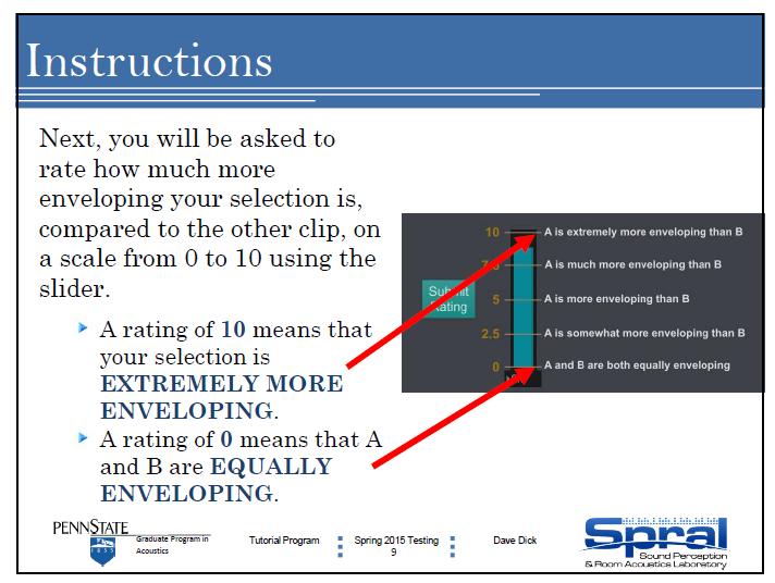
203 182

204 183

205 184

206 185

207 186

208 187

209 188