S2 series. Network Analyzer Operating Manual

Transcription

1 S2 series Network Analyzer Operating Manual Software Version

2 T A B L E O F C O N T E N T S INTRODUCTION... 8 SAFETY INSTRUCTIONS... 9 SCOPE OF MANUAL GENERAL OVERVIEW Description Specifications Measurement Capabilities Principle of Operation PREPARATION FOR USE General Information Software Installation Front Panel Power Switch Test Ports Ground Terminal Adjustable ports configurations (Planar 814/1 only) Rear Panel Power Cable Receptacle External Trigger Signal Input Connector External Trigger Signal Output Connector (Cobalt models only) External Reference Frequency Input Connector (Planar and Cobalt models) Internal Reference Frequency Output Connector (Planar and Cobalt models) Reference Frequency Input/Output Connector (S models) USB 2.0 High Speed Reserved Port (Planar 304/1) Auxiliary input ports (Cobalt models only) Fuse Holder (С1209 only) Ground terminal GETTING STARTED Analyzer Preparation for Reflection Measurement Analyzer Presetting Stimulus Setting IF Bandwidth Setting Number of Traces, Measured Parameter and Display Format Setting Trace Scale Setting

3 TABLE OF CONTENTS 3.7 Analyzer Calibration for Reflection Coefficient Measurement SWR and Reflection Coefficient Phase Analysis Using Markers SETTING MEASUREMENT CONDITIONS Screen Layout and Functions Softkey Menu Bar Menu Bar Instrument Status Bar Channel Window Layout and Functions Channel Title Bar Trace Status Field Graph Area Trace Layout in Channel Window Markers Channel Status Bar Quick Channel Setting Using a Mouse Active Channel Selection Active Trace Selection Measured Data Setting Display Format Setting Trace Scale Setting Reference Level Setting Reference Level Position Sweep Start Setting Sweep Stop Setting Sweep Center Setting Sweep Span Setting Marker Stimulus Value Setting Switching between Start/Center and Stop/Span Modes Start/Center Value Setting Stop/Span Value Setting Sweep Points Number Setting Sweep Type Setting IF Bandwidth Setting Power Level / CW Frequency Setting Channel and Trace Display Setting Channel Allocation Number of Traces Trace Allocation Selection of Active Trace/Channel Active Trace/Channel Window Maximizing Stimulus Setting Sweep Type Setting Sweep Span Setting Sweep Points Setting Stimulus Power Setting Setting Power Level for Each Port Individually

4 TABLE OF CONTENTS Power Slope Feature CW Frequency Setting RF Out Function Segment Table Editing Measurement Delay Trigger Setting External Trigger (except Planar 304/1) Trigger Output (Cobalt models) Measurement Parameters Setting S-Parameters S-Parameter Setting Absolute Measurements Absolute Measurement Setting Format Setting Rectangular Formats Polar Format Smith Chart Format Data Format Setting Scale Setting Rectangular Scale Rectangular Scale Setting Circular Scale Circular Scale Setting Automatic Scaling Reference Level Automatic Selection Electrical Delay Setting Phase Offset Setting Measurement Optimization IF Bandwidth Setting Averaging Setting Smoothing Setting Mixer Measurements Mixer Measurement Methods Frequency Offset Mode Source/Receivers Frequency Offset Feature Automatic Adjustment of Offset Frequency CALIBRATION AND CALIBRATION KIT General Information Measurement Errors Systematic Errors Error Modeling Analyzer Test Port Definition Calibration Steps Calibration Methods Calibration Standards and Calibration Kits

5 TABLE OF CONTENTS 5.2 Calibration Procedures Calibration Kit Selection Reflection Normalization Transmission Normalization Full One-Port Calibration One-Path Two-Port Calibration Full Two-Port Calibration TRL Calibration (except Planar 304/1) Calibration Using Subclasses Calibration Using Sliding Load Error Correction Disabling Error Correction Status System Impedance Z Port Extension Automatic Port Extension Non-Insertable Device Measuring Calibration Kit Management Table of Calibration Kits Calibration Standard Definition Table of Calibration Standard S-Parameters Calibration Standard Class Assignment Power Calibration Loss Compensation Table Power Calibration Procedure Power Correction Setting Loss Compensation Table Editing Receiver Calibration Receiver Calibration Procedure Receiver Correction Setting Scalar Mixer Calibration Vector Mixer Calibration Vector Mixer Calibration Procedure Automatic Calibration Module Automatic Calibration Module Features Automatic Calibration Procedure User Characterization Procedure Confidence Check Procedure Erasing the User Characterization MEASUREMENT DATA ANALYSIS Markers Marker Adding Marker Deleting Marker Stimulus Value Setting Marker Activating Reference Marker Feature

6 TABLE OF CONTENTS Marker Properties Marker Position Search Functions Marker Math Functions Marker Functions Memory Trace Function Saving Trace into Memory Trace Display Setting Mathematical Operations Fixture Simulation Port Z Conversion De-embedding Embedding Time Domain Transformation Time Domain Transformation Activating Time Domain Transformation Span Time Domain Transformation Type Time Domain Transformation Window Shape Setting Frequency Harmonic Grid Setting Time Domain Gating Time Domain Gate Activating Time Domain Gate Span Time Domain Gate Type Time Domain Gate Shape Setting S-Parameter Conversion General S-Parameter Conversion Limit Test Limit Line Editing Limit Test Enabling/Disabling Limit Test Display Management Limit Line Offset Ripple Limit Test Ripple Limit Editing Ripple Limit Enabling/Disabling Ripple Limit Test Display Management ANALYZER DATA OUTPUT Analyzer State Analyzer State Saving Analyzer State Recalling Session Saving Channel State Channel State Saving Channel State Recalling Trace Data CSV File

7 TABLE OF CONTENTS CSV File Saving/Recalling Trace Data Touchstone File Touchstone File Saving/Recalling SYSTEM SETTINGS Analyzer Presetting Graph Printing Reference Frequency Oscillator Selection System Correction Setting Beeper Setting User Interface Setting Screen Update Setting Power Meter Setting Port Overload Indication (expect Planar 304/1) Power Trip Function (expect Planar 304/1) Port Switchover Delay Disabling Direct receiver access (for C2220 only) MAINTENANCE AND STORAGE Maintenance Procedures Instrument Cleaning Factory Calibration Performance Test Storage Instructions Appendix 1 Default Settings Table

8 INTRODUCTION This Operating Manual contains design, specifications, functional overview, and detailed operation procedures for the Network Analyzer, to ensure effective and safe use of its technical capabilities by the user. Maintenance and operation of the Analyzer should be performed by qualified engineers with basic experience in operating of microwave circuits and PC. The following abbreviations are used in this Manual: PC DUT IF CW Personal Computer Device Under Test Intermediate Frequency Continuous Wave SWR Standing Wave Ratio CMT Copper Mountain Technologies 8

9 SAFETY INSTRUCTIONS Carefully read the following safety instructions before putting the Analyzer into operation. Observe all the precautions and warnings provided in this Manual for all the phases of operation, service, and repair of the Analyzer. The Analyzer should be used only by skilled and thoroughly trained personnel with the required skills and knowledge of safety precautions. The Analyzer complies with INSTALLATION CATEGORY II as well as POLLUTION DEGREE 2 as defined in IEC The Analyzer is a MEASUREMENT CATEGORY I (CAT I) device. Do not use the Analyzer as a CAT II, III, or IV device. The Analyzer is for INDOOR USE only. The Analyzer has been tested as a stand-alone device and in combination with the accessories supplied by Copper Mountain Technologies, in accordance with the requirements of the standards described in the Declaration of Conformity. If the Analyzer is integrated with another system, compliance with related regulations and safety requirements are to be confirmed by the builder of the system. Never operate the Analyzer in an environment containing flammable gasses or fumes. Operators must not remove the cover or any other part of the housing. The Analyzer must not be repaired by the operator. Component replacement or internal adjustment must be performed by qualified maintenance personnel only. Never operate the Analyzer if the power cable is damaged. Never connect the test ports to A/C power mains. Electrostatic discharge can damage the Analyzer whether connected to or disconnected from the DUT. Static charge can build up on your body and damage sensitive internal components of both the Analyzer and the DUT. To avoid damage from electric discharge, observe the following: Always use a desktop anti-static mat under the DUT. Always wear a grounding wrist strap connected to the desktop anti-static mat via daisy-chained 1 MΩ resistor. Connect the post marked on the body of the Analyzer to the body of the DUT before you start operation. Observe all general safety precautions related to operation of electrically energized equipment. 9

10 SAFETY INSTRUCTIONS The definitions of safety symbols used on the instrument and in the Manual are listed below. Refers to the Manual if the instrument is marked with this symbol. Alternating current. Direct current. On (Supply). Off (Supply). A chassis terminal; a connection to the instrument s chassis, which includes all exposed metal surfaces. WARNING CAUTION Note This sign denotes a hazard. It calls attention to a procedure, practice, or condition that, if not correctly performed or adhered to, could result in injury or death to personnel. This sign denotes a hazard. It calls attention to a procedure, practice, or condition that, if not correctly performed or adhered to, could result in damage to or destruction of part or all of the instrument. This sign denotes important information. It calls attention to a procedure, practice, or condition that is essential for the user to understand. 10

11 SAFETY INSTRUCTIONS SCOPE OF MANUAL This manual covers the 2-port models of the CMT network analyzers controlled by the S2VNA software. The analyzer models are listed below. Planar 304/1 Planar 804/1 Planar 814/1 S5048 S5065 S5085 S7530 S5180 C1209 C1220 C2220 C2209 C4209 C

12 1 GENERAL OVERVIEW 1.1 Description The Analyzer is designed for use in the process of development, adjustment and testing of various electronic devices in industrial and laboratory facilities, including operation as a component of an automated measurement system. The Analyzer is designed for operation with an external PC, which is not supplied with the Analyzer. 1.2 Specifications The specifications of each Analyzer model can be found in its corresponding datasheet. 1.3 Measurement Capabilities Measured parameters S 11, S 21, S 12, S 22 Number of measurement channels Data traces Memory traces Data display formats Absolute power of the reference and received signals at the port. Up to 16 logical channels. Each logical channel is represented on the screen as an individual channel window. A logical channel is defined by such stimulus signal settings as frequency range, number of test points, power level, etc. Up to 16 data traces can be displayed in each channel window. A data trace represents one of the following parameters of the DUT: S- parameters, response in the time domain, or input power response. Each of the 16 data traces can be saved into memory for further comparison with the current values. Logarithmic magnitude, linear magnitude, phase, expanded phase, group delay, SWR, real part, imaginary part, Smith chart format and polar format. 12

13 1 GENERAL OVERVIEW Sweep setup features Sweep type Measured points per sweep Segment sweep Power settings Sweep trigger Linear frequency sweep, logarithmic frequency sweep, and segment frequency sweep, when the stimulus power is a fixed value; and linear power sweep when frequency is a fixed value. From 2 to the instrument maximum. A frequency sweep within several user-defined segments. Frequency range, number of sweep points, source power, and IF bandwidth can be set for each segment. Source power from instrument minimum to instrument maximum with resolution of 0.05 db. In frequency sweep mode the power slope can be set to up to 2 db/ghz to compensate high frequency attenuation in cables. Trigger modes: continuous, single, hold. Trigger sources: internal, manual, external, bus. Trace display functions Trace display Trace math Data trace, memory trace, or simultaneous data and memory traces. Data trace modification by math operations: addition, subtraction, multiplication or division of measured complex values and memory data. Autoscaling Automatic selection of scale division and reference level value to have the trace most effectively displayed. Electrical delay Phase offset Calibration plane compensation for delay in the test setup, or for electrical delay in a DUT during measurements of deviation from linear phase. Phase offset in degrees. 13

14 1 GENERAL OVERVIEW Accuracy enhancement Calibration Calibration methods Calibration of a test setup (which includes the Analyzer, cables, and adapters) significantly increases the accuracy of measurements. Calibration allows for correction of errors caused by imperfections in the measurement system: system directivity, source and load match, tracking, and isolation. The following calibration methods of various sophistication and accuracy enhancement are available: reflection and transmission normalization; full one-port calibration; one-path two-port calibration full two-port calibration; TRL calibration (except Planar 304/1). Reflection and transmission normalization Full one-port calibration One-path two-port calibration Full two-port calibration TRL calibration (except Planar 304/1) The simplest calibration method. It provides limited accuracy. Method of calibration performed for one-port reflection measurements. It ensures high accuracy. Method of calibration performed for reflection and one-way transmission measurements, for example for measuring S 11 and S 21 only. It ensures high accuracy for reflection measurements, and reasonable accuracy for transmission measurements. Method of calibration performed for full S-parameter matrix measurement of a two-port DUT. It ensures high accuracy. Method of calibration performed for full S-parameter matrix measurement of a two-port DUT. LRL and LRM types of this calibration are also supported. In ensures higher accuracy than a two-port calibration. 14

15 1 GENERAL OVERVIEW Mechanical calibration kits Electronic calibration modules Sliding load calibration standard Unknown thru calibration standard (except Planar 304/1) Defining of calibration standards The user can select one of the predefined calibration kits of various manufacturers or define additional calibration kits. Copper Mountain Technologies automatic calibration modules make the Analyzer calibration faster and easier than traditional mechanical calibration. The use of sliding load calibration standard allows significant increase in calibration accuracy at high frequencies compared to a fixed load calibration standard. The use of an arbitrary reciprocal two-port device instead of a zero-length thru during a full twoport calibration allows for calibration of the test setup for measurements of non-insertable devices. Different methods of calibration standard definition are available: standard definition by polynomial model standard definition by data (S-parameters). Error correction interpolation When the user changes such settings as start/stop frequencies and number of sweep points, compared to the settings of calibration, interpolation or extrapolation of the calibration coefficients will be applied. Supplemental calibration methods Power calibration Method of calibration which allows for maintaining more stable power levels at the DUT input. An external power meter should be connected to the USB port directly or via USB/GPIB adapter. Receiver calibration Method of calibration which calibrates the receiver gain at absolute signal power measurement. 15

16 1 GENERAL OVERVIEW Marker functions Data markers Reference marker Marker search Marker search additional features Setting parameters by markers Marker math functions Up to 16 markers for each trace. A marker indicates the stimulus value and measurement result at a given point of the trace. Enables indication of any maker value as relative to the reference marker. Search for max, min, peak, or target values on a trace. User-definable search range. Available as either a tracking marker, or as a one-time search. Setting of start, stop and center frequencies from the marker frequency, and setting of reference level by the measurement result of the marker. Statistics, bandwidth, flatness, RF filter. Statistics Calculation and display of mean, standard deviation and peak-to-peak in a frequency range limited by two markers on a trace. Bandwidth Flatness RF filter Determines bandwidth between cutoff frequency points for an active marker or absolute maximum. The bandwidth value, center frequency, lower frequency, higher frequency, Q value, and insertion loss are displayed. Displays gain, slope, and flatness between two markers on a trace. Displays insertion loss and peak-to-peak ripple of the passband, and the maximum signal magnitude in the stopband. The passband and stopband are defined by two pairs of markers. 16

17 1 GENERAL OVERVIEW Data analysis Port impedance conversion De-embedding Embedding S-parameter conversion Time domain transformation Time domain gating The function converts S-parameters measured at the analyzer s nominal port impedance into values which would be found if measured at a test port with arbitrary impedance. The function allows mathematical exclusion of the effects of the fixture circuit connected between the calibration plane and the DUT. This circuit should be described by an S-parameter matrix in a Touchstone file. The function allows mathematical simulation of the DUT parameters after virtual integration of a fixture circuit between the calibration plane and the DUT. This circuit should be described by an S- parameter matrix in a Touchstone file. The function allows conversion of the measured S- parameters to the following parameters: reflection impedance and admittance, transmission impedance and admittance, and inverse S- parameters. The function performs data transformation from frequency domain into response of the DUT to various stimulus types in time domain. Modeled stimulus types: bandpass, lowpass impulse, and lowpass step. Time domain span is set by the user arbitrarily from zero to maximum, which is determined by the frequency step. Various window shapes allow optimizing the tradeoff between resolution and level of spurious sidelobes. The function mathematically removes unwanted responses in time domain, allowing for obtaining frequency response without the influence of the fixture elements. The function applies a reverse transformation back to the frequency domain from the user-defined span in the time domain. Gating filter types: bandpass or notch. For better tradeoff between gate resolution and level of spurious sidelobes the following filter shapes are available: maximum, wide, normal and minimum. 17

18 1 GENERAL OVERVIEW Mixer / converter measurements Scalar mixer / converter The scalar method allows measurement of scalar transmission S-parameters of mixers and other measurements devices having different input and output frequencies. No external mixers or other devices are required. The scalar method employs port frequency offset when there is a difference between receiver frequency and source frequency. Vector mixer / converter measurements Scalar mixer / converter calibration Vector mixer /converter calibration Automatic adjustment of frequency offset The vector method allows measuring of the mixer transmission S-parameter magnitude and phase. The method requires an external mixer and an LO common to both the external mixer and the mixer under test. The most accurate method of calibration applied for measurements of mixers in frequency offset mode. The OPEN, SHORT, and LOAD calibration standards are used. An external power meter should be connected to the USB port directly or via USB/GPIB adapter. Method of calibration applied for vector mixer measurements. The OPEN, SHORT and LOAD calibration standards are used. The function performs automatic frequency offset adjustment when scalar mixer / converter measurements are performed to compensate for LO frequency inaccuracies internal to the DUT. Other features Familiar graphical user interface Analyzer control Printout/saving of traces Graphical user interface based on the Windows operating system ensures fast and easy Analyzer operation by the user. Using a personal computer. The traces and data printout function has a preview feature. Previewing, saving and printing can be performed using MS Word, Image Viewer for Windows, or the Analyzer Print Wizard. 18

19 1 GENERAL OVERVIEW Remote control COM/DCOM SCPI Remote control via COM/DCOM. COM automation runs the user program on an Analyzer PC. DCOM automation runs the user program on a LANnetworked PC. Automation of the instrument can be achieved in any COM/DCOM-compatible language or environment, including Python, C++, C#, VB.NET, LabVIEW, MATLAB, Ocatve, VEE, Visual Basic (Excel) and others. Remote control using textual commands SCPI (Standard Commands for Programmable Instruments). The text messages are delivered over computer networks using HiSLIP or TCP/IP Socket network protocols. The VISA library supports both protocols. The VISA library is a widely used software input-output interface in the field of testing and measurement for controlling devices from a personal computer. It is a library of functions for C/C ++, C #, Visual Basic, MATLAB, LabVIEW and others. 19

20 1 GENERAL OVERVIEW 1.4 Principle of Operation The block diagram of the Analyzer is represented in Figure 1. The Analyzer Unit consists of a source oscillator, local oscillator, source power attenuator, and a switch connecting the source signal to two directional couplers, which are connected to the Port 1 and Port 2 connectors. The incident and reflected waves from the directional couplers are passed into the mixers, where they are converted to first IF (10.7 MHz for Planar models; 0.4 MHz for S models; 7.6 MHz for Cobalt models) and are passed further to the 4-Channel receiver. The 4-Channel receiver, after filtering, digitally encodes the signal and supplies it for further processing (filtration, phase difference estimation, magnitude measurement) by the signal processor. The IF measurement filters are digital and have bandwidths of between the instrument minimum (1 Hz for Planar and Cobalt models; 10 Hz for S models) to instrument maximum (30 khz for Planar and S models; 1MHz for Cobalt models). Either port of the Analyzer can be a source of the tested signal as well as a receiver of the signal transferred thought the DUT. If Port 1 is a source, Port 2 will be a receiver. The definition incident and reflected wave is correct for the port when it is a source of the test signal. The combination of the assemblies of directional couplers, mixers and 4-Channel receiver forms four similar signal receivers. An external PC controls the operation of the components of the Analyzer. To perform S-parameter measurements, the Analyzer supplies the source signal of the assigned frequency from one of the ports to the DUT, then measures magnitude and phase of the signals transmitted through and reflected by the DUT, and finally compares these results to the magnitude and phase of the source signal. 20

21 1 GENERAL OVERVIEW Figure 1 Analyzer Block Diagram 21

22 1 GENERAL OVERVIEW Planar 814/1 has adjustable ports configurations with direct access to the receivers. This adjustable port configuration with direct access to the receivers of the VNA provides for a variety of test applications requiring wider dynamic and power range. Direct receiver access enables testing of high power devices. Additional amplifiers, attenuators, various filters and matching pads for each of the ports can be introduced in reference oscillator and receiver path to ensure the optimal operation mode of the receivers and the DUT, close to the real. Figure 2 Adjustable port configuration with direct access to the receivers 22

23 2 PREPARATION FOR USE 2.1 General Information Unpack the Analyzer and other accessories. Connect the Analyzer to a 100 VAC to 240 VAC 50/60 Hz power source by means of the external Power Supply (S models models) or Power Cable (Planar and Cobalt models) supplied with the instrument. Connect the USB-port of your Analyzer to the PC using the USB Cable supplied in the package. Install the software from onto your PC. The software installation procedure is described in section 2.2. Warm up the Analyzer for the time stated in its specifications. Assemble the test setup using cables, connectors, fixtures, etc., which allow DUT connection to the Analyzer. Perform calibration of the Analyzer. Calibration procedures are described in section Software Installation Connect the Analyzer to your PC via USB interface and install the Analyzer software from Minimal system requirements for the PC WINDOWS XP/VISTA/7/8/ GHz Processor 1 GB RAM USB 2.0 High Speed 23

24 2 PREPARATION FOR USE Program and other files installation Driver installation Run the Setup_S2VNA_vX.X.exe installer file. Follow the instructions of the installation wizard. Connect the Analyzer to your PC via the supplied USB cable. It is allowed to connect the USB cable to the running PC. Turn on and boot the PC, if it is off. Turn the Analyzer on by the Power key on the front panel. When you connect the Analyzer to the PC for the first time, Windows will automatically detect the new USB device and install the drivers automatically. Should automatic driver installation fail, open the USB driver installation dialog as follows: Start > Control Panel > Device Manager. Make the right mouse click on the Unknown Device line and select Update Drivers. In the USB driver installation dialog, click on Browse and specify the path to the driver files, which are contained in the \DRIVER folder in the Analyzer s software folder. When the driver is installed, a new USB device (Network Analyzer) will appear in the system. 24

25 2 PREPARATION FOR USE 2.3 Front Panel The front view of the Analyzers are represented in the figures below. The front panel is equipped with the following parts: Power switch; Test ports; LED indicators; Ground terminal; Adjustable ports configurations (Planar 814/1 only). Figure 3 Planar 304/1 front panel 25

26 2 PREPARATION FOR USE Figure 4 Planar 804/1 front panel Figure 5 Planar 814/1 front panel Figure 6 S5048 front panel Figure 7 S7530 front panel 26

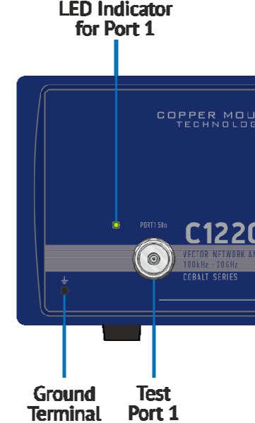
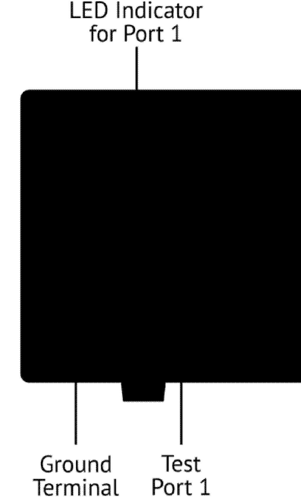
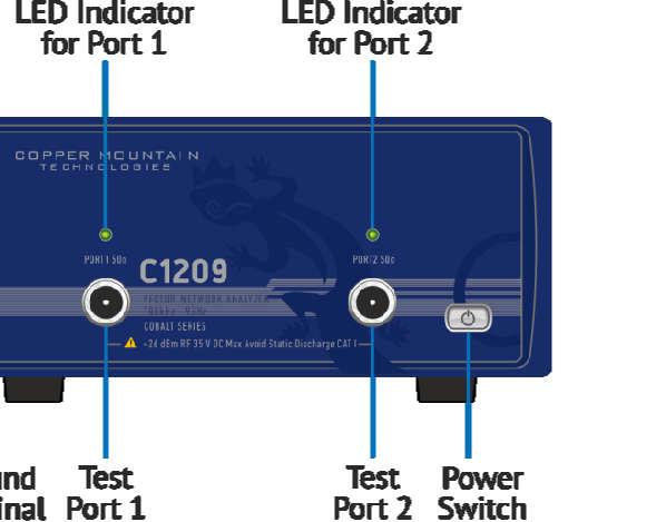
27 2 PREPARATION FOR USE Figure 8 C1209 front panel Figure 9 C1220 front panel 27

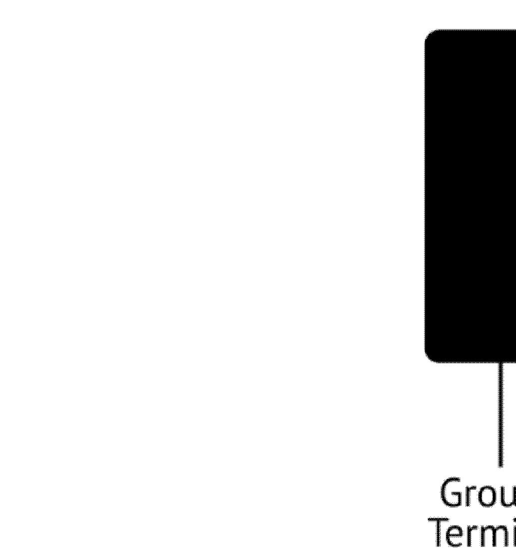
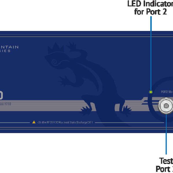
28 2 PREPARATION FOR USE Power Switch Switches the power supply of the Analyzer on and off. You can turn your Analyzer on/off at any time. After power-on of the Analyzer connected to PC, the program will begin downloading embedded firmware into the Analyzer. The process will take approximately 10 seconds, after which the Analyzer will be ready for operation. Note When you turn on your Analyzer for the first time, the USB driver will be installed onto the PC. The driver installation procedure is described in section 2.2. Some computers may require re-installation of the driver in case of change of the USB port Test Ports The Port 1 and test Port 2 are intended for DUT connection. Planar and S models and C1209 have type-n female test ports. C1220 has NMD 3.5 mm male test ports. Each test port has a LED indicator. A test port can be used either as a source of the stimulus signal or as a receiver of the response signal of the DUT. Only one of the ports can be the source of the signal at a particular moment of time. If you connect the DUT to only one test port of the Analyzer, you will be able to measure the reflection parameters (e.g. S 11 or S 22) of the DUT. If you connect the DUT to all test ports of the Analyzer, you will be able to measure the full S- parameter matrix of the DUT. Note LED indicator identifies the test port which is operating as a signal source. 28

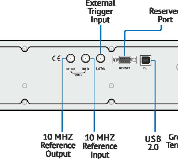
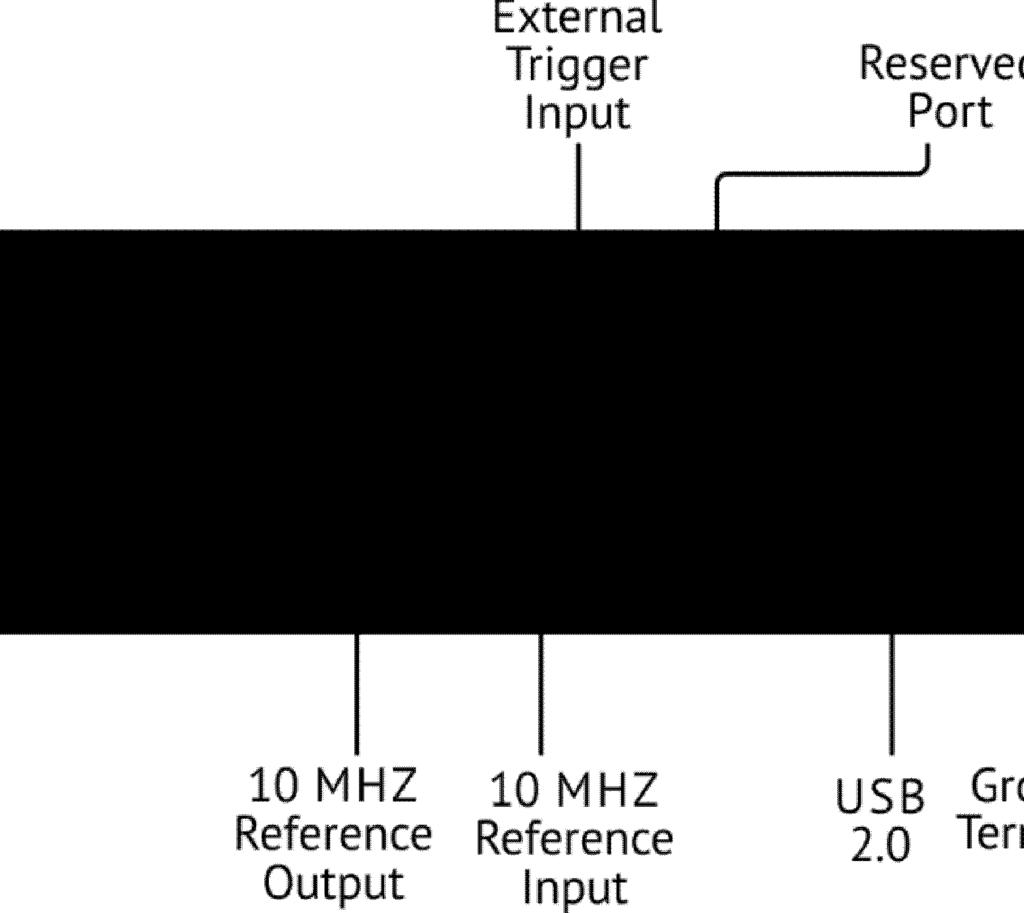
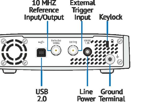
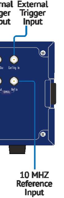
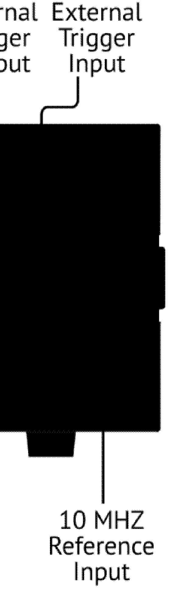
29 2 PREPARATION FOR USE CAUTION Do not exceed the maximum allowed power of the input RF signal (or maximum DC voltage) indicated on the front panel. This may damage your Analyzer Ground Terminal Use the terminal for grounding. To avoid damage from electric discharge, connect ground terminal on the body of the Analyzer to the body of the DUT Adjustable ports configurations (Planar 814/1 only) Adjustable ports configurations with direct access to the receivers of the VNA provides for a variety of test applications requiring wider dynamic and power range. Direct receiver access enables testing of high power devices. Additional amplifiers, attenuators, various filters and matching pads for each of the ports can be introduced in reference oscillator and receiver path to ensure the optimal operation mode of the receivers and the DUT, close to the real. 2.4 Rear Panel The rear view of the Analyzers are represented in the figures below. The rear panel is equipped with the following parts: Power cable or power supply receptacle; External trigger input connector; External trigger output connector (Cobalt models only); Reference Frequency input connector; Reference Frequency output connector; USB 2.0 High Speed receptacle; Reserved port (Planar 304/1 only); 29

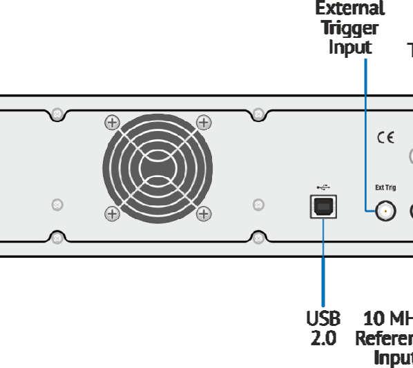
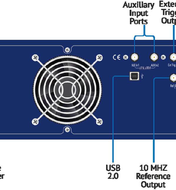
30 2 PREPARATION FOR USE Auxiliary input ports (Cobalt models only); Fuse Holder (C1209 only); Ground terminal. Figure 10 Planar 304/1 rear panel Figure 11 Planar 804/1 rear panel 30

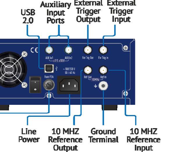
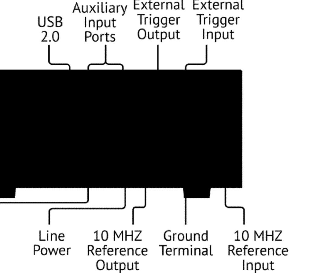
31 2 PREPARATION FOR USE Figure 12 S models rear panel Figure 13 C1209 rear panel Figure 14 C1220 rear panel 31

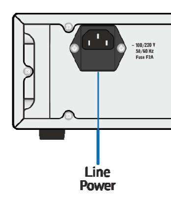
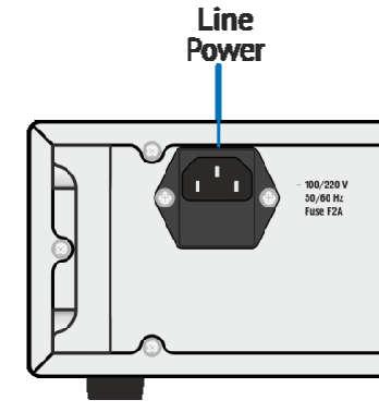
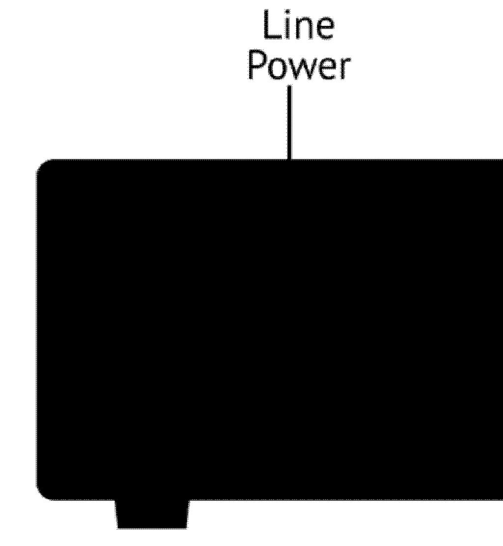
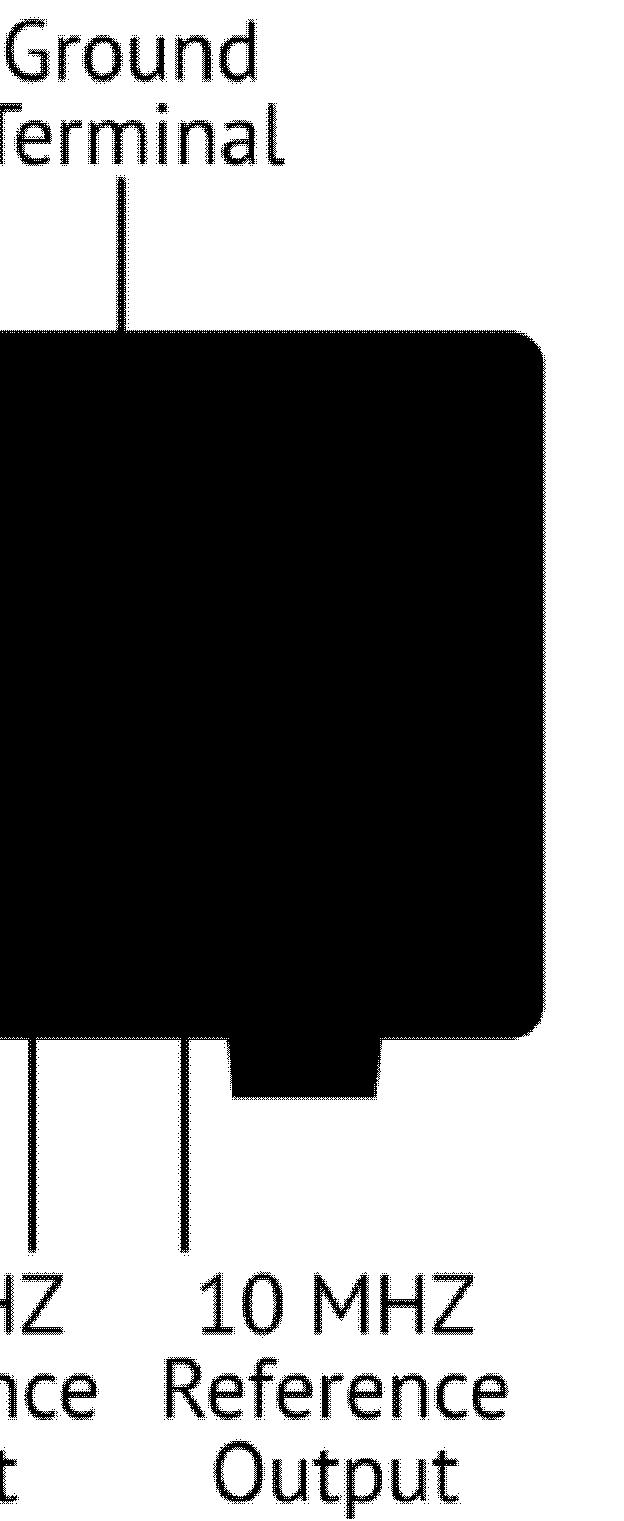
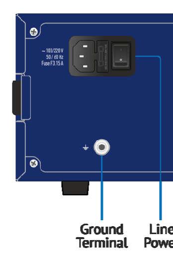
32 2 PREPARATION FOR USE Power Cable Receptacle The power cable receptacle (Planar and Cobalt models) is intended for 100 VAC to 240 VAC 50/60 Hz power cable connection. The power supply receptacle (S models) is intended for an external DC power supply voltage from 9 to 15 V; alternatively the power supply can be powered by a battery, including a vehicle battery, through an appropriate vehicle power cable External Trigger Signal Input Connector This connector allows the user to connect an external trigger source. Connector type is BNC female. Planar and S models TTL compatible inputs of 3 V to 5 V magnitude have up to 1 µs pulse width. Input impedance at least 10 kω. Cobalt models TTL compatible inputs of 0 V to 5 V magnitude have up to 2 µs pulse width. Input impedance at least 10 kω External Trigger Signal Output Connector (Cobalt models only) The External Trigger Signal Output port can be used to provide trigger to an external device. The port outputs various waveforms depending on the setting of the Output Trigger Function: before frequency setup pulse, before sampling pulse, after sampling pulse, ready for external trigger, end of sweep pulse, measurement sweep External Reference Frequency Input Connector (Planar and Cobalt models) External reference frequency is 10 MHz, input level is 2 dbm ± 2 db, input impedance at «Ref In» is 50 Ω. Connector type is BNC female. 32

33 2 PREPARATION FOR USE Internal Reference Frequency Output Connector (Planar and Cobalt models) Output reference signal level is 3 dbm ± 2 db at 50 Ω impedance. «Ref Out» connector type is BNC female Reference Frequency Input/Output Connector (S models) External reference frequency is 10 MHz, input level is 2 dbm ± 3 db, input impedance 50 Ω. Output reference signal level is 3 dbm ± 2 db into 50 Ω impedance. Connector type is BNC female USB 2.0 High Speed The USB port is intended for connection to a computer Reserved Port (Planar 304/1) Note Do not use this port Auxiliary input ports (Cobalt models only) Auxiliary input ports allow the user to input DC signal for DC signal measurement. This is useful in cases where the DUT works on a DC supply and it is required to measure the DC supply along with other measurements of the DUT using the Analyzer Fuse Holder (С1209 only) Fuse protects the Analyzer from the excessive current. 33

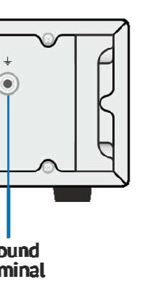
34 2 PREPARATION FOR USE Ground terminal To avoid electric shock, use the terminal for grounding. Ground terminal allows the user to directly connect the body of the Analyzer to the grounding bar in order to ensure electrical safety. 34

35 3 GETTING STARTED This section is organized as a sample session of the Analyzer. It describes the main techniques of measurement of reflection coefficient parameters of the DUT. SWR and reflection coefficient phase of the DUT will be analyzed. For reflection coefficient measurement only one test port of the Analyzer is used. The instrument sends the stimulus to the input of the DUT and then receives the reflected wave. Generally in the process of this measurement the output of the DUT should be terminated with a LOAD standard. The results of these measurements can be represented in various formats. Typical circuit of reflection coefficient measurement is shown in Figure 15. DUT Figure 15 Reflection measurement circuit To measure SWR and reflection coefficient phases of the DUT, in the given example you should go through the following steps: Prepare the Analyzer for reflection measurement; Set stimulus parameters (frequency range, number of sweep points); Set IF bandwidth; Set the number of traces to 2, assign measured parameters and display format to the traces; Set the scale of the traces; 35

36 3 GETTING STARTED Perform calibration of the Analyzer for reflection coefficient measurement; Analyze SWR and reflection coefficient phase using markers. Note In this section the control over Analyzer is performed by the softkeys located in the right-hand part of the screen. The Analyzer also allows the user to perform quick control by the mouse (See section 4.3). 3.1 Analyzer Preparation for Reflection Measurement Turn on the Analyzer and warm it up for the period of time stated in its specifications. Ready state features The bottom line of the screen displays the instrument status bar. It should read Ready. Above this bar, the channel status bar is located. The sweep indicator in the left-hand part of this bar should display a progress. Connect the DUT to Port 1 of the Analyzer. Use the appropriate cables and adapters for connection of the DUT input to the Analyzer test port. If the DUT input is type-n (male), you can connect the DUT directly to the port. 3.2 Analyzer Presetting Before you start the measurement session, it is recommended to reset the Analyzer into the initial (known) condition. The initial condition setting is described in Appendix 1. To restore the initial condition of the Analyzer, use the following softkeys: System > Preset > OK 36

37 3 GETTING STARTED 3.3 Stimulus Setting After you have restored the preset state of the Analyzer, the stimulus parameters will be as follows: full frequency range of the instrument, sweep type is linear, number of sweep points is 201, and power level is 0 dbm. For the current example, set the frequency range to from 10 MHz to 3 GHz. To set the start frequency of the frequency range to 10 MHz, use the following softkeys: Stimulus > Start Then enter «1», «0» from the keyboard. Complete the setting by pressing «M» key. To set the stop frequency of the frequency range to 3 GHz, use the following softkeys: Stimulus > Stop Then enter «3» from the keyboard. Complete the setting by pressing «G» key. To return to the main menu, click the top softkey (colored in blue). 3.4 IF Bandwidth Setting For the current example, set the IF bandwidth to 3 khz. To set the IF bandwidth to 3 khz, use the following softkeys: Average > IF Bandwidth Then enter «3» from the keyboard and complete the setting by pressing «k» key. To return to the main menu, click the top softkey (colored in blue). 37

38 3 GETTING STARTED 3.5 Number of Traces, Measured Parameter and Display Format Setting In the current example, two traces are used for simultaneous display of the two parameters (SWR and reflection coefficient phase). To set the number of traces, use the following softkeys: Display > Num of Traces > 2 To return to the main menu, click the top softkey (colored in blue). Before assigning the measurement parameters of a trace, first activate the trace. To activate the second trace, use the following softkeys: Display > Active Trace/Channel > Active Trace > 2 To return to the main menu, click the top softkey (colored in blue). Assign S 11-parameter to the second trace. To the first trace this parameter is already assigned by default. To assign a parameter to the trace, use the following softkeys: Measurement > S11 Then assign SWR display format to the first trace and reflection coefficient phase display format to the second trace. 38

39 3 GETTING STARTED To set the active trace display format, use the following softkeys: Format > SWR (for the first trace), Format > Phase (for the second trace). To return to the main menu, click the top softkey (colored in blue). 3.6 Trace Scale Setting For convenience of operation, change the trace scale using automatic scaling function. To set the scale of the active trace by the autoscaling function, use the following softkeys: Scale > Auto Scale To return to the main menu, click the top softkey (colored in blue). 3.7 Analyzer Calibration for Reflection Coefficient Measurement Calibration of the whole measurement setup which includes the Analyzer, cables and other devices involved with connection to the DUT allows for considerably enhancing the accuracy of the measurement. To perform full 1-port calibration, you need to prepare the kit of calibration standards: OPEN, SHORT and LOAD. Such a kit has its description and specifications of the standards. To perform proper calibration, you need to select the correct kit type in the program. To perform the process of full 1-port calibration, connect calibration standards to the test port one after another, as shown in Figure

40 3 GETTING STARTED LOAD OPEN SHORT Figure 16 Full 1-port calibration circuit In the current example, an Agilent 85032E calibration kit is used. To select the calibration kit, use the following softkeys: Calibration > Cal Kit Then select the kit you are using from the table at the bottom of the screen. To perform full 1-port calibration, you will execute measurements of the three standards in turn. After completion, the table of calibration coefficients will be calculated and saved into the memory of the Analyzer. Before you start calibration, disconnect the DUT from the Analyzer. 40

41 3 GETTING STARTED To perform full 1-port calibration, use the following softkeys: Calibration > Calibrate > Full 1-Port Cal Connect an OPEN standard and click Open. Connect a SHORT standard and click Short. Connect a LOAD standard and click Load. To complete the calibration procedure and calculate the table of calibration coefficients, click the Apply softkey. 3.8 SWR and Reflection Coefficient Phase Analysis Using Markers This section describes how to determine the measurement values at three frequency points using markers. The Analyzer screen view is shown in Figure 17. In the current example, a reflection standard of SWR = 1.2 is used as a DUT. Figure 17 SWR and reflection coefficient phase measurement example 41

42 3 GETTING STARTED To create a new marker, use the following softkeys: Markers > Add Marker Then enter the frequency value in the input field in the graph, e.g. to enter frequency 200 MHz, press «2», «0», «0» and «M» keys on the keypad. Repeat the above procedure three times to enable three markers at different frequency points. By default only active trace markers are displayed on the screen. To enable display of two traces simultaneously, activate the marker table. To open the marker table, use the following softkeys: Markers > Properties > Marker Table 42

43 4 SETTING MEASUREMENT CONDITIONS 4.1 Screen Layout and Functions The screen layout is represented in Figure 18. In this section you will find detailed descriptions of the softkey menu bar, menu bar, and instrument status bar. The channel windows are described elsewhere in this manual. Menu Softkey menu Channel window Instrument status Figure 18 Analyzer screen layout Softkey Menu Bar The softkey menu bar along the right side of the screen is the main menu of the program. Note The top line of the screen contains the menu bar, which provides direct access to certain submenus of the softkey menu. This is a secondary menu which can optionally be hidden. 43

44 4 SETTING MEASUREMENT CONDITIONS The softkey menu bar consists of a series of panels. Each panel represents one of the submenus of the softkey menu. All the panels are integrated to form the complete multilevel menu system, providing access to all the Analyzer functions. You can navigate the menu softkeys using a mouse. Alternatively you can navigate the menu using the,,,, «Enter», «Esc», and «Home» keys on an external keyboard. The types of softkeys are described below: The top softkey is the menu title key. It enables you to return to a higher level of the menu. If it is displayed in blue, you can use the keyboard to navigate within the softkey menu. If the softkey is highlighted in dark gray, pressing «Enter» key on the keyboard will activate the function of this softkey. You can shift the highlight from key to key using and arrows on the keyboard. A large dot on the softkey indicates the current selection in a list of alternative settings. A check mark in the left part of the softkey indicates an active function, which you can switch on/off. Softkeys with right arrows provide access to a lower level menu. A softkey with a text field allows for the selected function indication. Softkeys with a value field allow for entering/selection of the numerical settings. This navigation softkey appears when the softkey menu overflows the menu screen area. Using this softkey you can scroll down and up the softkey menu. 44

45 4 SETTING MEASUREMENT CONDITIONS To navigate in the softkey menu, you can also (additionally to, ) use,, «Esc», «Home» keys of the keyboard: key brings up the upper level of the menu; key brings up the lower level of the menu, if there is a highlighted softkey with a right arrow; «Esc» key functions similarly to the key; «Home» key brings up the main menu. Note The above keys of the keyboard allow navigation within the softkey menu only if there is no active entry field. In this case the menu title softkey is highlighted in blue Menu Bar Figure 19 Menu bar The menu bar is located at the top of the screen. This is a secondary menu providing direct access to certain submenus of the main menu. It also contains the most frequently used softkeys functions. You can optionally hide the menu bar to gain more screen space for the graph area. The menu bar is controlled by mouse. Note To hide the menu bar, use the following softkeys: Display > Properties > Menu Bar 45

46 4 SETTING MEASUREMENT CONDITIONS Instrument Status Bar Date and time Messages Figure 20 Instrument status bar The instrument status bar is located at the bottom of the screen. Table 1 Messages in the instrument status bar Field Description Message Instrument Status DSP status Sweep status Not Ready Loading Ready Meas Hold Ext Man Bus No communication between DSP and computer. DSP program is loading. DSP is running normally. A sweep is in progress. A sweep is on hold. Waiting for External trigger. Waiting for Manual trigger. Waiting for Bus trigger. Calibration Calibration Calibration standard measurement is in progress. RF signal RF output Off Stimulus signal output is turned off. External reference frequency ExtRef External reference frequency input (10 MHz) is turned on. Display update Update Off Display update is turned off. System correction status Factory calibration error External power meter status Sys Corr OFF PC Error RC Error Power Meter: message System correction is turned off (see section 8.4). ROM error of power calibration. ROM error of system calibration. When external power meter is connected to the Analyzer via USB the following 46

47 4 SETTING MEASUREMENT CONDITIONS messages are displayed: connection, connection error, ready, measurement, zero setting, zero setting error 4.2 Channel Window Layout and Functions The channel windows display measurement results in the form of traces and numerical values. The screen can display up to 16 channel windows simultaneously. Each window corresponds to one logical channel. A logical channel can be considered to be a separate analyzer with the following settings: Stimulus signal settings (frequency range, power level, sweep type); IF bandwidth and averaging; Calibration. The physical analyzer processes the logical channels sequentially. In turn, each channel window can display up to 16 trace of measured parameters. The general view of the channel window is represented in Figure 21. Figure 21 Channel window 47

48 4 SETTING MEASUREMENT CONDITIONS Channel Title Bar The channel title feature allows you to enter your comment for each channel window. You can hide the channel title bar to gain more screen space for graph area. Channel title bar on/off switching To show/hide the channel title bar, use the following softkeys: Display > Title Label Channel title editing You can access the channel title edit mode by using the following softkeys: Display > Edit Title Label Alternatively, mouse click on the title area in the channel title bar. 48

49 4 SETTING MEASUREMENT CONDITIONS Trace Status Field Trace properties Reference level value Trace scale Display format Measured parameter Trace name Figure 22 Trace status field The trace status field displays the name and parameters of a trace. The number of lines in the field depends on the number of active traces in the channel. Note Using the trace status field you can easily modify the trace parameters using the mouse (as described in section 4.3). Each line contains the data of one trace of the channel: Trace name from «Tr1» to «Tr16». The active trace name is highlighted in an inverted color; Measured parameter: S11, S21, S12, S22, or absolute power value: A(n), B(n), R1(n), R2(n); Display format, e.g. «Log Mag»; Trace scale in measurement units per scale division, e.g. «10.0 db/»; Reference level value, e.g. «0.00 db», where is the symbol of the reference level; Trace status is indicated as symbols in square brackets (See Table 2). 49

50 4 SETTING MEASUREMENT CONDITIONS Table 2 Trace status symbols definition Status Symbols Definition Error Correction Other Calibrations Data Analysis Trace Display Math Operations RO RS RT OP F1 F2 SMC RC PC Z0 FD FE PExt No indication D&M M Off D+M D M D*M D/M OPEN response calibration SHORT response calibration THRU response calibration One-path 2-port calibration Full 1-port calibration Full 2-port and TRL calibration Scalar mixer calibration Receiver calibration Power calibration Port impedance conversion Fixture de-embedding Fixture embedding Port extension Data trace Data and memory traces Memory trace Data and memory traces off Data + Memory Data Memory Data * Memory Data / Memory Electrical Delay Del Electrical delay other than zero Smoothing Smo Trace smoothing Gating Gat Time domain gating Conversion Zr Zt Yr Yt Reflection impedance Transmission impedance Reflection admittance Transmission admittance 1/S S-parameter inversion Ztsh Ytsh Transmission-shunt impedance Transmission-shunt admittance 50

51 4 SETTING MEASUREMENT CONDITIONS Conj Conjugation 51

52 4 SETTING MEASUREMENT CONDITIONS Graph Area The graph area displays traces and numeric data. Vertical graticule label Marker Reference line position Statistics Current stimulus position Horizontal graticule label Figure 23 Graph area Trace number The graph area contains the following elements: Vertical graticule label displays the vertical axis numeric data for the active trace. You can set the display of data for all the traces or hide the vertical graticule label to gain more screen space for the trace display. Horizontal graticule label displays stimulus axis numeric data (frequency, power level or time). You can also hide the horizontal graticule label to gain more screen space for the trace display. Reference level position indicates the reference level position of the trace. Markers indicate the measured values at points along the active trace. You can simultaneous display of markers for all traces. Marker functions: statistics, bandwidth, flatness, RF filter. 52

53 4 SETTING MEASUREMENT CONDITIONS Trace number allows trace identification when printing in black and white. Current stimulus position indicator appears when sweep duration exceeds 1.5 sec. Note Using the graticule labels, you can easily modify all the trace parameters using the mouse (as described in section 4.3) Trace Layout in Channel Window If the number of the displayed traces is more than one, you can rearrange the traces to suit your preference. You can allocate all the traces to one graph (See Figure 23) or display of each trace in an individual graph (See Figure 24). Figure 24 Two traces in one channel window (sample) 53

54 4 SETTING MEASUREMENT CONDITIONS Markers The markers indicate the stimulus values and the measured values at selected points of the trace (See Figure 25). Marker data field Indicator on trace Indicator on stimulus axis Figure 25 Markers The markers are numbered from 1 to 15. The reference marker is indicated with an R symbol. The active marker is indicated in the following manners: its number is highlighted with inverse color, the indicator on the trace is located above the trace, and the stimulus indicator is fully colored. 54

55 4 SETTING MEASUREMENT CONDITIONS Channel Status Bar The channel status bar is located in the bottom part of the channel window. It contains the following elements: Averaging status (if enabled) Power level IF bandwidth Sweep type Stimulus stop Sweep points Stimulus start Fixture simulation (if enabled) Port extension (if enabled) Power correction (if enabled) Receiver correction (if enabled) Error correction Sweep progress Figure 26 Channel status bar Sweep progress field displays a progress bar when the channel data are being updated. Error correction field displays the integrated status of error correction for S-parameter traces. The values of this field are represented in Table 3. Receiver correction field displays the integrated status of receiver correction for absolute power measurement traces. The values of this field are represented in Table 4. Power correction field displays the integrated status of power correction for all the traces. The values of this field are represented in Table 5. Port extension field displays the integrated status of execution of this function for S-parameter traces. If the function is enabled for all the traces, you will see black characters on a gray 55

56 4 SETTING MEASUREMENT CONDITIONS background. If the function is enabled just for some of the traces, you will see white characters on a red background. Fixture simulation field displays the integrated status of execution of this function for S-parameter traces. Fixture simulation includes the following operations: Z0 conversion, embedding, and de-embedding. If the function is enabled for all the traces, you will see black characters on a gray background. If the function is enabled just for some of the traces, you will see white characters on a red background. Stimulus start field allows for display and entry of the start frequency or power, depending on the sweep type. This field can be switched to indication of stimulus center frequency, in this case the word Start will change to Center. Sweep points field allows for display and entry of the number of sweep points. The number of sweep points can be set from 2 to the instrument maximum. Sweep type field allows for display and selection of the sweep type. The values of this field are represented in Table 6. IF bandwidth field allows for display and setting of the IF bandwidth. The values can be set from the instrument minimum to 30 khz. Power level field allows for display and entry of the port output power. In power sweep mode the field switches to indication of CW frequency of the source. Averaging status field displays the averaging status if this function is enabled. The first number is the averaging current counter value, the second one is the averaging factor. Stimulus stop field allows for display and entry of the stop frequency or power, depending on the sweep type. This field can be switched to indication of stimulus span, in this case the word Stop will change to Span. 56

57 4 SETTING MEASUREMENT CONDITIONS Table 3 Error correction field Symbol Definition Note Cor Error correction is enabled. The stimulus settings are the same for the measurement and the calibration. C? Error correction is enabled. The stimulus settings are not the same for the measurement and the calibration. Interpolation is applied. C! Error correction is enabled. The stimulus settings are not the same for the measurement and the calibration. Extrapolation is applied. If the function is active for all the traces black characters on a gray background. If the function is active only for some of the traces (other traces are not calibrated) white characters on a red background. Off Error correction is turned off. For all the traces. White characters on a red --- No calibration data. No calibration was background. performed. Table 4 Receiver correction field Symbol Definition Note RC RC? RC! Receiver correction is enabled. The stimulus settings are the same for the measurement and the calibration. Receiver correction is enabled. The stimulus settings are not the same for the measurement and the calibration. Interpolation is applied. Receiver correction is enabled. The stimulus settings are not the same for the measurement and the calibration. Extrapolation is applied. If the function is active for all the traces black characters on a gray background. If the function is active only for some of the traces (other traces are not calibrated) white characters on a red background. 57

58 4 SETTING MEASUREMENT CONDITIONS Table 5 Power correction field Symbol Definition Note PC Power correction is enabled. The stimulus settings are the same for the measurement and the calibration. PC? Power correction is enabled. The stimulus settings are not the same for the measurement and the calibration. Interpolation is applied. PC! Power correction is enabled. The stimulus settings are not the same for the measurement and the calibration. Extrapolation is applied. If the function is active for all the traces black characters on a gray background. If the function is active only for some of the traces (other traces are not calibrated) white characters on a red background. Table 6 Sweep types Symbol Definition Lin Log Segm Pow Linear frequency sweep. Logarithmic frequency sweep. Segment frequency sweep. Power sweep. 58

59 4 SETTING MEASUREMENT CONDITIONS 4.3 Quick Channel Setting Using a Mouse This section describes mouse operations which enable you to set the channel parameters quickly and easily. In a channel window, when hovering over the field where a channel parameter can be modified, the mouse pointer will change its icon to indicate edit mode. In text and numerical fields, edit mode will be indicated by underline «underline» symbol appearance. Note The mouse operations described in this section will help you adjust the most frequently used settings. The complete set of channel functions can be accessed via the softkey menu Active Channel Selection You can select the active channel when two or more channel windows are open. The border line of the active window will be highlighted in a light color. To activate another window, click inside its area Active Trace Selection You can select the active trace if the active channel window contains two or more traces. The active trace name will be highlighted in inverted color. To activate a trace, click on the required trace status line, or on the trace curve or the trace marker Measured Data Setting To assign the measured parameters (S 11, S 21, S 12 or S 22) to a trace, click on the S- parameter name in the trace status line and select the required parameter in the dropdown menu Display Format Setting To select the trace display format, click on the display format name in the trace status line and select the desired format in the drop-down menu. 59

60 4 SETTING MEASUREMENT CONDITIONS Trace Scale Setting The trace scale, also known as the vertical scale division value, can be set by either of two methods. The first method: click on the trace scale field in the trace status line and enter the required numerical value. The second method: move the mouse pointer over the vertical scale until the pointer icon becomes as shown in the figure. The pointer should be placed in the top or bottom parts of the scale, at approximately 10% of the scale height from the top or bottom of the scale. Left click and drag away from the scale center to enlarge the scale, or toward the scale center to reduce the scale Reference Level Setting The value of the reference level, which is indicated on the vertical scale by the and symbols, can be set by either of two methods. The first method: click on the reference level field in the trace status line and enter the required numerical value. The second method: move the mouse pointer over the vertical scale until the pointer icon becomes as shown in the figure. The pointer should be placed in the center part of the scale. Left click and drag up to increase the reference level value, or down to reduce the value. 60

61 4 SETTING MEASUREMENT CONDITIONS Reference Level Position The reference level position, indicated on the vertical scale by and symbols, can be set in the following way. Locate the mouse pointer on a reference level symbol until it becomes as shown in the figure. Then drag and drop the reference level symbol to the desired position Sweep Start Setting Move the mouse pointer over the stimulus scale until it becomes as shown in the figure. The pointer should be placed in the left part of the scale, at approximately 10% of the scale length from the left. Left click and drag right to increase the sweep start value, or left to reduce the value Sweep Stop Setting Move the mouse pointer over the stimulus scale until it becomes as shown in the figure. The pointer should be placed in the right part of the scale, at approximately 10% of the scale length from the right. Left click and drag right to increase the sweep stop value, or left to reduce the value Sweep Center Setting Move the mouse pointer over the stimulus scale until it becomes as shown in the figure. The pointer should be placed in the center part of the scale. Left click and drag right to increase the sweep center value, or left to reduce the value. 61

62 4 SETTING MEASUREMENT CONDITIONS Sweep Span Setting Move the mouse pointer over the stimulus scale until it becomes as shown in the figure. The pointer should be placed in the center part of the scale, at approximately 20% of the scale length from the right Left click and drag to the right to increase the sweep span value, or to the left to reduce the value Marker Stimulus Value Setting The marker stimulus value can be set by either a click and drag operation, or by entering the value using numerical keys of the keyboard. To drag the marker, first move the mouse pointer on one of the marker indicators until it becomes as shown in the figures. To enter the numerical value of the stimulus, first activate its field by clicking it in the marker data line Switching between Start/Center and Stop/Span Modes To switch between the modes Start/Center and Stop/Span, click on the respective field of the channel status bar. Clicking the label Start changes it to Center, and the label Stop will change to Span. The layout of the stimulus scale will be changed correspondingly Start/Center Value Setting To enter the Start/Center values, activate the respective field in the channel status bar by clicking the numerical value Stop/Span Value Setting To enter the Stop/Span values, activate the respective field in the channel status bar by clicking the numerical value Sweep Points Number Setting To enter the number of sweep points, activate the respective field in the channel status bar by clicking the numerical value. 62

63 4 SETTING MEASUREMENT CONDITIONS Sweep Type Setting To set the sweep type, left click on the respective field in the channel status bar and select the required type in the dropdown menu IF Bandwidth Setting IF bandwidth can be set by selection in the drop-down menu or by entering the value using numerical keys of the keyboard. To activate the drop-down menu, right click on the IF bandwidth field in the channel status bar. To enter the IF bandwidth, activate the respective field in the channel status bar by left clicking Power Level / CW Frequency Setting To enter the Power Level/CW Frequency, activate the respective field in the channel status bar by clicking the numerical value. The parameter displayed in the field depends on the current sweep type: in frequency sweep mode you can enter the power level value, in power sweep mode you can enter the CW frequency value. 63

64 4 SETTING MEASUREMENT CONDITIONS 4.4 Channel and Trace Display Setting The Analyzer supports 16 channels, each of which allows for measurements with stimulus parameter settings different from the other channels. The parameters related to a logical channel are listed in Table Channel Allocation A channel is represented on the screen as an individual channel window. The screen can display from 1 to 16 channel windows simultaneously. By default one channel window opens. If you need to open two or more channel windows select one of the layouts shown below. To set the channel window layout, use the following softkeys: Display > Allocate Channels Then select the required number and layout of the channel windows in the menu. The available options of number and layout of the channel windows on the screen are as follows: In accordance with the layouts, the channel windows do not overlap each other. The channels open sequentially starting from the smaller numbers. Note For each open channel window, you should set the stimulus parameters, adjust other settings, and perform calibration. Before you change a channel parameter setting or perform calibration of a channel, you need to ensure the channel is selected as active. 64

65 4 SETTING MEASUREMENT CONDITIONS The measurements are executed for open channel windows sequentially. Measurements for any hidden channel windows are not performed Number of Traces Each channel window can contain up to 16 different traces. Each trace is assigned a measured parameter (S-parameter), display format and other parameters. The parameters related to a trace are listed in Table 8. Traces can be displayed in one graph, overlapping each other, or in separate graphs within a channel window. The trace settings are made in two steps: trace number and trace layout within the channel window. By default the channel window contains one trace. If you need to enable two or more traces, set the number of traces as described below. To set the number of the traces, use the following softkeys: Display > Num Of Traces Then select the number of traces from the menu. All traces are assigned individual names, which cannot be changed. The trace name contains its number. The trace names are as follows: Tr1, Tr2... Tr16. Each trace is assigned some initial settings: measured parameter, format, scale, and color, which can be modified by the user. The measured parameters of the first four traces default to the following values: S 11, S 21, S 12, S 22. After that the measurement defaults repeat in cycles. By default the display format for all the traces is set to logarithmic magnitude (db). The scale parameters by default are set as follows: division is set to 10 db, reference level value is set to 0 db, and the reference level position is in the middle of the graph. The trace color is determined by its number. You can change the color for all the traces having the same number. 65

66 4 SETTING MEASUREMENT CONDITIONS Note The full cycle of trace update depends on the S- parameters measured and the calibration method. For example, the full cycle might consist of a single sweep with either Port 1 or Port 2 as the source, or might include two successive sweeps, of Port 1 then of Port 2. To have two traces (S 11 and S 22) measured, two successive sweeps will be performed. Two successive sweeps are also performed when full 2- port calibration is employed, independently of the number of the traces and S-parameters measured Trace Allocation By default races are displayed overlapping one other in the channel window. If you wish to display the traces in separate graphs, set the number and layout of the graphs in the channel window as shown below. To allocate the traces in a channel window, use the following softkeys: Display > Allocate Traces Then select the desired number and layout of the separate trace graphs in the menu. The available options of number and layout of the trace graphs of one channel window are as shown in section Unlike channel windows, the number of traces and their allocation into a number of graphs can be set independently. If the number of traces and the number of graphs are equal, all the traces will be displayed separately, each in its individual graph. If the number of traces is greater than the number of graphs, traces will be assigned successively (beginning from the smallest trace number) to the number of available graphs. When all the graphs are utilized, the process will continue from the first graph (the following in succession traces will be added in the graphs). 66

67 4 SETTING MEASUREMENT CONDITIONS If the number of traces is smaller than the number of graphs, empty graphs will be displayed. If two or more traces are displayed in one graph, the vertical scale will be shown for the active trace. Note The Analyzer can optionally show vertical graticule labels for all the traces in the graph. By default this feature is disabled. For details see section 8.6. If two or more traces are displayed in one graph, markers data will be shown for the active trace. Note To display the marker data for all the traces simultaneously, there are two options: use the marker table feature (See section ) or deactivate identification of the active trace marker only, which is set by default (See section ). The stimulus axis is the same for all the traces of the channel, except for the case when time domain transformation is applied to some of the traces. In this case the displayed stimulus axis will correspond to the active trace. Table 7 Channel parameters N Parameter Description 1 Sweep Type 2 Sweep Range 3 Number of Sweep Points 4 Stimulus Power Level 5 Power Slope Feature 6 CW Frequency 7 Segment Sweep Table 8 Trigger Mode 9 IF Bandwidth 10 Averaging 11 Calibration 12 Fixture Simulator 67

68 4 SETTING MEASUREMENT CONDITIONS Table 8 Trace parameters N Parameter Description 1 Measured Parameter (S parameter) 2 Display Format 3 Reference Level Scale, Value and Position 4 Electrical Delay, Phase Offset 5 Memory Trace, Math Operation 6 Smoothing 7 Markers 8 Time Domain 9 Parameter Transformation 10 Limit Test 68

69 4 SETTING MEASUREMENT CONDITIONS Selection of Active Trace/Channel The control commands selected by the user are applied to the active channel or the active trace, respectively. The boundary line of the active channel window is highlighted in a light color. The active trace belongs to the active channel and its title is highlighted in an inverse color. Before you set the parameters of a channel or trace, first you need to activate that channel or trace, respectively. To activate a trace/channel, use the following softkeys: Display > Active Trace/Channel Then activate the trace by entering the number in the Active Trace softkey or using Previous Trace or Next Trace softkeys. The active channel can be selected in a similar way Active Trace/Channel Window Maximizing When there are several channel windows displayed, you can temporarily maximize the active channel window to full screen size. The other channel windows will not be visible, but this will not interrupt measurements in those channels. Similarly, when there are several traces displayed in a channel window, you can temporarily maximize the active trace. The other traces will not be visible, but this will not interrupt measurement of those traces. 69

70 4 SETTING MEASUREMENT CONDITIONS To enable/disable active channel maximizing function, use the following softkeys: Display > Active Trace/Channel > Active Channel To enable/disable active trace maximizing function, use the following softkeys: Display > Active Trace/Channel > Active Trace Note Channel and trace maximization can also be controlled achieved by a double click on the channel/trace. 70

71 4 SETTING MEASUREMENT CONDITIONS 4.5 Stimulus Setting The stimulus parameter settings apply to each channel. Before you set the stimulus parameters of a channel, make the channel active. Note To make maximize measurement accuracy, perform measurements with the same stimulus settings as were used for calibration Sweep Type Setting To set the sweep type, use the following softkeys: Stimulus > Sweep Type Then select the sweep type: Lin Freq: Linear frequency sweep Log Freq: Logarithmic frequency sweep Segment: Segment frequency sweep Power Sweep: Power sweep Sweep Span Setting The sweep range should be set for linear and logarithmic frequency sweeps (Hz) and for linear power sweep (dbm). The sweep range can be set as either Start / Stop or Center / Span values of the range. To enter the start and stop values of the sweep range, use the following softkeys: Stimulus > Start Stop 71

72 4 SETTING MEASUREMENT CONDITIONS To enter center and span values of the sweep range, use the following softkeys: Stimulus > Center Span Note If power sweep is activated, the values on the Start, Stop, Center, and Span softkeys will be represented in dbm Sweep Points Setting The number of sweep points should be set for linear and logarithmic frequency sweeps, and for linear power sweep. To enter the number of sweep points, use the following softkeys: Stimulus > Points Stimulus Power Setting The stimulus power level should be set for linear and logarithmic frequency sweeps. For the segment sweep type, the method of power level setting described in this section can be used only if the same power level is set for all the segments of the sweep. For setting of individual power levels for each segment see section To enter the power level value when port couple feature is ON, use the following softkeys: Stimulus > Power > Power Setting Power Level for Each Port Individually By default the power levels of all test ports are set to equal value. This function is called Port Couple. The user can optionally disable this function and set the power level of each port individually. 72

73 4 SETTING MEASUREMENT CONDITIONS To set the power level for each port individually, first disable the Power Couple function: Stimulus > Power > Power Couple [ON OFF] Then set the power level for each port: Stimulus > Power > Port Power > [Port 1 Port 2] Power Slope Feature The power slope feature allows for compensation of power attenuation with frequency increase, for example in fixture cabling. The power slope can be set for linear, logarithmic and segment frequency sweep types. To enter the power slope value, use the following softkeys: Stimulus > Power > Slope (db/ghz) To enable/disable the power slope function, use the following softkeys: Stimulus > Power > Slope (On/Off) CW Frequency Setting CW frequency setting determines the source frequency for linear power sweeps. To enter the CW frequency value, use the following softkeys: Stimulus > Power > CW Freq RF Out Function The RF Out function allows for temporary disabling of the stimulus signal. While the stimulus is disabled, measurements cannot be performed. 73

74 4 SETTING MEASUREMENT CONDITIONS To disable/enable stimulus, use the following softkeys: Stimulus > Power > RF Out Note The RF Out function is applied to the whole Analyzer, not to individual channels. Indication of RF Out status appears in the instrument status bar (See section 4.1.3) Segment Table Editing The segment table determines the sweep parameters when segment sweep mode is activated. To open the segment table, use the following softkeys: Stimulus > Segment Table When you switch to the Segment Table submenu, the segment table will open in the lower part of the application. When you exit the Segment Table submenu, the segment table will be hidden. The segment table layout is shown below. The table has three mandatory columns: frequency range and number of sweep points, and three columns which you can optionally enable/disable: IF bandwidth, power level and delay time. Each row describes one segment. The table can contain one or more rows. The number of segments is limited only by the instrument s maximum number of sweep points. 74

75 4 SETTING MEASUREMENT CONDITIONS To add a segment to the table, click Add softkey. The new segment row will be entered below the highlighted one. To delete a segment, click Delete softkey. The highlighted segment will be deleted. For any segment it is necessary to set the mandatory parameters: frequency range and number of sweep points. The frequency range can be set either as Start / Stop, or as Center / Span. To set the frequency range representation mode, click Freq Mode softkey to select between Start/Stop and Center/Span options. For any segment you can enable the additional parameter columns: IF bandwidth, power level, and delay time. If such a column is disabled, the corresponding value set for linear sweep will be used (same for all the segments). To enable the IF bandwidth column, click List IFBW softkey. To enable the power level column, click List Power softkey. To enable softkey. the delay time column, click List Delay To set a parameter, make a mouse click on its value field and enter the value. To navigate in the table you can use the keys of the keyboard. Note Adjacent segments must not overlap in the frequency domain. The segment table can be saved into *.lim file to a hard disk and later recalled. 75

76 4 SETTING MEASUREMENT CONDITIONS To save the segment table, click Save softkey. Then enter the file name in the appeared dialog. To recall the segment table, click Recall softkey. Then select the file name in the appeared dialog. The segment sweep graph has two methods of frequency axis representation. In the first, the axis displays the frequencies of the measurement points. In some cases it can be helpful to have the frequency axis displayed as sequential numbers. The second method displays the number of the measurement points. To set the frequency axis display mode, click Segment Display softkey and select Freq Order or Base Order option Measurement Delay Measurement delay function allows for adding an additional time interval at each measurement point between the moment when the source output frequency becomes stable and the start of the measurement. This capability can be useful for measurements in narrowband circuits with transient periods longer than the measurement time per point. To set the measurement delay time, use the following softkeys: Stimulus > Meas Delay 76

77 4 SETTING MEASUREMENT CONDITIONS 4.6 Trigger Setting The trigger mode determines the sweep actuation of the channel at a trigger signal detection. A channel can operate in one of the following three trigger modes: Continuous a sweep actuation occurs every time a trigger signal is detected; Single one sweep actuation occurs with trigger signal detection after the mode has been enabled; after the sweep is complete the channel modes changes to hold; Hold sweep actuation is off in the channel, trigger signals do not affect the channel. The trigger signal applies to the whole Analyzer and controls the trigging of all the channels in the following manner. If more than one channel window are open, the trigger activates successive measurements of all the channels which are not in hold mode. Before measurement of all channels is complete, all additional triggers are ignored. When measurement of all the channels is complete, if there is as least one channel in continuous trigger mode, the Analyzer will enter waiting for a trigger state. The trigger source can be selected by the user from the following four available options: Internal the next trigger signal is generated by the Analyzer on completion of each sweep; External the external trigger input is used as a trigger signal source; Manual the trigger signal is generated by pressing the corresponding softkey. Bus the trigger signal is generated by a command communicated from an external computer from a program controlling the Analyzer via COM/DCOM. The Trigger Scope specifies the scope of the triggering, whether it is for all channels (default) or for the active channel. When this function is enabled with a value of "ACTive", only active channel is triggered. When this function is enabled with a value of "ALL", all channels of the analyzer are triggered. For example, if Trigger Scope is set to "ACTive" when Trigger > Continuous is selected for all channels, a measurement channel is automatically changed by switching over the active channel. 77

78 4 SETTING MEASUREMENT CONDITIONS To set the trigger mode, use the following softkeys: Stimulus > Trigger Then select the required trigger mode: Hold Single Continuous Hold All Channels and Continuous All Channels softkeys turn all the channels to the respective mode. Restart softkey aborts the sweep and returns the trigger system to the waiting for a trigger state. Trigger softkey generates the trigger in manual trigger mode. To set the trigger source, use the following softkeys: Stimulus > Trigger > Trigger Source Then select the required trigger source: Internal External Manual Bus To set the trigger scope, use the following softkeys: Stimulus > Trigger > Trigger Scope The function changes between the values: All Channels Active Channel 78

79 4 SETTING MEASUREMENT CONDITIONS External Trigger (except Planar 304/1) Point Feature By default the external trigger initiates a sweep measurement upon every trigger event (See Figure 27 a, b). For the external trigger source, the point trigger feature instead initiates a point measurement upon each trigger event (See Figure 27 c, d). To enable the point trigger feature for external trigger source, use the following softkeys: Stimulus > Trigger > Ext Trigger > Event > { On Sweep On Point } External Trigger Polarity To select the external trigger polarity, use the following softkeys: Stimulus > Trigger > Ext Trigger > Polarity External Trigger Position The external trigger position selects the position when Analyzer expects the external trigger signal: Before sampling, when the frequency of the stimulus port have been set. The frequency change of the stimulus port begins after sampling (See Figure 27 a, c). Before the frequency setup and subsequent measurement. The frequency change of the stimulus port begins when the external trigger arrives (See Figure 27 b, d). 79

80 4 SETTING MEASUREMENT CONDITIONS Depending on the Point Feature settings the external trigger is expected before each point or before the first point of the full sweep cycle. To select external trigger polarity, use the following softkeys: Stimulus > Trigger > Ext Trigger > Position > {Before Sampling Before Setup } External Trigger Delay The external trigger delay sets the response delay with respect to the external trigger signal (see Figure 27). The delay value has range from 0 to 100 sec with resolution 0.1 µsec. To set the external trigger delay, use the following softkeys: Stimulus > Trigger > Ext Trigger > Delay 80

81 4 SETTING MEASUREMENT CONDITIONS a. Before Sampling, Point trigger OFF b. Before Setup, Point trigger OFF c. Before Sampling, Point trigger ON d. Before Setup, Point trigger ON Figure 27 External Trigger 81

82 4 SETTING MEASUREMENT CONDITIONS Trigger Output (Cobalt models) The trigger output outputs various waveforms depending on the setting of the Output Trigger Function: Before frequency setup pulse; Before sampling pulse; After sampling pulse; Ready for external trigger; End of sweep pulse; Measurement sweep. Setup 1 Sampling 1 Setup 2 Sampling 2 Setup N Sampling N Before Setup Before Sampling After Sampling Measurement Sweep End Figure 28 Trigger Output (except Ready for Trigger) a. External trigger set before sampling b. External trigger set before setup Figure 29 Trigger Output (Ready for Trigger) 82

83 4 SETTING MEASUREMENT CONDITIONS Switching ON/OFF Trigger Output To enable/disable the trigger output, use the following softkeys: Stimulus > Trigger > Trigger Output > Trigger Output Note When the Ready for Trigger function of the trigger output is selected the trigger source must be set to external to enable the output trigger Trigger Output Polarity To select the polarity of the trigger output, use the following softkeys: Stimulus > Trigger > Trigger Output > Polarity Trigger Output Function To select the function of the trigger output (See Figure 28, Figure 29), use the following softkeys: Stimulus > Trigger > Trigger Output > Function 83

84 4 SETTING MEASUREMENT CONDITIONS 4.7 Measurement Parameters Setting S-Parameters For high-frequency network analysis the following terms are used: incident, reflected, and transmitted waves (See Figure 30). Figure 30 Measurement of the magnitude and phase of incident, reflected and transmitted signals allow for determining the S-parameters (scattered parameters) of the DUT. An S-parameter is a relation between the complex magnitudes of two waves: S mn = transmitted wave at Port m incident wave at Port n The Analyzer allows measurement of the full scattering matrix of a 2-port DUT: S S S S S To measure the full scattering matrix, you do not need to change the connection of the DUT to the Analyzer. For the measurement of S 11, S 21 parameters, test Port 1 will operate as a signal source. The incident and reflected waves will be measured by Port 1. The transmitted wave will be measured by Port 2. For the measurement of S 12, S 22 parameters, test Port 2 will operate as a signal source. The incident and reflected waves will be measured by Port 2. The transmitted wave will be measured by Port 1. 84

85 4 SETTING MEASUREMENT CONDITIONS S-Parameter Setting A measured parameter (S 11, S 21, S 12, S 22) is set for each trace. Before you select the measured parameter, first activate the trace. To set the measured parameter, use the following softkey: Measurement Then select the desired parameter by the corresponding softkey Absolute Measurements Absolute measurements are measurements of the absolute power of a signal at a receiver input. Unlike relative measurements of S-parameters, which represent a relation between the signals at inputs of two receivers, absolute measurements determine the signal power at input of one receiver. A 2-port Analyzer has four independent receivers: A, B, R1, R2 (See Figure 31). R1 R2 A B Port 1 Port 2 Figure 31 Analyzer block diagram 85

86 4 SETTING MEASUREMENT CONDITIONS R1 and R2 are reference signal receivers; A and B are test signal receivers. The A and R1 receivers are located in Port 1; B and R2 receivers are located in Port 2. There are six types of absolute measurements depending on the port number (See Table 9): Table 9 Absolute measurements Symbols Definition A(1) Test signal receiver A (Source Port 1) A(2) Test signal receiver A (Source Port 2) B(1) Test signal receiver B (Source Port 1) B(2) Test signal receiver B (Source Port 2) R1(1) Reference signal receiver R1 (Source Port 1) R2(2) Reference signal receiver R2 (Source Port 2) Absolute Measurement Setting To select absolute measurement, click softkeys: Measurement > Absolute > Receiver A, Source Port 1 Receiver B, Source Port 1 Receiver R1, Source Port 1 Receiver A, Source Port 2 Receiver B, Source Port 2 Receiver R2, Source Port 2 86

87 4 SETTING MEASUREMENT CONDITIONS Note In absolute measurement mode, dbm measurement units are used for logarithmic magnitude format, W measurement units are used for measurements in linear magnitude format. Other formats are not applicable to absolute measurements as power is measured in scalar values. 4.8 Format Setting The Analyzer offers three S-parameter measurement display types: rectangular format; polar format; Smith chart format Rectangular Formats In this format, stimulus values are plotted along X-axis and the measured data are plotted along Y-axis (See Figure 32). Y Measurement X Stimulus Figure 32 Rectangular format To display complex-valued S-parameters along the scalar Y-axis, it must be transformed into a real number. Rectangular formats involve various types of transformation of an S-parameter S a j b, where: a real part of S-parameter complex value; b imaginary part of S-parameter complex value. There are eight types of rectangular formats depending on the measured value plotted along Y-axis (See Table 10). 87

88 4 SETTING MEASUREMENT CONDITIONS Table 10 Rectangular formats Format Type Description Label Data Type (Y-axis) Measurement Unit (Y-axis) Logarithmic Magnitude Log Mag S-parameter logarithmic magnitude: Decibel (db) 20 log S, S a 2 b 2 Voltage Standing Wave Ratio SWR 1 1 S S Dimensionless value Phase Phase S-parameter phase from 180 to +180: 180 a arctg b Degree () Expanded Phase Expand Phase S-parameter phase, measurement range expanded to from below 180 to over +180 Degree () Group Delay Group Delay Signal propagation delay within the DUT: d, d a arctg, 2 f b Second (sec.) Linear Magnitude Lin Mag S-parameter linear magnitude: Dimensionless value 2 a b 2 Real Part Real S-parameter real part: a re(s) Imaginary Part Imag S-parameter imaginary part: b im(s) Dimensionless value Dimensionless value 88

89 4 SETTING MEASUREMENT CONDITIONS Polar Format Polar format represents the measurement results on the polar chart (See Figure 33). The distance of a measured point from the graph center corresponds to the magnitude of its value. The counterclockwise angle from the positive horizontal axis corresponds to the phase of the measured value. Figure 33 Polar format The polar graph does not have a frequency axis, so frequency is indicated by markers. There are three types of polar formats corresponding to the data displayed by the marker; the traces remain the same for all the format types. Table 11 Polar formats Format Type Description Linear Magnitude and Phase Label Polar (Lin) Data Displayed by Marker S-parameter linear magnitude S-parameter phase Measurement Unit (Y-axis) Dimensionless value Degree () Logarithmic Magnitude and Phase Real and Imaginary Parts Polar (Log) Polar (Re/Im) S-parameter logarithmic magnitude S-parameter phase S-parameter real part S-parameter imaginary part Decibel (db) Degree () Dimensionless value Dimensionless value 89

90 4 SETTING MEASUREMENT CONDITIONS Smith Chart Format Smith chart format is used for representation of impedance values for DUT reflection measurements. In this format, the trace has the same points as in polar format. Figure 34 Smith chart format The Smith chart does not have a frequency axis, so frequency is indicated by markers. There are five types of Smith chart formats corresponding to the data displayed by the marker; the traces remain the same for all the format types. Table 12 Smith chart formats Format Type Description Linear Magnitude and Phase Label Smith (Lin) Data Displayed by Marker S-parameter linear magnitude S-parameter phase Measurement Unit (Y-axis) Dimensionless value Degree () Logarithmic Magnitude and Phase Smith (Log) S-parameter logarithmic magnitude S-parameter phase Decibel (db) Degree () Real and Imaginary Parts Smith (Re/Im) S-parameter real part S-parameter imaginary part Dimensionless value Dimensionless value 90

91 4 SETTING MEASUREMENT CONDITIONS Table 12 Smith chart formats (continued) Complex Impedance (at Input) Smith (R + jx) Resistance at input: R re Z ), Z inp Z ( inp S S Ohm (Ω) Reactance at input: X im Z ) Ohm (Ω) ( inp Equivalent capacitance or inductance: 1 C X, X 0 Farad (F) X L, X 0 Henry (H) Complex admittance (at Input) Smith (G + jb) Conductance at input: G re Y ), Y inp 1 Z 0 ( inp 1 1 S S Siemens (S) Susceptance at input: B im( Y inp ) Siemens (S) Equivalent capacitance or inductance: B C, B 0 1 L, B B 0 Farad (F) Henry (H) Z 0 test port impedance. Z 0 setting is described in section

92 4 SETTING MEASUREMENT CONDITIONS Data Format Setting You can select the format for each trace of the channel individually. Before you set the format, first activate the trace. To choose a rectangular format, use the following softkey: Format Then select the desired format: Logarithmic magnitude SWR Phase Expanded phase Group delay Linear magnitude Real part Imaginary part 92

93 4 SETTING MEASUREMENT CONDITIONS To choose a Smith chart format, use the following softkeys: Format > Smith Then select the desired format: Logarithmic magnitude and phase Linear magnitude and phase Real and imaginary parts Complex impedance (at input) Complex admittance (at input) To choose a Polar format, use the following softkeys: Format > Polar Then select the desired format: Logarithmic magnitude and phase Linear magnitude and phase Real and imaginary parts 93

94 4 SETTING MEASUREMENT CONDITIONS 4.9 Scale Setting Rectangular Scale For rectangular format you can set the following parameters (See Figure 35): Scale division; Reference level value; Reference level position; Number of scale divisions. Scale Divisions Division Reference Level Reference Level Position Figure 35 Rectangular scale Rectangular Scale Setting You can set the scale for each trace of a channel. Before you set the scale, first activate the trace. To set the scale of a trace, use the following softkeys: Scale > Scale To set the reference level, use the following softkeys: Scale > Ref Value To set the position of the reference level, use the following softkeys: 94

95 4 SETTING MEASUREMENT CONDITIONS Scale > Ref Position To set the number of trace scale divisions, use the following softkeys: Scale > Divisions 1 Note Quick trace scale setting by the mouse is described in section Circular Scale For polar and Smith chart formats, you can set the outer circle value (See Figure 36). Scale Scale Figure 36 Circular scale Circular Scale Setting To set the scale of the circular graphs, use the following softkeys: Scale > Scale 1 Number of the scale divisions affect all the graphs of the channel. 95

96 4 SETTING MEASUREMENT CONDITIONS Automatic Scaling The automatic scaling function automatically adjusts the trace scale so that the trace of the measured value fits into the graph entirely. In rectangular format, two parameters are adjustable: scale division and reference level position. In circular format, the outer circle value is adjusted. To execute the automatic scaling, use the following softkeys: Scale > Auto Scale Reference Level Automatic Selection This function automatically selects the reference level in rectangular coordinates. After the function, the trace of the measured value shifts vertically so that the reference level crosses the graph in the middle. The scale division is unaffected. To execute automatic selection of the reference level, use the following softkeys: Scale > Auto Ref Value Electrical Delay Setting The electrical delay function allows the user to define a compensation value for the electrical delay of a device. This value is useful during measurements of phase deviations from linear, for example. The electrical delay is set in seconds. If the electrical delay setting is other than zero, the S-parameter value will vary in accordance with the following formula: S S meas e j2 f t, where f frequency, Hz, t electrical delay, sec. The electrical delay is set for each trace independently. Before you set the electrical delay, first activate the trace. 96

97 4 SETTING MEASUREMENT CONDITIONS To set the electrical delay, use the following softkeys: Scale > Electrical Delay Phase Offset Setting The phase offset function allows the user to define the constant phase offset of a trace. The value of the phase offset is set in degrees for each trace independently. Before you set the phase offset, first activate the trace. To set the phase offset, use the following softkeys: Scale > Phase Offset 97

98 4 SETTING MEASUREMENT CONDITIONS 4.10 Measurement Optimization You can set IF bandwidth, averaging and smoothing parameters inside the Average softkey submenu IF Bandwidth Setting The IF bandwidth setting allows the user to define the bandwidth of the test receiver. The IF bandwidth runs through the following sequence of numbers: 1, 1.5, 2, 3, 5, 7 within the range of the instrument capability. Narrowing the IF bandwidth reduces self-noise and widens the dynamic range of the Analyzer, but the sweep time increases. Narrowing the IF bandwidth by 10 will nominally reduce receiver noise by 10 db. The IF bandwidth should be set for each channel independently. Before you set the IF bandwidth, first activate the channel. To set the IF bandwidth, use the following softkeys: Average > IF Bandwidth Averaging Setting Averaging is performed at a measurement point over several previous sweeps. The benefits of the averaging function are similar to IF bandwidth narrowing. It allows for reduction of self-noise and widening the dynamic measurement range of the Analyzer. Averaging of each measurement point is made across multiple sweeps in accordance with the following equation: M M i i S i, i 0 1 S i 1 M i 1, i 0, n min( i 1, N) n n M i i-sweep averaging result; S i i-sweep measurement parameter (S-parameter) value; N averaging factor is set by the user from 1 to 999; the higher the factor value the stronger the averaging effect. 98

99 4 SETTING MEASUREMENT CONDITIONS When the averaging function is enabled, the current number of iterations and the averaging factor, e.g. «9/10», will appear in the channel status bar. The averaging process is considered stable when the two numbers are equal. The averaging should be set for each channel individually. Before you set the averaging, first activate the channel. To toggle the averaging function on/off, use the following softkeys: Average > Averaging To set the averaging factor, use the following softkeys: Averaging > Avg Factor Smoothing Setting Smoothing of the sweep result averages adjacent points of the trace as determined by the moving aperture. The aperture is set by the user as a percent of the total number of trace points. Smoothing does not increase the dynamic range of the Analyzer, nor does it does affect the average level of the trace. Smoothing helps to reduce noise bursts. Smoothing is set for each trace independently. Before you configure smoothing, first activate the trace. To toggle the smoothing function on/off, use the following softkeys: Averaging > Smoothing To set the smoothing aperture, use the following softkeys: Averaging > Smo Aperture 99

100 4 SETTING MEASUREMENT CONDITIONS 4.11 Mixer Measurements Mixer Measurement Methods The Analyzer allows you to perform measurements of mixers and other frequency translating devices using scalar and vector methods. The scalar method allows measurement of the scalar transmission S-parameters of frequency translating devices. Phase and group delay measurements are not accessible in this mode. The advantage of this method is the simplicity of measurement setup (no additional equipment necessary). See Figure 37. RF IF LO Figure 37 Scalar mixer measurement setup The scalar measurement method is based on frequency offset mode. Frequency offset mode enables a frequency offset between the Analyzer test ports as described in detail in section Frequency offset mode can be combined with various calibration methods. When performing scalar measurements of a mixer, the most accurate method of calibration is scalar mixer calibration (See section 5.6). An easier but less accurate method is using absolute measurements in combination with receiver calibration and power calibration (See sections 4.7.3, 5.5 and section 5.4). This method often results in transmission S-parameter ripples due to mixer input and output mismatch. This can be partially compensated by using matching attenuators of 3-10 db at the mixer input and output. The vector mixer calibration method allows for measurement of mixer transmission complex S-parameters including phase and group delay. The method requires additional equipment (See Figure 38): an external mixer with filter, which is called calibration mixer, and a LO common for both the calibration mixer and the mixer under test. 100

101 4 SETTING MEASUREMENT CONDITIONS Calibration mixer/filter Mixer under test LO Figure 38 Vector mixer measurement setup The vector mixer calibration method doesn t use frequency offset. The vector mixer calibration method ensures same frequency at the both test ports of the Analyzer, in normal operation mode. The vector mixer calibration procedure is described in the section Frequency Offset Mode The Frequency Offset mode allows for S-parameter measurement of frequency translating devices including vector reflection measurements and scalar transmission measurements. In this context, frequency translating devices include both frequency shifting devices such as mixers and converters, as well as devices dividing or multiplying frequency. This measurement mode is based on a frequency offset between the ports. The frequency offset is defined for each port using three coefficients: multiplier, divider, and offset. These coefficients allow for calculation of a port frequency relative to the basic frequency range. M multiplier, F port M D F base F ofs D divider, F ofs offset, 101

102 4 SETTING MEASUREMENT CONDITIONS F base basic frequency. In most cases it is sufficient to apply an offset to only one of the ports, leaving the other one at the basic frequency (M=1, D=1, Fofs=0). Below are some examples of offset coefficient calculation for different types of frequency conversion. Here the mixer RF input is connected to Port 1, and the mixer IF output is connected to Port 2. The basic frequency range is set to the mixer RF frequency range and the first port of the Analyzer does not use frequency offset. The second port of the Analyzer is set to the IF frequency range and use frequency offset mode as follows: 1. IF = RF LO Port 2: M = 1, D = 1, Fofs = LO. 2. IF = LO RF Port 2: M = 1, D = 1, Fofs = LO. 3. IF = RF + LO Port 2: M = 1, D = 1, Fofs = LO. In frequency offset mode, the bottom part of the channel window will indicate each port s frequency span (See Figure 39). Figure 39 Channel window in frequency offset mode User can set Start and Stop frequency for each port directly instead of using Multiplier, Divider and Offset values. Using Start/Stop values will set Multiplier 102

103 4 SETTING MEASUREMENT CONDITIONS and Offset, which can be determined from the specified frequency and the base frequency, while maintaining the preset Divider. To enable/disable frequency offset mode, use the following softkeys: Stimulus > Frequency Offset > Frequency Offset The Offset Type must be set to Port1/Port2. To enter offset coefficients for each Port, use the following softkeys: Stimulus > Frequency Offset > Port n > { Multiplier Divider Offset } Or set the port frequency range directly using the following softkeys: Stimulus > Frequency Offset > Port n > { Start Stop } Source/Receivers Frequency Offset Feature Conventional frequency offset mode uses frequency offset between the ports, while the source and receivers of each port operate at a common frequency. Frequency offset between the ports allows for S-parameter measurement of frequency translating devices including vector reflection measurements and scalar transmission measurements. The source/receivers frequency offset feature introduces a frequency offset between the source and receivers within a single port. Frequency offset between the source and receivers allows for absolute measurements only. 103

104 4 SETTING MEASUREMENT CONDITIONS To enable source/receivers frequency offset feature, use the following softkeys: Stimulus > Frequency Offset > Offset Type > Source/Receivers Automatic Adjustment of Offset Frequency When you perform mixer measurements in frequency offset mode, you need to set the offset frequency equal to the LO frequency. The error of the offset frequency setting must be less than IF filter bandwidth, otherwise, the receiver will not receive the output signal from the mixer. In practice, there is always an LO frequency setting error (unknown to the user) when the tested mixer has an independent LO. The Analyzer offers automatic adjustment of the offset frequency. This function enables you to accurately set the offset frequency equal to the frequency of the independent LO of the DUT. Automatic adjustment of the offset frequency can be activated only for one port. The value of the offset frequency automatic adjustment will be indicated in the line of the respective port in the channel window (See Figure 40). Automatic adjustment can be made within a ±500 khz range from the offset frequency set by the user. The function can be enabled/disabled by the user. Adjustment can be performed upon key pressing, or periodically at a set time interval. 104

105 4 SETTING MEASUREMENT CONDITIONS Figure 40 Channel window in frequency offset mode with enabled automatic adjustment function of the offset frequency The typical error of automatic adjustment of the offset frequency depends on the current IF filter bandwidth (See Table 13). Table 13 Typical error of offset frequency automatic adjustment IF Filter Bandwidth Typical Error of Offset Frequency Automatic Adjustment 10 khz 500 Hz 3 khz 50 Hz 1 khz 15 Hz 300 Hz 5 Hz 100 Hz 2 Hz 105

106 4 SETTING MEASUREMENT CONDITIONS Setting of Offset Frequency Automatic Adjustment To enable/disable automatic adjustment function of the offset frequency, use the following softkeys: Stimulus > Frequency Offset > Offset Adjust > Offset Adjust To select the port, use the following softkeys: Stimulus > Frequency Offset > Offset Adjust > Select Port Note: normally, it is the port with enabled frequency offset. To enter the adjustment value use the following softkeys: Stimulus > Frequency Offset > Offset Adjust > Adjust Value Note: or click Adjust Immediate, as described below. To enable/disable continuous adjustment, use the following softkeys: Stimulus > Frequency Offset > Offset Adjust > Continuous Adjust To enter the time interval for continuous adjustment, use the following softkeys: Stimulus > Frequency Offset > Offset Adjust > Adjust Period To initiate a single adjustment, use the following softkeys: Stimulus > Frequency Offset > Offset Adjust > Adjust Immediate 106

107 5 CALIBRATION AND CALIBRATION KIT 5.1 General Information Measurement Errors S-parameter measurements are influenced by various measurement errors, which can be broken down into two categories: systematic errors, and random errors. Random errors comprise such errors as noise fluctuations and thermal drift in electronic components, changes in the mechanical dimensions of cables and connectors subject to temperature drift, repeatability of connections and cable bends. Random errors are unpredictable and hence cannot be estimated and eliminated in calibration. Random errors can be reduced by correct setting of the source power, IF bandwidth narrowing, sweep averaging, maintaining a constant environment temperature, observance of the Analyzer warm-up time, careful connector handling, and avoidance of cable bending after calibration. Random errors and related methods of correction are not mentioned further in this section. Systematic errors are errors caused by imperfections in the components of the measurement system. Such errors occur repeatedly and their characteristics do not change with time. Systematic errors can be determined and then reduced by performing mathematical correction of the measurement results. The process of measurement of precision devices with predefined parameters with the purpose of determining systematic errors is called calibration, and such precision devices are called calibration standards. The most commonly used calibration standards are SHORT, OPEN, and LOAD. The process of mathematical compensation (numerical reduction) for measurement systematic errors is called error correction. 107

108 5 CALIBRATION AND CALIBRATION KIT Systematic Errors The systematic measurement errors of vector network analyzers are subdivided into the following categories according to their source: Directivity; Source match; Load match; Isolation; Reflection/transmission tracking. The measurement results before error correction are called uncorrected. The residual values of the measurement results after error correction are called effective Directivity Error A directivity error (Ed) is caused by incomplete separation of the incident signal from the reflected signal by the directional coupler in the source port. In this case part of the incident signal energy enters the receiver of the reflected signal. Directivity errors do not depend on the characteristics of the DUT and usually have a greater effect in reflection measurements Source Match Error A source match error (Es) is caused by mismatch between the source port and the input of the DUT. In this case part of the signal reflected by the DUT reflects at the source port and re-enters the input of the DUT. The error occurs effects both reflection measurement and transmission measurement. Source match errors depend on the difference between the input impedance of the DUT and test port impedance when it functions as a signal source. Source match errors have strong effect in measurements of a DUT with poor input matching Load Match Error A load match error (El) is caused by mismatch between the receiver port and the output of the DUT. In this case part of the signal transmitted through the DUT reflects at the receiver port and returns to the output of the DUT. The error occurs in transmission measurements and in reflection measurements (for a 2-port DUT). 108

109 5 CALIBRATION AND CALIBRATION KIT Load match errors depend on the difference between output impedance of the DUT and test port impedance when used as a signal receiver. In transmission measurements, the load match error has considerable influence if the output of the DUT is poorly matched. In reflection measurements, the load match error has considerable influence in case of poor output match and low attenuation between the output and input of the DUT Isolation Error Isolation error (Ex) is caused by a leakage of the signal from the source port to the receiver port bypassing the DUT. The Analyzer has very good isolation, which allows us to ignore this error for most measurements. Isolation error measurement is an optional step in all types of calibration Reflection Tracking Error A reflection tracking error (Er) is caused by differences in frequency response between the test receiver and the reference receiver of the source port in reflection measurement Transmission Tracking Error A transmission tracking error (Et) is caused by differences in frequency response between the test receiver of the receiver port and the reference receiver of the source port in transmission measurement Error Modeling Error modeling and the methodology of signal flow graphs are applied to vector network analyzers for analysis of systematic errors One-Port Error Model In reflection measurement, only one port of the Analyzer is used. The signal flow graph of errors for Port 1 is represented in Figure 41. For Port 2 the signal flow graph of the errors will be similar. 109

110 5 CALIBRATION AND CALIBRATION KIT 1 E d1 E s1 S 11a S 11m E r1 Port 1 Figure 41 One-port error model Where: S 11a reflection coefficient true value; S 11m reflection coefficient measured value. The measurement result at Port 1 is affected by the following three systematic error terms: E d1 directivity; E s1 source match; E r1 reflection tracking. For normalization the stimulus value is taken equal to 1. All the values used in the model are complex. After determining all the three error terms E d1, E s1, E r1 for each measurement frequency by means of a full 1-port calibration, it is possible to calculate (mathematically subtract the errors from the measured value S 11m) the true value of the reflection coefficient S 11a. There are simplified methods, which eliminate the effects of only one or two of the three systematic errors Two-Port Error Model For two-port measurements, two signal flow graphs are considered. One of the graphs describes the case where Port 1 is the stimulus source, the other graph describes the case where Port 2 is the stimulus source. The signal flow graphs of errors effect in a two-port system are represented in Figure 42: 110

111 5 CALIBRATION AND CALIBRATION KIT E x21 1 E t21 S 21m S 21a E d1 E s1 S 11a S 22a E l21 S 11m E r1 S 12a Port 1 DUT Port 2 S 12m S 21a E r2 E l12 S 11a S 22a E d2 E t12 S 12a E s2 S 22m 1 E x12 Where: Figure 42 Two-port error model S 11a, S 21a, S 12a, S 22a true values of the DUT parameters; S 11m, S 21m, S 12m, S 22m measured DUT parameter values. For normalization the stimulus value is taken equal to 1. All the values used in the model are complex. The measurement result in a two-port system is affected by twelve systematic error terms. Table 14 Systematic error terms Description Stimulus Source Port 1 Port 2 Directivity E d1 E d2 Source match E s1 E s2, Reflection tracking E r1 E r2 Transmission tracking E t1 E t2 Load match E l1 E l2 Isolation E x1 E x2 111

112 5 CALIBRATION AND CALIBRATION KIT After determination of all twelve error terms for each measurement frequency by means of a 2-port calibration, it is possible to calculate the true value of the S- parameters: S 11a, S 21a, S 12a, S 22a. There are simplified methods, which eliminate the effect of only one or several of the twelve systematic error terms. Note If you use a 2-port calibration, to determine any of S- parameters you need to know all four measurements S 11m, S 21m, S 12m, S 22m. That is why updating one or all of the S-parameters necessitates two sweeps: first with Port 1 as a signal source, and then with Port 2 as a signal source Analyzer Test Port Definition The test ports of the Analyzer are defined by means of calibration. The test port is a connector accepting a calibration standard in the process of calibration. A type-n connector on the front panel of the Analyzer will be the test port if calibration standards are connected directly to it. Sometimes it is necessary to connect coaxial cables and/or adapters to the connector(s) on the front panel to interface with a DUT of a different connector type. In such cases, calibration standards are connected to the connector of the cable or adapter. Figure 43 represents two cases of test port definition for 2-port measurements. The use of cables and/or adapters does not affect the measurement results if they are integrated into the process of calibration. Port 1 Port 2 Adapters Port 1 Port 2 Figure 43 Test port defining 112

113 5 CALIBRATION AND CALIBRATION KIT In some cases, the term calibration plane is used. Calibration plane is an imaginary plane located at the ends of the connectors, which accept calibration standards during calibration Calibration Steps The process of calibration comprises the following steps: Selection of a calibration kit matching the connector type of the test port. The calibration kit includes such standards as SHORT, OPEN, and LOAD with matched impedance. Magnitude and phase responses i.e. S-parameters of the standards are well known. The characteristics of the standards are represented in the form of an equivalent circuit model, as described below; Selection of a calibration method (see section 5.1.6) is based on the required accuracy of measurements. The calibration method determines what error terms of the model (or all of them) will be compensated; Measurement of the standards within a specified frequency range. The number of the measurements depends on the type of calibration; The Analyzer compares the measured parameters of the standards against their predefined values. The difference is used for calculation of the calibration coefficients (systematic errors); The table of calibration coefficients is saved into the memory of the Analyzer and used for error correction of the measured results of any DUT. Calibration is always made for a specific channel, as it depends on the channel stimulus settings, particularly on the frequency span. This means that a table of calibration coefficients is being stored each for an individual channel Calibration Methods The Analyzer supports several methods of one-port and two-port calibration. The calibration methods vary by quantity and type of the standards being used, by type of error correction, and accuracy. The table below presents an overview of calibration methods. 113

114 5 CALIBRATION AND CALIBRATION KIT Table 15 Calibration methods Calibration Method Parameters Standards Errors Accuracy Reflection Normalization S 11 or SHORT or OPEN LOAD 1 E r1, 1 E d1 or High S 22 E r2, E d2 1 Transmission Normalization S 21 or THRU 2 LOADs 2 E t1, 2 E x1 or Low S 12 E t2, E x2 2 Full One-Port Calibration S 11 or SHORT OPEN E r1, E d1, E s1 or High S 22 LOAD E r2, E d2, E s1 One-Path Two-Port Calibration S 11, S 21 or S 12, S 22 SHORT OPEN LOAD THRU 2 LOADs 2 E r1, E d1, E s1, E t1, E x1 2 or E r1, E d1, E s1, E t1, E x1 2 Medium Full Two-Port Calibration S 11, S 21 SHORT S 12, S 22 OPEN LOAD THRU E r1, E d1, E s1, E t1, E l1, E x1 2 E r2, E d2, E s2, E t2, E l2, E x2 2 High 2 LOADs 2 TRL Calibration (except Planar 304/1) S 11, S 21 S 12, S 22 THRU or LINE REFLECT LINE or 2 LOADs E r1, E d1, E s1, E t1, E l1 E r2, E d2, E s2, E t2, E l2 Very High 1 2 If optional directivity calibration is performed. If optional isolation calibration is performed. 114

115 5 CALIBRATION AND CALIBRATION KIT Normalization Normalization is the simplest method of calibration as it involves measurement of only one calibration standard for each S-parameter. 1-port (reflection) S-parameters (S 11, S 22) are calibrated by means of a SHORT or an OPEN standard, estimating the reflection tracking error term Er. 2-port (transmission) S-parameters (S 21, S 12) are calibrated by means of a THRU standard, estimating the transmission tracking error term Et. This method is called normalization because the measured S-parameter at each frequency point is divided (normalized) by the corresponding S-parameter of the calibration standard. Normalization eliminates frequency-dependent attenuation and phase offset in the measurement circuit, but does not compensate for errors of directivity, mismatch or isolation. This constrains the accuracy of the method. Note Normalization can also be referred to as response open, response short or response thru calibration depending on the standard being used: an OPEN, SHORT or THRU respectively Directivity Calibration (Optional) The Analyzer offers an optional directivity (Ed) calibration feature, which can be used in combination with reflection normalization by means of measurement of a LOAD standard. Auxiliary directivity correction increases the accuracy of normalization Isolation Calibration (Optional) The Analyzer offers optional isolation (Ex) calibration to be combined with the following three methods of calibration: transmission normalization, one-path two-port calibration, full two-port calibration. 115

116 5 CALIBRATION AND CALIBRATION KIT This calibration is performed by isolation measurement using LOAD standards connected to both test ports of the Analyzer. Isolation calibration can be omitted in most tests, as the signal leakage between the test ports of the Analyzer is negligible. Note For isolation calibration, it is recommended to set a narrow IF bandwidth and firmly fix the cables Full One-Port Calibration Full one-port calibration involves connection of the following three standards to one test port: SHORT, OPEN, LOAD. Measurement of the three standards allows for acquisition of all the three error terms (Ed, Es, and Er) of a one-port model. Full 1-port calibration is a highly accurate method for 1-port reflection measurements One-Path Two-Port Calibration A one-path two-port calibration combines full one-port calibration with transmission normalization. This method allows for a more accurate estimation of transmission tracking error (Et) than using transmission normalization. One-path two-port calibration involves connection of the three standards to the source port of the Analyzer (as for one-port calibration) and a THRU standard connection between the calibrated source port and the other receiver port. One-path two-port calibration allows for correction of Ed, Es, and Er error terms of the source port and a transmission tracking error term (Et). This method does not derive source match error term (El) of a 2-port error model. One-path two-port calibration is used for measurements of the parameters of a DUT in one direction, e.g. S 11 and S

117 5 CALIBRATION AND CALIBRATION KIT Full Two-Port Calibration A full two-port calibration involves seven connections of standards. This calibration combines two full 1-port calibrations for each port, and one THRU connection, which provides transmission measurements with each test port as a source. If optional isolation calibration is required, connect LOAD standards to the both test ports of the Analyzer and perform isolation measurements for each source port. Full 2-port calibration allows for correction of all the twelve error terms of a 2- port error model: E d1, E d2, E s1, E s2, E r1, E r2, E t1, E t2, E l1, E l2, E x1, E x2 (correction of E x1, E x2 can be omitted). Full 2-port calibration is a highly accurate method of calibration for 2-port DUT measurements Sliding Load Calibration In full one-port and full two-port calibrations it is possible to employ a SLIDING LOAD calibration standard instead of a fixed one. The use of the SLIDING LOAD standard allows for significant increase in calibration accuracy at high frequencies compared to the FIXED LOAD standard. The sliding load calibration involves a series of measurements in different positions of the sliding element to compensate for reflection from the dissipation component. To activate the sliding load calibration algorithm, the selected calibration kit should contain a calibration standard of sliding load type, and it should be assigned to the "load" class of the corresponding port. Calibration standard editing and class assignment are further described in detail in section The sliding load calibration is not suitable for low frequencies. To eliminate this limitation, use a FIXED LOAD standard in the lower part of the frequency range. For combined calibration with SLIDING and FIXED LOADS, use the procedure of standard subclasses assigning. This procedure is described in detail in section Unknown Thru Calibration (except Planar 304/1) UNKNOWN THRU calibration standard is used only in full two-port calibration, which is also known as SOLT (Short, Open, Load, Thru) calibration. This calibration method involves connecting the test ports to each other, referred to as the THRU. If the connectors gender or type prevent direct connection, a DEFINED THRU is used. But it is not always possible to know the exact parameters of the THRU, in this case UNKNOWN THRU calibration can be used. 117

118 5 CALIBRATION AND CALIBRATION KIT An arbitrary two-port device with unknown parameters can be used as an UNKNOWN THRU. An UNKNOWN THRU should satisfy only two requirements. The first requirement applies to the transmission coefficient of the THRU. It should satisfy the reciprocity condition (S 21 = S 12), which holds for almost any passive network. Furthermore, it is not recommended to use a THRU with the loss higher than 20 db as it can reduce the calibration accuracy. The second requirement is knowledge of the approximate electrical length of the UNKNOWN THRU within an accuracy of 1/4 of the wavelength at the maximum calibration frequency. This requirement, however, can be omitted if the following frequency step size condition is met: 1 F, where τ 0 delay of a two-port device. 4 0 In this case the Analyzer program will automatically determine the electrical length (delay) of the two-port device. In other words, you can perform calibration without specifying the delay of the UNKNOWN THRU if the frequency increment is sufficiently small. For example, with an UNKNOWN THRU having l mm and delay coefficient 1/ 0. 7, the delay will be ps. In this case the maximum frequency increment for automatic estimation of the UNKNOWN THRU delay should be set to F 524 MHz ; equivalently the number of points within a sweep span of 8 GHz should be no less than 16. To ensure reliable operation, set the frequency increment, or equivalently the number of points, to provide at least double margin. To use unknown thru calibration as part of full two-port calibration, the calibration kit definition should include an UNKNOWN THRU standard, assigned to the THRU class, for the two ports. The procedure of calibration standards editing and their assignment to classes is further described in detail in section An UNKNOWN THRU is defined automatically if you set the delay to zero in the calibration kit editing menu. Otherwise the user-defined delay value will be used. This value should be set to within 1/4 wavelength of the true delay at the maximum calibration frequency. 118

119 5 CALIBRATION AND CALIBRATION KIT TRL Calibration (except Planar 304/1) TRL (Thru-Reflect-Line) calibration is the most accurate calibration method described herein, as it uses airlines as calibration standards. The TRL calibration requires the use of the following calibration standards: THRU or REFERENCE LINE, REFLECT (SHORT or OPEN), Second LINE or two MATCHes. TRL is a general name for a calibration family, which comprises such calibrations as LRL, TRM, or LRM named depending on the calibration standards used. If a zero-length THRU is used as the first standard, the method is called TRL calibration. If a non-zero length LINE is used as the first standard, the calibration method is called LRL (Line-Reflect-Line). To denote the first standard of the TRL and LRL calibration, assign TRL-Thru class, which includes THRU and LINEs. A LINE of TRL-Thru class is also called Reference Line. An OPEN or SHORT is usually used as a second standard in TRL calibration. To denote the second standard of the TRL calibration, assign TRL-Reflect class. A second LINE is used as the third standard in TRL calibration. At low frequencies, at which MATCHes work well, two MATCHes can be used, as they are an equivalent of a matched line of infinite length. In the latter case, the calibration method is called TRM (Thru-Reflect-Match) or LRM (Line-Reflect-Match) respectively. To denote the third standard of the TRL calibration, assign TRLline/match class, which includes LINEs and MATCHes. Frequency Range TRL and LRL calibrations have a limited bandwidth, suitable for lower to upper frequency ratios up to 1:8. The band limits depend on the LINE length in TRL calibration or on the difference between the lengths of the two LINEs in LRL calibration. In theory TRM and LRM calibrations do not have limitations in frequency, however their practical use at higher frequencies is limited by the quality of the MATCHes. It is recommended to use the TRM and LRM calibrations up to 1 GHz. 119

120 5 CALIBRATION AND CALIBRATION KIT Impedance of LINEs and MATCHes All the LINEs and MATCHes used for TRL calibration must have Z0 impedance values as precise as possible. TRL calibration transfers the impedance of standards into the calibrated system. Precise airlines with an accurate Z0 impedance of 50 Ω are used as LINEs in coaxial paths. REFERENCE LINE A zero-length THRU is used as the first standard in TRL calibration. In LRL calibration a LINE, which is called REFERENCE LINE, is used instead of a zerolength THRU. The shortest LINE is used as the REFERENCE LINE. Its length must to be known, so that the calibration plane positions could be calculated exactly. However, LRL calibration is also possible when the REFERENCE LINE length is not known. In this case, its length is assumed to be equal to zero, the calibration plane being in the middle of the LINE, and not at the ports edges. TRL LINE TRL LINE is an airline used in TRL calibration, or the second longest LINE used in LRL calibration. The length of TRL LINE should be known just approximately. The LINE length is used to determine the calibration bandwidth. Let L be the difference between the two LINEs in LRL calibration. In TRL calibration this difference will be equal to the LINE length, as a zero-length THRU is used as a REFERENCE LINE. Then the phase difference between the TRL LINE and REFERENCE LINE or THRU should be no less than 20 at the lower frequency and no more than 160 at the upper frequency of the calibration. 360 f L , v L L 1 L 0, ν wave velocity in LINE (for airline it is с = м/с). L 0 REFERENCE LINE length, L 1 TRL LINE length, So, the useful frequency range for TRL/LRL calibration is 1:8. Besides, TRL/LRL calibration does not work at low frequencies, as it would require a very long LINE. Two or more TRL LINEs are used to extend the calibration frequency. For example, in case of using two TRL LINEs the frequency range can be increased up to 1:64. TRL MATCH Unlike TRL/LRL calibration, TRM/LRM calibration uses MATCHes, which are the equivalent to the infinitely long LINE, instead of a TRL LINE. Theoretically TRM/LRM calibration has no frequency limitations. However, the use of TRM/LRM calibration at higher frequencies is limited by the quality of the MATCHes. As a 120

121 5 CALIBRATION AND CALIBRATION KIT rule, the TRM/LRM calibration is used at lower frequencies, as it is good starting from zero frequency. TRL REFLECT There are no strict requirements to the TRL REFLECT standard. You should know only approximate parameters of the TRL REFLECT standard. The REFLECT standard should have high reflection coefficient, close to 1. The phase of the standard must be known within ±90. Normally, any OPEN or SHORT meets this requirement. The next requirement is that the reflection coefficient must be the same for all the ports. If one standard is used for all the ports by turns, then this requirement is automatically fulfilled. If the ports have different genders or types of connectors, use special standards with the identical electrical specifications, which are available in pairs. TRL Calibration Frequency Extension To extend the frequency of TRL calibration a method of dividing into several nonoverlapping bands is applied. For each frequency band a separate TRL LINE of different length is used. The phase difference between each TRL LINE and the REFERENCE LINE must be from 20 to 160, as indicated above. A MATCH standard is used in the lowest frequency band. The Analyzer software allows using up to 8 LINES for calibration frequency extension. To achieve this, there are two steps of handling the calibration kits: - defining frequency limits to calibration standards (see 5.3.2); - assigning classes to calibration standards, where up to 8 calibration standards can be assigned to one class (see section 5.3.4). Perform the above mentioned dividing of the calibration band into sub-bands and assign a separate TRL LINE to each of them in the calibration kit editing menu before calibration Multiline TRL Calibration (except Planar 304/1) Regular TRL calibration, described in the previous section uses several LINEs of different lengths for frequency extension. It is provided by the method of dividing the frequency band into separate sub-bands. Multiline TRL calibration also uses several LINEs. But it does not divide the frequency band into several sub-bands. Instead, all the LINEs are used simultaneously over the whole calibration bandwidth. The redundancy of the LINEs measurements allows for both extending the frequency range and increasing the calibration accuracy. The number of LINEs should be no less than three. The more LINEs you use, the higher the accuracy you will achieve. 121

122 5 CALIBRATION AND CALIBRATION KIT To employ multiple LINEs in the calibration procedure, use the same method of standards subclasses assignment as in the regular TRL calibration (see section ). Defining frequency limits to calibration standards is not necessary for Multiline TRL calibration method. The procedure of switching between the normal and Multiline TRL calibrations see in section The following table shows the differences between the regular and Multiline TRL calibrations when entering the data into the calibration standards editing menu. Calibration Standard Data in Calibration Kit Manager TRL Multiline TRL REFERENCE LINE or THRU LINE MATCH (optional) REFLECT 1. Type: THRU/LINE 2. Min and max frequency 3. Delay 4. Class: TRL THRU 1. Type: THRU/LINE 2. Min and max frequency 3. Class: TRL LINE/MATCH 1. Type: MATCH 2. Min and max frequency 3. Class: TRL LINE/MATCH 1. Type: SHORT or OPEN 2. Min and max frequency 1. Type: THRU/LINE 2. Delay 3. Class: TRL LINE/MATCH or TRL THRU The total number of LINEs is no less than Type: MATCH 2. Class: TRL LINE/MATCH 3. Model parameters, which allow calculating value of phase response within ± Class: TRL REFLECT 122

123 5 CALIBRATION AND CALIBRATION KIT Waveguide Calibration The Analyzer supports the following calibration methods in a waveguide environment: Reflection or Transmission Normalization Full One-Port Calibration One-Path Two-Port Calibration Full Two-Port Calibration TRL Calibration The Analyzer further supports use of a sliding load standard in the abovementioned calibrations, except TRL. General use and features: System Z0 should be set to 1 ohm before calibration. Offset Z0 and terminal impedance in the calibration standard definition also should be set to 1 ohm. Waveguide calibration uses two offset short standards instead of a combination of short and open standards. Typically 1/8λ 0 and 3/8λ 0 offset sort standards are used, where λ 0 wave length in waveguide at the mean frequency. In waveguide calibration, one of two offset short standards must be assigned to the open class (see section Calibration Standard Class Assignment). Consequently the GUI will contain an Open button with the label of this short standard. 123

124 5 CALIBRATION AND CALIBRATION KIT Calibration Standards and Calibration Kits Calibration standards are precision physical devices used for determination of errors in a measurement system. A calibration kit is a set of calibration standards with a specific connector type and specific impedance. The Analyzer provides definitions of calibration kits produced by different manufacturers. The user can add the definitions of own calibration kits or modify the predefined kits. Calibration kits editing procedure is described in the section To ensure the required calibration accuracy, select the calibration kit being used in the program menu. The procedure of calibration kit selection is described in section Definitions and Classes of Calibration Standards Each calibration standard has a definition and belongs to one or several classes. Calibration standard definition is a mathematical description of its parameters. Calibration standard class is an application of the standard in a specific calibration method associated with a specific test port number. For example, "LOAD of Port 1" in full two-port calibration Types of Calibration Standards Calibration standard type is a category of physical devices used to define the parameters of the standard. The Analyzer supports the following types of the calibration standards: OPEN, SHORT, FIXED LOAD, SLIDING LOAD, THRU/LINE, UNKNOWN TRHU (except Planar 304/1), Standard defined by data (S-parameters). 124

125 5 CALIBRATION AND CALIBRATION KIT Note The type of a calibration standard should not be confused with its class. Calibration standard type is a part of the standard definition used for the calculation of its parameters Gender of Calibration Standard Gender of a calibration standard is typically denoted on the calibration standard label. The label and the gender of calibration standard respectively, are not accounted by the software and are used for user information only. Nevertheless, it is recommended to follow some rules for calibration standard gender designation. A calibration standard can be labeled either with: the gender of a calibration standard itself, as M for male and F for female type of standard; or the gender of the analyzer port, which the calibration standard is mated to, as (m) for male and (f) for female port types; For example, same standard can be labeled as Short F or Short (m). The Analyzer software uses the first type of designation: the gender of a calibration standard itself denoted as M for male and F for female type of standards Methods of Calibration Standard Defining The Analyzer provides two methods of defining a calibration standard: calibration standard model (See section ), table of S-parameters (See section ). The calibration standards defined by the table of S-parameters are called Data- Based standards. Besides, each calibration standard is characterized by lower and upper values of the operating frequency. In the process of calibration, the measurements of the calibration standards outside the specified frequency range are not used. 125

126 5 CALIBRATION AND CALIBRATION KIT Calibration Standard Model A model of a calibration standard presented as an equivalent circuit is used for determining S-parameters of the standard. The model is employed for standards of OPEN, SHORT, FIXED LOAD, THRU/LINE types. A One-port model is used for the standards OPEN, SHORT, and FIXED LOAD (See ). Calibration plane Offset (transmission line): Z 0 impedance; T propagation delay; R loss loss. Lumped parameters: OPEN conductance C; SHORT inductance L; LOAD impedance R L. Figure 44 One-port standard model The Two-port model is used for the standard THRU/LINE (See Figure 45). Calibration plane Calibration plane Offset (transmission line): Z 0 impedance; T propagation delay; R loss loss. Figure 45 Two-port standard model The description of the numeric parameters of an equivalent circuit model of a calibration standard is shown in Table

127 5 CALIBRATION AND CALIBRATION KIT Table 16 Parameters of the calibration standard equivalent circuit model Parameter (as in the program) Z 0 (Offset Z0) Parameter Definition The characteristic impedance of the transmission line [Ω], serving as the offset. For the coaxial line specified real value of characteristic impedance, usually equal to 50 Ω or 75 Ω. For waveguide calibration, the special value of 1 Ω is used. T (Offset Delay) The offset delay. It is defined as one-way signal propagation time in the transmission line [seconds]. The delay can be measured or mathematically determined by dividing the exact physical length by the propagation velocity in the line. For waveguide, delay is conventionally taken to be equal to the delay of a coaxial line of the same length. The actual signal delay in waveguide is frequency dependent and is calculated in the program. Instead delay, one can specify the length of the offset [meters]. The software calculates the delay according to the formula for a coaxial air line: T r, c where line length [m], c light speed in free space [m/s], r relative permittivity of air The length can be specified instead of the delay provided offset of the calibration standard is a coaxial air line or a waveguide. If the calibration standard manufacturer provides a delay data it is better to specify delay. Note: When the Multiline TRL calibration is used it is recommended to always specify the length of TRL lines independently of line type, dielectric, presence of propagation speed dispersion. The Multiline TRL uses for calculations physical length of lines. 127

128 5 CALIBRATION AND CALIBRATION KIT Table 17 Continued R loss (Offset Loss) The offset loss in one-way propagation due to the skin effect [Ω/sec]. The loss in a coaxial transmission line is determined by measuring the delay T [sec] and loss L [db] at 1 GHz frequency. The measured values are used in the following formula: L Rп / s db Z 0 dbts The loss in waveguide is typically set to 0 due to its very small influence. However, the software supports a waveguide loss model. If the calibration standard manufacturer provides loss data, it is recommended to specify it. R load (Load Impedance) Load impedance of fixed load calibration standard [Ω]. For the coaxial calibration standard specified real value of characteristic impedance, usually equal to 50 Ω or 75 Ω. For waveguide calibration, the special value of 1 Ω is used. C (С0, С1, С2, С3) L (L0, L1, L2, L3) The fringe capacitance of an OPEN standard, which causes a phase offset of the reflection coefficient at high frequencies. The fringe capacitance model is described as a function of frequency, which is a polynomial of the third degree: C = C 0 + C 1 f + C 2 f 2 + C 3 f 3, where f frequency [Hz] C 0 C 3 polynomial coefficients Units: C 0[F], C 1[F/Hz], C 2[F/Hz 2 ], C 3[F/Hz 3 ] The residual inductance of a SHORT standard, which causes a phase offset of the reflection coefficient at high frequencies. The residual inductance model is described as a function of frequency, which is a polynomial of the third degree: L = L 0 + L 1 f + L 2 f 2 + L 3 f 3, where f frequency [Hz] L 0 L 3 polynomial coefficients Units: L 0[H], L 1[H/Hz], L 2[H/Hz 2 ], L 3[H/Hz 3 ] 128

129 5 CALIBRATION AND CALIBRATION KIT Table 18 Continued Media Width to Height Ratio (H/W) Minimum and Maximum Frequency (Fmin, Fmax) The offset media. Allows to choose from: Coaxial; Waveguide. The waveguide width to height ratio. Used in the waveguide loss model when the loss value is not zero. The minimum and maximum standard operating frequency in the coaxial. Are used for a calibration using several calibration standards each of which does not cover entire frequency range. The cut off frequency and the doubled cut off frequency of the waveguide. The cutoff frequency of the waveguide is achieved at a wavelength in the waveguide equal to twice its width. Take care not to confuse this with the minimum and maximum operating frequency of the waveguide, which are usually given by the manufacturer with a margin relative to the cut off frequency Data-Based Calibration Standards The calibration standards defined by data are set using the table of S-parameters. Each line of the table contains frequency and S-parameters of the calibration standard. For one-port standards the table contains the value of only one parameter S 11, and for two-port standards the table contains the values of all the four parameters S 11, S 21, S 12, S 22. The table of S-parameters can be filled in manually by the user or downloaded from a file of Touchstone format. Files with *.s1p extension are used for one-port standards, and files with *.s2p extension are used for two-port standards Scope of Calibration Standard Definition Different methods of calibration apply either full or partial definitions of the calibration standard kits. The full two-port calibration, full one-port calibration, one-path two-port calibration, and normalization use fully defined calibration standards, i.e. the standards with known S-parameters. The S-parameters of OPEN, SHORT, LOAD, and THRU/LINE must be defined by the model or by data. 129

130 5 CALIBRATION AND CALIBRATION KIT Note The UNKNOWN THRU and SLIDING LOAD standards are exceptional in the above calibrations. The S-parameters of these standards are defined in the process of calibration. UNKNOWN THRU is used only in full two-port calibration. TRL calibration and its modifications (TRM, LRL, LRM) apply partial definition of the standards: TRL THRU standards must have the required value of Z0 (S 11=S 22=0) and known length (delay), TRL LINE/MATCH standard must have the same value of Z0 as the first standard, TRL REFLECT standard must have the phase known as accurately as ± Classes of Calibration Standards Along with defining a calibration standard by a calibration model or data, the standard should also be assigned a specific class. One calibration standard may belong to several classes. The class assignment is performed for each particular calibration kit. The procedure of class assignment to the calibration standards is described in section Class assignment to a calibration standard is required for specifying such properties as the calibration method, the role of a standard in the calibration, and the number of the port(s). The Analyzer supports the following classes of the calibration standards (See Table 19). Table 19 Classes of the calibration standards Calibration Methods Class Label Port Full Two-Port Calibration Full One-Port Calibration One-Path Two-Port Calibration Transmission Normalization Reflection Normalization OPEN 1 2 SHORT 1 2 LOAD 1 2 THRU

131 5 CALIBRATION AND CALIBRATION KIT TRL Calibration TRL THRU 1-2 LRL Calibration 1 TRL REFLECT TRM Calibration 2 LRM Calibration TRL LINE/MATCH 1-2 For example, if you assign the class "OPEN of Port 1" to the OPEN -F- calibration standard, it will indicate that this standard is used for calibrating the first port using the following calibration methods: full two-port, full one-port, one-path two-port, and normalization. Note Class assignment changes the labels of the calibration standards on the calibration softkeys Subclasses of Calibration Standards Subclasses are used for assignment of one class to several calibration standards. The procedure of subclass assignment is mainly employed for calibration within a wide frequency range by several calibration standards, each of which does not cover the full frequency range. Each class of standards can contain up to 8 subclasses. For example, suppose in your calibration kit the LOAD standard is defined as from 0 GHz to 2 GHz, and the sliding LOAD standard is defined as from 1.5 GHz to 12 GHz. To perform calibration within the full frequency range the fixed LOAD should be assigned the subclass 1, and the sliding LOAD should assigned the subclass 2 of the load" class. If the standards have an overlapping frequency range (as in the example above, from 1.5 GHz to 2 GHz), the last measured standard will be used. Note Subclass assignment changes the labels of the calibration softkeys. The measurement softkey is replaced by the key, which opens the subclass menu containing the keys for measuring several calibration standards. 131

132 5 CALIBRATION AND CALIBRATION KIT 5.2 Calibration Procedures Calibration Kit Selection The calibration kit employed during a calibration should be selected according to the following procedure. If it is not specified in the list of the predefined calibration kits, you should add it. The procedure of adding and editing of the calibration kits is described in the section To open the list of the calibration kits (See Figure 46), use the following softkeys: Calibration > Cal Kit Figure 46 The list of calibration kits Highlight the required line in the list of the calibration kits and use the following softkey: Select Or click on the checkbox in the row "Select" by the mouse. Note Make sure that the selected calibration kit is check marked. 132

133 5 CALIBRATION AND CALIBRATION KIT Reflection Normalization Reflection normalization is the simplest calibration method used for reflection coefficient measurements (S 11 or S 22). Only one standard (SHORT or OPEN) is measured (See Figure 47) in the process of this calibration. You can also perform directivity calibration by measuring a LOAD standard. Port SHORT or OPEN Port LOAD (optional) Figure 47 Reflection normalization Before starting calibration perform the following settings: select active channel, set the parameters of the channel (frequency range, IF bandwidth, etc.), and select the calibration kit. To open reflection normalization submenu, use the following softkeys: Calibration > Calibrate > Response (Open) Response (Short) Select the test port to be calibrated using Select Port. Clicking this softkey you can switch between the test ports (measured parameters). Connect an OPEN or a SHORT standard to the test port as shown in Figure 47. Perform measurement using Open or Short softkey respectively. The instrument status bar will indicate Calibration in progress... when the measurement is in progress. On completion of the measurement, a check mark will appear in the left part of the softkey. 133

134 5 CALIBRATION AND CALIBRATION KIT To perform the optional directivity calibration, connect a LOAD standard to the test port as shown in Figure 47 and perform measurement using Load (Optional) softkey. The instrument status bar will indicate Calibration in progress... when the measurement is in progress. On completion of the measurement a check mark will appear in the left part of the softkey. To complete the calibration procedure, click Apply. This will activate the process of calibration coefficient table calculation and saving it into the memory. The error correction function will also be automatically enabled. To clear the measurement results of the standards, click Cancel. This softkey does not cancel the current calibration. To disable the current calibration turn off the error correction function (See section ). Note You can check the calibration status in channel status bar (See Table 20) or in trace status field (See Table 21). 134

135 5 CALIBRATION AND CALIBRATION KIT Transmission Normalization Transmission normalization is the simplest calibration method used for transmission coefficient measurements (S 21 or S 12). One THRU standard is measured (See Figure 48) in the process of this calibration. You can also perform isolation calibration by measuring two LOAD standards. Port 1 Port 2 Port 1 Port 2 LOADs (optional) Figure 48 Transmission normalization Before starting calibration perform the following settings: select active channel, set the parameters of the channel (frequency range, IF bandwidth, etc.), and select the calibration kit. To open transmission normalization submenu, use the following softkeys: Calibration > Calibrate > Response (Thru) Select the direction of the calibration using Select Ports softkey. The label on the softkey indicates the following: receiver port source port (measured parameter). Connect a THRU standard between the test ports. If the port connectors allow through connection connect them directly (zero electrical length thru). Perform measurement using Thru softkey. The instrument status bar will indicate Calibration in progress... when the measurement is in progress. On completion of the measurement a check mark will appear in the left part of the softkey. 135

136 5 CALIBRATION AND CALIBRATION KIT To perform the optional isolation calibration, connect two LOAD standards to the test ports as shown in Figure 48 and enable measurement using Isolation (Optional) softkey. The instrument status bar will indicate Calibration in progress... when the measurement is in progress. On completion of the measurement a check mark will appear in the left part of the softkey. To complete the calibration procedure, click Apply. This will activate the process of calibration coefficient table calculation and saving it into the memory. The error correction function will also be automatically enabled. To clear the measurement results of the standard, click Cancel. This softkey does not cancel the current calibration. To disable the current calibration, turn off the error correction function (See section ). Note You can check the calibration status in channel status bar (See Table 20) or in trace status field (See Table 21) Full One-Port Calibration Full one-port calibration is used for reflection coefficient measurements (S 11 or S 22). The three calibration standards (SHORT, OPEN, LOAD) are measured (See Figure 49) in the process of this calibration. Port SHORT OPEN LOAD Figure 49 Full one-port calibration 136

137 5 CALIBRATION AND CALIBRATION KIT Before starting calibration perform the following settings: select active channel, set the parameters of the channel (frequency range, IF bandwidth, etc.), and select the calibration kit. To open full one-port calibration submenu, use the following softkeys: Calibration > Calibrate > Full 1-Port Cal Select the test port to be calibrated using Select Port. Clicking this softkey you can switch between the test ports (measured parameters). Connect SHORT, OPEN and LOAD standards to the selected test port in any consequence as shown in Figure 49. Perform measurements clicking the softkey corresponding to the connected standard. The instrument status bar will indicate Calibration in progress... when the measurement is in progress. On completion of the measurement a check mark will appear in the left part of the softkey. To complete the calibration procedure, click Apply. This will activate the process of calibration coefficient table calculation and saving it into the memory. The error correction function will also be automatically enabled. To clear the measurement results of the standards, click Cancel. This softkey does not cancel the current calibration. To disable the current calibration, turn off the error correction function (See section ). Note You can check the calibration status in channel status bar (See Table 20) or in trace status field (See Table 21). 137

138 5 CALIBRATION AND CALIBRATION KIT One-Path Two-Port Calibration One-path two-port calibration is used for measurements of the DUT parameters in one direction, e.g. S 11 and S 21. This method involves connection of the three calibration standards to the source port, and connection of a THRU standard between the calibrated source port and the other receiver port (See Figure 50). You can also perform isolation calibration by measuring two LOAD standards. Port SHORT OPEN Port 1 Port 2 LOAD Port 1 Port 2 LOADs (optional) Figure 50 One-path two-port calibration Before starting calibration perform the following settings: select active channel, set the parameters of the channel (frequency range, IF bandwidth, etc.), and select the calibration kit. To open one-path two-port calibration submenu, use the following softkeys: Calibration > Calibrate > One Path 2-Port Cal 138

139 5 CALIBRATION AND CALIBRATION KIT Select the direction of the calibration using Select Ports softkey. The label on the softkey indicates the following: receiver port source port (measured parameters). Connect SHORT, OPEN and LOAD standards to the source port in any consequence, as shown in Figure 50. Perform measurements clicking the softkey corresponding to the connected standard. Connect a THRU standard between the test ports. If the port connectors allow through connection connect them directly (zero electrical length thru). Perform measurement using Thru softkey. The instrument status bar will indicate Calibration in progress... when the measurement is in progress. On completion of the measurement a check mark will appear in the left part of the softkey. To perform the optional isolation calibration, connect two LOAD standards to the test ports as shown in Figure 50 and enable measurement using Isolation (Optional) softkey. The instrument status bar will indicate Calibration in progress... when the measurement is in progress. On completion of the measurement a check mark will appear in the left part of the softkey. To complete the calibration procedure, click Apply. This will activate the process of calibration coefficient table calculation and saving it into the memory. The error correction function will also be automatically enabled. To clear the measurement results of the standards, click Cancel. This softkey does not cancel the current calibration. To disable the current calibration, turn off the error correction function (See section ). 139

140 5 CALIBRATION AND CALIBRATION KIT Note You can check the calibration status in channel status bar (See Table 20) or in trace status field (See Table 21) Full Two-Port Calibration Full two-port calibration combines two one-port calibrations for each test port with measurement of transmission and reflection of a THRU standard in both directions (See Figure 51). You can also perform isolation calibration by measuring two LOAD standards. Port 1 SHORT SHORT Port 2 OPEN OPEN LOAD LOAD Port 1 Port 2 Port 1 Port 2 LOADs (optional) Figure 51 Full two-port calibration Before starting calibration perform the following settings: select active channel, set the parameters of the channel (frequency range, IF bandwidth, etc.), and select the calibration kit. 140

141 5 CALIBRATION AND CALIBRATION KIT To open full two-port calibration submenu, use the following softkeys: Calibration > Calibrate > Full 2-Port Cal Connect SHORT, OPEN and LOAD standards to the 1 and 2 ports in any consequence, as shown in Figure 51. Perform measurements clicking the softkey corresponding to the connected standard. Connect a THRU standard between the test ports. If the port connectors allow through connection connect them directly (zero electrical length thru). Perform measurement using Port 1 2 Thru softkey. The instrument status bar will indicate Calibration in progress... when the measurement is in progress. On completion of the measurement a check mark will appear in the left part of the softkey. To perform the optional isolation calibration, connect two LOAD standards to the test ports as shown in Figure 51 and enable measurement using Port 1 2 Isol (Optional) softkey. The instrument status bar will indicate Calibration in progress... when the measurement is in progress. On completion of the measurement a check mark will appear in the left part of the softkey. To complete the calibration procedure, click Apply. This will activate the process of calibration coefficient table calculation and saving it into the memory. The error correction function will also be automatically enabled. 141

142 5 CALIBRATION AND CALIBRATION KIT To clear the measurement results of the standards, click Cancel. This softkey does not cancel the current calibration. To disable the current calibration, turn off the error correction function (See section ). Note You can check the calibration status in channel status bar (See Table 20) or in trace status field (See Table 21) Unknown Thru Calibration (except Planar 304/1) The unknown thru calibration procedure is same as the one for a full two-port calibration described in the previous section. To start unknown thru calibration, first add UNKNOWN THRU standard to the description of the calibration kit and assign the class to it. After that, the unknown thru measurement softkey will become available in the two-port calibration menu. See section for a calibration standard definition in a calibration kit. When adding the unknown thru standard to a kit you should specify just two parameters: UNKNOWN THRU type of the standard and approximate delay of propagation in one direction. You can enter zero value for delay for it to be automatically determined during calibration (See section ). See section for the calibration standard class assignment. A newly added UNKNOWN THRU standard is to be assigned to Thru, Port 1-2 class. 142

143 5 CALIBRATION AND CALIBRATION KIT TRL Calibration (except Planar 304/1) TRL calibration is the most accurate calibration method for two-port measurements (See Figure 52): Port 1 Port 2 THRU or LINE Port 1 REFLECT REFLECT Port 2 Port 1 Port 2 LINE or 2 LOADs Figure 52 TRL calibration 143

144 5 CALIBRATION AND CALIBRATION KIT Before starting calibration, perform the following settings: select active channel, set the parameters of the channel (frequency range, IF bandwidth, etc.), select the calibration kit. To open TRL calibration submenu, use the following softkeys: Calibration > Calibrate > 2-Port TRL Cal Connect a TRL THRU (THRU or LINE) standard between the test ports. Perform measurement using 1 2 Thru/Line softkey. Connect a TRL REFLECT standard to the test ports in any order. Perform measurement using Port 1 Reflect and Port 2 Reflect softkey. Connect a TRL LINE/MATCH (LINE between the test ports and 2 LOADs to each port). Perform measurement using Port 1-2 Line/Match softkey. The instrument status bar will indicate Calibration in progress... when the measurement is in progress. On completion of the measurement a check mark will appear in the left part of the softkey. To complete the calibration procedure, click Apply. This will activate the process of calibration coefficient table calculation and saving it into the memory. The error correction function will also be automatically enabled. Note System correction will turn automatically off when you press Apply softkey to perform TRL calibration (See section 8.4). To clear the measurement results of the standards, click Cancel. This softkey does not cancel the current calibration. To disable the current calibration, turn off the error correction function (See section ). 144

145 5 CALIBRATION AND CALIBRATION KIT Note You can check the calibration status in channel status bar (See Table 20) or in trace status field (See Table 21) Multiline Option of TRL Calibration (except Planar 304/1) The procedure of Mulitline TRL calibration is the same as the procedure of TRL calibration described above. The number of the LINEs of various lengths should be no less than three. First of all create and edit the calibration kit for the Multiline TRL calibration. For details on the data to be entered for the normal and Multiline TRL calibrations see section Switching between the normal and Multiline TRL calibrations is performed by a specific button in TRL calibration menu. To toggle between normal and Multiline TRL calibrations, use Multiline softkey Calibration Using Subclasses When several calibration standards of one class are used for calibration, you should assign subclasses to these standards using the calibration kit editing function. The procedure of subclass assignment is described in section When assigning two or more subclasses to one class of calibration standards, the standard measurement softkey is replaced by the softkey, which opens the subclass menu containing the list of all the standards of this class TRL Calibration Example Using Subclasses (except Planar 304/1) It describes an example of calibration using the calibration kit for TRL calibration, in which the "TRL LINE/MATCH" class contains 3 subclasses: load (Lowband), line 2 (TRL Line2), and line 3 (TRL Line3). 145

146 5 CALIBRATION AND CALIBRATION KIT In the main menu of TRL calibration the 1-2 Line/Match softkey will open the subclass menu (if the above mentioned condition is met). Connect the Lowband, Line2 and Line3 to the test ports in any consequence and perform measurements clicking the softkey corresponding to the connected standard. If two standards have an overlapping frequency range the last measured standard will be used in the overlapping region. To view additional information about each standard frequency range, in which its measurements are applied (See Figure 53), press Info softkey. Figure 53 Information on calibration standard measurements Sliding Load Calibration Example Using Subclasses This section describes an example of calibration using the calibration kit 85054B, in which the "load" class contains 3 subclasses: fixed low-frequency load (Lowband), sliding load (Sliding), and fixed broadband load (Broadband). Only first two standards are used for calibration. 146

147 5 CALIBRATION AND CALIBRATION KIT In the main calibration menu the Load softkey will open the subclass menu (if the above mentioned condition is met). Connect Lowband and Sliding Load standards to the 1 port in any consequence and perform measurements clicking the softkey corresponding to the connected standard. To measure the Lowband, press Lowband softkey, and to measure the Sliding Load, press Sliding Load softkey. The procedure of sliding load measurement is described in detail in section If two standards have an overlapping frequency range the last measured standard will be used in the overlapping region. To view additional information about each standard frequency range, in which its measurements are applied (See Figure 55), press Info softkey. Figure 54 Information on calibration standard measurements. 147

148 5 CALIBRATION AND CALIBRATION KIT Calibration Using Sliding Load The SLIDING LOAD can be used instead of a FIXED LOAD in full one-port and twoport calibrations. If a calibration kit contains a SLIDING LOAD, the standard measurement softkey is replaced by the softkey, which opens the submenu containing the SLIDING LOAD calibration logic. The sliding load calibration involves a series of measurements in different positions of the sliding element. The minimum number of measurements is 5, the maximum number of measurements is 8. In the main menu of one-port or two-port calibration the Load softkey will open the sliding load menu (if the above mentioned condition is met). Connect the SLIDING LOAD to a selected test ports and perform a series of measurements in different positions of the sliding element clicking the Position 1, Position 2 Position 8 softkeys. Note The sliding load had a low cutoff frequency. To perform calibration in the full frequency range, use two loads: FIXED LOAD standard in the lower part of the frequency range, and SLIDING LOAD in the upper frequency range using subclasses (See section ) Error Correction Disabling This feature allows the user to disable the error correction function, which automatically becomes enabled after completion of calibration by any method. To disable and enable again the error correction function, use the following softkeys: Calibration > Correction 148

149 5 CALIBRATION AND CALIBRATION KIT Error Correction Status The error correction status is indicated for each trace individually. Also there is a general status of error correction for all the traces of a channel. The general error correction status for all the S-parameter traces of a channel is indicted in the specific field on a channel status bar (See Table 20). For channel status bar description, see section Table 20 General error correction status Symbol Definition Note Cor Error correction is enabled. The stimulus settings are the same for the measurement and the calibration. C? Error correction is enabled. The stimulus settings are not the same for the measurement and the calibration. C! Error correction is enabled. The stimulus settings are not the same for the measurement and the calibration. Extrapolation is applied. If the function is active for all the traces black characters on a gray background. If the function is active only for some of the traces (other traces are not calibrated) white characters on a red background. Off Error correction is turned off. For all the traces. White characters on a red --- No calibration data. No calibration was background. performed. The error correction status for each individual trace is indicated in the trace status field (See Table 21). For trace status field description, see section Table 21 Trace error correction status Symbols RO RS RT OP F1 F2 SMC Definition OPEN response calibration SHORT response calibration THRU response calibration One-path 2-port calibration Full 1-port calibration Full 2-port or TRL calibration Scalar mixer calibration 149

150 5 CALIBRATION AND CALIBRATION KIT System Impedance Z0 Z 0 is the system impedance of a measurement path. Normally it is equal to the impedance of the calibration standards, which are used for calibration. The Z 0 value should be specified before calibration, as it is used for calibration coefficient calculations. For waveguide calibration, the system impedance must be set to 1 Ω. The impedance of the both test ports is the same for most of measurement types. The Analyzer can perform measurements when Z 0 values of the test ports are different, for example Type N50 Waveguide. For such measurements, make different impedance settings of the test ports, Z 01 and Z 02. Note To calibrate the Analyzer with different port impedances Z 01 and Z 02, the following methods are provided: Adapter Removal, Unknown Thru Addition (described in Section ) Manual Z0 Setting To set the system impedance Z 0, use the following softkeys: Calibration > System Zo > Port 1 Zo Port 2 Zo Automatic Z0 Selecting The automatic system impedance selecting function sets Z 0 in the process of calibration standard measurement using data from the definition of the calibration standard in a calibration kit. When measuring one-port standards, Z 0 of the corresponding port is set. When measuring two-port standards, Z 0 of the two ports is set. The UNKNOWN THRU standard does not make any changes in Z 0 of the ports. By default, the function is enabled. The user can disable it. 150

151 5 CALIBRATION AND CALIBRATION KIT To enable/disable the function of automatic selecting of port impedance Z 0, use the following softkeys: Calibration > System Zo > Auto Select Zo > ON OFF Port Extension The port extension function enables you to eliminate the fixture (with or without losses) effects on the measurement results. The function virtually extends the test ports moving the calibration plane to the terminals of the DUT (by the length of the fixture). The fixture parameters are defined by the user for each port individually (See Figure 55). Figure 55 Port extension 151

152 5 CALIBRATION AND CALIBRATION KIT The phase incursion caused by electrical delay is compensated for, when a lossless fixture needs to be removed: e j 2 f t, where f frequency, Hz, t electrical delay, sec. The feature of removing a lossless fixture is similar to the feature of electrical delay setting for a trace (See section 4.9.7), but unlike the latter it applies to all the traces of the channel. It compensates for a fixture length in transmission measurements and for a double fixture length in reflection measurements. To remove a fixture with losses, the following methods of loss defining (in one, two or three frequency points) are applied: 1. Frequency-independent loss at DC - L 0 L ( f ) L 0 2. Frequency-dependent loss determined by the losses in two frequency points: L 0 at DC, and L 1 at frequency F 1 L ( f ) L 0 L 1 L 0 f F 1 3. Frequency-dependent loss determined by the losses in three frequency points: L 0 at DC, L 1 at frequency F 1, and L 2 at frequency F 2 f L f L L L F ( ) 0 1 0, 1 n n log log L L F F

153 5 CALIBRATION AND CALIBRATION KIT Automatic Port Extension The Auto Port Extension function allows for automatic calculation of Port Extension parameters by measuring a SHORT or an OPEN standard. It is also possible to measure both standards; in this case the average value will be used. The Auto Port Extension function can be used simultaneously for any number of ports from 1 to the number of actual instrument ports. The user should select the number of ports and then connect a SHORT or an OPEN standard to the chosen ports. Inside the Auto Port Extension menu, the user should specify the frequency range which will be taken into account for calculation of the Port Extension parameter. There are three methods of setting the frequency range: Current frequency range; User-defined frequency range (within current range); User-defined frequency point (selected with a marker). The result of the Auto port extension function is calculation of the electrical delay value. After Auto port extension completes, this delay value appears in the corresponding field of the Port Extension menu, and the Port Extension function is automatically enabled, if it was disabled. If the option Include Loss is enabled prior to the Auto Port Extension function running, the loss values L 1, L 2 at the respective frequency values F 1, F 2 will be calculated and applied. The F 1, F 2 values are calculated as ¼ and ¾ of the frequency range set by one of the following two methods: current or user-defined. If the frequency range is defined by a marker, frequency point F 2 is not calculated. If the Adjust Mismatch option is enabled prior to the Auto Port Extension function running, the frequency-independent loss at DC, the L 0 value, is also set. The value of loss at the lower frequency of the current range is used as the L 0 value. To open the menu of the Auto Port Extension function, use the following softkeys: Calibration > Port Extensions > Auto Port Extension 153

154 5 CALIBRATION AND CALIBRATION KIT Then select the number of ports: Select Port(s) Select the frequency range: Method [Current Span Active Marker User Span] Enable the Include Loss function L 1, L 2, if required: Include Loss [ON OFF] Enable Adjust Mismatch function L 0, if required: Adjust Mismatch [ON OFF] Execute the Auto Port Extension function after connecting a SHORT and/or an OPEN to the ports: Measure Short Measure Open If both measurements have been performed, the result will appear as the average value of the two Non-Insertable Device Measuring In the simplest case, a non-insertable device has connectors of same type, for example N50, and of same gender. In such case, it is appropriate to apply the unknown thru calibration, described in Section This Section explains more complex cases of non-insertable device measurements: devices having ports of different types and/or having different characteristic impedances, for example N50 3.5, N50 N75, N50 Waveguide. The Analyzer offers two calibration methods of the setup used for measurements of non-insertable devices with connectors of different types: I. Adapter Removal/Insertion method II. Unknown Thru Addition method In the above-listed methods, the adapter and THRU parameters should be specified: Set delay or length of the adapter or THRU, or select AUTO setting the value to zero. The uncertainty of the length setting is within an accuracy of 1/4 of the minimum wavelength in adapter or THRU media. The uncertainty of the delay setting is within an accuracy of 1/2fmax. AUTO is set by default. 154

155 5 CALIBRATION AND CALIBRATION KIT Select the measurement units: for delay or length, set seconds or meters. By default, the measurement units are set to seconds. Set relative permittivity for converting length to delay. When delay or AUTO are chosen, this setting is not required. By default, the value is set for air. Set the line type: TEM or Waveguide. TEM LINES are the LINES without dispersion; they include coaxial lines. For waveguide-coaxial adapters, set Waveguide type. The default setting is TEM. Cutoff frequency must be set for a Waveguide Adapter Removal/Insertion Figure 56 a) Adapter Removal b) Adapter Insertion The method of adapter removal (See Figure 48, a) allows removing an adapter from the calibration plane of one of the test ports. The method of adapter insertion (See Figure 48, b) allows inserting an adapter into the calibration plane of one of the test ports. To remove/insert an adapter, proceed as follows: 1. Perform full two-port calibration using any of the following methods: SOLT, SOLR, TRL, AutoCal. 155

156 5 CALIBRATION AND CALIBRATION KIT 2. Remove or insert the adapter. 3. Set the adapter parameters. If the length or delay settings are other than AUTO, set the value with minus for removing, and with plus for inserting. 4. Measure three standards: OPEN, SHORT, and LOAD, for the corresponding test port. Note Note Note The Adapter Removal/Insertion function is accessible when the status of the initial tow-port calibration is [Cor], not [С?] or [C!]. Before starting adapter removal, select the appropriate calibration kit. When test ports have different Z 0, it is recommended to enable automatic Z 0 selecting function (See Section ). To open the Adapter Removal/Insertion submenu, use the following softkeys: Calibration > Calibrate > Adapter Removal Select the port number for Adapter Removal/Insertion using Select Port. Enter the adapter delay or length, or set 0 for AUTO using Adapter Delay. Select the Adapter media: TEM (coax) or Waveguide using Adapter Media. Select the desired measurement units for Delay (Length): Seconds or Meters using Delay Unit. When the measurement units Meters are selected, enter the Permittivity value using Permittivity. When the adapter media Waveguide is selected, enter the Cutoff Frequency value using Cutoff Frequency. 156

157 5 CALIBRATION AND CALIBRATION KIT Connect SHORT, OPEN and LOAD standards to the selected port in any consequence as shown in Figure 49. Perform measurements clicking the softkey corresponding to the connected standard. The instrument status bar will indicate Calibration in progress... when the measurement is in progress. On completion of the measurement a check mark will appear in the left part of the softkey. To complete the Adapter Remove/Insert procedure, click Apply Unknown Thru Addition The method of Unknown Thru Addition involves fewer standard connections than Adapter Removal/Insertion method does. The number of standard connections is 7 as in SOLT calibration compared to 10 in Adapter Removal/Insertion method. To add an UNKNOWN THRU, proceed as follows: 1. Perform full one-port calibration for each port. First, select in the program the calibration kit being used. 2. Connect the ports directly using an appropriate adapter and perform the measurements. Eventually the full two-port calibration coefficients will be computed. Note The Unknown Thru Addition function is accessible when the status of the one-port calibrations for each port is [Cor], not [С?] or [C!]. To open the Unknown Thru Addition submenu, use the following softkeys: Calibration > Calibrate > Unknown Thru Addition 157

158 5 CALIBRATION AND CALIBRATION KIT Enter the THRU delay or length, or set 0 for AUTO using Thru Delay. Select the THRU media: TEM (coax) or Waveguide using Thru Media. Select the desired measurement units for Delay (Length): Seconds or Meters using Delay Unit. When the measurement units Meters are selected, enter the Permittivity value using Permittivity. When the adapter media Waveguide is selected, enter the Cutoff Frequency value using Cutoff Frequency. To complete the Unknown Thru Addition procedure, click Calibrate Unknown Thru. 158

159 5 CALIBRATION AND CALIBRATION KIT 5.3 Calibration Kit Management This section describes how to edit the calibration kit description, add and delete a calibration kit. The Analyzer provides a table for 50 calibration kits. The first part of the table contains the predefined kits. The second part of the table is for calibration kit added by the user. A calibration kit redefining can be required for the following purposes: To change the port assignment of a standard to ensure connector type (male, female) matching; To add a user-defined standard into the kit, e.g. a non-zero-length thru; To precise the standard parameters to improve the calibration accuracy. A new user-defined calibration kit adding can be added when a required kit is not included in the list of the predefined kits. Deleting function is available for user-defined calibration kits only. Any changes made to the calibration kits are automatically saved into the nonvolatile memory of the Analyzer. For the saving no clicking on the Save button is required. Note Changes to a predefined calibration kit can be cancelled any time and the initial state will be restored Table of Calibration Kits The table of calibration kits (See Figure 57) allows selecting and editing of the calibration kits. 159

160 5 CALIBRATION AND CALIBRATION KIT Figure 57 Table of calibration kits To open the table of calibration kits, use the following softkeys: Calibration > Cal Kit To edit a calibration kit, highlight its line in the table. The calibration kit editing is comprised of two main procedures: defining of calibration standard (sections and 5.3.3) and assignment of classes to calibration standards (section 5.3.4). First you need to perform defining of the calibration standards, and then the assignment of classes to them. Defining of calibration standards and assignment of classes to them is performed in different tables. The label of a calibration kit and its description can be edited in the table of the calibration kits (Figure 57). The label appears on the calibration menu softkeys. The description is just for information of the user. The table also contains display-only fields: flags of predefined and modified calibration kits and the counter of the calibration standards in a kit Calibration Kit Selection for Editing Move the highlighting to the required line in the calibration kit (See Figure 57) table using and arrows. Note The checkmark in the Select field does not matter for the kit selection for editing, it selects the calibration kit for calibration. 160

161 5 CALIBRATION AND CALIBRATION KIT Calibration Kit Label and Description Editing Move the highlighting to the required line in the calibration kit (See Figure 57) table using and arrows and click on the «Enter» softkey. Then enter the new text in the table. To activate the on-screen keyboard, click On-Screen Keyboard softkey Predefined Calibration Kit Restoration Move the highlighting to the required line in the calibration kit (See Figure 57). To cancel the user changes of a predefined calibration kit, use the following softkeys: Restore Cal Kit Note It is possible to restore only such calibration kits, whose Predefined and Modified fields have Yes labeling User-Defined Calibration Kit Deleting Move the highlighting to the required line in the calibration kit (See Figure 57). To delete a user-defined calibration kit from the table, use the following softkey: Erase Cal Kit Note It is possible to delete only such calibration kits, whose Predefined field have No labeling Calibration Kit Saving to File Saving of a calibration kit to file is necessary for copying it to a different line of the table or to a different Analyzer. 161

162 5 CALIBRATION AND CALIBRATION KIT This command is not necessary for saving of changes made by the user to the definitions of the kit as these changes are saved automatically. Move the highlighting to the required line in the calibration kit (See Figure 57). To save a calibration kit to file, click the following softkey: Save to File Calibration Kit Loading from File You can load the calibration kit files created by the previous command. Move the highlighting to the required line in the calibration kit (See Figure 57). To load a calibration kit form file, click the following softkey: Load from File Calibration Standard Definition The table of the calibration standards (See Figure 58) includes the full list of the standards in one calibration kit. For the standards defined by the model, the table contains the model parameters. For the data-based standards, the parameters of the model remain blank; S-parameters of such standards are represented in a different table (See section 5.3.3). 162

163 5 CALIBRATION AND CALIBRATION KIT Figure 58 Calibration standard definition table To open the table of calibration standard definitions, use the following softkeys: Calibration > Cal Kit > Define STDs Standard Adding to Calibration Kit To add a calibration standard to the table of calibration standard definition (See Figure 58), use the following softkey: Add STD Standard Deleting from Calibration Kit To delete a calibration standard from the table of calibration standard definition (See Figure 58), use the following softkey: Delete STD 163

164 5 CALIBRATION AND CALIBRATION KIT Calibration Standard Editing Moving in the table of calibration standard definitions (See Figure 58) using navigation keys, enter the parameter values for a calibration kit: Standard No. Standard Type Standard Label Freq. Min. Freq. Max. The calibration standard number is specified in the calibration kit data sheet (just for information). Select the standard type: Open, Short, Load, Thru/Line, Unknown Thru (except Planar 304/1), Sliding Load, Data-Based Standard labels specified on the calibration menu softkeys. Minimum operating frequency of the coaxial standard. Lower cutoff frequency of the waveguide standard. Maximum operating frequency of the coaxial standard. Upper cutoff frequency of the waveguide standard. Offset Delay Offset delay value in one direction (s). Can be switched to physical length (m). Offset Z0 Offset Loss Offset characteristic impedance value (Ω). For waveguide must be set to 1 Ω. Offset loss value (Ω/s). Load Impedance Lumped load impedance value (Ω). 164

165 5 CALIBRATION AND CALIBRATION KIT Media Coaxial or Waveguide H/W Waveguide height to width ratio. C F For an OPEN standard, C 0 coefficient in the polynomial formula of the fringe capacitance: C = C 0 + C 1 f + C 2 f 2 + C 3 f 3 C F/Hz C F/Hz 2 C F/Hz 3 L H For an OPEN standard, C 1 coefficient in the polynomial formula of the fringe capacitance. For an OPEN standard, C 2 coefficient in the polynomial formula of the fringe capacitance. For an OPEN standard, C 3 coefficient in the polynomial formula of the fringe capacitance. For a SHORT standard, L 0 coefficient in the polynomial formula of the residual inductance: L = L 0 + L 1 f + L 2 f 2 + L 3 f 3 L H/Hz L H/Hz 2 L H/Hz 3 For a SHORT standard, L 1 coefficient in the polynomial formula of the residual inductance. For a SHORT standard, L 2 coefficient in the polynomial formula of the residual inductance. For a SHORT standard, L 3 coefficient in the polynomial formula of the residual inductance. 165

166 5 CALIBRATION AND CALIBRATION KIT Offset Delay Measurement Units Switching To switch the offset delay measurement units in the calibration standard definition table (See Figure 58), click the following softkey: Offset Unit > Seconds Meters To enter the offset permittivity, click the following softkey: Offset Permittivity The offset permittivity is used only for the delay to length conversion. Default value equals the permittivity of air Calibration Standard Copy/Paste Function To save a calibration standard into clipboard, highlight the required line in the calibration standard definition table (See Figure 58), and click the following softkey: Copy STD or Copy All STDs To paste the standard(s) from the clipboard, click the following softkey: Paste Management of Sequence in Standard Table To change the sequence in the table, use the following softkeys: STD Up or STD Down 166

167 5 CALIBRATION AND CALIBRATION KIT Table of Calibration Standard S-Parameters The table of calibration standard S-parameters (See Figure 59) allows viewing and editing of S-parameters of the calibration standards of the Data-Based type. Figure 59 Table of calibration standard S-parameters To open the table of calibration standard S- parameters, move the required line in the table (See Figure 59), and click the following softkeys: Define STD Data Note Define STD Data softkey is disabled if the type of the standard is other than Data-Based. There are two different tables for one-port standards and for two-port standards. The table contains one parameter (S 11) for one-port standards, and four parameters (S 11, S 21, S 12, S 22) for two-port standards. Before the user fills in the table, its type will be defined: by the Touchstone format (s1p or s2p) if the data is downloaded from a file, or the user will be requested to specify the type if the data is entered by the user. The data in the table can be represented in three formats according to the user settings: Real part and Imaginary part, Linear magnitude and Phase (), Logarithmic magnitude (db) and Phase (). The following rule is applied for the calibration of a two-port standard: the standard is considered connected by Port 1 (S 11) to the port with smallest number, and by Port 2 (S 22) to the port with the biggest number. If you need to reverse a two-port standard, use the Port Reverse function (section ). 167

168 5 CALIBRATION AND CALIBRATION KIT Line Adding to Table To add a line to the table of the calibration standard S-parameters (See Figure 59), use the following softkeys: Add Row Line Deleting from Table To delete a line from the table of the calibration standard S-parameters (See Figure 59), use the following softkey: Delete Line Table Clearing To clear the entire table of the calibration standard S- parameters (See Figure 59), use the following softkey: Clear Data Table Format Selecting To select the format of the table of the calibration standard S-parameters (See Figure 59), use the following softkey: Format > Real/Imag Magn/Angle MLog/Angle 168

169 5 CALIBRATION AND CALIBRATION KIT Port Reversing To enable/disable reversing of the ports of a two-port standard, use the following softkey: Reverse Ports Data Opening from File To open the data from Touchstone file, use the following softkey: Load Data from Touchstone file In the pop-up dialog select the file type (s1p or s2p) and specify the file name Calibration Standard Class Assignment The assignment of classes to the standards of the selected calibration kit is made in the table of standard classes (See Figure 60). Standard labels filled in the table cells by selecting them from the list of calibration kit standards. Each row of the table corresponds to the standard class specified in the two left columns of the table. If a single standard is assigned to the class then it filled into the "Subclass 1" column. If several standards are assigned to the class, as described in section 5.3.4, then "Subclass 2", Subclass 3, etc. columns are filled in. Figure 60 Table of calibration standard classes 169

170 5 CALIBRATION AND CALIBRATION KIT To open the table of calibration standard classes, use the following softkeys: Calibration > Cal Kit > Specify CLSs Standard Class Table Editing Moving in the table of calibration standard classes (See Figure 60) using navigation keys, click «Enter» in the required cell for the pop-up menu. Select the standard label in the pop-up menu to assign it the class and port number specified in the left part of the table Standard Deleting from Standard Class Table Moving in the table of calibration standard classes (See Figure 60) using navigation keys, click «Enter» in the required cell for the pop-up menu. Select the line None in the pop-up menu to delete the standard contained in the cell. To delete all the standards in the table of calibration standard classes, use the following softkey: Clear All CLSs Strict Class Assignment Function This function allows for limitation of the one standard type(s) available in each class by the feature of strict correspondence (See Table 22). If this function is disabled, any class can be assigned to the standard. Table 22 Standard class and standard type correspondence N Standard Class Standard Type Open, 1 OPEN Data-Based (One Port) Short, 2 SHORT Data-Based (One Port) 3 LOAD Load, 170

171 5 CALIBRATION AND CALIBRATION KIT 4 THRU TRL THRU (except Planar 304/1) TRL REFLECT (except Planar 304/1) TRL LINE/MATCH (expect Planar 304/1) Sliding Load, Data-Based (One Port) Thru/Line, Data-Based (Two Port) Thru/Line, Data-Based (Two Port) Open, Short, Data-Based (One Port) Load, Thru/Line To disable/enable the function of strict class correspondence function, use the following softkey: Strict Assign Function of Group Assignment of Port Number This function allows for automatic assignment of one standard to all the ports of a specific class when assigned to at least one port. To enable/disable the function of group assignment of port number, use the following softkey: Assign Same STDs to All Ports 171

172 5 CALIBRATION AND CALIBRATION KIT 5.4 Power Calibration The Analyzer ensures steady power level at the test port inputs with the specified accuracy. The power level is defined by the user between the instrument s minimum and maximum output power level. A DUT is connected to the Analyzer by cables, which have some losses. The power calibration allows the user to maintain a more accurate power level at a DUT input, adjusted to the use of the cables. The power calibration is performed by an external power meter connected to the cables ends, which will be later connected to the DUT. After the power calibration is complete, power correction automatically turns on. Later the user can disable or enable again the power correction function. The power calibration is performed for each port and each channel individually. Note The power correction status is indicated in the trace status field (See section 4.2.2) and in the channel status bar (See section 4.2.6) Loss Compensation Table The loss compensation function allows the user to apply compensation for unwanted losses produced between the power meter and the calibrated port in the process of power calibration. Define the losses, which you need to compensate in the table (See Figure 61) specifying frequency and losses. Figure 61 Loss compensation table Linear interpolation will be applied to the losses in the intermediary frequency points. The loss compensation table is defined for each port individually. Note To have the losses compensated for, you need to enable this function and fill out the table before you start the power calibration procedure. 172

173 5 CALIBRATION AND CALIBRATION KIT Power Calibration Procedure Perform connection and setting of an external power meter as described in section 8.8. Connect the sensor to one of the test ports of the Analyzer and perform calibration as described below. Then repeat the calibration for the other test port. To select the calibrated port number, use the following softkeys: Calibration > Power Calibration > Select Port To zero power meter, use the following softkeys: Calibration > Power Calibration > Power Sensor Zero Correction Note Power meter sensor can be connected to the port, as during zero setting the output signal of the port is turned off. To execute power calibration, use the following softkeys: Calibration > Power Calibration > Take Cal Sweep Note After the power calibration is complete, power correction automatically turns on Power Correction Setting To enable/disable power correction, use the following softkeys: Calibration > Power Calibration > Correction Loss Compensation Table Editing If you need to apply the loss compensation, enable this function and fill out the table before you start the power calibration procedure. Fill out the table for each port individually. 173

174 5 CALIBRATION AND CALIBRATION KIT To add a new row to the loss compensation table, use the following softkeys: Calibration > Power Calibration > Loss Compen > Add A new row will appear under the highlighted one. To delete a highlighted row, use the following softkeys: Calibration > Power Calibration > Loss Compen > Delete To clear all the table, use the following softkeys: Calibration > Power Calibration > Loss Compen > Clear Loss Table To save the table into a *.lct file on the hard, use the following softkeys: Calibration > Power Calibration > Loss Compen > Export Loss Table To open the table from a *.lct file from the hard, use the following softkeys: Calibration > Power Calibration > Loss Compen > Import Loss Table Enter frequency and loss values into the table, scrolling by navigation keys. To enable the loss compensation function, use the following softkeys: Calibration > Power Calibration > Loss Compen > Compensation To select the source port number, use the following softkeys: Calibration > Receiver Calibration > Source Port To execute receiver calibration, use the following softkeys: Calibration > Receiver Calibration > Take Cal Sweep Note After the receiver calibration is complete, receiver correction automatically turns on. 174

175 5 CALIBRATION AND CALIBRATION KIT 5.5 Receiver Calibration Receiver calibration is only used for absolute measurements. The receiver calibration is divided into the test receiver (A, B) calibration and the reference receiver (R1, R2) calibration (See Figure 31). The calibration procedure is different for these receivers. 1. Test receiver calibration When you perform absolute power measurements (See section 4.7.3), the gain of receivers is factory calibrated to test port on the front panel. In practice, the power is measured at test port inputs made by the fixture producing losses. The test receiver calibration enables the user to measure the power at port inputs with higher accuracy. The receiver calibration is performed by sending the calibration signal from the source port to the calibrated port input. The receiver calibration requires the connection between the both test ports using THRU connection. To make the receiver calibration most accurate, first perform power calibration on the source port. If the source power calibration was not performed, to get good results you need to connect the calibrated port to the source port on the front panel. 2. Reference receiver calibration Unlike test receivers, the reference receiver measures the output power of its port. Supplying a signal from a different port is meaningless for a reference receiver. That is why the power source in reference receiver calibration is the reference receiver itself, no matter which port is assigned to be a source. 3. General comments After the receiver calibration is complete, receiver correction automatically turns on. Later the user can disable or enable again the receiver correction function. The power calibration is performed for each port and each channel individually. Note The power correction status is indicated in the trace status field (See section 4.2.2) and in the channel status bar (See section 4.2.6). 175

176 5 CALIBRATION AND CALIBRATION KIT Receiver Calibration Procedure Connect a THRU between the receiver port and the source port if test receiver calibration is performed. To select the calibrated port number, use the following softkeys: Calibration > Receiver Calibration > Select Port To select the source port number, use the following softkeys: Note Calibration > Receiver Calibration > Source Port Note: Source Port number is valid only for Test Receiver Calibration. To execute the test receiver calibration, use the following softkeys: Calibration > Receiver Calibration > Receiver Calibrate Test To execute the reference receiver calibration, use the following softkeys: Calibration > Receiver Calibration > Calibrate Reference Receiver Use the Calibrate Both softkey to perform the calibration of the test and reference port receivers in succession. After the receiver calibration is complete, receiver correction automatically turns on Receiver Correction Setting To enable/disable receiver correction, use the following softkeys: Calibration > Receiver Calibration > Correction 176

177 5 CALIBRATION AND CALIBRATION KIT 5.6 Scalar Mixer Calibration Scalar mixer calibration is the most accurate method of calibration applied to measurements of mixers in frequency offset mode. The scalar mixer calibration requires OPEN, SHORT, and LOAD standards as well as external power meter (See Figure 62). The power meter connection and setup is described in section 8.8. Port 1 SHORT SHORT Port 2 OPEN OPEN LOAD LOAD Port 1 Port 2 Port 1 Power Meter Port 2 Power Meter Figure 62 Scalar mixer calibration setup 177

178 5 CALIBRATION AND CALIBRATION KIT The scalar mixer calibration allows the following measurements: reflection S 11 and S 22 parameters in vector form; transmission S 21 and S 12 parameters in scalar form. The power meter can be connected either one port or both ports. If power meter was connected to port 1 than S21 transmission parameter will be calibrated. If power meter was connected to port 2 than S12 transmission parameter will be calibrated. Before you start the calibration, perform the following settings: select active channel and set its parameters (frequency span, IF bandwidth, etc.), and define the calibration kit. Then enable the frequency offset mode and perform the port settings. Note The scalar mixer calibration can be performed without frequency offset. You can enable the frequency offset mode later, during mixer measurements. In this case the basic frequency range should cover the frequency range of each port in offset mode. This procedure is convenient but less accurate as involves interpolation. To access the scalar mixer calibration menu, use the following softkeys: Calibration > Mixer/Converter Calibration > Scalar Mixer Calibration 178

179 5 CALIBRATION AND CALIBRATION KIT Click Reflection Port 1 softkey. Connect SHORT, OPEN and LOAD standards to Port 1 as shown in Figure 62. Perform two measurements over two frequency ranges (Freq 1 and Freq 2) for each standard using the respective standard softkeys. If the frequency offset is disabled, after measurement over one frequency range the result will be automatically saved for the both frequency ranges. The instrument status bar will indicate Calibration in progress... when the measurement is in progress. On completion of the measurement, a check mark will appear in the left part of the softkey. Click Reflection Port 2 softkey. Connect SHORT, OPEN and LOAD standards to Port 2 as shown in Figure 62. Perform two measurements over two frequency ranges (Freq 1 and Freq 2) for each standard using the respective standard softkeys. If the frequency offset is disabled, after measurement over one frequency range the result will be automatically saved for the both frequency ranges. The instrument status bar will indicate Calibration in progress... when the measurement is in progress. On completion of the measurement, a check mark will appear in the left part of the softkey. 179

180 5 CALIBRATION AND CALIBRATION KIT Click Transmission softkey. Connect a THRU standard between the test ports. If the port connectors allow, connect the ports directly together (through line with zero electrical length). Perform two measurements over two frequency ranges (Freq 1 and Freq 2). If the frequency offset is disabled, after measurement over one frequency range the result will be automatically saved for the both frequency ranges. The instrument status bar will indicate Calibration in progress... when the measurement is in progress. On completion of the measurement, a check mark will appear in the left part of the softkey. Click Power softkey. If needed, zero power meter using Power Sensor Zero Correction softkey. Note Power meter sensor can be connected to the port, as during zero setting the output signal of the port is turned off. Connect the power meter to Port 1. Perform two measurements over two frequency ranges (Freq 1 and Freq 2). If the frequency offset is disabled, after measurement over one frequency range the result will be automatically saved for the both frequency ranges. Connect the power meter to Port 2. Perform two measurements over two frequency ranges (Freq 1 and Freq 2). The instrument status bar will indicate Calibration in progress... when the measurement is in progress. On completion of the measurement, a check mark will appear in the left part of the softkey. 180

181 5 CALIBRATION AND CALIBRATION KIT To complete the calibration procedure, click Apply. This will activate the process of calibration coefficient table calculation and saving it into the memory. The error correction function will also be automatically enabled. To clear the measurement results of the standards, click Cancel. This softkey does not cancel the current calibration. To disable the current calibration turn off the error correction function. Note You can check the calibration status in channel status bar (See table 18) or in trace status field (See Table 21) SMC label. 181

182 5 CALIBRATION AND CALIBRATION KIT 5.7 Vector Mixer Calibration Vector scalar calibration is a calibration method applied for mixer measurements. This method allows measurement of both reflection and transmission S- parameters in vector form, including phase and group delay of transmission coefficient. The vector mixer measurements require an additional mixer with filter, which is called calibration mixer. The filter separates the IF, which is the input frequency for the mixer under test: RF + LO RF LO LO RF Both calibration mixer and mixer under test are powered from one LO. The vector mixer measurement is a combination of a 2-port calibration and a deembedding function (See Figure 63). 2-Port Calibration RF De-embedding IF Calibration Mixer/Filter Mixer Under Test LO Figure 63 Vector mixer measurements 182

183 5 CALIBRATION AND CALIBRATION KIT The de-embedding function requires an S-parameter file of the circuit. Acquisition of such a file for the calibration mixer/filter pair is called vector mixer calibration. To obtain an S-parameter file of the calibration mixer/filter, you need to use SHORT, OPEN, and LOAD calibration standards (See Figure 64). 2-Port Calibration Vector Calibration SHORT OPEN LOAD Calibration Mixer/Filter Mixer Under Test LO Figure 64 Vector Mixer Calibration Vector Mixer Calibration Procedure Before you start the calibration, perform the following settings: activate a channel and set its parameters (frequency span, IF bandwidth, etc.), and define the calibration kit. Perform 2-port calibration. Assemble vector calibration setup. Set frequency and power of the external LO. To access the vector mixer calibration menu, use the following softkeys: Calibration > Mixer/Converter Calibration > Vector Mixer Calibration 183

184 5 CALIBRATION AND CALIBRATION KIT To select the number of test port connected to the calibration mixer, click Select Port. Enter the LO frequency, using LO Frequency softkey. Select the frequency to be separated by the filter, using IF Frequency softkey: RF + LO RF LO LO RF Connect SHORT, OPEN and LOAD standards to IF filter output as shown in Figure 64. Perform the measurement using the respective standard softkey. The instrument status bar will indicate Calibration in progress... when the measurement is in progress. On completion of the measurement, a check mark will appear in the left part of the softkey. To complete the calibration procedure, click Save To Touchstone File. This will activate calculation of the calibration mixer/filter pair S-parameters, and saving those into a Touchstone file. Enter the file name in the pop-up dialog. If Setup Option feature is enabled, S-parameter file will be passed to the de-embedding function and this function will be activated. Note You can check the calibration status in channel status bar (See Table 20) F2 and Dmb labels (2-port calibration and de-embedding function). 184

185 5 CALIBRATION AND CALIBRATION KIT 5.8 Automatic Calibration Module Automatic calibration module (ACM) is a special device, which allows for automating of the process of calibration. ACM is shown in Figure 65. Figure 65 Automatic Calibration Module ACM offers the following advantages over the traditional SOLT calibration, which uses a mechanical calibration kit: Reduces the number of connections of standards. Instead of connecting seven standards, it requires connecting only two ACM connectors; Reduces the calibration time; Reduces human error probability; Provides higher accuracy potentially. ACM has two RF connectors for connection to the Analyzer test ports and a USB connector for control. ACM contains electronic switches, which switch between different reflection and transmission impedance states, as well as memory, which stores precise S-parameters of these impedance states. After you connect the ACM to the Analyzer, the Analyzer software performs the calibration procedure automatically, i.e. switches between different ACM states, measures them, and computes calibration coefficients using the data stored in the ACM memory. 185

186 5 CALIBRATION AND CALIBRATION KIT Automatic Calibration Module Features Calibration Types: ACM allows the Analyzer software to perform full two-port or full one-port calibrations with the click of a button. We recommend that you terminate the unusable ACM port with a load while performing one-port calibration. Characterization: Characterization is a table of S-parameters of all the states of the ACM switches, stored in the ACM memory. There are two types of characterization: user characterization and factory characterization. ACM has two memory sections. The first one is write-protected and contains factory characterization. The second memory section allows you to store up to three user characterizations. Before calibration you can select the factory characterization or any of the user characterizations stored in the ACM memory. The user characterization option is provided for saving new S-parameters of the ACM after connecting adapters to the ACM ports. The software enables you to perform a user characterization and save the data to ACM with the click of a button. To be able to do this, you should first calibrate the Analyzer test ports in configuration compatible with the ACM ports. Automatic Orientation: Orientation means relating the ACM ports to the test ports of the Analyzer. While the Analyzer test ports are indicated by numbers, the ACM ports are indicated by letters A and B. Orientation is defined either manually by the user, or automatically. The user is to select the manual or automatic orientation method. In case of automatic orientation, the Analyzer software determines the ACM orientation each time prior to its calibration or characterization. Unknown Thru (expect Planar 304/1): The Thru implemented by the electronic switches inside the ACM introduces losses. That is why you should know the exact parameters of the Thru or use an Unknown Thru algorithm to achieve the specified calibration accuracy. The software allows using the both options. ACM memory stores S-parameters of the Thru, which are used to compute calibration coefficients. In case if an Unknown Thru algorithm is applied, such parameters are disregarded. 186

187 5 CALIBRATION AND CALIBRATION KIT Thermal Compensation: The most accurate calibration can be achieved if the ACM temperature is equal to the temperature, at which it was characterized. When this temperature changes, certain ACM state parameters may deviate from the parameters stored in the memory. This results in reduction of the ACM calibration accuracy. To compensate for the thermal error, the ACM features thermal compensation function. Thermal compensation is a software function of the ACM S-parameter correction based on its temperature dependence and the data from the temperature sensor inside the ACM. The temperature dependence of each ACM is determined at the factory and saved into its memory. The function of thermal compensation can be enabled or disabled by the user. Confidence Check: ACM also implements an additional state an attenuator, which is not used in calibration. The attenuator is used to check the current calibration performed by ACM or any other method. Such test is called a confidence check. The confidence check consists in simultaneous display of the measured and stored in memory S-parameters of the attenuator. The measured parameters are shown as the data trace and the parameters saved in the ACM memory are shown as the memory trace. You can compare the two traces, evaluate their differences and determine the accuracy of the calibration performed. For a detailed comparison you can use the math (division) function for data and memory Automatic Calibration Procedure Before calibrating the Analyzer with ACM, perform some settings, i.e. activate a channel and set channel parameters (frequency range, IF bandwidth, etc.). Connect the ACM to the Analyzer test ports, and connect the USB port of the ACM to the USB port of the computer. To start automatic calibration, use the following softkeys: Calibration > AutoCal Select characterization using Characterization softkey. 187

188 5 CALIBRATION AND CALIBRATION KIT Select manual or automatic orientation of the ACM using Orientation softkey. It is recommended to select AUTO orientation. (expect Planar 304/1): Enable or disable Unknown Thru algorithm using Unkn. Thru softkey. Enable or disable the thermal compensation using Thermal Compensation softkey. To display detailed information on characterization, use Characterization Info softkey. To perform full two-port calibration, use 2-Port AutoCal softkey. To perform full one-port calibration, use 1-Port AutoCal softkey. Then select the port number User Characterization Procedure User characterization of ACM is required in case of ACM connectors modification by the use of adapters. The characterization is performed for the new ACM configuration, which includes adapters. To ensure calibration accuracy it is not recommended to disconnect and reconnect the adapters back. Before you perform the user characterization of the ACM, perform full two-port calibration of the Analyzer in configuration of the test ports compatible with the configuration of ACM ports. 188

189 5 CALIBRATION AND CALIBRATION KIT Connect the ACM to the Analyzer test ports, and connect the USB port of the ACM to the USB port of the computer. Select user characterization 1 to 3 using Characterization softkey. Select manual or automatic orientation of the ACM using Orientation softkey. It is recommended to select AUTO orientation. Perform characterization using Characterize ACM softkey. After the ACM measurement is completed, the following dialog box will appear: Fill in the following fields: User name; Analyzer name; Characterization location; Connectors (types of adapter connectors); Adapter description (description of adapters). Use Save softkey to complete the user characterization of the ACM. 189

190 5 CALIBRATION AND CALIBRATION KIT Confidence Check Procedure In case you need to verify the reliability of the current calibration, perform the confidence check. This function can be used to check the accuracy of either calibration performed with an ACM or with a mechanical calibration kit. Connect the ACM to the Analyzer test ports, and connect the USB port of the ACM to the USB port of the computer. Enable the display of the data trace for the needed parameter, for example S21. It is possible to enable several data traces simultaneously, for example, S11, S22, S21, S12. Select characterization using Characterization softkey. Select manual or automatic orientation of the ACM using Orientation softkey. It is recommended to select AUTO orientation. Perform confidence check using Confidence Check softkey. After the measurement is completed, two traces for each S-parameter will be displayed. The measured parameters will be shown as the data trace, and the ACM parameters will be shown as the memory trace. Compare the data trace and the memory trace of the same parameter, for example S21. To perform more accurate comparison, enable the function of math operations between data and memory traces. In the logarithmic magnitude or phase format use the Data / Memory operation. In the linear magnitude format use the Data Memory operation. The conclusion on whether the current calibration provides sufficient accuracy or not is made by the user Erasing the User Characterization In case you need to erase the user characterization in the ACM, there is possibility to perform this. The procedure erases all data of selected user characterization overwriting it by zeros. Factory characterization cannot be erased. 190

191 5 CALIBRATION AND CALIBRATION KIT Select the user characterization using Characterization softkey. Perform erase procedure using Erase Characterization softkey. 191

192 6 MEASUREMENT DATA ANALYSIS 6.1 Markers A marker is a tool for numerical readout of a stimulus value and value of the measured parameter in a specific point on the trace. You can activate up to 16 markers on each trace. See a trace with two markers in Figure 66. The markers allow the user to perform the following tasks: Reading absolute values of a stimulus and a measured parameter in selected points on the trace; Reading relative values of a stimulus and a measured parameter related to the reference point; Search for specific points on the trace (minimum, maximum, target level, etc.); Determining trace parameters (statistics, bandwidth, etc.); Editing stimulus parameters using markers. Figure 66 Markers can have the following indicators: 1 2 symbol and number of the active marker on a trace, symbol and number of the inactive marker on a trace, symbol of the active marker on a stimulus axis, symbol of the inactive marker on a stimulus axis. 192

193 6 MEASUREMENT DATA ANALYSIS The marker data field contains the marker number, stimulus value, and the measured parameter value. The number of the active marker is highlighted in inverse color. The marker data field contents vary depending on the display format (rectangular or circular). In rectangular format, the marker shows the measurement parameter value plotted along Y-axis in the active format (See Table 8). In circular format, the marker shows two or three values listed in Table 23 Table 23 Marker readings in circular formats Label Marker Readings (Measurement Unit) Reading 1 Reading 2 Reading 3 Smith (Lin) Linear magnitude Phase () Smith (Log) Logarithmic magnitude (db) Phase () Smith (Re/Im) Real part Imaginary part Smith (R + jx) Resistance (Ω) Reactance (Ω) Equivalent capacitance or inductance (F/H) Smith (G + jb) Conductance (S) Susceptance (S) Equivalent capacitance or inductance (F/H) Polar (Lin) Linear magnitude Phase () Polar (Log) Logarithmic magnitude (db) Phase () Polar (Re/Im) Real part Imaginary part 193

194 6 MEASUREMENT DATA ANALYSIS Marker Adding To enable a new marker, use the following softkeys: Markers > Add Marker Note The new marker appears as the active marker in the middle of the stimulus axis. The marker stimulus value entry field activates Marker Deleting To delete a marker, use the following softkeys: Markers > Delete Marker To delete all the markers, use the following softkeys: Markers > Delete All Markers Marker Stimulus Value Setting Before you set the marker stimulus value, you need to select the active marker. You can set the stimulus value by entering the numerical value from the keyboard, by arrows, or by dragging the marker using the mouse, or enabling the search function. Drag-and-drop operation is described in section Marker search function is described in section To set the marker stimulus value, use the following softkeys: Markers > Edit Stimulus or make a mouse click on the stimulus value field. Then enter the value using the numerical keys on the keypad, by, arrows. 194

195 6 MEASUREMENT DATA ANALYSIS Marker Activating To activate a marker by its number, use the following softkeys: Markers > Select > Marker n... To activate a marker from the list of markers, use the following softkeys: Markers > Select Next Note You can activate a marker by making a mouse click on it Reference Marker Feature Reference marker feature allows the user to view the data relative to the reference marker. Other marker readings are represented as delta relative to the reference marker. The reference marker shows the absolute data. The reference marker is indicated with symbol instead of a number (See Figure 67). Enabling of a reference marker turns all the other markers to relative display mode. Figure

196 6 MEASUREMENT DATA ANALYSIS Reference marker can be indicated on the trace as follows: R R symbol of the active reference marker on a trace; symbol of the inactive reference marker on a trace. The reference marker displays the stimulus and measurement absolute values. All the rest of the markers display the relative values: stimulus value difference between the absolute stimulus values of this marker and the reference marker; measured value difference between the absolute measurement values of this marker and the reference marker. To enable/disable the reference marker, use the following softkeys: Markers > Reference Marker Marker Properties Marker Coupling Feature The marker coupling feature enables/disables dependence of the markers of the same numbers on different traces. If the feature is turned on, the coupled markers (markers with same numbers) will move along X-axis synchronously on all the traces. If the coupling feature is off, the position of the markers with same numbers along X-axis will be independent (See Figure 68). Figure 68 Marker coupling feature 196

197 6 MEASUREMENT DATA ANALYSIS To enable/disable the marker coupling feature, use the following softkeys: Markers > Properties > Marker Couple Marker Table The marker table enables you to view the values of the markers of all the traces and all the channels (See Figure 69). Figure 69 Marker table To show/hide the marker table, use the following softkeys: Markers > Properties > Marker Table 197

198 6 MEASUREMENT DATA ANALYSIS Marker Value Indication Capacity By default, the marker stimulus values are displayed with 8 decimal digits and marker response values are displayed with 5 decimal digits. The user can change these settings. To set the marker value indication capacity, use the following softkeys: Markers > Properties > Stimulus Digits Markers > Properties > Response Digits Multi Marker Data Display If several overlapping traces are displayed in one graph, by default only active marker data are displayed on the screen. The user can enable display of the marker data of all the traces simultaneously. The markers of different traces will be distinguished by the color. Each marker will have same color with its trace. To enable/disable the multi marker data display, toggle the softkey: Markers > Marker Properties > Active Only Note When multi marker data display is enabled, to avoid data overlapping on the screen, arrange the marker data on the screen (See section ) Marker Data Arranging By default, the marker data are displayed in the upper left corner of the screen. The user can rearrange the marker data display on the screen. The marker data position on the screen is described by two parameters: relative position on the X and Y axes, in percent. Zero percent is upper left corner, 100% is lower right corner. Marker data position for each trace is set separately. This allows the user to avoid data overlapping on the screen. 198

199 6 MEASUREMENT DATA ANALYSIS To arrange the marker data on the screen, enter the relative position on the X and Y axes, using the following softkeys: Markers > Marker Properties > Data X Position Markers > Marker Properties > Data Y Position Note You can also drag-and-drop the marker data by the mouse Marker Data Alignment By default, the marker data are displayed independently for each trace. The user can align the marker data display on the screen. The alignment deactivates the independent marker data layout. In this case, the relative position on the X and Y axes is valid only for the first trace. The marker data of the other traces become aligned relatively to the first trace. Two types of alignment are available: Vertical marker data of different traces are displayed one under another; Horizontal marker data of different traces are displayed in line. To set the marker data alignment, use the following softkeys: Markers > Marker Properties > Align > Vertical Horizontal OFF Memory Trace Value Display By default, the marker values of the data traces (not memory traces) are displayed on the screen. The user can enable the display of memory trace maker values, if a memory trace is available. 199

200 6 MEASUREMENT DATA ANALYSIS To enable/disable the display of memory trace marker values, toggle the softkey: Marker > Maker Properties > Memory Value Marker Position Search Functions Marker position search function enables you to find on a trace the following values: maximum value; minimum value; peak value; target level Search for Maximum and Minimum Maximum and minimum search functions enable you to determine the maximum and minimum values of the measured parameter and move the marker to these positions on the trace (See Figure 70). Figure 70 Maximum and minimum search To find the maximum or minimum values on a trace, use the following softkeys: Markers > Marker Search > Maximum Markers > Marker Search > Minimum 200

201 6 MEASUREMENT DATA ANALYSIS Note Before you start maximum or minimum search, first activate the marker. In Smith chart and polar formats the search is executed for the first value of the marker Search for Peak Peak search function enables you to determine the peak value of the measured parameter and move the marker to this position on the trace (See Figure 71). Peak is a local extreme of the trace. Peak is called positive if the value in the peak is greater than the values of the adjacent points. Peak is called negative if the value in the peak is smaller than the values of the adjacent points. Peak excursion is the smallest of the absolute differences between the response values in the peak point and the two adjoining peaks of the opposite polarity. Figure 71 Positive and negative peaks The peak search is executed only for the peaks meeting the following conditions: The peaks must have the polarity (positive, negative, or both) specified by the user; The peaks must have the peak deviation not less than the value assigned by the user. The following options of the peak search are available: Search for nearest peak; 201

202 6 MEASUREMENT DATA ANALYSIS Search for greatest peak; Search for left peak; Search for right peak. The nearest peak is a peak, which is located most near to the current position of the marker along the stimulus axis. The greatest peak is a peak with maximum or minimum value, depending on the current polarity settings of the peak. Note The search for the greatest peak is deferent from the search for maximum or minimum as the peak cannot be located in the limiting points of the trace even if these points have maximum or minimum values. To set the polarity of the peak, use the following softkeys: Markers > Marker Search > Peak > Peak Polarity > Positive Negative Both To enter the peak excursion value, use the following softkeys: Markers > Marker Search > Peak > Peak Excursion Then enter the value using numerical keypad, or, arrows. To activate the nearest peak search, use the following softkeys: Markers > Marker Search > Peak > Search Peak To activate the greatest peak search, use the following softkeys: Markers > Marker Search > Peak > Search Max Peak 202

203 6 MEASUREMENT DATA ANALYSIS To activate the left peak search, use the following softkeys: Markers > Marker Search > Peak > Search Peak Left To activate the left peak search, use the following softkeys: Markers > Marker Search > Peak > Search Peak Right Note Before you start maximum or minimum search, first activate the marker. In Smith chart and polar formats the search is executed for the first value of the marker Search for Target Level Target level search function enables you to locate the marker with the given level of the measured parameter (See Figure 72). The trace can have two types of transition in the points where the target level crosses the trace: transition type is positive if the function derivative (trace slope) is positive at the intersection point with the target level; transition type is negative if the function derivative (trace slope) is negative at the intersection point with the target level. Figure 72 Target level search 203

204 6 MEASUREMENT DATA ANALYSIS The target level search is executed only for the intersection points, which have the specific transition polarity selected by the user (positive, negative, or both). The following options of the target level search are available: Search for nearest target; Search for left target; Search for right target. To set the transition polarity, use the following softkeys: Markers > Marker Search > Target > Target Transition > Positive Negative Both To enter the target level value, use the following softkeys: Markers > Marker Search > Target > Target Value Then enter the value using numerical keypad, or, arrows. To activate the nearest target search, use the following softkeys: Markers > Marker Search > Target > Search Target To activate the left target search, use the following softkeys: Markers > Marker Search > Target > Search Target Left To activate the right target search, use the following softkeys: Markers > Marker Search > Target > Search Target Right 204

205 6 MEASUREMENT DATA ANALYSIS To enable/disable target level indication on the screen, use the following softkeys: Markers > Marker Search > Target > Target Line Clear All Target Lines softkey disables indication of target level lines of all the markers. Note Before you start maximum or minimum search, first activate the marker. In Smith chart and polar formats the search is executed for the first value of the marker Search Tracking The marker position search function by default can be initiated by any search key pressing. Search tracking mode allows you to perform continuous marker position search, until this mode is disabled. To enable/disable search tracking mode, use the following softkeys: Markers > Marker Search > Tracking Search Range The user can set the search range for the marker position search by setting the stimulus limits. This function involves the following additional features: search range coupling, which allows the user to define the same search range for all the traces of a channel; vertical line indication of the search range limits. To enable/disable the search range, use the following softkeys: Markers > Marker Search > Search Range 205

206 6 MEASUREMENT DATA ANALYSIS To set the search range limits, use the following softkeys: Markers > Marker Search > Search Start Markers > Marker Search > Search Stop To enable/disable search range coupling, use the following softkeys: Markers > Marker Search > Couple To enable/disable search range limits indication, use the following softkeys: Markers > Marker Search > Search Range Lines Marker Math Functions Marker math functions are the functions, which use markers for calculating of various trace characteristics. Four marker math functions are available: Statistics; Bandwidth Search; Flatness; RF Filter Trace Statistics The trace statistics feature allows the user to determine and view such trace parameters as mean, standard deviation, and peak-to-peak. The trace statistics range can be defined by two markers (See Figure 73). Statistic Range: OFF Statistic Range: ON Figure 73 Trace statistics 206

207 6 MEASUREMENT DATA ANALYSIS Table 24 Statistics parameters Symbol Definition Formula mean Arithmetic mean M 1 N N x i i1 s.dev p-p Standard deviation Peak-to-Peak: difference between the maximum and minimum values 1 N N 1 i1 ( x i M ) Max Min 2 To enable/disable trace statistics function, use the following softkeys: Markers > Marker Math > Statistics > Statistics To enable/disable trace statistics range, use the following softkeys: Markers > Marker Math > Statistics > Statistic Range To set the start/stop markers of the statistics range, use the following softkeys: Markers > Marker Math > Statistics > Statistic Start Markers > Marker Math > Statistics > Statistic Stop 207

208 6 MEASUREMENT DATA ANALYSIS Bandwidth Search The bandwidth search function allows the user to determine and view the following parameters of a passband or a stopband: bandwidth, center frequency, lower frequency, higher frequency, Q value, and insertion loss (See Figure 74). In the figure, F1 and F2 are the lower and higher cutoff frequencies of the band respectively. The bandwidth search is executed from the reference point. The user can select as reference point the active marker or the maximum of the trace. The bandwidth search function determines the lower and higher cutoff frequencies, which are apart from the reference point response by bandwidth value defined by the user (usually 3 db). Passband Bandwidth Value F1 F2 Stopband Bandwidth Value F1 F2 Figure 74 Bandwidth search 208

209 6 MEASUREMENT DATA ANALYSIS Table 25 Bandwidth parameters Parameter Description Symbol Definition Formula Bandwidth BW The difference between the higher and lower cutoff frequencies Center Frequency Lower Cutoff Frequency Higher Cutoff Frequency cent low high The midpoint between the higher and lower cutoff frequencies The lower frequency point of the intersection of the bandwidth cutoff level and the trace The higher frequency point of the intersection of the bandwidth cutoff level and the trace Quality Factor Q The ratio of the center frequency to the bandwidth Loss loss The trace measured value in the reference point of the bandwidth search F2 F1 (F1+F2)/2 F1 F2 Cent/BW - To enable/disable bandwidth search function, use the following softkeys: Markers > Marker Math > Bandwidth Search > Bandwidth Search Set the bandwidth search type by softkeys: Markers > Marker Math > Bandwidth Search > Type The type and the softkey label toggle between Bandpass and Notch settings. To set the search reference point, use the following softkeys: Markers > Marker Math > Bandwidth Search > Search Ref To The type and the softkey label toggle between Max and Marker settings. To enter the bandwidth value, use the following softkeys: Markers > Marker Math > Bandwidth Search > Bandwidth Value 209

210 6 MEASUREMENT DATA ANALYSIS Flatness The flatness search function allows the user to determine and view the following trace parameters: gain, slope, and flatness. The user sets two markers to specify the flatness search range (See Figure 75). Flatness Search Rage Δ + max Δ max Flatness = Δ + max + Δ max Figure 75 Flatness search Table 26 Flatness parameters Parameter Description Symbol Definition Gain gain Marker 1 value Slope slope Difference between marker 2 and marker 1 values. Flatness flatness Sum of positive and negative peaks of the trace, which are measured from the line connecting marker 1 and marker 2 (See Figure 75). 210

211 6 MEASUREMENT DATA ANALYSIS To enable/disable the flatness search function, use the following softkeys: Markers > Marker Math > Flatness > Flatness To select the markers specifying the flatness search range, use softkeys: Markers > Marker Math > Flatness > Flatness Start Markers > Marker Math > Flatness > Flatness Stop RF Filter Statistics The RF filter statistics function allows the user to determine and view the following filter parameters: loss, peak-to-peak in a passband, and rejection in a stopband. The passband is specified by the first pair of markers, the stopband is specified by the second pair of markers (See Figure 76). Passband Stopband Figure 76 RF filter statistics 211

212 6 MEASUREMENT DATA ANALYSIS Table 27 RF filter statistics parameters Parameter Description Loss in passband Symbol loss Definition Minimum value in the passband Peak-to-peak in passband p-p Difference between maximum and minimum in the passband Reject rej Difference between maximum in stopband and minimum in passband To enable/disable the RF filter statistics function, use the following softkeys: Markers > Marker Math > RF Filter Stats > RF Filter Stats To select the markers specifying the passband, use the following softkeys: Markers > Marker Math > RF Filter Stats > Passband Start Markers > Marker Math > RF Filter Stats > Passband Stop To select the markers specifying the stopband, use the following softkeys: Markers > Marker Math > RF Filter Stats > Stopband Start Markers > Marker Math > RF Filter Stats > Stopband Stop Marker Functions Using the current position of a marker you can perform settings of the following parameters: Stimulus start; Stimulus stop; Stimulus center; Reference level; Electrical delay. Before performing the settings, first activate the marker. 212

213 6 MEASUREMENT DATA ANALYSIS To set the stimulus start, use the following softkeys: Markers > Marker Functions > Marker >Start To set the stimulus stop, use the following softkeys: Markers > Marker Functions > Marker >Stop To set the stimulus center, use the following softkeys: Markers > Marker Functions > Marker >Center To set the reference level, use the following softkeys: Markers > Marker Functions > Marker >Ref Value To set the electrical delay, use the following softkeys: Markers > Marker Functions > Marker >Delay To set reference marker to the active marker point, use the following softkeys: Markers > Marker Functions > Marker >Ref Marker 6.2 Memory Trace Function For each data trace displayed on the screen a so-called memory trace can be created. The memory trace is displayed in the same color as the main data trace, but its brightness is twice lower 1. The data trace shows the currently measured data and is continuously being updated as the measurement goes on. The memory trace is a data trace saved into the memory. It is created from the current measurement when the user is clicking the corresponding softkey. After that, the two traces become displayed on the screen the data trace and the memory trace. The user can customize the trace indication. 1 The color and brightness of the data and memory traces can be customized by the user (See section 8.6). 213

214 6 MEASUREMENT DATA ANALYSIS The trace status field will indicate the following: D&M data trace and memory trace are displayed; M only memory trace is displayed; OFF both traces are not displayed Empty field only data trace is displayed. The memory trace bears the following features of the data trace (which if changed, will clear the memory): frequency range, number of points, sweep type. The memory trace has the following settings common with the data trace (which if changed, modifies the both traces): format, scale, smoothing, electrical delay. The following data trace settings (if changed after the memory trace creation) do not influence the memory trace: power in frequency sweep mode, frequency in power sweep mode, measured parameter (S-parameter), IF bandwidth, averaging, calibration. The memory trace can be used for math operations with the data trace. The resulting trace of such an operation will replace the data trace. The math operations with memory and data traces are performed in complex values. 214

215 6 MEASUREMENT DATA ANALYSIS The following four math operations are available: Data / Memory Data * Memory Data Memory Data + Memory Divides the measured data by the data in the memory trace. The trace status field indicates: D/M. Multiplies the measured data by the memory trace. The trace status field indicates: D*M. Subtracts a memory trace from the measured data. The trace status field indicates: D M. Adds the measured data to the data in the memory trace. The trace status field indicates: D+M Saving Trace into Memory The memory trace function can be applied to the individual traces of the channel. Before you enable this function, first activate the trace. To save a trace into the memory, use the following softkeys: Display > Data->Memory 215

216 6 MEASUREMENT DATA ANALYSIS Trace Display Setting To set the type of data to be displayed on the screen, use the following softkeys: Display > Display > Data Memory Data & Memory OFF Mathematical Operations To access math operations, use the following softkeys: Display > Data Math Data/Mem Data * Mem Data Mem Data + Mem OFF 216

217 6 MEASUREMENT DATA ANALYSIS 6.3 Fixture Simulation The fixture simulation function enables you to emulate the measurement conditions other than those of the real setup. The following conditions can be simulated: Port Z conversion; De-embedding; Embedding. Before starting the fixture simulation, first activate the channel. The simulation function will affect all the traces of the channel. To open the fixture simulation menu, use the following softkeys: Analysis > Fixture Simulator Note The Fixture Simulator softkey label indicates the following: ON at least one of the fixture simulation functions is enabled, OFF all fixture simulation functions are disabled Port Z Conversion Port Z conversion is a function of transformation of the S-parameters measured during port wave impedance change simulation (See Figure 77). The function is also referred as the renormalization transformation of S-parameters. Renormalization can be based on two alternative waveguide circuit theories whose conversion formulas may yield different results if the reference impedance of at least one test port has a non-zero imaginary part. The first theory is "A General Waveguide Circuit Theory" (Marks and Williams). The second theory is the "Power waves and the Power Scattering Matrix" (Kurokawa). 217

218 6 MEASUREMENT DATA ANALYSIS Note The source value of the Z0 port reference impedance (commonly 50 Ohm) is defined in the process of the calibration. It is determined by the characteristic impedance of the calibration kit and its value is entered by the user as described in section Port 1 Port 2 System impedance Z0 = 50 Ω DUT ( S ) System impedance Z0 = 50 Ω Port impedance convesion Port 1 Port 2 Arbitrary impedance Z1 [Ω] DUT ( S ) Arbitrary impedance Z2 [Ω] Figure 77 Port Z conversion To enable/disable the port impedance conversion function, toggle Port Z Conversion softkey. 218

219 6 MEASUREMENT DATA ANALYSIS To enter the value of the simulated impedance of Port 1, use the Port1 Z0 Real and Port1 Z0 Imag softkeys. To enter the value of the simulated impedance of Port 2, use the Port2 Z0 Real and Port2 Z0 Imag softkeys. To choose the theory according to which the renormalization of S-parameters is performed, use the Theory softkey De-embedding De-embedding is a function of the S-parameter transformation by removing of some circuit effect from the measurement results. The circuit being removed should be defined in the data file containing S- parameters of this circuit. The circuit should be described as a 2-port in Touchstone file (extension.s2p), which contains the S-parameter table: S 11, S 21, S 12, S 22 for a number of frequencies. The de-embedding function allows to mathematically exclude from the measurement results the effect of the fixture circuit existing between the calibration plane and the DUT in the real network. The fixture is used for the DUTs, which cannot be directly connected to the test ports. The de-embedding function shifts the calibration plane closer to the DUT, so as if the calibration has been executed of the network with this circuit removed (See Figure 78). 219

220 6 MEASUREMENT DATA ANALYSIS Port 1 Port 2 Circuit 1 Touchstone file DUT Circuit 2 Touchstone file Calibration plane Calibration plane De-embedding Port 1 Port 2 DUT Calibration plane Calibration plane Figure 78 De-embedding To enable/disable the de-embedding function for Port 1, use the following softkeys: Analysis > Fixture Simulator > De-Embedding > Port 1. To enter the file name of the de-embedded circuit S- parameters of Port 1, us the following softkeys: Analysis > Fixture Simulator > De-Embedding > S-parameters File To enable/disable the de-embedding function for Port 2, use the following softkeys: Analysis > Fixture Simulator > De-Embedding > Port 2. To enter the file name of the de-embedded circuit S- parameters of Port 2, use the following softkeys: Analysis > Fixture Simulator > De-Embedding > S-parameters File 220

221 6 MEASUREMENT DATA ANALYSIS Note If S-parameters file is not specified, the softkey of the function activation will be grayed out Embedding Embedding is a function of the S-parameter transformation by integration of some virtual circuit into the real network (See Figure 79). The embedding function is an inverted de-embedding function. The circuit being integrated should be defined in the data file containing S- parameters of this circuit. The circuit should be described as a 2-port in Touchstone file (extension.s2p), which contains the S-parameter table: S 11, S 21, S 12, S 22 for a number of frequencies. The embedding function allows to mathematically simulate the DUT parameters after adding of the fixture circuits. Port 1 Port 2 DUT Measured S-parameters Embedding Port 1 Port 2 Circuit 1 Touchstone file DUT Circuit 2 Touchstone file Simulated S-parameters 221

222 6 MEASUREMENT DATA ANALYSIS Figure 79 Embedding To enable/disable the embedding function for Port 1, use the following softkeys: Analysis > Fixture Simulator > Embedding > Port 1. To enter the file name of the embedded circuit S- parameters of Port 1, use the following softkeys: Analysis > Fixture Simulator > Embedding > S-parameters File To enable/disable the embedding function for Port 2, use the following softkeys: Analysis > Fixture Simulator > Embedding > Port 2. To enter the file name of the embedded circuit S- parameters of Port 2, use the following softkeys: Analysis > Fixture Simulator > Embedding > S-parameters File Note If S-parameters file is not specified, the softkey of the function activation will be grayed out. 6.4 Time Domain Transformation The Analyzer measures and displays parameters of the DUT in frequency domain. Time domain transformation is a function of mathematical modification of the measured parameters in order to obtain the time domain representation. For time domain transformation Z-transformation and frequency domain window function are applied. The time domain transformation can be activated for separate traces of a channel. The current frequency parameters (S 11, S 21, S 12, S 22) of the trace will be transformed into the time domain. Note Traces in frequency and time domains can simultaneously belong to one channel. The stimulus axis label will be displayed for the active trace, in frequency or time units. 222

223 6 MEASUREMENT DATA ANALYSIS The transformation function allows for setting of the measurement range in time domain within Z-transformation ambiguity range. The ambiguity range is determined by the measurement step in the frequency domain: T 1 ; F F F max F min N 1 223

224 6 MEASUREMENT DATA ANALYSIS The time domain function allows to select the following transformation types: Bandpass mode simulates the impulse bandpass response. It allows the user to obtain the response for circuits incapable of direct current passing. The frequency range is arbitrary in this mode. The time domain resolution in this mode is twice lower than it is in the lowpass mode; Lowpass mode simulates lowpass impulse and lowpass step responses. It is applied to the circuits passing direct current, and the direct component (in point F=0 Hz) is interpolated from the start frequency (Fmin) of the range. In this mode the frequency range represents a harmonic grid where the frequency value at each frequency point is an integer multiple of the start frequency of the range Fmin. The time domain resolution is twice higher than it is in the bandpass mode. The time domain transformation function applies Kaiser window for initial data processing in frequency domain. The window function allows to reduce the ringing (side lobes) in the time domain. The ringing is caused by the abrupt change of the data at the limits of the frequency domain. But while side lobes are reduced, the main pulse or front edge of the lowpass step becomes wider. The Kaiser window is described by β parameter, which smoothly fine-tune the window shape from minimum (rectangular) to maximum. The user can fine-tune the window shape or select one of the three preprogrammed windows: Minimum (rectangular); Normal; Maximum. Table 28 Preprogrammed window types Window Minimum Side Lobes Level 13 db Lowpass Impulse Pulse Width 0.6 Fmax Fmin Side Lobes Level 21 db Lowpass Step Edge Width 0.45 Fmax Fmin Normal 44 db 0.98 Fmax Fmin 60 db 0.99 Fmax Fmin Maximum 75 db 1.39 Fmax Fmin 70 db 1.48 Fmax Fmin 224

225 6 MEASUREMENT DATA ANALYSIS Time Domain Transformation Activating To enable/disable time domain transformation function, use the following softkeys: Analysis > Time Domain > Time Domain Note Time domain transformation function is accessible only in linear frequency sweep mode Time Domain Transformation Span To define the span of time domain representation, you can set its start and stop, or center and span values. To set the start and stop limits of the time domain range, use the following softkeys: Analysis > Time Domain > Start Analysis > Time Domain > Stop To set the center and span of the time domain, use the following softkeys: Analysis > Time Domain > Center Analysis > Time Domain > Span Time Domain Transformation Type To set the time domain transformation type, use the following softkeys: Analysis > Time Domain > Type > Bandpass Lowpass Impulse Lowpass Step 225

226 6 MEASUREMENT DATA ANALYSIS Time Domain Transformation Window Shape Setting To set the window shape, use the following softkeys: Analysis > Time Domain > Window > Minimum Normal Maximum To set the window shape for the specific impulse width or front edge width, use the following softkeys: Note Analysis > Time Domain > Window > Impulse Width The setting values are limited by the specified frequency range. The bottom limit corresponds to the value implemented in the minimum (rectangular) window. The top limit corresponds to the value implemented in the maximum window. To set the window shape for the specific β-parameter of the Kaiser-Bessel filter, use the following softkeys: Analysis > Time Domain > Window > Kaiser Beta The available β values are from 0 to corresponds to minimum window, 6 corresponds to normal window, 13 corresponds to maximum widow. The impulse width and β of the Kaiser-Bessel filter are the dependent parameters. When you set one of the parameters the other one will be adjusted automatically. 226

227 6 MEASUREMENT DATA ANALYSIS Frequency Harmonic Grid Setting If lowpass impulse or lowpass step transformation is enabled, the frequency range will be represented as a harmonic grid. The frequency values in measurement points are integer multiples of the start frequency Fmin. The Analyzer is capable of creating a harmonic grid for the current frequency range automatically. To create a harmonic grid for the current frequency range, use the following softkeys: Analysis > Time Domain > Set Frequency Low Pass Note The frequency range will be transformed as follows: Fmax > N x 0.3 MHz Fmin = Fmax / N Fmax < N x 0.3 MHz Fmin = 0.3 MHz, Fmax = N x 0.3 MHz 227

228 6 MEASUREMENT DATA ANALYSIS 6.5 Time Domain Gating Time domain gating is a function, which mathematically removes the unwanted responses in time domain. The function performs time domain transformation and applies reverse transformation back to frequency domain to the user-defined span in time domain. The function allows the user to remove spurious effects of the fixture devices from the frequency response, if the useful signal and spurious signal are separable in time domain. Note Use time domain function for viewing the layout of useful and spurious responses. Then enable time domain gating and set the gate span to remove as much of spurious response as possible. After that disable the time domain function and view the response without spurious effects in frequency domain. The function involves two types of time domain gating: bandpass removes the response outside the gate span, notch removes the response inside the gate span. The rectangular window shape in frequency domain leads to spurious sidelobes due to sharp signal changes at the limits of the window. The following gate shapes are offered to reduce the sidelobes: maximum; wide; normal; minimum. The minimum window has the shape close to rectangular. The maximum window has more smoothed shape. From minimum to maximum window shape, the sidelobe level increases and the gate resolution reduces. The choice of the window shape is always a trade-off between the gate resolution and the level of spurious sidelobes. The parameters of different window shapes are represented in Table

229 6 MEASUREMENT DATA ANALYSIS Table 29 Time domain gating window shapes Window Shape Minimum Normal Wide Maximum Bandpass Sidelobe Level 48 db 68 db 57 db 70 db Gate Resolution (Minimum Gate Span) 2.8 Fmax Fmin 5.6 Fmax Fmin 8.8 Fmax Fmin 25.4 Fmax Fmin Time Domain Gate Activating To enable/disable the time domain gating function: toggle the following softkey: Analysis > Gating > Gating Note Time domain gating function is accessible only in linear frequency sweep mode Time Domain Gate Span To define the span of time domain gate, you can set its start and stop, or center and span values. To the start and stop of the time domain gate, use the following softkeys: Analysis > Gating > Start Analysis > Gating > Stop To set the center and span of the time domain gate, use the following softkeys: Analysis > Gating > Center Analysis > Gating > Span 229

230 6 MEASUREMENT DATA ANALYSIS Time Domain Gate Type To select the type of the time domain window, use the following softkeys: Analysis > Gating > Type Toggle the type between Bandpass and Notch Time Domain Gate Shape Setting To set the time domain gate shape, use the following softkeys: Analysis > Gating > Shape > Minimum Normal Wide Maximum 230

231 6 MEASUREMENT DATA ANALYSIS 6.6 S-Parameter Conversion S-parameter conversion function allows for conversion of measurement results (S ab) to the following parameters: Parameter Impedance in reflection measurement (Zr) Z r Equation Z 0a 1 S 1 S aa aa, Admittance in reflection measurement (Yr) Y r 1 Z r Impedance in transmission 2 Z 0a Z 0b measurement (Zt) Z t ( Z 0a Z 0b ), S ab Admittance in transmission measurement (Yt) Inverse S-parameter Y t 1 Z 1 S ab t Equivalent admittance in transmission shunt measurements (Ytsh) Y tsh 2 Y 0a S ab Y 0b ( Y 0a Y 0b ) Equivalent impedance in transmission shunt measurements (Ztsh) 1 Z tsh Y tsh, * S-parameter complex conjugate S ab Z 0a characteristic impedance of Port a, Z 0b characteristic impedance of Port b, S ab measured S-parameter (a and b are the port identifiers). Y 0a 1, Z 0a Y 0b 1 Z 0b 231

232 6 MEASUREMENT DATA ANALYSIS Note Equations for Zr, Zt, Yr, Yt are approximate. The general method of converting S - parameters to Z, Y, H, T, ABCD - parameters is presented in the next section. The reason for using the approximate method is the measurement speed, as only one S parameter is used in the calculations, whereas the general method requires measurement of the full matrix of S- parameters. The S-parameter conversion function can be applied to an individual trace of a channel. Before enabling the function, first activate the trace. To enable/disable the conversion, use the following softkeys: Analysis > Conversion > Conversion To select the conversion type, use the following softkeys: Analysis > Conversion > Function > Zr: Reflection Zt: Transmission Yr: Reflection Yt: Transmission 1/S: Inverse Ztsh: Trans-Shunt Ytsh: Trans-Shunt Conjugation Note All conversion types are indicated in the trace status field, when enabled. 232

233 6 MEASUREMENT DATA ANALYSIS 6.7 General S-Parameter Conversion This section describes the most common method of transformation of the S- parameters to Z, Y, T, H, ABCD - parameters. The method is valid for complex and unique values of the port impedances. Z, Y, H, ABCD - parameters can be presented both in volume and in normalized form. The method is described in: Dean A. Frickey s "Conversions Between S, Z, Y, h, ABCD, and T Parameters which are Valid for Complex Source and Load Impedances". The port impedances Z 01 and Z 02 are real numbers determined by the System Z 0 menu (Calibration > System Z 0) when the Port Z Conversion function is not active. If the Port Z Conversion function is active then the port impedances Z 01 and Z 02 are complex or real numbers determined by the Port Z Conversion menu (Analysis > Fixture Simulator > Port Z Conversion). The function is applied to the all S-parameters of a channel. Before using this function, select the active channel. To enable/disable the general conversion, use the following softkeys: Analysis > General Conversion > General Conversion To select the conversion type, use the following softkeys: Analysis > General Conversion > Conversion Type > Z - parameters Y - parameters T - parameters H - parameters ABCD - parameters Note The [Conv] symbols are indicated in the trace status field, when general conversion is enabled. 233

234 6 MEASUREMENT DATA ANALYSIS 6.8 Limit Test The limit test is a function of automatic pass/fail judgment for the trace of the measurement result. The judgment is based on the comparison of the trace to the limit line set by the user. The limit line can consist of one or several segments (See Figure 80). Each segment checks the measurement value for failing whether upper or lower limit. The limit line segment is defined by specifying the coordinates of the beginning (X 0, Y 0) and the end (X 1, Y 1) of the segment, and type of the limit. The MAX or MIN limit types check if the trace falls outside of the upper or lower limit respectively. MIN MAX MAX Figure 80 Limit line The limit line is set by the user in the limit table. Each row in the table describes one segment of the line. Limit table editing is described below. The table can be saved into a *.lim file. The display of the limit lines on the screen can be turned on/off independently of the status of the limit test function. The result of the limit test is indicated in the upper right corner of the graph. If the measurement result passed the limit test, you will see the trace number and the result: Tr1: Pass. If the measurement result failed, the result will be indicated in the following ways (See Figure 81): Tr1: Fail will be displayed in upper right corner of the graph; Fail sign will be displayed in red in the center of the window; The points of the trace, which failed the test will be highlighted in red; You will hear a beep. 234

235 6 MEASUREMENT DATA ANALYSIS Fail sign and the beep can be disabled by the user. For beep deactivation see section 8.5. Figure 81 Test fail indication Limit Line Editing To access the limit line editing mode, use the following softkeys: Analysis > Limit Test > Edit Limit Line In the editing mode the limit table will appear in the lower part of the screen (See Figure 82). The limit table will be hidden when you quit the submenu. Figure 82 Limit line table 235

236 6 MEASUREMENT DATA ANALYSIS To add a new row in the table, click Add. The new row will appear below the highlighted one. To delete a row from the table, click Delete. The highlighted row will be deleted. To clear the entire table, use Clear Limit Table softkey. To save the table into *.lim file, use Save Limit Table softkey. To open the table from a *.lim file, use Restore Limit Table softkey. Navigating in the table to enter the values of the following parameters of a limit test segment: Type Begin Stimulus End Stimulus Select the segment type among the following: MAX upper limit MIN lower limit OFF segment not used for the limit test Stimulus value in the beginning point of the segment. Stimulus value in the ending point of the segment. Begin Response End Response Response value in the beginning point of the segment. Response value in the ending point of the segment. 236

237 6 MEASUREMENT DATA ANALYSIS Limit Test Enabling/Disabling To enable/disable limit test function, use the following softkeys: Analysis > Limit Test > Limit Test Limit Test Display Management To enable/disable display of a limit line, use the following softkeys: Analysis > Limit Test > Limit Line To enable/disable display of Fail sign in the center of the graph, use Fail Sign softkey Limit Line Offset Limit line offset function allows the user to shift the segments of the limit line by the specified value along X and Y axes simultaneously. To define the limit line offset along X-axis, use the following softkeys: Analysis > Limit Test > Limit Line Offsets > Stimulus Offset To define the limit line offset along Y-axis, use the following softkeys: Analysis > Limit Test > Limit Line Offsets > Response Offset Response offset can be set to the active marker position, using the following softkeys: Analysis > Limit Test > Limit Line Offsets > Marker > Response Ofs 237

238 6 MEASUREMENT DATA ANALYSIS 6.9 Ripple Limit Test Ripple limit test is an automatic pass/fail check of the measured trace data. The trace is checked against the maximum ripple value (ripple limit) defined by the user. The ripple value is the difference between the maximum and minimum response of the trace in the trace frequency band. The ripple limit can include one or more segments (See Figure 83). Each segment provides the ripple limit for the specific frequency band. A segment is set by the frequency band and the ripple limit value. Band 1 2 db Band 2 1 db Band 3 2 db Figure 83 Ripple limits The ripple limit settings are performed in the ripple limit table. Each row of the table describes the frequency band the ripple limit value. The ripple limit table editing is described below. The table can be saved into a *.lim file. The display of the limit lines on the screen can be turned on/off by the user. The result of the ripple limit test is indicated in the upper right corner of the graph. If the measurement result passed the limit test, you will see the trace number and the result: Ripl1: Pass. If the measurement result failed, the result will be indicated in the following ways (See Figure 84): Ripl1: Fail will be displayed in upper right corner of the graph; Fail sign will be displayed in red in the center of the window; You will hear a beep. Fail sign and the beep can be disabled by the user. For beep deactivation see section

239 6 MEASUREMENT DATA ANALYSIS Figure 84 Test fail indication The display of the ripple value can be enabled/disabled by the user in the ripple limit test status line in the upper right corner of the graph (See Figure 85). The ripple value is displayed for the band selected by the user. The ripple value can be represented as an absolute value or as a margin to the limit. Ripl1: Pass B db Ripple value Band number Test result Test name and trace number Figure 85 Ripple limit test status line Ripple Limit Editing To access the ripple limit editing mode, use the following softkeys: Analysis > Ripple Limit > Edit Ripple Limit In the editing mode the limit table will appear in the lower part of the screen (See Figure 86). The limit table will be hidden when you quit the submenu. 239

240 6 MEASUREMENT DATA ANALYSIS Figure 86 Ripple limit table To add a new row in the table, click Add. The new row will appear below the highlighted one. To delete a row from the table, click Delete. The highlighted row will be deleted. To clear the entire table, use Clear Ripple Limit Table softkey. To save the table into *.rlm file, use Save Ripple Limit Table softkey. To open the table from a *.rlm file, use Recall Ripple Limit Table softkey. Navigating in the table to enter the values of the following parameters of a ripple limit test segment: Type Begin Stimulus End Stimulus Select the segment type among the following: ON band used for the ripple limit test OFF band not used for the limit test Stimulus value in the beginning point of the segment. Stimulus value in the ending point of the segment. Ripple Limit Ripple limit value. 240

241 6 MEASUREMENT DATA ANALYSIS Ripple Limit Enabling/Disabling To enable/disable ripple limit test function, use the following softkeys: Analysis > Ripple Limit > Ripple Test Ripple Limit Test Display Management To enable/disable display of the ripple limit line, use the following softkeys: Analysis > Ripple Limit > Ripple Limit To enable/disable display of the Fail sign in the center of the graph, use the following softkeys: Analysis > Ripple Limit > Fail Sign. To enable/disable display of the ripple value, use the following softkeys: Analysis > Ripple Limit > Ripple Value > OFF Absolute Margin To enter the number of the band, whose ripple value should be displayed, use the following softkeys: Analysis > Ripple Limit > Ripple Value Band 241

242 7 ANALYZER DATA OUTPUT 7.1 Analyzer State The Analyzer state, calibration and measured data can be saved on the hard disk to an Analyzer state file and later uploaded back into the Analyzer program. The following four types of saving are available: State The Analyzer settings. State & Cal The Analyzer settings and the table of calibration coefficients. State & Trace The Analyzer settings and data traces 1. All The Analyzer settings, table of calibration coefficients, and data traces 1. The Analyzer settings that become saved into the Analyzer state file are the parameters, which can be set in the following submenus of the softkey menu: All the parameters in Stimulus submenu; All the parameters in Measurement submenu; All the parameters in Format submenu; All the parameters in Scale submenu; All the parameters in Average submenu; All the parameters in Display submenu except for Properties; All the parameters of Markers submenu; All the parameters of Analysis submenu; Ref Source and System Correction parameters in System submenu. To save and recall a state file, you can use ten softkeys labeled State01,... State10. Each of the softkeys correspond to a *.sta file having the same name. 1 When recalling the state with saved data traces, the trigger mode will be automatically set to «Hold», so that the recalled traces are not erased by the currently measured data. 242

243 7 ANALYZER DATA OUTPUT To have the Analyzer state automatically recalled after each start of the instrument use Autorecall.sta file. Use Autorecall softkey to save the corresponding file and thus enable this function. To disable the automatic recall of the Analyzer state, delete the Autorecall.sta file using the specific softkey. You can save and recall the files with arbitrary names. For this purpose use File... softkey, which will open the Save as dialog box Analyzer State Saving To set the type of saving, use the following softkeys: Save/Recall > Save Type > State State & Cal State & Trace All To save the state, use the following softkeys: Save/Recall > Save State To save a state into one of the ten files, use State01 State10 softkeys. A check mark in the left part of the softkey indicates that the state with the corresponding number is already saved. To save the state, which will be automatically recalled after each start of the Analyzer, use Autorecall softkey. A check mark on the softkey indicates that such a state is already saved. To save a state into the file with an arbitrary name use File... softkey. 243

244 7 ANALYZER DATA OUTPUT Analyzer State Recalling To recall the state from a file of Analyzer state, use the following softkeys: Save/Recall > Recall State Click the required softkey of the available State01 State10. If the state with some number was not saved the corresponding softkey will be grayed out. You can select the state automatic recall file by clicking Autorecall softkey. To recall a state from the file with an arbitrary name, use File... softkey Session Saving When enabled, this function automatically saves a session on exit and resumes it when the Analyzer is turned on next time. The stored session parameters include the Analyzer settings, table of calibration coefficients, and data and memory traces. To enable the Save Session function, use the following softkeys: Save/Recall > Save Session 244

245 7 ANALYZER DATA OUTPUT 7.2 Channel State A channel state can be saved into the Analyzer memory. The channel state saving procedure is similar to saving of the Analyzer state saving, and the same saving types (described in section 7.1) are applied to the channel state saving. Unlike the Analyzer state, the channel state is saved into the Analyzer inner volatile memory (not to the hard disk) and is cleared when the power to the Analyzer is turned off. For channel state storage, there are four memory registers A, B, C, D. The channel state saving allows the user to easily copy the settings of one channel to another one Channel State Saving To save the active channel state, use the following softkeys: Save/Recall > Save Channel To save a state into one of the four memory registers, use State A State D softkeys. A check mark in the left part of the softkey indicates that the state with the corresponding number is already saved Channel State Recalling To recall the active channel state, use the following softkeys: Save/Recall > Recall Channel Click the required softkey of the available State A State D. If the state with some number was not saved the corresponding softkey will be grayed out. 245

246 7 ANALYZER DATA OUTPUT 7.3 Trace Data CSV File The Analyzer allows the use to save an individual trace data as a CSV file (comma separated values). The *.CSV file contains digital data separated by commas. The active trace stimulus and response values in current format are saved to *.CSV file. Only one (active) trace data are saved to the file. The trace data are saved to *.CSV in the following format: F[0], Data1, Data2 F[1], Data1, Data2... F[N], Data1, Data2 F[n] frequency at measurement point n; Data1 Data2 trace response in rectangular format, real part in Smith chart and polar format; zero in rectangular format, imaginary part in Smith chart and polar format CSV File Saving/Recalling To save the trace data, first activate the trace. To save the trace data, use the following softkeys: Save/Recall > Save Trace Data Enter the file name in the dialog that appears. 246

247 7 ANALYZER DATA OUTPUT 7.4 Trace Data Touchstone File The Analyzer allows the user to save S-parameters to a Touchstone file. The Touchstone file contains the frequency values and S-parameters. The files of this format are typical for most of circuit simulator programs. The *.s2p files are used for saving all the four S-parameters of a 2-port device. The *.s1p files are used for saving S 11 and S 22 parameters of a 1-port device. Only one (active) trace data are saved to the file. Note If a channel does not have all the S-parameter traces, only available S-parameter responses will be represented. For example, if one S 11 trace is enabled, S 21 response will be represented, and S 12 and S 22 will not be represented. The missing S-parameters are displayed as zeroes in the file. If full 2-port calibration is active, all the four S- parameters in a channel are measured, independently of the number of the traces. The Touchstone file saving function is applied to individual channels. To use this function, first activate the channel. 247

248 7 ANALYZER DATA OUTPUT The Touchstone file contains comments, header, and trace data lines. Comments start from «!» symbol. Header starts from «#» symbol. The *.s1p Touchstone file for 1-port measurements:! Comments # Hz S FMT R Z0 F[0] {S 11} {S 11} F[1] {S 11} {S 11}... F[N] {S 11} {S 11} The *.s2p Touchstone file for 2-port measurements:! Comments # Hz S FMT R Z0 F[0] {S 11} {S 11} {S 21} {S 21} {S 12} {S 12} {S 22} {S 22} F[1] {S 11} {S 11} {S 21} {S 21} {S 12} {S 12} {S 22} {S 22}... F[N] {S 11} {S 11} {S 21} {S 21} {S 12} {S 12} {S 22} {S 22} Hz frequency measurement units (khz, MHz, GHz) FMT data format: RI real and imaginary parts, MA linear magnitude and phase in degrees, DB logarithmic magnitude in db and phase in degrees. Z0 reference impedance value F[n] frequency at measurement point n { } {real part (RI) linear magnitude (MA) logarithmic magnitude (DB)} { } {imaginary part (RI) phase in degrees (MA) phase in degrees (DB)} 248

249 7 ANALYZER DATA OUTPUT Touchstone File Saving/Recalling To select the saving type, use the following softkeys: Save/Recall > Save Data To Touchstone File > Type > 1-Port (s1p) 2-Port (s2p) For 1-port saving type select the port number using the following softkeys: Save/Recall > Save Data To Touchstone File > Select Port (s1p). To select the data format, use the following softkeys: Save/Recall > Save Data To Touchstone File > Format > RI MA DB To save file to the hard disk, use the following softkeys: Save/Recall > Save Data To Touchstone File > Save File Enter the file name in the dialog that appears. 249

250 8 SYSTEM SETTINGS 8.1 Analyzer Presetting Analyzer presetting feature allows the user to restore the default settings of the Analyzer. The default settings of your Analyzer are specified in Appendix 1. To preset the Analyzer, use the following softkeys: System > Preset > OK 8.2 Graph Printing This section describes the print/save procedures for the graph data. The print function is provided with the preview feature, which allows the user to view the image to be printed on the screen, and/or save it to a file. You can print out the graphs using three different applications: MS Word; Image Viewer for Windows; Print Wizard of the Analyzer. Note Note MS Word application must be installed in Windows system. The Print Wizard requires at least one printer to be installed in Windows. You can select the print color before the image is transferred to the printing application: Color (no changes); Gray Scale; Black & White. 250

251 8 SYSTEM SETTINGS You can invert the image before it is transferred to the printing application. You can add current date and time before the image is transferred to the printing application. To print a graph, use the following softkeys: System > Print Select the print color, using Print Color softkey: Color Gray Scale Black & White If necessary, invert the image by Invert Image softkey. If necessary, select printing of date and time by Print Date & Time softkey. Then select the printing application, using one of the following softkeys: Print: MS Word Print: Windows Print: Embedded 8.3 Reference Frequency Oscillator Selection The Analyzer can operate either with internal or with external reference frequency (10 MHz) oscillator. Initially the Analyzer is set to operation with the internal source of the reference frequency. You can switch between these two modes in the softkey menu. To select the reference frequency oscillator, use the following softkeys: System > Misc Setup > Ref Source 251

252 8 SYSTEM SETTINGS 8.4 System Correction Setting The Analyzer is supplied from the manufacturer calibrated with the calibration coefficients stored in its non-volatile memory. The factory calibration is used by default for initial correction of the measured S-parameters. Such calibration is referred to as system calibration, and the error correction is referred to as system correction. The system correction ensures initial values of the measured S-parameters before the Analyzer is calibrated by the user. The system calibration is performed at the plane of the port physical connectors and leaves out of account the cables and other fixture used to connect the DUT. The measurement accuracy of the Analyzer without its calibration with the user setup is not rated. Normally, the disabling of the system correction is not required for a calibration and further measurements. The system correction can be disabled only in case the user provided a proper calibration for the Analyzer. The measurement accuracy is determined by user calibration and does not depend on the system correction status. The only rule that should be observes is to disable/enable the system correction before the user calibration, so that the calibration and further measurement could be performed under the same conditions. If the system correction is disabled by the user, this is indicated in the instrument status bar. Note TRL calibration (expect Planar 304/1) is not compatible with system correction. The system correction will be automatically turned off when TRL calibration is performed. To disable/enable the system correction, use the following softkeys: System > Misc Setup > System Correction 252

253 8 SYSTEM SETTINGS 8.5 Beeper Setting The Analyzer features two settings of the beeper, which can be toggled on/off independently from each other: operation complete beeper informs the user about normal completion of standard measurements during calibration; warning beeper informs the user about an error or a fail limit test result. To toggle the beeper, use the following softkeys: System > Misc Setup > Beeper > Beep Complete System > Misc Setup > Beeper > Beep Warning To test the beeper, use the following softkeys: System > Misc Setup > Beeper > Test Beep Complete System > Misc Setup > Beeper > Test Beep Warning 253

254 8 SYSTEM SETTINGS 8.6 User Interface Setting The Analyzer enables you to make the following user interface settings: Toggle between full screen and window display Set color of: Data traces Memory traces Background and grid of graph Background and font of menu bar Style and width of: Data traces Memory traces Graph grid Font size of: Softkeys Channel window Channel status bar Instrument status bar Invert color of graph area Hide/show menu bar Hide/show stimulus graticule (X axis) Set response graticule mode (Y axis) off on for active trace on for all traces Note The user interface settings are automatically saved and will restore when you next time turn the Analyzer on. No particular saving procedure is required. There is a button for restoration of the default factory settings for the user interface. 254

255 8 SYSTEM SETTINGS To toggle between full screen and window display, use the following softkeys: Display > Properties > Full Screen To change the color of the active data trace, use the following softkeys: Display > Properties > Color > Data Trace Then select the rate (from 0 to 255) of color components. The changes made to the color of the active data traces will affect all the traces with the same number in other channels. To change the color of the active memory trace, use the following softkeys: Display > Properties > Color > Memory Trace Then select the rate (from 0 to 255) of color components. The changes made to the color of the active memory traces will affect all the traces with the same number in other channels. To change the color of the background of the graph, use the following softkeys: Display > Properties > Color > Background Then select the rate (from 0 to 255) of color components. 255

256 8 SYSTEM SETTINGS To change the color of the grid of the graph, use the following softkeys: Display > Properties > Color >Grid Then select the rate (from 0 to 255) of color components. To change the style and width of a data trace, use the following softkeys: Display > Properties > Lines > Data Trace Style Display > Properties > Lines > Data Trace Width To change the style and width of a memory trace, use the following softkeys: Display > Properties > Lines > Mem Trace Style Display > Properties > Lines > Mem Trace Width To change the grid style, the following softkeys: Display > Properties > Lines > Grid Style To change the font size on the softkeys, in the channel window, in the channel status bar, or the instrument status bar, use the following softkeys: Display > Properties > Font Size > Softkeys Display > Properties > Font Size > Window Channel Display > Properties > Font Size > Channel State Display > Properties > Font Size > Instr State Then select the font size from 10 to

257 8 SYSTEM SETTINGS To invert the color of the graph area, use the following softkeys: Display > Properties > Invert Color To hide/show the menu bar, use the following softkeys: Display > Properties > Menu Bar To hide/show stimulus graticule (X axis), use the following softkeys: Display > Properties > Frequency Label To set the response graticule label mode (Y axis), use the following softkeys: Display > Properties > Graticule Label> OFF Active Trace All Traces To restore the default factory settings, use the following softkeys: Display > Properties > Set Defaults 257

258 8 SYSTEM SETTINGS 8.7 Screen Update Setting Screen updating can be disabled to reduce the sweep time. This function can be useful during remote control over the Analyzer via COM/DCOM interfaces. To disable the screen updating, use the following softkeys: Display > Update Note If the screen updating is off, this will be indicated in the instrument status bar Update Off. 258

259 8 SYSTEM SETTINGS 8.8 Power Meter Setting An external power meter can be connected to the Analyzer to perform power calibration of the test ports. Connect the power meter to PC directly to USB port or via USB/GPIB adapter. Then install the power meter software. The list of the power meters supported by the Analyzer is shown in Table 30. USB Sen sor USB USB/ GPIB GPIB Power Meter Sen sor Figure 87 Power meter setup example 259

260 8 SYSTEM SETTINGS Table 30 Supported power meters Power Meter Name in Analyzer Program USB Connection Type Additional Software Rohde&Schwarz NRP-Z series Sensors (without Power Meter) NRP-Z51 (recommended) R&S NRP-Z sensors R&S NRP-Z4 Adapter Rohde&Schwarz NRP-Toolkit (NRP-Toolkit) Rohde&Schwarz RSNRPZ Instrument driver (rsnrpz_vxipnp) Rohde&Schwarz NRVS Power Meter and NRV -Z51, -Z4, and -Z3 (75 Ohm) Sensors R&S NRVS GPIB/USB Adapter GPIB/USB Adapter driver VISA visa32.dll Library To select the power meter, use the following softkeys: System > Misc Setup > Power Meter Setup > Power Meter > R&S NRP-Z sensors (USB) R&S NRVS (GPIB) If the power meter has GPIB interface, set the GPIB board address and the power meter address in the bus, using the following softkeys: System > Misc Setup > Power Meter Setup > GPIB Board System > Misc Setup > Power Meter Setup > GPIB Address Sensor Info softkey checks the connection and settings of the power meter. It provides sensor type, if the communication between the Analyzer and the power meter has been successfully established. 260

261 8 SYSTEM SETTINGS 8.9 Port Overload Indication (expect Planar 304/1) Port overload indication function is used to inform the user when the input power exceeds the capacity of the port such that the measurement accuracy does not meet the instrument s specification. Port overload can occur when testing active devices. When testing passive devices overload cannot occur. Overload indication is a message in the status bar of the instrument: "Port n overload!", where n - number of the port. The message has a red background color. When the overload condition is resolved, the overload indication disappears automatically after 2 seconds. In the event of a transient overload, the 2 second persistence enables the user to take notice. Display of the overload warning cannot be disabled by the user Power Trip Function (expect Planar 304/1) Power Trip function is a safety feature to protect analyzer s port from over-input. The Function disables the stimulus signal when the port safety power level is exceeded. The safety threshold used by this function is above the overload threshold, as described in the preceding paragraph. Excessive port power level may occur when testing active devices. When triggered, this function disables the stimulus signal and indicates the message in the status bar of the instrument: "Port n Power Trip at Overload!", where n - number of the port. Message has a red background color. After the overload trips, the user must resolve the issue causing the overload, and then manually re-enable the stimulus via the submenu Stimulus> Power> RF output [On]. The power trip function can be enabled or disabled by the user. By default, it is disabled. The ON / OFF state of this function is retained in subsequent sessions and does not depend on the Preset button. To enable the power trip function, use the following softkeys: System > Misc Setup > Power Trip at Overload 261

262 8 SYSTEM SETTINGS 8.11 Port Switchover Delay Disabling The function allows to disable the Port Switchover Delay. The Port Switchover Delay occurs when the sweep direction changes. By default the Port Switchover Delay value is 10 msec. This delay affects on power transition and ensures more accurate power level setting after the stimulus direction changes. Anyway the power level deviation is small and is within the specification regardless of on/off state of the delay state. To improve performance the delay can be disabled when the S-parameters are measured as S-parameters accuracy does not depend on small power level deviation. It is not recommended to disable the Port Switchover Delay when the Absolute measurements are performed. To disable the Port Switchover Delay, use the following softkeys: System > Misc Setup > Port Switchover Delay 8.12 Direct receiver access (for C2220 only) C2220 has adjustable ports configuration with direct access to receivers. This adjustable ports configuration provides for a variety of test applications requiring wider dynamic and power range. Additional amplifiers, attenuators, various filters and matching pads for each port can be introduced in reference oscillator and receiver path to ensure the optimal operation mode of receivers and DUT, close to the real. This analyzer is a broadband instrument that uses two different internal devices for signal separation. These are directional bridge and directional coupler for each port individually. Both devices operate together to provide the frequency coverage beginning from 100 khz up to 20 GHz for reference and measurement paths separately. Receiver path of the analyzer includes low and high band converter units which work independently. First of them operates in frequency band below 1 GHz. For signal converting it uses output signals transmitted from directional bridges (refer 262

263 8 SYSTEM SETTINGS to Figure 88). In fact, low band converter with bridges is merged into one physical module. Figure 88 Signal propagation in common mode while the analyzer operates in frequency range from 100 khz to 1 GHz Other unit called as high band converter receives signals from directional couplers as shown at Figure 89, and covers the rest part of operating frequency range. In common mode, in case if all loops are connected, the analyzer manages these converters and gathers reference and measurement signals in the entire frequency range for further analysis. This receiver construction of the VNA allows achieving optimal raw (uncorrected) parameters such as directivity, source and load match, as well as it provides more dynamic range. 263

264 8 SYSTEM SETTINGS Figure 89 Signal propagation in common mode while the analyzer operates in frequency range from 1 GHz to 20 GHz Typical configuration for direct receiver access mode is demonstrated at Figure 90. Figure 90 Typical signal propagation in direct receiver access mode. 264

265 8 SYSTEM SETTINGS The analyzer operates over entire frequency range using high band converter only It s the most popular setup for applications requiring wider dynamic and power range. In the Figure 90 there are not shown additional external units such as amplifiers, attenuators, directional devices (couplers or bridges) and so on, which are required for regular measurements. One can use custom external directional devices for signal separation which have specified parameters and work in the appropriate frequency range. C2220 has a special type of the high band converter. It's able to process and convert input signals in entire frequency range. In order to stop switching between low and high converters during signal sweep or receiver treatment, the analyzer offers an extra mode. This mode has similar name "Direct access to receivers" in the VNA software. It enables to manage the switches over measurement process by clicking one softkey. It s recommended to apply the mode during measurement with any external directional devices. Also it will be particularly valuable when an external amplifier is used together with VNA internal directional devices. Any amplifier will block direct access to internal bridge from DUT side (refer to Figure 91). It will decrease both of system effectiveness and measurement accuracy. In this case the VNA can analyze signals derived from internal directional coupler only using the mentioned above mode. Low band converter 3.5мм SOURCE 1 3.5мм External amplifier RF signal source Reference directional coupler R1 R1 Directional bridges A Measurement directional coupler A NMD3.5 PORT 1 Output RF signal to DUT from DUT 50 Ohm Converter 0-1 GHz LO LO Converter 0-1 GHz 50 Ohm IF IF Coupled reference RF signal Coupled measurement (reflected or transmitted) RF signal High band converter 3.5мм MEAS 1 3.5мм 3.5мм REF 1 3.5мм ADC А Freq. Conv. 0-6 GHz Converter 1-20 GHz ADC R1 Freq. Conv. 0-6 GHz Converter 1-20 GHz Figure 91 Signal propagation with external amplifier installed on oscillator path while the analyzer operates in frequency range from 100 khz to 1 GHz 265

266 8 SYSTEM SETTINGS The mode allows to carry out measurements with signals transmitted from external directional devices in the whole frequency range eliminating the switching between low and high frequency ranges of the analyzer. (for C2220 only). To set the Direct access to receivers mode on, use the following softkeys: Misc Setup > Direct access to receivers ON To set the Direct access to receivers mode off, use the following softkeys: Misc Setup > Direct access to receivers OFF. 266