Perceptual-Based Locally Adaptive Noise and Blur Detection. Tong Zhu

Transcription

1 Perceptual-Based Locally Adaptive Noise and Blur Detection by Tong Zhu A Dissertation Presented in Partial Fulfillment of the Requirements for the Degree Doctor of Philosophy Approved February 2016 by the Graduate Supervisory Committee: Lina Karam, Chair Baoxin Li Daniel Bliss Soe Myint ARIZONA STATE UNIVERSITY May 2016

2 ABSTRACT The quality of real-world visual content is typically impaired by many factors including image noise and blur. Detecting and analyzing these impairments are important steps for multiple computer vision tasks. This work focuses on perceptual-based locally adaptive noise and blur detection and their application to image restoration. In the context of noise detection, this work proposes perceptual-based full-reference and no-reference objective image quality metrics by integrating perceptually weighted local noise into a probability summation model. Results are reported on both the LIVE and TID2008 databases. The proposed metrics achieve consistently a good performance across noise types and across databases as compared to many of the best very recent quality metrics. The proposed metrics are able to predict with high accuracy the relative amount of perceived noise in images of different content. In the context of blur detection, existing approaches are either computationally costly or cannot perform reliably when dealing with the spatially-varying nature of the defocus blur. In addition, many existing approaches do not take human perception into account. This work proposes a blur detection algorithm that is capable of detecting and quantifying the level of spatially-varying blur by integrating directional edge spread calculation, probability of blur detection and local probability summation. The proposed method generates a blur map indicating the relative amount of perceived local blurriness. In order to detect the flat/near flat regions that do not contribute to perceivable blur, a perceptual model based on the Just Noticeable Difference (JND) is further integrated in the proposed blur detection algorithm to generate perceptually significant blur maps. We compare our proposed method with six other state-of-the-art blur detection methods. Experimental results show that the proposed method performs the best both visually and quantitatively. This work further investigates the application of the proposed blur detection methods to image deblurring. Two selective perceptual-based image deblurring frameworks are i

3 proposed, to improve the image deblurring results and to reduce the restoration artifacts. In addition, an edge-enhanced super resolution algorithm is proposed, and is shown to achieve better reconstructed results for the edge regions. ii

4 ACKNOWLEDGMENTS I would like to express my most sincere gratitude and appreciation to my advisor, Dr. Lina Karam for her great guidance, encouragement, inspiration and kind support. She always has great new ideas and she inspires me to pursue innovative research. She always motivates and encourages me to think at a deeper and more systematic level. While she holds her mentorship to a high standard professionally, she shows extraordinary kindness and support to her students. It has been an amazingly rewarding experience to have Dr. Karam s guidance through my Ph.D studies. Indeed, I am extremely fortunate to work with Dr. Lina Karam and learn from her. I would like to extend my thanks to all the members of my committee, Dr. Baoxin Li, Dr. Daniel Bliss and Dr. Soe Myint for their kind guidance and constructive feedback on my research. I also thank the ECEE Graduate Program Chair, Dr. Joseph Palais, for giving me the opportunity to work as a teaching assistant. This has been one of the greatest experiences I have had during my time at ASU. I want to express my thanks and appreciation to Google ATAP group for supporting part of my research. I am grateful to my fellow Ph.D students at ASU. It has been one of my best memories to work with them. I would like to especially thank Qian Xu, Jinjin Li, Milind Gide, Sam Dodge, Aditee Shrotre, Alireza Golestaneh and Bashar Haddad for helping me to overcome setbacks and to share the laughter. Especially, I am grateful to my parents for their unconditional love and support. They never complain about me being so far away from them. Their only wish is me being happy and healthy. Without their love, I would not have made it this far. Most importantly, I would like to thank my wife for her enormous support and great understanding in the pursuit of my Ph.D dream. iii

5 TABLE OF CONTENTS Page LIST OF TABLES vii LIST OF FIGURES viii CHAPTER INTRODUCTION Problem Statement Contributions Organization VISUAL QUALITY ASSESSMENT Image Quality Factors Image Noise Image Blur Subjective Image/Video Quality Assessment Psychophysical Experiment Existing Image/Video Quality Databases Objective Image Quality Metric Full-Reference Quality Metrics Reduced-Reference Quality Metrics No-Reference Quality Metrics Evaluation of Objective Quality Metrics A NO-REFERENCE OBJECTIVE IMAGE QUALITY METRIC BASED ON PERCEPTUALLY WEIGHTED LOCAL NOISE Introduction Perceptual Noisiness Model Based on Probability Summation Perceptual Contrast Sensitivity Threshold Model and JND Computation. 23 iv

6 CHAPTER Page 3.4 Full-Reference Noisiness Metric No-Reference Noisiness Metric Performance Results Conclusion EFFICIENT PERCEPTUAL-BASED SPATIALLY VARYING OUT-OF-FOCUS BLUR DETECTION Introduction Related Work on Blur Features/Blur Detection Gradients and Local Filters based Methods Frequency Spectrum based Methods Maximum Saturation Method Local Autocorrelation based Methods Singular Value Feature based Method Edge Sharpness based Methods Proposed Spatially-Varying Blur Detection Algorithm Directional Edge Spread Calculation Just Noticeable Blur and Probability of Blur Detection Local Probability Summation Perceptually Significant Blur Detection Perceptual Difference Detection Model based on Probability Summation Perceptually Significant Pixel Detection Flat Region Detection and the proposed PS-SVBD Method Experimental Results Blur Detection Evaluation on All Pixels Blur Detection Evaluation on Perceptually Significant Pixels v

7 CHAPTER Page 4.6 Conclusion SELECTIVE PERCEPTUAL BASED IMAGE DEBLURRING Introduction Existing Blind Deconvolution Methods Proposed Selective Perceptual-Based Image Deblurring-I (SPID-I) Framework Experimental Results for the SPID-I Framework Proposed Selective Perceptual-Based Image Deblurring-II (SPID-II) Framework Experimental Results for the SPID-II Framework EDGE ENHANCED SUPER RESOLUTION Introduction Observation Model Proposed Edge Enhanced SR (EE-SR) Approach Initial SR Estimation Distributed Detection of Edge Regions Refined Estimate of Pixels in Edge Regions Experimental Results Subjective Quality Assessment Conclusion CONCLUSION Contributions Future Research REFERENCES vi

8 LIST OF TABLES Table Page 3.1 Performance Evaluation for the LIVE Database Performance Evaluation Using SROCC for the TID2008 Database SROCC of the Proposed Metrics Using Different L max Performance Results of Proposed and Existing Methods in Terms of the F- measure Objective Quality Comparison of the Input Image and Deblurred Results CPBD [5] Comparison of the Input Image and Deblurred Results Objective Quality Comparison of SR Results (Noise Variance = 30) Objective Quality Comparison of SR Results (Noise Variance = 100) vii

9 LIST OF FIGURES Figure Page 3.1 Diagram of the Proposed Full-Reference FR-PWN Metric Diagram of the Proposed No-Reference NR-PWN Metric Correlation of the Predicted Score of NR-PWN and DMOS Using the LIVE Database Diagram of the Proposed Spatially-Varying Blur Detection (SVBD) Algorithm (a) Original Input Image. (b) Edge Detection Image. (c) Quantized Edge Direction Image. (d) Probability of Blur Detection Map for Edge Pixels if Using the Edge Spread Map Generated by [96]. (e) Probability of Blur Detection Map for Edge Pixels Using the Proposed Directional Edge Spread Method Comparison of Blur Map Before and After Outlier Removal. (a) Original Input Image. (b) Blur Map Before Outlier Removal (Dark Blue is Lowest and Dark Red is Highest). (c) Applying Binarized Sharpness Mask (1 is Sharp; 0 is Non-sharp) Before Outlier Removal on the Input Image. The Ellipses Show the Outlier Regions. (d) Blur Map After Outlier Removal (Dark Blue is Lowest and Dark Red is Highest). (e) Applying Binarized Sharpness Mask (1 is Sharp; 0 is Non-sharp) After Outlier Removal on the Input Image Diagram of the Proposed Perceptually Significant Blur Detection Algorithm Quantitative Comparison: Precision-Recall Curves for the Proposed and Existing Methods, Using All Pixels for Evaluation viii

10 Figure Page 4.6 Visual Comparison of Blur Maps for the Proposed SVBD Algorithm and Existing methods. For Maps Shown in (c)-(j), Blue Values Correspond to Sharp (Low Blur Detection) Regions, and Red Values Correspond to Blurred (High Blur Detection) Regions. (a) Input; (b) Ground-Truth Mask (Black is Sharp and White is Non-Sharp); (c) Chakrabarti et al. [23]; (d) Su et al. [29]; (e) Zhuo et al. [85]; (f) Shi et al [28]; (g) Shi et al with Propagation [33]; (h) Shi et al without Propagation [33]; (i) Proposed SVBD Algorithm; (j) Proposed SVBD Algorithm with Matting Quantitative Comparison: Precision-Recall Curves for the Proposed and Existing Methods, Using Only Perceptually Significant Pixels for Evaluation Visual Comparison of Blur Maps for the Proposed PS-SVBD Algorithm and Existing Methods. For Maps Shown in (b)-(h), Blue Values Correspond to Sharp (Low Blur Detection) Regions; White Values Correspond to Flat Regions; and Yellow to Red Correspond to Blur to More Heavily Blurred Regions. (a) Input; (b) Zhuo et al. [85]; (c) Shi et al [28]; (d) Shi et al with Propagation [33]; (e) Shi et al without Propagation [33]; (f) Proposed SVBD Algorithm with Matting; (g) Proposed PS-SVBD Algorithm; (h) Proposed PS-SVBD Algorithm with Matting Diagram of The Proposed Selective Perceptual-Based Image Deblurring-I (SPID- I) Framework The Test Image to Demonstrate the Proposed SPID-I Framework Comparison of Image Deblurring, test patch 1. (a) Original Input Image. (b) Babacan et al. [35]. (c) Levin et al. [34]. (d) Krishnan et al. [22]. (e) Proposed SPID-I Method ix

11 Figure 5.4 Comparison of Image Deblurring, test patch 2. (a) Original Input Image. Page (b) Babacan et al. [35]. (c) Levin et al. [34]. (d) Krishnan et al. [22]. (e) Proposed SPID-I Method Comparison of Image Deblurring, test patch 3. (a) Original Input Image. (b) Babacan et al. [35]. (c) Levin et al. [34]. (d) Krishnan et al. [22]. (e) Proposed SPID-I Method Comparison of Image Deblurring, test patch 4. (a) Original Input Image. (b) Babacan et al. [35]. (c) Levin et al. [34]. (d) Krishnan et al. [22]. (e) Proposed SPID-I Method Diagram of the Proposed Selective Perceptual-Based Image Deblurring-II (SPID- II) Framework Visual Results for the Proposed SPID-II Framework. For Maps Shown in (c), Red Values Correspond to Blurred (High Blur Detection) Regions, and Blue Values Correspond to Sharp Regions. (a) Input Image; (b) Grayscale Input Image; (c) Blur Map Generated by the SVBD Algorithm with Matting; (d) Deblurring Result when Applying One Estimated Kernel globally; the Kernel is Estimated Using a Blurred Patch; (e) Deblurring Result of the Proposed SPID-II Framework; One Kernel was Estimated Diagram of the Proposed Selective Perceptual-Based Image Deblurring-II (SPID- II) Framework, a More General Setting Visual Results for the Proposed SPID-II Framework in a More General Setting. For Maps Shown in (c), Red Values Correspond to Blurred (High Blur Detection) Regions, and Blue Values Correspond to Sharp Regions. (a) Input Image; (b) Grayscale Input Image; (c) Blur Map Generated by the SVBD Algorithm with Matting; (d) Deblurring Result Using the Proposed SPID-II Framework, Three Kernels were Estimated x

12 Figure 6.1 Comparison of the Traditional Canny and Distributed Canny Edge Detectors. Page (a) Original Image. (b) Initial SR Result using AWF-SR [3]. (c) Traditional Canny Edge Detection Result. (d) Distributed Canny Edge Detection Result Test images for Super-Resolution Comparison of SR Results. (a) Original HR Image. (b) SR Result Using Single Frame Bi-cubic Interpolation. (c) SR Result Using AWF-SR [3]. (d) SR Result of the Proposed EE-SR Algorithm Subjective Test Interface MOS Sharpness for the Subjective Experiment of the SR Results. A Score Value Greater than 3 Indicates That the Proposed EE-SR Algorithm Achieves in a Better Perceived Sharpness than the Existing AWF-SR Method [3] MOS Overall for the Subjective Experiment of the SR Results. A Score Value Greater than 3 Indicates That the Proposed EE-SR Algorithm Achieves a Better Perceived Visual Quality than the Existing AWF-SR Method [3] Comparison of SR Results. (a) SR Result Using AWF-SR [3] (Noise Variance = 30). (b) SR Result of the Proposed EE-SR Algorithm [3] (Noise Variance = 30). (c) SR Result Using AWF-SR [3] (Noise Variance = 100). (d) SR Result of the Proposed EE-SR Algorithm [3] (Noise Variance = 100) xi

13 Chapter 1 INTRODUCTION The quality of real-world visual content is typically affected and/or impaired by many factors including but not limited to acquisition, compression, transmission, protection and reproduction. Detecting and analyzing these impairments are critically important for multiple computer vision tasks such as perceptual image quality assessment, image restoration, object recognition and image understanding. Among all of these impairments, image noise and blur are among the most common and most important ones. Image noise manifests itself as a random variation of image intensity, visible as grain in film and pixel-level intensity variations in digital images. Types of noise include but are not limited to imaging sensor noise, quantization noise due to compression, channel noise during transmission. As an example, imaging sensor noise can arise from the photon nature of light and the thermal energy of heat inside image sensors [1]. Image blurriness/sharpness is typically affected by the camera lens (e.g. manufacturing quality, focal length, aperture, and distance from the image center), the imaging sensor (e.g., sensor size and density), camera/object motion, atmospheric disturbances and focus accuracy. It is of great importance to detect and quantify the level of perceived image noise and blur and evaluate the perceived impairment. This information can be used for image capturing system characterization, and for improving the performance of image processing and computer vision systems including but not limited to restoration, recognition, motion analysis and 3D scene reconstruction. Furthermore, many image processing algorithms such as image denoising and deblurring are applied throughout the image processing pipeline in consumer electronics. This increases the need for reliable perceptually-motivated image noise and blur detection methods. On one hand, these image noise and blur detection methods can be used to evalu- 1

14 ate the performance of image denoising/deblurring algorithms in terms of resulting visual quality or as stopping criteria within these algorithms when a desired visual quality is met. On the other hand, they can be incorporated into image denoising/deblurring algorithms, in order to improve the performance of these algorithms in terms of visual quality and/or computational cost. 1.1 Problem Statement Noisiness and blurriness are two key distortions in multiple applications, and typically there is a tradeoff to balance between noisiness and blurriness. For example, in softthresholding for image denoising [2], the image could be blurry when the threshold is high, while the image could remain noisy when the threshold is low. Also, in Wienerbased super-resolution [3], too much regularization will result in less noise at the expense of more blur. The reconstructed image could be blurry when the auto-correlation function is modeled to be too flat, while the reconstructed image could be noisy when the auto-correlation function is modeled to be too sharp. No-reference image sharpness/blur metrics were discussed in [4, 5]. However, these image sharpness/blur metrics typically fail in the presence of noise. The sharpness metrics may indicate an increase in sharpness when noise increases. A no-reference noise-immune image sharpness metric was proposed in [6]. Furthermore, all the edge-based sharpness metrics can be easily applied in the wavelet domain as described in [6] to provide resilience to noise. Still, these methods were focused on blur assessment and lack the ability to assess the impairment due to noise. For visual quality assessment of noisiness, many full-reference metrics are presented in [7], such as peak signal-to-noise ratio (PSNR), multi-scale structural similarity (MS-SSIM) [8], noise quality measure (NQM) [9], and information fidelity criterion (IFC) [10]. However, these full-reference metrics require the reference image for calculation. There is a need to develop a no-reference noisiness quality metric. Furthermore, such noisiness metric could be used to provide a better prediction of image quality for several 2

15 applications including super-resolution, image restoration, and other multiply distorted images. A global estimate of image noise variance was used as a no-reference noisiness metric in [11]. The histogram of the local noise variances is used to derive the global estimate. However, the locally perceived visibility of noise is not considered. Similarly in [12], noisiness is expressed by the sum of estimated noise amplitudes and the ratio of noise pixels. Both the metrics of [11, 12] do not account for the effects of locally varying noise on the perceived noise impairment and they do not exploit the characteristics of the Human Vision System (HVS). The HVS characteristics should be taken into consideration since the visual impairment due to the same noise could be perceived differently based on the local characteristics of the visual content. This problem is discussed and tackled in detail in Chapter 3. In recent years many approaches were proposed to address the issue of blur detection. When assuming the blur is spatially uniform [13 17], one can estimate the blur from global evidence across the entire image plane. Fergus et al. [18] adopt a variational Bayesian framework for the kernel estimation task. Levin et al. [19] propose to first estimate the blur kernel as that which is most likely under a distribution of sharp images, for uniform blur detection. Additional work includes Cho and Lee [20], Xu and Jia [21], and Krishnan et al. [22]. Blur caused by camera/object motion or defocus often varies spatially in an image. Despite the recent advances in uniform-blur estimation, estimating spatiallyvarying blur from a single image proved hard to accomplish reliably [23] and efficiently, due to the fact that the spatially-varying blur must be inferred locally and using much fewer local observations. Chakrabarti et al. [23] combined a local sub-band decomposition and a Gaussian Scale Mixture based prior model to analyze spatially-varying blur. Liu et al. [24] adopt features such as local power spectrum slope, saturation, local autocorrelation, to name a few. Lin et al. [25] use global and local gradient statistics to estimate local blur. Wang et al. [26] employ morphological operations in the gradient domain to segment the blur region. Couzinie et al. [27] estimate the local blur using logistic regression. Then 3

16 the local blur is combined with smoothness constraints in an energy minimization framework. Shi et al. [28] propose to use the kurtosis and a heavy detailedness measure of the gradient histogram in a multi-scale scheme. However Shi et al. [28] make use of the Expectation Maximization (EM) and Gaussian Mixture Model (GMM) in every local block to analyze the gradient histogram span, which greatly increases the computational cost. Some other approaches are also used such as singular value decomposition [29], edge pattern fitting [30], local mean square error [31] and harmonic variance [32]. More recently, Shi et al. [33] proposed a blur characterization method based on sparse representation and image decomposition. However, the method of Shi et al. [33] does not consider humans blur sensitivity to regions of different contrast [4]. Still, existing approaches are either computationally costly or cannot perform reliably when dealing with the spatially-varying nature of the defocus. In addition, many existing approaches do not take human perception into account, but rather they focus on tuning their parameters and precision based on a binary sharp/blur mask, which lacks the information about the level of perceived blur. Furthermore, there exist perceptually flat/less significant regions in the image that provide very limited cue to blur perception. Existing techniques do not distinguish these regions from the actually blurred areas and include these in their resulting blur mask. In Chapter 4 of this thesis, some of these challenges are discussed and novel solutions are proposed for efficient perceptual-based spatially varying blur detection. Image deblurring is performed to recover a sharp version of a blurred input image. It is a long-standing challenging problem in the field of image processing, computational photography and computer vision. On one hand, image deblurring is useful to recover a high visual-quality image, which is of great importance in the field of consumer electronics and medical imaging applications. On the other hand, image deblurring can be used to overcome camera limitations, in order to make imaging devices more affordable, compact and portable. Image deblurring methods could be categorized into non-blind image deblurring and blind image deblurring. For blind image deblurring, both the blur kernel 4

17 and desired sharp image are unknown. However, many of the existing image deblurring methods [19,22,34,35] assume that the blur kernel is fixed for the entire image. In real-life applications, the defocus blur often varies spatially in an image, due to the fact that objects could be at different depths away from the lens. Blind deconvolution for spatially-varying blurred images is a challenging task, as compared with non-blind deconvolution or nonvarying blur cases. Many of existing blind deblurring methods are either computationally costly and/or cannot perform reliably when dealing with spatially-varying blurred images. These methods could potentially be applied to local image patches; still they generally do not take human perception into account. Certain regions of the image may not contain perceivable blur, thus no deconvolution is needed in these regions. The application of the proposed spatially-varying blur detection methods can benefit the image blind deconvolution process by applying selectively the restoration to only those regions with perceivable blur, which may result in a reduction of restoration artifacts and a possible reduction in computational cost. Selective perceptual-based deblurring will be discussed in Chapter 5. Super-resolution (SR) is widely used to increase the image resolution by fusing several low-resolution (LR) images in the same scene in order to overcome sensor limitations and image impairments. SR algorithms can be divided into several categories. Maximum A Posteriori (MAP) based [36] regularized norm-minimization solutions can converge to a high quality result but are iterative and exhibit a relatively high computational complexity. MAP-based SR methods have the advantage of being able to include prior knowledge into the observation model. However, these methods are sensitive to the assumed statistical models for the data and noise. To reduce the computational complexity and enhance the robustness to noise, a Fusion-Restoration method [37] was proposed using l 1 -norm minimization and a robust regularization based on a bilateral prior. However, this method is still iterative and computationally intensive due to the high dimensionality of the problem. Karam et al. [38] exploit human perception resulting in significant reduction in computations for iterative SR approaches and an improved SR visual quality. Another faster non- 5

18 iterative Fusion-Interpolation (FI)-based SR approach [3] requires less computation but suffers from a limited reconstruction quality. It is found that the FI-based SR approach [3] does not result in a satisfactory reconstruction of the strong edges in the image, and results in a significantly blurred reconstruction of weak edges. This work discusses in Chapter 6 improvements to the FI-based SR approach in order to achieve a higher reconstruction quality without significantly increasing the computational complexity. 1.2 Contributions In Chapter 3, a full-reference (FR) image noisiness metric that integrates perceptually weighted local noise into a probability summation model is presented. This proposed metric can predict the perceptual noisiness in images with high accuracy. In addition, a no-reference (NR) objective noisiness metric is derived based on local noise standard deviation, local perceptual weighting, and probability summation. The experimental results show that the proposed FR and NR metrics show better and more consistent performance across databases and noise types, when compared with several very recent FR and NR image quality metrics. In Chapter 4, a spatially-varying blur detection and quantification algorithm is proposed. The proposed algorithm is capable of detecting and quantifying the level of spatiallyvarying blur by integrating directional edge spread calculation, probability of blur detection and local probability summation. The proposed method generates a blur map indicating the relative amount of perceived local blurriness. In order to detect the flat/near flat regions that do not contribute to perceivable blur, a perceptual model based on the Just Noticeable Difference (JND) is further integrated into the proposed blur detection algorithm to generate perceptually significant blur maps. The proposed methods are compared with six other state-of-the-art blur detection methods. Experimental results show that the proposed methods achieve a competitive performance both visually and quantitatively in terms of precision-recall. 6

19 In Chapter 5, this work further investigates the application of the proposed spatiallyvarying blur detection method in image deblurring. Two selective perceptual-based image deblurring frameworks are demonstrated. The experimental results show that the proposed frameworks are capable of achieving a good reconstructed image quality for spatiallyvarying blurred images. In Chapter 6, this work proposes an FI-based edge-enhanced super-resolution (EE-SR) algorithm. After initial SR estimation, a distributed edge detection method [39] is used to detect edge regions. Then a refined SR estimation of the edge regions is conducted based on the auto-correlation characteristics of the edge regions. Experiments show that the proposed FI-based EE-SR algorithm results in sharper edges as compared to the existing FI-based SR approach. Only edge regions get updated, which helps in limiting the increase in computational complexity. 1.3 Organization This thesis is organized as follows. Chapter 2 presents the background on image distortion and perceptual visual quality assessment. This chapter covers basic concepts related to image blur and image noise, subjective quality assessment, and existing objective quality metrics. Chapter 3 presents perceptual-based full-reference and no-reference objective image noisiness metrics and corresponding performance analysis on image quality databases. In Chapter 4, perceptual-based spatially varying blur detection and quantification algorithms are proposed, with comparisons to multiple state-of-the-art blur detection algorithms. In Chapter 5, two selective perceptual-based image deblurring frameworks are proposed based on the proposed blur detection algorithms. In Chapter 6, a non-iterative edge-enhanced super-resolution (EE-SR) algorithm is proposed. Finally, Chapter 7 summarizes the contributions of this work and presents possibilities for future work. 7

20 Chapter 2 VISUAL QUALITY ASSESSMENT Reliable assessment of image/video quality plays an important role in meeting the promised quality of service (QoS) and in improving the end users quality of experience (QoE). It is a critical topic to explore how image distortions and image restorations affect the perceived visual quality. In addition, visual quality assessment can be used to understand how visual quality affects the subjects ability to recognize objects in a scene. It can also be used in evaluating the performance of image acquisition systems and image processing algorithms, including image denoising, compression and deblurring. Controlling and monitoring the individual system components by appropriately selecting image processing methods and parameters are important for efficiently achieving high overall system performance and improved user QoE. 2.1 Image Quality Factors Digital images have large variations in image quality as a result of different distortions caused by the image acquisition, processing, compression and transmission processes. When an image is taken by a digital camera, the noise contamination could increase due to low lighting, long shutter exposure and high light sensitivity. Also, improper focus, lens or camera shake could lead to image blur. In addition, typically, digital images are compressed using lossy compression methods such as JPEG and JPEG2000, subject to different quality levels determined by the tradeoff between image size and image quality. Furthermore, the image data can get corrupted during the transmission process. Finally, many image processing algorithms could be applied, including image denoising, deblurring, demosaicing, contrast enhancement, color correction and super-resolution. All of these will affect the final image quality. In the following we will focus on image noise and image blur. Other image quality factors include dynamic range, tone correction, contrast, color accuracy and optics distortions, to name a few. 8

21 2.1.1 Image Noise Noise is a random variation of image density, visible as grain in film and pixel-level variations in digital images. It arises from the effects of basic physics: the photon nature of light and the thermal energy of heat inside image sensors [1]. Gaussian noise and white Gaussian noise A Gaussian noise signal is generated by a Gaussian distributed source. If the Gaussian noise source has a constant power spectral density (PSF), then the noise signal is a Gaussian white noise. Additive white Gaussian noise (AWGN) is the most commonly used model for image noise. Low frequency noise Low frequency noise is one case of additive noise that is not white. This kind of noise signal has higher PSF values in the lower frequency range as compared to PSF values in the higher frequency range. Low frequency noise could be introduced by filtering the noisy image through a low-pass filter. Low-pass spatially correlated noise appears to have coarser grains. Pink noise is a typical low frequency noise. High frequency noise High frequency noise is another case of additive noise that is not white. This kind of noise signal has lower PSF values in the lower frequency range as compared to PSF values in the higher frequency range. High frequency noise could be introduced by filtering the noisy image through a high pass filter. High frequency noise appears to have finer grains. Blue noise is a typical high frequency noise. Salt-and-pepper noise The salt-and-pepper noise is not additive and causes the image values to take on two possible values, one close to 0 and the other close to 255 for an 8-bit image. Color components noise Noise can also occur in each of the image color components in addition to the luminance. 9

22 2.1.2 Image Blur Image blurriness/sharpness is another important image quality factor. Image blurriness/ sharpness is typically affected by the camera lens (e.g., manufacturing quality, focal length, aperture, and distance from the image center), imaging sensor (e.g., sensor size, pixel count), camera/object motion, atmospheric disturbances and focus accuracy. Gaussian blur The Gaussian blur is the most commonly used image blur model. The Gaussian blur refers to a low-pass filter whose impulse response takes the form of or is designed to approximate a Gaussian function. In two dimensions, the ideal impulse response can be expressed as: h(x,y) = 1 x 2 +y 2 2πσ 2 e 2σ 2. (2.1) where σ is the standard deviation of the Gaussian distribution, x is the horizontal distance from the origin, and y is the vertical distance from the origin. Out-of-focus blur Out-of-focus blur occurs frequently in digital images. The out-of-focus blur caused by a system with circular aperture can be modeled as a linear, shift-invariant system with the following impulse response: h(x,y) = 1 πr 2, if x 2 + y 2 R 0, otherwise (2.2) where R is the radius of the circular region of support of the impulse response h(x,y). Blur caused by defocus varies spatially in an image due to, for example, objects in the scene at different distances from the lens. Motion blur Motion blur happens when the image being recorded changes during the recording of a single frame, due to object movement, camera shake, or long exposure. Directional- 10

23 motion blurred images could have blur along the motion direction, while still keeping sharp details along the other directions. Compression Blur Another cause of image blur is compression by using image codecs such as JPEG and JPEG2000. Lower quality settings could cause the image to be more blurred, due to the heavy quantization and reduction of high frequency components. 2.2 Subjective Image/Video Quality Assessment In many applications, images and videos are acquired and processed to be viewed by human observers. So one direct way to evaluate image/video quality is through subjective tests. In this test, a group of human subjects is invited to judge the quality of the image or video sequence under predefined system conditions. The scores given by observers are averaged to produce the Mean Opinion Score (MOS). Subjective tests usually include a training session and the actual test. Training sessions are held for the subjects to become familiar with the task, including the range of considered qualities and the interface. Scores obtained during training sessions are not recorded Psychophysical Experiment The following procedures are commonly used to evaluate subjective quality, based on subjective testing methodologies described in ITU-R Rec. BT [40]. Double Stimulus Continuous Quality Scale (DSCQS) In the DSCQS method, the reference and test content are shown to subjects twice in an alternating fashion. The order of those combinations is chosen randomly. After the second content, subjects evaluate the overall quality of both contents on a continuous scale of 0 to 100. The subjects are not told which is the reference content and which is the test content. Double Stimulus Impairment Scale (DSIS) In the DSIS method, the reference content and test content are shown to subjects only once. The subjects are told which is the reference content and which is the test content. 11

24 Subjects evaluate the overall quality of the test content on a discrete five-level scale from very annoying to imperceptible. Single Stimulus Continuous Quality Evaluation (SSCQE) SSCQE applies longer sequences (several minutes) for subjects to continuously evaluate the instantaneous quality by adjusting a slider real-time. The scale of the slider varies from bad to excellent. This method is not frame accurate since there will be a delay between perception of degradation and actual movement of the scaled slider. Still, SSCQE is good to illustrate the trend of visual quality as time goes. Single Stimulus (SS) In the SS methods, a single content is used and the assessor provides a score for each presented stimulus. When a random order of sequences is used, there are two variants of the structure of presentations: Single Stimulus (SS) and single stimulus with multiple repetitions (SSMR). Stimulus Comparison In the stimulus comparison methods, two contents are displayed and the viewer provides a score for assessing the relation between the two presentations. Stimulus-comparison methods assess the relations among conditions more fully when judgments compare all possible pairs of conditions Existing Image/Video Quality Databases This section presents an overview of popular existing image/video quality databases. The LIVE database The LIVE image quality database is developed as described in [7]. It is derived from twenty-nine high quality color images. These images include pictures of different content such as faces, people, animal, natural scenes, and also different shot configurations. Most images are pixels in size. The LIVE image quality database consists of 779 images, including 169 JPEG compressed images, 175 JPEG2000 compressed images,

25 Gaussian blur images, 145 white noise images and 145 JPEG2000 bit error images. The level of distortion varies from imperceptible levels to high levels of impairment. The TID2008 database TID2008 is proposed by Ponomarenko et al. [41]. It contains 1700 test images (25 reference images, 17 types of distortions for each reference image, and 4 different levels of each type of distortion). The distortion types include: additive Gaussian noise, additive color noise, spatially correlated noise, masked noise, high frequency noise, impulse noise, quantization noise, Gaussian blur, image denoising, JPEG compression, JPEG2000 compression, JPEG transmission errors, JPEG2000 transmission errors, non-eccentricity pattern noise, local block-wise distortions of different intensity, intensity shift and contrast change. In the subjective experiment of TID2008, the reference image and a pair of distorted images are simultaneously presented. Each observer was asked to select a distorted image that differs less from the reference one. In total, 838 observers have performed comparisons of visual quality of distorted images. The obtained MOS score ranges from 0 to 9, where the higher MOS corresponds to a higher visual quality of the image. The CSIQ database The CSIQ database [42] consisted of 30 original images distorted using six different types of distortions. Each distortion has four or five different levels, resulting in a total of 866 distorted versions of the original images. The distortion types include JPEG compression, JPEG-2000 compression, global contrast decrements, additive pink Gaussian noise, additive white Gaussian noise, and Gaussian blurring. The database contains 5000 subjective ratings from 25 different subjects. Other image quality databases include IVC [43], A57 [44], WIQ [45] and MMSPG 3D image [46], to name a few. 13

26 2.3 Objective Image Quality Metric Though subjective image quality tests can record human perceived image/video quality, they are time-consuming, laborious and expensive. This has led to a growing interest to develop objective quality assessment algorithms. Traditional image quality metrics, such as signal-to-noise ratio (SNR), peak-signal-to-noise ratio (PSNR), and mean squared error (MSE) have low computational cost. However, these metrics simply compare the difference of pixels values, without considering the perceptual characteristics of human visual perception. More advanced visual quality metrics are developed, such as structural similarity (SSIM) [47], noise quality measure (NQM) [9], visual signal to noise ratio (VSNR) [48], to name a few. Ideal image quality metrics could produce quality scores that reflect the perceived image quality, and the produced quality scores should correlate well with the subjective scores. Objective quality assessment methods can be categorized as full-reference (FR), reduced-reference (RR) and no-reference (NR) depending on whether a reference, partial information about a reference or no reference is used for calculation Full-Reference Quality Metrics A full-reference (FR) metric uses a reference to generate the predicted quality score. Existing FR metrics include NQM [9], SSIM [47], MS-SSIM [8], VSNR [48], IFC [10] and VIF [49], to name a few. NQM Noise quality measure (NQM) [9] is proposed by modeling the degraded image as an original image subject to linear frequency distortion and additive noise. The NQM takes into account the following: (1) variation in contrast sensitivity with distance, image dimensions, and spatial frequency; (2) variation in the local luminance mean; (3) contrast interaction between spatial frequencies; (4) contrast masking effects. SSIM and MS-SSIM SSIM [47] and MS-SSIM [8] are image structure based quality metrics. The structural sim- 14

27 ilarity (SSIM) [47] index is a full-reference metric that measures the similarity between two images. In this method, quality degradations are considered to be mainly caused by perceptual structural information loss. So structural distortions are used to evaluate perceptual quality. The SSIM defines the luminance comparison function, contrast comparison function and structure comparison function, in order to generate the final SSIM metric. The Multi-Scale SSIM (MS-SSIM) [8] provides more flexibility than single-scale methods in incorporating the variations of viewing conditions. Luminance, contrast and structure comparisons are computed for each scale. Single-scale SSIM could be considered as a special case of MS-SSIM. Numerous image quality assessment (IQA) algorithms have been further developed based on SSIM [47], such as the methods of Yang et al. [50], HWSSIM [51], Cao et al. [52], Shi et al. [53], RFSIM [54], Fei et al. [55], three-component weighted SSIM [56] and information content weighted SSIM [57]. VSNR The visual signal to noise ratio (VSNR) [48] is proposed for quantifying the visual fidelity of natural images based on near-threshold and supra-threshold properties of human vision. It is composed of two stages. In the first stage, contrast thresholds for the detection of distortions in natural images are computed using wavelet-based models of visual masking and visual summation, in order to determine whether the distortions in the test image are visible. When the distortion is below the detection threshold, no further analysis is needed. When the distortion is supra-threshold, a second stage is applied based on the low-level visual property of perceived contrast and the mid-level visual property of global precedence. These two properties are modeled as Euclidean distances that are combined as a linear sum to generate the VSNR. 15

28 2.3.2 Reduced-Reference Quality Metrics A reduced-reference (RR) metric uses partial information of a reference to generate the predicted quality score. This partial information is also referred to as side information. The standard deployment of an RR method requires the side information to be sent through an ancillary data channel. Other solutions would be to send the side information in the same channel, through header information or information hiding. Several RR image quality metrics were proposed, including quality-aware images (QAI) [58], and reduced reference entropic differencing (RRED) [59], Li et al. [60] and Gao et al. [61], to name a few. QAI Quality-aware images (QAI) [58] is a reduced-reference image quality assessment algorithm based on a statistical model of natural images in the wavelet domain. The histograms of the wavelet subband coefficients are calculated. It is shown that the marginal distribution of the wavelet coefficients changes differently for different types of image distortions. The Kullback-Leibler divergence (KLD) is used to quantify the difference between wavelet coefficient distributions of a reference image and a distorted image. A Generalized Gaussian density (GGD) model is applied to model the wavelet coefficient distributions of the reference image. RRED indices Reduced reference entropic differencing (RRED) [59] is proposed by measuring the entropy difference between the reference and distorted image in the wavelet domain. A family of models is presented, by varying the subband in which the quality is evaluated and the amount of information that is required from each subband for quality computation. It is illustrated that the amount of information can be reduced gradually from an almost full-reference scenario to an almost no-reference scenario. 16

29 2.3.3 No-Reference Quality Metrics A no-reference (NR) metric uses only the test image to generate the predicted quality score, without a reference. NR metrics have received increasing attention in recent years, since they do not rely on a reference. Existing state-of-the-art NR image quality metrics include BIQI [62], HNR [63], BLINDS-II [64], BRISQUE [65] and NIQE [66], to name a few. BIQI Blind image quality index (BIQI) [62] is a two-step framework for no-reference image quality assessment based on natural scene statistics (NSS). The algorithm first estimates the probability of each distortion in the image, such as JPEG, JPEG2000, white noise, Gaussian blur and fast fading. The Generalized Gaussian distribution (GGD) is used to parametrize wavelet subband coefficients. These feature vectors are applied to classify the images into five different distortion categories, through a multiclass support vector machine (SVM) with a radial-basis function (RBF) kernel. The second stage evaluates the quality of the image along each of these distortions. The computed feature vectors are reused and fed into a support vector regression. The final quality of the image is then expressed as a probability-weighted summation. HNR The hybrid no-reference (HNR) model [63] is a natural scene statistics (NSS) method based on a hybrid of curvelet, wavelet, and cosine transforms. In the curvelet domain, the Log-PDF of the magnitude of curvelet coefficients is calculated and referred to as LPMCC. Then the curvelet no-reference (CNR) model is proposed by choosing the peak coordinate of the LPMCC as the image characteristic (IC) extracted from the coefficients of the transformed images. The LPMCC is considered on a scale by scale basis since curvelets have multiple scales. These ICs were used to built the CNR model through training. Similarly, wavelet no-reference (WNR) and DCT no-reference (DCTNR) methods were proposed 17

30 when using the wavelet transform or DCT transform, respectively. Finally, CNR, WNR and DCTNR were further combined to propose the hybrid no-reference (HNR) model. BLINDS-II The blind image integrity notator using DCT statistics (BLINDS-II) [64] uses a natural scene statistics (NSS) model of discrete cosine transform (DCT) coefficients. It consists of a process of feature extraction from the image, followed by statistical modeling of the extracted features. The BLINDS-II relies on learning the NSS model parameters across different perceptual levels of image distortion. The algorithm is trained using features derived directly from a generalized parametric statistical model of natural image DCT coefficients against various perceptual levels of image distortion. The learning model is then used to predict perceptual image quality scores. BLINDS-II includes multi-scale image generation, local DCT computation, DCT coefficient generalized Gaussian modeling, model-based feature extraction and a probabilistic model. Four model-based DCT domain NSS features were used, including the generalized Gaussian model shape parameter, the coefficient of frequency variation, the energy subband ratio measure and the orientation model-based feature. BLIINDS-II requires nonlinear sorting of block-based NSS features, which slows it considerably. 2.4 Evaluation of Objective Quality Metrics There are three common methods that are used for evaluating the performance of objective video quality metrics when correlating with the subjective scores, including the Pearson correlation coefficient (PCC), Spearman rank order correlation coefficient (SROCC) and root mean square error (RMSE). The Pearson correlation coefficient (PCC) is the linear correlation coefficient between the predicted and subjective MOS/DMOS. The fidelity of an objective quality assessment metric is considered high if the PCC is close to 1 or -1. The PCC is given by: PCC(x,y) = (x i x)(y i ȳ) (xi x) 2 (y i ȳ) 2 (2.3) 18

31 where x i refers to the predicted MOS/DMOS, and y i refers to the subjective MOS/DMOS. x and ȳ is the mean of x i and y i, respectively. The Spearman rank order correlation coefficient (SROCC) is actually the PCC for the ranked predicted MOS/DMOS and ranked subjective MOS/DMOS and is given by: SROCC(x, y) = (X i X)(Y i Ȳ ) (Xi X) 2 (Y i Ȳ ) 2 (2.4) Here X i refers to the ranked predicted MOS/DMOS, and Y i refers to the ranked subjective MOS/DMOS. X and Ȳ are the mean of X i and Y i, respectively. The root mean square error (RMSE) is defined as: RMSE = (1/N) (x i x) 2 (2.5) where N is the total number of images. 19

32 Chapter 3 A NO-REFERENCE OBJECTIVE IMAGE QUALITY METRIC BASED ON PERCEPTUALLY WEIGHTED LOCAL NOISE This work proposes perceptual-based full-reference and no-reference objective image quality metrics by integrating perceptually weighted local noise into a probability summation model. Results are reported on both the LIVE and TID2008 databases. The proposed metrics achieve consistently a good performance across noise types and across databases as compared to many of the best very recent quality metrics. The proposed metrics are able to predict with high accuracy the relative amount of perceived noise in images of different content. 3.1 Introduction Reliable assessment of image quality plays an important role in meeting the promised quality of service (QoS) and in improving the end user s quality of experience (QoE). There is a growing interest to develop objective quality assessment algorithms that can predict perceived image quality automatically. These methods are highly useful in various image processing applications, such as image compression, transmission, restoration, enhancement, and display. For example, the quality metrics can be used to evaluate and control the performance of individual system components in image/video processing and transmission systems. One direct way to evaluate video quality is through subjective tests. In these tests, a group of human subjects are asked to judge the quality under a predefined viewing condition. The scores given by observers are averaged to produce the mean opinion score (MOS). However, subjective tests are time-consuming, laborious, and expensive. Objective image quality (IQA) assessment methods can be categorized as full reference (FR), reduced reference (RR), and no reference (NR) depending on whether a reference, partial information about a reference, or no reference is used for calculation. Quality assessment 20

33 without a reference is challenging. A no-reference metric is not relative to a reference image, but rather an absolute value is computed based on characteristics of the test image. Of particular interest to this work is the no-reference noisiness objective metric. Noisiness is a common image distortion that occurs in multiple applications, including acquisition, storage, transmission, processing, to name a few. For visual quality assessment of noisiness, many full-reference metrics are presented in [7], such as peak signal-tonoise ratio (PSNR), multi-scale structural similarity (MS-SSIM) [8], noise quality measure (NQM) [9], and information fidelity criterion (IFC) [10]. However, these full-reference metrics require the reference image for calculation. There is a need to develop a noreference noisiness quality metric. Furthermore, such noisiness metric could be used to provide a better prediction of image quality for several applications including superresolution, image restoration, and other multiply distorted images. A global estimate of image noise variance was used as a no-reference noisiness metric in [11]. The histogram of the local noise variances is used to derive the global estimate. However, the locally perceived visibility of noise is not considered. Similarly in [12], noisiness is expressed by the sum of estimated noise amplitudes and the ratio of noise pixels. Both the metrics of [11, 12] do not account for the effects of locally varying noise on the perceived noise impairment and they do not exploit the characteristics of the human visual system (HVS). To tackle this issue, this thesis firstly presents a full-reference image noisiness metric which integrates perceptually weighted local noise into a probability summation model. This proposed metric can predict the perceptual noisiness in images with high accuracy. In addition, a no-reference objective noisiness metric is derived based on local noise standard deviation, local perceptual weighting, and probability summation. The experimental results show that the proposed FR and NR metrics show better and more consistent performance across databases and distortion types, when compared with several very recent FR and NR metrics. The remainder of this chapter is organized as follows. A perceived noisiness model 21

34 based on probability summation is presented first followed by details on the contrast sensitivity thresholds computation. A full-reference perceptually weighted noise (FR-PWN) metric is proposed next based on perceptual weighting using the computed contrast sensitivity thresholds and probability summation. After that, a no-reference perceptually weighted noise (NR-PWN) metric is further derived. Performance results and comparison with existing metrics are presented followed by a conclusion. 3.2 Perceptual Noisiness Model Based on Probability Summation The human visual system should be taken into consideration since the visual impairment due to the same noise could be perceived differently based on the local characteristics of the visual content. Contrast is a key concept in vision science because the information in the visual system is represented in terms of contrast and not in terms of the absolute level of light. So, the relative changes in luminance are important rather than the absolute ones [4]. The contrast sensitivity threshold measures the smallest contrast or the justnoticeable difference (JND) that yields a visible signal over a uniform background. The proposed metric makes use of JND for calculating the probability of noise detection. Even when the noise is uniform, the impact of the noise will be more visible in image regions with a relatively lower JND. Consider the noisy signal y as y(i, j) = y (i, j) + error(i, j) (3.1) where y (i, j) is the original undistorted image. The probability of detecting a noise distortion at location (i, j) can be modeled as an exponential having the following form ( P(i, j) = 1 exp error(i, j) ) JND(i, j) β (3.2) where JND(i, j) is the JND value at (i, j) and it depends on the mean intensity in a local neighborhood region surrounding pixel (i, j). β is a parameter whose value is chosen to maximize the correspondence of (3.2) with the experimentally determined psychometric function for noise detection. In psychophysical experiments that examine summation over 22

35 space, a value of about 4 has been observed to correspond well to probability summation [67]. A less-localized probability of noise detection can be computed by adopting the probability summation hypothesis which pools the localized detection probabilities over a region of interest, R [68]. The probability summation hypothesis is based on the following two assumptions: (1) A noise distortion is detected if and only if at least one detector senses the presence of a noise distortion; (2) The probabilities of detection are independent; i.e., the probability that a particular detector will signal the presence of a distortion is independent of the probability that any other detector will. The measurement of noise detection in a region R is then given by Substituting (3.2) into (3.3) yields where P noise (R) = 1 (1 P(i, j)). (3.3) i, j R P noise (R) = 1 exp( D β R ) (3.4) D R = ( i, j R error(i, j) JND(i, j) β ) 1/β (3.5) From (3.4), it can be seen that P noise (R) increases if D R increases and vice versa. So D R can be used as a noisiness metric over region R. However, the probability of noise detection does not directly translate to noise annoyance level. In this work, the β parameter in (3.4) and (3.5) is replaced with α = β s, which has the effect of steering the slope of the psychometric function in order to translate noise detection levels into noise annoyance levels. The factor s was found experimentally to be 1/16 resulting in a value of 0.25 for α. More details about how JND(i, j) is computed is given in Section Perceptual Contrast Sensitivity Threshold Model and JND Computation Multiple parameters including screen resolution, the viewing distance, the minimum display luminance, and the maximum display luminance are considered in the contrast sensi- 23

36 tivity model [38]. The thresholds are computed locally for each block. Firstly, the contrast sensitivity threshold t 128 is generated for a region with a mean grayscale value of 128 as follows: t 128 = T M g L max L min (3.6) where L min and L max are the minimum and maximum display luminances, M g is the total number of gray scale levels, and T is given by the following parabolic approximation [69]: T = min(10 g 0,1,10 g 1,0 ), (3.7) g 0,1 = log 10 T min + K(log Nω y log 10 f min ) 2, (3.8) g 1,0 = log 10 T min + K(log Nω x log 10 f min ) 2. (3.9) In (3.8) and (3.9), T min is the luminance threshold at frequency, f min, where the threshold is minimum. ω x and ω y represent, respectively, the horizontal width and the vertical height of a pixel in degrees of visual angle, K is the steepness of the parabola. N is the local neighborhood size and is set to 8. T min, f min, and K can be computed as [69]: L T S T min = 0 ( L L T ) α T,L L T L S 0,L > L T f 0 ( L L f min = f ) α f,l L f f 0,L > L f K 0 ( L L K = K ) α K,L L K K 0,L > L K (3.10) (3.11) (3.12) The values of the constants in (3.10) (3.12) are [69] L T = cd/m 2, S 0 = 94.7, α T = 0.649, α f = 0.182, f 0 = 6.78 cycle/deg, L f = 300 cd/m 2, K 0 = 3.125, α K = and L K = 300 cd/m 2. Equations (3.10) (3.12) give T min, f min, and K as functions of 24

37 local background luminance L. For a background intensity value of 128, given a gammacorrected display, the corresponding local background luminance is computed as follows: L = L min L max L min M g (3.13) where L min and L max denote the minimum and maximum luminances of the display. Once the JND for a region with mean grayscale value of 128, t 128, is calculated using (3.6), the JND for regions with other mean grayscale values are approximated as follows [70]: ( N 1 n JND(i, j) = t 1 =0 n N 1 2 =0 I ) αt ( ) n 1,n 2 Mean(In1,n 128 N 2 = t 2 ) αt 128 (3.14) (128) 128 where I n1,n 2 is the intensity level at pixel location (n 1,n 2 ) in a N N region surrounding pixel (i, j). It should be noted that the indices (n 1,n 2 ) are used to denote the location with respect to the top left corner of the N N region, while the indices (i, j) are used to denote the location with respect to the top left corner of the whole image. Mean(I n1,n 2 ) is the mean value over the considered N N region surrounding pixel (i, j). α T is a correction exponent that controls the degree to which luminance masking occurs and is set to α T = 0.649, as given in [70]. JND(i, j) in (3.5) is computed using (3.14). In our implementation, N = 8 was used for the N N region. 3.4 Full-Reference Noisiness Metric This work firstly presents a full-reference noisiness metric based on the probability summation model presented in the previous sections. Figure 3.1 shows the block diagram of the proposed full-reference FR-PWN metric. The input image is first divided into blocks of M M. The block will be the region of interest R b. The block size is chosen to correspond with the foveal region. Let r be the visual resolution of the display in pixels per degree, v the viewing distance in centimeters, and d the display resolution in pixels per centimeter. Then the visual resolution can be calculated as follows [71]: r = d v tan(π/180) d vπ 180 d v (3.15) 25

38 Figure 3.1: Diagram of the Proposed Full-Reference FR-PWN Metric. In the HVS, the foveal region has the highest visual acuity and corresponds to about 2 of visual angle. The number of pixels contained in the foveal region can be computed as (2 r ) 2 [71]. For example, for a viewing distance of 60 cm and 31.5 pixels/cm display, the number of pixels contained in the foveal region is (64) 2, corresponding to a block size of Using (3.5), the perceived noise distortion within a block R b is given by ( D Rb = i, j R b error(i, j) JND(i, j) α ) 1/α (3.16) where JND(i, j) is the JND at location (i, j) and is computed using (3.14). Using the probability summation model as discussed previously, the noisiness measure D for the 26

39 whole image I is obtained by using a Minkowski metric for inter-block pooling as follows: ( ) 1/α D = D Rb α (3.17) R b The resulting distortion measure, D, normalized by the number of blocks, is adopted as the proposed full-reference metric FR-PWN. This full-reference metric not only works for noisiness, but could also work for other additive distortions. 3.5 No-Reference Noisiness Metric In the previous section, a full-reference quality metric is presented based on the probability summation model and JND. However, in many cases, the reference image is not available, so error(i, j) in (3.16) can not be computed. Therefore, there is a need to develop a noreference noisiness quality metric. Figure 3.2 shows the block diagram of the proposed no-reference NR-PWN metric. From (3.14), it can be seen that JND(i, j) depends on the local mean of the neighborhood surrounding (i, j). For the proposed NR metric, the local mean for a pixel (i, j) belonging to a region R N is taken to be the mean of region R N and is denoted by mean(r N ). Consequently, Equation (3.14) can be written as follows: ( ) Mean(RN ) αt JND(i, j) = JND(R N ) = t 128, for all (i, j) R N. (3.18) 128 Now only one JND(R N ) will be calculated for all pixel (i, j) belonging to the same R N, and different JND(R N ) will be calculated separately for each R N within the considered region of interest block R b. The size of the block R b is chosen to approximate a foveal region (e.g., as discussed previously). Using p,q as the indices within a local neighborhood R N, the proposed NR metric is derived from the presented FR metric (3.16) as follows: ( D Rb = R N R b p,q R N error(p, q) JND(p, q) α ) 1/α = ( p,q R N error(p,q) R N R b (JND(R N )) α α ) 1/α (3.19) In (3.19), p,q RN error(p,q) α can be approximated by N 2 E[ (error(p,q) α ] under the ergodicity assumption, where N N is the size of each local neighborhood R N. Also, if 27

40 Figure 3.2: Diagram of the Proposed No-Reference NR-PWN Metric. error(p,q) can be approximated as a Gaussian distribution process with a mean of 0 and a standard deviation of σ RN, using the central absolute moments of a Gaussian distribution process [72], it can be shown that where Γ(t) is the gamma function E[ error(p,q)) α ] = σ α R N 2 α/2 Γ( α+1 2 ) π 1/2,for α > 1 (3.20) Γ(t) = 0 28 x t 1 e x dx. (3.21)

41 Using (3.20), D Rb in (3.19) can be written as follows: D Rb = N2 σ α 2 α/2 Γ( α+1 2 ) R N π 1/2 R N R b (JND(R N )) α 1/α (3.22) For a given α, define a constant C as C = 2α/2 Γ( α+1 2 ) π 1/2. (3.23) Then, the proposed NR noisiness metric over the region R b is given by D Rb = ( R N R b ) C N2 σ α 1/α R N (JND(R N )) α. (3.24) As in (3.17), the noisiness metric over the image I can be computed as follows: D = ( ) 1/α D Rb α. (3.25) R b The resulting noise measure D, normalized by the number of blocks, is adopted as the proposed no-reference NR-PWN metric. In (3.24), the noise variance σ RN is estimated directly from the test image, without the reference image. Multiple methods are available to estimate the noise variance, such as the fast noise variance estimation (FNV) [73] and the generalized cross validation (GCV)- based methods [74]. In our implementation, the GCV method [74] was used for computing the local noise variance. Similar results were also obtained using the FNV [73] noise estimation method. 3.6 Performance Results The performance of the proposed FR-PWN and NR-PWN metrics is assessed using the LIVE [7] and TID2008 [41] databases. The LIVE database [7] consists of 29 RGB color image. The images are distorted using different distortion types: JPEG2000, JPEG, Gaussian blur, white noise, and bit errors. The difference mean opinion score (DMOS) for each image is provided. The 29

42 white noise part of the LIVE database includes 174 images with a noise standard deviation ranging from 0 to 2. White noise was added to the RGB components of images after scaling between 0 and 1. All of the white noise images (174 images) from the LIVE database are used in our experiments. The TID2008 database [41] consists of 25 reference images ( ) and 1,700 distorted images. The images are distorted using 17 types of distortions, including additive Gaussian noise, high-frequency noise, JPEG2000, and Gaussian blur. The MOS was obtained using a total of 838 observers with 256,428 comparisons of the visual quality of distorted images. All of the additive Gaussian noise images (100 images) and highfrequency noise images (100 images) from the TID2008 database are used in our experiments. As mentioned in [41], additive zero-mean noise is often present in images and it is commonly modeled as a white Gaussian noise. This type of distortion is included in most studies of quality metric effectiveness. High-frequency noise is an additive non-white noise which can be used for analyzing the spatial frequency sensitivity of the HVS [75]. High-frequency noise is typical in lossy image compression and watermarking. To measure how well the proposed metrics correlate with the provided subjective scores, the correlation coefficients adopted by VQEG [76] are used, including the Pearson s linear correlation coefficient (PLCC) and the Spearman rank-order correlation coefficient (SROCC). A four-parameter logistic function as suggested in [76] is used prior to computing the Pearson s linear correlation coefficient: MOS Pi = β 1 β exp( Mi β 3 β 4 ) + β 2 (3.26) where M i is the quality metric for image i, MOS Pi is the predicted MOS or DMOS. Figure 3.3 shows the DMOS score and predicted DMOS obtained using NR-PWN for the LIVE database. Table 3.1 shows the evaluation results for the LIVE database. In addition to the proposed FR-PWN and NR-PWN metrics, the performance results of various existing metrics 30

43 Figure 3.3: Correlation of the Predicted Score of NR-PWN and DMOS Using the LIVE Database. are presented for comparison, including seven full-reference metrics, DCTune [77], picture quality scale (PQS) [78], NQM [9], Fuzzy S7 [79], blockwise spectral distance measure (BSDM) [80], MS-SSIM [8], IFC [10], one reduced reference metric quality-aware images (QAI) [58], and seven no-reference metrics, blind image integrity notator using DCT statistics (BLINDS-II) (SVM) [64], BLINDS-II (Prob.) [64], hybrid no-reference (HNR) [63], blind/referenceless image spatial quality evaluator (BRISQUE) [65], naturalness image quality evaluator (NIQE) [66], blind image quality index (BIQI) [62], and learning a blind measure of perceptual image quality (LBIQ) [81]. The benchmarks of full-reference metrics are obtained from [7], and the others are obtained from their respective authors or available implementations. The shown N/A in Table 3.1 means the value is not provided in the literature. Table 3.2 shows the performance of the proposed FR-PWN and NR-PWN metrics using images with different types of distortion as provided by the TID2008 database [41]. The proposed metrics are compared with three full-reference metrics DCTune [77], NQM [9], MS-SSIM [8], and six very recent no-reference metrics that reported results for TID2008: BLINDS-II (SVM) [64], BLINDS-II (Prob.) [64], BRISQUE [65], NIQE [66], general re- 31

44 Table 3.1: Performance Evaluation for the LIVE Database Metrics PLCC SROCC FR DCTune [77] PQS [78] NQM [9] Fuzzy S7 [79] BSDM (S4) [80] MS-SSIM [8] IFC [10] FR-PWN (proposed) RR QAI [58] NR BLINDS-II(SVM) [64] BLINDS-II(Prob.) [64] HNR [63] N/A BRISQUE [65] NIQE [66] BIQI [62] LBIQ [81] Estimated noise standard deviation NR-PWN (proposed) gression neural network (GRNN) [82], and Li et al. [83]. The benchmarks of full-reference metrics are obtained from [41], and the others are obtained from their respective authors or available implementations. The shown N/A in Table 3.2 means the value is not provided in the literature. The proposed metrics use the same parameters as used with the LIVE database without any training. From Table 3.1, it can be observed that the proposed FR-PWN metric outperforms the existing FR metrics for the LIVE database while achieving a similar performance as the NQM [9] metric. Table 3.2 shows that the proposed FR-PWN metric outperforms the existing FR metrics for the TID2008 database, on both Gaussian noise and high-frequency noise. The proposed NR-PWN metric comes close in performance to the proposed FR- PWN metric for both the LIVE and the TID2008 databases. In particular, Table 3.1 shows that the proposed NR-PWN metric performs better than existing NR metrics except for the 32

45 Table 3.2: Performance Evaluation Using SROCC for the TID2008 Database Metrics Additive Gaussian noise High-frequency noise FR MS-SSIM [8] DCTune [77] NQM [9] FR-PWN (proposed) NR BLINDS-II (SVM) [64] N/A BLINDS-II (Prob.) [64] BRISQUE [65] NIQE [66] GRNN [82] N/A Li et al. [83] N/A NR-PWN (proposed) Blinds-II and BRISQUE metrics in terms of PLCC. The proposed NR-PWN metric outperforms all the considered NR metrics in terms of SROCC and even existing FR metrics except the full-reference NQM [9] for the LIVE database. Table 3.2 shows that the proposed NR-PWN metric surpasses existing NR metrics except BRISQUE [65] for additive Gaussian noise, and that it significantly outperforms existing FR and NR metrics for highfrequency noise. Particularly, it should be noted that the performance of BRISQUE [65] drops dramatically on high-frequency noise and is significantly lower than the proposed metric. In addition, many of the shown state-of-the-art metrics including BLINDS-II [64], NIQE [66], and BRISQUE [65] use 80% of the data for training [64 66]. Consequently, these may not perform well on new distortions outside the training set, such as highfrequency noise (Table 3.2). In contrast, the proposed NR-PWN does not require training and still performs well on this new distortion. Furthermore, it is worth indicating that as shown in Tables 3.1 and 3.2, the existing metrics exhibit differences in performance across different databases and types of distortions. It is noted in [84] that the performance of many image quality metrics could be quite different across databases. The difference in performance can be attributed to the differences in quality range, distortions, and contents across databases. Despite this, the 33

46 results obtained show that the proposed FR-PWN and NR-PWN metrics achieve consistently a good performance across noise types (white noise and high-frequency noise) and across databases as compared to the existing quality metrics. For example, the proposed FR-PWN metric exhibits a performance similar to NQM [9] for the LIVE database, while it significantly outperforms NQM [9] for white noise images from TID2008. Also, the existing BLINDS-II [64] performs fairly well for the LIVE database, but its performance significantly decreases when applied to TID2008. It is also interesting to note that although the mathematical derivations for the proposed NR-PWN is based on white noise, the proposed NR-PWN metric performs consistently well for high-frequency noise, a non-white noise. The performance results presented in Tables 3.1 and 3.2 for the proposed NR-PWN metric are obtained using the GCV method [74] for local variance estimation. If the local variance is estimated using the FNV method [73], the resulting SROCC values are for the LIVE database additive Gaussian noise, for the TID2008 database additive Gaussian noise, and for the TID2008 database high-frequency noise, respectively. Finally, the calculation of the proposed FR-PWN and NR-PWN metrics involves parameters of viewing conditions such as maximum luminance L max of the monitor. However, the performance of the proposed metrics are resilient to different L max values. In Tables 3.1 and 3.2, the proposed metrics are calculated using L max = 175 cd/m 2. The L max in real viewing conditions may vary from 100 cd/m 2 for CRT monitors to 300 cd/m 2 for LCD monitors. Table 3.3 shows the performance of the proposed metric in terms of SROCC using different values of L max, for both the LIVE and the TID2008 databases. It can be observed that the proposed metrics are not sensitive to the selection of L max. 3.7 Conclusion This chapter proposed both a full-reference and a no-reference noisiness metrics. The noreference noisiness metric is derived from the proposed full-reference metric and integrates 34

47 Table 3.3: SROCC of the Proposed Metrics Using Different L max L max (cd/m 2 ) LIVE additive FR-PWN Gaussian noise NR-PWN TID2008 additive FR-PWN Gaussian noise NR-PWN TID2008 high- FR-PWN frequency noise NR-PWN noise variance estimation and perceptual contrast sensitivity thresholds into a probability summation model. The proposed metrics can predict the relative noisiness in images based on the probability of noise detection. Results show that the proposed metrics achieve a consistently good performance across noise types and across databases as compared to the existing quality metrics. 35

48 Chapter 4 EFFICIENT PERCEPTUAL-BASED SPATIALLY VARYING OUT-OF-FOCUS BLUR DETECTION This chapter proposes a blur detection algorithm that is capable of detecting and quantifying the level of spatially-varying blur by integrating directional edge spread calculation, probability of blur detection and local probability summation. The proposed method generates a blur map indicating the relative amount of perceived local blurriness. In order to detect the flat/near flat regions that do not contribute to perceivable blur, a perceptual model based on the Just Noticeable Difference (JND) is further integrated in the proposed blur detection algorithm to generate perceptually significant blur maps. We compare the proposed methods with six other state-of-the-art blur detection methods. Experimental results show that the proposed method performs the best both visually and quantitatively. 4.1 Introduction Many images contain blurred regions caused by factors such as defocus, camera/object motion and camera shaking. Efficient and effective blur detection naturally benefit many applications including but not limited to image segmentation, image restoration and image understanding. In recent years many approaches have been proposed to address the issue of blur detection. When assuming the blur is spatially uniform [13 17], one can estimate the blur from global evidence across the entire image plane. Fergus et al. [18] adopt a variational Bayesian framework for the kernel estimation task. Levin et al. [19] propose to first estimate the blur kernel as that which is most likely under a distribution of sharp images, for uniform blur detection. Additional work includes Cho and Lee [20], Xu and Jia [21], and Krishnan et al. [22]. Blur caused by camera/object motion or defocus often varies spatially in an image. Despite the recent advances in uniform-blur estimation, estimating spatially-varying blur from a single image is challenging [23], due to the fact that the spatially-varying blur must 36

49 be inferred locally and using much fewer local observations. Chakrabarti et al. [23] combined a local sub-band decomposition and a Gaussian Scale Mixture based prior model to analyze spatially-varying blur. Liu et al. [24] adopt features such as local power spectrum slope, saturation, local autocorrelation, to name a few. Lin et al. [25] use global and local gradient statistics to estimate local blur. Wang et al. [26] employ morphological operations in the gradient domain to segment the blur region. Couzinie et al. [27] estimate the local blur using logistic regression. Then the local blur is combined with smoothness constraints in an energy minimization framework. Shi et al. [28] propose to use the kurtosis and a heavy detailedness measure of the gradient histogram in a multi-scale scheme. They also make use of the Expectation Maximization (EM) and Gaussian Mixture Model (GMM) in every local block to analyze the gradient histogram span, which greatly increases the computational cost. Some other approaches are used such as singular value decomposition [29], edge pattern fitting [30], local mean square error [31] and harmonic variance [32]. More recently, Shi et al. [33] developed a blur feature via sparse representation and image decomposition. However, it does not consider humans blur sensitivity to regions of different contrast [4] and is relatively expensive due to the l 1 -norm based sparse coding that is applied locally to image blocks. Still, existing approaches are either computationally costly or cannot perform reliably when dealing with the spatially-varying nature of the defocus. In addition, many existing approaches do not take human perception into account, but rather they focus on tunning their parameters and precision based on a binary sharp/blur mask, which lacks the information about the level of perceived blur. Furthermore, there exists perceptually flat/less significant regions in the image that provide very limited cue to blur perception. Existing techniques do not distinguish these regions from the actually blurred areas and include these in their resulting blur mask. Our contribution consists of three parts. First, we designed an efficient, training-free, Spatially Varying out-of-focus Blur Detection (SVBD) algorithm, by integrating direc- 37

50 tional edge spread calculation, Just Noticeable Blur (JNB) and local probability summation. Second, in order to detect the flat/near flat regions that do not contribute to perceivable blur, we propose a perceptually significant pixel detection model. Finally, the proposed perceptually significant pixel detection model is further integrated into the blur detection resulting in a Perceptually Significant Spatially-Varying Blur Detection (PS- SVBD) scheme. This enables the deblurring process to be applied selectively to a small set of perceptually significant locations, thus significantly increasing the computational efficiency and reducing the deblurring artifacts. The proposed methods are compared with six other state-of-the-art blur detection methods, including Chakrabarti et al. [23], Shi et al [28], Su et al. [29], Shi et al with propagation [33], Shi et al without propagation [33] and Zhuo et al. [85]. Experimental results show that the proposed methods exhibit a superior performance both visually and quantitatively. This work is organized as follows. Section II presents a review of popular existing blur detection methods. Section III describes the proposed SVBD algorithm. Section IV presents the proposed PS-SVBD scheme. Performance results are presented in Section V, including visual and quantitative comparison, followed by a conclusion in Section VI. 4.2 Related Work on Blur Features/Blur Detection This section presents an overview of popular existing blur detection methods Gradients and Local Filters based Methods Tai and Brown [86] proposed the local contrast prior to measure image blur. The local contrast prior is defined as the local gradient normalized by local contrast. Zhuo and Sim [85] re-blur the input image using a known Gaussian blur kernel and calculate the ratio between the gradients of input and re-blurred images. They show that the blur amount at the edge location can be derived from the ratio. In [87], first-order (gradient) and second-order (Laplacian) derivatives are used for blur detection. In addition, the gradient histogram span 38

51 is commonly used in image blur detection [24, 28]. Blurred regions usually contain less sharp edges, which leads to gradient distributions containing small values. So the blurred patch gradient distribution tends to have a relatively strong peak at the origin and a small tail. Peakedness could then be measured using the kurtosis of the gradient distribution. Heavy-tailedness could be measured by fitting the local gradient magnitude distribution to a mixture of a two-component Gaussian model [24, 28], where one component is related to the peak and the other component is related to the tail. So the component with a larger variance between the two can be used as a measure of heavy-tailedness However, fitting a Gaussian mixture model to every image patch is computationally demanding. The methods of [88] and [89] use the kurtosis in the DCT domain to measure image sharpness. Shi et al. [28] developped a group of linearly independent filters to separate blur and unblurred patches through computing an invertible mapping matrix to make the mapped feature response most discriminative Frequency Spectrum based Methods The frequency spectrum is another important feature for blur detection. The authors of [90] estimate the image blur by computing the summation of all frequency component magnitudes above a certain threshold. Marichal et al. [91] use the occurrence histogram of nonzero DCT coefficients as a blurriness metric. Shaked and Tastl [92] apply a high-pass to band-pass frequency ratio to measure blur. Nill and Bouzas [93] calculate the normalized image power spectrum weighted by a modulation transfer function (MTF) that is derived empirically by taking into account the response of the Human Visual System (HVS) to different frequencies. In more recent explorations, the methods of [24, 28] are based on the observation that the power spectrum of a blurred patch usually falls off much faster than its sharp counterpart, due to the lowpass characteristics of a blurred patch. In [24], the fall-off rate of the power spectrum of the considered patch is estimated and used to determine the blurriness of the patch. The method of [28] is based on the assumption that 39

52 the cumulative average power spectrum for the blurred patch is smaller than that for its sharp counterpart Maximum Saturation Method A color-based blur estimation method is presented in [24] based on the assumption that the maximum value of the saturation for blurred patches tend to be smaller than sharp ones. The saturation S p is calculated for each pixel and a saturation metric for each patch p is computed as [24]: q = max(s p) max(s 0 ) max(s 0 ) (4.1) where max(s p ) is the maximum saturation for patch p and max(s 0 ) is the maximum saturation for the whole image Local Autocorrelation based Methods The 2D local autocorrelation function is commonly used to measure how well a patch matches its spatially shifted version. The autocorrelation function is used in [87] to measure the image blur. An autocorrelation-based blur measure, denoted as local autocorrelation congruency, was presented in [24]. This measure was also used to discriminate between different types of blur (e.g., motion blur and out-of-focus blur). For motion blur, all edges of the object will be blurred, except those edges with gradients perpendicular to the blur direction. For the out-of-focus blur, all edges will be blurred Singular Value Feature based Method Su et al. [29] proposed a blur measure based on the singular value decomposition (SVD). Given an image patch I, the SVD can be represented as I = UΛV T (4.2) 40

53 where U,V are orthogonal matrices and Λ is a diagonal matrix composed of singular values λ i. Then the image I can be decomposed into multiple eigen-images as follows: I = n i=1 λ i u i v T i (4.3) where u i and v i are, respectively, the column vectors of U and V. Su et al. [29] indicated that the first few most significant singular values will be larger for a blurred image as compared to its sharp counterpart. Based on this, they proposed a blur measure based on a ratio of the singular values Edge Sharpness based Methods Another category of blur detection methods is based on edge sharpness [4, 5, 33, 94 97]. In [94], the average edge width for Canny edge pixels is adopted in an exponential model. The method of [95] locates edge pixels in the wavelet domain. Then the edge pixels are categorized as Dirac-Structure, Astep-Structure, Roof-Structure and Gstep-Structure. A Roof-Structure or a Gstep-Structure edge pixel is classified as blurred if its edge intensity is smaller than a threshold. Then the number of blurred Roof-Structure and Gstep-Structure edge pixels is taken as the measure of blur of the entire image. In [96], blur is estimated based on estimating the width of horizontal edges in the image. Zhang and Cham [97] estimate the defocus map by adopting a parameterized multi-point scheme to measure the edge blurriness. Ferzli and Karam [4] were the first to proposed the concept of Just Noticeable Blur (JNB). The JNB is defined as the minimum amount of perceived blurriness around an edge at a given contrast. The cumulative probability of blur detection (CPBD) is proposed by Narvekar and Karam [5] as a blur metric for the entire image. More recently, Shi et al. [33] also used the notation of Just Noticeable Blur (JNB) to refer to a blur spanning about 3 to 9 pixels and losing a quantitatively insignificant level of structures. However, they do not explicitly account for the Human Visual System (HVS) s sensitivity to blur. 41

54 Figure 4.1: Diagram of the Proposed Spatially-Varying Blur Detection (SVBD) Algorithm. 4.3 Proposed Spatially-Varying Blur Detection Algorithm Fig. 4.1 shows the diagram of the proposed Spatially Varying out-of-focus Blur Detection (SVBD) algorithm. The proposed algorithm is mainly composed of directional edge spread calculation, probability of blur detection and local probability summation. More details about the proposed SVBD algorithm are given below Directional Edge Spread Calculation Marziliano et al. [96] proposed a method to measure blur by measuring the spread of edges or the edge width. In [96], the image is scanned along each row to get the start and end position of the edge pixels. For each edge pixel, the start and end position of the edge is defined as the locations of the local luminance extrema closest to the edge. The width of the edge is then given by the distance between the end and start positions, and used as a blur measure for this edge pixel. The method of [96] targeted overall image quality assessment in the presence of uniform blur distortions and is not appropriate for the 42

55 (a) (b) (c) (d) (e) Figure 4.2: (a) Original Input Image. (b) Edge Detection Image. (c) Quantized Edge Direction Image. (d) Probability of Blur Detection Map for Edge Pixels if Using the Edge Spread Map Generated by [96]. (e) Probability of Blur Detection Map for Edge Pixels Using the Proposed Directional Edge Spread Method. detection of spatially varying blur as it only scans the image for edges along one direction. In the proposed algorithm, the edge gradient direction is calculated and quantized into eight direction bins ( 180, 135, 90, 45, 0, 45, 90 and 135 ), for every edge pixel. The edge pixels can be detected using any popular edge-detection scheme such as the Canny or Sobel edge detectors. Then the corresponding local luminance extrema are located along the quantized gradient direction. This proposed method is capable of obtaining a more dense edge spread measure, resulting in a more accurate blur measure as shown later in this work, especially for spatially varying and directional blur cases. Visual results providing a comparison between [96] and our proposed method are shown in Fig. 4.2 with more details given in Section

56 4.3.2 Just Noticeable Blur and Probability of Blur Detection As described in Section 4.3.1, the proposed method computes a directional dense edge spread measure. However, this measure by itself does not fully take the Human Visual System (HVS) into account, since the blur detection due to the same amount of edge spread could be perceived differently based on the local characteristics of the visual content. Ferzli and Karam [4] proposed the concept of Just Noticeable Blur (JNB). The JNB is defined as the minimum amount of perceived blurriness around an edge at a given contrast. For an edge pixel e i, the probability of blur detection is modeled based on an exponential psychometric function of the form: ( P(e i ) = 1 exp w(e i ) ) w JNB (e i ) β (4.4) where β = 3.6, w(e i ) is the width of edge e i, and w JNB (e i ) is the JNB width corresponding to the local contrast in the neighborhood of edge e i as described in [4]. Fig. 4.2 shows results of the proposed directional edge spread and probability of blur detection components of the proposed perceptual-based SVBD algorithm. We use the input image of Fig. 4.2(a) as a test image to illustrate the importance of directional edge computation, since it contains edges covering a large range of directions. Figs. 4.2(a), (b) & (c) show the input image, detected edge pixels, and quantized edge directions at each edge pixel, respectively. Figs. 4.2(d) & (e) show color-coded probability of blur detection maps, in which red, yellow and light blue colors represent large, medium and small probability of blur detection, respectively. The dark blue color in the background indicates that the probability of blur detection is not available, due to no or insufficient amount of edge pixels. When using (4.4) and the non-directional edge width computation method of [96], the resulting probability of blur detection map is shown in Fig. 4.2(d), while a more accurate and more dense probability of blur detection map is generated when using (4.4) and the proposed directional edge spread calculation, as shown in Fig. 4.2(e). 44

57 4.3.3 Local Probability Summation Equation (4.4) gives the probability of blur detection at an edge pixel. When a human observer views an image, the visual information is pooled in a neighborhood region to come up with an overall perception. A proper local summation model is needed to obtain the perceived blur level at location (i, j) by pooling within the neighborhood region centered at (i, j). The locally perceived blur map is obtained by applying a local summation model on overlapped blocks around every pixel. Our spatially varying blur detection task differentiates itself from existing work in the field of image quality assessment such as [4] and [5], which apply pooling over the entire image to get the overall blurriness/sharpness. In our case the blur is considered as spatially-varying, and a localized image blur detector is needed. For this purpose, we propose the following local pooling in each pixel s neighborhood: P Blur (i, j) = NUM EB NUM E, if NUM E > 0 1, else (4.5) where NUM E is the total number of edge pixels within the N N neighborhood block R N centered at (i, j), and NUM EB denotes the total number of edge pixels with a detectable blur in R N. Here detectable blur means that the probability of blur detection P(e i ) is larger than the just noticeable blur detection probability P JNB. P JNB results when w(e i ) = w JNB (e i ) in (4.4), which gives a probability of detection equal to 63% [4]. P Blur (i, j) given by (4.5) corresponds to the blur map, which gives the level of perceivable blur at each pixel location (i, j) in the image. In our implementation, N is chosen to be 64 as in [4, 71], to model the foveal region (2 degrees of visual angle) for common viewing conditions. For hybrid environments (corresponding to different viewing distances and displays), N can be set based on the smallest viewing distance and highest display resolution. Since we pool over a N N local block, for blurred edge pixels near the boundary of 45

58 a sharp region, edge pixels in the sharp regions that are spatially close to the boundary can incorrectly contribute to the pooling resulting in an underestimated low P Blur value. This occurs due to the fact that sharp regions typically contain a significantly high number of detected edge pixels as compared to the blurred regions, which causes the bias toward sharp near the blur/sharp region boundaries. To remove outliers that might occur near the boundaries of sharp and blurred regions and improve the blur boundary precision, outlier removal is applied to each N N neighborhood R N that contains a sufficient number of edges and that has a low P Blur (P Blur < 0.6 is used in our implementation) by analyzing the spatial location of sharp edge pixels at which the P(e i ) is smaller than P JNB. Within each such local neighborhood R N, we calculate the centroid of edge pixels at which the P(e i ) is smaller than P JNB. The centroid is denoted as C s. The distance between C s and the local neighborhood center C is calculated. If this distance is above a threshold D th (a quarter of the pooling block R N size is used as the D th in our implementation), then the distribution of these edge pixels without a detectable blur is unbalanced and diverges away from the pooling block center. In this case, these sharp edge pixels in R N are masked and are thus not included in the computation of P Blur as in (4.5). These P Blur values for the pixels near the boundaries of sharp and blurred region could be further refined through post processing operations such as image matting [85]. Fig. 4.3 visually illustrates the need of the outlier removal step. Figs. 4.3(b) & (c) show, respectively, the blur map P Blur (i, j) before outlier removal and the corresponding extracted sharp regions when applying a binarized sharpness mask (1 is sharp; 0 is nonsharp) to the input image. The binarized sharpness mask was obtained by thresholding the blur map of Fig. 4.3(b) such that locations (i, j) with P Blur (i, j) less than a threshold (a value of 0.6 was used in our implementation), correspond to pixels with no perceived blur (sharp locations), and are assigned a value of 1; all other locations are considered non-sharp and are assigned a value of 0. In Fig. 4.3(c), we circled out the outliers that are wrongly labeled as sharp pixels, due to the aforementioned sharp bias near the boundaries. 46

59 (a) (b) (c) (d) (e) Figure 4.3: Comparison of Blur Map Before and After Outlier Removal. (a) Original Input Image. (b) Blur Map Before Outlier Removal (Dark Blue is Lowest and Dark Red is Highest). (c) Applying Binarized Sharpness Mask (1 is Sharp; 0 is Non-sharp) Before Outlier Removal on the Input Image. The Ellipses Show the Outlier Regions. (d) Blur Map After Outlier Removal (Dark Blue is Lowest and Dark Red is Highest). (e) Applying Binarized Sharpness Mask (1 is Sharp; 0 is Non-sharp) After Outlier Removal on the Input Image. Figs. 4.3(d) & (e) show, respectively, the blur map P Blur (i, j) after outlier removal and the corresponding extracted sharp regions when applying the binarized sharpness mask to the input image. These figures demonstrate that the outlier removal step helps in obtaining better defined boundaries between sharp and blurred regions. 4.4 Perceptually Significant Blur Detection In Section 4.3, a perceptual-based spatially-varying blur detection (SVBD) algorithm is presented based on directional edge spread calculation, probability of blur detection, and local probability summation. Blur values are generated for all the pixels, and can be used for image deblurring. However, the proposed SVBD algorithm cannot distinguish flat areas from heavily blurred ones and just categorizes those as non-sharp areas, as shown in Equation (4.5). Neither blurriness nor sharpness can be perceived in flat/near flat regions. 47

60 Figure 4.4: Diagram of the Proposed Perceptually Significant Blur Detection Algorithm. In other words, pixels with small/no spatial activity carry small/no information related to sharpness/blurriness, in contrast to perceptually significant pixels such as edges/texture which present important cues for human blur perception [98]. Additionally, image deblurring operations can barely reconstruct any perceivable information at perceptually flat pixels, since there is a small/no perceivable spatial activity in these locations. Here we propose the concept of perceptually significant blur. Fig. 4.4 presents the diagram of the proposed Perceptually Significant Spatially-Varying Blur Detection (PS-SVBD) algorithm. It adds perceptually significant pixel detection into the local blur detection scheme proposed in Section 4.3. The summation of the probability of blur detection is only applied to perceptually significant pixels, to generate a final perceptually significant blur map. Unlike the blur detection algorithm proposed in Section 4.3, which categorizes each pixel as nonsharp or sharp pixel, the PS-SVBD method categorizes each pixel into blurred pixel, sharp 48

61 pixel or perceptually less significant (near flat) pixel. In the proposed scheme, the image blur detection and, thus, any restoration process can be applied selectively to a small set of perceptually significant locations, thus significantly increasing the computational efficiency of the restoration process and reducing the restoration artifacts. Details about the proposed PS-SVBD algorithm are presented in the following subsections Perceptual Difference Detection Model based on Probability Summation Perceptually significant pixels are pixels with significant spatial activity, changes or detectable difference. Here we start to build the model based on the probability of difference detection. Consider the local value at a pixel (i, j) to be represented as: I(i, j) = mean(r M ) + diff(i, j) (4.6) where mean(r M ) is the local mean value over a local considered M neighborhood R M surrounding pixel (i, j), and diff(i, j) is the difference between I(i, j) and the local mean. This difference can be used as a starting point to represent spatial activity. Considering that the same intensity difference could be perceived differently based on the local characteristics of the visual content, the human visual system should be taken into account. The information in the visual system is represented in terms of contrast and not in terms of the absolute level of light. So the relative changes in luminance are important rather than absolute ones [4]. The contrast sensitivity threshold measures the just noticeable difference (JND) that yields a visible signal over a uniform background. The proposed difference detection model makes use of the JND for calculating the probability of difference detection. The impact of the same diff(i, j) could be different in image regions with different JNDs. The adopted JND model is proposed by Ahumada [69] and Watson [70], and can 49

62 be expressed in the following form in the spatial domain [38]: ( M 1 n JND(i, j) = t 1 =0 M 1 n 2 =0 I(n 1,n 2 ) 128 M 2 (128) = t 128 ( mean(rm ) 128 ) γ ) γ (4.7) where I(n 1,n 2 ) is the intensity level at each pixel location (n 1,n 2 ) in a M M region R M surrounding pixel (i, j). It should be noted that the indices (n 1,n 2 ) are used to denote the location with respect to the top left corner of the region R M, while the indices (i, j) are used to denote the pixel location with respect to the top left corner of the whole image. In Equation (4.7), mean(r M ) is the mean value over the considered region R M surrounding pixel (i, j), γ is a correction exponent that controls the degree to which luminance masking occurs and is set to γ = 0.649, as given in [70]. M = 8 was used in our implementation. Considering that there is an individual detector at each pixel, the probability of difference detection at location (i, j) can be modeled as an exponential having the following form [68]: ( P(i, j) = 1 exp diff(i, j) α) JND(i, j) (4.8) where JND(i, j) is the JND value at (i, j) and it depends on the mean intensity, mean(r M ), in a local neighborhood region R M surrounding pixel (i, j), as given in Equation (4.7). α is a parameter whose value is chosen to maximize the correspondence of (4.8) with the experimentally determined psychometric function for difference detection. α is observed to be about four in psychophysical experiments [68]. When a human observer views an image, the visual information is pooled in a neighborhood region to come up with a difference perception. A local summation model [68] is applied to obtain the perceived difference for the block center pixel (i, j) by computing the probability of difference detection in the neighborhood region R M centered at (i, j) as follows: P RM (i, j) = 1 (n 1,n 2 ) R M (1 P(n 1,n 2 )). (4.9) 50

63 where P(n 1,n 2 ) is given by Equation (4.8). Substituting (4.8) into (4.9) yields where D RM (i, j) = P RM (i, j) = 1 exp( D α R M (i, j)) (4.10) ( (n 1,n 2 ) R M diff(n 1,n 2 ) JND(n 1,n 2 ) α ) 1/α (4.11) From (4.10), it can be seen that P RM (i, j) increases (decreases) when D RM (i, j) increases (decreases). So D RM (i, j) can be used as a local perceptual difference detection model in place of P RM (i, j) Perceptually Significant Pixel Detection Equation (4.7) shows that JND(i, j) depends on the local mean mean(r M ) of the neighborhood R M surrounding pixel (i, j). For the proposed perceptually significant pixel detection algorithm, when computing D RM (i, j) at a considered pixel (i, j), the mean of the local neighborhood R M surrounding pixel(i, j), mean(r M ), is used to approximate the local mean of all pixels (n 1,n 2 ) in that neighborhood. Consequently, JND(n 1,n 2 ) = JND(R M ) = t 128 ( mean(rm ) 128 ) γ, (n 1,n 2 ) R M. (4.12) Thus, for each local neighborhood R M, one JND(R M ) will be calculated for all pixels (n 1,n 2 ) belonging to R M, and different JND(R M ) will be calculated separately for each R M. Using (n 1,n 2 ) as the indices within a local neighborhood R M surrounding pixel (i, j), the perceptual difference detection model is derived from (4.11) as follows: ( D RM (i, j) = diff(n 1,n 2 ) ) α 1/α n 1,n 2 R M JND(n 1,n 2 ) ( n1,n = 2 R M diff(n 1,n 2 ) α ) 1/α (4.13) (JND(R M )) α In (4.13), n1,n 2 R M diff(n 1,n 2 ) α can be approximated as M 2 E[ (diff(n 1,n 2 ) α ] under the ergodicity assumption. Also, consider diff(n 1,n 2 ) N(0,σ RM ), using the central absolute 51

64 moments of a Gaussian distribution process [72], then where Γ(t) is the gamma function E[ diff(n 1,n 2 )) α ] = σ α R M 2 α/2 Γ( α+1 2 ) π 1/2,for α > 1 (4.14) Γ(t) = 0 x t 1 e x dx (4.15) Using (4.14), D RM (i, j) in (4.13) can be expressed as follows: D RM (i, j) = M2 σr α 2α/2 α+1 Γ( M π 1/2 (JND(R M )) α 2 ) 1/α (4.16) For a given α, define a constant H as ( M2 2 α/2 Γ( α+1 H = π 1/2 2 ) ) 1/α (4.17) Then, the proposed perceptual significance model for pixel (i, j) is given by: S RM (i, j) = D R M (i, j) H = σ R M JND(R M ) (4.18) where R M is the local neighborhood surrounding pixel (i, j). Equation (4.18) indicates that the pixel perceptual significance can be represented as the image local standard deviation weighted by the local JND Flat Region Detection and the proposed PS-SVBD Method The perceptual significance map (4.18) can be binarized through thresholding, to generate a perceptual significance mask. Here we use S RM > 1 to generate a perceptual significance mask in our implementation. The obtained perceptual significance mask is then incorporated into the SVBD algorithm as shown in Fig. 4.4, in order to detect near flat areas (corresponding to S RM < 1) in the image of interest as these do not contribute to perceivable blur and should not be included in the perceptually significant blur mask. The perceived blur level will be calculated only for perceptually significant pixels (corresponding to S RM > 1) using ((4.5), while the other pixels (at which S RM < 1) are labeled as flat. 52

65 This perceptual significance model has also the added advantage that it makes the proposed method be more robust to the performance of the selected edge detector, which might fail in detecting edges in heavily blurred regions. For those regions where edges are not detected, our proposed PS-SVBD method could characterize these as flat or blurred based on (4.18), which makes use of the local variance and local JND to characterize the local spatial activity and perceptual significance. As indicated by (4.18), if the local variance is large relative to the JND, the considered local region with no/few edges detected is characterized as heavily blurred (assigned a P Blur value of 1 according to (4.5)); otherwise, if the local variance is small relative to the local JND, the considered region is characterized as flat. 4.5 Experimental Results Here the performance of the proposed SVBD and PS-SVBD algorithms is presented. For this purpose, we test the proposed methods on a very recent blur detection database provided by [28]. This blur detection benchmark database contains 1000 blur images of different resolutions, including 704 out-of-focus images and 296 motion blur images. A binary ground-truth blur/sharp mask is provided for each image of the database. The mask is obtained by human labeling of the blur regions. We used all of the 704 out-offocus images out of the entire 1000 test images in this database. We compare our method with six state-of-the-art methods, including Chakrabarti et al. [23], Shi et al [28], Su et al. [29], Shi et al with propagation [33], Shi et al without propagation [33] and Zhuo et al. [85] Blur Detection Evaluation on All Pixels We first provide the overall quantitative comparison of the proposed SVBD and existing methods in Fig. 4.5 in terms of precision-recall plots. All pixels in all of the 704 out-offocus blur images are considered in the evaluation of precision and recall, where precision refers to the fraction of retrieved instances that are relevant and recall refers to the fraction 53

66 Figure 4.5: Quantitative Comparison: Precision-Recall Curves for the Proposed and Existing Methods, Using All Pixels for Evaluation. Table 4.1: Performance Results of Proposed and Existing Methods in Terms of the F- measure. Using all pixels Using perceptually significant pixels Chakrabarti et al. [23] Su et al. [29] Zhuo et al.(includes matting) [85] Shi et al. [28] Shi et al with propagation [33] Shi et al without propagation [33] Proposed SVBD/PS-SVBD Proposed SVBD/PS-SVBD with matting of relevant instances that are retrieved. More specifically for our case, precision refers to the percentage of detected blur that corresponds to actual blurred regions in the groundtruth, and recall refers to the percentage of actual blurred regions that are detected. In order to compare precision-recall curves, the F-measure, which takes both precision and 54

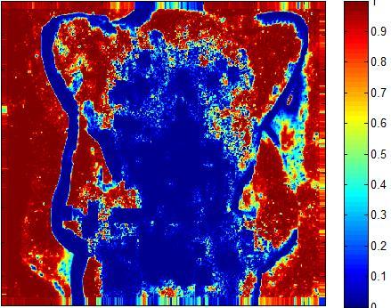
67 (a) (b) (c) (d) (e) (f) (g) (h) (i) (j) Figure 4.6: Visual Comparison of Blur Maps for the Proposed SVBD Algorithm and Existing methods. For Maps Shown in (c)-(j), Blue Values Correspond to Sharp (Low Blur Detection) Regions, and Red Values Correspond to Blurred (High Blur Detection) Regions. (a) Input; (b) Ground-Truth Mask (Black is Sharp and White is NonSharp); (c) Chakrabarti et al. [23]; (d) Su et al. [29]; (e) Zhuo et al. [85]; (f) Shi et al [28]; (g) Shi et al with Propagation [33]; (h) Shi et al without Propagation [33]; (i) Proposed SVBD Algorithm; (j) Proposed SVBD Algorithm with Matting. 55

68 recall into consideration, is used and is given by [99]: F = 2 precision recall precision + recall (4.19) Table 4.1 (second column) shows the resulting F-measure for the proposed SVBD and existing methods. From Table 4.1, it can be clearly seen that the proposed SVBD method results in the best F-measure, and thus achieves the best precision-recall performance as compared to the other six state-of-the-art methods. The result of the proposed SVBD algorithm could be further improved by including a post-processing matting operation [85], as shown in Fig. 4.5 and Table 4.1. For visual comparison, the resulting blur maps are also shown in Fig The results of Fig. 4.6 vividly demonstrate that the proposed SVBD method is able to obtain a consistently better blur detection result than existing competitive methods, while existing methods failed in some of the test cases. Finally, the computational cost of the proposed SVBD method is relatively low. The best existing method Shi et al. without propagation [33] is a l 1 -norm minimization problem, which is iterative and computational complex. Although Shi et al. without propagation [33] utilized the OMP-Box package [100] for a fast l 1 -norm minimization, however, it still takes a total of PL 2 + Q(2PL + K 2 L + 3KL + K 3 ) operations [100], where P is the size of the atom for the sparse dictionary, L is the number of the atoms in the dictionary, Q is the number of elements in the signal and K is the target sparsity. In the implementation of [33], P = 64, L = 128, Q is the number of the pixels in the test image and K = 64. So the method of [33] takes an average of operations per pixel in the test image. In the proposed SVBD algorithm, the Sobel edge detector takes 19Q operations; the edge gradient direction takes 6Q operations; the directional edge width computation takes 89Q operations for the worst scenario corresponding to the largest possible search range for local luminance extrema; the block contrast computation takes 3Q operations; the JNB computation takes Q operations; the probability of blur detection takes 5Q operations; the 56

69 local probability summation takes 258Q operations. So the proposed SVBD algorithm takes a total of only 381 operations per pixel in the test image, which is significantly lower than that of Shi et al. without propagation [33]. In addition, Shi et al. without propagation [33] requires offline training Blur Detection Evaluation on Perceptually Significant Pixels As we discussed in Section 4.4, perceptually less significant pixels have a relatively lower local variance and/or higher JND. Those pixels correspond to perceptually flat or near flat areas and play a less important role in blur perception, in contrast to perceptually significant pixels which have a relatively higher local variance and/or lower JND. To further validate the effectiveness of the proposed PS-SVBD algorithm, we provide the precisionrecall comparison by taking only those perceptually significant pixels into the evaluation of precision and recall. These perceptually significant pixels can be detected through the perceptual significance detection model as described in Section Here we use S RM > 1 to detect perceptually significant pixels in our implementation. The quantitative comparison results are shown in Fig Table 4.1 (third column) shows the resulting F-measure for the proposed PS-SVBD method and existing methods, when only perceptually significant pixels are taken into consideration. From Table 4.1, it can be clearly seen that the proposed PS-SVBD method results in the best F-measure, and thus achieves the best precision-recall performance as compared to the other six state-of-the-art methods. Similarily, the result of the proposed PS-SVBD algorithm could be further improved by including a post-processing matting operation [85], as shown in Fig. 4.7 and Table 4.1. Fig. 4.8 shows the resulting blur maps for several images using our proposed PS-SVBD scheme (Figs. 4.8(g) & (h)) and existing methods. For the blur maps shown in Figs. 4.8(b)- (h), blue values correspond to sharp (low blur detection) regions and red values correspond to blurred (high blur detection) regions. In addition, in the blur maps generated by the 57

70 Figure 4.7: Quantitative Comparison: Precision-Recall Curves for the Proposed and Existing Methods, Using Only Perceptually Significant Pixels for Evaluation. proposed PS-SVBD method (Figs. 4.8(g) & (h)), white values correspond to flat/near flat areas. None of the existing methods are able to detect these regions. Fig. 4.8 clearly shows that our proposed SVBD and PS-SVBD methods can better predict the perceived blur, while Shi et al [28] fails for the second test image and and Zhuo et al. [85] fails for the third test image. In addition, our proposed methods are not only capable to detect blur, but also to indicate the different amount of perceived blur. As shown for the third test image in Fig. 4.8, our method not only distinguishes two sharp and two blurred objects, but also assigns different values of perceived blur to those two relatively sharp objects, while the method in [28] fails to distinguish that the level of sharpness is different for these objects. Moreover, as shown in Figs. 4.8(g) & (h), our proposed PS-SVBD method is capable to detect and characterize flat/near flat regions in addition to sharp and blurred ones. 58

71 (a) (b) (c) (d) (e) (f) (g) (h) Figure 4.8: Visual Comparison of Blur Maps for the Proposed PS-SVBD Algorithm and Existing Methods. For Maps Shown in (b)-(h), Blue Values Correspond to Sharp (Low Blur Detection) Regions; White Values Correspond to Flat Regions; and Yellow to Red Correspond to Blur to More Heavily Blurred Regions. (a) Input; (b) Zhuo et al. [85]; (c) Shi et al [28]; (d) Shi et al with Propagation [33]; (e) Shi et al without Propagation [33]; (f) Proposed SVBD Algorithm with Matting; (g) Proposed PS-SVBD Algorithm; (h) Proposed PS-SVBD Algorithm with Matting. 4.6 Conclusion This chapter presents a perceptual-based Spatially Varying Blur Detection (SVBD) algorithm that is capable of generating a spatially varying blur map including the relative amount of local perceived blurriness. The proposed blur detection method involves direc59

72 tional edge spread calculation, probability of blur detection, and local probability summation. In addition, a local perceptual significance model is derived and incorporated into the blur detection resulting in a Perceptually Significant Spatially Varying Blur Detection (PS-SVBD) algorithm. This latter method enables the detection of perceivable blur while eliminating flat and near flat regions from the blur map. Experimental results and comparison with state-of-the-art blur detection methods show that the proposed methods outperform existing state-of-the-art blur detection methods both visually and quantitatively in terms of precision-recall. 60

73 Chapter 5 SELECTIVE PERCEPTUAL BASED IMAGE DEBLURRING In this chapter, we study the problem of image blind deblurring. State-of-the-art blind deconvolution methods are presented. After that, two selective perceptual-based image deblurring frameworks are demonstrated. The experimental results show that the proposed frameworks are capable of achieving a good reconstructed image quality for spatiallyvarying blurred images. 5.1 Introduction Image blur is caused by factors such as object-camera motion, defocus, atmospheric turbulence, and sensor limitations. Image deblurring is performed to recover a sharp version of a blurred input image. It is a long-standing challenging problem in the field of image processing, computational photography and computer vision. On one hand, image deblurring is useful to recover a high visual-quality image, which is of great importance in the field of consumer electronics, medical imaging and surveillance applications. On the other hand, image deblurring can be used to overcome camera limitations, in order to make imaging devices more affordable, compact and portable. In a typical image deblurring framework, a blurry image y is modeled as a convolution between a sharp image x and a blur kernel k, with additive noise n as follows: y = k x + n (5.1) Image deblurring methods can be categorized into non-blind image deblurring and blind image deblurring. In non-blind image deblurring/deconvolution, the blur kernel k is either given or can be estimated through a special calibration pattern in a controlled lab setup. Only x is unknown. Existing research on non-blind image deconvolution include the Richardson-Lucy method [101], and methods proposed by Krishnan and Fergus [102], Zoran and Weiss [103] and Joshi et al. [16], to name a few. For blind image deblurring, 61

74 both the blur kernel and desired sharp image are unknown. We will focus on blind deconvolution in this research. The blind deconvolution can be analyzed through a Bayesian framework by maximizing a posteriori probability (MAP), seeking a pair (x, k) maximizing [19]: p(x,k y) p(y,x k)p(x)p(y) (5.2) where is the proportional symbol. The blind deconvolution could also be performed by solving the following regularized cost minimization [104]: min x,k k x y λj(x) + γg(k) (5.3) where J(x) is the regularization term for x, G(k) is the regularization term for k, λ and γ are the weights for J(x) and G(k), respectively. When updating x and k simultaneously, the solution is referred to as a MAP x,k solution. Prior knowledge about the statistical distribution of natural images such as their sparse derivative distribution [105] is typically utilized as a regularization term when solving the blind deconvolution problem. Such prior knowledge is introduced in the hope of favoring natural images over unnatural ones as the desired solution. Different prior information is adopted for image deblurring, such as the l 2 -norm or l 1 -norm [105]. In addition, extra components are added to improve deblurring quality, including selecting sharp gradients/edges from the image [20, 21], and marginalization over all possible images [ ], in which the kernel estimation accounts for the covariance around x and not only for the mean solution. However, many of the existing image deblurring methods [19, 22, 34, 35] assume that the blur kernel is fixed for the entire image. In real-life applications, the defocus blur often varies spatially in an image, due to the fact that objects could be at different depths away from the lens. Blind deconvolution for spatially-varying blurred images is a more challenging task, as compared to non-blind deconvolution or non-varying blur cases. Many of the existing blind deblurring methods are either computationally costly and/or cannot perform reliably when dealing with spatially-varying blurred images, especially when the 62

75 blur is not caused by camera motion. These methods could potentially be applied to local image patches; still they generally do not take human perception into account. Certain regions of the image may not contain perceivable blur, thus no deconvolution is needed there. The application of the spatially-varying blur detection methods that were proposed in Chapter 4 can benefit the image blind deconvolution process by applying selectively the restoration to only those regions with perceivable blur, which may result in a reduction of restoration artifacts and a possible reduction in computational cost. Some existing methods claim to be applicable to performing a blind deconvolution for spatially-varying blurred images. But these methods either deal with motion blur [23] or require enough edges at most orientations [16]. These constraints greatly limit their reliability and possible applications to out-of-focus image deblurring. In addition, these existing methods do not take human perception into account. The remainder of this chapter is organized as follows. Firstly existing state-of-the-art blind deconvolution methods are presented. Then two selective perceptual-based image deblurring frameworks are presented, followed by experimental results. 5.2 Existing Blind Deconvolution Methods Hereby we discuss state-of-the-art blind deconvolution methods. A wide range of parametric image priors were proposed for image deblurring. The simplest choice is to use the l 2 -norm [19] penalties on the output of local derivative operators. However, one can easily find that the derivative histogram of a natural image is non-gaussian [19]. The l 2 -norm is not able to adequately model the sparse nature of common image and blur gradients, and results in deblurred images that are either over-smoothed or have ringing. Instead, many approaches use a l p -norm on the gradient, with p < 1 [105, 109, 110]. This exponential distribution with p smaller than one is sparse, encourages small values and punishes large values in the image gradient distribution, reflecting the statistics of natural images. Another alternative for regularization is the use of total variation (TV) [111]. For a real-valued 63

76 continuous function, its total variation is a measure of the one-dimensional arclength of the curve on the interval of definition [112]. However, total variation may introduce loss of contrast in the reconstructed image [113]. Levin et al. [19] show that the direct application of many commonly used sparse derivative prior in a MAP x,k framework fails to reach the desired sharp image solution. To be more specific, the MAP x,k score does favor sharp signals for step edges, and thus steering it towards the sharp solution. However, it is not the case for impulse edges and sharp natural images [19]. So many of those MAP x,k algorithms require additional components to reach the desired sharp image solution. Some methods use heuristics to select sharp gradients/edges [20, 21], in order to reduce the generation of artifacts. Others include spatially-varying prior terms [114], computing marginal probabilities over all possible images [19, ] and determining of the edge locations using shock filtering [115]. Levin et al. [19] propose the MAP k estimation while marginalizing over x. This is proposed based on the fact that the dimensionality of k is relatively small. While a simultaneous MAP x,k estimation fails to reach the desired sharp image solution, a MAP k estimation of k alone (marginalizing over x), is well constrained and recovers an accurate kernel [19]. Such MAP k estimation can be expressed as follows: ˆk = arg max p(k y) = arg max p(x,k y)dx (5.4) The computation of MAP k is challenging since it involves a computationally intractable marginalization over all possible x explanations. Approximation methods of MAP k are adopted, such as the EM MAP k approach of Levin et al. [34]. In more recent developments of blind deconvolution, Babacan et al. [35] presented a general method for blind image deconvolution using Bayesian inference with super- Gaussian sparse image priors. Sun et al. [116] explored a new approach for kernel estimation from a single image via modeling image edge primitives using patch priors. Both a statistical prior learned from natural images and a simple synthetic prior are examined. 64

77 Xu et al. [117] proposed a new sparse l 0 approximation scheme. Perrone et al. proposed projected alternating minimization in [113] and developed a blind deconvolution method based on a family of logarithmic image priors [118]. Krishnan et al. [22] proposed to use the ratio of l 1 -norm to l 2 -norm for image regularization in a MAP x,k approach, which favors sharp images over blurry ones. The l 1 -norm is generally used to impose signal sparsity and penalize the high frequency bands. When an image is more blurred, its high frequency components get reduced as well as their l 1 -norm. Minimizing the l 1 -norm will favor blurry images and a delta kernel, instead of a sharp image and a blur kernel. The l 1 /l 2 ratio is a normalized version of the l 1 -norm. When the image is more blurred, both the l 1 -norm and the l 2 -norm decrease but the l 2 -norm decreases faster. This regularizer compensates for the attenuation of high frequencies and therefore favors a sharp image and a blur kernel. The cost function is modeled as: min x,k k x y x 1 x 2 + ψ k 1 (5.5) Similarly like other MAP x,k algorithms, this method [22] alternates between two main steps: 1) set k constant and solve for the best x, and 2) set x constant and solve for the best k. The x sub-problem is non-convex due to the l 1 /l 2 term. The iterative shrinkagethresholding algorithm (ISTA) [119] is adopted by fixing the denominator of the regularizer from the previous iteration and solving the convex l 1 -norm regularized problem. Unconstrained iterative re-weighted least squares (IRLS) is used for the k sub-problem [22]. 5.3 Proposed Selective Perceptual-Based Image Deblurring-I (SPID-I) Framework Fig. 5.1 shows a block diagram of the proposed selective perceptual-based image deblurring- I (SPID-I) framework. The application of the proposed selective perceptual significant blur detection framework (Chapter 4) will benefit the image blind deconvolution process by applying the restoration process selectively to a small set of perceptually significant blur locations, thus significantly reducing the restoration artifacts. As shown in Fig. 5.1, a perceptually significant blur map is first generated for the considered input image using 65

78 Figure 5.1: Diagram of The Proposed Selective Perceptual-Based Image Deblurring-I (SPID-I) Framework. the proposed PS-SVBD method. The generated blur map has a high value at perceptually significant blur pixels, as discussed in Chapter 4. Then a selected image patch is deblurred only when the patch contains perceptually significant blur pixels. The deconvolution kernel is estimated by applying the selected blind deconvolution method to the considered image patch. Then the estimated kernel is applied through a non-blind devolution operation on the same patch, to get the initial deblurred result of the considered patch. The binarized blur map is applied to merge the initial deblurred result and the input image. Only those perceptually significant blur pixels will be updated using the pixel value of the initial deblurred result. 5.4 Experimental Results for the SPID-I Framework Here we use a test image with a spatially varying blur to demonstrate the proposed SPID-I framework, as shown in Fig Four different patches are chosen at different distances 66

79 Figure 5.2: The Test Image to Demonstrate the Proposed SPID-I Framework. from the camera. In addition to the proposed SPID-I method, three state-of-the-art methods are compared including Babacan et al. [35], Levin et al. [34], and Krishnan et al. [22]. The obtained performance results and comparisons with existing methods using different patches are presented in Fig. 5.3 to Fig It can be clearly seen that the proposed SPID-I method results in the best visual quality for the deblurred image. In comparison, the results of Babacan et al. [35] and Levin et al. [34] methods are less sharp. The Krishnan et al. [22] is capable of getting the sharpest reconstructed results among those three existing methods, while it suffers from reconstruction artifacts in the non-blur region. In the proposed SPID-I framework, the final deconvolution result is generated by merging the input image with the deblurred result of the method of Krishnan et al. [22], based on the binarized blur map, by only updating the perceptually significant blurred pixels of the input image (bina- 67

80 (a) (b) (c) (d) (e) Figure 5.3: Comparison of Image Deblurring, test patch 1. (a) Original Input Image. (b) Babacan et al. [35]. (c) Levin et al. [34]. (d) Krishnan et al. [22]. (e) Proposed SPID-I Method. 68

81 (a) (b) (c) (d) (e) Figure 5.4: Comparison of Image Deblurring, test patch 2. (a) Original Input Image. (b) Babacan et al. [35]. (c) Levin et al. [34]. (d) Krishnan et al. [22]. (e) Proposed SPID-I Method. rized blur map is 1 at these pixels locations) with their corresponding deblurred values. The deblurring results of the proposed SPID-I framework preserve the sharpness of the method of Krishnan et al. [22], while significantly reducing the restoration artifacts. 5.5 Proposed Selective Perceptual-Based Image Deblurring-II (SPID-II) Framework In the proposed SPID-I framework, for different patches within the same image, the deconvolution kernel need to be estimated again. Since the kernel estimation is computational much more expensive than non-blind devolution, it would be beneficial if the estimated kernel could be applied to other patches with a similar blur level. The proposed SVBD algorithm is capable of generating a blur map indicating the relative amount of perceived local blurriness. The generated blur map could be used as a guidance to selectively apply 69

82 (a) (b) (c) (d) (e) Figure 5.5: Comparison of Image Deblurring, test patch 3. (a) Original Input Image. (b) Babacan et al. [35]. (c) Levin et al. [34]. (d) Krishnan et al. [22]. (e) Proposed SPID-I Method. the estimated kernel to other blur patches. Many natural images are composed of background and foreground. While the blur level for the background and foreground are quite different, the blur level within the background or the foreground could be relatively close. The proposed SPID-II framework is especially useful for these cases. As illustrated in Fig. 5.7, the blur map is generated using the proposed SVBD algorithm, and a local patch is selected in the blur region. Then the deconvolution kernel is estimated by applying a blind deconvolution on the considered local patch. The estimated kernel is then applied to other local patches whose blur level is close to the local patch that was used to estimate the blur kernel. 70

83 (a) (b) (c) (d) (e) Figure 5.6: Comparison of Image Deblurring, test patch 4. (a) Original Input Image. (b) Babacan et al. [35]. (c) Levin et al. [34]. (d) Krishnan et al. [22]. (e) Proposed SPID-I Method. 5.6 Experimental Results for the SPID-II Framework Here we use three natural images to demonstrate the proposed SPID-II framework. The results are shown in Fig As described in the SPID-II framework, a deconvolution kernel is estimated by applying a blind deconvolution to the considered image local patch. In this experiment, the applied kernel estimation method is Krishnan et al. [22] and the image local patch is chosen as a rectangular region in the background. If the same deconvolution kernel is applied to the whole image through non-blind deconvolution, the deblurring result is shown in Fig. 5.8(d). The applied non-blind deconvolution is Krishnan et al. [102]. While the originally blurry background does get sharper, this method creates a lot of restoration artifacts in the foreground. Our proposed SPID-II framework is capable of differentiating the blur region and sharp region, and applying the deconvolution 71

84 Figure 5.7: Diagram of the Proposed Selective Perceptual-Based Image Deblurring-II (SPID-II) Framework. selectively to the blur region, which significantly reduces the restoration artifacts, while preserving the sharpness of the deblurred image. The corresponding objective comparisons are provided in Table. 5.1 using the CPBD [5] and SSIM [47] objective quality assessment methods. SSIM [47] is used to evaluate the fidelity between the sharp region of the input image and the same region of the deblurred results. CPBD [5] is used to evaluate the sharpness of the blur region. As shown in Table. 5.1, when the same deconvolution kernel is applied to the whole image, the resulting deblurred image has a higher CPBD than the original image, indicating an increase in image sharpness; however, the resulting deblurred image leads to a reduced SSIM for the sharp regions due to the introduction of restoration artifacts. The proposed SPID-II framework results in a high CPBD for the deblurred blur regions, while maintaining a high SSIM 72

85 (a) (b) (c) (d) (e) Figure 5.8: Visual Results for the Proposed SPID-II Framework. For Maps Shown in (c), Red Values Correspond to Blurred (High Blur Detection) Regions, and Blue Values Correspond to Sharp Regions. (a) Input Image; (b) Grayscale Input Image; (c) Blur Map Generated by the SVBD Algorithm with Matting; (d) Deblurring Result when Applying One Estimated Kernel globally; the Kernel is Estimated Using a Blurred Patch; (e) Deblurring Result of the Proposed SPID-II Framework; One Kernel was Estimated. Table 5.1: Objective Quality Comparison of the Input Image and Deblurred Results. CPBD on blur region SSIM on sharp region Input image Results of Fig. 5.8(d) Proposed SPID-II Input image Results of Fig. 5.8(d) Proposed SPID-II bald women owl for the sharp regions. For the results in Fig. 5.8, we only consider the image to consist of two types of regions: sharp regions and blur regions (two blur levels). We then apply the same deconvolution kernel throughout to the blur region. A more general setting of the SPID-II framework is shown in Fig It could consider multiple quantized blur levels in the blur region by quantizing the blur map that is generated by the SVBD/PS-SVBD algorithms. In addition, 73

86 Figure 5.9: Diagram of the Proposed Selective Perceptual-Based Image Deblurring-II (SPID-II) Framework, a More General Setting. the sharp region could be considered as a region with low levels of blur. In the following, the entire image is categorized into three regions, based on the blur map. One deconvolution kernel is estimated per blur level, and selectively applied to the subregion of the corresponding blur level only. The results are shown in Fig The corresponding objective comparisons are provided in Table. 5.2 using CPBD [5]. The obtained results show that the proposed SPID-II framework could achieve sharp restoration results, and can be applied to more complex images with multiple blur levels. 74

87 (a) (b) (c) (d) Figure 5.10: Visual Results for the Proposed SPID-II Framework in a More General Setting. For Maps Shown in (c), Red Values Correspond to Blurred (High Blur Detection) Regions, and Blue Values Correspond to Sharp Regions. (a) Input Image; (b) Grayscale Input Image; (c) Blur Map Generated by the SVBD Algorithm with Matting; (d) Deblurring Result Using the Proposed SPID-II Framework, Three Kernels were Estimated. Table 5.2: CPBD [5] Comparison of the Input Image and Deblurred Results. Input image Proposed SPID-II region region region overall region region region overall soldier hat bird

88 Chapter 6 EDGE ENHANCED SUPER RESOLUTION Edge regions play an important role in the quality of the super-resolution (SR) results. In the existing adaptive Wiener filter based SR algorithm [36], a universal auto-correlation model is used for both the edge regions and other regions. This leads to a not-as-sharp reconstruction of the edge regions. In the proposed Edge-Enhanced SR (EE-SR) algorithm, distributed edge detection is used to detect the edge regions. Then a refined estimation of the edge regions is conducted based on the auto-correlation characteristics of the edge regions. Experimental results show that the proposed EE-SR algorithm achieves a better reconstruction quality than existing algorithm of [36]. In the proposed EE-SR method, only the edge regions get updated so that limited calculations are added. 6.1 Introduction Super-resolution (SR) is widely used to increase the image resolution by fusing several low resolution (LR) images in the same scene to overcome sensor limitations and image impairments in a cost-effective manner [120]. Image impairments such as sensor noise, packet loss and compression, can be reduced through SR. In addition, advances in display technologies and the increase of hardware computational capabilities enabled the development of efficient and effective super-resolution techniques. SR algorithms can be divided into several categories. Maximum A Posteriori (MAP) based [36] regularized norm-minimization solutions can converge to a high quality result but are iterative and exhibit a relatively high computational complexity. MAP-based SR methods have the advantage of being able to include prior knowledge into the observation model. However, these methods are sensitive to the assumed statistical models for the data and noise. To reduce the computational complexity and enhance the robustness to noise, a Fusion-Restoration method [37] was proposed using l 1 -norm minimization and a robust regularization based on a bilateral prior. However, this method is still iterative and com- 76

89 putationally intensive due to the high dimensionality of the problem. Karam et al. [38] exploit human perception resulting in significant reduction in computations for iterative SR approaches and an improved SR visual quality. Another faster non-iterative Fusion- Interpolation (FI)-based SR approach [3] requires less computation but suffers from a limited reconstruction quality. It is found that the SR result of the FI-based SR approach [3] does not result in a satisfactory reconstruction of the strong edges in the image, and results in a significantly blurred reconstruction of weak edges. To tackle this issue, this chapter proposes an Edge-Enhanced SR (EE-SR) approach, in order to achieve a higher reconstruction quality without significantly increasing the computational complexity. Experiments show that the proposed FI-based EE-SR algorithm results in sharper edges as compared to the existing FI-based SR approach. The remainder of this chapter is organized as follows. Section 6.2 describes the observation model. Section 6.3 describes the proposed EE-SR approach. Experimental results are given in Section 6.4, followed by subjective quality assessment results in Section 6.5 and a conclusion in Section Observation Model The observation model assumes that all LR images are generated from the same HR image, with different sub-pixel shifts between LR frames. Due to the fractional pixel LR shifts, registered HR samples will not always fall on a uniformly spaced HR grid, thus providing over-sampled information necessary for solving the SR inverse problem. After the geometric transformation, the LR pixels are defined as a weighted sum of appropriate HR pixels. The weighing function models the blurring caused by the system point spread function (PSF). After that, an additive Gaussian noise is added to represent random errors and sensor noise. Since the LR images are acquired from the same HR image, and using the same camera with the same resolution enhancement ratio, it is reasonable to assume that the PSF and the noise are static for all LR observations. Now we can express the kth 77

90 LR frame as : Y k = DHF k Z + n (6.1) where Z represents the lexicographically ordered HR image, n is the additive noise modeled as an independent and identically distributed (i.i.d.) Gaussian random variable with variance σ 2 n, F k is the warping matrix, H is the blurring matrix representing the common PSF function, and D is the decimation matrix. 6.3 Proposed Edge Enhanced SR (EE-SR) Approach An edge-enhanced SR (EE-SR) approach is proposed to achieve a better reconstruction quality for the edge regions. It can be divided into three steps: initial SR estimation, distributed detection of edge regions and the refined SR estimation of edge regions pixels. In our implementation, the initial SR estimation is based on the adaptive Wiener filter super-resolution (AWF-SR) method [3] Initial SR Estimation Fused LR samples are processed locally using a moving observation window to estimate the interpolation kernel and an estimation window to apply the designed kernel on the spanned LR observed samples in order to estimate the missing HR pixels. Let i be the index of the considered observation window, L be the SR ratio, and N be the number of LR frames. Also Assume the size of the observation window is M 2 pixels on the high resolution grid and that it spans a total of K = (N M 2 )/L 2 LR pixels represented by the observation vector G i of length K. The estimation window is a subwindow within the observation window and is composed of D x D y pixels on the high resolution grid. As proposed by Hardie et al. [3], estimating the HR vector D i in the local estimation window is achieved by applying locally designed kernel weights W i to the observation vector G i, as follows: D i = W T i G i (6.2) 78

91 where W i is a K D x D y matrix of weights given by W i = R 1 i P i (6.3) where R i is the autocorrelation matrix of the observation vector, and P i is the crosscorrelation between the desired vector D i and the observation vector G i. Define F i as the noise-free version of the observation vector G i and n i as the zero-mean Gaussian noise with standard deviation of σ n. G i, R i, and P i can then be expressed as: G i = F i + n i (6.4) R i = E(G i G T i ) = E(F i F T i ) + σ 2 n I (6.5) P i = E(G i D T i ) = E(F i D T i ) (6.6) The continuous-domain cross-correlation function R DF (x,y) and autocorrelation function R FF (x,y) can be written as follows: R FF = R DD (x,y) h(x,y) h( x, y) (6.7) R DF = R DD (x,y) h(x,y) (6.8) In the above expressions, R DD (x,y) is defined as a continuous domain wide sense stationary auto-correlation function for the desired HR coefficients D i, h(x,y) is the continuous domain blurring function, and x and y are continuous spatial distances between pixels. The horizontal and vertical distances between observation pixels can be easily computed. Evaluating (6.7) using all these displacement yields E(F i F T i ), then R i can be calculated using (6.5). Similarly, P i can be calculated using (6.8) and (6.6). Now the problem of computing the filter weights reduces to modeling the auto-correlation function R DD. In [3], the auto-correlation function is modeled using a spatially varying circularly symmetric parametric auto-correlation model as follows: R DDi (x,y) = σ 2 D i ρ x 2 +y 2 (6.9) 79

92 where ρ is a tuning parameter and σ Di is the standard deviation of the local region of the desired image D i and can be expressed as: in (6.10), C(ρ) can be expressed as: C(ρ) = σ 2 D i = 1 C(ρ) σ 2 F i = 1 C(ρ) (σ 2 G i σ 2 n ) (6.10) ρ x 2 +y 2 h(x,y) h( x, y)dxdy (6.11) and σ Gi is the standard deviation of the elements of the observation vector G i. The above expressions (6.10) and (6.11) suggest that ρ in (6.9) can be approximated using the linear mapping between σ Di and σ Fi during the training process. ρ = 0.75 is used in Hardie et al. [3]. It is worth indicating that both the peak value σ 2 D i and the decay of the spatially varying auto-correlation model in (6.9) are affected by ρ. Equation (6.9) is the key model to generate a proper weight matrix and to reconstruct the HR image. Although R DD adapts to the variance of the HR coefficients in each local observation window, still, this global assumption of the same ρ leads to an improper modeling of the autocorrelation function, especially for edge regions. The reconstruction quality of edge regions greatly affects the visual quality of the SR result due to the perceptual significance of these regions. The autocorrelation model of these edge regions differs from those of non-edge regions. In order to better model the autocorrelation of edge regions, edge detection is performed using a distributed Canny edge detector [39] that is applied to the initial SR estimated results Distributed Detection of Edge Regions The Canny edge detector is commonly used to detect edge pixels. The Canny edge detector consists of gradient calculation, non-maximal expression, thresholds computation and hysteresis thresholding. The high and low thresholds are computed using the gradient magnitude cumulative distribution function (CDF) of the entire image. The utilization of 80

93 (a) (b) (c) (d) Figure 6.1: Comparison of the Traditional Canny and Distributed Canny Edge Detectors. (a) Original Image. (b) Initial SR Result using AWF-SR [3]. (c) Traditional Canny Edge Detection Result. (d) Distributed Canny Edge Detection Result. Figure 6.2: Test images for Super-Resolution. the entire image statistics bring the advantage of good edge detection, but also is not practical for large image sizes and does not support parallel processing. One simple solution is to use the image statistics of local image windows instead of the entire image. However, directly applying the original Canny at a local window level would fail since it leads to excessive edges in the smooth region and loss of edges in the sharp region. A distributed Canny edge detector was proposed in [39], by simultaneously computing thresholds for each block, based on the block type and the local distribution of gradients. The image blocks are classified as smooth, texture, hybrid and strong edge, based on the block clas- 81

94 sification method of Su et al. [121]. Also, for each block type, the appropriate percentage values which correspond to the high threshold and low threshold are selected differently. Applying the distributed Canny edge detector brings several advantages to proposed EE-SR algorithm: 1) The distributed Canny detector better adapts to the local image characteristics than the original Canny edge detector; so some weak edges can be detected, as shown in Fig. 6.1; 2) for the sake of computational cost, the proposed algorithm can be applied only to selected region of interest. When using the distributed Canny edge detector, the proposed EE-SR algorithm can be applied in a locally adaptively manner Refined Estimate of Pixels in Edge Regions The tuning parameter ρ plays an important role in the autocorrelation model of (6.9). It is not ideal to use one single universal ρ for both edge regions and flat regions, even after taking the variance of the local window into consideration. A higher ρ models a relatively flat auto-correlation in the reconstructed SR image. It is adequate in flat regions and removes most of the noise. However, it leads to a not-as-sharp reconstruction for the edges. A lower ρ models a relatively sharp auto-correlation in the reconstructed SR image. It suits edge regions well for a sharper reconstruction. However, it leads to a noisy result for the flat regions. In [3], ρ = 0.75 is used no matter whether the considered region is an edge region or a flat region. Although the variance of the local window is taken into consideration, such fixed single value fails to produce a high reconstruction quality for the edge regions. Here we keep the symmetric autocorrelation model of (6.9) but adapt the ρ value based on the characteristics (edge or flat) of the considered region. We define ρ e as the ρ for the edge regions. In this work, ρ e is set to 0.45 and is used to model the autocorrelation function for edge regions. 6.4 Experimental Results In this section, the performance of the proposed EE-SR algorithm is assessed using a set of test images as shown in Fig A sequence of LR images is generated from a single 82

95 (a) (b) (c) (d) Figure 6.3: Comparison of SR Results. (a) Original HR Image. (b) SR Result Using Single Frame Bi-cubic Interpolation. (c) SR Result Using AWF-SR [3]. (d) SR Result of the Proposed EE-SR Algorithm. HR image. For example, the original HR image is used to generate 16 LR images of The original HR image is shifted according to given motion vectors at various directions and values. Then the shifted images are blurred by an averaging 4 4 filter to model sensor integrations and are down-sampled by 4 in both directions. Additive Gaussian noise is then added to represent random errors and sensor noise. Two different noise variances are used, including σn 2 = 100 and σn 2 = 30. As shown in Fig. 6.3, the edge region of our proposed EE-SR algorithm is slightly sharper and more detailed through edge region refined estimation. Tables 6.1 and 6.2 present the performance of the proposed EE-SR algorithm for σn 2 = 30 and 100, respectively, in addition to comparison with existing methods using multiple quality metrics. From Tables 6.1 and 6.2, it can be clearly seen that the proposed algorithm results in the 83

96 Table 6.1: Objective Quality Comparison of SR Results (Noise Variance = 30). PSNR SSIM CPBD Bi- AWF EE- Bi- AWF EE- Bi- AWF EEcubic [3] SR cubic [3] SR cubic [3] SR ISOchart a ISOchart b aerialcrop buildings cameraman character clock reso chart sandiego text Table 6.2: Objective Quality Comparison of SR Results (Noise Variance = 100). PSNR SSIM CPBD Bi- AWF EE- Bi- AWF EE- Bi- AWF EEcubic [3] SR cubic [3] SR cubic [3] SR ISOchart a ISOchart b aerialcrop buildings cameraman character clock reso chart sandiego text best performance in terms of all the metrics including PSNR and the more perceptually motivated ones such as SSIM [47] and CPBD [5]. The increase in SSIM shows that the SR result of the proposed algorithm achieves a better reconstruction quality. In addition, higher CPBD shows that the SR result of the proposed EE-SR algorithm achieves a sharper reconstructed results for edge regions. 84

97 Figure 6.4: Subjective Test Interface. 6.5 Subjective Quality Assessment A subjective experiment is conducted to compare the SR results of the proposed EE-SR algorithm and AWF-SR [3]. In the subjective quality assessment, seventeen human subjects are asked to compare the sharpness and overall quality between the proposed EE-SR algorithm and AWF-SR [3]. The subjective test interface is shown in Fig 6.4. The scores given by observers are averaged to produce the Mean Opinion Score (MOS), including MOS-sharpness and MOS-overall. Source Image Content: Ten gray source images are used, and included natural images, remote sensing images and OCR images. Two different noise variances are used including σn 2 = 100 and σn 2 = 30. These test images and noise variance are the same as those mentioned in Table 6.1 and Table 6.2. A total of different 20 image pairs are used in the experiment. Each pair includes the result of the proposed EE-SR algorithm and the corre- 85

98 sponding result of AWF-SR [3], with randomized order. Each image pair is repeated four times. Equipment and Display Configuration: The experiment was conducted using a inch LCD monitor (DELL Alienware 2310) with a 120 Hz refresh rate, at a distance of 24 inches. The room illumination was 500 lux. Subjects: Seventeen subjects participated in the subjective testing. All subjects were screened for visual acuity (20/20). Test Methodology: We used a pair-wise methodology. Each pair includes the result of the proposed EE-SR algorithm and the corresponding result of AWF-SR [3], with randomized order. Subjects were asked to judge their preference on image sharpness and image overall quality, for each image pair, respectively. Subjects were asked to score the quality using a five-grade scale (Left Better, Left Slightly Better, Same, Right Slightly Better, Right Better). Each subject was individually briefed about the goal of the experiment, and given a demonstration of the interface and the procedure. The display order of the test images was randomized each time for each subject. Fig. 6.5 and Fig. 6.6 show the obtained MOS-sharpness and MOS-overall. The MOS ranges from 0 to 5. A MOS larger than 3 indicates that the subjects preferred the proposed EE-SR algorithm over AWF-SR [3], while a MOS smaller than 3 indicates otherwise. Fig. 6.5 shows that the proposed EE-SR algorithm always generates sharper SR results than AWF-SR [3]. This corresponds well with the CPBD [5] results in Table 6.1 and Table 6.2. Fig. 6.6 shows that when it comes to overall quality, subjects preferred the proposed EE-SR algorithm over AWF-SR [3] in three-quarters of the cases. The proposed EE-SR algorithm always generates sharper SR results, however, it might introduce slightly more reconstruction artifacts near edge regions as compared to AWF-SR [3], as shown in Fig This is because that the initial SR results generated by AWF-SR [3] typically have some ringing artifacts, which might be detected as edge in the edge detection. So for these regions, ρ e will be used as their local autocorrelation parameter. These lead 86

99 Figure 6.5: MOS Sharpness for the Subjective Experiment of the SR Results. A Score Value Greater than 3 Indicates That the Proposed EE-SR Algorithm Achieves in a Better Perceived Sharpness than the Existing AWF-SR Method [3]. to slightly more reconstruction artifacts in EE-SR, when compared with AWF-SR [3]. The reconstruction artifacts are more obvious in high noise cases, as it can be seen from Fig Conclusion This chapter presents an edge-enhanced SR (EE-SR) algorithm that adapts the autocorrelation model to local image characteristics including edge regions and flat regions. First the initial SR result is computed. After that, the SR result is refined in the edge regions using an autocorrelation model whose parameter is adjusted for the edge regions. Experimental results including image quality metrics and subjective scores are provided to demonstrate the effectiveness of the proposed EE-SR algorithm. 87

100 Figure 6.6: MOS Overall for the Subjective Experiment of the SR Results. A Score Value Greater than 3 Indicates That the Proposed EE-SR Algorithm Achieves a Better Perceived Visual Quality than the Existing AWF-SR Method [3]. (a) (b) (c) (d) Figure 6.7: Comparison of SR Results. (a) SR Result Using AWF-SR [3] (Noise Variance = 30). (b) SR Result of the Proposed EE-SR Algorithm [3] (Noise Variance = 30). (c) SR Result Using AWF-SR [3] (Noise Variance = 100). (d) SR Result of the Proposed EE-SR Algorithm [3] (Noise Variance = 100). 88