ANALYSIS AND DESIGN OF A TWO-WHEELED ROBOT WITH MULTIPLE USER INTERFACE INPUTS AND VISION FEEDBACK CONTROL ERIC STEPHEN OLSON

Transcription

1 ANALYSIS AND DESIGN OF A TWO-WHEELED ROBOT WITH MULTIPLE USER INTERFACE INPUTS AND VISION FEEDBACK CONTROL by ERIC STEPHEN OLSON Presented to the Faculty of the Graduate School of The University of Texas at Arlington in Partial Fulfillment of the Requirements for the Degree of MASTER OF SCIENCE IN MECHANICAL ENGINEERING THE UNIVERSITY OF TEXAS AT ARLINGTON August 2010

2 Copyright by Eric Stephen Olson 2010 All Rights Reserved

3 ACKNOWLEDGMENTS I would like to thank Dr. Panayiotis Shiakolas for being my advisor for this thesis and for all his guidance and encouragement. I would also like to thank Richard Margolin for lending me his expertise in choosing and debugging hardware. Finally, I would like to thank Dr. Alan Bowling, and Dr. Kamesh Subbarao for serving on my thesis committee. July 16, 2010 iii

4 ABSTRACT ANALYSIS AND DESIGN OF A TWO-WHEELED ROBOT WITH MULTIPLE USER INTERFACE INPUTS AND VISION FEEDBACK CONTROL Eric Stephen Olson, M.S. The University of Texas at Arlington, 2010 Supervising Professor: Panayiotis Shiakolas This thesis describes the development of a small, inexpensive, controllable mobile two-wheeled robot. It also describes the development of a software interface which allows several open- and closed-loop control methods to be easily implemented. The developed hardware and software modules provide for an open and modular system for research purposes. This is demonstrated through the Bluetooth wireless control of the robot using LabVIEW based software modules. The open-loop control inputs implemented are sliders in a LabVIEW GUI, joystick, and voice commands. The closed-loop control methods included a PD control algorithm that guides the robot to go directly to a user defined point, and a path planning control algorithm that guides the robot to follow a path and reach the user defined goal in the correct orientation. The closed-loop control methods use an external camera for vision based position feedback. All the control methods introduced were successfully tested experimentally. iv

5 TABLE OF CONTENTS ACKNOWLEDGMENTS... iii ABSTRACT..... iv TABLE OF CONTENTS... v LIST OF ILLUSTRATIONS... vii Chapter Page 1. INTRODUCTION ANALYSIS Dynamic Modeling and Simulation Kinematic Analysis Control Algorithm PD Control Control Method Control Method Path Planning EXPERIMENTAL PROCEDURE Mechanical Design Hardware/Computer Interface LabVIEW Motor Control Board & Bluetooth Module Characterizing the Device Open-Loop Control: LabVIEW GUI, Joystick, Voice v

6 3.5 Vision Feedback Control Calibration Defining the Desired Position Control Algorithm Path Planning CONCLUSIONS AND RECOMMENDATIONS FOR FUTURE WORK Discussion Future Work APPENDIX A. SOLVING POLYNOMIAL COEFFICIENTS B. ORIGINAL AUTOLEV MODEL OF A TWO-WHEELED ROBOT C. SIMPLIFIED AUTOLEV DYNAMIC MODEL D. CONTROLLER STABILITY E. PARTS UTILIZED F. WIRING DIAGRAM G. LABVIEW GUI H. EXAMPLE LABVIEW CODE I. SETUP REFERENCES BIOGRAPHICAL INFORMATION vi

7 LIST OF ILLUSTRATIONS Figure Page 1.1 Two-Dimensional Rolling Robot Two-Dimensional Rolling Robot Model Two-Dimensional Simulation Example (Modified PD Control) CAD and Simulated Models of Shell Rolling Robot Shell Rolling Robot Example Simulation Generalized Coordinates of the Two-Wheeled Robot CAD Model of the Two-Wheeled Robot Two-Wheeled Robot Example Simulation Simplified Two-Wheel Robot Diagram Two-wheeled Mobile Robot Motion Variables Graphical Relationship between and, and,, and Graphical Relationship between and, and and Example Control Setup Showing Initial Error Example of Eliminating by Reorientation Examples of PD control Path Following Example Desired and actual and, and error over time Discontinuous Path Following Example vii

8 2.18 Path Generation Examples Autolev Dynamic Model Generalized Coordinates Fabricated and Assembled Robot CAD Model of the Robot Robot Drive System Robot Electronics Relations Between Components Motor Characterization Setup Device Characterization Result Modular Open-Loop Controls Camera Calibration Pixel Space to Real Space VI Pattern for Vision Matching Path Planning LabVIEW Code Examples of Paths Generated Size of Robot Without Electronics viii

9 CHAPTER 1 INTRODUCTION There are many discussions of rolling mobile robots in the literature. The advantage of these types of robots is the simplicity of their driving mechanisms, which makes them good candidates for miniaturization. The most common type of rolling robot is actuated by shifting the center of mass (CG) of the robot so that a moment is created about the point at which the robot is in contact with the ground, as is illustrated in figure 1.1. An example of a two-dimensional mechanism similar to the one shown in Figure 1.1 is discussed in [1]. Figure 1.1 Two-Dimensional Rolling Robot Although there are other types of rolling robots, for example the one discussed in [2] where a spherical robot is actuated by taking advantage of the conservation of momentum using flywheels. In [2] the research focuses on rolling robots that are 1

10 actuated by shifting the CG. There are two major categories of how to apply the principle shown in Figure 1.1 to robots in three dimensions. One category is shell robots. This type of robot is the most obvious extension of the two-dimensional robot shown in Figure 1.1. This type of robot consists of an outer shell (usually a sphere) and some mechanism inside the shell to move the CG of the shell off center. The second major category of rolling robots is the two-wheeled robot. This type of robot consists of two parallel wheels on one axis and a body that connects the two wheels. The two wheels can be thought of as two separate two-dimensional rolling mechanisms similar to Figure 1.1, and the body of the robot does not coincide with the axis of the robot and is used to create the off-centered CG. Within the category of shell robots there are three basic types. The first type has a spherical shell, and inside the shell there is a pendulum mass attached to a two-degreeof-freedom actuated gyroscope [3, 4]. This allows the center of mass of the robot to be offset in any direction which allows this type of robot to move in any direction without turning. This makes this type of robot very agile, however, because of the nature of the mechanism, this robot must have a large amount of empty space on its inside which makes it a poor candidate for miniaturization. The second type of shell robot also consists of a shell and a pendulum weight, however, the weight is only able to rotate fully about a primary axis, and to a limited degree about a secondary axis [5, 6]. This means that this type of robot has a definite orientation. It primarily moves forwards and backwards in a direction perpendicular to the primary axis, and the limited rotation about the secondary axis is used to turn the robot. The advantage of this robot is that it 2

11 is more compact than the first type of shell robot. However, it is more limited in its motion, and it has a relatively large minimum turning radius. The third type of shell robot consists of a spherical shell with masses inside that move back and forth along spokes [7, 8]. This type of rolling robot, like the first type, has the advantage of being able to move in any direction without reorientation. The disadvantage of this type of robot is that it requires at least three linear actuators, while the other two types require only two rotational actuators. The other major category of rolling robots is the two-wheeled robot. Twowheeled robots are the most prevalent rolling robots in the literature. The prevalence of these robots stems from a crucial advantage they present over other varieties of rolling robots in that they do not have a minimum turning radius. There are several different variations of two-wheeled robots. There are ones that have their CG above their wheel axis. An example of a mechanism like this is the Segway. These types of robots are inherently unstable and require a control system to remain upright and balanced [9]. There are also two-wheeled robots which have their center of mass below the axis of the wheels [10-12]. These types of robots are statically stable although they are subject to oscillations. Finally there are robots which have the kinematics of a two-wheeled robot, but are not true rolling robots. These robots have two main wheels which behave like other two wheeled robots, but they also have one or more idler wheels to keep them from rotating about their wheel axis [13, 14]. The advantage of these robots is that they are easier to control than the other two wheeled robot types because they do not have as many degrees of freedom, however, they require smoother operating environments. 3

12 The research presented in this thesis studied concepts previously described in the literature and then developed a small, inexpensive version of a rolling robot. The objectives included simulating, designing, fabricating, assembling, and interfacing the electrical components of the robot, and developing a modular and easily expandable software interface so that new hardware can be interfaced easily, and different path planning and control algorithms can be easily implemented and verified. This was accomplished by examining the different types of rolling robots in the literature to weigh their pros and cons. Then a few designs were selected, including a version of the shell rolling robot and two versions of the two-wheeled robot, and dynamically modeled in Autolev and simulated in MATLAB to obtain a better understanding of how they behaved and how easily they could be controlled. Solid Models of these designs were also developed in ProEngineer to investigate how small the robots could be made, and to obtain reasonable mass, inertia, and kinematic parameters to use in the simulation environment. After analyzing the behavior of the various robots in simulation, a version of the two-wheeled robot was selected to be prototyped. This prototype was then used to test the control theory developed with the Autolev model and path planning algorithms. In this research, the software interface employed was based on LabVIEW. The open loop-control methods included sliders in a LabVIEW GUI, an external joystick, and voice commands. The closed-loop control methods allow users to select a destination state (both position and orientation) for the robot, and then depending on the control method selected, the control algorithm would either guide the robot directly to 4

13 the desired point, and then reorient to the user specified orientation, or the algorithm would generate a path for the robot that would allow it to reach the desired location in the correct orientation. The closed-loop control methods require sensors to assess the current state (position and orientation) of the device and use this information to calculate the control effort. The developed robot does not have onboard sensors (such as wheel encoders which could create problems in case of wheel slipping), so for closed loop control an external camera acting as a local positioning system for position and orientation feedback. Some of the potential applications for this type of robot include, among others, reconnaissance, search-and-rescue, and an inexpensive platform with which to study robot swarms. 5

14 CHAPTER 2 ANALYSIS 2.1 Dynamic Modeling and Simulation After exploring the literature for different types of rolling robots, a few designs were chosen to be examined more closely by creating dynamic models of them with Autolev [15], and subsequently simulating them using MATLAB [16]. The first was a two-dimensional model similar to the mechanism described in [1]. A diagram of this robot model is shown in Figure 2.1. This model consists of a circular body in contact with the ground at point. A pendulum with a suspended mass at distance ( ) is attached at the center of the circle. The device is actuated by controlling the location of the suspended mass through angle. Figure 2.1 Two-Dimensional Rolling Robot Model If is forced to be some value besides or, then the device will roll. Figure 2.2 shows an example of a dynamic simulation of how such a system can be controlled. In this example the device starts out at,, and the desired point is set to. The device rolls towards the desired point by moving the mass towards the 6

15 desired rolling direction. Once the device gets closer to the desired point, the mass is moved away from the desired point to slow the device down so that it reaches the desired point with zero velocity. Figure 2.2 Two-Dimensional Simulation Example (Modified PD Control) Using the knowledge gained from this simple model, two three-dimensional dynamic models were developed. One of these was a version of a shell rolling robot. In order to have reasonable values to use in the dynamic simulation, a ProEngineer CAD model was developed concurrently with the Autolev dynamic model, both of which are shown in Figure 2.3a,b. In this model, the shell was chosen to be an egg shape in an attempt to make the robot more compact. One actuator was used to rotate all of the hardware inside of the shell about the longitudinal axis of the shell in order to make it roll forwards and backwards, and another actuator was used to move some of the weight along the axis of the shell for steering purposes. Because of the egg-shaped geometry of this model, the calculations to find the point at which the shell comes into contact with the ground were nontrivial. 7

16 (a) (b) Figure 2.3 CAD and Simulated Models of Shell Rolling Robot (a) CAD Model. (b) Dynamic Model. An example of Autolev dynamic simulation results using this model is presented in Figure 2.4. The results show the controlled motion of the egg-shaped robot following a planar curvilinear path. 8

17 Figure 2.4 Shell Rolling Robot Example Simulation The other dynamic model that was developed was a version of the two-wheeled robot. This model ended up being the most important one to this research effort. The basic structure of this model and the generalized coordinates used are presented in Figure 2.5. This model consists of two parallel wheels attached to either end of a shell body. Two actuators are housed in the body and drive the two wheels through a set of gears. The CG of the body is below the axis of the wheels, so that when the actuators turn the wheels, the body does not rotate about the wheel axis. Figure 2.5 Generalized Coordinates of the Two-Wheeled Robot 9

18 This model has three degrees of freedom. Each wheel can independently turn (controlled), and the body can rotate about the wheel axis. However, the generalized coordinates actually employed were the forward movement of the robot, the orientation of the robot, and the angle of rotation of the body about the wheel axis. A complete list of the parameters used and the actual Autolev code for this dynamic model can be found in Appendix B. A CAD model of this robot was also developed to assist in choosing reasonable values for the parameters for simulation when considering the packaging of the actuators and electronics as shown in Figure 2.6. Figure 2.6 CAD Model of the Two-Wheeled Robot This model showed the most potential for the objectives of this research effort when compared with all the models that were developed and studied. Therefore this model was selected to be used as the basis of a prototype. The advantages of this design were that it was compact, simple, had better mobility and was more easily controllable than the other models. The main issue with this design, as observed in simulation, was that when there is a sudden change in actuator torque, the body would often oscillate making control difficult. An example of this behavior is presented in Figure 2.7. In this example, the robot responds well to the left and right input actuator torques, and, 10

19 when they are smooth functions, but at when the torques suddenly jump from to, and the body starts oscillating as shown by the second graph or variable. Figure 2.7 Two-Wheeled Robot Example Simulation While it is easy to avoid sudden changes in actuator torque in simulation, it is not practical in a real system without adding an extra level of complexity, so a new 11

20 model was developed where the body no longer had the freedom to rotate about the wheel axis. A diagram showing the variables used in this model is presented in Figure 2.8. This model is similar to the first two wheeled model. The differences are that this model does not have the freedom to rotate about its longitudinal axis, and the wheels are simplified so that instead of a rolling constraint, there is a sliding constraint. The location of this device can be fully described with three coordinates. The most common way would be to specify the robot and coordinates, and its orientation all relative to some global reference frame. However because of the constraints of the robot, it is more convenient to use and coordinates that are referenced off of the body attached frame as shown in Figure 2.8. Figure 2.8 Simplified Two-Wheel Robot Diagram Although this makes the and coordinates dependent on the orientation of the device, this coordinate system is useful because the coordinate variables relate much better to what the system is actually able to do. This device can only move in the 12 direction

21 and rotate about the axis but is constrained and cannot move in the direction In this coordinate system and are directly controllable. The Autolev code for this model can be found in Appendix C. The first two-wheeled model was the primary model used to assist in the mechanical design of the prototype, but this Autolev dynamic model was used to develop and verify the control theory. All the simulations referred to and all the simulation graphics generated in the remainder of this chapter use this model as their basis. 2.2 Kinematic Analysis Robot control entails controlling the position and orientation of a robot by understanding the kinematic and dynamic structure of the robot and then controlling its actuators. Thus, the kinematic structure of a generic two-wheeled robot must be understood first. The kinematics of two wheeled robots is well known and is available in the open literature [17-19]. In this research, the kinematic structure and analysis is based on the motion variables shown in Figure 2.9. Figure 2.9 Two-wheeled Mobile Robot Motion Variables The kinematics of the two-wheeled robot are as follows: and are the coordinates of the robot in the world reference frame. The translational velocity of the 13

22 center of the robot,, is related to the velocity in the and directions, and, through the relations (1) where is the orientation of the robot with respect to the reference frame. The angular velocity of the robot is the rate of change of the orientation,. The Cartesian and joint velocities are expressed in matrix form through. (2) These relationships are shown graphically in Figure Figure 2.10 Graphical Relationship between v and ω, and,, and The translational velocity of the robot,, can be found by averaging the translational velocities at each wheel (left and right) according to (3) The angular velocity,, can similarly be found from the velocities at each wheel by the expression 14

23 (4) The relationship between the linear and angular velocity of the robot can be expressed as a function of the left and right wheel translational velocities by combining equations (3) and (4), yielding. (5) These relationships are shown graphically in Figure Figure 2.11 Graphical Relationship between v r and v l, and v and ω The linear and angular velocity of the robot can be expressed in terms of the angular velocity of the wheels through a simple multiplication by the wheel radius, R.. (6) Combining equations (2) and (6), the relationship between the Cartesian velocities (translational and orientation) and the angular velocities of the wheels is developed. 15

24 (7) A challenge in controlling the robot arises because the robot is non-holonomic which means the matrix or Jacobian in equation (7) is not square, and can therefore not be directly inverted. This means that,, and cannot be arbitrarily controlled by controlling, and. 2.3 Control Algorithm The non-holonomic nature of this robot makes controlling this device more difficult. There are many discussions in the literature to address these difficulties [17-21]. This research utilized two different control methods, which will be discussed in the following sections, to address this difficulty. Both methods use a control algorithm that is a variation of proportional derivative, PD, control. The proposed algorithm allows the user to specify the desired -coordinates, but the final orientation cannot be specified directly. In the first method, the robot is allowed to go directly to the desired location, and when it gets there, it will then reorient itself by rotating in place. In the second method, a time dependent path is generated based on the initial and final desired state of the robot that allows the robot to reach its destination with the correct orientation so that it does not have to reorient itself at the goal. The advantage of the first method is that it can correct for a great amount of error, and it is generally faster than the alternative method. This method can do this because it is not time dependent, so if it gets occasional bad feedback signals, it can 16

25 easily correct itself. Also, because this method is not time dependent, the control makes the device get to the desired position as fast as possible. The limitation of this control method is that the path the robot takes is not known beforehand, so it is not possible to directly check for potential collision with obstacles. The advantage of the second method is that it makes the robot reach the desired position in the correct orientation. In addition, the time it takes for the robot to reach the desired position can be specified, and the path that the robot takes is known beforehand which makes it possible to check for potential collisions with obstacles PD Control As mentioned in section 2.1 and shown in Figure2.8, it is useful to use the coordinate system attached to the robot because it better represents the motion of the robot. x r relates closely to v. The difficulty in controlling two-wheeled robots is that there are three variables specified (x, y, and θ, or x r, y r, and θ), but only two can be controlled. This means that without some sort of trick only two variables can be controlled arbitrarily. The easiest two variables to choose would be x r and θ, however leaving y r free would allow the robot to end up almost anywhere on the xy-plane, especially since x r, and y r are dependent on θ. The same issue would be true if y r and θ were chosen, therefore it is clear that x r and y r must be specified, and θ must be the free variable. State x r can be controlled directly, so the question becomes how to control x r by controlling θ. For example, Figure 2.12 shows the robot and a desired location for the robot. So, how can the error, and, be forced to zero by controlling x r and θ? 17

26 Figure 2.12 Example Control Setup Showing Initial Error It turns out that when the robot is oriented such that aligns with the vector between the center of the robot and the desired point, automatically goes to zero. An example of this condition is shown in Figure When the robot rotates to face the desired point, goes to zero. Therefore, a control law can be developed to force to zero, and force the robot to orient itself to face the desired point. That is, the desired orientation for the robot should be set equal to the angle of the vector between the center of the robot and the desired point. 18

27 (a) (b) Figure 2.13 Example of Eliminating by Reorientation (a) Initial configuration with present. (b) Reoriented configuration with eliminated. While it is convenient to use x r and y r when thinking about control, it is better to specify locations using xy-coordinates in the global reference frame because x r and y r are dependent on the orientation of the robot. If the desired position is specified in xycoordinates, the desired angle,, can be found by the following: (8) The limitation of implementing equation (8) is that the robot is always forced to turn toward the desired position when it would sometimes take less time if the robot turned directly away from the desired position. This is illustrated in Figure 2.14a,b. Since the robot is symmetrical, this means that in both cases the robot is asked to do essentially the same movement. However, in the second case, the controller sees the robot as facing away from the desired position, so the controller turns the robot around. To allow the control to make the robot face away from the desired position in cases where this would 19

28 take less movement, equation (8) can be rewritten considering the difference between and as follows: (9) Figure 2.14c shows the path the robot takes with the corrected control. It is observed that with the corrected control, the robot had to rotate less than radians rather than radians as in Figure 2.14b. The desired angular velocity,, of the robot is evaluated by taking the time derivative of the desired orientation. (10) An orientation control variable,, is defined using and, as follows (11) where and are positive control gains and for critically damped case,. A similar control variable can be defined for the translational velocity. (12) where and are positive gains. Equation (12) is similar to the PD control described in [22], where for the critically damped case,. Because x r is in a coordinate frame that is dependent on the orientation of the robot, it is difficult to define 20

29 x rd, therefore equation (12) must be transformed into normal xy-coordinates using the transformation shown in equation (13). (13) Using this transformation, equation (12) becomes, (14) Using the control variables in equations (11) and (14), the actuator torques for the robot are defined as (15) The first term, C t, in the actuator torque equations controls the robot forward velocity,. This term will get the robot as close to the desired position as possible without performing any rotation. For example, if the control is implemented without the terms in equation (15), the robot will move forwards or backwards until the vector between the center of the robot and the desired point is perpendicular to the robot orientation, since this will be the closest the robot can get to the desired point without rotation. The term in equation (15) controls the rotation of the robot; it will make the robot turn towards or away from the desired point. For example, if only these terms are used in control, the robot would rotate towards the desired position, but it would not move towards it at all. When the terms are combined, they together force the robot to the desired state. This PD control was developed and implemented in the Autolev dynamic model listed in Appendix C. An example simulation of the model using this PD Control is 21

30 shown in Figure 2.14a. In this example, the initial state of the device is, and the desired position was set to The device went to the desired point quickly, ending with zero velocity. (a) (b) (c) Figure 2.14 Example of PD Control (a) Example 1. (b) Example 2 using equation 8. (c) Example 2 using equation 9. (The dashed lines trace the path of the wheels, and the solid line shows the path of the robot center.) The stability of the proposed control algorithm is proved using a Lyapunov function [23] or energy function such as 22

31 (16) In this equation, M is the mass matrix in the equations of motion of the robot obtained from the Autolev model (see Appendix C), q is a vector containing the generalized coordinates, and K p is a positive gain control gain matrix. Taking the derivative of equation (16) gives, (17) Using the equations of motion for the system,, can be replaced by, resulting in (18) Rearranging yields, (19) It is always possible to have a matrix C so that is skew-symmetric, and this is the case for the proposed model. Therefore, the middle term of equation (19) can be eliminated. The desired final velocity of the robot is zero thus, so can be rearranged to, (20) This can be further simplified by substituting the equation for u. (21) These substitution results in, 23

32 (22) Using the fact that at the goal the desired velocity is zero, equation (22) can be further simplified to, (23) This result in equation (23) indicates that the derivatives of the Lyapunov function using the proposed controller will be negative semidefinite. i.e. energy will be subtracted from the system and the system will eventually reach the goal in a stable manner. The result in equation (23) is explored in more detail for the proposed controller in Appendix D Control Method 1 The first control method, mentioned in section 2.3, is to use the PD control listed in section to get the robot within a user specified distance,, of the desired point. Then when the robot gets within this distance of the desired point, the linear velocity gains, and, are set to zero, and the desired orientation is set equal to the value specified by the user. The distance is defined as (24) In simulation, the value of chosen depends on the allowable steady state error of the device, and the allowable time for the robot to reach the final orientation. In simulation can be chosen to be as small as the numerical error in the simulation allows, however, the robot reaches the desired point asymptotically, so if a very small 24

33 number is chosen, it will take the robot a while before it would reorient. In practice, must be chosen so that it is greater than the error of the measurement system employed Control Method 2 In the second control method, the robot is instructed to follow a time-dependent path that will bring the robot from its initial position to the user defined desired position in such a way that it arrives at the desired position already in the desired orientation. The desired position is specified as a function of time,, and the desired velocity,, is the derivative of the desired position function. (25) The method for finding these functions will be discussed in section 2.3. An example of such a path is presented in Figure 2.15 and Figure Figure 2.15 Path Following Example 25

34 In this example, the robot starts at and a specified error distance with the desired position at. Using these points as boundary conditions, a time-dependent path is created that will allow the robot to move from the initial position to the desired point in such a way that the robot will be in the desired orientation when it reaches that point. (a) (b) (c) Figure 2.16 Desired and actual x and y, and error over time (a) x as a function of time. (b) y as a function of time. (c) Error. 26

35 These time-dependent paths may require the robot to move forward, or backward, or as in this example, require the robot to change directions. The position functions and their derivatives are continuous functions of time as shown in Figure 2.16a,b. The solid lines show the actual and coordinates of the robot as it follows the specified path. Figure 2.16c shows the distance or error,, between the desired and actual coordinates as a function of time. It is observed that for continuous functions, the PD control provides for good path following. To allow the robot to track well as, in the given example, it is advantageous to use a path such that the position and velocity are continuous functions of time. However, this is not always necessary. To test how robust the proposed method is, simulations were performed where the robot was instructed to follow paths that were not continuous functions of time; an example of which is shown in Figure Figure 2.17 Discontinuous Path Following Example 27

36 The actual and position and velocity in this example can be seen in Figure (a) (b) (c) (d) Figure 2.18 Discontinuous Path Following Error (dashed line is desired and solid line is actual) (a) x as a function of time. (b) y as a function of time. (c) as a function of time. (d) as a function of time. While it is preferable to have the control follow a continuous function, the PD control is also capable of following a discontinuous function. It just does not track quite as closely, and its behavior is more unpredictable. It is useful for the control to handle discontinuous functions because if the robot is somehow interrupted while following a path, the robot would be capable of getting back on track. 28

37 One difficulty of this method with the PD control which must be overcome is that if the actual position does ever exactly coincide with the desired position, the denominator of equation (10) becomes zero causing a singularity, and the system becomes unstable in simulation. This is especially a problem if a path requires the robot to move forward and then immediately backwards, as in the first example given in this section. To overcome this difficulty, it is proposed to carefully define a small area around the time-dependent desired position with a radius,, ( is defined in equation 24) in which the controller no longer has an effect. Having an area where the controller does not work automatically creates some error, and if the area is to large, the device will experience some jerk as it moves out of the area. Thus, to keep the error as small as possible, and to make the robot move smoothly, it is advantageous to make as small as possible. However if is chosen to be too small then the device will act oddly as it approaches the goal and reaches a singularity. In the examples presented, was chosen to be 0.03 times the length of the robot. 2.4 Path Planning The benefits of using an efficient continuous function as a path to make the robot reach the desired orientation have been discussed in section The essential question which must be addressed is, how is such a function defined? There are many path planning algorithms discussed in the literature [13, 20, 24, 25]. Path planning was not the primary focus of this research; therefore, the path-planning method described by Papadopoulos [21] was used because it is relatively simple to implement and computationally inexpensive. The entire derivation of this method need not be discussed 29

38 here, but Papadopoulos built on a method described earlier by Pars to define a transformation from Cartesian space to some other space of the form (26) where only two differentials appear [26]. Papadopoulos then developed a nonlinear time functions to describe a path in this new space and to transform the path back into Cartesian space [21]. This transformation is given by (27) where is the distance from the center of mass of the robot to some point off of the center of mass in the x-direction. The relationships between,, and the path time functions are given by (28) One possible set for and is a quintic polynomial for and a cubic polynomial for. (29) The coefficients in these equations are evaluated using the initial and final conditions of linear and angular position, velocity, and angular acceleration. In this research, the coefficients were evaluated numerically using the formulation shown in Appendix A. Using this method, it is always possible to find a path between any two 30

39 configurations unless the initial and final orientations are the same, in which case, matrix B in Appendix A becomes singular and noninvertible. As Papadopoulos notes, this case can be overcome by either using waypoints or by adding or subtracting multiples of to either the initial or final position [21]. Examples of path generation using this method are presented in Figure (a) (b) (c) (d) Figure 2.19 Path Generation Examples (a), (c) shows example b as a time function, (d), (b) 31

40 Figure 2.19a shows a path from to, Figure 2.19b shows a path from to. Figure 2.19c shows the path from to as a function of time. Figure 2.19d shows an example of how to address the singular case where the initial and desired orientations are the same by adding to the final orientation. The PD control discussed earlier requires not only desired position,, but also desired velocity. While it is possible to symbolically evaluate the derivatives of and, it is more efficient computationally to estimate the derivatives as shown in the following expression. (30) Since the paths used are continuous and smooth functions of time, there are no difficulties with this method, and the errors introduced by this velocity estimation can be made negligible by choosing small values of. In simulation, was chosen to be because decreasing the value farther had no noticeable effect on the results of the simulation. 32

41 CHAPTER 3 EXPERIMENTAL PROCEDURE 3.1 Mechanical Design The main considerations in the mechanical design of the robot were to make it small, inexpensive, easy to assemble, and capable of operating on different terrain through easy exchange of wheels. To make the robot small, no processor or sensors were incorporated in the actual device. All processing was preformed externally by LabVIEW, and the state of the device was determined by an external camera. To keep the cost low, all the components besides the shell of the robot were chosen to be off-theshelf. The shell of the robot was fabricated using an SLA rapid prototyping machine. The length of the robot is less than 3 inches, the diameter of the body of the robot is less than one inch, and the whole robot including the actuators and electronics weighs about than 25g. Figure 3.1 demonstrates the robot s relative size. Figure 3.1 Fabricated and Assembled Robot 33

42 The robot consists of a cylindrical body that houses the motors and all the electronics with wheels on either end. On the underside of the body is a flat piece of plastic close to the ground that keeps the robot from tipping, and doubles as the battery compartment. The drive system of the robot is made up of two motors, two shafts, four gears, and two wheels. The motors and gears were off-the-shelf products [27], and the wheels are model airplane wheels. All these parts are held together by interference fit. The motors are placed off the axis of the wheels to allow for gearing, and below the wheel axles to make the robot more stable. Figure 3.2 CAD Model of the Robot In assembly, the components of the drive system were installed as shown in Figure 3.3, and then the two halves of the shell were assembled. The tolerances in the two parts of the shell were such that they hold together by friction without need for gluing or other means. This makes assembly and disassembly of the drive system very easy. 34

43 Figure 3.3 Robot Drive System The electronics of the robot consist of an off-the-shelf motor control board, a Bluetooth board, and a battery [28], as shown in Figure 3.4. The motors are controlled by the onboard motor control board. The Bluetooth module is connected to the control board and allows the remote computer to send the control board the necessary serial commands to drive the robot. The motor control board and the Bluetooth module were tacked onto the top of the body using hot glue. All the electronics were selected to operate on the same voltage, so a single 110mA Lithium Polymer battery was used with no extra circuitry. The battery was placed in the battery compartment on top of the stabilizing plastic piece on the bottom. To make the battery easy to remove, the battery leads were connected to the rest of the electronics with magnets. The power for electronics in the body was wired to two magnets placed in indentations in the shell, and the battery leads had pieces of steel soldered to them. The two battery leads had a piece of insulating material glued between them to keep them from shorting. This made the battery very easy to remove for recharging. The main difficulty in this arrangement is that when soldering wires to the batteries it is necessary to be very careful to not to heat the magnets up too much or as they would become demagnetized. 35

44 No sensors were included on the robot itself because one of the main goals was to keep the device as small as possible, and, because of the use of an external camera for vision feedback, these sensors were not needed in order to evaluate the state of the robot. It should be noted that, in this design, the robot was intentionally made as bottom-heavy as possible to increase stability. Control Board Bluetooth Device Battery Figure 3.4 Robot Electronics 3.1 Hardware/Computer Interface LabVIEW In this research, the primary software program used to interface and control all the different components was LabVIEW [29]. LabVIEW was chosen because it has a vast library of built-in functions that makes interfacing various different hardware elements relatively simple. All the programming and computation for this project was performed on a PC in LabVIEW and not on the device itself. Figure 3.5 illustrates the relations between the various software and hardware components. 36

45 Figure 3.5 Relations Between Components Motor Control Board & Bluetooth Module The motor control board received serial commands, interpreted them, and output pulse width-modulated, PWM, signals to the motors. A command to one of the motors consisted of two bytes. The first byte indicated which motor the command was intended for and also whether the motor was supposed to go forwards or backwards. The second byte was a number between 0 and 127 that indicated the rotational speed of the motor; 0 37

46 indicated no movement and 127 indicated full speed. This motor control board also accepts a three-byte sequence where the first byte selects which motor control board is used and the second two bytes perform the same operation as the two-bit sequence. As far as the motor control is concerned, the three-bit sequence would allow for the operation of 128 devises at the same time using a single serial port. The LabVIEW program sends commands for the motor control board through a standard USB Bluetooth device on the host computer. A Bluetooth module was wired to the serial port on the motor control board on the target device. This allowed a serial connection between the PC and the motor control board to be preformed wirelessly through Bluetooth communication. 3.3 Characterizing the Device In order to control the robot, it was first necessary to characterize the device to understand how the input commands to the motors related to the motor outputs. This was accomplished by setting the robot on the ground and incrementally giving each motor different commands ranging from -127 to 127. For each command, the time it took the device to trace a number of circles was measured as illustrated in Figure 3.6. Figure 3.6 Motor Characterization Setup 38

47 Velocity (mm/sec) From the data generated by the robot s responses to these commands, and knowing the robot length, the relationship between the commands given by the program and the velocity at which the wheel will move was found using (31) where is the number of revolutions the device makes in seconds. This relationship is linear except when the input was close to zero, as shown in Figure 3.7 and is estimated to be. This nonlinear region is due to friction in the system. A LabVIEW VI was created to rescale input commands to the actuators to bypass the small nonlinear region Input (byte command) y = x R² = Motor 0 Motor 1 Figure 3.7 Device Characterization Result The angular velocity of the actuators can be found from the device characterization by using 39

48 (32) Where is the radius of the wheel and and are the number of teeth on the gears attached to the wheel and motor respectively. The relationship between the motor rpm and the command input turns out to be about. 3.4 Open-Loop Control: LabVIEW GUI, Joystick, Voice The versatility of the setup in this project is demonstrated through the implementation of several different user inputs including several open-loop control methods. The LabVIEW programming for the various controls was vey modular. Each control was implemented in its own subprogram and all it required was to output commands between -127 and 127 for each motor, as shown in Figure 3.8. The main program takes these commands and transmits them through Bluetooth to the motor controller. Figure 3.8 Modular Open-Loop Controls 40

49 The first and simplest open-loop control is the slider inputs in the LabVIEW GUI. This consisted of two sliders; each one controlling a different actuator. This user interface was used to test the proposed setup, to test the software-hardware interface, and the electronics. All the other user inputs built on this one. However, it was somewhat difficult to control the robot with the sliders in LabVIEW because it is difficult to control both sliders at the same time. Another user input implemented was a joystick input through a normal gaming USB joystick. Using LabVIEW the values for the x- and y-axes of the joystick were extracted and scaled to a usable form. The y-axis was used to make the robot go forwards and backwards while the x-axis was used to create a speed differential between the two wheels to make the device turn. This allowed the robot to be driven in a very intuitive manner with the joystick. The joystick input worked very well and was the easiest open-loop control to use to accurately move and place the robot. Another advantage of using LabVIEW is that it is also able to interface with Windows voice-recognition software. This capability was utilized and allowed the robot to also be controlled by voice commands. The user commands the robot to move forward, left, right, or back, and the robot follows that command for a predetermined amount of time before pausing to wait for the next command. All the motions are executed relative to the most recent state (position and orientation) of the robot. For example, the user could say forward, and the device would go forward about 2 inches, or left, and the device would turn left about 30 degrees. The voicecommand control preformed as designed; however, this method took longer than the 41

50 other methods to get the robot anywhere because of pauses between commands. The way the voice command was set up it was difficult to find a balance to find between speed and precision. If the robot was set to move too far with one command, it could not be precisely controlled. However if it only moved a small distance on each command, it took many commands to travel very far. This could be solved in the future by using a larger library of commands, or by allowing the user to dynamically define gain value in the LabVIEW GUI through a slider or knob input. 3.5 Vision Feedback Control Because the robot did not have any sensors incorporated into its design, an external camera was used to provide feedback for closed-loop control. This was accomplished by placing a webcam about 3 feet above the workspace of the robot to monitor its movement and its state. (See appendix I.) Calibration For the video input from the camera to be useful for closed-loop control, the camera must be calibrated. The image illustrated in Figure 3.9 was printed and placed in the workspace of the robot. The square figure on the left is the reference frame, and the two circles on the right are used to calibrate the image. Figure 3.9 Camera Calibration 42

51 In the LabVIEW VI, the camera is instructed to take a still picture of the workspace, and then the program, using templates, searches the picture for the predefined images. Once the images are discerned, LabVIEW returns the coordinates of the images that were found in pixel space, and it returns the orientation in degrees. Once the reference orientation is known, the pixel space can be converted to x-y coordinates by comparing the number of pixels between the two circles to the known distance between them in whatever unit is being used. Once this is completed, the LabVIEW VI program instructs the camera to continuously acquire video at 15 frames per second. With these instructions, the program then continuously searches for whatever other objects it has been instructed to track. When it finds one of these objects, it converts its coordinates from pixel space to x-y coordinates in inches by subtracting out the reference frame coordinates, dividing by the number of pixels per inch, and performing a coordinate transformation to account for any angular offset between the reference frame and the orientation of the image as seen in Figure This approach allows the robot x-y position and orientation to be tracked and used for control. It was necessary to print a pattern on a piece of paper and tape it to the top of the robot to get the program to reliably match the robot to the template image of the robot, and to differentiate its left from its right side. Various patterns were tried. Since the program looks at the intensity pattern in the images it receives, a pattern was used at first where the right side was one color and the left side was another color. This pattern worked fairly well. However, there were problems with false matches when there were sharp color changes in the workspace. 43

52 Figure 3.10 Pixel Space to Real Space VI To remedy this problem, the pattern shown in Figure 3.11 was developed and used successfully. This pattern has the advantage of being simple, so that it can be easily matched by the image recognition program, but it is also a pattern that will not often occur accidentally in the workspace, which makes the matching process much more reliable. Figure 3.11 Pattern for Vision Matching Defining the Desired Position The desired position for the robot can be defined in two ways; typing the coordinates into the LabVIEW GUI or by using the mouse to select it on the desired position on a live image of the workspace in the LabVIEW GUI, and then clicking on another point to define orientation. 44

53 Control Algorithm The PD control algorithm needs to have not only position and orientation feedback, which is found through the optical feedback, but also linear and angular velocity feedback. Because of the nature of the feedback system, an accurate measurement of the robot s velocity was very difficult to obtain directly. Instead, the linear and angular velocity of the robot were estimated indirectly by considering the commands being sent to the motors and using the relationship between input commands and wheel velocity, found in the characterization discussed in section 3.3. The wheel velocities are then transformed to the necessary form using equations (2) and (5). A major difference in the system between simulation and hardware implementation which had to be accounted for in control is that in simulation, when power is not being given to the actuators, the device keeps moving. In the actual system, when power is not supplied to the motors, the device comes to a stop very quickly because of the friction in the gearbox and in the terrain. This difference indicates that in reality, the optimal velocity gain,, is not. Instead the optimal was a much smaller number. In fact, it was observed from experiment that it is possible to control the system reasonably well with set to zero, although some gain was helpful. The PD control algorithm proved to be quite robust. It corrected for slight motor imbalance and numerical error quite well. The biggest source of error in the closed loop controls came from the LabVIEW program not always recognizing the robot. Sometimes the program would temporarily lose the robot in certain configurations or light conditions. This would cause the control to get the wrong input, which would 45

54 cause the robot to jerk. This was minimized by using patterns that were easier for the program to recognize, but this difficulty was never completely eliminated Path Planning In the LabVIEW program, the path-planning algorithm requires the user to first select a desired point (as described in section 3.5.2) and then press a button telling the program to generate a path. At that instant, the program calculates the and coefficients of the time functions in equation (29), using the boundary conditions, and equations (27) and (28). The program then uses those values to generate a graphic of the complete path, as seen in Figure 3.12a. Once the user presses a button labeled start, the program starts a timer and uses the timer s output and the and coefficients to keep recalculating the desired position and velocity of the robot until it reaches the desired position, as shown in Figure 3.12b. The sub VIs shown in Figure 3.12 can be found in Appendix H. When dealing with angles, winding can take place where the angles are not all within radians of each other. This is detrimental to the path planning algorithm. To get the most efficient path when using the path planning algorithm, it is necessary to make the initial and final orientation within radians of each other. For example, if the initial position is radians and the desired position is radians, the path-planning algorithm will have the robot do three-quarters of a rotation to get to the desired angle. If, however, the initial position is converted to be radians, the path- planning algorithm will only have the robot do a quarter turn. 46

55 Figure 3.12 Path Planning LabVIEW Code Most of the time, the path planning algorithm did a good job of finding efficient paths from initial to final positions that the robot could follow easily as long as the trip time was not set too low. If, however, the initial and final orientations happened to be almost the same, then the algorithm would often generate a path that would take the robot a very long way away from both the initial and final position before bringing it back. In the future, this could be fixed by adding a way point when the initial and final orientations are very similar. Figure 3.13 shows two examples of paths generated by the LabVIEW program. 47

56 Figure 3.13 Examples of Paths Generated 48

57 CHAPTER 4 CONCLUSIONS AND RECOMMENDATIONS FOR FUTURE WORK 4.1 Discussion This research attempted to analyze, design, fabricate, and develop a modular and versatile software interface for a two-wheeled robot, and verify the system by developing and integrating some open- and closed-loop control methods. The twowheeled robot was analyzed in simulation using dynamic models developed with Autolev. These initial models were used to assist in hardware selection during the design process, and to develop the control theory that was eventually implemented in the robot prototype. The goal of the design was to make the robot small, inexpensive, and easy to assemble. To accomplish this, the different components of the device were selected to be off-theshelf, and the body of the robot was fabricated using rapid prototyping. All the mechanical components of the device were designed to be held together by friction, making the robot easy to assemble. The assembly of the electrical components presented the greatest challenge. While the mechanical systems could just be pressed into place, the electrical components had to be wired together utilizing soldering techniques and then glued into place. A LabVIEW software interface was developed to take various user inputs and control the robot. LabVIEW was selected because it is very versatile in terms of easily 49

58 integrating different hardware and software components. The interface was developed in such a way that different controls could be integrated modularly. The system was tested by integrating open- and closed-loop controls. The openloop controls included sliders in a LabVIEW GUI, a USB Joystick, and voice commands. The closed-loop control methods included a PD control algorithm that enables the robot to go directly to a user defined point, and a path planning control algorithm that has the robot follow a path that allows it to reach the user defined point in the correct orientation. The closed-loop control methods use an external camera for vision based position feedback. All these controls were integrated modularly into a single LabVIEW program, and tested and successfully confirmed experimentally. 4.2 Future Work Future work for this project will include making the robot smaller. The main size constraint in this robot is due to the electronic components. If the electronics were built specifically for this robot, the total robot size could be greatly reduced. While the concept of this robot was under development, a tethered prototype was built which was only about half the size of the current wireless version. Figure 4.1 shows the relative lengths of the non-tethered robot and the body of the tethered version. 50

59 Figure 4.1 Size of Robot Without Electronics Various sensors could be incorporated into the robot. Sensors on the wheels could be implemented to keep track of the state of the robot. A camera could be integrated onto the robot itself. In Papadopoulos paper [21] which described the path planning-algorithm used in this work, Papadopoulos also discussed how to modify the path-planning algorithm to avoid obstacles. It should be possible to use this concept to make the vision program for this project able to identify obstacles and have the path-planning algorithm generate a path to avoid them. There are also many other path planning algorithms in the literature that could be investigated for this research. Now that the prototype robot has been developed, it should be straightforward to build and control additional devices. The motor controller allows a byte key to be used so that multiple devices can be controlled independently via one Bluetooth signal. Regarding vision matching, as long as each device displays a different pattern, it should not be difficult for the control program to differentiate each device. 51

60 This robot prototype could be adapted to provide greater versatility for a wide range of applications. For example, special wheels could be implemented to allow the robot to maneuver in sand. The whole robot could also be coated with silicone, and the wheels replaced with paddles, so that it could be used amphibiously. 52

61 APPENDIX A SOLVING POLYNOMIAL COEFFICIENTS 53

62 To solve the coefficients of the polynomials in equation (29), the initial and desired linear and angular position, velocity and acceleration are used as boundary conditions. The initial and desired positions are defined as The initial and final velocities are taken to be zero. Using the boundary conditions, and equations (27) and (28) the following expressions are found. This is then put in matrix form. The coefficients are solved by inverting matrix. Similarly, the coefficients of equations (27) and (28). can be solved using the boundary conditions and 54

63 This is then put in matrix form. The coefficients are solved by inverting matrix. 55

64 APPENDIX B ORIGINAL AUTOLEV MODEL OF A TWO-WHEELED ROBOT 56

65 This appendix presents diagrams of all the bodies, points, frames, variables, and constants and lists the Autolev code that was used to develop a dynamic model of the robot that was used to do the initial sizing and hardware selection for the robot, and to develop some of the preliminary control theory. The model is of a two-wheeled robot with 3 degrees of freedom which include the rotation of each wheel, and the rotation of the body about its longitudinal axis. 57

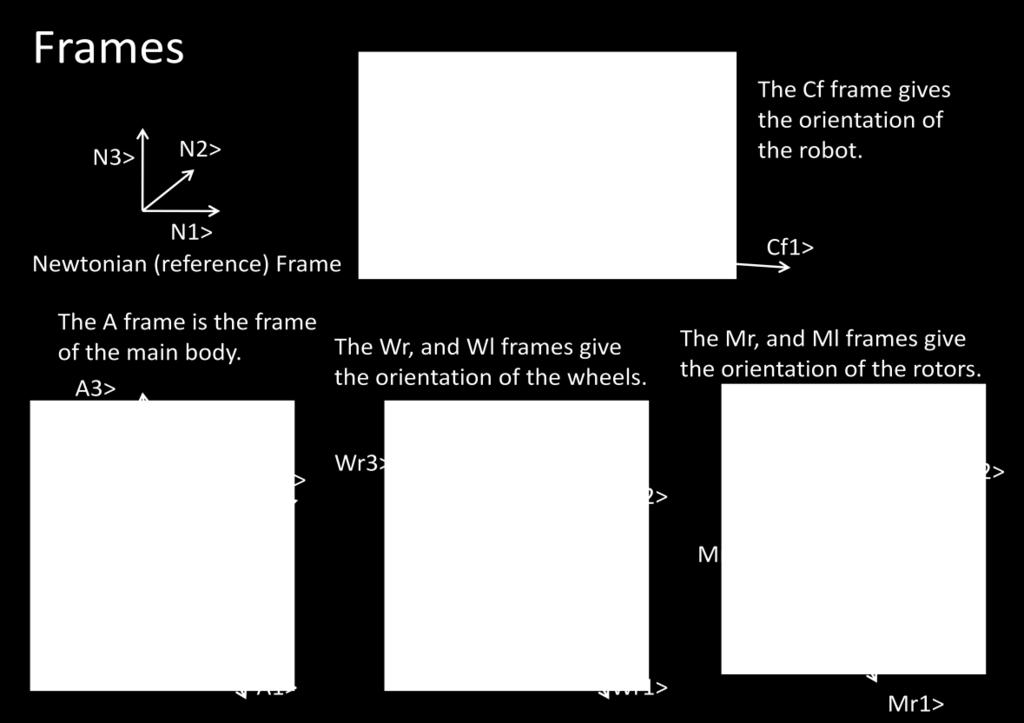
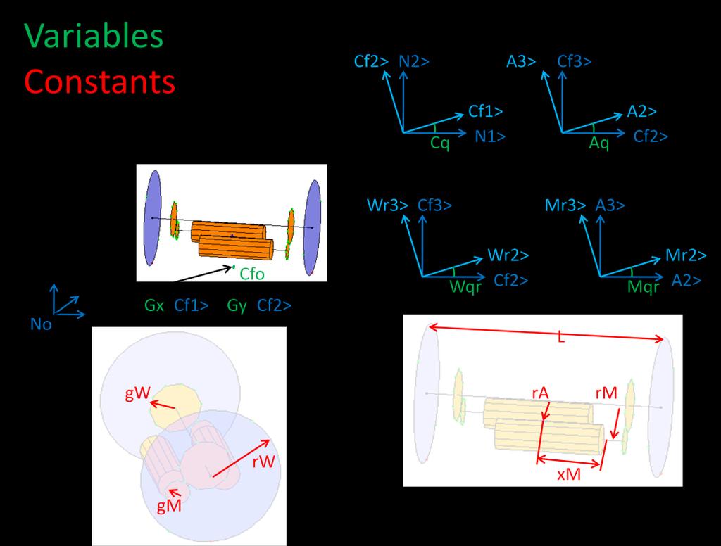
66 58

67 Autolev Model: % File: MPCredo.al % Date: March 3, 2010 % Author: Eric Olson % Problem: This is a simulation of a robot with a wheel at ether % of a central body. It moves by moving the central % body about the central axis. This moves the mass of % the robot off center and causes it to roll. % r = right, l = left % This simulation has the values for the bigger gear design. % % Default settings AutoEpsilon 1.0E-14 % Rounds off to nearest integer AutoZ OFF % Turn ON for large problems Digits 7 % Number of digits displayed for numbers % % Newtonian, bodies, frames, particles, points Newtonian N Frames Cf % Frame used to define the contact force directions. Bodies Wr, Wl, A, Mr, Ml % Wheels, central body, and roter Points C % Central point of device Points Cr, Cl % Wheel contact point % % Variables, constants, and specified Variables Cx', Cy' % distance from No to the center of the robot (not its CG) Variables Wqr', Wql' % Angle between frames Cf and W Variables Mqr', Mql' % Rotor angles Variables Cq', Aq' % Angle between N and Cf, Angle between frames Cf and A Constants Grav % Local gravitational acceleration Constants rw % Radius of wheels Constants ra % Distance of Ao from central axis Constants L % Distance between Wro and Wlo Constants xm, rm, qm % Position of the rotors Constants gm, gw % rotor and wheel gear radius Variables Tr, Tl % Torque on wheels % Specified Ff, Fftr, Fftl % Ff -Friction force out of the plane of the wheel, Fft - Friction force tangent to the wheel % % Motion variables for static/dynamic analysis Variables u{8}' % Motion variables; derivatives Cx' = u1 Cy' = u2 59

68 Aq' = u3 Cq' = u4 Wqr' = u5 Wql' = u6 Mqr' = u7 Mql' = u8 % % Mass and inertia properties Mass A=mA, Wr=mW, Wl=mW, Mr=mM, Ml=mM Inertia A, IA11, IA22, IA33 Inertia Wr, mw*rw^2/2, mw*rw^2/4, mw*rw^2/4 Inertia Wl, mw*rw^2/2, mw*rw^2/4, mw*rw^2/4 Inertia Mr, IML, IMR, IMR Inertia Ml, IML, IMR, IMR % % Geometry relating unit vectors Simprot(N, Cf, 3, Cq) Simprot(Cf, A, 1, Aq) Simprot(A, Wr, 1, Wqr) Simprot(A, Wl, 1, Wql) Simprot(A, Mr, 1, Mqr) Simprot(A, Ml, 1, Mql) % % Angular velocities W_Cf_N> = Cq'*N3> W_Wr_A> = Wqr'*A1> W_Wl_A> = Wql'*A1> W_A_Cf> = Aq'*Cf1> W_Mr_A> = Mqr'*A1> W_Ml_A> = Mql'*A1> % % Position vectors % There are three ways to define P_No_C>: %P_No_C> = Cx*N1> + cy*n2> + rw*n3> % This works, but the simulation gives wornings about close to singulare matracies, it keeps going though. P_No_C> = Cx*Cf1> + cy*cf2> + rw*cf3> % This seems to work best. P_C_Ao> = -ra*a3> P_C_Wro> = (1/2)*L*A1> P_C_Wlo> = -(1/2)*L*A1> P_Wro_Cr> = -rw*cf3> P_Wlo_Cl> = -rw*cf3> P_C_Mro> = xm*a1> - rm*cos(qm)*a2> - rm*sin(qm)*a3> P_C_Mlo> = -xm*a1> + rm*cos(qm)*a2> - rm*sin(qm)*a3> 60

69 % % Velocities V_C_N> = Dt(P_No_C>,N) V_Ao_N> = Dt(P_No_Ao>,N) V_Wro_N> = Dt(P_No_Wro>,N) V_Wlo_N> = Dt(P_No_Wlo>,N) V_Cr_N> = Dt(P_No_Cr>,N) V_Cl_N> = Dt(P_No_Cl>,N) V_Mro_N> = Dt(P_No_Mro>,N) V_Mlo_N> = Dt(P_No_Mlo>,N) % % Motion constraints Dependent[1] = gw*dot(w_wr_a>,a1>) + gm*dot(w_mr_a>,a1>) Dependent[2] = gw*dot(w_wl_a>,a1>) + gm*dot(w_ml_a>,a1>) Dependent[3] = Dot(V_C_N>,Cf1>) % Wheels do not slip Dependent[4] = Dot(V_Wro_N> + Cross(W_Wr_N>,P_Wro_Cr>),Cf2>) % Wheel rotation Dependent[5] = Dot(V_Wlo_N> + Cross(W_Wl_N>,P_Wlo_Cl>),Cf2>) % Auxiliary[1] = Dot(V_C_N>,Cf1>) % Wheels do not slip % Auxiliary[2] = Dot(V_Wro_N> + Cross(W_Wr_N>,P_Wro_Cr>),Cf2>) % Wheel rotation % Auxiliary[3] = Dot(V_Wlo_N> + Cross(W_Wl_N>,P_Wlo_Cr>),Cf2>) % Auxiliary[2] = coef(express(v_wro_n>,cf),cf2>) + rw*wqr' % Auxiliary[3] = coef(express(v_wlo_n>,cf),cf2>) + rw*wql' % For some reason, this is different than the above value. Constrain(Dependent[u7,u8,u1,u5,u6]) % Constrain(Dependent[u7,u8],Auxiliary[u1,u5,u6]) Pause % % Angular accelerations ALF_Cf_N> = Dt(W_Cf_N>,N) ALF_Wr_N> = Dt(W_Wr_N>,N) ALF_Wl_N> = Dt(W_Wl_N>,N) ALF_A_N> = Dt(W_A_N>,N) ALF_Mr_N> = Dt(W_Mr_N>,N) ALF_Ml_N> = Dt(W_Ml_N>,N) % % Accelerations A_C_N> = Dt(V_C_N>,N) A_Wro_N> = Dt(V_Wro_N>,N) 61

70 A_Wlo_N> = Dt(V_Wlo_N>,N) A_Ao_N> = Dt(V_Ao_N>,N) A_Cr_N> = Dt(V_Cr_N>,N) A_Cl_N> = Dt(V_Cl_N>,N) A_Mro_N> = Dt(V_Mro_N>,N) A_Mlo_N> = Dt(V_Mlo_N>,N) % % Forces Gravity(-Grav*N3>) % Force_C> += Ff*Cf1> % Force_Cr> += Fftr*Cf2> % Force_Cl> += Fftl*Cf2> % % Torques Torque(A/Mr,Tr*A1>) Torque(A/Ml,Tl*A1>) % Torque(A/Mr,(Tr-Fq*Mqr)*A1>) % Torque(A/Ml,(Tl-Fq*Mql)*A1>) % Torque_Wr> += Fftr*rW*Cf1> % I'm not sure this should be included. % Torque_Wl> += Fftl*rW*Cf1> % % Equations of motion Zero = Fr() + FrStar() % Find equations of motion Kane() % CNx = coef(express(p_no_c>,n),n1>) CNy = coef(express(p_no_c>,n),n2>) CNz = coef(express(p_no_c>,n),n3>) CVx = coef(express(v_c_n>,n),n1>) the system CVy = coef(express(v_c_n>,n),n2>) CVz = coef(express(v_c_n>,n),n3>) % Point Coordinates in Frame N Wrx = Dot(P_No_Wro>,N1>) Wry = Dot(P_No_Wro>,N2>) Wrz = Dot(P_No_Wro>,N3>) Crx = Dot(P_No_Cr>,N1>) Cry = Dot(P_No_Cr>,N2>) Crz = Dot(P_No_Cr>,N3>) % Center of the system % Velocity of the center of % Center of the right wheel % Right wheel contact point 62

71 Wrx0deg = Dot(P_No_Wro> + rw*wr2>,n1>) right wheel Wry0deg = Dot(P_No_Wro> + rw*wr2>,n2>) Wrz0deg = Dot(P_No_Wro> + rw*wr2>,n3>) % A point at the edge of the Wrx180deg = Dot(P_No_Wro> - rw*wr2>,n1>) % A point at the edge of the right wheel Wry180deg = Dot(P_No_Wro> - rw*wr2>,n2>) Wrz180deg = Dot(P_No_Wro> - rw*wr2>,n3>) Wgrx = Dot(P_No_C> + (xm+0.1*l)*wr1>,n1>) % Center of right wheel gear Wgry = Dot(P_No_C> + (xm+0.1*l)*wr1>,n2>) Wgrz = Dot(P_No_C> + (xm+0.1*l)*wr1>,n3>) Mrx = Dot(P_No_Mro>,N1>) Mry = Dot(P_No_Mro>,N2>) Mrz = Dot(P_No_Mro>,N3>) Wlx = Dot(P_No_Wlo>,N1>) Wly = Dot(P_No_Wlo>,N2>) Wlz = Dot(P_No_Wlo>,N3>) Clx = Dot(P_No_Cl>,N1>) Cly = Dot(P_No_Cl>,N2>) Clz = Dot(P_No_Cl>,N3>) Wlx0deg = Dot(P_No_Wlo> + rw*wl2>,n1>) left wheel Wly0deg = Dot(P_No_Wlo> + rw*wl2>,n2>) Wlz0deg = Dot(P_No_Wlo> + rw*wl2>,n3>) Wlx180deg = Dot(P_No_Wlo> - rw*wl2>,n1>) wheel Wly180deg = Dot(P_No_Wlo> - rw*wl2>,n2>) Wlz180deg = Dot(P_No_Wlo> - rw*wl2>,n3>) % Right rotor % Center of the left wheel % Left wheel contact point % A point at the edge of the % A point at the edge of the left Wglx = Dot(P_No_C> - (xm+0.1*l)*wr1>,n1>) % Center of left wheel gear Wgly = Dot(P_No_C> - (xm+0.1*l)*wr1>,n2>) Wglz = Dot(P_No_C> - (xm+0.1*l)*wr1>,n3>) Mlx = Dot(P_No_Mlo>,N1>) Mly = Dot(P_No_Mlo>,N2>) Mlz = Dot(P_No_Mlo>,N3>) % Left rotor 63

72 Ax = Dot(P_No_Ao>,N1>) Ay = Dot(P_No_Ao>,N2>) Az = Dot(P_No_Ao>,N3>) % CG of the central body % % Check Check = NiCheck() % % Units system for CODE input/output conversions UnitSystem kg,meter,sec % % Integration parameters and values for constants and variables Input tfinal=4, integstp=0.02, abserr=1.0e-08, relerr=1.0e-08 Input Grav=9.81 m/sec^2, rw= m, ra=0.004 m, L=0.045 m % Input constants Input xm = m, rm = m, qm=pi/4 rad Input gm= m, gw= m Input ma=0.015 kg, mw=0.002 kg, mm= kg Input IA11=7.0-7 kg*m^2, IA22=2.0e-6 kg*m^2, IA33=1.5e-6 kg*m^2 Input IML=5e-10 kg*m^2, IMR=5e-10 kg*m^2 Input Cx=0.005 m, Cy=0.005 m, u2=0 m/sec % Initial values Input Wqr=0 rad, Wql=0 rad, Mqr=0 rad, Mql=0 rad Input Cq=0 rad, Aq=0 rad, u3=0 rad/sec, u4=0 rad/sec Input Tr=0.8e-5 newtons*m, Tl=0.8e-5 newtons*m Input WCheck1=0 newton*m % % Quantities to be output from CODE Output Check newton*m, t sec, Aq deg, Cq deg % 1 Output t sec, CNx m, CNy m, CNz m % 2 Output t sec, Cq rad, Aq rad, Wqr rad, Wql rad, & % 3 Mqr rad, Mql rad, Cx m, Cy m, & u2 m/sec, u3 rad/sec, u4 rad/sec Output t sec, Ax m, Ay m, Az m, Wrx m, Wry m, Wrz m, & % 4 Wlx m, Wly m, Wlz m, Mrx m, Mry m, Mrz m, & Mlx m, Mly m, Mlz m Output t sec, Wrx0deg m, Wry0deg m, Wrz0deg m, & % 5 Wrx180deg m, Wry180deg m, Wrz180deg m, & Wlx0deg m, Wly0deg m, Wlz0deg m, & Wlx180deg m, Wly180deg m, Wlz180deg m, & Crx m, cry m, Crz m, Clx m, Cly m, Clz m, & Wgrx m, Wgry m, Wgrz m, Wglx m, Wgly m, Wglz m Output rw m, ra m, L m, xm m, rm m, qm m, gm m, gw m % 6 Output t sec, Tr newtons*m, Tl newtons*m % 7 % Output t sec, Ff newtons, Fftr newtons, Fftl newtons % 8 %

73 % Matlab code generation for numerical solution Code dynamics() MPCredo.m 65

74 APPENDIX C SIMPLIFIED AUTOLEV DYNAMIC MODEL 66

75 This is the Autolev code used to develop the dynamic model that was the basis for all the control development and simulation presented in this paper. This model is similar to the previous one except that the body does not have the freedom to rotate about its axis, and the wheel constraints are simplified to slider constraints. Autolev Model: % File: SimplifiedForControl.al % Date: January 26, 2010 % Author: Eric Olson % Problem: This is a simplified model for control development. % % Default settings AutoEpsilon 1.0E-14 % Rounds off to nearest integer AutoZ OFF % Turn ON for large problems Digits 7 % Number of digits displayed for numbers % % Newtonian, bodies, frames, particles, points Newtonian N Bodies A Points Ar, Al % % Variables, constants, and specified Variables Gx', Gy' % distance from No to Ao Variables Cq' % Angle between N and Cf Variables Fr, Fl % Forces acting on A Constants L % Length of A Constants xm, rm, qm % Position of the rotors Specified Ff % Friction force that keeps A from moving axialy % % Motion variables for static/dynamic analysis Variables u{3}' % Motion variables; derivatives Gx' = u1 Gy' = u2 Cq' = u3 % % Mass and inertia properties Mass A=mA Inertia A, IA11, IA22, IA33 % % Geometry relating unit vectors 67

76 Simprot(N, A, 3, Cq) % % Angular velocities W_A_N> = Cq'*N3> % % Position vectors P_No_Ao> = Gx*A1> + Gy*A2> P_Ao_Ar> = 0.5*L*A1> P_Ao_Al> = -0.5*L*A1> % % Velocities V_Ao_N> = Dt(P_No_Ao>,N) V_Ar_N> = Dt(P_No_Ar>,N) V_Al_N> = Dt(P_No_Al>,N) % % Motion constraints Auxiliary[1] = coef(express(v_ao_n>,a),a1>) Constrain(Auxiliary[u1]) Pause % % Angular accelerations ALF_A_N> = Dt(W_A_N>,N) % % Accelerations A_Ao_N> = Dt(V_Ao_N>,N) A_Ar_N> = Dt(V_Ar_N>,N) A_Al_N> = Dt(V_Al_N>,N) % % Forces Force_Ao> = Ff*A1> Force_Ar> = Fr*A2> Force_Al> = Fl*A2> % % Equations of motion Zero = Fr() + FrStar() % Find equations of motion Kane(Ff) % Simplify and/or solve % % Point Coordinates in Frame N Ax = coef(express(p_no_ao>,n),n1>) Ay = coef(express(p_no_ao>,n),n2>) Az = coef(express(p_no_ao>,n),n3>) % CG of A % Does not slip AVx = coef(express(v_ao_n>,n),n1>) AVy = coef(express(v_ao_n>,n),n2>) 68 % CG of A

77 AVz = coef(express(v_ao_n>,n),n3>) Axr = coef(express(p_no_ar>,n),n1>) Ayr = coef(express(p_no_ar>,n),n2>) Azr = coef(express(p_no_ar>,n),n3>) % Right end Axl = coef(express(p_no_al>,n),n1>) % Left end Ayl = coef(express(p_no_al>,n),n2>) Azl = coef(express(p_no_al>,n),n3>) % % Check Check = NiCheck() % % Units system for CODE input/output conversions UnitSystem kg,meter,sec % % Integration parameters and values for constants and variables Input tfinal=5, integstp=0.02, abserr=1.0e-08, relerr=1.0e-08 Input L=0.045 m % Input constants Input ma=0.015 kg Input IA11=7.0-7 kg*m^2, IA22=2.0e-6 kg*m^2, IA33=1.5e-6 kg*m^2 Input Gx=0.000 m, Gy=0.000 m, u2=0 m/sec % Initial values Input Cq=0 rad, u3=0 rad/sec Input Fr=0.0e-4 newtons, Fl=0.0e-4 newtons Input WCheck1=0 newton*m Input Axd=0.1 m, Ayd=0.1 m % % Quantities to be output from CODE Output Check newton*m, t sec, Cq deg % 1 Output t sec, Cq rad, L m % 2 Output t sec, Ax m, Ay m, Az m, Axr m, Ayr m, Azr m, & % 3 Axl m, Ayl m, Azl m, AVx m, AVy m, AVz m Output t sec, Fr newtons, Fl newtons, Ff newtons % 4 Output t sec, Axd m, Ayd m % 5 % % Matlab code generation for numerical solution Code dynamics() SimplifiedForControl.m 69

78 APPENDIX D CONTROLLER STABILITY 70

79 From section 2.3.1, it was shown that the derivative of the Lyapunov function (16) using the proposed controller could be simplified to equation (23). From the Autolev program, the equations of motion for this dynamic model are, Or in the standard form, Equations (11), (12), and (15) show that, Therefore, Substituting this into equation (23) gives, The first and last terms in this equation are obviously negative, however to show that the middle term is negative, it is necessary to find the relationship between and. This will be accomplished using the relationships between,, and. 71

80 From this Figure it is apparent that, This equation applies as long as and do not equal zero. It should be noted that and will never become zero while the controller is in effect since an area is defined around the desired point in which the controller does not take effect, as is stated in sections and Taking the derivative of this and rearranging the terms results in an expression that relates and. 72

81 Again using the relation, this equation becomes, Substituting this back into the expression for yields, If the desired point is restated through some transformation as the origin of a new coordinate system, then. The error in the direction and then be rewritten as. Using this, and the relation, can be farther rearranged to, This equation can be rearranged farther to, From this, it is apparent that is always negative, that is energy will be subtracted from the system and the system will eventually reach the goal in a stable manner. 73

82 APPENDIX E PARTS UTILIZED 74

83 This is a list of all the off-the-shelf parts that went into the robot. Product Part Number Price Quantity Micro Planetary Gear Motor GH6123 $16 2 Qik Dual Serial Motor Controller ROB $25 1 Bluetooth SMD Module - Roving Networks WRL $30 1 Polymer Lithium Ion Batteries - 100mAh PRT $7 1 Motor Gear GM $2 2 Spur Gear GS $ " Micro Sport Wheels 2pc $2 1 75

84 APPENDIX F WIRING DIAGRAM 76

85 This is the wiring schematic used to connect all the electrical components used in the robot. The motors are connected only to the motor control board. All the components accept the same voltage. 77

86 APPENDIX G LABVIEW GUI 78

87 his shows the front end of the LabVIEW program. All the various controls can be seen on the right. 79

88 APPENDIX H EXAMPLE LABVIEW CODE 80

89 In this section, more of the LabVIEW code is shown. This part of the program sets up the windows voice recognition software, and defines the recognized terms. This part of the program does vision calibration. 81

90 This part of the program finds the robot and locates it relative to the reference frame. This program initializes the Bluetooth connection. This program takes the mouse user input to generate a desired location for the robot. 82

91 This is the feedback part of the program. 83

92 This is the PD control VI. This is the path planning coefficient VI This is the time dependent part of the path generation. 84

93 APPENDIX I SETUP 85

94 This is the basic setup for the robot. There is a workspace, which the robot drives on, with calibration images, and there is a camera, which is used for position feedback, looking down on the workspace. 86