Experimental Modal Analysis of an Automobile Tire

Transcription

1 Experimental Modal Analysis of an Automobile Tire J.H.A.M. Vervoort Report No. DCT Bachelor final project Coach: Dr. Ir. I. Lopez Arteaga Supervisor: Prof. Dr. Ir. H. Nijmeijer Eindhoven University of Technology (TU/e) Department of Mechanical Engineering Dynamics and Control Technology Group Eindhoven, May, 2007

2

3 Abstract This project will continue an earlier performed study on the experimental modal analysis of an automobile tire, see reference [6]. The standard automobile tire (type 205/60 R 15) with 1.6 bar pressure is hanged in three elastic strips within a specially designed frame, to provide a free suspended condition for the tire. When the tire is excited at resonant frequencies, it vibrates in special shapes called mode shapes. By understanding the mode shapes, all possible types of vibration can be predicted, see reference [12]. The excitation is realized by an electro-dynamic shaker and the input force of the shaker is measured by a force transducer. An accelerometer measures the response at several points on the tire and a dynamic signal analyzer computes the frequency response functions (FRFs). The tire is measured with enough points to see the first six mode shapes and does not use a grid pattern to measure the tire, but only the circumference and one crosssection of the tire. With these two measurement lines the behavior of the complete tire is estimated. The change of the modal amplitude in the circumference and cross-section is used to estimate the missing points of the grid. The first six natural frequencies of the tire are clearly visualized. The resonances have the following natural frequencies: 114 Hz, 137 Hz, 165 Hz, 196 Hz, 228 Hz and 260 Hz. The cross-section measurements of the tire are of moderate quality. This is caused by the less effective attachment of the accelerometer. The moderate quality of the crosssection also causes the estimation of the complete tire to be of a moderate quality. In future work, methods to improve the attachment of the accelerometer to the tire need to be investigated. i

4 List of symbols Symbol Definition Unit T N f s f max f F x(t) y(t) X(f) Y(f) S xx (f) S xy (f) S yy (f) H xy (f) Υ 2 xy(f) Record length Record length used by Siglab Sampling frequency Maximum frequency Spectral density Frequency resolution used by Siglab Input signal in time domain Output signal in time domain Input signal in frequency domain Output signal in frequency domain Auto power spectrum (input) Cross power spectrum Auto power spectrum (output) Frequency response function estimator Coherence function Sec Lines Hz Hz Hz Hz ii

5 Table of contents Abstract List of symbols Table of contents i ii iii 1 Introduction An automobile tire and modal analysis Goals and outline 2 2 Experiments The method and setup used for the experiments The experiments and measuring points Measuring equipment The shaker The force transducer The accelerometer The dynamic signal analyzer Frequency response functions Auto / cross - power spectrum Coherence 11 3 Measurement quality Quality improvement Input range Frequency range Triggering Windowing Averaging Quality check Repeatability and reproducibility Driving point measurements 15 4 Modal Analysis Modal parameter estimation Number of modes Estimation method Mode shapes Tread side or circumference of the tire Cross-sections of the tire Estimation of the complete tire 21 5 Evaluation A half or quarter circumference measurement of the tire 24 iii

6 5.2 A complete or half cross-section measurement of the tire The influence of the accelerometer attachment and the comparison of the 26 different sides of the tire 5.4 The estimation of the complete tire Evaluation of the complete tire modulation Checking the first Matlab model with the data of the measured crosssection 35 at 90 degrees from the excitation point 6 Conclusion 38 7 Recommendations 40 Appendix: A Specifications of the measurement equipment 41 A1 The shaker 41 A2 The force transducer 41 A3 The accelerometer 41 A4 The dynamic signal analyzer 41 B Measurement points on the tire 42 B1 Tire s circumference 43 B2 Tire s sidewall 44 B3 Tire s cross-section at 0 degrees from the excitation point 45 B4 Tire s cross-section at 90 degrees from the excitation point 45 B5 Tire s cross-section at 180 degrees from the excitation point 45 C Mode indicator functions 46 D Estimated mode shapes of the tire s circumference 49 E Estimated mode shapes of the tire s side wall 52 F Estimated mode shapes of the tire s cross-sections 55 G Matlab model 62 H Results of Matlab model one, direct use of measurement data 68 I Results of Matlab model two, use of ME scope fitted data 72 J Comparison of the cross-section at 90 degrees with the complete tire model 81 8 Bibliography 82 iv

7 Chapter 1 Introduction The experimental modal analysis of an automobile tire is the subject of this bachelor final project at Eindhoven University of Technology. The experimental modal analysis is performed to obtain the modal parameters of an automobile tire. The modal parameters can be used to tune a finite element model, which for the matter of fact is not done in this project. The finite element model greatly aids in the design of the tire by predicting its vibration response. 1.1 An automobile tire and modal analysis The automobile tire is an important source of vibration and noise inside the vehicle. To improve the tire s influence on the vehicle, one has to know how the tire behaves. This behavior is stored in the tire s dynamic properties which can be researched. When the frequency response function (FRF) of a point on the tire is measured, one knows how this point on the tire responses too a certain frequency input. When the tire is excited at resonant frequencies, it vibrates in special shapes called mode shapes. Under normal circumstances, the tire will vibrate in a complex combination of all mode shapes. By understanding the mode shapes, all possible types of vibration can be predicted, see reference [12]. By experimental modal analysis, the mode shapes can be measured together with the modal frequency and modal damping. Experimental modal analysis consists of: exciting the tire with an electro-dynamic shaker, measuring the FRFs between the excitation and numerous points on the tire, and then using software to visualize the mode shapes. This project will continue an earlier performed study of the experimental modal analysis of an automobile tire, see reference [6]. The standard automobile tire (type 205/60 R 15) with 1.6 bar pressure is hanged in three elastic strips within a specially designed frame, to provide a free suspended condition for the tire. The strips have a very low natural frequency which ensures the free-free condition. More information about the tire can be found in appendix B. 1

8 In the previous study, the tire is divided into a grid pattern that covers half of the tire. The size of the grids determines the accuracy of the measurements. But in this previous study the tire is measured with too little grid points to see at least six mode shapes within the circumference of the tire. In this project the tire is measured with enough points to see these six mode shapes and does not use the grid pattern to measure the tire, but only the circumference and one cross-section of the tire. By these two measurement lines the behavior of the complete tire can be predicted. 1.2 Goals and outline To measure the tire s first six mode shapes, the tire has to be measured with enough points. Measuring the complete tire with enough points costs a lot of time. The previous study revealed that by measuring only half of the tire, the behavior of the complete tire can be predicted. This means measuring time is cut in half, but maybe it is possible to shorten the measurement time even more. This is why the first goal is: to see if it is possible to shorten the measurement time. The second and most important goal is to measure the tire s first six mode shapes and obtaining the modal parameters, with the first goal in mind. The measurements need to be performed in the shortest possible measurement time. This is why the complete tire is estimated with only one cross-section and circumference. This report is divided into the five following subjects. First, the experiments with: the experimental setup, the measurement points, the measuring equipment and an explanation of the estimation of the FRF, are discussed in chapter 2. Then, the measurement quality which is an important part of experimental modal analysis is discussed in chapter 3. After that, the modal parameter estimation and the experimental results is discussed in chapter 4. Fourth, the evaluations of these results are discussed in chapter 5 and finally the conclusion and recommendation are discussed in chapter 6 and 7. 2

9 Chapter 2 Experiments Experiments need to be performed to obtain the FRFs needed for the modal analysis of an automobile tire. This chapter deals with the explanation of the method and setup used for the experiments, which measurement equipment is used, and how FRFs are estimated. 2.1 The method and setup used for the experiments To obtain the FRFs of an automobile tire, the response of the tire to a point excitation has to be measured. The excitation is realized by an electro-dynamic shaker and the input force of the shaker is measured by a force transducer. An accelerometer measures the response at several points on the tire and a dynamic signal analyzer computes the FRFs. A FRF is made for every point measured on the tire. The number of measurement points determines the accuracy of the mode shape, which is explained in the next subsection. Each FRF represents the resonant frequencies of the tire and the modal amplitudes of its specific point. The amplitude of the FRFs indicates the ratio of the acceleration divided by the input force, see equation 2.1, and see also reference [1]. Response = Tire properties * Input (eq. 2.1) The automobile tire as explained in the introduction is tested in a free condition. This means that the tire is not attached to the ground at any of its coordinates. In practice it is not possible to make a truly free support but it is feasible to provide a suspension system which closely approximates to the free condition. That is why the tire is hanged in three light elastic strips as can be seen in figure 2.1 below, see reference [1] for more information about free supports. The elastic strip attached at the top is thicker because it needs to hold the tire s weight. The two other elastic strips are used to keep the tire straight. As can be seen in 3

10 figure 2.1 the electro-dynamic shaker is also hanged elastically to ensure the free-free condition of the tire. Steel frame Elastic strip Accelerometer Siglab Laptop Amplifier Shaker Force transducer Tire Mountingring Figure 2.1: FRF measurement setup The experiments and measuring points Three different experiments are needed to accomplish the goals of this project; these goals are mentioned in the introduction. The first experiment investigates the possibility to measure only a quarter of the tire s circumference and half cross-section, to shorten measurement time. This is done by measuring the tire s half circumference and comparing the results of the two quarters in it. If this is possible more measuring points can be taken of the quarter of the tire, so a clearer image of the tire will be the result. The same is done for the tire s cross-section, though the cross-section is completely measured and the two halves in it compared. The tire s half circumference is measured with 24 points, the coordinates of these points can be found in appendix B. The tire s cross- 4

11 section is measured with 11 points at 180 degrees from the excitation point; the excitation point is point number 1 of the circumference. The coordinates of the tire s cross-section points can also be found in appendix B. The second experiment takes the main goal of this project into account. The tire s modal parameters need to be obtained and the tire needs to be measured with enough points to see the first six mode shapes within the desired bandwidth of 0 to 500 Hz. In the previous study the tire is divided into a grid pattern that covers half of the tire. The size of the grid determines the accuracy of the measurements. It takes a lot of time to measure the complete grid. Because measurement time has to be shortened according to the first goal, only the circumference and one cross-section of the tire are measured. The change of the modal amplitude in the circumference and cross-section is used to calculate the missing points of the grid. The circumference and cross-section are measured with more points, if they are measured with the same amount of points, as the tire would be with the use of a grid. This results in more accurate mode shapes, or if the accuracy admits lesser points are measured and measurement time is shortened. Section 4.3 provides more information about the use of one cross-section and circumference. To obtain a smooth mode shape it is important to measure the tire with enough measurement points. The more points, the smoother the mode shapes but the more time it costs to complete the experiment. Every mode shape can be described in terms of an integer number of wavelengths along the circumference; the tire s sixth mode shape has seven wavelengths within the tire. Every wavelength should have at least six measurement points for a smooth visualization. Experiment one determines how in experiment two the tire s mode shapes and modal parameters are estimated. This can be done with the measurement of the half or quarter circumference and the complete or half cross-section. The results of experiment one are described in chapter 4 and discussed in chapter 5. The conclusion that could be drawn is that the half circumference and the half cross-section have to be measured for an accurate closure of experiment two. That is why the tire s half circumference is measured with 24 points, which is enough for a smooth visualization. The tire s half cross-section is measured with 7 points, because every mode shape has one and a half wavelengths within 5

12 the cross-section. The coordinates of the measurement points of the circumference and the cross-section are presented in Appendix B. For experiment two, the cross-section at 0 degrees from the excitation point is used, because the vibrations provided by the electrodynamic shaker are not damped yet. The third experiment measures a second cross-section of the tire at 90 degrees from the excitation point. This cross-section is measured to check if the model calculates the points on the grid correctly. If the model calculates the points correct the difference between the calculated points and the measured points should be minimal. The measurement points of this cross-section are also represented in Appendix B. A chirp type signal is chosen to excite the tire. For one measurement the chirp runs from 0 to 500 Hz in one second. After this second there is a one second pause before a next chirp is started for the next measurement. In the pause the chirp dies out, so the next measurement is not corrupted by the previous chirp. One point is measured 50 times with a chirp signal and averaged. More information about the frequency range, averaging and other measurement settings can be found in chapter 3. The software which provides the demanded chirp and measures the response of the tire is named Siglab. More information about this software can be found in references [2] and [3]. After the measured data is saved, the modal parameters are calculated with a different software program named ME scope. More information about ME scope can be found in reference [4]. 6

13 2.2 Measuring equipment In the experiments explained above measuring equipment provides the demanded input and output data. In this section the measuring equipment will be described to give a better understanding of the experiments. The measuring equipment consists of: an electro-dynamic shaker, a force transducer, an accelerometer and a dynamic signal analyzer, as can be seen on figure 2.1 in the previous section The shaker Figure 2.2: The electro-dynamic shaker The electro-dynamic shaker (see figure 2.2) is used to give the tire an excitation which is prescribed by Siglab and amplified by an amplifier. The electro-dynamic shaker is connected through a stinger with a force transducer. A stinger is a small metal wire which is stiff in one direction and flexible in all the other. The electro-dynamic shaker is hanged elastically, so external noise is damped as explained in section 2.1. When elastically hanged the electro-dynamic shaker also gives itself an excitation, but this does not matter, because the force transducer only measures the resulting force, and the prescribed frequency is not changed. The specifications of the electro-dynamic shaker are represented in appendix A. 7

14 2.2.2 The force transducer Figure 2.3: The force transducer, attached to the tire The force transducer (see figure 2.3) is used to measure the force of the excitation brought by the electro-dynamic shaker. It is attached to the tire with a screw, which fits in the profile of the tire. Siglab powers the force transducer with an automatically chosen constant voltage (type bias). The output signal of the force transducer runs through the same cable and is present as a voltage modulation. The specifications of the force transducer are represented in appendix A The accelerometer Figure 2.4: The accelerometer The accelerometer (see figure 2.4) is used to measure the acceleration of different points on the tire. It is attached to the tire with a thin layer of mounting wax, or is placed 8

15 between the tire s profile. It has a built-in charge amplifier and a low-impedance voltage output. The amplifier in the accelerometer is directly fed from Siglab, using a bias type of voltage. The specifications of the accelerometer are represented in appendix A The dynamic signal analyzer Figure 2.5: The dynamic signal analyzer The measurement of the force and acceleration signal is performed by the dynamic signal analyzer. The dynamic signal analyzer is a four channel Siglab analyzer, which samples the voltage signals coming from the force transducer and the accelerometer. The sensitivity information of the sensors is used to convert the voltages to equivalent force and acceleration signals. It is also used to transform these time domain signals into a FRF. The transformation from the time domain signals into a FRF is invisible for the user. In subsection 2.3 the basic idea of this transformation is explained. The specifications of the dynamic signal analyzer are represented in appendix A. 9

16 2.3 Frequency response functions The measured FRFs quality directly determines the quality of modal parameters. This is why the estimation of the FRF is an important process of modal analysis. The estimation of this FRF is performed inside the dynamic signal analyzer and is invisible for the user. The basic ideas of the estimation are explained in the next subsections. More information about the estimation of the FRF can be found in references [7], [8], [9] and [13] Auto / cross - power spectrum The in time domain recorded input and response signals x(t) and y(t) are transformed into the frequency domain using the Fast Fourier Transformation. The frequency domain signals, referred as X(f) and Y(f), are used to calculate the auto and cross power spectrum. The auto spectrum of the input, referred as S xx (f), and the cross power spectrum of the input and output, referred as S xy (f), are formulated in equations 2.2 and * S xx ( f ) = X ( f ) X ( f ) (2.2) T 1 * S xy ( f ) = X ( f ) Y ( f ) (2.3) T * indicates the complex conjugate and T the measured time record length The auto power spectrum provides information about the frequencies that are present in the input signal, and about the contribution of each component to the total power in the signal. In contrast to the auto power spectrum, the cross power spectrum is a complex function. With the auto power spectrum and the cross power spectrum, the FRF [H xy (f)] can be estimated using equation (2.4). 10

17 S xy ( f ) H xy ( f ) = (2.4) S ( f ) xx The FRF contains both magnitude and phase information. The magnitude is typically shown on a logarithmic Y axis in db scale, and the phase is often shown on a 0 to 360 degree scale. However, since the phase often has shifts in degrees the discontinuities can be removed with use of phase unwrapping Coherence The coherence function is used to determine the quality of the estimated FRF. The coherence is formed when the cross power spectrum is normalized using the corresponding auto power spectra and is defined in equation (2.5). The coherence function is a normalized coefficient of correlation between the excitation signal x(t) and the response signal y(t) evaluated at each frequency. 2 S ( ) 2 xy f γ xy ( f ) = (2.5) S ( f ) S ( f ) xx yy The coherence function shows for each frequency which part of the response y(t) is caused by the input x(t). The range of the coherence function can be described by equation 2.6. If the value of the coherence is near one a linear relation exist between the input x(t) en the response y(t) and there is no influence of noise. In the other way if the value is near zero the response is dominated by the noise. 2 0 γ xy ( f ) 1 (2.6) γ = 1... S ( f ) << S ( f ) 2 xy nn yy γ = 0... S ( f ) >> S ( f ) 2 xy nn yy 11

18 Chapter 3 Measurement quality The quality of the measurement is very important and always requires attention in experiments. The quality depends on the sensors used, the dynamic signal analyzer and the skill of the person doing the experiments. In the next subsections, the influence of Siglab on the measurement quality, the reproducibility and driving point measurement are discussed. 3.1 Quality improvement Siglabs settings influence the accuracy of the measurement; they are represented by the following aspects: the input range, the frequency range, triggering, windowing and averaging. In the next subsections these aspects are explained Input range The input range can be specified by Siglab varying from 20 mv to 10V, and can be set for each channel. The range should be as small as possible because a smaller range means a higher resolution. If the input range is too large the analogue to digital conversion results in a coarse resolution which leads to large quantization errors (quantization noise). When the range is too small the amplitude of the incoming signal is larger than the maximum allowed value and an overload will occur. More information about quantization can be found in reference [12] The type of voltage can also be specified for every channel. The force transducer needs an external amplifier to collect data and the accelerometer receives power from Siglab, both need a bias type of voltage Frequency range Siglab provides two settings for the frequency range, the bandwidth and the record length. The minimal bandwidth needed for this experiment is 300 Hz (determined 12

19 in an earlier performed study, see reference [6]), but the nearest bandwidth that can be set in Siglab is 500 Hz. The record length in lines is set to 2048 lines. The ultimate frequency resolution of the analysis can be calculated using equation 3.1 and 3.2, where f max is the maximum frequency, f s is the sampling frequency and N is the record length in lines. Siglab s sampling frequency is always given by: f s = 2.56 * f max, further information can be found in reference [2]. 2.56* f max F = (3.1) N f s F = (3.2) N Triggering Triggering is used to capture the entire excitation and response signal in a sampling window. Siglab makes four parameters relevant to ensure triggering for an input channel namely; the threshold, slope, filter and trigger delay. The threshold is a percentage of the peak value of the total impulse. This determines the amplitude of a signal at which the measurement will start. The slope determines if the measurement starts with a decaying or a growing signal. When a filter is applied all the data goes through an anti-aliasing filter before it is triggered. When a signal is already present these parameters ensure the measurement to start, but the trigger delay ensures that the entire signal is monitored. For all experiments done in this project, the threshold is set to 9% with a positive slope, with no filter and a trigger delay of -10% Windowing Windowing is the most practical solution to the leakage problem. Leakage occurs when measured signals do not drop to zero within the measurement time interval. To minimize the effects of leakage the measured signals are multiplied with a window function before a Fast Fourier Transformation (FFT) is applied. Another option is to ensure that the measured signal starts at zero and drops to zero at the end of the measurement time interval without the use of a window. 13

20 In the experiments a chirp signal is used. This is a fast sweep from low to high frequency within one sample interval of the analyzer, which is explained in subsection Triggering ensures that the measured signal starts at zero and a pause between two chirp signals ensures that the measured signal is zero at the end of the measurement time interval. The advantage of this option is that it is not necessary to use a window and no artificial damping is introduced to the FRFs Averaging Every measurement is contaminated by noise or is influenced by the person doing the experiments. The accuracy of a FRF is mainly determined by these effects. This can be improved by averaging measurements, which reduces the effect of random errors. However averaging does not have an effect on systematic errors as leakage. There are different types of averaging: peak hold, exponential, linear, ect. In these experiments a linear averaging method without overlap is used. This means that every measured FRF has the importance, when calculating the average. Overlap can only be used when the measured signals are mutually uncorrelated, which means that the signals have no specific relation to one and other. All the experiments in this project use a chirp signal which belongs to a transient class of signal where overlap is of no use, see reference [1]. In all experiments, every point is measured 50 times. The 50 measurements are averaged resulting in a FRF without random errors. 3.2 Quality check During the measurement process the quality of the measured FRFs can be evaluated using the coherence function, as explained in subsection The coherence function can only indicate the effects of random errors, the effects of bias errors can not be indicated. Therefore additional checks are needed, to ensure that the quality of the FRFs is sufficient. Also, certain FRFs should be re-measured from time to time, to check that neither the structure nor the measurement system has experienced any significant changes. The next subsections will discus these topics. 14

21 3.2.1 Repeatability and reproducibility The repeatability or reproducibility of the measured FRFs is an essential check for any modal test. Certain FRFs should be re-measured from time to time, to check if there are some significant changes to the experimental setup (the structure and the measurement system). If a measured FRF is not reproducible this can have several reasons, a few primary factors are nonlinearities, insufficient clamping stiffness and inconsistencies in the measurement directions of the excitation and response. In this project one point (Point number 1, see appendix B) is re-measured every time an experiment is performed. The FRF of this point is compared with earlier taken FRFs Driving point measurements The driving point measurement is used to get an indication of the quality of the measurement loop. This is realized by measuring the excitation and response at the same location on the tire. The driving point FRF has to fulfill the following requirements: all resonances should be separated by anti-resonances, phase differences larger than 180 cannot occur and the imaginary parts of the FRF should not change sign. If the driving point FRF does not meet the requirements this indicates that the measurement loop is of poor quality. Measurement point 1 of the tire s circumference 15

22 Chapter 4 Modal Analysis In the modal analysis of a tire the modal parameters are estimated from the measured FRFs. The estimation process of the modal parameters consists of estimating the number of modes in the frequency band, choosing the best modal parameter estimation method and calculating and forming the mode shapes of the tire. The modal parameter estimation process is clarified in section 4.1 and 4.2. Section 4.3 deals with explaining the estimation process of the complete tire (with the use of only the circumference and one cross-section of the tire). In this chapter the results of the estimation process are presented. The next chapter will deal with the evaluation of these results. 4.1 Modal parameter estimation The tire s modal parameters are estimated by curve fitting the measured FRFs. Curve fitting is performed by ME scope and has a set of modal parameters as outcome. The modal parameters contain the frequency, damping and mode shape for each eigenmode that is identified in the desired frequency range. The curve fitting process is completed in a two steps: determining the number of modes and applying the best estimation method. The estimation method is used to estimate the frequency, damping and residues in the desired frequency range Number of modes The first step in the modal parameter estimation process is estimating the number of modes in the desired frequency range, which start at 0 Hz and ends at 500 Hz, explained in subsection Estimating the number of modes in the measured FRFs can be done in several ways. However, in this report there are only two methods discussed. In the first method, all the FRFs of the tire are overlaid. In figure 4.1 all the FRFs of the tire s circumference are overlaid and in figure 4.2 the FRFs of the cross-section (at 16

23 0 degrees from the excitation point). All the FRFs have resonance peaks at the tire s eigenmodes frequencies, except if the measured point is a nodal point at that specific frequency. Figure 4.1: Overlay of the FRFs of the circumference Figure 4.2: Overlay of the FRFs of the cross-section 17

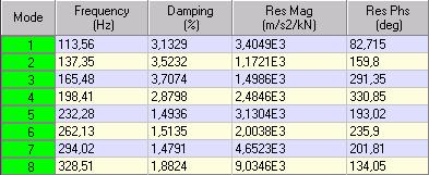
24 The second method to estimate the number of modes is by using a mode indicator function. The mode indicator function can be applied with ME scope, which offers three different methods, namely, the modal peaks function, the complex mode indicator function and the multivariate mode indicator function. More information about these three different methods can be found in references [4] and [6]. For all the experiments a modal peaks function is applied. The basic idea behind the modal peak function is that it sums the magnitudes of all the FRFs. This sum gives a mode indicator function where the peaks show the resonance or eigenmode frequencies. In appendix C the mode indicator function of the tire s circumference and cross-section is shown. The eigenmode frequencies at the peak values of the mode indicator function are highlighted by the vertical green lines Estimation Method The modal parameter estimation method estimates the frequency, damping and residues for each eigenmode that is identified. For the estimation process different methods can be chosen, which all have their own properties. There are three sorts of properties, namely: a single degree of freedom or a multiple degree of freedom, a local or a global method, and the frequency domain or the time domain. For all experiments the global polynomial method is chosen. Global polynomial method The polynomial method is a multi degree of freedom method that simultaneously estimates the modal parameters of two or more modes and uses a frequency domain curve fitting method. The fitting method utilizes the complex trace data in the cursor band for curve fitting. More information about the polynomial method can be found in reference [4]. The advantage of using a multi degree of freedom method is that it gives the best modal parameter estimates when the eigenmodes are close together and the damping is relatively high, which is for tires. The global method is chosen because it uses a formulation where all FRFs are considered simultaneously and curve fitted together. When doing so, a global modal 18

25 frequency and damping estimate results, this is one estimate of each resonance frequency and damping value. The global method requires a high quality of measurement data because it is sensitive for small variations. When the quality of measurement data is high enough the global method delivers superior results compared to the local method. More information about the global method can be found in references [4] and [8]. With the use of ME scope a global polynomial method can be used to fit the measured data of the tire. The global polynomial method estimates the frequency, damping and residues for each eigenmode that is identified. Figure 4.3 shows the resulting modal frequencies and damping of the tire s different eigenmodes when the global polynomial method is used for the circumference and cross-section of the tire. The residues which are also estimated by the global polynomial method for the tire s circumference and cross-section are represented in appendix C. The tire s circumference The tire s cross-section Figure 4.3: The resulting frequencies and damping of the different eigenmodes 4.2 Mode shapes A mode shape is a visualization of the tire at a resonance frequency or natural frequency. The points measured on the tire are drawn in ME scope and the fitted data of these measured points connected to the drawn points. The resulting mode shapes of the circumference and cross-section of the tire are presented in the following subsections. 19

26 4.2.1 Tread side or circumference of the tire The half tire s circumference is measured with 24 points as explained in subsection Although only half of the tire is measured, a complete tire is drawn in ME scope. This means that 22 points where mirrored, corresponding point-number 2 through 23. The nine estimated mode shapes are represented in appendix D. In figure 4.4 the second mode shape of the tire can be seen. This is a mode with three modal diameters, three wavelengths along the circumference. Figure 4.4: the second mode shape of the tire s circumference Figure 4.5: From left to right, the first mode shape of the cross-section at 0, 90 and 180 degrees 20

27 4.2.2 Cross-sections of the tire The tire is measured with 3 cross-sections, respectively at 0, 90 and 180 degrees from the excitation point. The cross-section at 180 degrees from the excitation point is completely measured with 11 points and only the half cross-section at 0 and 90 degrees are measured with 7 and 6 points. This is because experiment one concluded that the half cross-section measurement represents the complete cross-section measurement. This is explained in chapter 5. In figure 4.5 the first mode shapes and in appendix F all the resulting mode shapes of these cross-sections are shown. 4.3 Estimation of the complete tire The mode shapes of a complete tire are normally measured with a grid of points, close enough together to see all the desired mode shapes. Because measuring the complete tire (to see the first six mode shapes in the tire) takes a lot of time, this project measures only the circumference and one cross-section of the tire. Mode shapes can be seen in the cross-section and in the circumference, as proved above in section 4.2. When the amplitude-ratio s between the points in the mode shapes of the cross-section or circumference are calculated, the missing points of the grid on the tire can be estimated. Figure 4.6 shows how these missing points are estimated. Outline Estimating the amplitude: C/A B/A C B F E Point E E = D * (B/A) Point F F = D * (C/A) A D Figure 4.6: Estimating the missing grid-points Cross-section 21

28 Two different Matlab models estimated the amplitudes of all the points. The first model directly uses the measurement data. The magnitudes and phases of all the measured points are loaded, and the ratios between the magnitudes and the differences between the phases calculated. With the magnitude-ratio and phase-difference known, the amplitudes of all the points on the tire s grid are estimated. The amplitudes can be estimated for all the frequencies within the frequency range. When pictures are made for every frequency and played in a movie, the development of the running modes can be seen within the measured frequency range. The running mode is the superposition of the response of all modes at a given frequency. The second Matlab model uses the fitted data from ME scope and does the same as the first Matlab model. It is not possible to make a movie of the development of the mode shapes, because the mode shape only refers to the eigenfrequency. The first Matlab model can be found in appendix G, the program content of the second Matlab model is identical to the first Matlab model. After the amplitudes are estimated, the Matlab models plot all the amplitudes on a plane, with on the X-axis the half cross-section points, on the Y-axis the half circumference points and on the Z axis the amplitudes. Figure 4.7 shows how the tire is flattened. Note that only half of the tire s circumference and cross-section is modeled. Cross-section Circumference Figure 4.7: Visualization of the flattened tire. The tires round shape is converted into a flat plane in the Matlab model 22

29 The resulting mode shapes of the first and second Matlab model can be found in Appendix H and I. Since it is not possible to visualize the movie of the first Matlab model in the report only the running modes at the eigenfrequencies of the circumference are represented for the first model. The eigenfrequencies of the circumference are chosen because the circumference has the best quality measurement. Figure 4.8 shows the visualization of the tire s running mode at 165 Hz, which is made by the first model. Figure 4.8: The flattened tire s running mode at 165 Hz 23

30 Chapter 5 Evaluation The goals of this project where: shortening the measurement time, measuring the first six mode shapes and estimating the modal parameters of a tire. The first experiment investigated if it is possible to estimate the tire s mode shapes, measuring only a quarter of the circumference and a half cross-section of the tire. The second experiment measures the tire s half circumference and half cross-section to estimate the mode shapes and modal parameters of the complete tire. The third experiment measures a second crosssection to check if the estimating process of the missing grid points is correct. The detailed information about these experiments is described in subsection In this chapter the results of these experiments are evaluated and the influence of the accelerometer attachment is discussed. 5.1 A half or quarter circumference measurement of the tire The tire s half circumference is measured according to experiment one, to see if it is possible to measure only a quarter of the tire. The results of the half circumference are presented in subsection When the half circumference of the tire is measured, a FRF for every point on the circumference is made. It is possible to reconstruct the complete tire with a quarter of the circumference, but not by simply mirroring the FRFs of the points. When mirroring of the points is applied it will result in an unexpected mode shape, as can be seen in figure 5.1. Note that the mode shape has no peak or valley on the mirror line, at 90 degrees from the excitation point. When mirroring the quarters, one would form an unnatural peak or valley which causes the mode shape to clash with the natural form. 24

31 Figure 5.1: The original and expected mode shape to the left, the mode shape with the mirrored quarters to the right However it is still possible to reconstruct the complete tire, out of a quarter circumference measurement. In the original mode shape in figure 5.1 can be seen that measurement point 4 has the same FRF as measurement point 13. The same is valid for point 3 and 14, point 2 and 15, point 1 and point 16, point 2 and point 17, et cetera. When the FRFs of the measured points are connected to the other points, as explained above, the expected mode shape of the tire will be formed. However for every mode shape a different relation between the points exist, which makes it a difficult and time-consuming work to form the expected mode shape. Therefore it is easier and less time-consuming to measure the tire s half circumference. 5.2 A complete or half cross-section measurement of the tire The tire s cross-section is also measured according to experiment one, to see if it is possible to measure only half of it. Measuring half of the cross-section is only possible when the two half in the mode shape of the complete cross-section are exactly the same. The mode shapes of the cross-section at 180 degrees from the excitation point are used to compare the two halves in it and the results can be found in appendix B. All the mode shapes look the same if the right or left side is mirrored, as can be seen in figure 5.2. This 25

32 means that the half cross-section of the tire can be measured for a modal analysis of the complete tire. Figure 5.2: The original mode shape to the left, the mirrored mode shape to the right 5.3 The influence of the attachment of the accelerometer and the comparison of the different sides of the tire The accelerometer is attached to the tire with mounting wax in the cross-section measurements, or it is placed between the tires profile in the circumference measurements. When the results of the circumference and cross-section measurements are compared, it is obvious the circumference measurements have a better accuracy. This can be seen in the quality of the mode shapes and difference in the mode indicator function. In the circumference measurement more mode shapes are recognized and formed as one would expect and the resonances in mode indicator function are better separated. A tire has two different sides, namely the tread-side and the side-wall, see figure 5.3. The differences between these two sides need to be investigated to give a better understanding of the tire s behavior. The influence on the measurement accuracy of the accelerometer attachment also needs to be investigated. These two investigations are 26

33 combined as follows, the tire s circumference is measured on the tread-side with accelerometer placed between the tire s profile and the tire s circumference is measured on the side-wall with the accelerometer attached to the tire with wax. In this way the influence of the accelerometer attachment and the difference of the two tire sides are investigated. The results of the side wall measurement can be found in appendix E, where the resulting mode shapes and mode indicator function are represented. The tread-side measurement is the same measurement as that of the tire s circumference, the results of the tire s circumference can be found in appendix C and D. Both circumferences are measured under the same circumstances only the accelerometer attachment is different. If the accelerometer attachment has no influence, the results of both circumferences should be the same, except for the fact that the sidewalls mode shape is the opposite of the tread-side s mode shape. This can be seen in figure 5.3, for the blue line the point measured on the tread-side moves outward while the point on the side-wall moves inward. Treadside of the tire Possible mode shape Original shape of the tire Possible mode shape Sidewall of the tire Figure 5.3: Cross-section view of the tire, with two possible mode shapes. 27 Difference in amplitude between the two possible mode shapes

34 When the results of the side-wall and tread-side are compared, this can be seen in figure 5.4, the side-walls circumference is indeed the opposite of the tread-sides circumference. It is also obvious that the tread side has better results, because it has smoother curves. In figure 5.4 the results of the side wall are not shown in a circle because the measurement direction is perpendicular to the radial direction of the tire s circle. The difference in results of two circumferences indicates that the measurements are not performed under the same circumstances, which means that the attachment of the accelerometer influences the quality of the measurements. Figure 5.4: The third mode shape of the side-walls-circumference to the left and the third mode shape of the tread-side-circumference to the right, where the dotted black line illustrates the corresponding parts of both mode shapes. 5.4 The estimation of the complete tire The model for the estimation of the complete tire, described in section 4.3, uses the measured data of the half circumference and the half cross-section at 0 degrees from the excitation point. These two lines are used to estimate the missing points on the grid of the tire. The grid points that are known, the ones of the circumference and crosssection are shown in figure 5.5 as red dots. All the other points in the grid pattern are the 28

35 missing points that need to be estimated. If the measurement data of the red dots contain errors, or have an abnormality, it will have an influence on the missing points in the grid and the complete model of the tire. Flattened tire The half circumference with 24 points Grid The half cross-section with 7 points Figure 5.5: The flattened tire from figure 4.7 divided into a grid, with 24 point in the half circumference and 7 points in the half cross-section Evaluation of the complete tire modulation There are two different Matlab models who estimate the complete tire. This section discusses first the results of both Matlab models. Then they are compared to each other. After that the second Matlab model is implemented with the data of the crosssection at 90 degrees from the excitation point, because the data of the cross-section at 0 degrees gives strange results for this Matlab model. And finally in the next section the best Matlab model is chosen and the estimated data of the tire s model is checked with a measured cross-section. The results of both Matlab models can be found in appendix H and I. 29

36 The first Matlab model The first Matlab model directly uses the measurement data to estimate the 3d plots. When looking at the resulting running modes, two strange symptoms catch the attention. Point 3 of the circumference only gives wrong results in the first and second mode and point 24 on the circumference is positive in every mode shape, which it should not. Both strange symptoms can be seen in figure 5.6 and can be caused by bad measurement data or by a fault in the Matlab model. Considering the fact that the first Matlab model has these two strange symptoms, the images produced are as one would expect. The formed mode shapes have the right number of peaks and values, and the points form a smooth wave. All mode shapes of the first Matlab model can be seen in Appendix H. Mode 1 Mode 2 Mode 3 Mode 4 Figure 5.6: The running modes of the tire at 114Hz, 137Hz, 165Hz, 196Hz estimated by the first Matlab model 30

37 The second Matlab model The second Matlab model uses the fitted data from ME scope to estimate the tire s 3D plots. In the resulting mode shapes the cross-section and circumference are exactly the same as the mode shapes of the separate circumference and cross-section, given in appendix D and F. The circumference of the model acts as expected but the cross-section does not. This can be seen in figure 5.7. Note that only a half wavelength should be visible within the half cross-section, but instead of a half wave length a complete wavelength is visible. This is also visible in the mode shape of the cross-section at 0 degrees from the excitation point, as can be seen in figure 5.8. The unexpected behavior of the cross-section is caused by the poor attachment of the accelerometer to the tire. The poor measurement data causes ME scope to estimate the mode shape in an unexpected form. Mode 1 Mode 2 Mode 3 Mode 4 Figure 5.7: The first four mode shapes of the tire estimated by the second Matlab model with the use of the cross-section at 0 degrees from the excitation point 31

38 Figure 5.8: The second mode shape of the cross-section at 0 degrees from the excitation point Comparison of the first and second Matlab model When the mode shapes of the second Matlab model are compared with the running modes of the first Matlab model, the circumferences always act the same but the cross-sections do not. The comparison can be seen in figure 5.9 for the third mode shape. It is strange that the cross-sections of both Matlab models are not identical. This can be caused by the measurement data of ME scope. ME scope calculates the natural frequencies of the circumference and the cross-section separately instead of calculating them together. In this way the inferior results of the cross-section will not influence the results of circumference. Because the circumference and cross-section are calculated separately the natural frequencies of the circumference and the cross-section are not the same, this difference can be seen in figure The difference of the natural frequencies is caused by the moderate results of the cross-section data, which on its turn is caused by the poor attachment of the accelerometer to the tire. The first Matlab model uses for the estimation of the complete tire the circumference and cross-section data at the same frequency. This is not possible with the fitted data from ME scope, because only the data of the natural frequencies is available. 32

39 Figure 5.9: To the left the 3D model of the second Matlab model and to the right the 3D model of the first Matlab model, both 3d models are of the second mode shape The tire s circumference The tire s cross-section Figure 5.10: The frequencies and damping of the tire s circumference and cross-section Comparison of the cross-section at 0 and 90 degrees from the excitation point The second Matlab model uses the measurement data of the cross-section at 0 degrees from the excitation point. As explained above the mode shapes of the crosssection at 0 degrees are not as expected, and therefore also the model of the complete tire. When the mode shapes of the cross-section at 0 degrees are compared to the ones of the cross-section at 90 degrees, the mode shapes of the cross-section at 90 degrees are as one would expect, which can be seen in figure Note that in the mode shapes of the cross-section measured at 90 degrees a half wavelength is visible in the half cross- 33

40 section, in contrast to the cross-section at 0 degrees where a complete wavelength is visible. Figure 5.11: To the left the second mode shape of the cross-section at 0 degrees can be seen and to the right the second mode cross-section of the cross-section at 90 degrees from the excitation point. Both cross-sections are measured under the same circumstances and with the same accelerometer attachment (namely wax). The difference can be caused by the quality of the wax attachment to the tire, which was better when the cross-section at 90 degrees was measured. Because the measurement of the cross-section at 90 degrees has better results, the second Matlab model is applied with the cross-section data at 90 degrees instead of the data from the cross-section at 0 degrees. The resulting mode shapes of the complete tire with the use of the cross-section at 90 degrees from the excitation point are shown in appendix I. When the resulting mode shapes of this model are compared to ones of Matlab model one, the waves within the mode shapes are identical, as can be seen in figure The conclusion that can be drawn from these results is that the second Matlab model works as expected. This means that if the cross-section at 0 degrees is measured 34

41 with the right quality, which is possible with a better accelerometer attachment, the Matlab model will produce an expected mode shape of the complete tire. Figure 5.12: To the left the 3D model of the second Matlab model with the 90 degree cross-section and to the right the 3D model of the first Matlab model, both 3d models are of the second mode shape Checking the first Matlab model with the data of the measured crosssection at 90 degrees from the excitation point The second Matlab model produces a 3D view of the mode shape of the tire and should be used to show the first six mode shapes of the tire. But the first Matlab model produces better results compared to the second Matlab model, even if in the second Matlab model the cross-section data at 90 degrees is implemented. Because the second Matlab model does not produces the images as one would expect the first Matlab model is used to check the correctness of the model. The first Matlab model is checked with the measurement data of the cross-section at 90 degrees from the excitation. The model estimates the values of the complete tire, and will also estimates the points of the cross-section at 90 degrees from the excitation point. If the first Matlab model estimates the complete tire correctly, the estimated points are roughly the same as the measured point of the cross-section. In appendix J the amplitude-values of the first Matlab model and the measured cross-section at 90 degrees can be found. When comparing the values, the estimated values are indeed roughly the same, and have an approximately abnormality of 10% with the measured data. This 35

42 correspondence can be seen in figure 5.13 and 5.14 for the first and second mode shape of the cross-section. The cross-section at 90 degrees is measured with six points and the cross-section at 0 degrees with 7 points. For future works it is important that the cross-section at 90 degrees is measured with more points then the cross-section at 0 degrees, because then a better comparison can be made between the estimated and measured values. Figure 5.13: Comparison of the measured points (the red line) and the estimated points (the blue line) of the cross-section at 90 degrees from the excitation point, which are in the first mode shape 36

43 Figure 5.14: Comparison of the measured points (the red line) and the estimated points (the blue line) of the cross-section at 90 degrees from the excitation point, which are in the second mode shape 37

44 Chapter 6 Conclusion Experimental modal analysis is used to obtain the modal parameters of an automobile tire. The tire is excited at one point with a predefined chirp signal which results in a response of the whole tire. A dynamic signal analyzer computes the FRFs from the measured input signal at this point and the response signals at different points on the tire. When the FRFs of all these different points are fitted with a global polynomial method, the modal parameters are obtained. These modal parameters can later on be used to tune a finite element model which, however, is not done is this project. The tire s symmetry makes it possible to measure only half of the tire because the points above and below the excitation point have exactly the same excitation. It is also possible to reconstruct the complete tire with a quarter of the circumference, but not by simply mirroring the FRFs of the points. The FRFs of the measured points have to be related in a specific order to the points that are not measured. However for every mode shape a different relation between the points exist, which makes it a difficult and timeconsuming work to form the expected mode shapes. Therefore it is easier and less timeconsuming to measure the tire s half circumference. The symmetric shape of the crosssection makes it possible to measure only the half cross-section, because the two halves have exactly the same deformation. The quality of the modal parameters depends on the measurements accuracy. The accuracy is determined by the quality of the measurement equipment, the settings of the dynamic analyzer and the person doing the experiments. When good quality of the modal parameters is assured, smooth and accurate mode shapes can be obtained. To obtain a smooth mode shape, not only the quality of the measurement is important, but also the number of measured points on tire. Every wavelength within the tire should have at least six measurement points for a smooth visualization. The tire s half circumference is measured with 24 points; this means that the first six mode shapes can be visualized, considering that the sixth mode shape has 7 wavelengths within the tire. 38

45 The tire s half cross-section is measured with 7 points, because every mode shape of the cross-section has two wavelengths. For a free hanged standard automobile tire (type 205/60 R 15) with 1.6 bar pressure, the first six mode frequencies are clearly visualized. The resonances have the following natural frequencies: 114 Hz, 137 Hz, 165 Hz, 196 Hz, 228 Hz and 260 Hz. Knowing the change of the FRF over the length of the circumference and crosssection of the tire makes it possible to estimate the FRF for every point on the tire. Plotting the FRF for every point (in the radial direction) results in a 3D image of the tire. The estimation of the complete tire is checked with another measured cross-section. The measured points roughly correspond with the estimation of these points, which means the complete tire is estimated right. With the 3D image checked, it is proven that when measuring only the circumference and cross-section of the tire, the modal parameters of the tire can be calculated and a prediction of the response of the whole tire can be made. 39

46 Chapter 7 Recommendations A few recommendations can be made for future works or studies on the experimental modal analysis of an automobile tire. As explained in chapter 5 the accelerometer attachment influences the measurement results. The better the accelerometer is attached, the better the results. Because the results of the cross-section where inferior to the results of the tire s circumference. The modal analysis of the tire can only be improved if the cross-section measurement is improved. The only way this can be done, is with a better accelerometer attachment or a complete different measuring method. It is important to measure all the cross-sections with the same amount of points. In this project it was not clear with how many points the cross-section had to be measured. Therefore the number of measurement points changed when a new crosssection was measured. In future works it is better to measure the half cross-section for the estimation of the complete tire with 9 points. In future works, the tires measured modes can be compared with the calculations of a FEM analysis of the tire. The comparison can give one an idea of the correctness of the FEM analysis. 40

47 Appendix A Specifications of the measurement equipment A1: The shaker The Ling Dynamics Systems (LDS) Shaker System sine force peak-natural cooled: 17.8 N Resonance frequency: Hz Useful frequency range Hz System displacement (continuous) pk-pk 5 mm Shaker mass 1.81 kg A2: The force transducer The force transducer, PCB 221A04 Modelnr: 002A10 Sensitivity (±15%): mv/kn Measurement Range (compression): kn Measurement Range (tension): kn Maximum static force (compression): kn Maximum static force (tension): 5.34 kn Upper frequency limit: 15 khz Mass: 31 gm A3: The accelerometer The Kistler accelerometer, type 8628 B50 Range: ±50 g Resonance frequency: 22 KHz Sensitivity (±5%): 100 mv/g Mass: 6.7 g A4: The dynamic signal analyzer The DSP Siglab dynamic signal analyzer Modelnr: Frequency range: 20 khz Dynamic range: 90 khz Accuracy ± (f/20kHz) db Maximum resolution: 8912 lines 41

48 Appendix B Measurement points on the tire Data of the 205/60R15 tire Side wall: mm Radius: mm Circumference: mm Revs/km: 508 Source: Miata.net tire size calculator Contents: B1 Tire s circumference B2 Tire s sidewall B3 Tire s cross-section at 0 degrees from the excitation point B4 Tire s cross-section at 90 degrees from the excitation point B5 Tire s cross-section at 180 degrees from the excitation point 42

49 B1 Tire s circumference The half tire s circumference is measured with 24 points; in table B1 the coordinates of these points are represented. Point number ρ (mm) θ (degrees) ψ (degrees)

50 B2 Tire s sidewall The half tire s sidewall is measured with 24 points; in table B1 the coordinates of these points are represented. The whole coordinate system is translate ± mm in the X- direction Point number ρ (mm) θ (degrees) ψ (degrees)

51 B3 Tire s cross-section at 0 degrees from the excitation point The whole coordinate system is translate mm in the Y-direction Point number ρ (mm) θ (degrees) ψ (degrees) B4 Tire s cross-section at 90 degrees from the excitation point The whole coordinate system is translate mm in the Z-direction Point number ρ (mm) θ (degrees) ψ (degrees) B5 Tire s cross-section at 180 degrees from the excitation point The whole coordinate system is translate mm in the Y-direction Point number ρ (mm) θ (degrees) ψ (degrees)

52 Appendix C Mode indicator functions Contents: C1 The mode indicator function of the tire s circumference C2 The mode indicator function of the tire s cross-section, at 0 degrees from the excitation point. C1 The mode indicator function of the tire s circumference 46

53 C2 The mode indicator function of the tire s cross-section, at 0 degrees from the excitation point. 47

54 48

55 Appendix D Estimated mode shapes of the tire s circumference Mode 1 Mode 2 Mode 2 Mode 3 Mode 4 49

56 Mode 5 Mode 6 Mode 7 Mode 8 50

57 Mode 9 51

58 Appendix E Estimated mode shapes of the tire s side wall Mode 1 Mode 2 Mode 3 Mode 4 52

59 Mode 5 Mode 6 Mode 7 Mode 8 53

60 The mode indicator function of the tire s sidewall 54

61 Appendix F Estimated mode shapes of the tire s cross-sections Contents: F1 mode shapes of the cross-section at 0 degrees from the excitation point F2 mode shapes of the cross-section at 90 degrees from the excitation point F3 mode shapes of the cross-section at 180 degrees from the excitation point F1 mode shapes of the cross-section at 0 degrees from the excitation point Mode 1 Mode 2 55

62 Mode 3 Mode 4 Mode 5 Mode 6 56

63 Mode 7 Mode 8 F2 mode shapes of the cross-section at 90 degrees from the excitation point Mode 1 Mode 2 57

64 Mode 3 Mode 4 Mode 5 Mode 6 58

65 Mode 7 Mode 8 F3 mode shapes of the cross-section at 180 degrees from the excitation point Mode 1 Mode 2 59

66 Mode 3 Mode 4 Mode 5 Mode 6 60

67 Mode 7 Mode 8 61

68 Appendix G Matlab model clear all;%clc;close all; %Invoeren gewenste frequentie Gewenste_frequentie= input('welke frequentie wilt u laten zien? in Hz : '); %Berekenen van het aantal Hz per punt, %<>Gemeten data in de vna-file is verwerkt in een matrix met 800 punten, %<>waarin de bandbreedte loopt van 0 tot 500 Hz Aantal_Hertz_per_punt=500/800; %Berekenen datapunt in matrix die overeenkomt met de ingevoerde gewenste %frequentie IWgeheel=Gewenste_frequentie/Aantal_Hertz_per_pu nt; IW=round(IWgeheel); %%% importeren data omtrek %%%% ND_1o = importdata('1aomtrek.vna'); assignin('base','slm',nd_1o.('slm')); f1o=slm.fdxvec; m1o=20*log10(abs(slm.xcmeas(1,2).xfer)); fase1o=atan2(imag(slm.xcmeas(5).xfer),real(slm.x cmeas(5).xfer))*180/pi; %uit de matrix van de magnitude en de fase wordt alleen de magnitude en %fase die bij de gewenste frequenctie horen geselecteerd! m1o=m1o(iw); fase1o=fase1o(iw); ND_2o = importdata('2aomtrek.vna'); assignin('base','slm',nd_2o.('slm')); f2o=slm.fdxvec; m2o=20*log10(abs(slm.xcmeas(1,2).xfer)); fase2o=atan2(imag(slm.xcmeas(5).xfer),real(slm.x cmeas(5).xfer))*180/pi; m2o=m2o(iw); fase2o=fase2o(iw); ND_3o = importdata('3aomtrek.vna'); assignin('base','slm',nd_3o.('slm')); f3o=slm.fdxvec; m3o=20*log10(abs(slm.xcmeas(1,2).xfer)); fase3o=atan2(imag(slm.xcmeas(5).xfer),real(slm.x cmeas(5).xfer))*180/pi; m3o=m3o(iw); fase3o=fase3o(iw); ND_4o = importdata('4omtrek.vna'); assignin('base','slm',nd_4o.('slm')); f4o=slm.fdxvec; m4o=20*log10(abs(slm.xcmeas(1,2).xfer)); fase4o=atan2(imag(slm.xcmeas(5).xfer),real(slm.x cmeas(5).xfer))*180/pi; m4o=m4o(iw); fase4o=fase4o(iw); ND_5o = importdata('5bomtrek.vna'); assignin('base','slm',nd_5o.('slm')); f5o=slm.fdxvec; m5o=20*log10(abs(slm.xcmeas(1,2).xfer)); fase5o=atan2(imag(slm.xcmeas(5).xfer),real(slm.xcmeas(5).xfer))*180/pi; m5o=m5o(iw); fase5o=fase5o(iw); ND_6o = importdata('6bomtrek.vna'); assignin('base','slm',nd_6o.('slm')); f6o=slm.fdxvec; m6o=20*log10(abs(slm.xcmeas(1,2).xfer)); fase6o=atan2(imag(slm.xcmeas(5).xfer),real(slm.xcmeas(5).xfer))*180/pi; m6o=m6o(iw); fase6o=fase6o(iw); ND_7o = importdata('7bomtrek.vna'); assignin('base','slm',nd_7o.('slm')); f7o=slm.fdxvec; m7o=20*log10(abs(slm.xcmeas(1,2).xfer)); fase7o=atan2(imag(slm.xcmeas(5).xfer),real(slm.xcmeas(5).xfer))*180/pi; m7o=m7o(iw); fase7o=fase7o(iw); ND_8o = importdata('8omtrek.vna'); assignin('base','slm',nd_8o.('slm')); f8o=slm.fdxvec; m8o=20*log10(abs(slm.xcmeas(1,2).xfer)); fase8o=atan2(imag(slm.xcmeas(5).xfer),real(slm.xcmeas(5).xfer))*180/pi; m8o=m8o(iw); fase8o=fase8o(iw); ND_9o = importdata('9omtrek.vna'); assignin('base','slm',nd_9o.('slm')); f9o=slm.fdxvec; m9o=20*log10(abs(slm.xcmeas(1,2).xfer)); fase9o=atan2(imag(slm.xcmeas(5).xfer),real(slm.xcmeas(5).xfer))*180/pi; m9o=m9o(iw); fase9o=fase9o(iw); ND_10o = importdata('10omtrek.vna'); assignin('base','slm',nd_10o.('slm')); f10o=slm.fdxvec; m10o=20*log10(abs(slm.xcmeas(1,2).xfer)); fase10o=atan2(imag(slm.xcmeas(5).xfer),real(sl m.xcmeas(5).xfer))*180/pi; m10o=m10o(iw); fase10o=fase10o(iw); ND_11o = importdata('11omtrek.vna'); assignin('base','slm',nd_11o.('slm')); f11o=slm.fdxvec; m11o=20*log10(abs(slm.xcmeas(1,2).xfer)); fase11o=atan2(imag(slm.xcmeas(5).xfer),real(sl m.xcmeas(5).xfer))*180/pi; m11o=m11o(iw); fase11o=fase11o(iw); 62

69 ND_12o = importdata('12omtrek.vna'); assignin('base','slm',nd_12o.('slm')); f12o=slm.fdxvec; m12o=20*log10(abs(slm.xcmeas(1,2).xfer)); fase12o=atan2(imag(slm.xcmeas(5).xfer),real(slm. xcmeas(5).xfer))*180/pi; m12o=m12o(iw); fase12o=fase12o(iw); ND_13o = importdata('13omtrek.vna'); assignin('base','slm',nd_13o.('slm')); f13o=slm.fdxvec; m13o=20*log10(abs(slm.xcmeas(1,2).xfer)); fase13o=atan2(imag(slm.xcmeas(5).xfer),real(slm. xcmeas(5).xfer))*180/pi; m13o=m13o(iw); fase13o=fase13o(iw); ND_14o = importdata('14omtrek.vna'); assignin('base','slm',nd_14o.('slm')); f14o=slm.fdxvec; m14o=20*log10(abs(slm.xcmeas(1,2).xfer)); fase14o=atan2(imag(slm.xcmeas(5).xfer),real(slm. xcmeas(5).xfer))*180/pi; m14o=m14o(iw); fase14o=fase14o(iw); ND_15o = importdata('15omtrek.vna'); assignin('base','slm',nd_15o.('slm')); f15o=slm.fdxvec; m15o=20*log10(abs(slm.xcmeas(1,2).xfer)); fase15o=atan2(imag(slm.xcmeas(5).xfer),real(slm. xcmeas(5).xfer))*180/pi; m15o=m15o(iw); fase15o=fase15o(iw); ND_16o = importdata('16omtrek.vna'); assignin('base','slm',nd_16o.('slm')); f16o=slm.fdxvec; m16o=20*log10(abs(slm.xcmeas(1,2).xfer)); fase16o=atan2(imag(slm.xcmeas(5).xfer),real(slm. xcmeas(5).xfer))*180/pi; m16o=m16o(iw); fase16o=fase16o(iw); ND_17o = importdata('17omtrek.vna'); assignin('base','slm',nd_17o.('slm')); f17o=slm.fdxvec; m17o=20*log10(abs(slm.xcmeas(1,2).xfer)); fase17o=atan2(imag(slm.xcmeas(5).xfer),real(slm. xcmeas(5).xfer))*180/pi; m17o=m17o(iw); fase17o=fase17o(iw); ND_18o = importdata('18omtrek.vna'); assignin('base','slm',nd_18o.('slm')); f18o=slm.fdxvec; m18o=20*log10(abs(slm.xcmeas(1,2).xfer)); fase18o=atan2(imag(slm.xcmeas(5).xfer),real(slm. xcmeas(5).xfer))*180/pi; m18o=m18o(iw); fase18o=fase18o(iw); ND_19o = importdata('19omtrek.vna'); assignin('base','slm',nd_19o.('slm')); f19o=slm.fdxvec; m19o=20*log10(abs(slm.xcmeas(1,2).xfer)); fase19o=atan2(imag(slm.xcmeas(5).xfer),real(slm. xcmeas(5).xfer))*180/pi; m19o=m19o(iw); fase19o=fase19o(iw); ND_20o = importdata('20omtrek.vna'); assignin('base','slm',nd_20o.('slm')); f20o=slm.fdxvec; m20o=20*log10(abs(slm.xcmeas(1,2).xfer)); fase20o=atan2(imag(slm.xcmeas(5).xfer),real(sl m.xcmeas(5).xfer))*180/pi; m20o=m20o(iw); fase20o=fase20o(iw); ND_21o = importdata('21omtrek.vna'); assignin('base','slm',nd_21o.('slm')); f21o=slm.fdxvec; m21o=20*log10(abs(slm.xcmeas(1,2).xfer)); fase21o=atan2(imag(slm.xcmeas(5).xfer),real(sl m.xcmeas(5).xfer))*180/pi; m21o=m21o(iw); fase21o=fase21o(iw); ND_22o = importdata('22omtrek.vna'); assignin('base','slm',nd_22o.('slm')); f22o=slm.fdxvec; m22o=20*log10(abs(slm.xcmeas(1,2).xfer)); fase22o=atan2(imag(slm.xcmeas(5).xfer),real(sl m.xcmeas(5).xfer))*180/pi; m22o=m22o(iw); fase22o=fase22o(iw); ND_23o = importdata('23omtrek.vna'); assignin('base','slm',nd_23o.('slm')); f23o=slm.fdxvec; m23o=20*log10(abs(slm.xcmeas(1,2).xfer)); fase23o=atan2(imag(slm.xcmeas(5).xfer),real(sl m.xcmeas(5).xfer))*180/pi; m23o=m23o(iw); fase23o=fase23o(iw); ND_24o = importdata('24omtrek.vna'); assignin('base','slm',nd_1o.('slm')); f24o=slm.fdxvec; m24o=20*log10(abs(slm.xcmeas(1,2).xfer)); fase24o=atan2(imag(slm.xcmeas(5).xfer),real(sl m.xcmeas(5).xfer))*180/pi; m24o=m24o(iw); fase24o=fase24o(iw); %importeren data doorsnede% ND_1d = importdata('7doorsnede.vna'); assignin('base','slm',nd_1d.('slm')); f1d=slm.fdxvec; m1d=20*log10(abs(slm.xcmeas(1,2).xfer)); fase1d=atan2(imag(slm.xcmeas(5).xfer),real(slm.xcmeas(5).xfer))*180/pi; m1d=m1d(iw); fase1d=fase1d(iw); ND_2d = importdata('6doorsnede.vna'); assignin('base','slm',nd_2d.('slm')); f2d=slm.fdxvec; m2d=20*log10(abs(slm.xcmeas(1,2).xfer)); fase2d=atan2(imag(slm.xcmeas(5).xfer),real(slm.xcmeas(5).xfer))*180/pi; m2d=m2d(iw); fase2d=fase2d(iw); ND_3d = importdata('5doorsnede.vna'); assignin('base','slm',nd_3d.('slm')); f3d=slm.fdxvec; m3d=20*log10(abs(slm.xcmeas(1,2).xfer)); 63

70 fase3d=atan2(imag(slm.xcmeas(5).xfer),real(slm.x cmeas(5).xfer))*180/pi; m3d=m3d(iw); fase3d=fase3d(iw); ND_4d = importdata('4doorsnede.vna'); assignin('base','slm',nd_4d.('slm')); f4d=slm.fdxvec; m4d=20*log10(abs(slm.xcmeas(1,2).xfer)); fase4d=atan2(imag(slm.xcmeas(5).xfer),real(slm.x cmeas(5).xfer))*180/pi; m4d=m4d(iw); fase4d=fase4d(iw); ND_5d = importdata('3doorsnede.vna'); assignin('base','slm',nd_5d.('slm')); f5d=slm.fdxvec; m5d=20*log10(abs(slm.xcmeas(1,2).xfer)); fase5d=atan2(imag(slm.xcmeas(5).xfer),real(slm.x cmeas(5).xfer))*180/pi; m5d=m5d(iw); fase5d=fase5d(iw); ND_6d = importdata('2doorsnede.vna'); assignin('base','slm',nd_6d.('slm')); f6d=slm.fdxvec; m6d=20*log10(abs(slm.xcmeas(1,2).xfer)); fase6d=atan2(imag(slm.xcmeas(5).xfer),real(slm.x cmeas(5).xfer))*180/pi; m6d=m6d(iw); fase6d=fase6d(iw); ND_7d = importdata('1doorsnede.vna'); assignin('base','slm',nd_7d.('slm')); f7d=slm.fdxvec; m7d=20*log10(abs(slm.xcmeas(1,2).xfer)); fase7d=atan2(imag(slm.xcmeas(5).xfer),real(slm.x cmeas(5).xfer))*180/pi; m7d=m7d(iw); fase7d=fase7d(iw); %%%%%%%%% Verhoudingen tussen magnitude & verschil fase %%%%%%%%%%%%%%% % Verhoudingen van magnitude tussen meetpunt 1o met 2o t/m 24o ver12m=m2o/m1o; ver13m=m3o/m1o; ver14m=m4o/m1o; ver15m=m5o/m1o; ver16m=m6o/m1o; ver17m=m7o/m1o; ver18m=m8o/m1o; ver19m=m9o/m1o; ver110m=m10o/m1o; ver111m=m11o/m1o; ver112m=m12o/m1o; ver113m=m13o/m1o; ver114m=m14o/m1o; ver115m=m15o/m1o; ver116m=m16o/m1o; ver117m=m17o/m1o; ver118m=m18o/m1o; ver119m=m19o/m1o; ver120m=m20o/m1o; ver121m=m21o/m1o; ver122m=m22o/m1o; ver123m=m23o/m1o; ver124m=m24o/m1o; % Verschil van de fase tussen meetpunt 1d met 2d t/m 7d ver12f=abs(fase2d-fase1d); ver13f=abs(fase3d-fase1d); ver14f=abs(fase4d-fase1d); ver15f=abs(fase5d-fase1d); ver16f=abs(fase6d-fase1d); ver17f=abs(fase7d-fase1d); % Wanneer het faseverschil kleiner is dan 90 graden, % magnitude keer 1 anders magnitude keer -1 if ver12f<90 B12=1; else B12=-1; end if ver13f<90 B13=1; else B13=-1; end if ver14f<90 B14=1; else B14=-1; end if ver15f<90 B15=1; else B15=-1; end if ver16f<90 B16=1; else B16=-1; end if ver17f<90 B17=1; else B17=-1; end % Verschil van de fase tussen meetpunt 1o met 2o t/m 24o ver12fo=abs(fase2o-fase1o); ver13fo=abs(fase3o-fase1o); ver14fo=abs(fase4o-fase1o); ver15fo=abs(fase5o-fase1o); ver16fo=abs(fase6o-fase1o); ver17fo=abs(fase7o-fase1o); ver18fo=abs(fase8o-fase1o); ver19fo=abs(fase9o-fase1o); ver110fo=abs(fase10o-fase1o); ver111fo=abs(fase11o-fase1o); ver112fo=abs(fase12o-fase1o); ver113fo=abs(fase13o-fase1o); ver114fo=abs(fase14o-fase1o); ver115fo=abs(fase15o-fase1o); ver116fo=abs(fase16o-fase1o); ver117fo=abs(fase17o-fase1o); ver118fo=abs(fase18o-fase1o); ver119fo=abs(fase19o-fase1o); ver120fo=abs(fase20o-fase1o); ver121fo=abs(fase21o-fase1o); ver122fo=abs(fase22o-fase1o); ver123fo=abs(fase23o-fase1o); ver124fo=abs(fase24o-fase1o); 64

71 if ver12fo<90 L12=1; else L12=-1; end if ver13fo<90 L13=1; else L13=-1; end if ver14fo<90 L14=1; else L14=-1; end if ver15fo<90 L15=1; else L15=-1; end if ver16fo<90 L16=1; else L16=-1; end if ver17fo<90 L17=1; else L17=-1; end if ver18fo<90 L18=1; else L18=-1; end if ver19fo<90 L19=1; else L19=-1; end if ver110fo<90 L110=1; else L110=-1; end L116=1; else L116=-1; end if ver117fo<90 L117=1; else L117=-1; end if ver118fo<90 L118=1; else L118=-1; end if ver119fo<90 L119=1; else L119=-1; end if ver120fo<90 L120=1; else L120=-1; end if ver121fo<90 L121=1; else L121=-1; end if ver122fo<90 L122=1; else L122=-1; end if ver123fo<90 L123=1; else L123=-1; end if ver124fo<90 L124=1; else L124=-1; end if ver111fo<90 L111=1; else L111=-1; end if ver112fo<90 L112=1; else L112=-1; end if ver113fo<90 L113=1; else L113=-1; end if ver114fo<90 L114=1; else L114=-1; end if ver115fo<90 L115=1; else L115=-1; end if ver116fo<90 65

72 66 %%%%% Berekening werkelijke magnitude van alle punten in het model %%%%% m1o=m1o*1; m2o=m2o*l12; m3o=m3o*l13; m4o=m4o*l14; m5o=m5o*l15; m6o=m6o*l16; m7o=m7o*l17; m8o=m8o*l18; m9o=m9o*l19; m10o=m10o*l110; m11o=m11o*l111; m12o=m12o*l112; m13o=m13o*l113; m14o=m14o*l114; m15o=m15o*l115; m16o=m16o*l116; m17o=m17o*l117; m18o=m18o*l118; m19o=m19o*l119; m20o=m20o*l120; m21o=m21o*l121; m22o=m22o*l122; m23o=m23o*l123; m24o=m24o*l124; m1d=m1d*1; m2d=m2d*b12; m3d=m3d*b13; m4d=m4d*b14; m5d=m5d*b15; m6d=m6d*b16; m7d=m7d*b17; m22=ver12m*m2d*l12; m23=ver12m*m3d*l12; m24=ver12m*m4d*l12; m25=ver12m*m5d*l12; m26=ver12m*m6d*l12; m27=ver12m*m7d*l12; m32=ver13m*m2d*l13; m33=ver13m*m3d*l13; m34=ver13m*m4d*l13; m35=ver13m*m5d*l13; m36=ver13m*m6d*l13; m37=ver13m*m7d*l13; m42=ver14m*m2d*l14; m43=ver14m*m3d*l14; m44=ver14m*m4d*l14; m45=ver14m*m5d*l14; m46=ver14m*m6d*l14; m47=ver14m*m7d*l14; m52=ver15m*m2d*l15; m53=ver15m*m3d*l15; m54=ver15m*m4d*l15; m55=ver15m*m5d*l15; m56=ver15m*m6d*l15; m57=ver15m*m7d*l15; m62=ver16m*m2d*l16; m63=ver16m*m3d*l16; m64=ver16m*m4d*l16; m65=ver16m*m5d*l16; m66=ver16m*m6d*l16; m67=ver16m*m7d*l16; m72=ver17m*m2d*l17; m73=ver17m*m3d*l17; m74=ver17m*m4d*l17; m75=ver17m*m5d*l17; m76=ver17m*m6d*l17; m77=ver17m*m7d*l17; m82=ver18m*m2d*l18; m83=ver18m*m3d*l18; m84=ver18m*m4d*l18; m85=ver18m*m5d*l18; m86=ver18m*m6d*l18; m87=ver18m*m7d*l18; m92=ver19m*m2d*l19; m93=ver19m*m3d*l19; m94=ver19m*m4d*l19; m95=ver19m*m5d*l19; m96=ver19m*m6d*l19; m97=ver19m*m7d*l19; m102=ver110m*m2d*l110; m103=ver110m*m3d*l110; m104=ver110m*m4d*l110; m105=ver110m*m5d*l110; m106=ver110m*m6d*l110; m107=ver110m*m7d*l110; m112=ver111m*m2d*l111; m113=ver111m*m3d*l111; m114=ver111m*m4d*l111; m115=ver111m*m5d*l111; m116=ver111m*m6d*l111; m117=ver111m*m7d*l111; m122=ver112m*m2d*l112; m123=ver112m*m3d*l112; m124=ver112m*m4d*l112; m125=ver112m*m5d*l112; m126=ver112m*m6d*l112; m127=ver112m*m7d*l112; m132=ver113m*m2d*l113; m133=ver113m*m3d*l113; m134=ver113m*m4d*l113; m135=ver113m*m5d*l113; m136=ver113m*m6d*l113; m137=ver113m*m7d*l113; m142=ver114m*m2d*l114; m143=ver114m*m3d*l114; m144=ver114m*m4d*l114; m145=ver114m*m5d*l114; m146=ver114m*m6d*l114; m147=ver114m*m7d*l114; m152=ver115m*m2d*l115; m153=ver115m*m3d*l115; m154=ver115m*m4d*l115; m155=ver115m*m5d*l115; m156=ver115m*m6d*l115; m157=ver115m*m7d*l115; m162=ver116m*m2d*l116; m163=ver116m*m3d*l116; m164=ver116m*m4d*l116; m165=ver116m*m5d*l116; m166=ver116m*m6d*l116; m167=ver116m*m7d*l116; m172=ver117m*m2d*l117; m173=ver117m*m3d*l117; m174=ver117m*m4d*l117; m175=ver117m*m5d*l117; m176=ver117m*m6d*l117; m177=ver117m*m7d*l117; m182=ver118m*m2d*l118; m183=ver118m*m3d*l118; m184=ver118m*m4d*l118; m185=ver118m*m5d*l118; m186=ver118m*m6d*l118; m187=ver118m*m7d*l118; m192=ver119m*m2d*l119; m193=ver119m*m3d*l119; m194=ver119m*m4d*l119; m195=ver119m*m5d*l119; m196=ver119m*m6d*l119; m197=ver119m*m7d*l119; m202=ver120m*m2d*l120; m203=ver120m*m3d*l120; m204=ver120m*m4d*l120; m205=ver120m*m5d*l120; m206=ver120m*m6d*l120; m207=ver120m*m7d*l120; m212=ver121m*m2d*l121; m213=ver121m*m3d*l121; m214=ver121m*m4d*l121; m215=ver121m*m5d*l121; m216=ver121m*m6d*l121; m217=ver121m*m7d*l121; m222=ver122m*m2d*l122; m223=ver122m*m3d*l122; m224=ver122m*m4d*l122; m225=ver122m*m5d*l122; m226=ver122m*m6d*l122; m227=ver122m*m7d*l122; m232=ver123m*m2d*l123; m233=ver123m*m3d*l123; m234=ver123m*m4d*l123; m235=ver123m*m5d*l123; m236=ver123m*m6d*l123; m237=ver123m*m7d*l123; m242=ver124m*m2d*l124; m243=ver124m*m3d*l124; m244=ver124m*m4d*l124; m245=ver124m*m5d*l124; m246=ver124m*m6d*l124; m247=ver124m*m7d*l124;

73 Z1=[m1d m2d m3d m4d m5d m6d m7d; m2o m22 m23 m24 m25 m26 m27; m3o m32 m33 m34 m35 m36 m37; m4o m42 m43 m44 m45 m46 m47; m5o m52 m53 m54 m55 m56 m57; m6o m62 m63 m64 m65 m66 m67; m7o m72 m73 m74 m75 m76 m77; m8o m82 m83 m84 m85 m86 m87; m9o m92 m93 m94 m95 m96 m97; m10o m102 m103 m104 m105 m106 m107; m11o m112 m113 m114 m115 m116 m117; m12o m122 m123 m124 m125 m126 m127; m13o m132 m133 m134 m135 m136 m137; m14o m142 m143 m144 m145 m146 m147; m15o m152 m153 m154 m155 m156 m157; m16o m162 m163 m164 m165 m166 m167; m17o m172 m173 m174 m175 m176 m177; m18o m182 m183 m184 m185 m186 m187; m19o m192 m193 m194 m195 m196 m197; m20o m202 m203 m204 m205 m206 m207; m21o m212 m213 m214 m215 m216 m217; m22o m222 m223 m224 m225 m226 m227; m23o m232 m233 m234 m235 m236 m237; m24o m242 m243 m244 m245 m246 m247]; %%%%%%% Plotten meetpunten [X,Y] = meshgrid(1:1:7,1:1:24); %Doorsnede doortrekken figure surf(x,y,z1,'facecolor','interp',... 'EdgeColor','none',... 'FaceLighting','phong') %daspect([5 5 1]) %axis tight %view(-50,30) %camlight left xlabel('doorsnede (doorgetrokken over omtrek') ylabel('omtrek') zlabel(gewenste_frequentie) title('doorsnede doorgetrokken over omtrek') 67

74 Appendix H The results of Matlab model one Mode 1 Circumference Mode 2 Circumference 68

75 Mode 3 Circumference Mode 4 Circumference 69

76 Mode 5 Circumference Mode 6 Circumference 70

77 Mode 7 Circumference Mode 8 Circumference 71

78 Appendix I The results of Matlab model two I1: With the use of the cross-section at 0 degrees from the excitation point I2: With the use of the cross-section at 90 degrees from the excitation point I1: Matlab model two, with the use of the cross-section at 0 degrees from the excitation point Mode 1 Circumference 72

79 Mode 2 Circumference Mode 3 Circumference 73

80 Mode 4 Circumference Mode 5 Circumference 74

81 Mode 6 Circumference Mode 7 Circumference 75

82 Mode 8 Circumference 76

83 I2: Matlab model two, with the use of the cross-section at 90 degrees from the excitation point Mode 1 Circumference Mode 2 Circumference 77

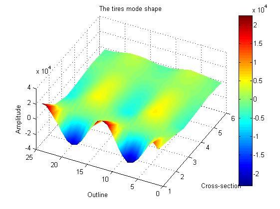
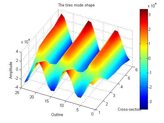
84 Mode 3 Circumference Mode 4 Circumference 78