Steady State And Dynamic Analysis And Optimization Of Single-stage Power Factor Correction Converters

Transcription

1 University of Central Florida Electronic Theses and Dissertations Doctoral Dissertation (Open Access) Steady State And Dynamic Analysis And Optimization Of Single-stage Power Factor Correction Converters 2007 Khalid Rustom University of Central Florida Find similar works at: University of Central Florida Libraries Part of the Electrical and Electronics Commons STARS Citation Rustom, Khalid, "Steady State And Dynamic Analysis And Optimization Of Single-stage Power Factor Correction Converters" (2007). Electronic Theses and Dissertations This Doctoral Dissertation (Open Access) is brought to you for free and open access by STARS. It has been accepted for inclusion in Electronic Theses and Dissertations by an authorized administrator of STARS. For more information, please contact

2 STEADY STATE AND DYNAMIC ANALYSIS AND OPTIMIZATION OF SINGLE-STAGE POWER FACTOR CORRECTION CONVERTERS By KHALID W. RUSTOM B.S. Princess Sumaya University for Technology, 2000 M.S. University of Central Florida, 2002 A dissertation submitted in partial fulfillment of the requirements for the degree of Doctor of Philosophy in the Department of Electrical Engineering and Computer Science in the College of Engineering and Computer Science at the University of Central Florida Orlando, Florida Fall Term 2007 Major Professor: Issa Batarseh

3 2007 Khalid Rustom ii

4 ABSTRACT With the increased interest in applying Power Factor Correction (PFC) to off-line AC-DC converters, the field of integrated, single-stage PFC converter development has attracted wide attention. Considering the tens of millions of low-to-medium power supplies manufactured each year for today s rechargeable equipment, the expected reduction in cost by utilizing advanced technologies is significant. To date, only a few single-stage topologies have made it to the market due to the inherit limitations in this structure. The high voltage and current stresses on the components led to reduced efficiency and an increased failure rate. In addition, the component prices tend to increase with increased electrical and thermal requirements, jeopardizing the overarching goal of price reduction. The absence of dedicated control circuitry for each stage complicates the power balance in these converters, often resulting in an oversized bus capacitance. These factors have impeded widespread acceptance of these new techniques by manufacturers, and as such single stage PFC has remained largely a drawing board concept. This dissertation will present an in-depth study of innovative solutions that address these problems directly, rather than proposing more topologies with the same type of issues. The direct energy transfer concept is analyzed and presented as a promising solution for the majority of the single-stage PFC converter limitations. Three topologies are presented and analyzed iii

5 based on this innovative structure. To complete the picture, the dynamics of a variety of single-stage converters can be analyzed using a proposed switched transformer model. iv

6 To my wife and parents for their love, support, and inspiration v

7 ACKNOWLEDGMENTS I wish to thank all my professors who have contributed to the work presented in this dissertation. In particular, I would like to thank my advisor Dr. Issa Batarseh for our numerous discussions in which he provided the suggestions and the inspiration which made this work possible. In addition, I would like to express my gratitude to Drs. Chris Iannello, Weihong Qiu, and Shiguo Luo for spending many hours helping me. I also wish to thank the other members of my committee, Drs. John Shen, Takis Kasparis and Thomas Wu for serving on my committee and providing helpful comments. Finally, I wish to thank my colleagues C. Jourdan, O. Abdel, and H. Al- Atrash for being there beside me at all times. vi

8 TABLE OF CONTENTS LIST OF FIGURES... XI LIST OF TABLES... XVII CHAPTER 1 INTRODUCTION Introduction Definition of Power Factor and Harmonic Distortion Harmonics Standards and Regulations Classification of Power Factor Correction Approaches Research Motivations Dissertation Outline CHAPTER 2 OVERVIEW OF SINGLE-STAGE POWER FACTOR CORRECTION TECHNIQUES Introduction Original Single-Stage Topologies DC Bus Voltage Feedback CCM Operation of the PFC Cell Direct Energy Processing Approach CHAPTER 3 IMPROVED ASYMMETRIC HALF-BRIDGE SOFT- SWITCHING PFC CONVERTER USING DIRECT ENERGY TRANSFER TECHNIQUES Introduction The Original Asymmetric Half-Bridge Converter The Proposed Soft-Switching Topology vii

9 3.3.1 Principle of Operation Steady-State Analysis Design Curves Design Examples Simulation and Experimental Results Summary CHAPTER 4 ANALYSIS, DESIGN, AND OPTIMIZATION OF THE BI- FLYBACK CONVERTER Introduction Principle of Operation Flyback Operation Mode Boost Operation Mode Steady State Analysis Duty Cycle Intermediate Bus Voltage DCM Condition for the PFC Cell CCM Condition for the DC-DC Cell Design Equations and Methodology Main Equations and Design Curves Stress Equations Design Example Simulation Results Experimental Results Summary viii

10 CHAPTER 5 AVERAGE MODELING AND AC ANALYSIS OF PFC CONVERTERS Introduction The Switched Transformer Model (STM) Principle of Operation The Switched Transformer Model (STM) Operation Modes Unified Model Equations Average Modeling Applied to the Bi-Flyback Converter Experimental Results Summary CHAPTER 6 ANALYSIS, DESIGN, AND OPTIMIZATION OF THE CENTER-TAPPED FLYBACK CONVERTER Introduction Principle of Operation Mode 1 Operation Mode 2 Operation Steady State Analysis Duty Cycle Intermediate Bus Voltage DCM Condition for the Input boost inductor CCM Condition for the DC-DC Cell Design Equations and Methodology Main Equations and Design Curves Stress Equations Design Example Simulation Results ix

11 6.6 Experimental Results Summary CHAPTER 7 SUMMARY AND FUTURE WORK Summary and Conclusions Future Research LIST OF REFERENCES x

12 LIST OF FIGURES Figure 1-1 The European Standard (IEC) Divisions... 7 Figure 1-2 Class D Special Waveform Figure 1-3 General Structures of the Passive PFC Approaches Figure 1-4 Power Waveforms Associated with Resister Emulator PFC Stage Figure 1-5 System Configuration of Two-stage PFC Power Supply Figure 1-6 System Configuration of Single-stage PFC Power Supply Figure 2-1 the BIFRED Converter Figure 2-2 Switching Frequency vs. Load Current Figure 2-3 Single-stage Boost/Flyback Combination Circuit Figure 2-4 Single-stage PFC converter: (a) Boost/Flyback with DC-bus Voltage Feed-back, (b) BIFRED with DC-bus Voltage Feed-back Figure 2-5 Modes of Operations in the DC-bus Voltage Feedback Topologies Figure 2-6 Current Source CCM PFC Circuit Figure 2-7 Effective Duty Cycle in Single-Stage PFC Figure 2-8 Voltage Source CCM PFC Circuit Figure 2-9 Power Relationship in Single-Phase PFC Converters Figure 2-10 Block Diagram for the Direct PFC Scheme Figure 2-11 Parallel Power PFC Converter Figure 2-12 Single-switch PFC Converter with Inherent Load Current Feedback Figure 2-13 Boundary Modes of Operation during Half-line Cycle Figure 2-14 Energy Transfer Paths during the two Modes of Operation Figure 2-15 Power flow Diagram of the Proposed Scheme xi

13 Figure 2-16 Basic Circuit Schematic of the AHBC Converter Proposed in Chapter Figure 3-1 Half-Bridge Forward Converter Figure 3-2 Switching Waveforms: (a) Symmetric witching, (b) Asymmetric switching Figure 3-3 The DC-DC Conversion Characteristics of the Asymmetric converter Figure 3-4 Asymmetric Half Bridge Forward Converter with unbalanced magnetic and current doubler Figure 3-5 M vs. D for the Asymmetric Converter with Unbalanced Magnetics Figure 3-6 Single Capacitor Asymmetric Converter Figure 3-7 Basic circuit schematic of the proposed Asymmetric Converter Figure 3-8 Regions of Operation During one Line Cycle Figure 3-9 Equivalent Topologies for the Three Switching Modes Figure 3-10 Operation Waveforms Figure 3-11 Power Flow over the Line Period Figure 3-12 MathCAD Numerical Solve Block Figure 3-13 M vs. D under different τ n values Figure 3-14 M vs. D under different n 2 values Figure 3-15 M vs. D under different n 1 values Figure 3-16 Storage capacitor voltage of the converter Figure 3-17 Numerical Solution for n1 vs.τ n Figure 3-18 Simulation Waveforms of the Proposed Converter, First trace: Line Voltage, Second trace: Input Current, Third trance: Flyback Current, Fourth trace Output Inductor Current Figure 3-19 Line current (upper trace) and Line voltage (lower trace) Figure 3-20 Efficiency versus Line voltage xii

14 Figure 4-1 BIFRED Topology for Single-stage PFC Applications Figure 4-2 The Bi-flyback Topology Figure 4-3 Modes of Operation during a Line Cycle Figure 4-4 Equivalent Circuits for the Three Intervals during the Flyback Mode Figure 4-5 Key Waveforms during Flyback Mode Operation Figure 4-6 Equivalent Circuits for the Three Intervals during the Boost Mode Figure 4-7 Key Waveforms during Boost Mode Operation Figure 4-8 Power Flow Over a line cycle Figure 4-9 Direct Transferred Power to the Output during Line Cycle Figure 4-10 MathCAD Solve Block Figure 4-11 Bus Capacitor Voltage versus n1 for Different PD Values Figure 4-12 Average Power Percentage Directly Delivered to the Output versus n1 for Different PD Values Figure 4-13 RMS value of the Switch Current versus n1 for Different PD Values Figure 4-14 THD versus n1 for Different PD Values Figure 4-15 PF versus n1 for Different PD Values Figure 4-16 Lm1 versus n1 for Different PD Values Figure 4-17 Lm2 versus n1 for Different PD Values Figure 4-18 n2 versus n1 for Different PD Values Figure 4-19 Simulation Schematics for the Bi-flyback Converter Figure 4-20 Simulation Waveforms during the Flyback Mode Figure 4-21 Simulation Waveforms during the Boost Mode Figure 4-22 Input Current Simulation Waveforms over Switching Cycles xiii

15 Figure 4-23 Measured Efficiency versus Output Power at 110Vrms Figure 4-24 Measured Bus Voltage versus Output Power at 110Vrms Figure 4-25 Measured Efficiency when the Input Voltage Varies between Vrms at Rated Output Power Figure 4-26 Measured Bus Voltage versus Input Voltage at Rated Output Power Figure 4-27 Measured Power Factor versus Input Voltage at Rated Output Power Figure 4-28 Measured Input Current at rated Output Power, 110Vrms Figure 4-29 Measured output voltage (AC coupled) at rated power, 110Vrms Figure 4-30 Measured output voltage (AC coupled) at rated power, 180Vrms Figure 5-1 Switch Models (a) PWM Switch, (b) GSIM Figure 5-2 The Bi-flyback PFC Converter Figure 5-3 The Proposed Five-terminal Switched Transformer Model Figure 5-4 Flyback versus Boost Operation Figure 5-5 Time Duration Definition of the Proposed Model Figure 5-6 Primary and Secondary Current Waveforms in the Flyback and Boost Modes Figure 5-7 Average Model implementation in Pspice Figure 5-8 Operational Modes of the Bi-flyback Converter during One Line Period Figure 5-9 The Bi-flyback PFC Converter Switching and Average Simulation Models Figure 5-10 The Bi-flyback PFC Converter Simulation Results Figure 5-11 Control to Output (V o /d) Frequency Response Simulation Results Bi-Flyback by Average Model xiv

16 Figure 5-12 Experimental Control to Output Voltage (V o /d) Frequency Response measured for the Bi-flyback PFC converter Figure 5-13 Frequency Response Measurement Setup Figure 6-1 The Center-Tapped Flyback Topology Figure 6-2 Modes of Operation during a Line Cycle Figure 6-3 Equivalent Circuits for the Three Intervals during Mode Figure 6-4 Key Waveforms during Mode 1 Operation Figure 6-5 Equivalent Circuits for the Three Intervals during Mode Figure 6-6 Key Waveforms during Mode 2 Operation Figure 6-7 Average Input Current during Line Cycle Figure 6-8 Average Flyback Magnetizing Current during Line Cycle Figure 6-9 MathCAD Solve Block Figure 6-10 THD versus Np for Different N Values Figure 6-11 PF versus Np for Different n Values Figure 6-12 Direct Energy Transferred to the Output over Half Line Cycle 181 Figure 6-13 Direct Energy Transferred to the Output versus Np for Different n Values Figure 6-14 Main Switch Conduction Losses versus Np for Different n Values Figure 6-15 Lin Energy versus Np for Different n Values Figure 6-16 Lm Energy versus Np for Different n Values Figure 6-17 Zoomed-in from Figure Figure 6-18 Maximum Switch Current during a Line Cycle Figure 6-19 MOSFET and Diode Voltage Stress versus Np Figure 6-20 MOSFET Peak Current Stress versus Np for Different n Values xv

17 Figure 6-21 MOSFET Estimated Switching Losses versus Np for Different n Values Figure 6-22 Circuit Schematics of the Simulated Center-tapped Flyback Converter Figure 6-23 Simulation Waveforms during Mode 1 Operation Figure 6-24 Simulation Waveforms during Mode 2 Operation Figure 6-25 Simulation Waveforms during Line Cycle Figure 6-26 Simulation Result for the filtered Input Current Waveform Figure 6-27 Measured Efficiency versus Output Power for 110Vrms and 220Vrms Input Voltages Figure 6-28 Measured Efficiency when the Input Voltage Varies between Vrms at Rated Output Power Figure 6-29 Measured Bus Voltage versus Output Power for 110Vrms and 220Vrms Input Voltages Figure 6-30 Measured Bus Voltage when the Input Voltage Varies between Vrms at Rated Output Power Figure 6-31 Measured Power Factor when the Input Voltage Varies between Vrms at Rated Output Power Figure 6-32 Input Current Waveform at 110Vrms under Full Load Figure 6-33 Input Current Waveform at 220Vrms under Full Load xvi

18 LIST OF TABLES Table 1-1 Harmonic Emission Limits for IEC and IEC Table 1-2 Relative Performance Comparison of Three PFC Approaches Table 3-1 Switching Modes: time intervals and status of devices Table 4-1: Bi-flyback Design Specifications Table 4-2: Bi-flyback Design Example Calculation Results Table 4-3: Prototype Measurement Results for 110Vrms Input Voltage Table 4-4: Prototype Measurement Results when the Input Voltage is changed from Vrms Table 5-1 Converter Specification and Performance Table 6-1: Center-tapped flyback Converter Design Specifications Table 6-2: Summary of Design Results Table 6-3: Experimental Testing Data at 110Vrms Table 6-4: Experimental Testing Data at 110Vrms Table 6-5: Experimental Testing Data between Vrms xvii

19 CHAPTER 1 INTRODUCTION 1.1 Introduction In recent years, new regulations have fostered interest in Power Factor Correction (PFC) techniques. The demand for PFC has been increasing for today s off-line power supplies and even those at low power levels. The offline AC-DC power converters employed in most of today s electrical equipment have been a significant source of harmonic distortion drawing distorted current waveforms, polluting the mains, and thereby degrading power quality. Today, a manufactured converter should satisfy acceptable power quality metrics. Power quality issues have always been a significant topic in power engineering, but, in recent years, this topic has drawn a special attention due to the increased use of high performance electronic devices [1, 2]. The majority of the Modern PFC converters either utilize a simple and economical passive filtering technique (low power), which cannot meet the full range of power quality requirements, or use an additional front-end converter for the PFC function (resulting in a two stage approach). With the help of advanced research in this field, a new approach attracted more attention, namely the integrated single-stage converters. By integrating the two-stage converter into a single-stage, which performs both the PFC and DC-DC conversion simultaneously, this new field promises regulation 1

20 compliant converters that cost less, are more reliable by using fewer components, and employ a simpler structure. The research proposed for this dissertation is intended to assist the development of new, advanced AC-DC power converters with PFC to be used mainly in low power applications. Referring to the standards and regulations on harmonic emission, these converters are classified as Power Factor Correction (PFC) AC-DC converters. In this Chapter, the definition of power factor and harmonic distortion will be reviewed, followed by a summary of the effects of power electronics pollution. After which, the new power quality regulations will be summarized. In addition, the motivation and research objectives will be introduced at the end of this chapter. 1.1 Definition of Power Factor and Harmonic Distortion During the transmission and distribution of electrical power, the utility voltage waveform maybe distorted by a number of factors, some of which occur within the customer s own installations. This waveform distortion, when steady state and periodic, is a result of harmonic and means the voltage waveform is no longer a perfect sinusoid. In the development that follows, this distortion will be expressed mathematically. If we assume a periodic waveform, f(t), then the Fourier series expansion representation for this waveform will be [3], 2

21 f () t = F + f () t + f () t f ( t) n n= 1 n = F + ( a cosnωt + b sin nω t) (1.1) n where, F0 represents the average (DC) value of f(t), n represent the order of the harmonic and the coefficient an and bn are evaluated from the following integrals, T 2 an = f ( t)cos nω tdt n = 1,2,3,..., (1.2) T 0 T 2 bn = f ( t)sin nω tdt n = 1,2,3,..., (1.3) T 0 where T is the period of the waveform and equal to 2π/ω. The definition of the power factor is the ratio of the real power (average) to the apparent power, as described in Eq. (1.4). PowerFactor ( PF) = Real Power( Average) (1.4) Apparent Power In practice, power electronics systems have nonlinear behavior due to switching devices. Applying the definition of power factor to a distorted current and voltage we can express the power factor as, 3

22 PF = 1 T T 0 1 T T 0 v( t) 2 v( t) i( t) dt dt 1 T T 0 i( t) 2 dt = n= 1 I sn, rms I V s, rms sn, rms V s, rms cos θ n (1.5) where, Vsn,rms and Isn,rms are the rms values of the n th harmonic voltage and current, respectively, and θn is the phase shift between the n th harmonic voltage and n th harmonic current. For off-line power supplies where the input voltage is almost a purely sinusoidal, Eq. (1.5) can be further simplified to, PF I s1, rms = 1 I s, rms cos θ = k d k θ (1.6) where, I s1,rms : rms value of the fundamental component in line current; kd = Is1,rms/Is,rms: distortion factor; k θ = cosθ 1 : displacement factor. Another important term that is used to measure the quality of the waveform is the Total Harmonic Distortion (THD). Again assuming the typical nearly sinusoidal voltage input, the input current THD, is defined as: 4

23 THD i = n = 2 I I 2 sn, rms 2 s1, rms = k d (1.7) There are many negative effects caused by the existence of the harmonic content. This distortion has several detrimental effects, including but not limited to the following: Heat and losses: the current harmonics cause an increase in the copper losses (conduction), and the voltage harmonics result in an increase in iron losses (core magnetic). Inefficient power utilization: the current harmonics increase the rms value of the total current but they do not deliver any real power in Watts to the load, resulting in inefficient use of capacity and unnecessary over rating of the distribution. Protection failure and safety risks: Fuses and relays can also be affected in the present of harmonics and they may cause nuisance tripping. Changing the network impedance: all the network components present complex impedances that will vary when presented with the harmonic frequencies. Exhausting the power cables: harmonics will lead to the increase in the ac resistance of a cable is caused by two phenomena, skin 5

24 effect and proximity effect. This can result in increasing the losses and may cause insulation failure in the cable. Electro-Magnetic Interference (EMI) Problems: The high frequency disturbances often categorized as EMI can be radiated to free space as electromagnetic waves or conducted though the power lines in a differential or common mode. EMI s effect on electronic systems is commonly the subject of power engineer s study. In order to maintain harmonic distortion at reasonable levels and to comply with the regulatory standards on distortion there are solutions which are applicable to both the supply system and to the harmonics sources themselves. These solutions will be presented thoroughly in the next chapter. 1.2 Harmonics Standards and Regulations The added circuitry to improve the power factor and overcome the harmonics problem will add extra cost to the original power supply, typically 20 to 30 percent more cost. This extra cost has made the power supply manufacturers less interested in implementing these circuits. On the other hand, the power company wants its consumers to draw clean current waveforms from its mains. Thus international and national standards have 6

25 come into force to limit the level of harmonic injection into the system and to maintain good power quality [4, 5]. Figure 1-1 The European Standard (IEC) Divisions The IEEE-Std-519: 1992, recognized as recommended practice in the U.S., is mainly used in the American market for guidance in the design of power systems with non-linear loads. This standard contains, in a single publication, all the topics related to the analysis and control of harmonics in the power system. On the other hand, the European standard (International Electro-technical Commission) IEC presents standards on electromagnetic compatibility in several publications that cover many disturbance phenomena: harmonics, inter-harmonics, voltage fluctuations, voltage imbalance, mains signaling, power frequency variation and DC components. Figure 1-1 shows the divisions of the European standards that superseded the old IEC 555-2/EN These divisions depend on the load, 7

26 equipments connections, and whether it is low, medium, or high voltage and it also depends on the maximum current drawn per phase by the equipment. Table 1-1 Harmonic Emission Limits for IEC and IEC Harmonic Number (n) Class A Limits ** Class B Limits ** Class C Limits * (A rms ) (A rms ) % Of fundamental Class D IEC Limits * limits for TV(>165W) ma/w of input power (50-600W) (A rms ) Max DC current<0.05a n/a x PF n/a n/a n/a n/a n/a n/a n/a n/a n/a n/a n/a n/a n/a n/a Even /n 2.760/n n/a n/a n/a Odd /n 3.338/n /n 1.5/n * EC only ** Both IEC and IEC The IEC sets limits for the harmonic currents generated by electrical and electronic equipment drawing input current up to 16A/phase. The standard categorizes the equipment into four classes: Class B for portable tools. Class C for lighting equipment including dimmers. 8

27 Class D for equipments having the special waveform, shown in Figure 1-2, of input current and an active input power less than or equal to 600W, except phase angle controlled motor driven equipment. Class A for everything else and balanced three-phase equipment. Table 1-1 shows the harmonic limits for these classes. An envelope, shown in Figure 1-2, defines the special wave-shape for Class D. Equipment is deemed to be Class D if the input current waveform for each half period is within the envelope for at least 95% of the duration of its half cycle. The centerline of the envelope coincides with the peak of the input current, which may be not the same position of the peak line voltage. The envelope is divided into three equal periods of π/3 with the amplitude of the center period is equal to the peak of the input current and the amplitude of the two sides is equal to 0.35 of that peak value. If the input current is approximately a sinusoid it will fall outside of that envelope for 40% of the cycle. Note that if the power above 600W, it is not a Class D product and hence should be tested for Class A limits. If the power is below 75W, no limits apply. 9

28 π/3 π/3 π/3 i pk i in 0.35 i pk π/2 π/2 v in Figure 1-2 Class D Special Waveform 1.3 Classification of Power Factor Correction Approaches The general approaches to improve power factor can be widely classified as passive and active approaches. The passive approaches uses capacitive inductive filters to achieve PFC, while the active approaches use a switched- Mode power supply to shape the input current. In this section both approaches will be discussed and some of the common circuits will be presented. A. Passive Approaches In this approach, a full bridge rectifier with an LC filter is used to meet the line current harmonic limits. Generally, the LC filter can be placed on the AC-side or the DC-side of the rectifier as shown in Figure 1-3. Placing the LC filter on the ac-side will result in purely sinusoidal input current. 10

29 v ac Passive Passive + DC- DC _ PFC PFC Conveter Filter Filter L O A D or CONTROL + _ + _ Figure 1-3 General Structures of the Passive PFC Approaches Passive PFC can meet the regulation with high efficiency, superior reliability, low cost, and low EMI. On the other hand, the filter capacitor voltage varies with the line voltage, which has a detrimental effect on the performance and efficiency of the DC-DC converter. When considering the hold-up time for the power supply, the capacitance of the bulk capacitor has to be increased and become very bulky compared to what it would have been without this varying voltage. As a result of this trade, the passive approaches seem to be more attractive in low power applications, up to 300Watts. This lack of voltage regulation and poor dynamic response make passive PFC more suitable for applications with a narrow line voltage range. Other drawbacks are the size and weight of the filter choke inductor. This inductor is heavy, bulky, and requires careful design consideration. Even with these limiting factors, the majority of power supplies manufactured in low power and cost sensitive applications have adopted this passive technique. 11

30 B. Active Approaches In active PFC, a switched-mode converter is employed to overcome the limitations of the passive approaches. As seen in Figure 1-4, the ideal result from this PFC stage, is to achieve a unity power factor. Assuming unity power factor, the line current should be sinusoidal and in phase with the line voltage. That will result in pulsating output power than contains in addition to the real (average power), an alternating component with double the line frequency. Since the power demanded by most loads is constant, an energy storage element is needed. Since the inductor-stored energy cannot supply this amount of energy, another storage component is needed. The storage capacitor, C S, which will handle the double line frequency ripple component, is introduced. This capacitor is usually large and bulky. i ac v ac + _ C s L O A D v ac p in (t) DC- DC Conveter that works as resistor emulator p o1 (t) p o2 (t) P in P o1 P o2 Figure 1-4 Power Waveforms Associated with Resister Emulator PFC Stage 12

31 The double line frequency problem that presents itself on the output of the PFC stage cannot be internally solved. Usually a compromise between PFC and output voltage ripple can be made, but most of the time this output voltage is not good enough to supply the load. As a result, another DC-DC converter, or the so called post regulator, is required to solved this problem and achieve tight output regulation. The result is the most flexible PFC configuration that is called the active, two-stage PFC, shown in Figure 1-5. v ac + _ PFC Converter C s DC- DC Conveter L O A D CONTROL CONTROL Figure 1-5 System Configuration of Two-stage PFC Power Supply The boost converter is widely used in the PFC stage due to its advantages such as good power factor, grounded switch, input inductor and simplicity. Usually this PFC converter has a low bandwidth control which implies a loosely regulated output voltage across the storage capacitor. In universal line voltage applications, the DC bus voltage may vary between V. Because of the relative high voltage on the storage capacitor, the 13

32 value of the capacitance can be optimized to provide the necessary hold-up time. The DC-DC converter is connected to the storage capacitor to provide the necessary output voltage regulation with the appropriate gain and often provides isolation. Another family under the active approach is the single-stage configuration. This configuration was introduced as a way to reduce the cost and complexity of the two-stage structure [6]. In reality, it can be viewed more as a modification of the conventional two-stage PFC rather than as a class by itself. As can be seen in Figure 1-6, the PFC and the DC-DC cell share the control circuit and may also share the switches in this configuration. The energy storage capacitor between the two stages serves as a buffer and to provide the converter with the necessary hold up time. However, in the single-stage configuration, the voltage across the storage capacitor is not regulated, because the controller is used to regulate the output voltage. As a result this voltage can vary greatly, usually between V in universal line applications, depending on the topology. This will have a negative impact on the design and cost of the PFC converter as will be discussed in the following Chapters. 14

33 v ac + _ PFC Cell DC- DC Cell L O A D CONTROL Figure 1-6 System Configuration of Single-stage PFC Power Supply C. Approach Comparisons Generally, in low power applications and especially when designing to meet the minimum regulation requirements, if line voltage can be considered fairly invariant, the passive approach should be considered. However, a major drawback of the passive approach is the size and weight of the filtering components. On the other hand, when unity power factor is required, or when size is a key objective, or if the application requires high power, the active PFC is the only practical solution. At low power levels, the active single-stage offers a great advantage over the passive approaches due to its simple structure, low cost, minimum weight and better PFC performance, even still, its performance, size, and cost are questionable when it compared to the two-stage approach. The following are the major problems associated with the single-stage active PFC approach: Intermediate Bus Voltage and Power Balance Issue: As mentioned before, the single-stage converter has only one 15

34 feedback control circuit to tightly regulate the output voltage. As a result, the intermediate bus voltage is kept unregulated and its voltage level depends on PFC cell topology. Since most likely the boost topology will be selected, this voltage may reach values of 1000V in a typical design depending on the line and load condition due to power balance requirements. To illustrate this condition, assuming that the DC-DC cell operates in CCM for enhanced performance, then the duty cycle will not change with load changes. When the load demand decreases, the input power will not change and all the power difference will be stored in the intermediate bus, raising its voltage to high levels. This condition will continue until a new power balance condition is achieved, since with the increase in the bus voltage, the duty cycle will be reduced to keep the output voltage regulated. More about the high intermediate bus voltage can be found in [7]. Since the intermediate bus capacitor should be selected to handle a high voltage rating, this will increase the converter cost considerably since capacitors with voltage ratings higher than 450V are uncommon. The MOSFET voltage rating will also be increased affecting its losses and price as well. High current ratings: One way to get around the increased bus voltage is to use DCM operation for the DC-DC cell. In DCM, the 16

35 duty cycle depends on the load condition and hence the bus voltage will not increase is the same manner as in the previous case. On the other hand, the DCM operation comes with its own set of disadvantages. In particular, a requirement for higher peak current ratings for the components in the DCM converter resulting in device selection with higher cost and lower efficiency. Sometimes a selector switch ( V) will limit some of these problems, but generally, a trade-off between improving the size and cost using single switch and one controller, to the cost and size of the storage capacitor should always be considered. In addition, a more expensive EMI filter in needed when operating the PFC cell in DCM to achieve automatic current shaping. Unity power factor and tight output regulation for any power range can be achieved using the two-stage, active PFC. This structure is fully capable of compliance with regulations and is compatible with universal line voltage applications. Some negative factors include the increased cost and size associated with the two staged approach and sometimes the reduced efficiency associated with processing the power through two stages versus one. In specific applications, all of the three options are capable of regulation compliances. Table 2-1 provides a general relative performance comparison 17

36 for the passive and active single and two-stage approaches with the current available technologies [8]. Table 1-2 Relative Performance Comparison of Three PFC Approaches Performance Review Passive Scheme Active Two-stage Active Single- Stage THD High Low Medium Power Factor Low High Medium Efficiency High High medium Size Large Medium Medium-Small Bulk Cap Voltage Variation Constant Variation Control Simple Complex Medium Component Count Least Medium Medium-Low Power Range < 300 W Any < 300 W Design Difficulty Low Medium High 1.4 Research Motivations In this section, the motivations behind this work are outlined. The existing PFC techniques, utilized in the marketplace today, are either a two stage structure that provides a unity power factor with high efficiency, or using passive components that cannot meet the regulation requirements. While the first solution has flexible structure that can lead to superior performance, it exceeds regulatory requirements on harmonic content while adding a 30% increase in the component count, and increasing the cost and the size of the converter. No other solution can compete with the 18

37 performance of the two stage approach, but at the same time, this performance is not required to meet the regulations and it comes with a higher price tag. All the previous attempts to integrate the two stage converter in to a single-stage were not completely successful due to several factors. First, the uncontrolled bus voltage was high, demanding an expensive capacitor. Second, high voltage and current stresses inherent in the design resulted in over-sized, expensive components and low conversion efficiency. Finally, in order to overcome these drawbacks, complex single-stage structures were proposed that have even more components than the two stage converters. Clearly these proposed schemes missed the underlying attraction to single stage PFC potential cost reduction. Much literature has been devoted to single-stage converters with a direct energy transfer technique to solve the limitation of the single-stage approach. None of these papers quantified the amount of direct energy transferred to the output. In addition, due to the operation and topology complexity, no clear design curve or trade-off analyses were performed to make it easier for the practicing engineer to develop these topologies into an economically viable product. Based on these motivations the objectives of this dissertation are: 19

38 To review and investigate various recent techniques in harmonic reduction and power factor correction related to the single-stage structure, and in particular, to topologies with a direct energy transfer mechanism. To develop cost and performance justified topologies that adopt these improving techniques To perform a comprehensive analyses of these converters, and produce the design procedure and curves need for development. To compare the performance and draw conclusion for future research 1.5 Dissertation Outline Chapter 2 will include a comprehensive review of single-stage power factor schemes and highlight some recent techniques that can be adapted to improve performance. In Chapter 3, the improved asymmetric half bridge converter with a parallel energy transfer branch will be introduced and analyzed. Chapter 4 will introduce the bi-flyback topology as a candidate topology to compete with current state of art converters. Operation, topology analysis, and design curves will be provided and the key relationships will be derived. Chapter 5 will focus on the average modeling. A new five-terminal general average model will be defined and its terminal relations will be derived. The new model will be used to obtain the frequency response of the 20

39 proposed bi-flyback converter. In Chapter VI, the center-tapped flyback converter will be proposed to overcome some of the limitations of the biflyback topology. Chapter VII will summarize the results obtained in this dissertation and propose some future work. 21

40 CHAPTER 2 OVERVIEW OF SINGLE-STAGE POWER FACTOR CORRECTION TECHNIQUES 2.1 Introduction This chapter presents an overview of various topological implementations of the single-stage power factor correction converter [9] that has been recently published in the open literature. The discussion in this chapter includes commonly used strategies and various types of converter topologies. A comparison between these strategies and converter topologies will be given. Since object of the work is to improve mainly the efficiency and reduce the stress on the PFC converters while keeping cost competitive, only relevant topologies are discussed. While the literature is rich with publications on this topic, only few address a truly feasible solution. The direct energy transfer capability of these topologies is considered a major improvement technique offering a promising efficiency advantage. This approach will be used in the topologies proposed in later Chapters. 2.2 Original Single-Stage Topologies One of the earliest converters proposed to alleviate the component count, cost, and complexity issues of the two-stage approach was the BIFRED converter [6]. The BIFRED is an integrated boost-flyback converter using a single-switch and a single-controller to achieve both high input PFC and tight output voltage regulation simultaneously, as shown in Figure 2-1. The main 22

41 advantage of this structure lies in the fact that the transformer primary side is in series with the bus capacitor. As a result, the capacitor voltage is reduced by the amount of the reflected output voltage. The converter s proposed operation was DCM for the input boost inductor and CCM for the flyback output DC-DC converter. This is done in order to achieve both automatic PFC at the input and to reduce RMS current at the output. The main disadvantage of this topology is the high storage capacitor voltage due to the power imbalance. This voltage can be as high as 1000V at light load conditions, and this solution becomes impractical when considering the commercial 450V capacitors and 600V MOSFETS. Figure 2-1 the BIFRED Converter To alleviate the stress on the bus capacitor, variable frequency operation was proposed in [10]. In this contribution, it was noted that the DC-DC converter gain depends only on the duty cycle, while the input PFC circuit gain depends on the frequency but not duty cycle, as shown in Eq. (2.1). 23

42 V cs V in = n V Lf I 2 o s o nvo (2.1) As a result, increasing the switching frequency at lighter load can regulate the bus capacitor voltage. While this method can effectively regulate the bus voltage, the implementation faces many difficulties due to the required frequency variation. These difficulties include the following: The frequency has to vary up to 10 times to maintain the bus voltage at 450V as the load decreases to 10%, as shown in Figure 2-2. This high switching frequency will lead to efficiency degradation due to switching losses. Complex magnetic design including the main transformer and the filter. 24

43 - Fs(kHz) Vcs=450V Vcs=600V Vcs=900V Io(A) Figure 2-2 Switching Frequency vs. Load Current In order to overcome the limitation in the DCM-CCM operation, a family of Single-Stage Isolated Power-factor-correction Power supply (SSIPP) was proposed in [11, 12], shown in Figure 2-3. The basic principle of operation is that both the PFC and the DC-DC cells always operate in DCM to alleviate the power balance issue. While the proposed method was effective in reducing the bus voltage, it was not possible to use the 450V capacitor because the voltage is still higher than 500V under high line voltage. In addition, the proposed DCM operation for the DC-DC stage will result in high peak current on the secondary side of the transformer, which will have the added consequence of reduced efficiency due to conduction losses. The high ripple current in the secondary side will also lead to an increase in filter size at the output. 25

44 Figure 2-3 Single-stage Boost/Flyback Combination Circuit 2.3 DC Bus Voltage Feedback One of the most effective techniques to solve the excessive DC bus voltage is called DC bus voltage feedback [13-18]. In this technique a coupled inductor to the DC-DC transformer is added in the charging path on the boost inductor, as shown in Figure 2-4. By inspection, this coupled inductor will act as a negative feedback branch that feeds scaled bus voltage to the charging path of boost inductor and steady state balance can keep the bus voltage below 450V, while the DC-DC converter is operating in CCM. 26

45 (a) D 1 V in n 3 D 2 L C o V o S C s n 1 :n 2 + (b) Figure 2-4 Single-stage PFC converter: (a) Boost/Flyback with DC-bus Voltage Feed-back, (b) BIFRED with DC-bus Voltage Feed-back In addition to the reduced bus voltage stress, this topology can reduce the current stress on the main switch. This is as a result of the aid given by the introduced winding in charging the magnetizing inductor of the DC-DC transformer. This leads to less current discharged from the bus capacitor and less current processed by the switch. This topology also includes a direct energy transfer period since the discharging current from the boost inductor 27

46 will be coupled directly to the output without the need to be processed twice. The same technique is used in the proposed converter in Chapter 6. On the other hand, the operation of this topology includes a Mode that does not allow the full conduction angle of the input line current as shown in Figure 2-5. Mode 1 happens when the reflected bus voltage is higher than the rectified input voltage and depends on the amount of the bus voltage feedback (n 2 /n 1 ratio). The limited conduction angle will deteriorate the Power Factor (PF) performance of the converter and increase distortion. In order to comply with the regulations, the amount of voltage feedback has to be limited, and as a result the reduced switch losses and the amount of direct energy transfer have to be limited as well. This tradeoff between performance and PF results in low efficiency, approximately 71% as reported in [17]. This type of feedback is indirect because the feedback occurs after the bulk capacitor voltage increases. In conclusion, while this topology can limit the bus voltage to a reasonable value, the PF and THD requirements limit the direct energy transferred and the amount of efficiency improvements that can be expected with the voltage feedback feature. 28

47 Figure 2-5 Modes of Operations in the DC-bus Voltage Feedback Topologies 2.4 CCM Operation of the PFC Cell To enhance the efficiency in higher power applications, CCM operation of the single-stage PFC converter was proposed in [18-20]. While CCM operation is usually employed in the two-stage approach, a dedicated controller is necessary to modulate the duty cycle in the PFC stage. Enlarging the boost inductor size to force CCM operation in the single-stage approach will only result in high current distortion. This is a result of the fact that the constant duty cycle condition for PFC is only valid during DCM operation. As a result, a new modulation scheme is necessary to modulate the effective duty cycle across the boost inductor, while the actual duty cycle stays constant. To accomplish this task, the topology in Figure 2-6 was proposed in [18, 19]. The principle of operation for this circuit is based on changing the 29

48 effective duty cycle on the boost inductor without changing the actual duty cycle of the converter. The needed effective duty cycle is given by[20], d pfc Vin 1 Sin( ωt) V Cs (2.2) According to this equation, the duty cycle has to change inversely with the line voltage. The circuit in Figure 2-6 accomplishes this task by adding an inductor in the charging path. As shown in Figure 2-7, the added inductor will prevent the main boost inductor from charging up until the currents in both inductors are the same. This action will modify the effective duty cycle to be D on -D off1. At the same time, D off1 depends on the line voltage. When the line voltage increases, the discharge rate will decrease leading to a longer discharge time and reduced effective duty cycle. The same concept can be applied by employing a capacitor in changing path as shown in Figure 2-8. Figure 2-6 Current Source CCM PFC Circuit 30

49 Figure 2-7 Effective Duty Cycle in Single-Stage PFC Figure 2-8 Voltage Source CCM PFC Circuit While the proposed CCM operation might offer a reduction in the size of the EMI filter and reduced current ripple in the bus capacitor, the following should be noted when evaluating this solution: 31

50 CCM operation might offer enhanced efficiency for medium and high power applications. However, the reverse recovery losses of the boost diode present a serious threat in low power applications, where the single-stage approach is especially attractive. The exact equation that describes the unity power factor condition requires a time varying inductance, and as a result, these topologies cannot claim unity power factor operation. The PFC condition previously discussed only applies to CCM operation. While the converter will be designed for CCM operation, it will enter DCM operation each switching cycle at low line voltage. This behavior will create similar effects to the reduced conduction angle in voltage feedback topologies discussed earlier. This topology has a higher RMS current through the single switch when compared to 2 stage topologies. This will result in efficiency reduction. 2.5 Direct Energy Processing Approach Single-stage and two-stage approaches adapt the simple cascade configuration, where two converters are separated by an energy decoupling element, the bus capacitor. To understand the nature of energy transfer and the real need for the decoupling element, the instantaneous input power and 32

51 the average output power waveforms in a single-phase, PFC converter are shown in Figure 2-9. Figure 2-9 Power Relationship in Single-Phase PFC Converters The input power is a square sin function with double the line frequency, p () t = V I sin ωt = 2P sin ωt (2.3) 2 2 in in in o As we can see, the converter has to process a peak power that is twice the output power. At the same time this power has to be stored and then delivered to the output. Typically, the output capacitor is not the correct choice to store this energy for two reasons. First, the output voltage will fluctuate with double line frequency because tight output voltage regulation will require a small output capacitor. The second reason is the required hold- 33

52 up time of the converter. As a result an energy decoupling capacitor is needed in the circuit. The location of the energy storage element becomes critical and general configuration of the topology will play an important role. If we analyze the power waveforms in Figure 2-9, solving for the time when the instantaneous input power is equal to the output power, then integrating the input power to find the relationship between P1 and P2, we can find that 68% of the energy can be transferred directly to the output, and only 32% of the energy has to be stored and then reprocessed to the output. If P1 energy is directly transferred to the output, the output voltage ripple will not see the double frequency, primarily a result of excesses in power storage. As a result of these findings, a new family of converters adapted the direct energy transfer scheme or parallel energy transfer scheme. The main focus is now changed to the topology structure that can accomplish this task with a minimum number of components while delivering maximum energy directly to the output for enhanced efficiency. Figure 2-10 shows the block diagram that illustrates this direct PFC scheme. 34

53 Figure 2-10 Block Diagram for the Direct PFC Scheme Many circuit implementations have been suggested to implement the direct energy transfer scheme[21-27]. Earlier publications were directed more toward two-stage implementation to improve the efficiency [21, 26]. An example of the two stage implementation is shown in Figure While the direct energy transfer mechanism is clear in this topology, the implementation scheme itself involves many components and might not be a good practical implementation. 35

54 Figure 2-11 Parallel Power PFC Converter The direct energy transfer scheme was later adapted in the singlestage implementation. An example of the single-stage implementation is the topology shown in Figure 2-12 [28], which features the direct energy transfer mechanism. This topology utilizes an extra winding on the main flyback transformer to create a voltage course in series with the storage capacitor. Depending on the value of this voltage, the converter will have a limited conduction angle as shown in Figure Before the converter starts to draw current from the input, all the power will be processed from the storage capacitor, as shown in Figure 2-14 (a). After the input voltage reaches a predetermined value, the energy will be processed from the input to the output directly through the flyback converter, and the remainder of the needed energy will be processed from the storage capacitor, as shown in 36

55 Figure 2-14 (b). At the same time, the input inductor will be charging the storage capacitor. While the input voltage continues to increase, more energy will be processed from the input to the output and to the storage capacitor. Near the peak input voltage, the input inductor will change operation from DCM to CCM as a direct result of the increased current processed through the input. Switching between DCM and CCM leads to more line distortion and control difficulties. And as in the majority of the published papers, there was no clear design procedure nor quantified trade-offs between direct energy transfer, PF, and bus voltage. Figure 2-12 Single-switch PFC Converter with Inherent Load Current Feedback 37

56 v in i in n 1 /(n 1 +n 2 ) V cs α t t Figure 2-13 Boundary Modes of Operation during Half-line Cycle (a) 38

57 V in L Charge D 1 n 1 :n 3 D 3 D 2 Discharge n 2 Charge Discharge L ccm C o V o C s + S (b) Figure 2-14 Energy Transfer Paths during the two Modes of Operation A simple implementation scheme was proposed in [29] through the flyboost cell. The mechanism of operation in this scheme relies on introducing a threshold power level P th, as shown in Figure 2-15, and when the input power is lower than this threshold value the power will be transferred directly to the output, portion P 1, otherwise it will be processed twice by both stages, portion P 2. 39

58 p in (t) P o P th P 1 P 2 Figure 2-15 Power flow Diagram of the Proposed Scheme The flyboost cell can be implemented in any boost-based PFC converter, by adding another winding to boost inductor and feed it to the output capacitor [30, 31] as shown in Figure Unlike the previous implementation, the flyboost implementation is simple [32, 33] and can be adapted in many single-stage converters. In general, to implement the parallel energy path for any boost-based PFC converter, we can add another winding to boost inductor and feed it to the output capacitor. On the other hand, the power flow analysis of these converters is more complicated and requires several measures in the design procedure as described in the proceeding chapters. 40

59 L SF D SF T1 n 1 :1 n 2 :1 v AC + V in - L PF D PF C s S 1 D o1 L S1 L oco R o + V o - S 2 L P -V a + L S2 C a T2 D o2 Figure 2-16 Basic Circuit Schematic of the AHBC Converter Proposed in Chapter 3 41

60 CHAPTER 3 IMPROVED ASYMMETRIC HALF-BRIDGE SOFT-SWITCHING PFC CONVERTER USING DIRECT ENERGY TRANSFER TECHNIQUES 3.1 Introduction Of course, the ideal PWM converter is lossless. In reality, power dissipation is due to the non-idealities in the power components and mainly the semiconductor switches themselves. With the improvements in semiconductor technologies, switch performance has become more reliable and the switching losses have been considerably reduced. With these improvements, the converter can be operated at a higher switching frequency, resulting in reduce size and weight of passive components. Switching losses had become the main concern with the current trend of increasing the switching frequency. For certain applications, resonant converters were a promising solution. Resonant converters eliminate nearly all the switching losses and leave the path open for an even higher switching frequency, but still, they too have their drawbacks. During the resonant process, the switch current or voltage reach high values, higher than those in the regular PWM converters, this drawback increases the conduction losses. The Asymmetric Half Bridge Converter (AHBC) provides a good method for soft switching. In this chapter, the development of the original Asymmetric Half Bridge Converter (AHBC) will be presented. In addition, the new, improved AHBC will also be discussed including with a discussion of

61 the detailed analysis and design considerations followed by simulation and experimental results. 3.2 The Original Asymmetric Half-Bridge Converter Soft switching can be achieved in any transformer-coupled PWM converter with half or full bridge configuration operating at 50% duty cycle. By allowing a small, controlled dead time between the two conduction periods, the leakage inductance of the transformer can resonate with the parasitic capacitors in the switches and soft switching can be achieved. The original half bridge forward converter is shown in Figure 3-1[34]. In addition to the potential soft switching, the half bridge configuration allows more power handling capabilities than the single switch topology, and has fewer components than the full bridge configuration making it a good choice for medium power applications. The dead time between the switches can be noticed in Figure 3-2(a). Soft switching can be achieved only at 50% duty ratio. Soft switching will be lost if the converter operates at any other duty ratio because the voltage across the switch will rise back again before the turn ON time of that switch. As a result, no output regulation can be achieved. 43

62 Figure 3-1 Half-Bridge Forward Converter In Figure 3-2(b) we can see how the asymmetric switching scheme can alleviate that problem by operating each switch at a different duty cycle. By using asymmetric switching with a small dead time between switching to achieve lossless switching, we can effectively regulate the output by changing the duty cycle of the switches. Beyond the complementary duty ratio, the main difference between the symmetric and asymmetric switching is the different voltage levels on the upper and lower bridge capacitors, C1 and C2 in Figure 3-1. To find the voltage of each capacitor we can write the input voltage loop equation, Eq. (3.1), and the volt-second balance equation on the primary magnetizing inductor LM, Eq. (3.2). Note that Eq. (3.2) ignores the leakage inductor s effect. V = V C1 + VC 2 in (3.1) VC1 D + VC 2(1 D) = 0 (3.2) 44

63 By solving Eq. (3.1) and Eq. (3.2) we find, V 1 = V (1 D) C in (3.3) V C = 2 V in D (3.4) Using the volt-second balance equation on the output inductor Lo, we can find the gain equation of the asymmetric half bridge converter as, M V = V o 2D( D) = n in 1 (3.5) S1 D S1 D S2 D t S2 1-D t V in /2 t V C1 t v p v p -V in /2 t -V C2 t v s v s V o V o t t (a) (b) Figure 3-2 Switching Waveforms: (a) Symmetric witching, (b) Asymmetric switching 45

64 The plot of the quadratic relationship in Eq. (3.5) is shown in Figure 3-3. The gain is at maximum at a duty ratio of 50% and reaches zero at zero or 100% duty ratio. It is therefore possible to regulate the output voltage by varying the duty ratio while, at the same time, maintain soft switching. 1 n=0.5 M 0.5 n= D Figure 3-3 The DC-DC Conversion Characteristics of the Asymmetric converter The above analysis shows that the AHBC is advantageous in terms of the high operating frequency and soft switching, which allow a simple and small output filter. On the other hand, due to the complementary control mechanism, the switches experience very different levels of stress. Due to the nature of the conversion characteristics shown in Figure 3-3, the converter s duty ratio should be chosen far from the ideal 50% to allow regulation to take place. When the duty cycle is small, one switch suffers very high stress, which deteriorates the performance. To solve this problem, the 46

65 unbalanced magnetic was introduced to bring the duty cycle back closer to the 50%. Figure 3-4 shows the implementation of this solution with a current doubler at the output side [35]. Another realization of the AHBC in the PFC converter can be found in [36] where coupled input inductors were used. n 1 :1 V in + _ S 1 D + C o1 1 C o R o V o - S 2 C 2 D o2 n 2 :1 Figure 3-4 Asymmetric Half Bridge Forward Converter with unbalanced magnetic and current doubler given by, It can be shown that the new DC gain equation for this converter is Vo D(1 D) M = = V nd + n (1 D ) in 1 2 (3.6) This formula is plotted in Figure 3-5, and shows that the curve is simply tilted from its previous shape. The maximum gain is approximately at D=0.6 now. With this modification the converter can operate closer to 50% duty 47

66 cycle (more nearly a DC input current) over the normal range of the input voltage. Many other attempts to improve the performance of the AHBC were cited in the open literature [37, 38]. The AHBC can also be simplified as show in Figure 3-6. We still can get the asymmetric operation after eliminating the upper capacitor. The DC voltage Va across the asymmetric capacitor, or sometimes refer to it as the balance capacitor, will compensate for the unbalanced transistor timing. This voltage guarantees that the power transformer is evenly excited in both directions. The parasitic capacitor of the switches and the magnetizing inductor was not drawn in Figure 3-6, but the operation assumes their existence. 1 n 1 =1.4 M D Figure 3-5 M vs. D for the Asymmetric Converter with Unbalanced Magnetics The final gain equation for this structure is, 48

67 V V o in 2 D(1 D) = n (3.7) We can notice that Eq. (3.7) and Eq. (3.6) are similar. The advantage of eliminating one capacitor comes at the expense of a higher difference in the switches stress levels. However, the circuit shown in Figure 3-6 will be used as the output cell in the improved asymmetric power factor correction converter discussed in the coming section. n 1 :1 L o + _ S 1 L P D o1 L S1 C o R o V o + - V in S 2 -V a + L S2 C a D o2 Figure 3-6 Single Capacitor Asymmetric Converter 3.3 The Proposed Soft-Switching Topology In this section, the improved asymmetric half-bridge converter will be introduced with both its switches operating in ZVT as the DC-DC of a singlestage power factor correction converter. The converter operation in the flyback and the boost regions will be analyzed and the associated Modes will 49

68 be presented. A parallel energy branch is added to further improve the efficiency Principle of Operation The proposed AC-DC converter is shown in Figure 3-7, and it is obtained by adding a flyback transformer and a bulk capacitor to the existing DC-DC AHBC in Figure 3-6. The magnetizing inductance of the flyback transformer (not shown in Figure 3-7) acts like the boost inductor during a portion of the rectified AC input voltage, S 1 acts as the main switch, and S 2 compensates for the boost diode. Diodes DPF and DSF are fast recovery diodes and provide the flyback operation during the other portion of the rectified AC input voltage to transfer the energy directly to the output. The bulk capacitor Cs stores the energy from the PFC cell and delivers it to the forward configuration of the AHBC. The capacitor Ca balances the asymmetric operation in the output side. It can be shown that the FPC cell operates in two different regions during one line cycle, the flyback region and the boost region as shown in Figure 3-8. Since the boundary voltage for these regions depends on the storage capacitor voltage VCs, Cs should be large enough to handle the double line frequency ripple with a constant voltage. In steady state, the proposed converter has three switching Modes during one switching cycle. In Mode 2, the circuit will have two different configurations depending on the operation region, boost or flyback. The equivalent circuits of the three Modes are shown in Figure 3-9 and the converter key waveforms are shown in Figure

69 L SF D SF T1 v AC + V in - n 1 :1 n 2 :1 L PF D L D oco + PF C S o1 s 1 L S1 R o V o - S 2 L P -V a + L S2 C a T2 D o2 Figure 3-7 Basic circuit schematic of the proposed Asymmetric Converter Table 3-1 Switching Modes: time intervals and status of devices Conducting device Mode Time interval S1 S2 D PF D SF D O1 D O2 1 t 0 t < t 1 2 t 1 t < t 2 t 2 t < t 2 3 t 2 t < t 0 + T s The following assumptions have been made throughout the analyses: Tight output regulation, which means that Vo is constant during the line cycle. Vin is the average rectified ac input during one switching cycle. This value is a moving average that will vary with time over the line cycle. 51

70 The dead time between the switches conduction is negligible. Although we assumed soft switching operation for the converter in which this dead time in very important, we will neglect this time in the analysis. This is because of the inherent ZVS of the AHBC and the fact that this time has been analyzed previously [39, 40]. The capacitors Cs and Ca are large enough so that the voltage ripple across each capacitor is negligible. v in (t) Flyback region Boost region Flyback region Boost region Flyback region V CS - n 1 V o 0 T/2 t x T/2-t x T/2+t x T-t x T t Figure 3-8 Regions of Operation During one Line Cycle In the following discussion, the DCM operation will be assumed to achieve high power factor and the CCM operation for the DC-DC cell to reduce the current stress on the switches. The operation can be described as follows: Mode 1 [t o <t<t 1 ]: 52

71 At t=t o, S 1 turns ON and so does DPF. Vin is applied to the magnetizing inductor, LPFm, causing the DCM current to increase linearly from zero. The difference between the storage and the asymmetric capacitors voltage will be applied to the primary side of T2 causing LPm to charge linearly. S 1 will turn OFF at t=t 1. The equivalent circuit during this Mode is shown in Figure 3-9(a) and the key equations for this Mode are: i ( t) = LPFm V L in PFm ( t ) t o (3.8) VCs Va Vo n2 i Lo ( t) = ( t to ) + i L o Lo ( t o ) VCs Va ilpm() t = ( t to ) +ilp m( to) L Pm (3.9) (3.10) The time interval is given by, Δ t = t t 1 1 o = DTs (3.11) Mode 2 [t 1 <t<t 2 ]: In Mode 2, the circuit behavior depends on the region of operation and it can be described as follows: I) Flyback region: At t=t 1, S 2 and DSF will be ON so that the magnetizing current in LPFm discharges to the secondary winding and the energy stored will be transferred 53

72 to the output. From the boundary condition, DPF will be reverse biased blocking the current from discharging through the storage capacitor. The negative voltage of Ca will be applied to the primary winding of T2 to discharge the output inductor, Lo. The period ends when the magnetizing inductor current, ilpfm, reaches zero at t 2. The equivalent circuit during this Mode is shown in Figure 3-9(b). The key equations for this Mode are, 2 nv 1 o ilsf () t = ILPFm ( t1) n1 ( 1 L t t ) (3.12) PFm () ( ) V i t = I t ( (3.13) LPm LPm a t t ) 1 1 LPm V ( V / n ) i t = t t + I o a 2 Lo() ( 1) L 1 Lo ( t o ) (3.14) The interval t 2 -t 1 in the flyback region is given by, Vin Δ t2( Flyback) = DT s (3.15) nv 1 o II) Boost region: In this region, S 2 turns ON but DPF keeps ON and DSF OFF due to the region boundary condition. The energy stored in the magnetizing inductor LPFm will be released to charge Cs. Meanwhile, the negative voltage of Ca will discharge the output and T 2 magnetizing inductors. This Mode ends when the magnetizing inductor current, i LPFm, reaches zero at t 2. The same equations 54

73 for ilpm and ilo from Mode 2 in the flyback region can be applied here. The equivalent circuit is shown in Figure 3-9(c), and the key equations for this Mode are, ilsf () t = 0 (3.16) V V i () t = i ( t ) (t t (3.17) LPFm LPFm Cs in ) 1 1 LPFm This time interval t 2 -t 1 is given by, ( ) Vin Δ t2 Boost = V V Cs in DT (3.18) s Mode 3 [t 2 <t<t 3 ] The current ilsf stays zero in this Mode. The output current will continue discharging along with ilpm until S2 turns OFF again. The same equations for ilpm and ilo from Mode 2 can be applied here. The time interval associated with each region can be given as, Vin Δ t3( Flyback) = (1 DTs) Δ t2 = 1 DTs( 1 + ) (3.19) nv 1 o Vin Δ t3( Boost) = (1 DTs) Δ t2 = 1 DTs(1+ V Cs V in ) (3.20) 55

74 L SF D SF T1 n 1 :1 n 2 :1 D o1 D PF L o V in S 1 L PFm C s L S1 V o S 2 L P -V a + L S2 C a T2 D o2 (a) Mode 1: t o <t<t 1 L SF D SF T1 n 1 :1 n 2 :1 D PF D o1 L o V in L PFm C s S 1 L S1 V o S 2 L P -V a + L S2 C a T2 D o2 (b) Flyback Mode 2: t 1 <t<t 2 L SF D SF T1 n 1 :1 n 2 :1 D PF D o1 L o V in L PFm C s S 1 L S1 V o S 2 L P -V a + L S2 C a T2 D o2 (c) Boost Mode 2: t 1 <t<t 2 56

75 L SF D SF T1 n 1 :1 n 2 :1 V in C s S 1 D o1 L PFm D PF L o L S1 V o L P S 2 -V a + L S2 C a T2 D o2 (d) Mode 3: t 2 <t<t 3 Figure 3-9 Equivalent Topologies for the Three Switching Modes 57

76 S 1 DT s T s t S 2 (1-D)T s i LPFm V L in PFm DT s t I Lo,max t i Lo I Lo,min t i LSF Fly-back region t i LSF Boost region t i DPF Boost region t i DPF Fly-back region t 0 M 1 t 1 M 2 t 2 M t 3 =T t 3 s Figure 3-10 Operation Waveforms Steady-State Analysis A. The boundary regions According to the discharging path of T1, there are two different operation regions over one line period. Based on Figure 3-8, the rectified input voltage is equal to VCS - n1vo at the boundary of two Modes. In the first 58

77 quarter of line cycle, the boundary between the two regions occurs at t=tx given by, t x V nv V 1 sin 1 cs 1 o = ω p (3.21) where, v () t = V sin( ωt) in p (3.22) B. DC-DC cell gain According to analysis in last section, during the flyback region, all the input power is transferred to the load. During boost region, some input power is stored in the intermediate bus capacitor and the rest is transferred to the load through T 2. The magnetizing power delivered by T 2 is controlled to keep the total transferred power equal to the output power, in order to keep tight output voltage regulation. The power flow over one line cycle is shown in Figure Assuming high power factor, the input current will be sinusoidal and in phase with the line voltage. In this case the input power will be also sinusoidal with a double line frequency as shown in Figure

78 P in Po t P T1,flyback t P T1,boost t P T2 Po t x T/4 T/2-t x T/2 T/2+t x T-t x T t P in : Input power P T1,flyback : Power transferred by T1 at flyback Mode P T1,boost : Power transferred by T1 at boost Mode P T2 :Power delivered by T2 Figure 3-11 Power Flow over the Line Period Since the operation of the proposed topology is symmetrical on quarterly line cycle, only the first quarter of line period needs to be analyzed. The DC-DC conversion cell of the proposed topology is a typical asymmetric 60

79 half bridge topology. When it operates in CCM, the duty cycle should be constant for the entire line period to achieve tight output regulation. The DC- DC cell s gain is given by: V 2 D(1 D) o M1 = = V cs n 2 (3.23) C. Flyback region During the flyback region (0 ~ t x ), in a given switching cycle, transformer T 1 is charged by the rectified input voltage during the S 1 ON period, and is completely discharged to the load during the S 2 ON period. According to Eq. (3.8), the peak magnetizing current at t 1 is given by: DT I V (3.24) LPFm,max s = in LPF m The average power transferred directly to the load through T1 during one switching cycle is given by, P T1 V D T = 2L 2 2 in s PFm (3.25) In order to keep tight output voltage regulation, i.e. Vo constant, the total power delivered directly through T1 and by the storage capacitors through T2 61

80 should be equal to output power in each switching cycle during the flyback region. Hence the power delivered through T2 in one switching cycle during the flyback region is, 2 2 Vin D Ts PT2 = Po PT1 = Po (3.26) 2L PFm Hence the total power delivered by T2 from the intermediate bus capacitor during flyback Mode (0~t x ) is given by, P T2, Flyback t x = P (3.27) t= 0, T,2 T,... s s T2 Since the switching frequency is much higher than line frequency Ts<<T, Vin is Eq. (3.27) can be replaced by vin(t) and the summation in Eq. (4.28) can be written as the following integration, P P dt v t 2 1 tx 1 tx Vo D Ts 2 T 2, Flyback = 0 T 2 () 0 in t = x t dt x RL 2LPFm (3.28) D. Boost region In the boost region (t x ~T/4), all the energy charged by the input transformer T 1 is transferred to the storage capacitor Cs to recover its losses in the flyback region. Based on Figure 3-10, the average input current and 62

81 the average power transmitted through T 1 during one switching cycle in the boost region are given by, I I = DT + t boost (3.29) ( Δ ( )) LPFm,max in, avg s 2 2Ts P D T = V I = 2L T1 in in, avg 2 2 s cs in PFm V V V V cs in (3.30) as in Eqs. (3.27 and 3.28) the average input power during boost region (t x ~ T/4), can be written as, T T DT V v () t 2 2 s cs in T1, boost= Pdt T1 = T /4 2 tx T /4 2tx 2L t t PF V v t P dt x x m cs in ( ) (3.31) and the average power directly transferred to load though T2 during boost region is equal to the output power, P T 2, boost o V 2 o = P = (3.32) R L E. Steady-state balance In steady-state, the voltage across the intermediate bus capacitor is constant; then from Figure 3-11 we can write the general equation for steadystate as, 63

82 T P P t = P 4 ( ) T1, boost T 2, boost x T 2, Flyback ( t ) (3.33) x substituting Eqs. (3.28, 3.31, and 4.33) in Eq. (3.33) yields, T VcsD Ts vin () t Vo T VP D Ts tx sin(2ωt dt 2 L = x ) V v ( t) 4R 2L 2 4ω PFm t cs in L PFm x (3.34) The above equations are only applicable when the DC-DC cell operates in CCM during entire line period. When load is very light or Lo is low, the DC- DC cell may enter DCM. In DCM, the duty cycle will keep changing according to input instantaneous voltage in order to keep tight output voltage regulation. Equations (3.21, 3.22, 3.23 and 3.34) show the relationship between intermediate bus voltage and other circuit parameters. It is a transcendental equation that can be solved by software, such as MathCAD. F. Condition to operate the PFC cell in DCM In order to achieve high power factor, the PFC cell should always operate in DCM. The maximum charging voltage and the minimum discharging voltage across transformer T1, all happens at T/4, when V in (T/4)=V P. At that time the PFC cell will be processing the maximum power 64

83 during the line cycle and the PFC cell will operate in DCM for the entire line period if it operates in DCM at T/4. In order to keep the PFC cell in DCM, we can obtain the following condition for the discharge time in the boost region, Δt ( ) ( 2 boost 1 D) Ts (3.35) substituting for t 2 (boost) from Eq. (3.18) we find, Vcs V D V cs P (3.36) In addition the intermediate bus voltage should always satisfy the following condition, V cs V + nv P 1 o (3.37) G. Condition to operate the DC-DC cell in CCM For Lo, the lowest load current occurs when the flyback branch is providing its maximum power to the output at t=tx. If the DC-DC cell operates in CCM at that time, we can guarantee the CCM operation for the entire line cycle. The following condition has to be met for CCM operation, I Lo, ave > ΔI Lo 2 (3.38) 65

84 where, Δ I = I (3.39) Lo Lo,max I Lo,min From the Modes of operation, we can find ILo,max and ILo,min as follows, Vcs (1 D) DTs VT o s ILo,max = Vo + ILo,min = (1 2 D) + I Lo,min (3.40) n2 Lo 2Lo VcsD (1 D) Ts VT o s ILo,min = Vo + ILo,max = (1 2 D) + I Lo,max (3.41) n2 Lo 2Lo hence, VT o s Δ I Lo = ( 1 2 D) 2L o (3.42) The average power transferred to the output through the transformer T2 in the flyback region is, P T2 = VoI Lo, ave (3.43) and from Eq. (3.38) we find that, 2 VT o s PT 2 > (1 2 D ) (3.44) 4L o 66

85 also the power delivered to the output by T2 is equal to the difference between the output power and the input power, hence, P ( t ) = P P ( t ) T2 x o in x V = P o sin ( ωt ) D T 2L P x s PFm (3.45) From Eq. (3.44) and Eq. (3.45) we can find that, VP sin ( ωtx) D Ts VoTs Po > ( 1 2 D) (3.46) 2L 4L PFm o Eq. (3.46) can lead us to the critical output inductance value for CCM operation as, L ocrit, = 2P o 2 VT o s(0.5 D) 2 2 DTs( Vcs n1v o) (3.47) L PFm Design Curves In order to describe the input /output characteristics, we can define the AC-DC conversion ratio as, M V V o = (3.48) p 67

86 we also can define the load time constant as, L PFm τ n = (3.49) RLTs Based on Eq. (3.48) and (3.49) we can rewrite a new set of normalized equations as, t x 1 sin 1 M 1 = Mn1 ω M (3.50a) 2 D( 1 D) n2 = M 1 (3.50b) T /4 tx 2 2 sin( ωt) tx 2 M τ nt dt + sin ( ωt) dt = 1 ( M / M)sin( ωt) 0 2D (3.50c) 1 D 1 < 1 M (3.50d) M M1 M1 n 1 1 < + (3.50c) M These equations can be solved numerically using MathCAD to investigate the converter characteristics. Figure 3-12 shows a sample MathCAD solve block used in obtaining the characteristics curves. 68

87 Figure 3-12 MathCAD Numerical Solve Block We can see that there are seven variables and only three equations. As a result, four of the variables should be fixed and the sheet can solve for the remaining variables. The conversion characteristic curves of the gain (M) vs. duty cycle (D) under different values of normalized load (τ n ) are obtained from above equations for fixed values of n 1 and n 2, as shown in Figure The effect of the values of n 2 and n 1 are shown in Figure 3-14 and Figure 3-15 respectively. By studying these sets of curves we can examine the input regulation capabilities of the converter. We can see that under wide input range, like universal input from V, the converter will operate most of 69

88 the time at low duty cycle when the supplied voltage is 220V. To further investigate that case, consider the gain (M) under that range. The gain will vary between For the specific case of an input voltage of 220V, the gain is 0.13, which will lead to a duty cycle less than That operation will introduce a large mismatched current between the two switches. Nevertheless, the converter can still handle the operation of the universal line input. 0.5 τ = 0.2 n 0.4 τ = 0.5 n M 0.3 τ = 1 n 0.2 τ = 1.76 n 0.1 n = D 1 n = 3.5 Figure 3-13 M vs. D under different τ n values 70

89 n 2 = 2.5 n 2 = 3 M n 2 = 2 n 2 = 3.5 n 2 = 4 n 2 = τ = D n n = 5 1 Figure 3-14 M vs. D under different n 2 values n 1 = n 1 = M 0.15 n 1 = τ = D n n = Figure 3-15 M vs. D under different n 1 values 71

90 τ = 2 n τ = 1 n τ = 0.5 n τ = 0.2 n M n = 5 1 n = M Figure 3-16 Storage capacitor voltage of the converter The curves also provide information about the output regulation capabilities of the converter and how to choose the right value for the normalized load. For example, at load τ n =0.5, a ±20% variation in the line voltage requires the duty ratio to change by 25% to maintain a constant output. As a result, the worst load variation has to be confined to the limits of the line voltage variation to make sure that the converter will work correctly under any condition. The curves in Figure 3-16 investigate the bulk capacitor voltage variation in terms of line voltage and load changes. Such curves can also help the designer to optimize the voltage across the bulk capacitor, maintaining it at a minimum level. From the figure we notice that load 72

91 changes have only a very small effect on the VCs, while line voltage changes will affect it significantly Design Examples Let us consider the following specifications as a design example: Nominal input voltage: vin(t)=110 Vrms Output voltage: Vo=28 V Nominal load current: Po=150 Watt Switching frequency: fs=200 khz Some basic calculations are carried out at the beginning of the design: V = p =155.56V R L 2 Vo = = 5.2Ω P o ω = 2π 50 = rad / sec To obtain the converter parameters we can use the following design guidelines. a. Nominal duty ratio D and the storage capacitor voltage: As a compromise between the voltage stress and regulation capabilities, let us select D=0.24. From the DCM condition on the PFC cell, we can calculate the minimum bus voltage to reduce the switch s losses. 73

92 Vp Vcs,min = = 204.7V 1 D we should choose Vcs to be greater than this minimum value to guarantee stable operation, so we choose Vcs=232V. b. The output transformer turns ratio n 2 : From the DC-DC cell gain we can solve for n 2 as, n 2 2 D(1 D) Vcs = V o we can choose n 2 to be 3 and recalculate Vcs as c. The choke inductance L PFm and the flyback transformer turns ratio n 1 : In order to solve for L PFm and n 1, we have to resolve the MathCAD sheet numerically, for n 1 vs. τ n. the resulted curve is shown in Figure n τ n Figure 3-17 Numerical Solution for n1 vs.τ n 74

93 We can see that the lowest turns ratio that satisfies the equations is greater than 2.5. While any point on this curve is a valid solution, we can see that the higher n 1 we choose, the larger LPFm will be. That will reflect on the peak current in the circuit. To reduce the losses we have to choose large choke inductor value hence the cost and size of the converter will be affected. On the other hand, if we choose high turns ratio, more power will be processed twice, and the overall efficiency will be degraded. As a compromise between switching and conduction losses, we can choose τn=1, and from Figure 3-17, we find n 1 =3.7 and hence LPFm=46μH. For this design, approximately 29% of the output power will be delivered directly through the flyback transformer. d. The output inductor value Lo: To guarantee CCM operation for the output inductor, we can use Eq. (3.47) to calculate it s critical value. We can find that Lo,crit.=6.1μH. We can choose Lo to be 50μH. e. Line voltage and load variation: After extracting the circuit parameters for the given specifications, we should consider the line voltage and the load variations. One must ensure that even at these extremes, the equations still have valid solutions and a valid value for the duty ratio (D). Otherwise, the first chosen value for D should be changed and the design step from a-e repeated. 75

94 3.3.5 Simulation and Experimental Results By using the above circuit parameters, the closed-loop PSPICE simulation of the proposed converter has been carried out over one line cycle and the simulation results are show in Figure It is clear from Figure 3-18 that the input current is following the line voltage, which promises high power factor. The two regions of operation, flyback and boost, can be identified in the figure as well. When the rectified input voltage is low, the flyback transformer, T 1, will transfer the energy from the input to the output directly. In the other region it propagates through the two cells to the output inductor causing the average output inductor current to rise slightly. Figure 3-19 and Figure 3-20 show the experimental results obtained from prototyping the simulated circuit to verify its operation. Experimental waveforms of input current and voltage are shown in Figure The measured Power Factor was Figure 3-20 shows an efficiency of about 84% for 150W@28V output operating at 200 khz, which is a significant improvement over the old AHBC by about 3%. 76

95 Figure 3-18 Simulation Waveforms of the Proposed Converter, First trace: Line Voltage, Second trace: Input Current, Third trance: Flyback Current, Fourth trace Output Inductor Current Figure 3-19 Line current (upper trace) and Line voltage (lower trace) 77

96 Efficiency input voltage 150W output 100W output Figure 3-20 Efficiency versus Line voltage 3.4 Summary An improved Asymmetric Half-Bridge Soft-Switching PFC Converter was introduced in this chapter. By replacing the boost inductor with a flyback transformer, the energy can be directly delivered to the output during low line voltage. The simple implementation and the high efficiency of the proposed converter promise commercial advantage while the selected topologies will provide high quality performance in terms of PFC and output regulation. Steady state analysis shows that there exist three Modes of operation either in the flyback or boost regions. Experimental results have shown efficacy improves and high PFC was achieved. The proposed converter is believed to be competitive in today s single-stage, PFC market. On the other hand, while universal line operation can be achieved using this topology, a high input voltage results in a small duty ratio resulting in a 78

97 large mismatch in the switch currents. Further, these mismatches may affect the soft switching capabilities of the converter. 79

98 CHAPTER 4 ANALYSIS, DESIGN, AND OPTIMIZATION OF THE BI-FLYBACK CONVERTER 4.1 Introduction In the previous chapters, the direct power transfer concept (parallel power transfer) was discussed in detail for the Asymmetric Half Bridge Converter (AHBC). This concept can improve the performance of the singlestage PFC scheme. By carefully designing the flyboost PFC cell, the intermediate bus voltage can be controlled to less than V in,peak +n 1 V o. For universal input applications, this voltage is still high on the bulk capacitor. The peak value of the maximum universal input voltage is 375V. Normally, n 1 V o will be chosen equal to the peak value of the minimum input voltage, which is about 120V. As a result, the intermediate bus voltage will be around 495V, which requires a bus capacitor with a rating around 550V, 100V more than the economic 450V capacitor that is used in most of today s power supplies. In the boost topology, the output voltage (bus voltage) will be at least V in /(1-D). This is the minimum bus voltage required for basic boost steadystage operation. In order to reduce the bus voltage, a voltage source should be introduced to boost the inductor charging and/or discharging path [29, 41, 42]. Adding the voltage source in the discharging path is preferred since it will not influence the input current waveform. 80

99 The BIFRED topology shown in Figure 4-1 is a good example for this implementation in universal input applications, because of its high power factor and low bus voltage. The DC-DC stage s transformer is located in the boost inductor charging path, and the intermediate bus voltage can be reduced by the reflected output voltage value by the DC-DC transformer. When the DC-DC cell operates under DCM, the intermediate bus can be less than 400VDC. On the other hand, the power component in this topology suffers from high current stresses because the DC-DC cell has to operate under DCM to limit the maximum intermediate bus voltage. Vin L 1 T 2 D 2 + C 0 Vo S 1 C s + - Figure 4-1 BIFRED Topology for Single-stage PFC Applications In this chapter, the Bi-flyback topology is introduced for single-stage PFC application[41]. This topology is derived from the BIFRED topology using the Flyboost direct energy transfer scheme. It adopts the advantages of both schemes to achieve better performance. Figure 4-2 shows the basic 81

100 topology. Since both flyback circuits share the main switch and output capacitors, this topology is named the Bi-flyback topology. With the help of the direct power transfer scheme, this topology can have an intermediate bus voltage as low as the peak input voltage. In other words, the maximum intermediate bus voltage can be less than 400VDC for universal input applications, and the voltage stress across main switch will be less than 600VDC. Any 450V bulk capacitor and 600V economical MOSFET can be used to meet the low cost requirement. In this chapter, the operation of this topology will be reviewed, and the experimental results will prove the claimed advantage. 4.2 Principle of Operation In this section, the principle of operation of the bi-flyback converter will examined. As shown in Figure 4-2, the Bi-flyback converter consists of boost converter that was integrated with a flyback converter on its output stage. By adding an additional winding to the boost inductor, another flyback converter is constructed creating a parallel path to the output. The PFC inductor, Lm1, can discharge its energy to the bus capacitor, Cs, and the output capacitor, Co, through the DC-DC flyback transformer, T2, and D2, or discharge it directly to the output through T1. 82

101 D 1 V in D 2 C 0 V O S V DS C S V CS Figure 4-2 The Bi-flyback Topology The input line voltage dictates the discharge path of the boost inductor, along with the voltage across the bus capacitor and the turn ratios n 1 and n 2. The mechanism of discharge can be understood by considering the voltage across the input diode, Din, when the main switch S turns off. If the voltage across the diode is greater than zero, the boost inductor will discharge to the bus and output capacitors. This Mode will be called the Boost Mode because the magnetizing inductor of T1 will act as a boost inductor. Otherwise, the magnetizing inductor will discharge to the secondary winding of T1 similar to the normal flyback operation, and hence this Mode will be called Flyback Mode. The conditions that govern this operation are given as, vin(t) < VCS +( n2- n1)vo (Flyback Mode) (4.1) vin(t) > VCS +( n2- n1)vo (Boost Mode) (4.2) 83

102 Considering the converter operation during a line cycle, the converter will change the Mode of operation according to equations (4.1) and (4.2), this is further illustrated in Figure 4-3. The boundary Mode condition happens at tx, which can is given by, 1 t x w arcsin V cs + n 2 V o n 1 V o V p (4.3) In the following subsections the converter operation will be analyzed based on these Modes of operation. During this analysis the Lm1 is assumed to be operating in DCM condition to achieve automatic PFC, and Lm2 in CCM to reduce the peak current in the DC-DC converter. T tx 2 t T T x 2 2 +t x T t x T Figure 4-3 Modes of Operation during a Line Cycle 84

103 4.2.1 Flyback Operation Mode During the flyback operation Mode, T1 will operate as a flyback converter and discharges its energy directly to the output. The DC-DC converter will deliver the needed power from the storage capacitor to the output to keep tight output regulation. During this Mode, there are three time intervals that characterize the converter operation, as shown in Figure 4-4. The associated waveforms for these intervals are shown in Figure 4-5. D 1 V T 1 T 2 in n 1 :1 i p2 n 2 :1 D in L m1 i p1 i Lm2 i Lm1 L m2 D 2 C 0 + V O S C S + V CS (a) Interval 1 (t o -t 1 ) 85

104 V in D in L m1 S i p1 i Lm1 T 1 T 2 n 1 :1 i p2 n 2 :1 i Lm2 L m2 C S + V CS D 2 C 0 + V O (b) Interval 2 (t 1 -t 2 ) D 1 V T 1 T 2 in n 1 :1 i p2 n 2 :1 D in L m1 S i p1 i Lm1 i Lm2 L m2 C S + V CS D 2 C 0 + V O (c) Interval 3 (t 2 -T s ) Figure 4-4 Equivalent Circuits for the Three Intervals during the Flyback Mode 86

105 Figure 4-5 Key Waveforms during Flyback Mode Operation Interval 1 (t0-t1): The switch is turned on at t0. The magnetizing inductor current, ilm1, is charging linearly from the main rectified input voltage, while ilm2 is charging from the bus capacitor. The following expressions are obtained for the main waveforms, V g i Lm1 () t i in t t o (4.4) L m1 ( ) i Lm2 () t V cs ( ) t t o L m2 + i Lm2 ( t o ) (4.5) 87

106 i S () t i Lm1 t () i + Lm2( t) (4.6) i p1 i p2 i D1 i D2 i o 0 (4.7) where Vg is the instantaneous value of the input voltage vin(t), which is assumed constant during the switching cycle. Interval 2 (t1-t2): The switch turns off at t1 causing the magnetizing inductor current of T1, ilm1, to discharge directly to the output through D1. This is due to the fact that Din will be blocked according to the boundary Mode equation. The magnetizing inductor current of T2, ilm2, will discharge to the output through D2. The following expressions are obtained for the main waveforms during this interval, i in i S 0 (4.8) n 1 V o i Lm1 () t i p1 ( t t 1 ) + i Lm1 ( t 1 ) (4.9) L m1 n 2 V o i Lm2 () t i p2 t t 1 L m2 ( ) i Lm2 ( t 1. ) + (4.10) i D1 () t n 1 i Lm1 () t (4.11) i D2 () t n 2 i Lm2 () t (4.12) i o () t i D1 ()+ t i D2 () t (4.13) 88

107 V S V cs + n 2 V o (4.14) Interval 3 (t2-ts): At t2, all the magnetizing energy in T1 is discharged to the output and ilm1 reach zero current. ilm2 will continue to discharge to the output at the same conditions. Because CCM operation was assumed for the DC-DC converter, this switching interval ends at Ts and another switching cycle begins. The main equations for this interval are shown below, i in i S i Lm1 () t i p1 i D1 () t 0 (4.15) i Lm2 () t i p2 () t n 2 V o t t 2 L m2 ( ) i Lm2 ( t 2. ) + (4.16) i D2 () t i o () t n 2 i Lm2 ( t) (4.17) V S V cs + n 2 V o (4.18) Boost Operation Mode When t>tx, Din starts to conduct when the switch turns off and the converter enters boost Mode operation. The main difference between the flyback and boost operation Modes is in the operation of the transformer T1, which will influence the energy discharge path. In boost Mode, the magnetizing inductor Lm1 will act as a boost inductor, delivering its energy to 89

108 directly to the output through T2 and also charging the bus capacitor Cs at the same time. D 1 V in D 2 C 0 V O S C S V CS (a) Interval 1 (t o -t 1 ) D 1 V T 1 T 2 in n 1 :1 i p2 n 2 :1 D in L m1 S i p1 i Lm1 i Lm2 L m2 C S + V CS D 2 C 0 V O (b) Interval 2 (t 1 -t 2 ) 90

109 D 1 V in D 2 S C 0 V O C S V CS (a) Interval 3 (t 2 -T s ) Figure 4-6 Equivalent Circuits for the Three Intervals during the Boost Mode S D I Lm1_discharge (-V cs-n 2 V o +V g )/L m1 t v in /L i m1 in I Lm1_pk I Lm2_discharge i Lm2 V CS /L m2 -n 1 V o /L m2 ΔI I Lm2 Lm2_pk t t i D1 t n 2 (I Lm2_pk+ I Lm1_pk ) i D2 t0 t1 t2 T s t Figure 4-7 Key Waveforms during Boost Mode Operation 91

110 Interval 1 (t0-t1): This interval is similar to the flyback interval 1. The switch is turned on at t0. The magnetizing inductor current, ilm1, is charging linearly from the main rectified input voltage, while ilm2 is charging from the bus capacitor. The equations that described the main current waveforms are similar to the interval 1 equations in the flyback Mode. Interval 2 (t1-t2): The switch turns off at t1. Unlike in the flyback Mode, the input current is high enough to turn on the input diode, Din. This will force the magnetizing inductor current of T1, ilm1, to discharge through T1 and directly to the output through D1. At the same time this current will also start charging the bus capacitor Cs. The magnetizing inductor current of T2, ilm2, will discharge to the output through D2. The following expressions are obtained for the main waveforms during this interval, i S i p1 i D1 0 (4.19) V.cs n.2 V.o + V.g i.lm1 () t = i.in = ( t t L.1 ) + i.lm 1 t.1.m1 ( ) (4.20) i Lm2 () t n 2 V o t t 1 L m2 ( ) i Lm2 ( t 1. ) + (4.21) i p2 () t i Lm1 () t + i Lm2 () t (4.22) i D2 () t i o () t n 2 i p2 ( t) (4.23) 92

111 V S V cs + n 2 V o (4.24) Interval 3 (t2-ts): Mode. The operation of the converter in interval 3 is similar to the flyback 4.3 Steady State Analysis This section will address the steady state operation of the bi-flyback converter over the input line cycle. The previous section shed some light on the converter operation in steady-state for the flyback and the boost Modes. This analysis was based on the switching interval. Since the converter will be operating from a varying input voltage, the analysis will be expanded here to uncover the important relations and equations that govern the converter operation during the line cycle. For example, one of the most important parameters for the circuit design is the bus voltage across the storage capacitor, Cs. In order to derive the VCs equation, the energy balance equation should be derived across the line cycle. The power waveforms of key circuit components are shown in Figure 4-8, assuming unity power factor. The input power will have double line frequency with a peak value that is twice the average output power. It should be noted that the transition time, tx, should occur when the input power is less than the output power. Otherwise, the converter will be supplying the 93

112 output with more power than needed. This will require over sizing the output capacitor to store this energy. In addition, this will result in double line frequency ripple to appear at the output terminal. P in flyback P Lm1_discharge boost P Lm1_discharge P Cs Figure 4-8 Power Flow Over a line cycle During the following analysis, the following assumptions will be made, 94

113 Ideal components, without parasitic parameters such as leakage inductance of the transformer, on resistance of the switching devices, etc. The input voltage will be considered constant during a switching cycle The switching frequency in much higher than the line frequency The DC bus voltage is constant during the entire line cycle. Constant output voltage through tight regulation Due to the symmetry of the power waveforms, the energy calculations will be performed on a quarter line cycle for simplification Duty Cycle The duty cycle of the switch will remain constant during a line cycle, if tight output regulation and constant bus voltage are assumed, and the DC- DC is operating in CCM. The duty cycle equation is given by, nv 2 o D = V cs + n2 V o (4.25) Intermediate Bus Voltage In steady state, the energy discharged from the capacitor during a line cycle in the flyback and boost Modes should equal the energy that was used to charge the capacitor in the boost Mode, as shown in Figure

114 W flyback Cs_discharge boost + W = W (4.26) Cs_discharge boost Cs_charge During the flyback Mode, it is easier to calculate the energy supplied by the storage capacitor by subtracting the output energy from the energy directly delivered to the output by Lm1 through T1. The energy delivered directly to the output can be calculated by integrating the average power during a switching cycle over the time of the flyback Mode. 2 t 2 flyback DT x s W = vin(t) dt 2L (4.27) Lm1_discharge m1 0 given by, As a result the final equation for the discharged energy from Cs can be W = Pt -W flyback flyback Cs_discharge o x Lm1_discharge 2 t 2 DT x (4.28) s = Potx v 2L in(t) dt 0 m1 In the boost Mode, the charged energy to the storage capacitor can be calculated based on the average discharge current of ILm1_discharge shown in Figure 4-7 as follows, 96

115 T/4 boost Cs_scharge t cs Lm1_discharg e W = V I dt x DTV v () t 2 T /4 2 s cs in = 2 L dt tx m1 Vcs + nv 2 o vin( t) (4.29) The discharged energy from the bus capacitor in the boost Mode can be found from the power processed through T 2 to the output reflected to the primary side. Since the storage capacitor will compensate for the energy needed by the output, the energy consumed from the capacitor is the difference between the energy transferred to the output by ILm1_discharge and the actual output energy. The final equation is given by, T/4 boost I0 W Cs_disscharge = ILm1_discharg e nv 2 odt tx n2 T/4 DT nvv (t) 2 s 2 o in = P t o - x 2L V +n V - v (t) m1 cs 1 o in 2 dt (4.30) based on Eqs. (4.28)-(4.30), Eq. (4.26) can be rewritten as, T s n 2 Vo Vp L 1 V cs + n 2 V o ( ) T 4 t x sin( w t) 2 dt V cs + n 2 V o V p sin( w t) T P o... 2 (4.31) Vp n2 Vo Ts t x sin( 2 wt x ) + L 1 ( V cs + n 2 V o ) w 97

116 4.3.3 DCM Condition for the PFC Cell In order to achieve high power factor, the PFC inductor, Lm1, should always operate in DCM. The worst case scenario happens when the input voltage is at its peak value, or t=t/4. At that time, the current in the magnetizing inductor of T1 is at its highest. The inductor is guaranteed to stay in DCM if the DCM condition was satisfied at that time. The main condition for DCM operation during that switching cycle is, t 2 t1 (1 D T ) s (4.32) At t=t/4, the converter will be operating in the boost Mode. By applying the equations for the boost Mode, Figure 4-7, and substituting vin=vp Eq. (4.32) can be reduced to, V p V (4.33) Cs CCM Condition for the DC-DC Cell According to Figure 4-8, the minimum load on the DC-DC converter will happen at t=tx or t=t/4, depending of the design parameters as will be shown in the next section. In order to guarantee CCM for the DC-DC cell, it should be operating in CCM at both of these time instants. The necessary CCM condition can be found from Figure 4-7 as, 98

117 I Lm2_discharge ΔI Lm2(1-D) 2 (4.34) Expanding Eq. (4.34) in terms of the circuit parameters will yield the following equation for the critical inductance, T s V cs 2 n 2 V cs V o L m2_crit 2 I o D Ts v in () t 2 ( V cs + n 2 V o ) 2 (4.35) n 2 2 L 1 ( V cs + n 2 V o v in () t ) ( ) V cs ( n 2 n ) V o v in t x + 1 (4.36) v in T 4 V p (4.37) substituting Eqs. (4.36) and (4.37) into Eq. (4.35) alternatively will guarantee CCM operation for the DC-DC cell. 4.4 Design Equations and Methodology The main design parameters for the bi-flyback circuit are: n1, n2, Lm1, and Lm2. From the previous sections, there are only two main equations that can be used in the design, which are Eqs. (4.35) and (4.3), for the bus voltage, VCs and the transition time, tx, respectively. In addition, there are the limits for the DCM operation of Lm1 and CCM operation for Lm2, which are given in 99

118 Eqs. (4.33) and (4.35). In order to properly design the converter, more conditions and design equations are needed Main Equations and Design Curves For a proper design, the peak power delivered directly to the output should not exceed the output power at any time. Otherwise, the output capacitor will be used as a storage element, and double line frequency ripple will be seen at the output; violating the tight output regulation requirement. For this reason, the instantaneous average power delivered directly to the output was plotted in Figure 4-9. The peak power transfer occurs at tx in the flyback Mode and T/4 in the boost Mode. Figure 4-9 Direct Transferred Power to the Output during Line Cycle the equations for the peak power transfer are given by, PDirect_flyback_max D 2 T s v in ( t x ) 2 2 Lm1 (4.38) 100

119 P Direct_boost_max 2 T D Ts v in 4 2 n 2 V o T 2 L m1 V cs + n 2 V o v in 4 (4.39) For the design of the bi-flyback converter, Eq. (4.38) can be used to calculate the value for Lm1, while Eq. (4.39) can be used to derive the value n2. We can notice that the value of Lm2 will not affect the direct power in the above equations, nor the bus voltage as given in Eq. (4.31). As a result, the value of Lm2 can be calculated from Eqs. (4.35) - (4.37). The last unknown in the design is n1, which can be calculated from Eq. (4.31) if VCs is given. One of the most important pieces of the puzzle is the THD and PF values. The input current equation can be found from the steady -state analysis, then the THD and PF values can be obtained using Fourier analysis as outlined in the following Eqs. (4.40) to (4.46), T 1 I rms i t T in () t 2 d (4.40) 0 T 2 a 1 i t T in ()cos t ( w t)d (4.41) 0 T 2 b 1 i t T in ()sin t ( w t)d (4.42) C 1 a 1 + b 1 (4.43) 101

120 I rms1 C 1 2 (4.44) THD i I rms I rms1 2 1 (4.45) PF I rms1 I rms (4.46) In order to understand the trade-offs in the design, the following analysis will be done to create a comprehensive design curves for the flyback converter under different design parameters. First, the peak direct power transferred to the output, PDirect_flyback_max and PDirect_boost_max, will be assumed to be equal = PD, Eq. (4.47). Then a numerical solve block will be created to solve for VCs, tx, Lm1, n2, for a given value of PD and n1, as shown in Figure P Direct_flyback_max P Direct_boost_max P D (4.47) 102

121 Given T T s n 2 V o V p L 1 ( V cs + n 2 V o ) t x sin ( w t) 2 dt V cs + n 2 V o V p sin ( w t) T P o V p n2 V o T s t x L 1 ( V cs + n 2 V o ) 2 2 ( ) sin 2 w t x 4 w 1 t x w asin V cs + n 2 V o n 1 V o V p V cs V p V cs < V p + n 1 V o n 2 V o n 2 V o V cs + n 2 V o 2 L 1 2 T s ( ) 2 V cs + n 2 V o n 1 V o P D 2 n 2 V o 2 T s V p n 2 V cs + n 2 V o 2 L 1 ( V cs + n 2 V o V p ) V o P D ( ) Find( V cs, t x, L 1, n 2 ) SB n 1, P D := Figure 4-10 MathCAD Solve Block The solve block was used to general the following set of curves, for the these circuit parameters: Vin,rms=110V, F=50Hz, Vo=20V, Po=100W, Fs=100kHz. The variation in the storage capacitor voltage is shown in Figure The bus voltage will decrease when the peak direct power increases, and increase when n1 increases. The average direct power transferred to the output also increases when the peak power increases, and when the turn ratio n1 increases as well, as shown in Figure It should be noted that for each 10% increase in the peak power, the average power increases 5%, half the value. The maximum average direct energy transferred to the output caps around 55%. While this is a physical limitation, there are other limits 103

122 that will act to reduce this value as the THD and PF restriction that will be discussed next. While it is desirable to maximize the average power transferred directly to the output, the main drive for this topology is to reduce the losses and current stress on the switch. For this reason, the average RMS switch current during a switching cycle was derived, Eq. (4.48), then averaged over a line cycle, and the results are plotted in Figure It should be noted that it is desirable to increase direct power transferred to reduce the switch conduction losses, but actually the relation is not linear. Increasing the peak power from 50% to 60% has a big effect on the switching current, but increasing it further does little, a peak power increase from 80% to 90% results in almost no change. Another observation in the sweet-spot between n1 values of 3 to 4. I SW_RMS () t 2 V cs DT s 2 I o D Ts v in () t 2 n 2 V o 1 L 2 + D 1 + n 2 2 L 1 ( V cs + n 2 V o n 1 V o ) V cs 3 2 I o D Ts v in () t 2... n 2 V o + n 2 2 L 1 ( V cs + n 2 V o n 1 V o ) V cs v in ()DT t s D + L 1 3 (4.48) 104

123 Figure 4-11 Bus Capacitor Voltage versus n1 for Different PD Values Figure 4-12 Average Power Percentage Directly Delivered to the Output versus n1 for Different PD Values 105

124 Figure 4-13 RMS value of the Switch Current versus n1 for Different PD Values In order to meet the regulatory requirement, such as IEC Class D, 45% THD and 0.9 PF are usually required. For this purpose, the THD and the PF curves were plotted in Figure 4-14 and Figure 4-15 respectively. As expected, the input current distortion increases if PD increases. This demands peak power reduction in order to meet regulatory requirements. However, this problem can be mitigated by increasing the turns ratio n1, which will have negative consequences in terms of increased bus voltage as well as larger component ratings that will incur more losses, as will be shown next. 106

125 Figure 4-14 THD versus n1 for Different PD Values Figure 4-15 PF versus n1 for Different PD Values An important part of the design is to study the trade-offs in component sizing. In order to understand how the transformer s size will be affected by 107

126 the selection of n1 and PD values, these relationships have been plotted in Figure Figure 4-18, for Lm1, Lm2 and n2 respectively. It can be noted that enhancing the THD and PF will come in the expenses of increasing the size of the transformers, especially T2 where Lm2 value rises sharply with increasing n2. Figure 4-16 Lm1 versus n1 for Different PD Values 108

127 Figure 4-17 Lm2 versus n1 for Different PD Values Figure 4-18 n2 versus n1 for Different PD Values 109

128 4.4.2 Stress Equations Stress equations are important for sizing the semiconductor components. The peak vaule ILm1_max and ILm2_max will be used for this pupose, I Lm1_max () t DT s V p L 1 (4.49) I Lm2_max I o n 2 2 D T s V p ( ) 2 L 1 V cs + n 1 V o V p V cs 2 DT s + (4.50) L 2 The MOSFET has to handle the maximum current in both magnetizing inductors summed together when the switch is on, ISW_PK ILm2_max + ILm1_max (4.51) The diodes D1 and D2 have to withstand even higher peak current because of their location in the low voltage side of the circuit. I n I D1_PK 1 Lm1_max (4.52) I D2_PK n 2 ( I Lm2_max + I Lm1_max ) (4.53) The voltage stress on the diodes and the switch are given by the following equations, 110

129 V s V cs + n 2 V o (4.54) V p V D1 V o + n 1 V cs V D2 V o + n 2 (4.55) (4.56) Design Example Table 4-1 highlights the main specifications for the design example, which are typical for notebook power supply. Table 4-1: Bi-flyback Design Specifications Input Voltage Universal (85-265V ac,rms ) Output voltage 20V Output Power 100 W Switching Frequency 100kHz Measured PF IEC Class D The curves in Figure Figure 4-18, can be used as the first step in a tradeoff study for this design. Starting from Figure 4-14, we can see that we need n1=6 for PD=90% and 40%THD. Proceeding to Figure 4-17, we can see that a very large value for L2 will be needed (1600μH), and using such a large value might not be optimum point for all aspects of the design. Going back to Figure 4-14, we need n1=5.5 for PD=80%, and this time the needed L2 is only 600μH. 111

130 Table 4-2: Bi-flyback Design Example Calculation Results (n1=5.5, n2=3.5, L1=95μH, L2=800μH) Vcs 175V PD_flyback 78.6% PD_boost 80% THD, PF 0.4, 93% ISw_PK 5.6A ID1_Age, ID1_PK 1A, 25.6A ID2_Age, ID2_PK 4A, 19.6A VS 246A VD1 48V VD2 70V Average Direct Power 43.3% 4.5 Simulation Results The closed-loop PSPICE simulation of the proposed converter, Figure 4-19, has been carried out over one line cycle and the simulation results are show in Figure 4-20 to Figure It is clear from simulation waveforms 112

131 that the theoretical and simulation waveforms correspond to each other in both the flyback Mode and the boost Mode. The input current waveform in Figure 4-22 promises high power factor and match the predicted shape with slight changes due to the presence of the leakage inductance in the simulation. Vin LK 1.5u Lm1 {L1} Vbus Vout VAMPL = {Vp*1.414} V2 Dr1 Dr3 Dr2 Dr4 C3 1n D DIN S H1 + - H Isw Lm2 {L2} IC = 0 Vcs C2 120u IC = {Vcs_IC} D2 Lm2s {L2/n2/n2} IC = 0 D1 C1 470u IC = 20 Lm1s {L1/n1/n1} IC = 0 R4 4 RC1 4k PARAMETERS: L1 = 95uH n1 = 6 L2 = 700uH n2 = 3.5 Vp = 110 Vcs_IC = Verr = 2.3 fs = K K1 K_Linear COUPLING = 1 L1 = Lm2 L2 = Lm2s L3 = L4 = PW = {0.85/fs} PER = {1/fs} V2 = V7 3 4 V VCC S R7 10k PW = 50n PER = {1/fs} V2 = 5 5 V8 PW = {0.01/fs} PER = {1/fs} TR = {0.97/fs} V2 = D5 VCC V3 Verror V5 9 10n IC = {Verr} RR1 15k 0 CC2 1000p IC = {Verr} F1 Vref 0 V4 20 K K2 K_Linear COUPLING = 1 L1 = Lm1 L2 = Lm1s L3 = L4 = Figure 4-19 Simulation Schematics for the Bi-flyback Converter 113

132 Figure 4-20 Simulation Waveforms during the Flyback Mode 5.0V 2.5V 0V 4.0A V(D) 0A -4.0A 4.0A I(Lm1) 0A -4.0A 5.0A I(DIN) 2.5A 0A 10A 0A 20A SEL>> 0A -I(Lm2) I(D1) ms ms ms ms ms ms ms ms ms I(D2) Time Figure 4-21 Simulation Waveforms during the Boost Mode 114

133 s 1ms 2ms 3ms 4ms 5ms 6ms 7ms 8ms 9ms 10ms AVGX(I(LK),10u) Time Figure 4-22 Input Current Simulation Waveforms over Switching Cycles 4.6 Experimental Results To verify the topology s operation, a single-stage PFC converter prototype based on the design example and simulation results were built and tested. The main design specifications are: Input: 85~220V AC,RMS Output: 110W Switching frequency: 100kHz Input inductance L m1 = 95uH, n 1 =6 Primary inductance L m2 = 700uH, n 2 =, n=

134 The main components include: MOSFET: IPP60R099CP (650V, 31A) Secondary diode D 1 and D 2 : MBR20200CT (200V, 20A) Storage capacitor C S : 120uF / 450V Controller IC: UC3844 The measurement tables (Table 4-3 and Table 4-4) represent the recorded values and Figure 4-23 to Figure 4-27 are plots of some important curves that was obtained from these tables. Figure 4-23 shows the efficiency curve for the converter when operating from 110Vrms input at different power levels. The peak recorded efficiency was around 83.5% close to half rated power. Figure 4-24 shows the variation in the bus voltage at 110Vrms input and different load conditions. Figure 4-25 shows the efficiency recorded at different input voltages and at rated output power. Figure 4-26 shows the bus voltage when the input voltage was changes, and it could be noted that the voltage did not increase beyond 400V. Figure 4-27 shows the PF recorded for different input voltages. The recorded PF will comply with the regulatory requirements and ensure low harmonic contents. The input current waveform is shown in Figure 4-28 at 110Vrms input and rated output power. Since the prototype didn t include an input filter, the current waveform was not smooth but we still can correlate the average value with the simulation results in Figure The output voltage in Figure 4-29 was AC coupled to investigate 116

135 the double line frequency ripple presence in the output waveforms. As can be seen when the converter is properly designed there is no double line frequency ripple on the output waveforms. When the input voltage was increased, the direct power transferred to the output during the flyback mode will also increase. The result in Figure 4-30 shows how the double line frequency contaminates the output voltage in this case. The converter can be designed to avoid this scenario but the direct power transferred at lower voltages will be reduced. Table 4-3: Prototype Measurement Results for 110Vrms Input Voltage Vin(RMS) Vbus (V) Vout(V) Io(A) Pin(W) Po(W) η (%) Table 4-4: Prototype Measurement Results when the Input Voltage is changed from Vrms Vin(RMS) Vbus(V) PF Vout(V) Io(A) Pin(W) Po(W) η (%)

136 Figure 4-23 Measured Efficiency versus Output Power at 110Vrms Figure 4-24 Measured Bus Voltage versus Output Power at 110Vrms 118

137 Figure 4-25 Measured Efficiency when the Input Voltage Varies between Vrms at Rated Output Power Figure 4-26 Measured Bus Voltage versus Input Voltage at Rated Output Power 119

138 Figure 4-27 Measured Power Factor versus Input Voltage at Rated Output Power Figure 4-28 Measured Input Current at rated Output Power, 110Vrms 120

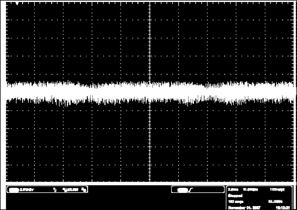
139 Figure 4-29 Measured output voltage (AC coupled) at rated power, 110Vrms Figure 4-30 Measured output voltage (AC coupled) at rated power, 180Vrms 121

140 4.7 Summary In this chapter, the Bi-flyback topology was re-analyzed and all the design curves and the design procedures were presented. In the design process, it was demonstrated that the peak direct power delivered to the output should be controlled by design not to exceed the output power. If this should occur, the output voltage will be contaminated with voltage ripple at double line frequency. The design curves have quantified the trade-offs between bus voltage, the percentage of direct energy transferred to the output, semiconductor voltage / current stress, overall size of the magnetic components, power factor, and total harmonic distortion. This provides the designer a complete set of tools to develop optimal design points for any application. On the other hand, the analysis revealed some limitations due to the dependency between input voltage and various design parameters. For the example, in the universal input application, the power factor and THD will be at their worst at low line. The maximum bus voltage will occur at the highest input voltage and critical load. The most important limitation is related to the peak direct energy that supplied to the output. The design has to accommodate worst case scenarios in both at the lowest line voltage and highest line voltage. The peak power directly delivered to the output through the flyback Mode will occur at the highest line voltage, while the peak direct power in the boost Mode will occur at the lowest line voltage. Limiting the peak power at both of these extremes will lead to lower direct power transfer. 122

141 While this limitation will not eliminate the suitability of the converter for universal line application, it will only make it more attractive for applications with narrower voltage range. The experimental efficiency measures near 84%, while keeping tight output voltage regulation, limited bus voltage, and complying with PF and THD regulation limits. As a future research topic, the converter should be analyzed when the output stage is operating in DCM. An optimal design point might be when the output stage is operating in CCM during a portion of the line cycle and in DCM during the other portion. This operation mechanism might also alleviate the issue of direct energy transfer variation with the input voltage. Another interesting topic could be analyzing the converter operation while considering the leakage inductor s effect on the flyboost operation. The presence of the leakage inductor will alter the operation of the input stage and might affect the design of the converter. 123

142 CHAPTER 5 AVERAGE MODELING AND AC ANALYSIS OF PFC CONVERTERS 5.1 Introduction Modeling and simulation play an important role in the design of power electronic systems. The classic design approach begins with an overall performance investigation of the system, under various conditions through mathematical modeling. This step is usually followed by computer simulation to verify the desired performance. Finally, prototyping should be carried out with several iterations of fine-tuning the system parameters. Unlike traditional DC-DC converters, variations in the line current, voltage, and duty cycle cannot be ignored in the AC-DC PFC converters [43-45]. The steady state operating point fluctuates significantly at double the line frequency. In single-stage converters, the controller aims to keep a good power factor while regulating the output voltage at the same time. The choice of average modeling to study both the large and small signal characteristics of the PFC converters should be considered, especially with its adaptability to computer simulation. In PFC converters, simulation for multiple line cycles is required to reach steady state. Average model simulation reduces the simulation time considerably, eliminates convergence difficulties, all while maintaining the ability to study the dynamics of the system. The modeling of PFC converters has not been studied thoroughly. In fact, many engineers and researchers adapted the popular averaging 124

143 technique for the analysis of DC-DC converters to the modeling of AC-DC systems. One of the most well known approaches is the state-space averaging method. This method that can be applied to any PWM converter [46, 47]. While state-space averaging is a good systematic approach, it depends on a long mathematical calculation and matrix manipulation. Recent contributions were also reported to enhance the model characteristics in Discontinuous Conduction Mode (DCM), and to extend the model to include components parasitics [48, 49] Since the development of the state-space averaging approach, the concept of averaging has been explored extensively, and among the important contributions was the three-terminal PWM switch, shown in Figure 5-1(a) [50, 51]. Unlike state-space averaging, the PWM switch model solely follows a circuit oriented approach. In this approach, only the non-linear components are encapsulated by the three-terminal model and all other components are left untouched. This sharp contrast with the state-space averaging method made this topology independent model very popular. In addition, the PWM switch approach improves the accuracy of the DCM dynamics in the high frequency range. And finally, the model comes directly with a convenient circuit form which makes it particularly suitable for use in circuit simulation tools. Another important contribution in the average modeling arena was the Generic Switched Inductor model (GSIM) [52-54]. The GSIM, Figure 5-1(b), 125

144 used well-defined mathematical equations to control Behavioral dependent sources. The unified model was efficient in modeling all the basic converters on the simulation platform, including the non-ideal parasitic resistance of the source, MOSFET, and the output capacitance ESR. What makes the GSIM stand out are its simple concept and the ability to switch between Continuous Conduction Mode (CCM) and Discontinuous Conduction Mode (DCM) in a seamless fashion, unlike the PWM switch model where the model is defined for CCM or DCM operation separately. This advantage overcomes the severe limitation other models experience during time domain simulation at wide load changes or during the simulation startup transient. (a) (b) Figure 5-1 Switch Models (a) PWM Switch, (b) GSIM 126

145 The three-terminal networks mentioned encapsulate the switching elements and help in the investigation and rapid prototyping of the DC-DC converters. Other methods have also been reported in literature to aid in the simulation process [55, 56]. However, these models, while extremely useful, have a prerequisite for their use - the three-terminal network must be identified in the circuit. In the example of the single-stage PFC converters, such as the bi-flyback converter in Figure 5-2 [29, 57], there is usually more than one passive switch and it is usually separated from the active switch by the High Frequency (HF) transformer. As a result, in this example, the threeterminal cell is hard to conceptualize, especially if the leakage inductance is considered. As such, various assumptions and approximations are generally used to get past this difficulty, often sacrificing accuracy in the process. In this situation, the conventional approach of finding such a switch or equivalent switch needs to be modified and a more generalized PWM switch should be investigated. Previous attempts to model single-stage PFC converters was limited to topology specific models [58-63]. This is due to the limitation of the existing general average models and their ability to accommodate a complex structure. 127

146 T 1 n 1 :1 D 2 V in T 2 n 2 :1 D 1 C 0 V O S V DS C S V CS Figure 5-2 The Bi-flyback PFC Converter This chapter presents a more generalized five-terminal switching network model that is capable of modeling DC-DC, AC-DC, and the more complex single-stage PFC converters. Since the flyback structure can be often found in PFC converters either as the front-end PFC or the output stage, the proposed model shown in Figure 5-3 encapsulates the flyback transformer, taking in account the leakage inductance, an intermediate bus input, and can address both CCM and DCM operation. It will be shown that the derived model can be easily implemented in a PSPICE subcircuit to facilitate steadystate and transient analysis and yield fast simulation with high accuracy. In addition, the model will help investigate the dynamic response of the system. The introduced model is general and can be easily used to model many converters. Further, this model is the first model that takes the leakage inductance effects in consideration, which is particularly important when the leakage inductance plays a role in the topology operation. Previous results 128

147 have highlighted the significant impact of the leakage inductance on the basic flyback converter operation in both the time and frequency domains [64]. in i in out bus i bus E lm L m L k E lk i o im i k GNDpri GNDsec i in n :1 L k D 1 L m i m C o R o D 2 i bus Figure 5-3 The Proposed Five-terminal Switched Transformer Model 129

148 5.2 The Switched Transformer Model (STM) Principle of Operation The basic principle in developing all average models is that the average inductor current can be generated from the average voltage across the inductor during a switching period, or simply the differential equation for the inductor current and voltage relation can be rewritten in terms of average values as in eq. (1). di() t L v () L t dt = (5.1) Assuming the average voltage across the inductor will not change significantly during the switching cycle and the switching period is much smaller than the basic time constant of the converter system. To derive the average voltage for the inductor we should consider the various possibilities of the inductor current waveforms. For the basic nonisolated topologies operating in CCM, the average voltage can be described as a function of the voltage across the terminals and the time the switch stays ON or OFF. For the boost converter, as an example, the average voltage can be expressed by, E = V D + ( V V ) (5.2) L in on in out D off 130

149 In the proposed model, the voltage equation is more elaborate due to presence of two inductors, Lm and Lk. These inductors describe the magnetizing and leakage inductances respectively. In addition, it has more than the simple CCM or DCM operation, where ideally there are four combinations when each inductor operates in either CCM or DCM. For generality, the model will also consider the case when the magnetizing inductor does not discharge to the output, but will instead act as a boost inductor in series with the leakage inductance and discharge to the bus. This case can happen often during start up, heavy bus load, or due to a special PFC operation mechanism we will see in the following sections. The development will refer to the case where the magnetizing inductance discharges to the output as the Flyback Mode, and the Boost Mode when it discharges to the bus as shown in Figure

150 Vin n 1 :1 i o + Vo Vin n 1 :1 + Vo i o i o Vbus Vbus Vin n 1 :1 + Vo Vbus Figure 5-4 Flyback versus Boost Operation After deriving the inductors voltage equations the model will generate the average inductor current using basic circuit operators as shown in Figure 5-3. Then, the average terminal currents will be derived from mathematical relations between the average inductor current, the transformer turns ratio, and the duty cycle. The last step in developing the average model is modeling the duty cycle using algebraic behavioral equations. As mentioned in the introduction, the model should automatically switch between various CCM and DCM operational combinations depending on the converter parameters and 132

151 terminal voltages. In order to address these complex Modes of operation, the proposed model will define several time periods as depicted in Figure 5-5. DonTs: Time duration where the main switch is conducting DoffTs: Magnetizing inductor discharge time. DlkTs: Leakage inductor discharge time. DoutTs: Time duration between the turn on of the main switch and the moment the leakage and magnetizing inductor currents are equal. i m t i k DonT DT s lk s D T out s D T off s T s t Figure 5-5 Time Duration Definition of the Proposed Model 5.3 The Switched Transformer Model (STM) Operation Modes In this section, the operating Modes of the proposed model are discussed in detail. The main objective when creating a good average model is to 133

152 accurately identify all the possible combination of Modes with their associated charging and discharging voltages for the leakage and magnetizing inductors. This is done in order to derive the generalized equations. For simplification, the operating Mode is defined by the current conduction Mode of the magnetizing inductor followed by the leakage inductor of the switched transformer model. For example, flyback CCM+DCM means that the transformer operates like a flyback transformer, with magnetizing inductor operating under CCM and leakage inductor operating under DCM, while boost DCM+DCM means that the transformer s leakage and magnetizing inductors operate as a simple boost inductor and both are in DCM. All the waveforms associated with the Modes of operation are shown in Figure ) Flyback DCM-DCM: At light load, the flyback transformer magnetizing and leakage inductors currents are discontinuous. For this case, we can identify four operational intervals as follows: Interval 1 (t o ~ t 1 ): S is turned on at to. The input voltage, Vin, is applied to primary winding of the flyback transformer, which includes the magnetizing inductor Lm and the leakage inductor Lk. The input voltage across each inductor is voltage divided according to the inductance value. The current in both inductors is identical since both inductors operate in DCM with the same charging slope. 134

153 Interval 2 (t 1 ~ t 2 ): S is turned off at t1. The magnetizing inductor discharges to output through the transformer secondary winding, while the leakage inductor discharges through the Vbus terminal. At t2 the leakage inductor current reaches zero and D2 disconnects. Interval 3 (t 2 ~ t 3 ): The magnetizing inductor continues to discharge to the output until its current reaches zero at t3. Interval 4 (t 3 ~T S ): During this interval, there is no current following in the model. The main switch S is turned on again at TS, and a new switching cycle begins. 2) Flyback CCM+DCM: When the load increases, the current through the magnetizing inductor becomes continuous, while the current through the leakage inductance, Lk, is still discontinuous because of the difference in inductance value. As shown in Figure 5-6(b), the leakage inductor will cause some delay for the current transition between transformer primary and secondary windings. Interval 1 (to ~ t1): S is turned on at to. The input voltage Vin is applied across the magnetizing and leakage inductors, Lm and Lk. The current im continues to discharge with initial current, Im2, while ik will start charging from zero. The difference between the magnetizing and leakage currents reflects to the secondary of the flyback transformer. At t1, the leakage and magnetizing currents become equal. 135

154 Interval 2 (t1 ~ t2): At t1, Vin will charge Lm and Lk according to their inductance values. The charging will end when the S is turned off at t2. Interval 3 (t2 ~ t3): im and ik will discharge to the output and bus terminals respectively. At t3, ik will reach zero and D2 will disconnect. Interval 4 (t3 ~TS): As in flyback DCM+DCM. 3) Flyback CCM-CCM: During start-up or at high load on the bus terminal, the non-ideal flyback converter may enter a condition at which both the leakage and the magnetizing inductors operate in CCM. As shown in Figure 5-6(c), there are three operation intervals in this Mode, Interval 1 (t o ~ t 1 ): S is turned on at to. The input voltage Vin is applied across Lm and Lk. while im and ik will start with initial currents Im2 and Ik3 respectively, the current in magnetizing inductor is higher and until t1, a current-transition interval exists until both currents are equal. Interval 2 (t1 ~ t2): As in flyback CCM+DCM Interval 3 (t2 ~ TS): At t2, the main switch is turned off. The magnetizing inductor is discharged to the output through the transformer secondary winding, while the leakage inductor is discharging through Vbus. At Ts another switching cycle starts. 4) Boost DCM-DCM: During start-up, heavy load on the bus terminal, or for PFC application, the non-ideal flyback converter may operate like a boost 136

155 converter without any current transferred to secondary output. This Mode is self explanatory from its waveforms in Figure 5-6(d). 5) Boost CCM-CCM: Under this Mode, the transformer primary winding operates like a typical CCM boost inductor. This Mode is also self explanatory from the waveforms in Figure 5-6(e). i m I m1 Vin L + L m k nv L m o t i k I m1 Vin L + L m k ( Vbus Vin nvo ) L k t i o t i bus D T on s D T DT t0 t 1 t2 3 off lk s s t Ts t (a) Flyback DCM+DCM 137

156 i I m 1 m Vin L + L m k nv o L m I m2 t i k I m1 Vin L + L m k ( Vbus Vin nvo ) L k I m2 t i o V in + nv L k o DT lk s t i bus D T D T on out s s t0 t 1 t2 3 t Ts t (b) Flyback CCM+DCM 138

157 i I m 1 m Vin L + L m k nv L m o I m2 t i k I m1 Vin L + L m k ( Vbus Vin nvo ) L k I k3 I m2 t i o V in + nv L k o t i bus D T out s D T on s t t t0 t 1 2 Ts (c) Flyback CCM+CCM 139

158 I m1 i m Vin L + L m k V L bus m V + L in k t i k I m1 Vin L + L m k V L bus m V + L in k t i o t i bus DonTs Doff Ts t0 t 1 2 t Ts t (d) Boost DCM+DCM 140

159 I m1 i m Vin L + L m k V L bus m V + L I m2 in k t i k I m1 Vin L + L m k V L bus m V + L in k t i o t i bus D T on s t t0 t 1 Ts (e) Boost CCM+CCM Figure 5-6 Primary and Secondary Current Waveforms in the Flyback and Boost Modes 5.4 Unified Model Equations By careful inspection of the waveforms discussed in the previous section, it was determined that it was possible to merge all the operational Modes together under a unified model. The basic method for constructing this average model is to find the average voltage applied to each inductor, and the 141

160 average current through each terminal. The known parameters in the model include the inductors values, the terminal voltages, the duty cycle Don, and the switching frequency. Based on these parameters, all the variables for the model will be derived in a general form in this section. The unified model equations in this section represent a set of equations that can be solved numerically inside a simulator that provides this capability, such as PSPICE, or even general mathematical software like MathCAD. A. The Average Inductors Voltage Equations Based on the waveforms in Figure 5-6, the charging voltage for both the magnetizing and leakage inductances is simply a voltage division of the input voltage across Lm and Lk. However, unlike the charging voltage, the discharging voltage is different between the flyback and boost Modes. In order to identify the general relationship, we have to consider the voltage across D1 in Figure 5-3. D1 will stay on if: nv o L ( V V ) < m bus Lm + L k in (5.3) If this inequality is true then the model operates in the flyback Mode and hence Lm will discharge by nvo, otherwise the model is operating in the boost Mode. Based on this observation, the following equations represent the unified discharge voltages for the inductors: 142

161 V = Lm min ( V ), Lm + L V nv o k lm bus in Lk V = max ( V V ), V Lm + Lk lk bus in bus in V nv o (5.4) (5.5) Hence, the average voltage can be obtained by the following equations: E ( ) LV D D = + V ( D D out ) + m in on out Lm lm off Lm + Lk (5.6) ( ) LV D D E = + D ( V + nv ) + V D leak (5.7) k in on out Lk out in o lk Lm + Lk Eqs. (5.6) and (5.7) are valid representations of the average voltage across the Lm and Lk in all Modes. While Dout is not present in some Modes its value is equal to zero and the equations are still valid. B. Time Intervals and duty-ratios Calculation In the above voltage equations Doff, Dleak, and Dout need to be identified and modeled in general equations that are valid for all the waveforms in Figure 5-6 and a function of the control input, Don. If the magnetizing current operates in CCM, Doff will be 1-Don. In DCM, the discharge time can be derived using the peak and average inductor 143

162 current values. The generalized equation can be described by the following equation, D off ( + ) 2Im Lm L k = min 1 DON, D on VDT in on s (5.8) using the same methodology, the Dleak generalized equation is, D 2I I D k m2 on leak = min 1 DON, + Dout Im 1 D on (5.9) The current transition period occurs in the flyback CCM-DCM and CCM- CCM, can be calculated from as follows, D out = ( Im2 Ik3) ( V + nv ) in o L T k s (5.10) We can notice that Dout is equal to zero if Im2=Ik3, and hence Eq. (5.10) is valid for all Modes in Figure 5-6. C. Minimum and Maximum Currents values The duty ratio equations described above require some peak and minimum inductor currents equations. The following equations were derived in a general form, 144

163 I Lm = + m1 D on I + D off Vin ( ) on out 2( L + L ) D D T m k s (5.11) I m 2 = D on I Lm + D off Vin ( ) on out 2( L + L ) D D T m k s (5.12) I k 3 = 2 I I D I ( D D ) Lk m2 on m1 on out +D leak D leak + D out (5.13) D. Average Current Equations To finalize the generalized model equations, the average input and output current quantities can be derived from the inductors average currents as follows, I in = I (5.14) Lk I o = n( I I ) (5.15) Lm Lk Finally, the average bus current can be derived from the leakage inductor current waveform as: I = bus + I D m1 k3 leak ( I ) 2 (5.16) E. Average Model Implementation 145

164 The derived equations (5.4) to (5.16) can be directly implemented using the ABM function blocks in PSPICE, as shown in Figure 5-7(a). This circuit can be masked under a simple subcircuit block as shown in Figure 5-7(b) that can be used to model many topologies as will be demonstrated in the upcoming sections. (a) Average Model Equations 146

165 Flyboost IN OUT BUS GND D LM = {L1} FS = {Fs} LK = 10u N = {n1} (b) Sub-circuit Block Model Figure 5-7 Average Model implementation in Pspice 5.5 Average Modeling Applied to the Bi-Flyback Converter The Bi-flyback single-stage PFC converter consists of two flyback transformers, as shown in Figure 5-2. In this topology, the input flyback transformer, T1, has a special boost operation period depending on the instantaneous value of the input line voltage as shown in Figure 5-8. In the flyback Mode, the two circuits operate independently while in the boost Mode all the current from the PFC cell flows through the primary winding of the DC-DC cell transformer and then to the output. 147

166 T tx 2 t T T x 2 2 +t x T t x T Figure 5-8 Operational Modes of the Bi-flyback Converter during One Line Period After a careful study of the Bi-flyback converter operation, the STM was used to model the PFC cell because of the important role of the leakage inductance during the transition between the flyback and the boost Modes. The DC-DC cell was modeled using a DC-transformer model. This way, the operation of the two flyback circuits is separated, and the average model of the Bi-flyback converter can be developed easily from the basic models. The final average model is shown in Figure 5-9(b), where an ideal transformer, T1, is used to connect the two cells in a manner that mimics the actual circuit operation. 148

167 in Lk 10u LCHOKE1 {L1} Din Vds Vout ABS V1 S3 Vsw Sbreak LMAIN1 {L2} Cs 470u IC = {Vcs_IC} Vcs D1 LMAIN2 {L2/n2/n2} D2 LCHOKE2 {L1/n1/n1} RCo 7m Co 1000u IC = 20 RLoad 5 K K2 K K1 K_Linear COUPLING = 1 K_Linear COUPLING = 1 L1 = Lchoke1 L1 = LMAIN1 L2 = Lchoke2 L2 = LMAIN2 PARAMETERS: L1 = 50uH n1 = 5.5 L2 = 200uH n2 = 5 Vcs_IC = 155 Vp = 110 f s = 100k Verr =.5 V2 PER = {1/f s} TR = {1/fs-15ns} V2 = RC 1Meg Verror 0 CC1 10n RC2 20k CC2 170p F1 Vref V3 20 CC3 4.7n RC1 10k RC3 1.8k 0 (a) Switching Model Vin ABS in Flyboost IN T1 BUS GND OUT D LM = {L1} FS = {Fs} LK = 10u N = {n1} 0 D Ratio = {n2} RCo 7m Co 1000u IC = out RLoad 5 PARAMETERS: L1 = 50uH n1 = 5.5 L2 = 200uH n2 = 5 Vcs_IC = 168 Vp = 110 f s = 100k Verr =.5 Cc2 170p IC = -20 out Cs 470u 0 0 bus D FLYBACK IN OUT D GND LM = {L2} N = {n2} FS = {Fs} 0 0 D 1 V1 EA U5 Cc1 10nF IC = -20 V 0 Rc2 20k Vref 20 0 RC3 1.8k CC3 4.7n RC1 10k (b) Average Model Figure 5-9 The Bi-flyback PFC Converter Switching and Average Simulation Models 149

168 A. Time-Domain Operation Both the switching and average models of Bi-flyback PFC converter were used to perform a time domain analysis and the simulation results were compared. The average model simulation discards the high frequency effects during the individual switching cycles, allowing fast simulation for the model. As a result, the simulation for several line cycles is possible within a short amount of time. For comparison purposes, the Avgx function was used to obtain the average waveforms from switching model. From the simulation results in Figure 5-10, it is clear that the switching and the average models correspond very well to each other. In addition, the switching simulation took additional simulation time and many convergence problems in PSPICE needed to be addressed due to switching nature. This can highlight the benefits of the proposed average model as a viable simulation tool. (a)switching Model Simulation Results 150

169 (b) Switching Model Simulation Results (Averaged) (c) Average Model Simulation Results Figure 5-10 The Bi-flyback PFC Converter Simulation Results 151

170 B. AC operation The model of Figure 5-9(b) was used in the AC analysis except the sinusoidal input voltage source was replaced by a DC voltage source to represent the instantaneous input voltage at a specified simulation time. The simulation model was also adjusted to match the experimental circuit in the following section (output capacitor value, leakage and magnetizing inductance, and output load). The frequency response was simulated at different input voltages (90V to 170V with 10V increments). The control to output transfer function is shown in Figure As shown in the results, the gain of the transfer function was changed at different intervals during one line cycle. The maximum gain happens when the input voltage reaches its peak value. The variation as a function of input will be considered during compensator design. 152

171 Figure 5-11 Control to Output (V o /d) Frequency Response Simulation Results Bi-Flyback by Average Model 5.6 Experimental Results To verify the modeling results, a prototype of the biflyback converter in Figure 5-10 was tested and its frequency response was measured using Venable frequency analyzer. For completeness, Table 5-1 outlines the converter specifications, efficiency, and the PF. The experimental results in Figure 5-12 represent the control to output voltage transfer function (V o /d). There is great agreement in the shape between the experimental and simulation results in Figure

172 Table 5-1 Converter Specification and Performance Input Voltage Output voltage Output Power Switching Frequency Measured Efficiency Measured PF Universal (85-265Vac,rms) 20V 90 W 100kHz 90W and 110Vac,rms input 90W and 110Vac,rms input To illustrate the measurement procedure, Figure 5-13 outlines the measurement setup. The frequency analyzer oscillator (OSC) was connected directly to the DSP Analog to Digital Converter (ADC), and an appropriate DC level from the OSC output was used to setup the needed DC operating point. The DSP was configured to convert the ADC reading linearly to a corresponding duty cycle on the DSP PWM output that was connected to driver and then directly to the main switch. The converter DC operating point was perturbed by the analyzer OSC and the output voltage was modulated accordingly. Before the final measurements were done, the DSP frequency response was measured and the final measurements were adjusted to compensate for the DSP gain. It is to be noted that the results in Figure 5-12 are obtained using an open loop frequency measurement to eliminate any potential mismatch in the compensation network that might result from using the DSP. During the experiment, parasitic elements and noise in the 154

173 developed prototype caused many difficulties in measuring the response at rated power. Hence, the load was changed from 5 to 10 ohms in order to attain presentable results. The graph in Figure 5-12 consists mainly of a first order pole and a left half-plane zero. In addition, a high frequency delay is present, due to unknown parasitics and sampling effects. It was also noticed that the pole position depends on the load and the output capacitance, while the zero depends on the output capacitance and ESR value. Figure 5-12 Experimental Control to Output Voltage (V o /d) Frequency Response measured for the Bi-flyback PFC converter 155

174 Figure 5-13 Frequency Response Measurement Setup 5.7 Summary In this chapter, a five-terminal switched inductor model was proposed and its generalized equations were derived. The proposed model is capable of modeling the single-stage PFC converters with more accuracy since it includes more terminals to accommodate its complex structure. In addition, the model also takes in consideration the leakage inductance of the transformer for more accurate time and frequency domain analysis. The proposed model was applied to the Bi-flyback converter and its time domain waveforms match the switched simulation results with great accuracy and were more than fifty times faster to create. Small-signal analysis forms the basis for effective control loop design; the proposed model enables easy frequency response analysis for the single-stage PFC converters, an area that has been overlooked in the past. The developed frequency response analyses show good agreement with the experimental results. The mechanism 156

175 presented in this chapter enables rapid simulation, supports AC small signal analysis directly, and most importantly, produces a comprehensive investigation of a converter topology that cannot be modeled by existing approaches. 157

176 CHAPTER 6 ANALYSIS, DESIGN, AND OPTIMIZATION OF THE CENTER-TAPPED FLYBACK CONVERTER 6.1 Introduction This chapter presents a new topology to be analyzed based on direct energy transfer concept. The bi-flyback converter was able to deliver energy directly to the output during the flyback Mode and the boost Mode, but at the same time input power factor will degrade when more energy is delivered to the output directly. Also the converter was not able to deliver maximum power evenly during universal line input voltage, which will result in less than optimal efficiency results. This chapter focuses on another topology that can alleviate these issue and promises good results for universal line input voltage applications. 6.2 Principle of Operation In this section, the principle of operation of the center-tapped flyback converter will be examined. As shown in Figure 6-1, the converter consists of a BIFRED flyback converter that was modified by adding an additional winding to the main transformer in series with the main switch. This modification will serve many purposes. First, it will allow the input inductor changing current to be stored in the additional winding and then to be transferred directly to the output. Second, by changing the turns ratio, n 1 :n 2, 158

177 the current can be steered away from the main switching to the other branch of the flyback inductor, this will reduce the current stress and improve the converter efficiency. In addition, the added winding will introduce a bus voltage feedback mechanism that will automatically limit the voltage on the bus capacitor, Cs. On the other hand, the new circuit has added complexity due the introduced winding. This new design dimension has to be analyzed and a proper design procedure has to be developed to maximize the utilization of the new topology. V in D in L in n 1 :1 n 2 :1 D + C V O S C S + V CS i s (a) Derivation and Concept Illustration 159

178 V Cs + C s i Lm N p :1 D n 2 V in D in i Lin L in L m i p2 i p1 C V O n 1 S i s (b) Rearranged for Clarity Figure 6-1 The Center-Tapped Flyback Topology The input line voltage dictates the operation of the topology and whether the input inductor will be engaged in the operation or not. This mechanism can be understood by considering the voltage across the input diode Din when the main switch S turns on. If the voltage across the diode is greater than zero, the diode will conduct and the boost inductor will charge through the tapped flyback transformer to the magnetizing inductor, and then discharges to the output directly. Otherwise, the diode will block the current flow and the converter will simply operate like a typical flyback converter supplying all the output power from the stored energy in the bus capacitor. The Mode the input inductor is not engaged will be called Mode 1, because it happens first during the line cycle. Later on the input inductor will be utilized during Mode 2. The conditions that govern this operation are given as, 160

179 vin(t) < (n1/np)vcs (Mode 1) (6.1) vin(t) > (n1/np)vcs (Mode 2) (6.2) Considering the converter operation during a line cycle, the converter will change the Mode of operation according to equations (6.1) and (6.2), this is further illustrated in Figure 6-2. Due to the nature of the operation, the conduction angle of the converter is limited unlike the bi-flyback converter described in previous chapters. This can impact the power factor of the converter if not properly designed. The boundary Mode condition happens at tx, which can is given by, 1 n 1 V Cs t x w asin N p V p (6.3) Figure 6-2 Modes of Operation during a Line Cycle 161

180 In the following subsections the converter operation will be analyzed based on its Modes of operation. The following assumptions will be considered during the analysis, Lin is assumed to be operating in DCM to achieve automatic PFC Lm is assumed to be operating in CCM to reduce the peak current in the DC-DC converter Ideal components without parasitic parameters such as leakage inductance of the transformer, on resistance of the switching devices, etc. The input voltage will be considered constant during a switching cycle Constant output voltage through tight regulation Mode 1 Operation During Mode 1, the input diode, Din, will be off and the converter will operate like a typical flyback converter charging the magnetizing inductance of the transformer, Lm, from the bus capacitor and then discharging its energy to the output. The DC-DC converter will deliver the needed power from the storage capacitor to the output to keep tight output regulation. During this Mode, there are two time intervals that characterize the converter operation, as shown in Figure 6-3. The associated waveforms for these intervals are shown in Figure

181 V Cs + C s i Lm N p :1 D n 2 V in D in i Lin L in L m i p2 i p1 C V O n 1 S i s (a) Interval 1 (t o -t 1 ) V Cs + C s i Lm N p :1 D n 2 V in D in i Lin L in L m i p2 i p1 C V O n 1 S i s (b) Interval 2 (t 1 -T s ) Figure 6-3 Equivalent Circuits for the Three Intervals during Mode 1 163

182 Figure 6-4 Key Waveforms during Mode 1 Operation Interval 1 (t0-t1): The switch is turned on at t0. The magnetizing inductor current, ilm, is charging linearly from the bus voltage, while the same current flows through primary windings. The following expressions are obtained for the main waveforms, 164

183 i Lm () t V CS t t L o m ( ) i + Lm T s ( ) (6.4) i p1 i Lin i p2 i D 0 (6.5) Interval 2 (t1-ts): The switch turns off at t1 causing the magnetizing inductor current, ilm, to discharge though the primary winding to the output through D. The following expressions are obtained for the main waveforms during this interval, i Lm () t N p V o t t L 1 m ( ) i + Lm t 1 ( ) (6.6) i p2 () t i Lm () t i p1 () t (6.7) n 2 V o i Lm2 () t i p2 t t 1 L m2 ( ) i Lm2 ( t 1. ) + (6.8) i D () t N p i Lm () t (6.9) where Np=n1+n Mode 2 Operation When t>tx, Din starts to conduct when the switch turns on and the converter enters operation Mode 2. The main difference between the two Modes is the engagement of the input boost inductor in the operation. During 165

184 this Mode, the bus capacitor energy should be recovered to maintain steady state operation. In addition, the input power will be directly transferred to the output in this Mode. The amount of the direct energy transferred to the output will ramp up with the input voltage and then be capped at the output power level. V Cs + C s i Lm N p :1 D n 2 V in D in i Lin L in L m i p2 i p1 C V O n 1 S i s (a) Interval 1 (t o -t 1 ) 166

185 V Cs + C s i Lm N p :1 D n 2 V in D in i Lin L in L m i p2 i p1 C V O n 1 S i s (b) Interval 2 (t 1 -t 2 ) V Cs + C s i Lm N p :1 D n 2 V in D in i Lin L in L m i p2 i p1 C V O n 1 S i s (a) Interval 3 (t 2 -T s ) Figure 6-5 Equivalent Circuits for the Three Intervals during Mode 2 167

186 Figure 6-6 Key Waveforms during Mode 2 Operation Interval 1 (t0-t1): The switch is turned on at t0. The magnetizing inductor current, ilm, is charging linearly from the bus capacitor voltage as in interval 1 in Mode 1. However, ilin is also charging from the input rectified voltage in Mode 2. The input current will be divided between the primary windings according to their turns-ratio. The input current will offset the charging current from the bus capacitor. Further, at higher input voltages the input current will also charge the bus capacitor. The equations that describe the main current waveforms are similar to the interval 1 equations in Mode

187 i Lm () t V CS t t L o m ( ) i + Lm T s ( ) (6.10) i Lin () t n 1 V g V N Cs p t t L o in ( ) (6.11) i p1 () t i Lin ()n t 1 N p (6.12) i p2 () t i Lin ()n t 2 N p (6.13) i Cs () t i Lm () t i p2 () t (6.14) where Vg is the instantaneous input voltage, which is assumed to be constant during the switching interval. Interval 2 (t1-t2): The switch turns off at t1. Unlike in Mode 1, the input current is already charged through the input diode, Din. This will force the boost inductor current, ilin, to discharge through the second primary winding, n2. At the same time, this current will be reflected directly to the output without having to be processed through the main switch. The input inductor discharging current will also flow to charge the bus capacitor. The magnetizing inductor current will discharge from the reflected output voltage. This interval ends when the input inductor current discharges to zero. The following expressions are obtained for the main waveforms during this interval, 169

188 i Lm () t i Lin () t V o N p t t L 1 m ( ) + i Lm ( DT s ) (6.15) V g V Cs n 2 V o t t L 1 in ( ) + i Lin ( DT s ) (6.16) i p1 () t i Lm () t (6.17) i p2 () t i Lm () t + i Lin () t (6.18) i D2 () t i o () t n 2 i p2 () t (6.19) i Cs () t i Lin () t (6.20) Interval 3 (t2-ts): The operation of the converter in interval 3 is similar to interval 2 of the Mode 1 operation. 6.3 Steady State Analysis This section will address the steady state operation of the center-tapped flyback converter over the input line cycle. While the analysis in the previous section shed some light on the converter operation in steady state, this analysis was based on the switching interval. Since the converter will be operating from a varying input voltage, the analysis will be expanded here to uncover the important relations and equations that govern the converter operation during the line cycle. For example, one of the most important parameters for the circuit design is the bus voltage across the storage 170

189 capacitor, Cs. In order to derive the VCs equation, the energy balance equation should be derived across the line cycle. During the following analysis, the following assumptions will be made: Ideal components, without parasitic parameters such as leakage inductance of the transformer, on resistance of the switching devices, etc. The input voltage will be considered constant during a switching cycle The switching frequency in much higher than the line frequency The DC bus voltage is constant during the entire line cycle. Constant output voltage through tight regulation Due to the symmetry of the power waveforms, the energy calculations will be performed on quarter line cycle for simplification Duty Cycle When operating in CCM, the duty cycle of the switch will remain constant during a line cycle, when tight output regulation and constant bus voltage is assumed. The duty cycle equation is given by, NV D P o = V N Cs + P V o (6.21) 171

190 6.3.2 Intermediate Bus Voltage In steady state, the energy discharged from the capacitor during a line cycle in Mode 1 should equal the energy that was used to charge the capacitor in the Mode 2, the expression for capacitor charge balance is, W W = (6.22) M1 M2 Cs_discharge Cs_charge During Mode 1, it is easy to calculate the energy supplied by the storage capacitor by considering the average charging current in the magnetizing inductor. The energy discharged from the bus capacitor can be calculated by integrating the average power during a switching cycle over the time of Mode 1. V I D W = N (1 D ) M 1 Cs o Cs_discharge p t x dt (6.23) 0 In Mode 2, the charging energy to the storage capacitor can be calculated based on the average capacitor current according to the Mode 2 analysis as follows, T/4 M2 n1 W Cs_charge =V Cs i t Lin_avg_charge + ilin_avg_discharge ilm_avg_charge x N dt (6.24) p 172

191 based on Eqs. (6.23) and (6.24), Eq. (6.22) can be rewritten as, t x I o D V Cs dt N p ( 1 D) 0 T 4 V Cs t x D 2 T s n 1 n 1 V 2 L p sin( w t) V in N Cs... p N p 2 n 1 D 2 V T p sin( w t) V s N Cs p L in V Cs + n 2 V o V p sin( w t) I o D + N p ( 1 D) n 2 D N p ( 1 D) d t... (6.25) DCM Condition for the Input boost inductor In order to achieve high power factor, the PFC inductor, Lin, should operate in DCM during the entire line cycle. The worst case scenario happens when the input voltage is at its peak value, or at t=t/4 as shown in Figure 6-7. At the time the current in the boost inductor is the highest, the inductor is guaranteed to stay in DCM if the DCM condition was satisfied at that time. The main condition for DCM operation during that switching cycle is, t2 t1 (1 D) T s (6.26) 173

192 I.Lin_ave_M2 () t t T 2 Figure 6-7 Average Input Current during Line Cycle At t=t/4, the converter will be operating in the Mode 2. By applying the equations for that interval, Figure 6-6, and substituting vin=vp, Eq. (6.26) can be rewritten as, V Cs n 1 V p V N Cs p + n 2 V o V p 1 D D (6.27) CCM Condition for the DC-DC Cell According to Mode 2 operation, the minimum load on the DC-DC converter will happen at t=t/4, when the input inductor providing the maximum direct output current as shown in Figure 6-8. In order to guarantee CCM for the DC-DC cell, it should be operating in CCM at that time instant. The necessary CCM condition can be found from Figure 6-6 as, Lm_avg s DI Lm 2 I (T /4) (6.28) 174

193 I.Lm_ave_M2 () t t T 2 Figure 6-8 Average Flyback Magnetizing Current during Line Cycle Expanding Eq. (6.28) in terms of the circuit parameters will yield the following equation for the critical inductance, I o n 2 L m_crit D 2 T s 2 L in 2 n 1 V p V N Cs p V Cs + n 2 V o V p ( 1 D) N p (6.29) 6.4 Design Equations and Methodology The main design parameters for the single-stage, center-tapped flyback circuit are: n1, n2, Lin, and Lm. From the previous sections, the main equations that can be used in the design are Eqs. (6.3), (6.21), (6.25), (6.27), and (6.29), for the transition time, tx, duty ratio, D, bus voltage, VCs, and the critical inductance for Lin and Lm respectively. In order to properly design the converter, the interaction and dependency between these variables will lead to a multi-dimensional design process that needs further investigation to highlight the trade-offs. 175

194 6.4.1 Main Equations and Design Curves Unlike the bi-flyback topology in CHAPTER 4, the center-tapped flyback topology does not suffer from the potential problem of delivering high peak power to the output. In this topology, there is no separate direct energy transfer path from the input to the output, and all power has to be processed through the coupled flyback inductor. As such, there is direct feedback for any excess energy through the voltage of the bus capacitor. This will limit the direct energy transferred naturally, and there is no need for design mitigation. In order to understand the design trade-offs, the following analysis will be carried out to create a comprehensive set of design curves for the converter under different conditions. A numerical solve block will be created to solve for VCs, D, tx, and Lin for a given value of Np and N, where N is the ratio between n2 and n1, as shown in Figure

195 Given T 4 V Cs t x D 2 T s 2 L in n 1 n 1 V p sin ( w t) V Cs + N p N p D 2 T s 2 L in 2 n 1 V p sin ( w t) V Cs N p 1 + V Cs + n 2 V o V p sin ( w t) n 2 D N p ( 1 D) I o D N p ( 1 D) dt t x V Cs 0 I o D N p ( 1 D) dt M D V Cs N p V o 1 M t x w asin n 1 V Cs N p V p N n 2 n 1 N p n 1 + n 2 n 1 V p V Cs N p 1 V Cs + n 2 V o V p 1 D D ( ) Find( V Cs, M D, ) SB N p, N :=,, t x, n 1, n 2 L in Figure 6-9 MathCAD Solve Block The solve block was used to generalize a set of design curves for the following circuit parameters: Vin,rms=110V, F=60Hz, Vo=20V, Po=70W, Fs=100kHz. The variations include different primary to secondary turns ratio, Np, and different primary winding turns ratio, N. Increasing N will result in more current redirected to the second primary winding, which will result in less current passing through the switch and more direct energy to the output The solve block will select the critical inductance for Lin. This will be further developed later on in this section since it reflects a maximum value. According to the results, the storage capacitor voltage is always constant and equal to the peak input voltage, V in this case. The bus 177

196 voltage will start to slightly increase when the input inductance starts decreasing. In the following discussion, the various design curves and trade-offs will be discussed. Primarily related to THD, PFC, direct energy transfer, size, MOSFET losses, and devices stress. A. Total Harmonic distortion and Power Factor One of the most important design trade-offs is the THD and PF values. The input current equation can be found from the steady -state analysis, then the THD and PF values can be obtained using Fourier analysis as outlined in the following Eqs. (6.30) to (6.36), T 1 I rms i t T in () t 2 d (6.30) 0 T 2 a 1 i t T in ()cos t ( w t)d (6.31) 0 T 2 b 1 i t T in ()sin t ( w t)d (6.32) C 1 a 1 + b 1 (6.33) I rms1 C 1 2 (6.34) THD i I rms I rms1 2 1 (6.35) 178

197 PF I rms1 I rms (6.36) In order to meet the regulatory requirement, such as IEC Class D, 45% THD and 0.9 PF are usually required. For this purpose, the THD and the PF curves were plotted in Figure 6-10 and Figure 6-11 respectively. As expected, the input current distortion decreases when Np or n increases. This is due to the boundary mode condition in (6.1). As the threshold voltage gets lower, the conduction angle will increase, which will increase PFC and reduce THD. It can be concluded from the graphs that Np of 2 and n of 3 or higher will be needed to satisfy the THD and PFC conditions THD n=1 n=2 n=3 n= Np Figure 6-10 THD versus Np for Different N Values 179

198 PF n=1 n=2 n=3 n=4 Np Figure 6-11 PF versus Np for Different n Values B. Direct Energy Transfer The direct energy transfer from the input to the output is one of the primary features of this converter. To quantify the amount of direct energy or power transferred to the output, the power delivered by the bus capacitor can be calculated in both Modes 1 and 2. Then, the total direct power transferred to the output can be found by subtracting output power from the power delivered from the bus, Eq. (6.37), the results are shown in Figure P in_direct () t P o P Cs_Direct () t (6.37) 180

199 P in_direct () t 200 P Cs_Direct () t + P in_direct () t P in () t 2 P o sin( 120 π t) t Figure 6-12 Direct Energy Transferred to the Output over Half Line Cycle By integrating the direct input power transferred to the output over a half line cycle, the graph in Figure 6-13 shows how the direct power transferred varies with turn ratios. Unlike the bi-flyback topology, improving the PF and THD coincides with increasing the direct power. According to Figure 6-13, the direct power transfer can reach 60% compared to 50% in the bi-flyback topology. There are some practical limitations on this number as will be shown in the following sections. 181

200 Direct Energy n=2 n=1 n=3 n= Np Figure 6-13 Direct Energy Transferred to the Output versus Np for Different n Values C. Main Switch RMS Current While it is desirable maximize the average power transferred directly to the output, the main drive for this topology is to reduce the losses and current stress on the switch. For this reason, the average RMS switch current during a switching cycle was derived and averaged over a line cycle. From there the conduction power results are plotted in Figure By observation, it is desirable to increase turns ratios to reduce the switch conduction losses, but actually the relation is not linear. Increasing the primary turns ratio from 1 to 4 will have a significant impact, but any further increase will have the opposite effect. Increasing n beyond 2 to 3 will have almost no difference in switch conduction losses. 182

201 Figure 6-14 Main Switch Conduction Losses versus Np for Different n Values D. Magnetic Component Size An important part of the design is to study the trade-offs in component sizing. In order to understand how the transformers and the input inductor size will be affected by the selection of Np and n values, these relationships were plotted in Figure 6-15-Figure 6-17, for Lin, and Lm respectively. In the figures we can see that enhancing the THD, PF and improving direct power transfer and switch losses will come with the ultimate price of increasing the size of the magnetic components, especially Lm where size rises sharply after increasing the turns-ratio above a certain level. 183

202 Figure 6-15 Lin Energy versus Np for Different n Values Figure 6-16 Lm Energy versus Np for Different n Values 184

203 Figure 6-17 Zoomed-in from Figure Stress Equations Stress equations are important for the sizing of the semiconductor components. The peak vaules ILm_max and ILin_pk will be used for this pupose, I Lin_pk_M2 () t n 1 v in () t V N Cs p L in I Lm_max_M2 () t I Lm_ave_M2 () t DT s + V Cs DT s 2 L m (6.38) (6.39) The MOSFET has to handle the maximum current in both magnetizing inductors summed together in addition to maximum input current reflected to the first primary winding. 185

204 I SW_pk () t I Lm_max_M2 () t I Lin_pk_M2 ()n t 2 + if t N x < t < p T 2 t x (6.40) I Lm_max_M1 otherwise The equation for the peak switch current is time varing during the line cycle, and the absolute maximum occurs at a different time instance depending on the design values as illustrated in Figure I SW_pk () t t Figure 6-18 Maximum Switch Current during a Line Cycle The output diode has to withstand an even higher peak current because of its location (on the low voltage side of the circuit). ( ) n 2 I Lm_max_M2 t I D_pk () t I Lin_pk_M2 () t + I Lm_max_M2 () t I Lm_max_M1 N p otherwise + ()n 1 if t x < t < T 2 (6.41) The voltage stress on the diodes and the switch are given by the following equations, V S_Max N p V o + V Cs (6.42) 186

205 V Cs V D_Max V o + (6.43) N p The MOSFET and diode stress equations can highlight the trade-offs between different designs. For that purpose, Figure Figure 6-21 was plotted to quantify the differences. Figure 6-19 shows how the voltage stress on the MOSFET increases with the primary turns-ratio Np, while the diode voltage stress decreases. While this graph was generated for a 110Vrms input, it should be noted the maximum stress will happen at 220Vrms in universal line applications. Voltage stress can reflect on the semiconductor device selection. Lower voltage devices tend to have better efficiency. This is especially significant when a schottky diode can be used at the output side. Figure 6-19 MOSFET and Diode Voltage Stress versus Np 187

206 The peak current stress on the MOSFET is shown in Figure While the voltage on the MOSFET will increase with primary turns ratio, the peak current will decrease. This will raise the question about switching losses where both the peak current and voltage will play a significant role. For that purpose, Figure 6-21 was plotted to evaluate the switching losses. It is clear that despite the increasing voltage stress, the overall losses will decrease while the primary turns-ratio is increased. Figure 6-20 MOSFET Peak Current Stress versus Np for Different n Values 188

207 Figure 6-21 MOSFET Estimated Switching Losses versus Np for Different n Values Design Example Table 6-1 highlights the main specifications for the design example, which are typical for notebook power supply. Table 6-1: Center-tapped flyback Converter Design Specifications Input Voltage Universal (85-265V ac,rms ) Output voltage 20V Output Power 70 W Switching Frequency 100kHz Measured PF IEC Class D 189

208 The curves in Figure Figure 6-17, can be used as the first step in a tradeoff study for this design. Starting from Figure 6-10 and Figure 6-11, we can see that we need Np > 2 to meet PF>90% and THD<0.45. For the case of Np = 2, the converter should utilize n > 3, or n > 2 for any other higher Np value, to comply with PF and THD requirements. Proceeding to Figure 6-13, we can get an idea about how the direct power transfer varies with the selection. For the options mentioned above, the direct power transferred to the output can vary from 50% to 60%. Now, proceeding to Figure 6-14 we can see that the optimum point for conduction losses is at Np=4, but these results were further expanded in Figure 6-21 to include switching losses. These losses tend to be more dominant in low power high voltage applications. Thus far, all the curves indicate a performance enhancement with increasing turns ratio, however size reduction will dominate and limits how far the turns ratio can be increased. According to Figure 6-15 to Figure 6-17, the size of the magnetic components will increase significantly with increasing turns ratio. This will practically eliminate any design choice with Np above 4. As can be established from the curves, the improvement will start to be very limited above Np=4, while the size penalty is increasing significantly. Another observation is a limited increase in size at lower Np values when n is increased. As a result, the design will be recommended for Np=2 and n=4 or Np=3 and n=3. The results of the analysis for the two design choices are shown below. 190

209 Table 6-2: Summary of Design Results Design 1 (Np=2, n=4, Lin=75μH, Lm=150μH) Design 2 (Np=3, n=3, Lin=100μH, Lm=340μH) Vcs 346V 360V % P Direct 54.4% 55% THD, PF 40.3, 92.7% 38, 93.5% I SW_PK 5.5A 3.9A I D_PK 10.54A 11.8A V SW_Max 386V 419V V D_Max 193V 140V L in energy (μh.a 2 ) L m energy (μh.a 2 ) Simulation Results The closed-loop PSPICE simulation of the proposed converter, Figure 6-22, has been carried out over one line cycle and the simulation results are show in Figure 6-23 to Figure It is clear from simulation waveforms that the theoretical and simulation waveforms correspond to each other in both the Mode 1 and the Mode 2. The input current waveform in Figure 6-26 promises high power factor and match the predicted shape. 191

210 Cs 50u IC = {Vcs_IC} 0 Cs RATIO = XFMR1 0 U1 2 I D1 V+ Vout V- Vin Lin 75u Din Vb L1 I 150u 1 0 U2 3 2 I ABS V1 VAMPL = {Vp*1.414} Vsw + - S3 + - Sbreak 1 3 XFMR1 RATIO I = 2.5 RCo 7m Co 1000u IC = 20 RLoad V2 1 Verror F1 CC3 4.7n RC3 1.8k PER = {1/f s} TR = {1/f s-15ns} V2 = 10 RC 1Meg CC1 10n RC2 20k CC2 170p Vref V3 20 RC1 10k 0 Figure 6-22 Circuit Schematics of the Simulated Center-tapped Flyback Converter 192

211 0V -100V -200V 3.0A 2.0A 1.0A 0A 4.0A -V(S3:3) I(Din) 2.0A 0A 4.0A -I(L1) 0A -4.0A 4.0A -I(U2:2) 0A -4.0A 10A -I(U1:1) 5A SEL>> 0A ms I(D1) ms ms ms ms ms ms ms ms Time Figure 6-23 Simulation Waveforms during Mode 1 Operation 0V -100V -200V 3.0A 2.0A 1.0A 0A 4.0A -V(S3:3) I(Din) 2.0A 0A 4.0A -I(L1) 0A -4.0A 10A -I(U2:2) 0A -10A 10A -I(U1:1) 5A SEL>> 0A ms ms ms ms ms ms ms ms ms ms I(D1) Time Figure 6-24 Simulation Waveforms during Mode 2 Operation 193

212 200V 150V SEL>> 100V 4.0A V(Cs) 0A -4.0A 4.0A I(Din) 2.0A 0A 4.0A -I(L1) 0A -4.0A 10A -I(U2:2) 0A -10A 10A 5A -I(U1:1) 0A -5A -10A 30ms 32ms 34ms 36ms 38ms 40ms 42ms 44ms 46ms 48ms 50ms I(D1) Time Figure 6-25 Simulation Waveforms during Line Cycle ms 32ms 34ms 36ms 38ms 40ms 42ms 44ms 46ms 48ms 50ms AVGX(I(Din),10u) Time Figure 6-26 Simulation Result for the filtered Input Current Waveform 194

213 6.6 Experimental Results To verify the topology operation a universal input single-stage PFC converter prototype based on the design example and simulation results was built and tested. The main design specifications are: Input: 85~265V AC,RMS Output: 75W Switching frequency: 100kHz Input inductance L in = 72uH Primary inductance L m = 170uH, turn ratio Np = 1.9, n=3.5 The main components include: MOSFET: FCP20N60 (600V, 20A) Secondary diode D: SBR 10U300CT (300V, 10A) Storage capacitor C S : 120uF / 450V Controller IC: UC3844 The measurement tables (Table 6-4 and Table 6-5) represent the recorded values and Figure 6-27 to Figure 6-31 are plots of some important curves that was obtained from these tables. Figure 6-27 shows the efficiency curve for the converter when operating from 110Vrms input at different power levels. The peak recorded efficiency was around 87%, which is a 195

214 considerable improvement over the bi-flyback converter in chapter 4. Figure 6-29 shows the variation in the bus voltage at 110Vrms input and different load conditions. Figure 6-28 shows the efficiency recorded at different input voltages and at rated output power. Figure 6-30 shows the bus voltage when the input voltage was changes, and it could be noted that the voltage did not increase beyond 400V. Figure 6-31 shows the PF recorded for different input voltages. The recorded PF will comply with the regulatory requirements and ensure low harmonic contents. The input current waveform is shown in Figure 6-32 and Figure 6-33 at 110Vrms input and rated output power and they correlate with the simulation results in Figure Table 6-3: Experimental Testing Data at 110Vrms Vin(RMS) Vbus (V) Vout(V) Io(A) Pin(W) Po(W) η (%)

215 Table 6-4: Experimental Testing Data at 110Vrms Vin(RMS) Vbus (V) Vout(V) Io(A) Pin(W) Po(W) η (%) Table 6-5: Experimental Testing Data between Vrms Vin(RMS) Vbus(V) PF Vout(V) Io(A) Pin(W) Po(W) η (%)

216 Figure 6-27 Measured Efficiency versus Output Power for 110Vrms and 220Vrms Input Voltages Figure 6-28 Measured Efficiency when the Input Voltage Varies between Vrms at Rated Output Power 198

217 Figure 6-29 Measured Bus Voltage versus Output Power for 110Vrms and 220Vrms Input Voltages Figure 6-30 Measured Bus Voltage when the Input Voltage Varies between Vrms at Rated Output Power 199

218 Figure 6-31 Measured Power Factor when the Input Voltage Varies between Vrms at Rated Output Power Figure 6-32 Input Current Waveform at 110Vrms under Full Load 200

219 Figure 6-33 Input Current Waveform at 220Vrms under Full Load 6.7 Summary In this Chapter, the proposed center-tapped flyback converter was analyzed and the design equations were derived. The proposed converter is capable of transferring more than 60% of the input power directly to the output while keeping tight output regulation, compared to only 50% for the bi-flyback topology in Chapter 4. The bus voltage is also limited by a feedback mechanism that prevents elevated voltages and allows the use of common, commercially available, electrolytic capacitors. The proposed topology does not require any additional components to perform direct energy transfer. By adding only an input inductor to the flyback converter, the new topology can perform PFC and comply with the current regulations. The main modification is in the winding structure of the flyback transformer and the 201