ANTENNAS & WAVE PROPAGATION

Transcription

1 ANTENNAS & WAVE PROPAGATION R13 III B Tech I SEMESTER 1

2 III Year I SEMESTER T P C ANTENNAS AND WAVE PROPAGATION OBJECTIVES UNIT I ANTENNA FUNDAMENTALS: Introduction, Radiation Mechanism single wire, 2 wire, dipoles, Current Distribution on a thin wire antenna.antenna Parameters - Radiation Patterns, Patterns in Principal Planes, Main Lobe and Side Lobes, Beamwidths, Polarization, Beam Area, RadiationIntensity, Beam Efficiency, Directivity, Gain and Resolution, Antenna Apertures, Aperture Efficiency, Effective Height, illustrated Problems. UNIT II THIN LINEAR WIRE ANTENNAS: Retarded Potentials, Radiation from Small Electric Dipole, Quarter wave Monopole and Half wave Dipole Current Distributions, Evaluation of Field Components, Power Radiated,Radiation Resistance, Beamwidths, Directivity, Effective Area and Effective Height. Natural current distributions, fields and patterns of Thin Linear Center-fed Antennas of different lengths, Radiation Resistance at a point which is not current maximum. Antenna Theorems Applicability andproofs for equivalence of directional characteristics, Loop Antennas: Small Loops - Field Components, Comparison of far fields of small loop and short dipole, Concept of short magnetic dipole, D and Rr relations for small loops. UNIT III ANTENNA ARRAYS : 2 element arrays different cases, Principle of Pattern Multiplication, N element Uniform Linear Arrays Broadside, Endfire Arrays, EFA with Increased Directivity, Derivation of their characteristics and comparison; Concept of Scanning Arrays. Directivity Electronics & Communication Engineering 106Relations (no derivations). Related Problems. Binomial Arrays, Effects of Uniform and Non-uniform Amplitude Distributions, Design Relations. Arrays with Parasitic Elements, Yagi-Uda Arrays, Folded Dipoles and their characteristics. UNIT IV NON-RESONANT RADIATORS : Introduction, Traveling wave radiators basic concepts, Long wire antennas field strength calculations and patterns, Microstrip Antennas-Introduction, Features, Advantages and Limitations, Rectangular Patch Antennas Geometry and Parameters, Impact of different parameters on characteristics. Broadband Antennas: Helical Antennas Significance, Geometry, basic properties; Design considerations for monofilar helical antennas in Axial Mode and Normal Modes (Qualitative Treatment). UNIT V 2

3 VHF, UHF AND MICROWAVE ANTENNAS : Reflector Antennas : Flat Sheet and Corner Reflectors. Paraboloidal Reflectors Geometry, characteristics, types of feeds, F/D Ratio, Spill Over, Back Lobes, Aperture Blocking, Off-set Feeds, Cassegrain Feeds. Horn Antennas Types, Optimum Horns, Design Characteristics of Pyramidal Horns; Lens Antennas Geometry, Features, Dielectric Lenses and Zoning, Applications, Antenna Measurements Patterns Required, Set Up, Distance Criterion, Directivity and Gain Measurements (Comparison, Absolute and 3-Antenna Methods). UNIT VI WAVE PROPAGATION : Concepts of Propagation frequency ranges and types of propagations. Ground Wave Propagation Characteristics, Parameters, Wave Tilt, Flat and Spherical Earth Considerations. Sky Wave Propagation Formation of Ionospheric Layers and their Characteristics, Mechanism of Reflection and Refraction, Critical Frequency, MUF and Skip Distance Calculations for flat and spherical earth cases, Optimum Frequency, LUHF, Virtual Height, Ionospheric Abnormalities, Ionospheric Absorption.Fundamental Equation for Free-Space Propagation, Basic Transmission Loss Calculations. Space Wave Propagation Mechanism, LOS and Radio Horizon. Tropospheric Wave Propagation Radius of Curvature of path,effective Earth s Radius, Effect of Earth s Curvature, Field Strength Calculations, M-curves and Duct Propagation, Tropospheric Scattering. Electronics & Communication Engineering 107 TEXT BOOKS 1. Antennas for All Applications John D. Kraus and Ronald J.Marhefka, 3rd Edition, TMH, Electromagnetic Waves and Radiating Systems E.C. Jordan and K.G. Balmain, PHI, 2nd Edition, REFERENCES 1. Antenna Theory - C.A. Balanis, John Wiley and Sons, 2nd Edition, Antennas and Wave Propagation K.D. Prasad, Satya Prakashan,Tech India Publications, New Delhi, Transmission and Propagation E.V.D. Glazier and H.R.L. Lamont,The Services Text Book of Radio, vol. 5, Standard Publishers Distributors, Delhi. 4. Electronic and Radio Engineering F.E. Terman, McGraw-Hill, 4thEdition, Antennas John D. Kraus, McGraw-Hill, 2nd Edition,

4 Unit I - ANTENNA FUNDAMENTALS Introduction, Radiation Mechanism single wire, 2 wire, dipoles, Current Distribution on a thin wire antenna. Antenna Parameters - Radiation Patterns, Patterns in Principal Planes, Main Lobe and Side Lobes, Beamwidths, Polarization, Beam Area, Radiation Intensity, Beam Efficiency, Directivity, Gain and Resolution, Antenna Apertures, Aperture Efficiency, Effective Height, illustrated Problems. Introduction An antenna is defined by Webster s Dictionary as a usually metallic device (as a rod or wire) for radiating or receiving radio waves. The IEEE Standard Definitions of Terms for Antennas (IEEE Std ) defines the antenna or aerial as a means for radiating or receiving radio waves. In other words the antenna is the transitional structure between free-space and a guiding device. The guiding device or transmission line may take the form of a coaxial line or a hollow pipe (waveguide), and it is used to transport electromagnetic energy from the transmitting source to the antenna or from the antenna to the receiver. In the former case, we have a transmitting antenna and in the latter a receiving antenna. An antenna is basically a transducer. It converts radio frequency (RF) signal into an electromagnetic (EM) wave of the same frequency. It forms a part of transmitter as well as the receiver circuits. Its equivalent circuit is characterized by the presence of resistance, inductance, and capacitance. The current produces a magnetic field and a charge produces an electrostatic field. These two in turn create an induction field. Definition of antenna An antenna can be defined in the following different ways: 4

5 1. An antenna may be a piece of conducting material in the form of a wire, rod or any other shape with excitation. 2. An antenna is a source or radiator of electromagnetic waves. 3. An antenna is a sensor of electromagnetic waves. 4. An antenna is a transducer. 5. An antenna is an impedance matching device. 6. An antenna is a coupler between a generator and space or vice-versa. Radiation Mechanism The radiation from the antenna takes place when the Electromagnetic field generated by the source is transmitted to the antenna system through the Transmission line and separated from the Antenna into free space. Radiation from a Single Wire Conducting wires are characterized by the motion of electric charges and the creation of current flow. Assume that an electric volume charge density, q v (coulombs/m 3 ), is distributed uniformly in a circular wire of cross-sectional area A and volume V. Figure: Charge uniformly distributed in a circular cross section cylinder wire. Current density in a volume with volume charge density q v (C/m 3 ) J z = q v v z (A/m 2 ) (1) Surface current density in a section with a surface charge density qs (C/m 2 ) 5

6 J s = q s v z (A/m) (2) Current in a thin wire with a linear charge density q l (C/m): I z = q l v z (A) (3) To accelerate/decelerate charges, one needs sources of electromotive force and/or discontinuities of the medium in which the charges move. Such discontinuities can be bends or open ends of wires, change in the electrical properties of the region, etc. In summary: It is a fundamental single wire antenna. From the principle of radiation there must be some time varying current. For a single wire antenna, 1. If a charge is not moving, current is not created and there is no radiation. 2. If charge is moving with a uniform velocity: a. There is no radiation if the wire is straight, and infinite in extent. b. There is radiation if the wire is curved, bent, discontinuous, terminated, or truncated, as shown in Figure. 3. If charge is oscillating in a time-motion, it radiates even if the wire is straight. Radiation from a Two Wire Figure : Wire Configurations for Radiation Let us consider a voltage source connected to a two-conductor transmission line which is connected to an antenna. This is shown in Figure (a). Applying a voltage across the two conductor transmission line creates an electric field between the conductors. The electric field 6

7 has associated with it electric lines of force which are tangent to the electric field at each point and their strength is proportional to the electric field intensity. The electric lines of force have a tendency to act on the free electrons (easily detachable from the atoms) associated with each conductor and force them to be displaced. The movement of the charges creates a current that in turn creates magnetic field intensity. Associated with the magnetic field intensity are magnetic lines of force which are tangent to the magnetic field. We have accepted that electric field lines start on positive charges and end on negative charges. They also can start on a positive charge and end at infinity, start at infinity and end on a negative charge, or form closed loops neither starting or ending on any charge. Magnetic field lines always form closed loops encircling current-carrying conductors because physically there are no magnetic charges. In some mathematical formulations, it is often convenient to introduce equivalent magnetic charges and magnetic currents to draw a parallel between solutions involving electric and magnetic sources. The electric field lines drawn between the two conductors help to exhibit the Distribution of charge. If we assume that the voltage source is sinusoidal, we expect the electric field between the conductors to also be sinusoidal with a period equal to that of the applied source. The relative magnitude of the electric field intensity is indicated by the density (bunching) of the lines of force with the arrows showing the relative direction (positive or negative). The creation of timevarying electric and magnetic fields between the conductors forms electromagnetic waves which travel along the transmission line, as shown in Figure 1.11(a). The electromagnetic waves enter the antenna and have associated with them electric charges and corresponding currents. If we remove part of b the antenna structure, as shown in Figure (b), free-space waves can be formed by connecting the open ends of the electric lines (shown dashed). The free-space waves are also periodic but a constant phase point P0 moves outwardly with the speed of light and travels a distance of λ/2 (to P1) in the time of one-half of a period. It has been shown that close to the antenna the constant phase point P0 moves faster than the speed of light but approaches the speed of light at points far away from the antenna (analogous to phase velocity inside a rectangular waveguide). 7

8 Radiation from a Dipole Now let us attempt to explain the mechanism by which the electric lines of force are detached from the antenna to form the free-space waves. This will again be illustrated by an example of a small dipole antenna where the time of travel is negligible. This is only necessary to give a better physical interpretation of the detachment of the lines of force. Although a somewhat simplified mechanism, it does allow one to visualize the creation of the free-space waves. Figure(a) displays the lines of force created between the arms of a small center-fed dipole in the first quarter of the period during which time the charge has reached its maximum value (assuming a sinusoidal time variation) and the lines have traveled outwardly a radial distance λ/4. For this example, let us assume that the number of lines formed is three. During the next quarter of the period, the original three lines travel an additional λ/4 (a total of λ/2 from the initial point) and the charge density on the conductors begins to diminish. This can be thought of as being accomplished by introducing opposite charges which at the end of the first half of the period have neutralized the charges on the conductors. The lines of force created by the opposite charges are three and travel a distance λ/4 during the second quarter of the first half, and they are shown dashed in Figure (b). The end result is that there are three lines of force pointed upward in the first λ/4 distance and the same number of lines directed downward in the second λ/4. Since there is no net charge on the antenna, then the lines of force must have been forced to detach themselves from the conductors and to unite together to form closed loops. This is shown in Figure(c). In the remaining second half of the period, the same procedure is followed but in the opposite direction. After that, the process is repeated and continues indefinitely and electric field patterns are formed. 8

9 Fig. Formation of electric field line for short dipole Current distribution on a thin wire antenna Let us consider a lossless two wire transmission line in which the movement of charges creates a current having value I with each wire. This current at the end of the transmission line is reflected back, when the transmission line has parallel end points resulting in formation of standing waves in combination with incident wave. When the transmission line is flared out at 90 0 forming geometry of dipole antenna (linear wire antenna), the current distribution remains unaltered and the radiated fields not getting cancelled resulting in net radiation from the dipole. If the length of the dipole l< λ/2, the phase of current of the standing wave in each transmission line remains same. 9

10 Fig. Current distribution on a lossless two-wire transmission line, flared transmission line, and linear dipole. If diameter of each line is small d<< λ/2, the current distribution along the lines will be sinusoidal with null at end but overall distribution depends on the length of the dipole (flared out portion of the transmission line). 10

11 The current distribution for dipole of length l << λ For l= λ /2 For λ /2<l< λ 11

12 When l> λ, the current goes phase reversal between adjoining half-cycles. Hence, current is not having same phase along all parts of transmission line. This will result into interference and canceling effects in the total radiation pattern. The current distributions we have seen represent the maximum current excitation for any time. The current varies as a function of time as well. ANTENNA PARAMETERS 12

13 INTRODUCTION: To describe the performance of an antenna, definitions of various parameters are necessary. Some of the parameters are interrelated and not all of them need be specified for complete description of the antenna performance. RADIATION PATTERN An antenna radiation pattern or antenna pattern is defined as a mathematical function or a graphical representation of the radiation properties of the antenna as a function of space coordinates. In most cases, the radiation pattern is determined in the far field region and is represented as a function of the directional coordinates. Radiation properties include power flux density, radiation intensity, field strength, directivity, phase or polarization. The radiation property of most concern is the two- or three dimensional spatial distribution of radiated energy as a function of the observer s position along a path or surface of constant radius. A convenient set of coordinates is shown in Figure 2.1. A trace of the received electric (magnetic) field at a constant radius is called the amplitude field pattern. On the other hand, a graph of the spatial variation of the power density along a constant radius is called an amplitude power pattern. 13

14 Fig. Coordinate system for antenna analysis Often the field and power patterns are normalized with respect to their maximum value, yielding normalized field and power patterns. Also, the power pattern is usually plotted on a logarithmic scale or more commonly in decibels (db). This scale is usually desirable because a logarithmic scale can accentuate in more details those parts of the pattern that have very low values, which later we will refer to as minor lobes. For an antenna, the a. field pattern( in linear scale) typically represents a plot of the magnitude of the electric or magnetic field as a function of the angular space. b. power pattern( in linear scale) typically represents a plot of the square of the magnitude of the electric or magnetic field as a function of the angular space. c. power pattern( in db) represents the magnitude of the electric or magnetic field, in decibels, as a function of the angular space. Below Figures a,b are principal plane field and power patterns in polar coordinates. The same pattern is presented in Fig.c in rectangular coordinates on a logarithmic, or decibel, scale which gives the minor lobe levels in more detail. 14

15 The angular beamwidth at the half-power level or half-power beamwidth (HPBW) (or 3-dB beamwidth) and the beamwidth between first nulls (FNBW) as shown in Fig.,are important pattern parameters. Dividing a field component by its maximum value, we obtain a normalized or relative field pattern which is a dimensionless number with maximum value of unity The half-power level occurs at those angles θ and φ for which Eθ (θ, φ)n = 1/ 2= At distances that are large compared to the size of the antenna and large compared to the wavelength, the shape of the field pattern is independent of distance. Usually the patterns of interest are for this far-field condition. Patterns may also be expressed in terms of the power per unit area [or Poynting vector S(θ, φ)]. Normalizing this power with respect to its maximum value yields a normalized power pattern as a function of angle which is a dimensionless number with a maximum value of unity. 15

16 Isotropic, Directional, and Omni directional Patterns: An isotropic radiator is defined as a hypothetical lossless antenna having equal radiation in all directions. Although it is ideal and not physically realizable, it is often taken as a reference for expressing the directive properties of actual antennas. A directional antenna is one having the property of radiating or receiving electromagnetic waves more effectively in some directions than in others. This term is usually applied to an antenna whose maximum directivity is significantly greater than that of a half-wave dipole. Examples of antennas with directional radiation patterns are shown in Figures 2.5 and 2.6. It is seen that the pattern in Figure 2.6 is non directional in the azimuth plane [f (φ), θ = π/2] and directional in the elevation plane [g(θ), 16

17 φ = constant]. This type of a pattern is designated as Omni directional, and it is defined as one having an essentially non directional pattern in a given plane (in this case in azimuth) and a directional pattern in any orthogonal plane (in this case in elevation). An Omni directional pattern is the special type of a directional pattern. Principal Patterns For a linearly polarized antenna, performance is often described in terms of its principal E- and H-plane patterns. The E-plane is defined as the plane containing the electric field vector and the direction of maximum radiation, and the H-plane as the plane containing the magnetic-field vector and the direction of maximum radiation. Although it is very difficult to illustrate the principal patterns without considering a specific example, it is the usual practice to orient most antennas so that at least one of the principal plane patterns coincide with one of the geometrical principal planes. An illustration is shown in Figure 2.5. For this example, the x-z plane (elevation plane; φ = 0) is the principal E-plane and the x-y plane (azimuthal plane; θ = π/2) is the principal H-plane. Other coordinate orientations can be selected. The omni directional pattern of Figure 2.6 has an infinite number of principal E-planes (elevation plan es; φ = φc) and one principal H- plane (azimuthal plane; θ = 90 ). Fig. Principal E- and H-plane patterns for a pyramidal horn antenna 17

18 Fig. Omnidirectional antenna pattern Radian and Steradian The measure of a plane angle is a radian. One radian is defined as the plane angle with its vertex at the center of a circle of radius r that is subtended by an arc whose length is r. A graphical illustration is shown in Figure (a). Since the circumference of a circle of radius r is C = 2πr, there are 2π rad (2πr/r) in a full circle. The measure of a solid angle is a steradian. One steradian is defined as the solid angle with its vertex at the center of a sphere of radius r that is subtended by a spherical surface area equal to that of a square with each side of length r. A graphical illustration is shown in Figure (b). Since the area of a sphere of radius r is A = 4πr 2, there are 4π sr (4πr 2 /r 2 ) in a closed sphere. 18

19 Fig. Geometrical arrangements for defining a radian and a steradian Although the radiation pattern characteristics of an antenna involve three-dimensional vector fields for a full representation, several simple single-valued scalar quantities can provide the information required for many engineering applications. These are: Half-power beamwidth, HPBW Beam area, Ω A Beam efficiency, ε M Directivity D or gain G Effective aperture Ae Beam Area (or beam solid angle): In polar two-dimensional coordinates an incremental area da on the surface of a sphere is the product of the length r dθ in the θ direction (latitude) and r sin θ dφ in the φ direction (longitude), as shown in Fig. Thus, da = (r dθ)(r sinθ dφ) = r 2 dω (1) Where dω = solid angle expressed in steradians (sr) or square degrees ( ) dω = solid angle subtended by the area da 19

20 The area of the strip of width r dθ extending around the sphere at a constant angle θ is given by (2πr sin θ)(r dθ). Integrating this for θ values from 0 to π yields the area of the sphere. Thus, (2) where 4π = solid angle subtended by a sphere, sr Thus, 1 steradian = 1 sr = (solid angle of sphere)/(4π) = 1 rad 2 =(180/ π ) 2 (deg 2 ) = square degrees (3) therefore 4π steradians = π = 41, =41,253 square degrees = 41,253 (4) = solid angle in a sphere The beam area or beam solid angle or Ω A of an antenna (Fig. 2 5b) is given by the integral of the normalized power pattern over a sphere (4π sr) And (5a) (5b) 20

21 where d_ = sin θ dθ dφ, sr. The beam area _A is the solid angle through which all of the power radiated by the antenna would stream if P(θ, φ) maintained its maximum value over Ω A and was zero elsewhere. Thus the power radiated = P(θ, φ) Ω A watts. The beam area of an antenna can often be described approximately in terms of the angles subtended by the half-power points of the main lobe in the two principal planes. Thus, (6) where θ HP and φ HP are the half-power beamwidths (HPBW) in the two principal planes, minor lobes being neglected. RADIATION INTENSITY The power radiated from an antenna per unit solid angle is called the radiation intensity U (watts per steradian or per square degree). The normalized power pattern of the previous section can also be expressed in terms of this parameter as the ratio of the radiation intensity U(θ, φ), as a function of angle, to its maximum value. Thus, Whereas the Poynting vector S depends on the distance from the antenna (varying inversely as the square of the distance), the radiation intensity U is independent of the distance, assuming in both cases that we are in the far field of the antenna. BEAM EFFICIENCY The (total) beam area Ω A (or beam solid angle) consists of the main beam area (or solid angle) Ω M plus the minor-lobe area (or solid angle) Ω m. Thus, Ω A = Ω M + Ω m The ratio of the main beam area to the (total) beam area is called the (main) beam efficiency ε M. Thus, The ratio of the minor-lobe area (Ω m ) to the (total) beam area is called the stray factor. Thus, It follows that 21

22 DIRECTIVITY D AND GAIN G The directivity D and the gain G are probably the most important parameters of an antenna. The directivity of an antenna is equal to the ratio of the maximum power density P(θ, φ) max (watts/m 2 ) to its average value over a sphere as observed in the far field of an antenna. Thus, The directivity is a dimensionless ratio 1. The average power density over a sphere is given by Therefore, the directivity And where P n (θ, φ) dω = P(θ, φ)/p(θ, φ) max = normalized power pattern Thus, the directivity is the ratio of the area of a sphere (4π sr) to the beam area Ω A of the antenna The smaller the beam area, the larger the directivity D. For an antenna that radiates over only half a sphere the beam area ΩA = 2π sr in fig and the directivity is D = 4π/2π = 2 (= 3.01 dbi) (5) where dbi = decibels over isotropic Note that the idealized isotropic antenna (_A = 4π sr) has the lowest possible directivity D = 1. All actual antennas have directivities greater than 1 (D > 1). The simple short dipole has a beam area _A = 2.67π sr and a directivity D = 1.5 (= 1.76 dbi). 22

23 The gain G of an antenna is an actual or realized quantity which is less than the directivity D due to ohmic losses in the antenna or its radome (if it is enclosed). In transmitting, these losses involve power fed to the antenna which is not radiated but heats the antenna structure. A mismatch in feeding the antenna can also reduce the gain. The ratio of the gain to the directivity is the antenna efficiency factor. Thus, G = kd (6) In many well-designed antennas, k may be close to unity. In practice, G is always less than D, with D its maximum idealized value. If the half-power beamwidths of an antenna are known, its directivity (7) \ Since (7) neglects minor lobes, a better approximation is a (8) If the antenna has a main half-power beamwidth (HPBW) = 20 in both principal planes, its directivity 23

24 (9) which means that the antenna radiates 100 times the power in the direction of the main beam as a non-directional, isotropic antenna. If an antenna has a main lobe with both half-power beamwidths (HPBWs) = 20, its directivity from (7) is approximately which means that the antenna radiates a power in the direction of the main-lobe maximum which is about 100 times as much as would be radiated by a non-directional (isotropic) antenna for the same power input. DIRECTIVITY AND RESOLUTION The resolution of an antenna may be defined as equal to half the beam width between first nulls (FNBW)/2, for example, an antenna whose pattern FNBW = 2 has a resolution of 1 and, accordingly, should be able to distinguish between transmitters on two adjacent satellites in the Clarke geostationary orbit separated by 1. Thus, when the antenna beam maximum is aligned with one satellite, the first null coincides with the adjacent satellite. Half the beamwidth between first nulls is approximately equal to the half-power beamwidth (HPBW) or The product of the FNBW/2 in the two principal planes of the antenna pattern is a measure of the antenna beam area. Thus, It then follows that the number N of radio transmitters or point sources of radiation distributed uniformly over the sky which an antenna can resolve is given approximately by However and we may conclude that ideally the number of point sources an antenna can resolve is numerically equal to the directivity of the antenna or 24

25 the directivity is equal to the number of point sources in the sky that the antenna can resolve under the assumed ideal conditions of a uniform source distribution. ANTENNA APERTURES The concept of aperture is most simply introduced by considering a receiving antenna. Suppose that the receiving antenna is a rectangular electromagnetic horn immersed in the field of a uniform plane wave as suggested in Fig. Let the Poynting vector, or power density, of the plane wave be S watts per square meter and the area, or physical aperture of the horn, be A p square meters. If the horn extracts all the power from the wave over its entire physical aperture, then the total power P absorbed from the wave is Thus, the electromagnetic horn may be regarded as having an aperture, the total power it extracts from a passing wave being proportional to the aperture or area of its mouth. But the field response of the horn is NOT uniform across the aperture A because E at the sidewalls must equal zero. Thus, the effective aperture A e of the horn is less than the physical aperture A p as given by where ε ap =aperture efficiency. 25

26 Consider now an antenna with an effective aperture A e, which radiates all of its power in a conical pattern of beam area Ω A, as suggested in above Fig. b. Assuming a uniform field Ea over the aperture, the power radiated is where Z 0 =intrinsic impedance of medium (377Ω for air or vacuum). Assuming a uniform field E r in the far field at a distance r, the power radiated is also given by where ΩA =beam area (sr). Thus, if A e is known, we can determine Ω A (or vice versa) at a given wavelength All antennas have an effective aperture which can be calculated or measured. Even the hypothetical, idealized isotropic antenna, for which D = 1, has an effective aperture All lossless antennas must have an effective aperture equal to or greater than this. By reciprocity the effective aperture of an antenna is the same for receiving and transmitting. Three expressions have now been given for the directivity D. They are 26

27 for the case of the dipole antenna the load power P load = SA e (W) where S = power density at receiving antenna, W/m 2 A e = effective aperture of antenna, m 2 a reradiated power Prerad = Power reradiated/4π sr= SA r (W) where A r =reradiating aperture = A e, m 2 and Prerad = Pload The above discussion is applicable to a single dipole (λ/2 or shorter). However, it does not apply to all antennas. In addition to the reradiated power, an antenna may scatter power that does not enter the antenna-load circuit. Thus, the reradiated plus scattered power may exceed the power delivered to the load. ANTENNA EFFICIENCY The total antenna efficiency e 0 is used to take into account losses at the input terminals and within the structure of the antenna. Such losses may be due 1. reflections because of the mismatch between the transmission line and the antenna 2. I 2 R losses (conduction and dielectric) In general, the overall efficiency can be written as where e 0 = e r e c e d e 0 = total efficiency (dimensionless) e r = reflection(mismatch) efficiency = (1 г 2 ) (dimensionless) e c = conduction efficiency (dimensionless) e d = dielectric efficiency (dimensionless) г = voltage reflection coefficient at the input terminals of the antenna г = (Z in Z 0 )/(Z in + Z 0 ) where Z in = antenna input impedance, Z 0 = characteristic impedance of the transmission line] VSWR = voltage standing wave ratio = (1 + г ) /(1 г ) Usually e c and e d are very difficult to compute, but they can be determined experimentally. Even by measurements they cannot be separated. e 0 = e r e cd = e cd (1 г 2 ) Where e cd = e ced = antenna radiation efficiency, which is used to relate the gain and directivity. 27

28 Fig. Reference terminals and losses of an antenna EFFECTIVE HEIGHT The effective height h (meters) of an antenna is another parameter related to the aperture. multiplying the effective height by the incident field E (volts per meter) of the same polarization gives the voltage V induced. Thus, V = he (1) Accordingly, the effective height may be defined as the ratio of the induced voltage to the incident field or h = V/E (m) (2) Consider, for example, a vertical dipole of length l = λ/2 immersed in an incident field E, as in below Fig. If the current distribution of the dipole were uniform, its effective height would be l. The actual current distribution, however, is nearly sinusoidal with an average value 2/π = 0.64 (of the maximum) so that its effective height h = 0.64 l. It is assumed that the antenna is oriented for maximum response. 28

29 If the same dipole is used at a longer wavelength so that it is only 0.1λ long, the current tapers almost linearly from the central feed point to zero at the ends in a triangular distribution, as in Fig.(b). The average current is 1/2 of the maximum so that the effective height is 0.5l. Thus, another way of defining effective height is to consider the transmitting case and equate the effective height to the physical height (or length l) multiplied by the (normalized) average current or It is apparent that effective height is a useful parameter for transmitting tower-type antennas. It also has an application for small antennas. The parameter effective aperture has more general application to all types of antennas. The two have a simple relation, as will be shown. For an antenna of radiation resistance R r matched to its load, the power delivered to the load is equal to In terms of the effective aperture the same power is given by where Z 0 =intrinsic impedance of space (= 377 Ω) 29

30 Thus, effective height and effective aperture are related via radiation resistance and the intrinsic impedance of space. To summarize, we have discussed the space parameters of an antenna, namely, field and power patterns, beam area, directivity, gain, and various apertures. Antenna Polarization Polarization of an antenna in a given direction is defined as the polarization of the wave transmitted (radiated) by the antenna. Note: When the direction is not stated, the polarization is taken to be the polarization in the direction of maximum gain. In practice, polarization of the radiated energy varies with the direction from the center of the antenna, so that different parts of the pattern may have different polarizations. Polarization of a radiated wave is defined as that property of an electromagnetic wave describing the time-varying direction and relative magnitude of the electric-field vector; specifically, the figure traced as a function of time by the extremity of the vector at a fixed location in space, and the sense in which it is traced, as observed along the direction of propagation. Polarization then is the curve traced by the end point of the arrow (vector) representing the instantaneous electric field. The field must be observed along the direction of propagation. Polarization may be classified as linear, circular, or elliptical. If the vector that describes the electric field at a point in space as a function of time is always directed along a line, the field is said to be linearly polarized. In general, however, the electric field traces is an ellipse, and the field is said to be elliptically polarized. Linear and circular polarizations are special cases of elliptical, and they can be obtained when the ellipse becomes a straight line or a circle, respectively. The electric field is traced in a clockwise (CW) or counterclockwise (CCW) sense. Clockwise rotation of the electric-field vector is also designated as right-hand polarization and counterclockwise as left-hand polarization. In general, the polarization characteristics of an antenna can be represented by its polarization pattern whose one definition is the spatial distribution of the polarizations of a field vector excited (radiated) by an antenna taken over its radiation sphere. When describing the polarizations over the radiation sphere, or portion of it, reference lines shall be specified over the sphere, in order to measure the tilt angles (see tilt angle) of the polarization ellipses and the direction of polarization for linear polarizations. An obvious choice, though by no means the only one, is a family of lines tangent at each point on the sphere to either the θ or φ coordinate line associated with a spherical coordinate system of the radiation sphere. At each point on the 30

31 radiation sphere the polarization is usually resolved into a pair of orthogonal polarizations, the co-polarization and cross polarization. To accomplish this, the co-polarization must be specified at each point on the radiation sphere. Co-polarization represents the polarization the antenna is intended to radiate (receive) while cross-polarization represents the polarization orthogonal to a specified polarization, which is usually the co-polarization. For certain linearly polarized antennas, it is common practice to define the co polarization in the following manner: First specify the orientation of the co-polar electric-field vector at a pole of the radiation sphere. Then, for all other directions of interest (points on the radiation sphere), require that the angle that the co-polar electric-field vector makes with each great circle line through the pole remain constant over that circle, the angle being that at the pole. In practice, the axis of the antenna s main beam should be directed along the polar axis of the radiation sphere. The antenna is then appropriately oriented about this axis to align the direction of its polarization with that of the defined co-polarization at the pole. This manner of defining co-polarization can be extended to the case of elliptical polarization by defining the constant angles using the major axes of the polarization ellipses rather than the co-polar electric-field vector. The sense of polarization (rotation) must also be specified. Linear, Circular, and Elliptical Polarizations The instantaneous field of a plane wave, traveling in the negative z direction, can be written as The instantaneous components are related to their complex counterparts by Where E xo and E yo are, respectively, the maximum magnitudes of the x and y components. 31

32 Linear Polarization For the wave to have linear polarization, the time-phase difference between the two components must be Circular Polarization Circular polarization can be achieved only when the magnitudes of the two components are the same and the time-phase difference between them is odd multiples of π/2. If the direction of wave propagation is reversed (i.e., +z direction), the phases in for CW and CCW rotation must be interchanged. Elliptical Polarization Elliptical polarization can be attained only when the time-phase difference between the two components is odd multiples of π/2 and their magnitudes are not the same or when the timephase difference between the two components is not equal to multiples of π/2 (irrespective of their magnitudes). That is, 32

33 Linear Polarization: A time-harmonic wave is linearly polarized at a given point in space if the electric-field (or magnetic-field) vector at that point is always oriented along the same straight line at every instant of time. This is accomplished if the field vector (electric or magnetic) possesses: a. Only one component, or b. Two orthogonal linear components that are in time phase or 180 (or multiples of 180 ) out-of-phase. Circular Polarization: A time-harmonic wave is circularly polarized at a given point in space if the electric (or magnetic) field vector at that point traces a circle as a function of time. The necessary and sufficient conditions to accomplish this are if the field vector (electric or magnetic) possesses all of the following: a. The field must have two orthogonal linear components, and b. The two components must have the same magnitude, and c. The two components must have a time-phase difference of odd multiples of 90. The sense of rotation is always determined by rotating the phase-leading component toward the phase-lagging component and observing the field rotation as the wave is viewed as it travels away from the observer. If the rotation is clockwise, the wave is right-hand (or clockwise) circularly polarized; if the rotation is counterclockwise, the wave is left-hand (or counterclockwise) circularly polarized. The rotation of the phase-leading component toward the phase-lagging component should be done along the angular separation between the two components that is less than 180. Phases equal to or greater than 0 and less than 180 should be considered leading whereas those equal to or greater than 180 and less than 360 should be considered lagging. Elliptical Polarization A time-harmonic wave is elliptically polarized if the tip of the field vector (electric or magnetic) traces an elliptical locus in space. At various instants of time the field vector changes continuously with time at such a manner as to describe an elliptical locus. It is right-hand (clockwise) elliptically polarized if the field vector rotates clockwise, and it is lefthand (counterclockwise) elliptically polarized if the field vector of the ellipse rotates counter clockwise. 33

34 The sense of rotation is determined using the same rules as for the circular polarization. In addition to the sense of rotation, elliptically polarized waves are also specified by their axial ratio whose magnitude is the ratio of the major to the minor axis. A wave is elliptically polarized if it is not linearly or circularly polarized. Although linear and circular polarizations are special cases of elliptical, usually in practice elliptical polarization refers to other than linear or circular. The necessary and sufficient conditions to accomplish this are if the field vector (electric or magnetic) possesses all of the following: a. The field must have two orthogonal linear components, and b. The two components can be of the same or different magnitude. c. (1) If the two components are not of the same magnitude, the time-phase difference between the two components must not be 0 or multiples of 180 (because it will then be linear). (2) If the two components are of the same magnitude, the time-phase difference between the two components must not be odd multiples of 90 (because it will then be circular). If the wave is elliptically polarized with two components not of the same magnitude but with odd multiples of 90 time-phase difference, the polarization ellipse will not be tilted but it will be aligned with the principal axes of the field components. The major axis of the ellipse will align with the axis of the field component which is larger of the two, while the minor axis of the ellipse will align with the axis of the field component which is smaller of the two. ANTENNA FIELD ZONES The fields around an antenna may be divided into two principal regions, one near the antenna called the near field or Fresnel zone and one at a large distance called the far field or Fraunhofer zone. The boundary between the two may be arbitrarily taken to be at a radius where L= Maximum dimension of the antenna in meters λ=wavelength, meters In the far or Fraunhofer region, the measurable field components are transverse to the radial direction from the antenna and all power flow is directed radially outward. In the far field the shape of the field pattern is independent of the distance. In the near or Fresnel region, the longitudinal component of the electric field may be significant and power flow is not entirely radial. In the near field, the shape of the field pattern depends, in general, on the distance. 34

35 Figure: Antenna region, Fresnel region and Fraunhofer region. FRIIS TRANSMISSION FORMULA 35

36 Problems Problem 1 36

37 Problem 2 37

38 Problem 3 38

39 Problem4 39

40 Fill in the blanks type of questions 1. The effective height of the antenna can be defined as the ratio of the to field 2. The condition for linear polarization is The condition for circular polarization is The condition for elliptical polarization is The fresenal zone is also called as The Far field zone is also called as The antenna efficiency is the ratio of The formulae for the radiation resistance is The is the measure of the directivity of the antenna 40

41 10. The axial ratio is the ratio of Answers 1. Induced Voltage, Incident Field 2. The angle between both the fields is zero. 3. The angle between both fields is 90 0 and both the field amplitudes are equal 4. The angle between both the field amplitudes are not equal to zero and 90 0, the both the field amplitudes are not equal. 5. Near Field Zone 6. Fraunhofer zone 7. Power radiated to the total input power 8. R r = W/ I 2 9. Antenna Beam width 10. Ratio of major axis to the minor axis Multiple choice questions 1. Radiation pattern is dimensional quantity [ ] a) Two b) three c) Single d) none is also called as 3-dB bandwidth [ ] a) FNBW b) HPBW c) Both a and b d) none 3. One steradian is equal to square degrees [ ] a) 360 b) 180 c) 3283 d) 41, is independent of distance [ ] a) Poynting vector b) radiation intensity c) Both a and b d) none 5. The minimum value of the directivity of an antenna is. [ ] a) Unity b) zero c) Infinite d) none 6. Directivity is inversely proportional to [ ] a) HPBW b) FNBW c) Beam area d) Beam width 7. Gain is always than directivity [ ] a) Greater b) lesser c) Equal to d) none 8. Directivity and Resolution are [ ] a) Different b) same c) Both a and b d) none 9. Effective aperture is always than Physical aperture. [ ] a) Higher b) lower c) Both a and b d) none Theorem can be applied to both circuit and field theories [ ] a) Equality of patterns b) Equality of impedance c) Equality of effective lengths d) Reciprocity theorem 11. Antenna temperature considers parameter into account [ ] a) Directivity b) gain c) Beam area d) beam efficiency Answers 1. b 2.b 3.c 4.b 5.a 6.c 7.b 8.b 9.b 10.d 11.b 41

42 Objective type of questions(very short notes) 1. The behavior of the electric field vector as a function of time is called as Radiation resistance of antenna is also called as Antenna is also called as Antenna also called as impedance The direction of the antenna is measured in terms of The Half Power Beam Width is nothing but radiates in all directions 8. Self Impedance is nothing but The impedance due to mutual coupling is called as The angle requirement of the elliptical polarization is Analytical type questions 1. Define an antenna. Antenna is a transition device or a transducer between a guided wave and a free space wave or vice versa. Antenna is also said to be an impedance transforming device. 2. What is meant by radiation pattern? Radiation pattern is the relative distribution of radiated power as a function of distance in space. It is a graph which shows the variation in actual field strength of the EM wave at all points which are at equal distance from the antenna. The energy radiated in a particular direction by an antenna is measured in terms of field strength. (E Volts/m) 3. Define Radiation intensity? The power radiated from an antenna per unit solid angle is called the radiation intensity U (watts per steradian or per square degree). The radiation intensity is independent of distance. 4. Define Beam efficiency? The total beam area ( Ω A ) consists of the main beam area ( Ω M ) plus the minor lobe area ( Ω m ). Thus Ω A = Ω M + Ω m The ratio of the main beam area to the total beam area is called beam efficiency. Beam efficiency = Σ M = Ω M / Ω A. 5. Define Directivity? The directivity of an antenna is equal to the ratio of the maximum power density P(θ,φ)max to its average value over a sphere as observed in the far field of an antenna. D = P(θ,φ)max / P(θ,φ)av. Directivity from Pattern. D = 4π / Ω A. Directivity from beam area(ω A ). 6. What is meant by Polarization.? The temporal behavior of the tip of the E-field vector is called as polarization. The polarization are three types. They are Elliptical polarization, Circular polarization and Linear polarization. 7. Define different types of aperture.? 42

43 Effective Aperture(A e ). It is the area over which the power is extracted from the incident wave and delivered to the load is called effective aperture. Scattering Aperture(As.) It is the ratio of the reradiated power to the power density of the incident wave. Loss Aperture. (A e ). It is the area of the antenna which dissipates power as heat. Collecting aperture. (A e ). It is the addition of above three apertures. Physical aperture. (Ap). This aperture is a measure of the physical size of the antenna. 8. Define Aperture efficiency? The ratio of the effective aperture to the physical aperture is the aperture efficiency. i.e Aperture efficiency = η ap = Ae / Ap (dimensionless). 9. What is meant by effective height? The effective height h of an antenna is the parameter related to the aperture. It may be defined as the ratio of the induced voltage to the incident field that is H= V / E. 10. What are the field zone? The fields around an antenna ay be divided into two principal regions. i. Near field zone (Fresnel zone) ii. Far field zone (Fraunhofer zone) Essay type Questions 1. Explain in detail the terms beam efficiency and directivity. Use relevant expression and diagrams. 2. Discuss in detail the field regions surrounding an antenna. 3. Explain in detail the terms effective height and aperture efficiency. Use relevant expressions and diagrams. 4. Define Antenna beam width and directivity and obtain the relation between them. 5. Define effective length. Prove that the effective length of the transmitting and the receiving antenna are equal. 6. What is the resolution of an antenna? Prove that the directivity is equal to number of point sources in the sky that the antenna can resolve. 7. State the following theorems and prove them with respect to antennas. (i) Reciprocity theorem (ii) Maximum power transfer theorem. 8. Evaluate the directivity of (i) An isotropic source (ii) Source with bidirectional cosθ power pattern. 9. Explain the current distribution on a thin wire antenna 10. Explain radiation mechanism in single and two wire antennas Problems 1. The maximum radiation intensity of 90% efficiency antenna is 200 mw/unit solid angle. Find the directivity(dimensionless) and gain when (i) input power is mw (ii) radiated power is mw 2. A hypothetical isotropic antenna is radiating in free space at a distance of 100m from the antenna, the total electric field (E0) is measured to be 5v/m. Find (i) The power density (Wrad)? (ii)the power radiated (Prad)? 43

44 3. An antenna has a field pattern given by E(θ)=cos(θ) cos(2θ) for 0 0 θ Find (i) Half- power beam width (HPBW) (ii) The beam width between first nulls(fnbw) 4. Find the directivity and efficiency of an antenna if its Rr=80Ω, R L =20 Ω, power gain is 10dB and antenna operates at a frequency of 100MHz? 5. If the transmitting power from an isotropic antenna is 10KW, find the power density at distances of 10km and 50km.. Previous Questions (Asked by JNTUK from the concerned Unit) 1. (a) Briefly explain Fresnel and Fraunhofer field regions of an antenna? (b) Differentiate Isotrophic directional and Omni-directional radiation patterns of an antenna? (c) Briefly explain the current distribution on a thin wire antenna? 2. (a) Explain the following terms with respect to antenna? (i) Directivity (ii) Radiation intensity (b) Discuss the radiation mechanism of single wire and two wire configurations? (c) The maximum radiation intensity of 90% efficiency antenna is 200 mw/unit solid angle. Find the directivity(dimensionless) and gain(db), when the (i) input power is mw (ii) radiated power is mw 3. (a) A hypothetical isotropic antenna is radiating in free space at a distance of 100m from the antenna, the total electric field (E0) is measured to be 5v/m. Find (i) The power density (Wrad)? (ii)the power radiated (Prad)? (b) Briefly explain the following terms with respect to antenna. (i) Beam area (ii) effective height (iii) gain 4. (a) An antenna has a field pattern given by E(θ)=cos(θ) cos(2θ) for 00 θ 900. Find (i) Half- power beam width (HPBW) (ii) The beam width between first nulls(fnbw) (b) Explain the radiation mechanism of a dipole and two wire configurations? 5. (a) The radial component of radiated power density of an infinitesimal dipole of length l<<λ is given by W av = â r A o sin 2 θ/r 2 Watt/m 2, where A 0 is peak power density. Determine the maximum directivity of the antenna and express it as a function of the directional angles (b) Explain in detail the terms beam efficiency and directivity. Use relevant expression and diagrams. 44

45 6. (a)an antenna has a field pattern given by E(θ)=cos(θ) cos(2θ) for 0 0 θ Find (i) Half- power beam width (HPBW) (ii) The beam width between first nulls(fnbw) (b) Discuss in detail the field regions surrounding an antenna. (c) Explain the current distribution on lossless two wire transmission line, flared transmission line and linear dipole. Also discuss current distributions on linear GATE Questions dipoles of lengths 1. The radiation pattern of an antenna in spherical co-ordinates is given by F(θ)=cos 4 θ;0 θ π/2fθ=cos 4 θ;0 θ π/2 GATE The directivity of the antenna is (A) 10 db (B) 12.6 db (C) 11.5 db (D) 18 db GATE

46 Unit II - Thin Linear Wire Antennas Syllabus Retarded Potentials, Radiation from Small Electric Dipole, Quarter wave Monopole and Half wave Dipole Current Distributions, Evaluation of Field Components, Power Radiated,Radiation Resistance, Beamwidths, Directivity, Effective Area and Effective Height. Natural current distributions, fields and patterns of Thin Linear Center-fed Antennas of different lengths, Radiation Resistance at a point which is not current maximum. Antenna Theorems Applicability andproofs for equivalence of directional characteristics, Loop Antennas: Small Loops - Field Components, Comparison of far fields of small loop and short dipole, Concept of short magnetic dipole, D and Rr relations for small loops. Introduction The electric charges are the sources of the electromagnetic (EM) fields. When these sources are time varying, the EM waves propagate away from the sources and radiation takes place. Radiation can be considered as a process of transmitting electric energy. The radiation of the waves into space is effectively achieved with the help of conducting or dielectric structures called antennas or radiators. An antenna is a means of radiating or receiving the EM waves. An antenna may be used for either transmitting or receiving EM energy. Alternatively an antenna can be defined as transition or matching unit between the sources and waves in space. In the design of antenna systems, we must consider important requirements such as the antenna pattern, the total power radiated, the input impedance of the radiator, the radiation efficiency etc. The direct solution for these requirements can be obtained by solving Maxwell's equations with appropriate boundary conditions of the radiator and at infinity. It is observed that most of the antenna configurations are complicated. So this direct approach is suitable for certain types of the antennas. For quantitative study of the radiation, it is necessary to have the knowledge of the 46

47 current distribution on the antenna. By making reasonable assumptions of the current distributions for many antennas, the solution for above requirements can be obtained. Potential Functions and Electromagnetic Fields In case of the electrostatic field or the steady magnetic field, the electric field or the magnetic field can be obtained easily by first setting the potentials in terms of the charges or currents. In case of the electromagnetic fields, the similar procedure is followed. First of all, the potentials are obtained in terms of the charges or currents and the electric or magnetic fields are obtained from these potentials. For obtaining the potentials for the electromagnetic field there are different approaches. In the first approach, using trial and error, the potentials for the electric and magnetic field are generalized. Then it is shown that these potentials satisfy the Maxwell's equations. This approach is called heuristic approach. The second approach is to start with the Maxwell's equations and then derive the differential equations that the potentials satisfy. The third approach is to obtain directly the solutions of the derived equations for the potentials. Heuristic Approach As discussed previously, in this approach first we have to obtain the potentials for electric and magnetic fields. Thus for the time varying fields the potentials are Maxwell s Equations Approach 47

48 By using the Maxwell s equations we can find that Radiation from Alternating current Element If calculated outside the current distribution, then J = 0. Hence E is expressed in terms of a vector potential A. To calculate the electromagnetic field radiated in the space by a short dipole, the retarded potential is used. A short dipole is an alternating current element. It is also called an oscillating current element. An alternating current element is considered as the basic source of radiation. It can be used as a building block for antenna analysis. For the calculation of electromagnetic field 48

49 of the current element, the concept of retarded vector potential which is discussed earlier is most useful. In general, a current element IdL is nothing but an element of length dl carrying filamentary current I. This length of a thin wire is assumed to be very short, so that the filamentary current can be considered as constant along the length of an element. The important usage of this approximation is observed in case of current carrying antenna. In such cases, an antenna can be considered as made up of large numbers of such elements connected end to end. Hence if the electromagnetic field of such small element is known, then the electromagnetic field of any long antenna can be easily calculated. Let us study how to calculate the electromagnetic field due to an alternating current element. Consider spherical co-ordinate system. Consider that an alternating current element IdL cos o) t is located at the centre as shown in the figure. The aim is to calculate electromagnetic field at a point P placed at a distance R from the origin. The current element IdL cos t is placed along the z-axis. Let us write the expression for vector potential at point P, using previous knowledge. The vector potential is given by, 49

50 Electromagnetic field at point P when an alternating current element IdL cos t placed at origin The Hertzian dipole Radiation between a current element and Electric dipole Hertzian dipole is nothing but an infinitesimal current element IdL. Actually such a current element does not exist in the real life, but it serves as block in electric field of the alternating current element contains the terms of building calculating the field of a practical antenna using integration. It that the field of an. electric dipole which correspond to observe. A Hertzian dipole consisting two equal and opposite charges at the end of the current element separated by a short distance dl is as shown in the Figure. 50

51 The wire between the two spheres where charges can accumulate is very thin as compared to the radius of -spheres. Thus the current I is uniform through the wires. Also the distance dl is greater as compared to the radii of the spheres. i = I cos w t Then the charge accumulated at the ends of the element and current flowing through the wire are related to each other by the expression, dq =I cos t dt Substituting the value of q in terms of current I we will get Hertzian dipole Radiation between current element and Electric dipole Hertzian dipole is nothing but an infinitesimal current element. Actually such a current element does not exist in the real life, but it serves as block in electric field of the alternating current in terms of building calculating the field of a practical antenna using integration. Hertzian dipole 51

52 Chain of Hertzian dipoles and charge and current distributions on linear antenna When such Hertzian dipoles are connected end to end forming a practical antenna, it is observed that the positive charge at one end of the dipole gets cancelled by the equal and opposite charge at lower end of the next dipole. Hence when the current is uniform along the antenna, then there is no charge accumulation at the ends of the dipole which indicates that 1/r 3 term is absent and only induction and radiation fields are present. The chain of Hertzian dipole forming part of antenna is as shown in figure But if the current through antenna is not uniform throughout then - there is a accumulation of charge as shown in the Figure These charges causes stronger electric field component normal to the surface of the wire. Power radiated by a current element 52

53 Consider a current element placed at a center of a spherical coordinate system. Then the power radiated per unit area at point p can be calculated using pointing theorem. The radial power is Short Linear Antennas The current element that we have considered previously is not a practical, but it is hypothetical. It is useful in the theoretical calculations such as the components of the fields, radiation of power etc. The practical example of the centre-fed antenna is an elementary dipole. The length of such centre-fed antenna is very short in wavelength. The current amplitude on such antenna is maximum at the center and it decreases uniformly to zero at the ends. The current distribution of short dipole is as shown in the Figure. If we consider same current I flowing through the hypothetical current element and the practical short dipole, both of same length, then the practical short dipole radiate only one-quarter of the power that is radiated by the current element. This is because the field strengths at every point on the short dipole reduce to half of the values for the current element and hence the power density reduces to one quarter. So obviously for same current, the radiation resistance for the short dipole is ¼ times. Hence the radiation resistance is given by Another practical example of an antenna is a monopole or short vertical antenna mounted on a reflecting plane as shown in the Figure. Let the monopole is of length h. Again if we consider same current I flows through a monopole of length h and a short dipole of length / = 2h then the field strength produced by both the antennas is same above the reflecting plane. But the monopole radiates only through the hemispherical surface above the plane. So the radiated power of a monopole is half of that radiated by a short dipole. Hence the radiation resistance of a monopole is half of the radiation resistance of the short dipole. R rad (short dipole) = 200(L/λ) 2 53

54 R rad (monopole) = 400(h/λ) 2 Current distribution of short dipole Current distribution of monopole 54

55 The half wave dipole and monopole In order to calculate the radiated electromagnetic field of longer antenna, the the discussion in the current distribution along the antenna must be known. As boundary solving the Maxwell's previous sections, the current distribution can be obtained by equations for the time varying fields with the proper boundary conditions. But it is observed that the actual calculation of the current distribution of the cylindrical antenna is very difficult and complicated task. The mathematical expressions obtained by solving the Maxwell's equations with appropriate boundary conditions are very complicated. Hence, in general it is a common practice to approximate the current distribution that is more or less same as the real distribution and from that approximate field expressions are calculated. Such field expressions can then be represented by comparatively simpler expressions. Obviously the accuracy of the fields calculated with approximate current distribution assumption depends on the fact that how good an assumption is made for the current distribution. The centre fed antenna as an open circuited transmission line that is opened out, with a current distribution of sinusoidal type with current nodes at ends is studied in the last section. This assumption is the outcome of Abraham's work on the thin ellipsoids and it is observed that this assumption holds good for the thin antennas only. A very commonly used antenna is the half wave dipole with a length one half of the free space wavelength of the radiated wave. It is found the linear current distribution is not suitable for this antenna. But when such antenna is fed at its centre with the help of a transmission line, it gives a current distribution which is approximately sinusoidal, with maximum at the centre and zero at the ends. The UHF and VHF regions, the dimensions of the half wave dipole make it most suitable as an antenna or as an antenna system element. The half wave clippie can be considered as a chain of Hertzian dipoles. For the uniform current distribution, the positive charges at the end of one Hertzian dipole gets cancelled with an equal negative charge at the opposite end of the adjacent dipole. But when the current distribution is not constant (i.e. sinusoidal as assumed here), the successive dipoles of the chain have slightly different current amplitudes, where adjacent charges are not cancelled completely. 55

56 Power Radiated by the Half Wave Dipole and the Monopole A dipole antenna is a vertical radiator fed in the centre. It produces maximum is the overall length. The vertical antenna of height H =L/2 produces the radiation characteristics above the plane which is similar to that produced by the dipole antenna of length L = 2H. The vertical antenna is referred as a monopole. In general antenna requires large current to radiate large amount of power. To generate such a large current at radio frequency it is practically impossible. In case of Hertzian dipole the expressions for E and H are derived assuming uniform current throughout the length. But we have studied that at the ends of the antenna current is zero. In other words the current is not uniform throughout the length as it is maximum at centre and zero at the ends. Hence practically Hertzian dipole is not used. The practically used antennas are half wave dipole (λ / 2) and quarter wave monopole (λ / 4). The half wave dipole consists two legs each of length L/2. The physical length of the half wave dipole at the frequency of operation is λ/2 in free space. The quarter wave mono pole consists of single vertical leg erected on the perfect ground i.e. on the perfect conductor. The length of the leg of the quarter wave monopole is λ/4. 56

57 Assumed sinusoidal current distribution in half wave dipole Assumed sinusoidal current distribution in quarter wave monopole 57

58 The above expression indicates the magnetic fieldradiation of the half wave dipole or quarter wave monopole Let I 1 be current in the driven element D. Similarly 12 be the current induced in the parasitic element P. The relation between voltages and currents can be written on the basis of circuit theory as, V 1 = Z 11 I 1 + Z 12 I 2 0 = Z 21 I 1 + Z 22 I 2 Note that as parasitic element P is not excited, the applied voltage V 2 is written zero. V 1 is the applied voltage to the driven element D. The impedances Z 11 and are the self-impedances of the driven element D and the parasitic element P. The impedances Z 12 and Z 21 is the mutual impedance between the two elements such that, Z 12 = Z 21 =Z M Array in free space with one parasitic element and one driven λ/2 dipole element 58

59 The current The resistance is given by The gain in field intensity as a function of ϕ is Making value of reactance very small or very large is called detuning of the parasitic element. The amplitude of the current in the parasitic element as well as its phase relation with the current in the driven element depends on the tuning of parasitic elements. There are two methods with which tuning of the parasitic element is carried out. In the first method, the length of the parasitic element is kept same as λ/2 dipole element and tuning is carried out by connecting a lumped reactance in series with antenna at its centre. In the other method, the parasitic element is continuous (without any series reactance) and the tuning is carried out by adjusting its length. The second method is more simpler to achieve proper tuning but slightly difficult from analysis point of view. 59

60 When the λ/2 parasitic element is larger than its resonant length, it is inductive in nature. Then such parasitic element acts as reflector. Similarly when the λ/2 parasitic element is shorter than its resonant length, it is capacitive in nature. Then such parasitic element acts as director. If the driven element and the parasitic element are very close to each other and parallel, then the current induced in the parasitic antenna is such that the strength of the radiation in the direction of antenna reduces if the parasitic element is resonant at lower frequencies where it acts as reflector. If the parasitic element is resonant at higher frequencies. Yagi-Uda arrays or Yagi-Uda antennas are high gain antennas. The antenna was first invented by a Japanese Prof. S. Uda in early 1940's. Afterwards it was described in an english by Prof. H. Yagi. As the description was in English, it was read worldwide and ular. Hence the antenna name Yagi-Uda antenna was given after the antenna became pop Prof. S. Uda and Prof. H. Yagi. Prof. Uda performed several experiments. He measured gains and patterns with single parasitic reflectc4 single parasitic director and with a reflector and as many as 30 directors. He found that highest gain is possible with the reflector of length equal to λ/2 located at a distance λ/4 from the driven element, along with director of length approximately 10 % less than located at λ/2 distance λ/3 from the driven element. 60

61 A basic Yagi-Uda antenna consists a driven element, one reflector and one or more directors. Basically it is an array of one driven element and one of more parasitic elements. The driven element is a resonant half wave dipole made of a metallic rod. The parasitic elements which are continuous are arranged parallel to the driven elements and at the same line of sight. All the elements are placed parallel to each other and close to each other as shown in the Figure. The parasitic elements receive excitation through the induced e.m.f. as current flows in the driven element. The phase and amplitude of the currents through the parasitic elements mainly depends on the length of the elements and spacing between the elements. To vary reactance of any element, the dimensions of the elements are readjusted. Generally the spacing between the driven and the parasitic elements is kept nearly 0.1λ to 0.15 λ. A Yagi- Uda antenna uses both the reflector (R) and the director (D) elements in same antenna. The element at the back side of the driven element is the reflector. It is of the larger length compared with remaining elements. The element infront of the driven element is the director which is of lowest length in all the three elements. The lengths of the different elements can be obtained by using following formula Reflector length Driven element length 152 /f (MHz) meter 143/f(MHz)meter 61

62 Director length 137/f(MHz) meter Let us consider the action of the Yagi-Uda antenna. The parasitic element is used either to direct or to reflect, the radiated energy forming compact directional antenna. If the parasitic element is greater than length λ/2, (i.e. reflector) then it is inductive in nature. Hence the phase of the current in such element i.e. in reflector lags the induced voltage. While if the parasitic element is less than the resonant length λ/2 (i.e. director), then it is capacitive in nature. Hence the current in director leads the induced voltage. The directors add the fields of the driven element in the direction away from the driven element. If in array, more than one director are used, then in such cases the first director excites next and so on. Exactly opposite to this, properly spaced reflector adds the fields of the driven element in the direction towards driven element from the reflector. To increase the gain of the Yagi-Uda antenna, the number of directors is increased in the beam direction. To get good excitation, the elements are closely spaced. If the distance between the driven element and the directors is greater, then for correct Phasing of the parasitic current more capacitive reactance is needed which is achieved by tapering the rod. The radiation is in the direction front to rear. Part of this radiation induces currents in the parasitic elements which actually reradiate almost all radiations. With the proper lengths of the parasitic elements and the spacing between the elements, the backward radiation is cancelled and the radiated energy is added in front. When the spacing between the driven element and the parasitic element is reduced, the driven element gets loaded which reduces the input impedance at the terminals of the driven element. To overcome this the driven element used is the folded dipole which maintains the impedance at the input terminals 62

63 General Characteristics of Yagi-Uda Antenna The Yagi-Uda antenna with three elements including one reflector, one driven element and one director is commonly called beam antenna. It is generally a fixed frequency operated unit. This antenna is frequency sensitive and the bandwidth of 3 % can be easily obtained. Such bandwidth is sufficient for television reception. The bandwidth of 2 % to 3 % can be easily achieved if the spacing between the elements is between 0.1 λ to 1.5 λ. The gain of the Yagi-Uda antenna is about 7 to 8 db. Its front to back ratio is 20 db. 63

64 This antenna gives a radiation beam which is unidirectional with a moderate directivity Yagi-Uda antenna Calculations The length of the dipole is L =150/f (MHZ) meter For dipole the length L =143/f (MHZ) meter For reflector length L= 152/f (MHZ) meter For first director D 1 = L =137/f (MHZ) meter Spacing between R and D R =.25λ = 40/f (MHz) meter Spacing between D and D R =.25λ = 40/f (MHz) meter Spacing between D 1 and D 2 =.25λ = 40/f (MHz) meter Salient Features of Yagi-Uda Antenna The salient features of Yagi-Uda antenna are as follows. The Yagi-Uda antenna consist folded dipole as driven element along with a reflector and one or more directors. The director and reflectors are straight conductors which are called parasitic elements. The directors are placed in front of driven element while the reflector is placed behind the driven element. The length of folded dipole is X / 2 while length of director is than λ/2 and that of reflector is greater than λ/2. The radiation pattern of the Yagi-Uda antenna is almost unidirectional. There is a back lobe which can be reduced by placing the elements close to each other. The folded dipole element resonates at a frequency of resonance but reflector resonates at frequency lower than resonant frequency while director resonates at frequency greater than resonant frequency. The current through director is leading current while that through reflector is lagging current. The mutual impedance of antenna depends not only on length but also spacing between elements. 64

65 Advantages of Yagi-Uda Antenna It has excellent sensitivity. Its front to back ratio is excellent. It is useful as transmitting antenna at high frequency for TV reception. It has almost unidirectional radiation pattern. Due to use of folded dipole, the Yagi-Uda antenna is broadband. Disadvantages of Yagi-Uda Antenna Gain is limited Bandwidth is limited The gain of antenna increases with reflector and director Folded Dipole Antenna Folded dipole: Folded dipole and radiation pattern 65

66 Three wire folded dipole Input impedance o folded dipole antenna is 292ohm Different types of folded dipole antenna In practice, the folded dipoles of several different types are possible. Some of the folded dipoles consists all dipoles of length λ/2 but number of dipoles may varies. While in some other cases the folded dipoles consists dipoles with different lengths. 66

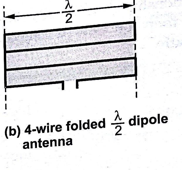
67 67

68 Fill in the blanks type of questions 1. The effective height of the antenna can be defined as the ratio of the to field 2. The condition for linear polarization is The condition for circular polarization is The condition for elliptical polarization is The fresenal zone is also called as

69 6. The Far field zone is also called as The antenna efficiency is the ratio of The formulae for the radiation resistance is The is the measure of the directivity of the antenna 10. The axial ratio is the ratio of Multiple choice questions 1. Radiation pattern is dimensional quantity [ ] a) Two b) three c) Single d) none is also called as 3-dB bandwidth [ ] a) FNBW b) HPBW c) Both a and b d) none 3. One steradian is equal to square degrees [ ] a) 360 b) 180 c) 3283 d) 41, is independent of distance [ ] a) Poynting vector b) radiation intensity c) Both a and b d) none 5. The minimum value of the directivity of an antenna is. [ ] a) Unity b) zero c) Infinite d) none 6. Directivity is inversely proportional to [ ] a) HPBW b) FNBW c) Beam area d) Beam width 7. Gain is always than directivity [ ] a) Greater b) lesser c) Equal to d) none 8. Directivity and Resolution are [ ] a) Different b) same c) Both a and b d) none 9. Effective aperture is always than Physical aperture. [ ] a) Higher b) lower c) Both a and b d) none Theorem can be applied to both circuit and field theories [ ] a) Equality of patterns b) Equality of impedance c) Equality of effective lengths d) Reciprocity theorem 11. Antenna temperature considers parameter into account [ ] a) Directivity b) gain c) Beam area d) beam efficiency 12. Radiation resistance of antenna is [ ] a) Physical resistance b) Virtual Resistance c) Both a and b d) none 69

70 Objective type of questions (Very short notes) 1. Define a Hertzian dipole? Oscillating dipole or Hertzian dipole is a current carrying conductor in which the charges at both the ends starts at oscillate. Its length is very small compared to λ. 1. What is radiation resistance of a half wave dipole? (Rr = 80 π 2 (dl/ λ) 2 ohms. Where Rr = Radiation resistance Dl = length of the current element λ = Wavelength. 2. List some applications of monopole antenna. It is used in compact communications system like, Hand phones Remote control etc., 3. What is radiation resistance? Radiation resistance is the amount of opposition offered by an antenna to radiate the energy to free space. It is the ratio between power radiated by an antenna to the square of rms current flow in that antenna. 4. Define Hertz antenna. It is a symmetrical dipole antenna in which the two ends are at equal potential relative to mid point whose length is equal to the half of the wavelength. 6. Define self- impedance Self -impedance of an antenna is defined as its input impedance with all other antennas are completely removed i.e away from it. 7. What is point source? It is the waves originate at a fictitious volumelessemitter source at the center of the observation circle. 8. What is mean by loop antenna? An antenna is a radio antenna consisting of a loop (or loops) of wire, tubing, or other electrical conductor with its ends connected to a balanced transmission line. 9. Define half wave dipole antenna 70

71 A dipole antenna is the simplest type of radio antenna, consisting of a conductive wire rod thatis half the length of the maximum wavelength the antenna is to generate. This wire rod is split in the middle, and the two sections are separated by an insulator. 10. What is meant by isotropic radiator? A isotropic radiator is a fictitious radiator and is defined as a radiator which radiates fields uniformly in all directions. It is also called as isotropic source or omni directional radiator or simply unipole. Analytical type questions 1. Derive the Expressions for and of radiated in a space by an alternating current element 2. Find out when the radiation resistance of the dipole antenna is 80π 2 3. Using Maxwell equations derive the Lorentz s gauge equation 4. Using Maxwell equations derive the retarded potential equation 5. Derive the expression for power radiated by antenna Essay type Questions <As per requirements> 1. Explain the concept o retarded potentials by using different approaches 2. Explain clearly about dipole, mono pole and tripole 3. Derive the expressions for magnetic field and electric field radiated by half wave dipole 4. Derive the expressions for magnetic field and electric field radiated by quarter wave dipole 5. Show that the directional pattern of an antenna as a when used as a receiving antenna is identical to that when used as transmitting antenna 6. Derive the equivalence of the impedance of the transmitting and receiving antennas Previous Questions (Asked by JNTUK from the concerned Unit) 71

72 1. State and prove the equality of the effective lengths of the transmitting and receiving antennas 2. Obtain the expressions for average power in terms of r.m.s current and write the radiation remittances of the half wave dipole 3. Obtain the expressions for average power in terms of r.m.s current and write the radiation remittances of the quarter wave dipole 4. Derive the expressions for electric field and magnetic field of the quarter wave dipole 5. Derive the expressions for electric field and magnetic field of the half wave dipole 6. Show that the directional pattern of the antenna as a receiving antenna is identical to that as transmitting antenna 4 Unit-wise course material 72

73 4.2 Unit III Antenna Arrays 2 element arrays different cases, Principle of Pattern Multiplication, N element Uniform Linear Arrays Broadside, Endfire Arrays, EFA with Increased Directivity, Derivation of their characteristics and comparison; Concept of Scanning Arrays. Directivity Electronics & Communication Engineering Relations (no derivations). Related Problems. Binomial Arrays, Effects of Uniform and Non-uniform Amplitude Distributions, Design Relations. Arrays with Parasitic Elements, Yagi-Uda Arrays, Folded Dipoles and their characteristics. Introduction The field radiated by a small linear antenna is not distributed uniformly in the case of a short dipole, the direction perpendicular to the axis of the antenna. As in maximum radiation takes place in the direction right angles to the axis of the dipole. But it decreases to minimum when the polar angle decreases. So, these non-uniform radiation characteristics may be used for many broadcast services. But such a characteristics are not preferred in point to point communication. In the point to point communication, it is desired to have most of the energy radiated in one particular direction. That means it is desired to have greater directivity in a desired direction particularly which is not possible with single dipole antenna. In general, antenna array is the radiating system in which several antennas are spaced properly so as to get greater field strength at a far distance from the radiating system by combining radiations at point from all the antennas in the system. In general, the total field produced by the antenna array at a far distance is the vector sum of the fields produced by the individual antennas of the array. The individual element is generally called element of an antenna array. The antenna array is said to linear if the elements of the antenna array are equally spaced along a straight line. The linear antenna array is said to be uniform linear array if all the elements are fed with a current of equal magnitude with progressive uniform phase shift along the line. 73

74 In general, the element in the antenna array is a -f dipole. The length of half wavelength dipole may not be equal to the electrical wavelength. If the variation of the electrical length from is within 5 % then it is assumed that the radiation properties of individual elements are not affected. As the antennas may be used in various configurations such as straight line, circle, rectangle etc., many configurations of antenna arrays are possible. But practically limited number of configurations is used extensively. Hence antenna array is a radiating system in contribute to obtain maximum field strength in the individual field strength in all other directions desired direction. Various Forms of Antenna Arrays Practically various forms of the antenna array are used as radiating systems. Some of the practically used forms are as follows. 1. Broadside Array 2. End fire Array 3. Collinear Array 4. Parasitic Array This form of the antenna array is one of the most important practical forms used in practice. The broadside array is the array of antennas in which all the elements are placed parallel to each other and the direction of maximum radiation is always perpendicular to the plane consisting elements. A typical arrangement of a Broadside array is as shown in the Figure. A broadside array consist number of identical antennas placed parallel to each other along a straight line. This straight line is perpendicular to the axis of individual antenna. It is known as axis of antenna array. Thus each element is perpendicular to the axis of antenna array. All the individual antennas are spaced equally along the axis of the antenna array. The spacing between any two elements is denoted by d. All the elements are fed with currents with equal magnitude and same phase. As the maximum point sources with equal amplitude and phase radiation is directed in broadside direction i.e. perpendicular to the line of axis of array, the radiation pattern for the broadside array is bidirectional. Thus we can define broadside array as the arrangement of 74

75 antennas in which maximum radiation is in the direction perpendicular to the axis of array and plane containing the elements of array. Now consider two isotropic point sources spaced equally with respect to the origin of the coordinate system as shown in the Fig Assume that the two point sources are with equal amplitude and phase. Figure - Broadside array of antennas 75

76 Broadside array with two isotropic point sources with equal amplitude and phase Consider that point P is far away from the origin. Let the distance of point P from origin be r. The wave radiated by radiator A 2 will reach point P as compared to that radiated by radiator A l. This is due to the path difference that the wave radiated by radiator A l has to travel extra distance. Hence the path difference is given by, Path difference = d cos ϕ This path difference can be expressed in terms of wave length as Path difference = cos ϕ From the optics the phase angle is 2π times the path difference. Hence the phase angle is given by Phase angle = ψ =2π (Path difference) Ψ = 2π 76

77 Ψ = d cosϕ Ψ = βdcosϕ End Fire Array The end fire array is very much similar to the broadside array from the point of view of arrangement. But the main difference is in the direction of maximum radiation. In broadside array, the direction of the maximum radiation is perpendicular to the axis of array; while in the end fire array, the direction of the maximum radiation is along the axis of array. End Fire Array Thus in the end fire array number of identical antennas are spaced equally along a line. All the antennas are fed individually with currents of equal magnitudes but their phases vary progressively along the line to get entire arrangement unidirectional finally. i.e. maximum radiation along the axis of array. Thus end fire array can be defined as an array with direction of maximum radiation coincides with the direction of the axis of array to get unidirectional radiation. Collinear Array As the name indicates, in the collinear array, the antennas are arranged co-axially i.e. the antennas are arranged end to end along a single line as shown in the Fig (a) and (b). 77

78 (a) Vertical (b) Horizontal Different Types of Collinear Array The individual elements in the collinear array are fed with currents equal in magnitude and phase. This condition is similar to the broadside array. In collinear array the direction of maximum radiation is perpendicular to the axis of array. So the radiation pattern of the collinear array and the broadside array is very much similar but the radiation pattern of the collinear array has circular symmetry with main lobe perpendicular everywhere to the principle axis. Thus the collinear array is also called omnidirectional array or broadcast array. The gain of the collinear array is maximum if the spacing between the elements is of the order of 0.3 λ to 0.5 λ. But this small spacing introduces constructional and feeding same. To derive different expressions following conditions can be applied to the antenna array Two point sources with currents of equal magnitudes and with same phase. Two point sources with currents of equal magnitude but with opposite phase. Two point sources with currents of unequal magnitudes and with opposite phase. 78

79 Two Point Sources with Currents Equal in Magnitude and Phase Consider two point sources A l and A 2 separated by distance d as shown in the Figure of two element array. Consider that both the point sources are supplied with currents equal in magnitude and phase. Consider point P far away from the array. Let the distance between point P and point sources A l and A 2 be r 1 and r 2 respectively. As these radial distances are extremely large as compared with the distance of separation between two point sources i.e. d, we can assume, r 1 = r 2 = r Two Element Array The radiation from the point source A 2 will reach earlier at point P than that from point source A l because of the path difference. The extra distance is travelled by the radiated wave from point source A l than that by the wave radiated from point source A 2. Hence path difference is given by, Path difference = d cos θ This path difference can be expressed in terms of wave length as Path difference = cos θ 79

80 From the optics the phase angle is 2π times the path difference. Hence the phase angle is given by Phase angle = ψ =2π (Path difference) Ψ = 2π Ψ = d cosϕ Ψ = βdcosϕ Above equation represents total field intensity at point P, due to two point sources having currents of same amplitude and phase. The total amplitude of the field at point P is 2E 0 while the phase shift is βd The array factor is the ratio of the magnitude of the resultant field to the magnitude of the maximum field. Therefore A.F. = But maximum field is = 2 The array factor represents the relative value of the field as a function of ϕ. It defines the radiation pattern in a plane containing the line of the array. Maxima Direction From above equation, the total field is maximum when cos is maximum. 80

81 As we know, the variation of cosine of a angle is ± 1. Hence the condition for maxima is given by, Let spacing between the two point sources be λ/2. Then we can write cos then we can say Minima direction Again from equation (4.4.9), total field strength is minimum when cos is minimum that is 0 as cosine angle has minimum value 0. Hence the condition for minima is given by, cos = 0 then we can say that Half power point directions When the power is half, the voltage or current is times the maximum value. Hence the condition for half power point is given by, Then by simplifying the above expression we will get The field pattern drawn with E T against ϕ for d = then the pattern is bidirectional as shown in the figure. The field pattern obtained is bidirectional and it is a figure of eight (8). If this pattern is rotated by 360 about axis, it will represent three dimensional 81

82 doughnut shaped space pattern. This is the simplest type of broadside array of two point sources and it is called Broadside couplet as two radiations of point sources are in phase. Field pattern for two point source with spacing d= d = and fed with currents equal in magnitude and phase Two Point Sources with Currents Equal in Magnitudes but Opposite in Phase Consider two point sources separated by distance d and supplied with currents equal magnitude but opposite in phase. For the above figure all the conditions are exactly same except the phase of the currents is opposite i.e With this condition, the total field at far point P is given by, E T = (-E l ) + (E 2 ) 82

83 Assuming equal magnitudes of currents, the fields at point P due to the point sources A l and A 2 can be written as, E l = E 0 E 2 = E 0 And substituting the values of E l and E 2 in the above equation we will get E T = E 0 + E 0 Finally we will get E T = j2e 0 sin( Now as the condition for two point sources with currents in phase and out of phase is exactly same, the phase angle can be written as previous case Phase angle = E T = j2e 0 sin Substituting value of phase angle in equation we get, E T = j2e 0 sin Maxima direction From the above equation, the total field is maximum when sin is maximum that is, Hence the condition for maxima is sin By taking the spacing between two isotropic point sources be equal to that is d = and β = in the above equation and simplifying we will get Φ max = 83

84 Minima direction Again from above equation total field strength is minimum when sin is minimum that is zero. Hence the condition is given by sin = 0 By taking the spacing between two isotropic point sources be equal to that is d = and β = in the above equation and simplifying we will get Φ min = -9 0 Half Power Point Direction When the power is half, the voltage or current is times the maximum value. Hence the condition for half power point is given by, By taking the spacing between two isotropic point sources be equal to that is d = and β = in the above equation and simplifying we will get Then by simplifying the above expression we will get As compared with the field pattern for two point sources with in-phase currents, the maxima have shifted by 90 along X-axis in case of out-phase currents in two point source array. Thus the maxima is along the axis of the array or along the line joining two point sources. In first case, we have obtained vertical figure of 8. Now in above case we have obtained horizontal figure of 8. AS the maximum field is along the line joining the two point sources, this is simple type of end fire array. 84

85 Field pattern for two point sources with spacing d = and fed with currents equal in magnitude but out of phase by Two Point Sources with Currents Unequal in Magnitudes and with any Phase If the two point sources are separated by distance d and supplied with currents which are different in magnitudes and with any phase difference say α. Consider that source 1 is assumed to be reference for phase and amplitude of the fields E 1 and E 2, which are due to source 1 and source 2 respectively at the distant point P. Let us assume that E 1 is greater than E 2 in magnitude as in diagram Now the total phase difference between the radiations by the two point sources at any far point is given by Ψ = cosθ+α 85

86 Vector Diagram of fields E 1 and E 2 where α is the phase angle with which current I 2 leads current I 1. Now if a then the condition is similar to the two point sources with currents equal in magnitude and phase. Similarly if α = 180, then the condition is similar to the two point source with currents equal in magnitude but opposite in phase. Assume value of phase difference a as 0 < α < 180. Then the resultant field at point P is given by, E T = E 1 + E 2 E T = E 1 + E 2 E T = E 1 (E 1 + Let = k note that E 2 > E 1, the value of k is less than unity. Moreover the value of k is given by 0 Then E T =E 1 [1+k(cosψ + jsinψ)] The magnitude of the resultant field at point P is given by The phase difference between two fields at the far point P is given by n Element Uniform Linear Arrays 86

87 At higher frequencies, for point to point communications it is necessary to have a pattern with single beam radiation. Such highly directive single beam pattern can be obtained by increasing the point sources in the arrow from 2 to n say. An array of n elements is said to be linear array if all the individual elements are spaced equally along a line. An array is said to be uniform array if the elements in the array are fed with currents with equal magnitudes and with uniform progressive phase shift along the line. Consider a general n element linear and uniform array with all the individual elements spaced equally at distance d from each other and all elements are fed with currents equal in magnitude and uniform progressive phase shift along line as shown in figure. Uniform, linear array of n elements The total resultant field at the distant point P is obtained by adding the fields due to n individual sources vectorically. Hence we can write, E T = E 0 + E E 0 E T = E 0 [ ] 87

88 Note that ψ =(βdcos(θ) + α) indicates the total phase difference of the fields from adjacent sources calculated at point P. Similarly α is the progressive phase shift between two adjacent point sources. The value of a may lie between 0 and 180. If α = 0, we get n element uniform li near broadside array. If α = 180, we get n element uniform linear-end-fire-array. Multiplying above equation by, we get, E T = E 0 [ ] Subtracting and the above two equations and simplifying we will get E T =E 0 Simplifying we will get E T =E 0 Then the magnitude of the resultant field is given by E T =E 0 The phase angle θ of the resultant field at point P is given by, = Array of n Elements with Equal Spacing and Currents Equal in Magnitude and Phase - Broadside Array Consider the 'n' number of identical radiators carry currents which are equal magnitude and in phase. The identical radiators are equispaced. Hence the maxim radiation occurs 88

89 in the directions normal to the line of array. Hence such an array known as Uniform broadside array. Consider a broadside array with n identical radiators as shown in figure. The electric field produced at point P due to an element A 0 is given by, E 0 = As the distance of separation d between any two array elements is very sai compared to the radial distances of point P from A 0, A 1,. A n-1, we can assume r 1, r 2, r n-1 are approximately same. Now the electric field produced at point P due to an element A 1 will differ in as r 0 and r 1 are not actually same. Hence the electric field due to A 1 is given by, E 1 = But E 1 = 89

90 E 1 =E 0 Exactly on the similar lines we can write the electric fieto the ld produced at point P due to an element A 2 is E 2 = E 2 = E 2 =E 1 By substituting E 1 the equation becomes Similarly E 2 =E 1 E n-1 =E 0 Then the total electric field at point P becomes E T = E 0 + E T = E 0 +E 1 + +E n-1 By writing the βdcosϕ =ψ then the above equation becomes E T = E 0 + Considering the series by s= 1+r+r 2 +r 3 +..r n-1 Where r = Multiplying the above equation on the both sides by r and simplifying we will get 90

91 By this series the ET becomes E T = E T = By simplifying we will get The exponential term in above equation represents the phase shift. Now considering magnitudes of the electric fields, we can write Properties of Broadside Array 1. Major lobe In case of broadside array, the field is maximum in the direction normal to the axis of the array. Thus the condition for the maximum field at point P is given by ψ = 0 i.e. βdcosϕ = 0 i.e. cosϕ = 0 i.e. ϕ = 90 0 or Thus ϕ = 90 and ϕ = 270 are called directions of principle maxima. 2. Magnitude of major lobe The maximum radiation occurs when ψ = 0. Hence we can write, 91

92 where, n is the number of elements in the array. Thus from equation, it is clear that, all the field components add up together to give total field which is 'n' times the individual field when ϕ = 90 or ϕ= Nulls The ratio of total electric field to an individual electric field is given by By making above equation to zero we can find the minima, but the above eq uation becomes zero then Now ψ = βdcosϕ Therefore N= number of elements in array d= Spacing between elements in meter λ = Wavelength in meter m= constant = 1,2, Subsidary maxima (or side lobes) 92

93 The directions of the subsidiary maxima or side lobes can be obtained if in above equation Hence sin( is not considered because if then sin ( =1 whch is the direction of principle maxima Hence we can skip value Thus, we can get Now ψ = βdcosθ By simplifying we can get The above equation represents the directions where certain radiation which is not maximum. Hence it represents directions of subsidary maxima or side lobes. 5. Beamwidth of major lobe The beamwidth is defined as the angle between first nulls. Alternatively beamwidth is the angle equal to twice the angle between first null and the major lobe maximum direction. Hence the beamwidth between first nulls is given by, 93

94 BWFN = 2*γ, where γ = 90-ϕ, where m= 1, 2, 3. And 90-γ = Taking the cosine angle on both sides cos(90-γ) = cos( If γ is very small, sinγ=γ, substituting in the above equation, we can get γ = But for the first null m=1 γ = BWFN = 2γ = But nd (n-1) d if n is very large. This nd indicates total length of aray in meter. This is denoted by L. BWFN = BWFN = degrees The Half Power beam width (HPBW) is given by HPBW = HPBW = degrees 94

95 6. Directivity The directivity is defined as Where the U 0 is the average radiation intensity and is given by U 0 = From the expression of ratio of magnitudes we can write, For the normalized condition Thus field from array is maximum in any direction 8 when w = 0. Hence normalized field pattern is given by, E Normalized = Hence the field is given by, E Normalized = Where ψ =βdcosθ The equationindicates array factor, hence we can write, the electric field due to n arrays as E = 95

96 Assuming d very small as compared to length of array, we can approximate Substituting the value of E in equation we get U 0 = Let z= and then simplifying we will get U 0 =- For large array, n is large hence nf3d is also very large (assuming tending to Hence of threwriting above equation. U 0 =- But so the equation becomes U 0 = the directivity is given by G Dmax = But U max = 1 at θ =90 0 and directivity we will get is G Dmax = L= (n-1)d, d nd if n is very large Then the directivity in terms of the total length array as 96

97 G Dmax = 2 ) Array of n Elements with Equal Spacing and Currents Equal in Magnitude but with Progressive Phase Shift - End Fire Array Consider n number of identical radiators supplied with equal current which are not in phase as shown in the figure. Assume that there is progressive phase lag of 13d radians in each radiator. End fire Array Consider that the current supplied to first element A 0 be I 0. Then the current supplied to A 1 is given by, I 1 = I 0 Similarly the current supplied to A 2 is given by, I 2 =I 1. = I 0 Thus the current supplied to the last element is given by, I n-1 = I 0 97

98 The electric field produced at point P, due to A 0 is given by, E 0 = The electric field produces at point P due to A 1 is given by E 1 = But E 1 = E 1 =E 0 Let E 1 =E 0 The electric field at point P due to A2 is given by Similarly E 2 =E 0 E n-1 =E 0 Then the total electric field at point P becomes E T = E 0 +E 1 + +E n-1 E T = E 0 + Considering the series by s= 1+r+r 2 +r 3 +..r n-1 Where r = 98

99 Multiplying the above equation on the both sides by r and simplifying we will get By this series the E T becomes E T = E T = By simplifying we will get the magnitude as Properties of End Fire Array 1. Major lobe For the end fire array where currents supplied to the antennas are but the phase changes progressively through array, the phase angle is ψ= βd (cos(θ-1)) i.e. cosθ =1 θ=0 0 Thus θ=0 0 indicates the direction of principle maxima. Also it indicates that maximum radiation is along the axis of array or line of array. 2. Magnitude of major lobe The maximum radiation occurs when ψ = 0. Hence we can write, 99

100 where, n is the number of elements in the array. Thus from equation, it is clear that, all the field components add up together to give total field which is 'n' times the individual field when θ = Nulls The ratio of total electric field to an individual electric field is given by By making above equation to zero we can find the minima, but the above equation becomes zero then nβd(cosθ-1)/2 = By simplifying we will get N= number of elements in array d= Spacing between elements in meter λ = Wavelength in meter m= constant = 1,2,

101 Then 4. Subsidary maxima (or side lobes) The directions of the subsidiary maxima or side lobes can be obtained if in above equation Hence sin( is not considered because if then sin ( =1 whch is the direction of principle maxima Hence we can skip value Thus, we can get, where m=1, 2, 3. By simplifying we can get The above equation represents the directions where certain radiation which is not maximum. Hence it represents directions of subsidary maxima or side lobes. 5. Beamwidth of major lobe The Beamwidth of the end fire array is greater than broad side array. 101

102 Beamwidth = 2*Angle between first nulls and maximum of the major lobe i.e. θ min If is very low, then we can write sin Using this property in above equation we will get ϕ min = But n=l i.e. length of the antenna array, so the equation can be written as ϕ min = BWFN = 2 ϕ min = BWFN = 2 ϕ min = *57.3 BWFN = degree 6. Directivity The directivity is defined as 102

103 But nd = L = Length of the array then Array of n Elements with Equal Spacing and Currents with Equal Amplitude and Progressive Phase Shift-End Fire Array with Increased Directivity The maximum radiation can be obtained along the axis of the uniform end fire array if the progressive phase shift a between the elements is given by, α = βd =-βd for maximum in θ =0 0 direction = +βd for maximum in θ=180 0 direction It is found that the field produced in the direction θ = 0 is maximum; but the directivity is not maximum. In many applications it is necessary to have the maximum possible directivity of the linear array. In 1938, Hansen and Woodyard proposed certain conditions for the end fire case which are helpful in enhancing the directivity without altering other characteristics of the end fire array. These conditions are popularly known as Hansen-Woodyard conditions for End Fire Radiation. According To Hansen-Woodyard conditions, the phase-shift between closely spaced radiators of a very long array should be α = (βd+2.94/n) -(βd+ ) for maximum in θ =0 0 direction and α = (βd+2.94/n) +(βd+ ) for maximum in θ =180 0 direction 103

104 Note that with above conditions also maximum possible directivity cannot be achieved. That means the maximum may not even occur at ϕ=0 and ϕ=180, its magnitude maximum may not be unit and even side lobe level may not be db. Basically the maxima level and side lobe level, both depend on 'n' i.e. number of elements in the array. The enhanced directivity due to Hansen-Woodyard conditions can be realized by using above equation along with assumptions for values given as below. 1) For maximum radiation along θ = 0 0 and ii) For maximum radiation along θ = 180 and Even though above equations represent conditions obtained from equation of first set only, the precaution must be taken to fulfill the condition = π for each array. In general, for an array of n elements, the condition = π It can be satisfied by using equation of first set for θ = 0 and θ =180 by selecting the spacing between two elements as, d = 104

105 If the number of elements is considerably large, then we can write, d = Hence for large uniform array, the Hansen-Woodyard conditons illustrate enhanced directivity if the spacing between the two adjacent elements is approximately λ/ 4 Consider n element array. The array factor of the n-element array is given by, (AF) n = But ψ = βdcosθ +α. Putting in above equation,we can get (AF) n = For smaller values of ψ the above expression becomes (AF) n = (AF) n = Let the progressive phase shift be α = -pd, where p is constant. Then above equation becomes (AF) n = (AF) n = 105

106 Let Hence the above equation becomes (AF) n = Let then the above equation becomes (AF) n = The radiation intensity U(ϕ) = = Atθ=0 0, the radiation intensity is given by U(ϕ=0 0 ) = = Dividing above two equations and let z=q(β-p) U(θ) n = 1 The directivity of the array factor is given by, D 0 = = = The average radiation intensity is given by By simplifying we can get U 0 = where v = q(β-p) 106

107 When the g(v) is plotted against v, its minimum value appears when v= q(β-p)= =-1.47 α = -pd =- The above equation gives the condition for the end fire array with enhanced directivity based on Hansen woodyard conditions The variation g(v) as a function of v is as figure below. variation g(v) as a function of v The field pattern for 4 element end fire array with equal amplitude and spacing for increased directivity is as drawn below 107

108 field pattern for 4 element end fire array with equal amplitude and spacing for increased directivity Directivity of end fire array with increased directivity For end fire array with increased directivity and maximum radiation in ϕ=00 direction, the radiation on intensity for small spacing between elements (d<<λ) is given U 0 = By simplifying we can get U 0 = Pattern Multiplication Method And the directivity becomes D =1.789(4(L/λ)) where L= (n-1)d = nd The simple method of obtaining the patterns of the arrays. This method is known as pattern multiplication method. This method is a very useful in the design of arrays because it makes possible to draw the patterns of complicated arrays rapidly, almost by inspection. To illustrate this method, consider 4 element array of equispaced identical 108

109 antennas as shown in the figure. Let the spacing between two units be d = λ/2. Also assume that all the elements are supplied with equal magnitude currents which are in phase. As the point P at which the resultant field has to be obtained is far away, we can assume the radiation from the antenna in the form of parallel lines. The radiation pattern of the antennas (1) and (2) treated to be operating as a single unit is as shown in the Figure (a). Similarly the radiation pattern of the antennas (3) and (4), spaced d = λ/2 distance apart and fed with equal current in phase, treated to be operated as single unit is again as shown in the Figures(a). Now instead of considering two separate elements (1) and (2), we can replace it by a single antenna located at a point midway between them as shown in the figure(c). Now Similarly replacing antennas (3) and (4) by single antenna having same pattern as shown in the Figure (c). Now both the antennas have bi direction pattern i.e. figure eight pattern spaced distance λ apart from each other, fed with equal currents in phase is as shown in the Figure (b). Now the resultant radiation pattern of four element array can be obtained as the multiplication of pattern as shown in the Figure (d). Note that this multiplication is polar graphical multiplication for different values of ϕ. (a) Radiation Pattern of two antennas spaced at distance and fed with equal currents in phase 109

110 (b) Radiation Pattern of two antennas spaced at distance and fed with equal currents in phase (c) Array of 4 identical elements. Replacement of array by two single antennas placed at distance λ (d) Multiplication of pattern Binomial Array In case of uniform linear array, to increase the directivity, the array length has to be increased. But when the array length increases, the secondary or side lobes appear in the pattern. In some of the special applications, it is desired to have single main lobe with no minor lobes. That means the minor lobes should be eliminated completely or reduced to minimum level as compared to main lobe. To achieve such pattern, the array is arranged in such a way that the broadside array radiate more strongly at the centre than that from edges. Let us consider array of the 110

111 two identical in-phase point sources spaced λ/2 apart. Then the far-field pattern is given by E = cos( In case of uniform 4-element array, the resultant pattern shows four side lobes. The secondary lobes appear in the resultant pattern, because the elements producing the group pattern have a spacing greater than one-half eave length. So 4 element array, the elements producing pattern are spaced a full wave length apart. So if we reduce the spacing between two elements to one half wavelength then only the primary lobes are obtained. Field pattern for two point sources with equal amplitude in-phase current (a) Arrangement of 4-elements with λ/2 spacing 111

112 (b) Pattern for 2-element array and 4-element array The two element arrays are spaced 2 distance apart from each other. Such array produces increased radiation pattern with no secondary lobes. Here antenna 2 and 3 coincide at the centre as shown in the Figure (a). Hence it can be replaced by a single element carrying double current compared with other elements. Thus as shown in the Figure (b), the resultant array consists three elements with current ratio 1 : 2 : 1. The same concept can be extended further by considering three element array as a unit and with a second similar three element array spaced half-wave length from it. This results in 4-element array as shown in the Fig In this array, the current ratio is given by 1 : 3 : 3 : 1. Four element Array If we continue this process, we can obtain the pattern with arbitrarily large directivity without minor lobes. But it is necessary to adjust the amplitudes of the currents. In the array corresponding to the coefficient of the binomial series. This concept was first proposed by John Stone in As the secondary or side lobes in the linear broadside arrays can be eliminated totally when the amplitude of the currents in the radiating sources are proportional to the coefficients of the binomial series. In general the pattern for the binomial array is given by E =cos n-1 [π/2cosθ] n= number of sources in the array 112

113 Phased Arrays or Scanning Arrays In case of the broadside array and the end fire array, the maximum radiation can be obtained by adjusting the phase excitation between elements in the direction normal and along the axis of array respectively. That means in other words elements of antenna array can be phased in particular way. So we can obtain an array which gives maximum radiation in any direction by controlling phase excitation in each element. Such an array is commonly called phased array. The array in which the phase and the amplitude of most of the elements is variable, provided that the direction of maximum radiation (beam direction) and pattern shape along with the side lobes is controlled, is called as phased array. Suppose the array gives maximum radiation in the direction ϕ=ϕ 0 then the phase shift that must be controlled can be obtained as follows. Ψ =kdcosθ+α At θ=θ 0 the value of ψ is zero. Then α = -kd cosθ 0 Thus from equation, it is clear that the maximum radiation can be achieved in any direction if the progressive phase difference between the elements is controlled. The electronic phased array operates on the same principle. Consider a three element array, the element of array is considered as λ/2 dipole. All the cables used are of same length. All the three cables are brought together at common feed point. Here mechanical switches are used. Such switch is installed one at each antenna and one at a common feed point. All the switches are ganged together. Thus by operating switch, the beam can be shifted to any phase shift. 113

114 To make operation reliable and simple, the ganged mechanical switch is replaced by PIN dipole which acts as electronic switch. But for precision in results, the number of cables should be minimized. Phased array with mechanical switches at elements and feed point In many applications phase shifter is used instead of controlling phase by switching cables. It can be achieved by using ferrite device. The conducting wires are wrapped around the phase shifter. The current flowing through these wires controls the magnetic field within ferrite and then the magnetic field in the ferrite controls the phase shift. The phased array for specialized functional utility are recognized by different names such as frequency scanning array, retro array and adoptive array. The array in which the phase change is controlled by varying the frequency is called frequency scanning array. This is to be the simplest phased array as at each element separate phase control is not necessary. Each element of the scanning array is fed by a transmission line via directional coupler. Note that the directional couplers are fixed in position, while the beam scanning is done with a frequency change. To avoid reflections and to obtain pure form of the travelling wave, the transmission line is properly terminated of the load. The main advantage of the 114

115 frequency scanning array is that there are no moving parts and no switches and phase shifters are required. The array which automatically reflects an incoming signal back to the source is called retro array. It acts as a retro reflector similar to the passive square corner reflector. That means the wave incident on the array is received and transmitted back in the same direction. In other words, each element of the retro array reradiates signal which is actually the conjugate of the received one. Simplest form of the retro array is the Van Atta array as shown in the Figure in which 8 identical λ/2 dipole elements are used, with pairs formed between elements 1 and 8, 2 and 7, 3 and 6, 4 and 5 using cables of equal length. If the wave arrives at angle i say then it gets transmitted in the same direction. Frequency scanning line fed phased array Vanatta retro array 115

116 An array which automatically turn the maximum beam in the desired direction while turn the null in the undesired direction is called adoptive array. The adoptive array adjusts itself in the desired direction with awareness of its environment. In modern adoptive arrays, the output of each element in the array is sampled, digitized and then processed using computers. Such arrays are commonly called smart antennas. Effect of Uniform and Non-uniform Amplitude Distributions In the synthesis of antenna, it is often required to have narrowest main lobe for a given level of the side lobes. In other words, we can say that while designing antenna array it is often required to determine the current ratios resulting the smallest side lobe level for a specified beamwidth of the principal lobe. But these two characteristics of the antenna are related to each other, so any improvement in any one characteristic deteriorates the other one. Prof. C.L. Dolph suggested that for a linear in phase broadside arrays, for a specified side lobe level it is possible to minimize the beam width of main lobe and vice versa. The improvement in the above antenna characteristics proposed by Prof. C.L. Dolph was based on Tcliebyscheff polynomials. Thus according to him, if the beamwidth between first nulls is specified, then the side lobe level can be minimised. The current distribution that produce such a pattern is called Dolph-Tchebyscheff distribution or simply Tchebyscheff distribution. Thus the Tchebyscheft distribution provides a compromise between two conflicting properties. Such a value is considered to be an optimum condition. The antenna arrays based on the Dolph-Tchebyscheff distribution are called Dolph Tchebyscheff arrays which specified side lobe level and vice versa. The Tchebyscheff distribution proposed by Prof. C.L. Dolph is based on Tchebyscheff polynomials. The alternative spelling to the Russian name Tchebyscheft is only Chebyshev and thus the Dolph-Tchebyscheff arrays are simply called Chebyshev arrays. 116

117 According to Prof. C.L.Dolph, the current distribution is optimum provided that distance between two successive array elements d is less than or equal to λ/2. According to his approach, it is practically very difficult to reduce side lobe level without sacrificing the antenna performance in some other respect such as beamwidth, gain or directivity. With the help of Tchebyscheff distribution, it is possible practically to design an array with high gain and narrow beamwidth for the side lobe levels upto db in UHF and VHF bands. Note that 20 db level is considered to be good and 30 db to be excellent. But it practically very difficult to 40 db level. Fundamentals of Tchebyscheff Polynomials The Tchebyscheff polynomial with variable x is denoted by Tm (x). The Tchebyscheff polynomial is defined by equations given by, T m (x) = cos(m -1<x <1 T m (x) = cosh(m >1 Here m is integer constant with range from 0 to. The Tchebyscheff polynomials for different values of m. If m=0 T 0 (x) =1 If m=1 T 1 (x) =x If m=2 T 2 (x) = If m=3 T 3 (x) = 117

118 If m=4 T 4 (x) =8 If m=5 T 5 (x) = 16 If m=6 T 6 (x) = 32 The degree of Tchebyscheff polynomial is same as the value of m. The value of m can be either even or odd. The characteristics of Tchebyscheff polynomials for even and odd values of m are as shown in the figures respectively. From the characteristics of the Tchebyscheff polynomial following properties can be obtained. All the polynomials oscillate between the values - 1 and 1. In the region < 1, the m th order Tchebyscheff polynomial crosses the m-times. In the region > 1, the Tchebyscheff polynomial goes on increasing without any control. The rate at which the polynomial extends is given by x m. 118

119 Tchebyscheff polynomials for even and odd values of m So from the Fig , (a) and (b), when x is varied from any arbitrary point say a up to specific value x o and then varied back to a, then the polynomial T m (x) traces a pattern which includes, i) One major lobe, ii) Many side lobes, iii) The secondary minor lobes of same amplitude equal to unity. (These secondary minor lobes are below the main lobe by ratio 1/r which can be selected as per requirement by suitably selecting x 0 ). iv) Ideal lobes arising in the region x < 1, v) The main lobe extending far in the region x > 1. The above two figures are called optimum pattern as all the side lobe levels are of same amplitude. 119

120 The nulls of the Tchebyscheff pattern are given by roots of the m th degree Tchebyscheff polynomial as follows. Consider m th order Tchebyscheff polynomial given by Tm (x) = cos (mcos -l x) = cos mδ, where Then the nulls are given by the roots, cos mδ =0 Then δ = (2k-1) π/2m where k=1,2,3 Example 1:For two element array consisting identical radiators carrying equal currents in phase, obtain positions of maxima and minima of the radiation pattern if the distance of separation d = λ. Dipoles with Parasitic Elements Let I 1 be current in the driven element D. Similarly 12 be the current induced in the parasitic element P. The relation between voltages and currents can be written on the basis of circuit theory as, V 1 = Z 11 I 1 + Z 12 I 2 0 = Z 21 I 1 + Z 22 I 2 Note that as parasitic element P is not excited, the applied voltage V 2 is written zero. V 1 is the applied voltage to the driven element D. The impedances Z 11 and are the self-impedances of the driven element D and the parasitic element P. The impedances Z 12 and Z 21 is the mutual impedance between the two elements such that, Z 12 = Z 21 =Z M 120

121 Array in free space with one parasitic element and one driven λ/2 dipole element The current The resistance is given by The gain in field intensity as a function of θ is 121