Protocols and Criteria for Acoustic Emission Monitoring of Fracture-Critical Steel Bridges

Transcription

1 Protocols and Criteria for Acoustic Emission Monitoring of Fracture-Critical Steel Bridges A THESIS SUBMITTED TO THE FACULTY OF THE UNIVERSITY OF MINNESOTA BY Anton Stephen Tillmann IN PARTIAL FULFILLMENT OF THE REQUIREMENTS FOR THE DEGREE OF MASTER OF SCIENCE Adviser: Dr. Arturo Schultz June 2015

2 Anton Tillmann 2015

3 ACKNOWLEDGMENTS This work was supported by the Minnesota Department of Transportation, the Federal Highway Administration s Dwight David Eisenhower Transportation Fellowship, the Beavers Heavy Construction Fellowship, and the William H. Burgum Endowed Fellowship. The authors thank Paul Bergson of the Department of Civil, Environmental, and Geo- Engineering at the University of Minnesota, as well as fellow students Alireza Nojavan, Jacob Robole, Andrew Morgan, and Sam Konieczny for their assistance in the maintenance of the bridge monitoring equipment. The authors would also like to thank Daniel Morton, Alexandria Lee-Norris, and David Thompson who installed the equipment, and performed analyses and tests that were vital to progress of this research. i

4 I dedicate this work to the Master of Science Molly Krieser. Her presence in my life kept me on the path to achieving success. ii

5 ABSTRACT With bridge infrastructure in Minnesota aging, advancing techniques for ensuring bridge safety is a fundamental goal of the Minnesota Department of Transportation (MnDOT). Developing health monitoring systems for fracture-critical bridges is an essential objective in meeting the stated goal. This report documents the implementation of two, 16-sensor, acoustic emission monitoring systems in one of the tie girders of the Cedar Avenue Bridge, which is a fracture-critical tied arch bridge spanning the Minnesota River between Bloomington and Eagan, MN. The goal of the project is to develop a process for using acoustic emission technology to monitor one of the girders of the bridge while continuously collecting data from the monitoring systems. Given the cost of acoustic emission sensing equipment, an approach was adopted to space the sensors as widely as possible. Fracture tests were conducted on a specimen acoustically connected to the bridge to simulate fracture in a bridge member. Sets of criteria were developed to differentiate between acoustic emission data collected during fracture and ambient bridge (i.e. AE noise) data. The sets of criteria were applied to fracture test data and AE noise data to determine the validity of the criteria. For each criteria set, a period of Cedar Avenue Bridge monitoring data was analyzed. The results of the analysis of each period showed that the criteria could differentiate between the bridge AE noise data and the fracture data. The AE noise data never met all of the criteria in the set, whereas all criteria were met during each of the applicable fracture tests. iii

6 TABLE OF CONTENTS List of Figures... vii List of Tables... x Chapter 1 Introduction... 1 Chapter 2 Background, Scope, and Objective Background Scope Objective... 4 Chapter 3 Literature Review Acoustic Emission Testing in Laboratory Settings Acoustic Emission Monitoring of Infrastructure... 8 Chapter 4 Acoustic Emission Backgroud Acoustic Emission Sources Acoustic Emission Wave Propagation Wave Propagation Modes Wave Attenuation Acoustic Emission Monitoring Acoustic Emission Parameters Characteristics of Acoustic Emission from Fracture Chapter 5 Cedar Avenue Bridge Monitoring Methodology System Overview System Installation System Geometry System Power iv

7 5.5 Sensor Selection Sensor Calibration Wave Velocity Calibration Wave Attenuation Calibration System Settings Chapter 6 Acoustic Emission Acquisition in Fracture Beam Test Overview Notched Beam Fracture Test Summary Cedar Avenue Bridge Notched Beam Test Experimental Setup Beam Specimen Fabrication Connection Sensor Locations Power Solution Data Collection Laboratory Notched Beam Fracture Test Fracture Acoustic Emission Results and Discussion Chapter 7 - Collection of Acoustic Emission Data in the Cedar Avenue Bridge Bridge Data Collection Summary South System Data Collection North System Data Collection Solar Panel Power Source Chapter 8 - Fracture Criteria Development Development of Fracture Criteria First Fracture Criterion Set Second Fracture Criterion Set v

8 8.4 Third Fracture Criterion Set Chapter 9 Acoustic Emission Analysis of Cedar Avenue Bridge Data Data Analysis Summary First Bridge AE Data Set Second Data Set Third Data Set Chapter 10 Effectiveness of FRACTURE CRITERIA Definition of Effectiveness Effectiveness of Fracture Criterion Sets in Identifying Fracture Effectiveness of Fracture Criterion Sets in Rejecting Non-Fracture AE Data Discussion Chapter 11 - Summary, Conclusions, and recommendations Summary Conclusions Recommendations References Appendix A: Fracture Beam Test Results Appendix B: Notched Beam Fracture Test Amplitude Filters Appendix C: Velocity Calibration Results Appendix D: Troubleshooting and Maintenance Timeline Appendix E: Criteria Exceedances of the Third Criteria Set North System Appendix F: Criteria ExceedAnces of the Third Criteria Set South System vi

9 LIST OF FIGURES Figure 4.1: Lamb Waves: Left - Symmetric Mode, Right - Antisymmetric Mode Figure 4.2: Rayleigh Waves Figure 4.3: Idealized voltage wave and selected parameters (Pollock, 2003) Figure 4.4: Timing parameters used to define an individual hit Figure 5.1: Connection spacing and naming Figure 5.2: North and South System sensor positions and numbering Figure 5.3: Walking bridge adjacent to monitored tie girder photo Figure 5.4: Walking bridge adjacent to monitored tie girder plan view Figure 5.5: Power Supply Circuit (Physical Acoustics Corporation, 2010) Figure 5.6: Frequency response of R15l-AST ( MISTRAS Products and Systems Division, 2010) Figure 5.7: Obstructions between sensors Figure 6.1: Notched beam specimen profile for (a) BTN1/BTS1, (b) BTN2/BTS2 (All dimensions in inches) Figure 6.2: Field setup for notched beam test Figure 6.3: Sensor locations for (a) BTS1, (b) BTN Figure 6.4: Sensor locations for (a) BTS2, (b) BTN Figure 6.5: Hand pump connected to the jack (just out of view to the top of picture) Figure 6.6: Fracture Test Results Key Figure 7.1: South system data collection efficiency Figure 7.2: North system data collection efficiency Figure 9.1: Cumulative number of hits versus time for the first data set (a) Low activity day; (b) High activity day; (c) Anomalous day Figure 9.2: Number of hits versus frequency centroid for the first data set (a) Low activity day; (b) High activity day; (c) Anomalous day vii

10 Figure 9.3: Duration versus amplitude for the first data set (a) Low activity day; (b) High activity day; (c) Anomalous day Figure 9.4: Maximum absolute energy versus amplitude for the first data set (a) Low activity day; (b) High activity day; (c) Anomalous day Figure 9.5: Cumulative number hits versus time for the second data set in the north system (a) Low activity day; (b) High activity day; (c) Anomalous day Figure 9.6: Cumulative number of hits versus time for the second data set in the south system (a) Low activity day; (b) High activity day Figure 9.7: Number of hits versus frequency centroid for the second data set in the north system (a) Low activity day; (b) High activity day; (c) Anomalous day Figure 9.8: Number of hits versus frequency centroid for the second data set in the south system (a) Low activity day; (b) High activity day; Figure 9.9: Duration versus amplitude for the second data set in the north system (a) Low activity day; (b) High activity day; (c) Anomalous day Figure 9.10: Duration versus amplitude for the second data set in the south system (a) Low activity day; (b) High activity day Figure 9.11: Absolute energy rate versus time for the second data set in the north system: (a) Low activity day; (b) High activity day; (c) Anomalous day Figure 9.12: Absolute energy rate versus time for the second data set in the south system (a) Low activity day; (b) High activity day Figure 9.13: Count rate versus time for third data set in north system (a) Low activity day; (b) High activity day; (c) Anomalous day Figure 9.14: Count rate versus time for third data set in south system (a) Low activity day; (b) High activity day Figure 9.15: Time versus event location for third data set using the third fracture criterion set in the north system showing source amplitudes greater than 80dB (a) Low activity day; (b) High activity day; (c) Anomalous day Figure 9.16:Time versus event location for the third data set using the third fracture criterion set in the south system showing source amplitudes greater than 80dB (a) Low activity day; (b) High activity day Figure 9.17: Time versus event location for the third data set in the north system showing all events (a) Low activity day; (b) High activity day; (c) Anomalous day viii

11 Figure 9.18: Time versus event location for the third data set in the south system showing all events Figure 10.1: Fracture effectiveness during fracture beam tests Figure 10.2: Non-AE Signal Rejection Effectiveness from Bridge Data Set ix

12 LIST OF TABLES Table 5.1: Acoustic Emission Equipment from Mistras Group Inc Table 5.2: Average velocities between sensors Table 5.3: Attenuation pencil break test results Table 5.4: SH-II acquisition settings Table 6.1: Notched Beam Fracture Test Summary Table 6.2: Bridge and Notched Beam Steel Properties Table 6.3: Laboratory Fracture Test Results Table 6.4: North System Bridge Fracture Test Results Table 6.5: South System Bridge Fracture Test Results Table 6.6: Number of hits with duration > 30ms and amplitude > 90dB for each test.. 48 Table 7.1: Timeline of AE data records for the South System Table 7.2: Timeline of AE data records for the North System Table 8.1: First Fracture Criterion Set Table 8.2: First Criterion Set Exceedances Table 8.3: Second Fracture Criterion Set Table 8.4: Second Criterion Set Exceedances Table 8.5: Third Fracture Criterion Set Table 8.6: Third Criterion Set Exceedances Table 9.1: Frequency of exceedance for individual criteria using the first fracture criterion set and the first data set Table 9.2: Number of days a given number of criteria are exceeded using the first fracture criterion set and the first data set Table 9.3: Frequency of Exceedance for Individual Criteria using the Second Fracture Criterion Set and the Second Data Set in the Nouth System x

13 Table 9.4: Frequency of Exceedance for Individual Criteria using the Second Fracture Criterion Set and the Second Data Set in the South System Table 9.5: Number of Days a Given Number of Criteria were Exceeded using the Second Fracture Criterion Set and the Second Data Set in the North System Table 9.6: Number of Days a Given Number of Criteria were Exceeded using the Second Fracture Criterion Set and the Second Data Set in the South System Table 9.7: Frequency of Exceedance for Individual Criteria using the Third Fracture Criterion Set and the Third Data Set in the North System Table 9.8: Frequency of Exceedance for Individual Criteria using the Third Fracture Criterion Set and the Third Data Set in the South System Table 9.9: Number of Days a Given Number of Criteria were Exceeded using the Third Fracture Criterion Set and the Third Data Set in the North System Table 9.10: Number of Days a Given Number of Criteria were Exceeded using the Third Fracture Criterion Set and the Third Data Set in the South System Table 10.1: First Criterion Set Effectiveness to Identify Fracture Table 10.2: Second Criterion Set Effectiveness to Identify Fracture Table 10.3: Third Criterion Set Effectiveness to Identify Fracture Table 10.4: Non-AE Signal Rejection Effectiveness for First Criterion in South System Table 10.5: Non-AE Signal Rejection Effectiveness for Second Criterion Set in North System Table 10.6: Non-AE Signal Rejection Effectiveness for Second Criterion Set in South System Table 10.7: Non-AE Signal Rejection Effectiveness for Third Criterion Set in North System Table 10.8: Non-AE Signal Rejection Effectiveness for Third Criterion Set in South System xi

14 CHAPTER 1 INTRODUCTION This report documents the development of an advanced warning system that will be used to monitor fracture critical steel bridges. An advanced warning system offers the potential to detect initiation and propagation of fracture in bridges, and if so, proper steps can be taken to alleviate the structural distress before further damage is sustained. The need to monitor fracture critical bridges arises due to the concern over a bridge s inability to support itself after key members have failed. Fracture critical bridges are not inherently unsafe; however, more care should be taken while inspecting these bridges because fracture in a key member can undermine the capacity of the bridge if the crack is allowed to propagate. The tied arch steel bridge that carries Minnesota State Highway 77 over the Minnesota River was selected for this project. This bridge is known as the Cedar Avenue Bridge (MnDOT #9600N). The advanced warning system was chosen to consist of commercially available monitoring equipment that detects the acoustic emission phenomenon as a structure is undergoing fracture. The purpose of choosing to monitor the Cedar Avenue Bridge is not because the bridge is thought to be unsafe or susceptible to fatigue cracking. The Cedar Avenue Bridge has not experienced any known cracking in its lifetime. The bridge was chosen to serve as a platform on which to develop, implement, and test the monitoring technology. This report documents the collection of data to insure the adequate operation of the system and the development of data analysis procedures for use on data collected from the Cedar Avenue Bridge. This report contains 11 chapters and 6 appendices. Chapter 2 provides the summary of previous phases of the project, and the scope and objective of this phase of the project. Chapter 3 provides an overview of previous experiments that have taken place in the field of acoustic emission monitoring. Chapter 4 gives a background of acoustic emission technology and the theory behind the creation and collection of AE waves. Chapter 5 describes the methodology being used in this monitoring project. Chapter 6 describes the tests conducted to produce and collect acoustic emission waves from a fracture event. Chapter 7 outlines the monitoring timeline and the data collection process. Chapter 8 1

15 describes how the different fracture criterion sets were developed. Chapter 9 describes the evaluation of the bridge AE data. Chapter 10 consists of a discussion of the test results and data analysis. Chapter 11 concludes the report with a summary and closing comments. 2

16 CHAPTER 2 BACKGROUND, SCOPE, AND OBJECTIVE 2.1 Background This report details the work done in the third and final phase of the Cedar Avenue Bridge Acoustic Emission Monitoring Project. During the first phase of the project (Schultz & Thompson, 2010), the monitoring technology of acoustic emission (AE) was selected for monitoring the Cedar Avenue Bridge. AE technology was selected for the project because it was best suited to monitor fatigue cracking and fracture of welds allowing it to provide advanced warning for structural damage in steel bridges. The Cedar Avenue Bridge was selected to be monitored because it is a major fracture critical steel bridge and an important artery in the transportation network. The first phase included finite element analysis of the Cedar Avenue Bridge and modeling of local regions of high stress. The results of the finite element analysis were used to make the decision to monitor a large region of the bridge rather than to focus on localized regions susceptible to fatigue as has been done previously with AE (Hopwood II & Prine, 1987). The decision to monitor a large region of the bridge was made because there are numerous points along the bridge that may be susceptible to fracture. During the second phase of the project, the installation of the first (south) system took place. The sensors where installed at 10 ft. spacing and the sensor array was centered about the midspan of the bridge. This sensor distribution was chosen because it allowed for many highly stressed connections to be monitored. The second phase also included the calibration of the AE system to the Cedar Avenue Bridge, which included pencil break tests to determine the attenuation and wave velocity between the sensor locations. The sensor array remained in this location while being set to continuously collect data until May 2013 when a second, identical AE system was installed in the north portion of the bridge, and the original (south) system was moved to the southern one-half of the bridge. Before installation, the north system was used for a series of laboratory experiments, during which, a steel beam was fractured and the resulting AE data was collected. The data collected during these laboratory tests would become the basis for 3

17 developing criteria to be used in the Cedar Avenue Bridge capable of differentiating between fracture AE data and bridge AE data produced by non-fracture sources. 2.2 Scope This phase of the project consisted of (1) the collection of AE data produced by the bridge, (2) the creation of data evaluation metrics, and (3) the evaluation of the bridge AE data. Data from the bridge was collected by downloading data stored on the system s data storage website, and during times when the cellular connection was unavailable, data was directly downloaded from the system s computer inside the bridge girder. Data evaluation metrics where created in the form of a criterion set based on fracture beam tests. The criterion set was then used to evaluate the AE bridge data to determine if any fracture events had been collected by the bridge AE system. Based on research performed during this phase of the project, recommendations are made for advancing the use of AE technology in bridge health monitoring. 2.3 Objective The overall objective of the project was to develop a system that is able to detect the onset of crack initiation and crack propagation in the Cedar Avenue Bridge. This objective was to be achieved through the use of an Acoustic Emission monitoring system. The overall objective was further subdivided into project goals to help achieve the primary objective. The goals of this project were (1) to determine the characteristics of an AE wave created from a fracture event, (2) to collect bridge AE data to determine the characteristics of AE waves that are, for the vast majority, not from fracture, and (3) to develop a procedure for monitoring and evaluating bridge AE data. By achieving these goals, the project will have advanced AE technology towards the realm of monitoring large portions of bridges or entire bridges. 4

18 CHAPTER 3 LITERATURE REVIEW The recognition of the acoustic emission (AE) phenomenon dates back to the late 19 th and early 20 th century when scientists correlated deformations in material with audible noises. A notable example of this is when Albert Portevin and Francois Le Chatelier observed AE emissions from a stressed Aluminum-Copper-Manganese alloy in their work which lead to the development of the PLC (Portevin Le Chatelier) effect, which is the inconsistent behavior of a metal being stressed beyond its yield point (Yilmaz, 2011). The AE phenomenon itself was not specifically studied until the 1950 s when Joseph Kaiser conducted research on the subject. Kaiser studied the acoustic emissions released when loading polycrystalline metal specimen. He discovered that no further emissions would be released until the previous highest stress in the material was exceeded (Kaiser, 1950). This effect now bears Joseph s name and is known as the Kaiser Effect. AE evolved as a non-destructive testing (NDT) method as computer processing became readily available. The technology was first used in industry for weld quality inspection. During and after the welding process, hydrogen escaping the weld may cause it to crack. In 1969 W.D Jolly found that acoustic emission technology was capable in detecting defaults in welds by measuring the emissions produced by crack defects (Jolly, 1969). After AE proved its ability to detect small amounts of cracking in welds it began to gain interest in the infrastructure and tank vessel inspection communities and has become a very popular method of NDT today. Today acoustic emission testing is used in a wide array of laboratory experimentation where strength of material is being tested. This literature review provides an overview to work that has been instrumental in the development of this thesis. 3.1 Acoustic Emission Testing in Laboratory Settings Barsoum, Suleman, Karcak, and Hill (2009) performed an experiment using acoustic emission (AE) sensors to monitor fatigue cracking in an axial loaded notched beam. The 5

19 data collected during various stages where used to predict the fatigue life of the beam. The experimental setup included a notched beam specimen of 305mm with the acoustic emission sensors placed on either side of the notch. Ambient noise measurements were taken before applying stress to the beam in order to characterize ambient noise data produced by the fatigue machine and other noise sources. It was found that a vast majority of the hits from noise had an average frequency of between 1kHz and 30kHz, but there were also discrete values of higher frequencies with a fair number of hits. This low frequency characteristic was used to filter out AE noise once the fatigue loading was started. It was found that AE noise hits fall in an isolated region on a duration vs. counts plot, and for the most part can be distinguished from actual plastic deformation hits. Three different types of notched beams were tested under fatigue loading. A thin beam designed to fracture under plain stress, a thick beam designed to fracture under plane strain, and a medium size that was designed to fracture under a mixed mode. The results of the tests are plotted as cumulative energy vs. number of fatigue cycles plot. The plot shows an initial increase in energy during initiation of the crack. Then for a large portion of the test the cumulative energy gradually increases over time. Finally at the time the crack becomes critically active the cumulative energy drastically increases. Yu, Ziehl, Zarate, and Caicedo (2011) performed laboratory fatigue tests on specimen designed to develop fatigue cracks in order to determine the characteristics of AE events from fatigue cracking. A model is introduced that relates the absolute energy of voltage waves produced by the sensors to the stress intensity range near the crack tip. This relationship is used to replace the stress intensity factor term in the crack growth rate equation because stress intensity factor is not easily defined in bridge members. The experimental setup included five AE sensors placed in close proximity to the fracture region. Emissions from fretting and other noise sources where filtered from the AE data by first running the fatigue test at a stress range too small to induce cracking. The major characteristic of the noise data was that it consisted of hit amplitudes primarily below 50 db. Noise data was also further filtered using Swansong filters. These filters characterize data from false AE events as unclean waveforms with small duration and long amplitudes. Data that was filtered from the AE data set was not used in the data 6

20 analysis. During the tests, the specimens where fatigue loaded until failure occurred. AE data from the fracture was collected throughout the test. Analysis of the AE data collected from the fatigue fracture showed that cumulative absolute energy and cumulative counts increased exponentially as did the length of the crack with increasing number of load cycles. This infers that the rate of each of these corresponding parameters reached a maximum value as the crack reached a critical length. Large increases in energy and count rates were also observed at the point when the cyclic loads where increased by 10%. AE data from pre-critical crack lengths were used to predict the growth of the crack at higher numbers of load cycles. The relationship between crack growth and AE absolute energy rate was used to very accurately predict the growth of the crack during the later load cycles. This experiment shows how absolute energy rate can accurately replace stress intensity range in the absence of noise data. Sinclair, Connors, and Formby (1977) performed a fatigue crack experiment to determine the characteristics of AE data collected during fatigue cracking of steel. The steel specimen was loaded in a three point bending setup with a machined notch even with the loading actuator. The machined crack produced a high localized stress to allow for a crack to form during loading. Three AE sensors where used to collect the AE data produced from the crack tip while a fourth sensor placed within a few millimeters from the crack tip, was used to verify AE propagation from the crack tip. During fatigue loading, stress intensity factors where varied to determine the effect of stress intensity on AE. The loading and specimen was selected to meet the requirements of fully plane strain conditions. It was observed that crack propagation rate was proportional to the rate of AE events. It was also observed that the total number of AE events was dependent, not on the rate of crack propagation, but on the total area of fractured material. This experiment shows how AE event rate can be used to replace the stress intensity factor term when determining crack rate of a fatigue loaded specimen. The report defines three mechanisms of fatigue crack growth that exhibit slightly different AE behavior, which can be observed experimentally in a highly controlled environment. The three mechanisms are (1) new yielding at the edge of the plastic zone, (2) microfracture in the region of intense plastic strain at the crack tip, and (3) 7

21 unsticking of partially rewelded areas. Mechanisms where new surfaces are created were found to have amplitudes proportional to the stress intensity factor that induced the cracking. Also, the number of AE events collected was proportional to the area of surface created. This experiment is important because it shows how AE activity can be representative of the state of stress and crack propagation during fatigue cracking of a specimen. 3.2 Acoustic Emission Monitoring of Infrastructure Hopwood and Prine (1987) implemented AE monitoring on nine in-service steel bridges in a test to determine if AE technology was capable of detecting fatigue crack growth in bridge components. The AE monitoring used a filtering algorithm to discriminate AE noise data from the bridge and actual fatigue cracking AE. The algorithm was based on empirical data and has been proven to be effective in both field and laboratory tests. The algorithm consists of three steps all of which must be met for the event to be considered a true AE fracture event. The ringdown counts of a hit need to be within a specific range, the rate of occurrence of hits must be above a specified value, and the hits must have originated from a single location. All events that do not pass all three criteria are discarded. The hits with a high frequency bias left over after filtering are considered to be AE from fracture. Piezoelectric sensors were used in this monitoring scheme because of their high sensitivity to displacements. The tradeoff here is that piezoelectric sensors cover a narrower band of frequencies and distort the original waveform, but allow for detection and location of very sensitive impulses. The AE monitoring system was implemented on bridges both with known fatigue crack locations, and on details that are susceptible to fatigue cracking. In these monitoring tests, arrays of two sensors spaced at 18 inches were placed on either side of the detail in question. Guard sensors where used in cases when erroneous data was being collected at the center of the sensor array regardless of the array location. Guard sensors helped to eliminate waves originating from other sources in the bridge. In all cases, AE monitoring technology was supplemented with visual and ultrasonic inspection. In all cases, the 8

22 cracks detected by visual and ultrasonic inspection were also detected by the AE monitoring system. These tests documented AE technology s ability to be able to detect fatigue cracking of in-service bridges. McKeefry and Shield (1999) used AE monitoring technology and strain gauge technology to monitor three in-service steel bridges both before and after a retrofit. The retrofit was designed to reduce the stress in a damaged region in the flange of a bridge member by transferring stress to a double angle. AE technology was used to monitor the cracked region before and after the implementation of the retrofit in both the laboratory test and in the bridge retrofits. The AE data was analyzed after each test in combination with the strain gauge data. AE events that occurred while the stress in the flange was in maximum tension and originated from a specific location where considered to be possible crack events. The member in the laboratory experiment was subject to fatigue loading both before and after the addition of the retrofit. AE activity was observed to increase dramatically at the same time that cracking in the flange was observed. Stress concentrations were relieved midway through the pre-retrofit lab experiment by removing the fins on the underside of the flange. AE from the vicinity of the crack decreased immediately after the stress reduction. Well-after the stress reduction, AE activity continued to increase as the crack propagated. At this point the retrofit was installed to attempt to stop the crack from propagating further. After the addition of the retrofit the AE data collection was flooded with noise from the bolted connections of the retrofit. The large amount of fretting noise was only differentiable from cracking AE by the source location of the events. The monitoring of the actual steel bridges was more difficult than the laboratory experiment because the fatigue crack was only monitored during a small portion of its life, and the high stresses were not matched in the bridge testing. Strain gauges with source location filtering of AE data were used to monitor the crack location as sand trucks where driven over the bridge. Only crack events where recorded per truck. After the addition of the retrofits AE monitoring could not be used because the geometry of the retrofit members would not allow for accurate locations of sources to be located. 9

23 Nair and Cai (2010) review AE monitoring techniques and analyses with an emphasis in cases applied to bridge monitoring. The advantages and disadvantages of AE monitoring methods are discussed. Advantages are that material dynamics are observable in real time because of continuous monitoring, and damage generated AE can be documented without precise sensor placement. The disadvantages are that (1) discrimination of noise requires several trial monitoring sessions, (2) quantitative AE analyses are difficult for actual bridges, (3) standardized procedures are not universally available for different bridge types. The Kaiser effect is discussed, which is the lack of AE at stress levels less than the previous maximum. The Felicity Effect is introduced as the breakdown of the Kaiser effect and is often associated with structural distress. Historic and severity indices where described to be the quantification of statistical analysis of AE parameters. The historic index is the ratio of the average signal strengths of the later hits to the average signal strength of all the hits. The severity index is the average signal strength of the most severe hits. Together they can be plotted on an intensity chart where data points from greater structural damage will have a higher historic index as well as a higher severity index. The report outlines a case study of AE technology to monitor a prestressed concrete bridge. The purpose of the experiment was to assess the need for intermediate diaphragms in prestressed bridges under live loads. AE sensors as well as other NDT equipment were used to assess any damage sustained during the loading tests. Four AE sensors where placed in close proximity to one of the girder diaphragm interfaces. This experiment included three loading tests and the loading was achieved by driving heavy sand-loaded trucks over the bridge. The AE data collected during the load tests was analyzed using the intensity analysis technique. It was observed that high loading on the bridge lead to intensity plots with relatively high historic and severity indices. The report also discusses load tests performed on a steel bridge with acoustic emission monitoring. Two sensor arrays of two sensors each where used for monitoring. One array was placed near a column-girder interface, and the other was placed near the midspan of a girder. AE data was collected for both normal traffic loads and for an oversized truck load. The results showed that (1) neither tests produced amplitudes greater than 70 10

24 db, (2) the signals obtained from the girder-column joint where much higher than the girder mid-span, and (3) AE activity was higher during the overloaded truck test. Inspection of the girder-column joint revealed no structural damage so the AE activity was attributed to joint fretting. 11

25 CHAPTER 4 ACOUSTIC EMISSION BACKGROUD 4.1 Acoustic Emission Sources Acoustic Emissions (AE) are energy in the form of transient elastic waves released when materials undergo irreversible deformation (Beattie, 2013). AE can occur on the microscopic scale where the arrangement of atoms is permanently deformed. AE can also occur on the macroscopic scale when a large amount of material is either plastically deformed or undergoes fracture. While a material is still in its elastic state, deformation of the material results in an internal force resisting the deformation. When the stress in the material becomes high enough to exceed the elastic state, permanent deformations begin to occur as plastic regions form. As plastic regions form, elastic energy is released and the permanent deformation results in a waveform that will transfer the deformation to the rest of the specimen (Miller & McIntire, 1987). Fracture in an object is another form of permanent deformation. The energy released, as the surfaces of the crack become stress free, propagates away from the crack as an elastic waveform (Miller & McIntire, 1987). AE is often affiliated with the onset of structural damage. For this reason it is a valuable indicator to be used when monitoring a structure for structural distress. The AE monitoring system of this project are used to detect AE waveforms in order to identify structural distress before it grows into critical structural damage. While an acoustic emission is defined as a transient wave emitted from local irreversible changes in material, an acoustic emission monitoring system is still capable of collecting data from non-ae events. Steps are taken to insure AE noise is filtered out, for example, setting an adequate AE threshold and filtering out low frequency components. Despite the implementation of these filters, AE monitoring systems still collect an abundance of data from non-ae sources. These sources include fretting between moving surfaces, impacts of vehicles on the bridge deck, rain hitting the steel, and creaking related to temperature movements. Oftentimes in monitoring of in-service bridges, data from these non-ae sources will vastly outweigh data from real AE fracture events. To be able to 12

26 properly discriminate between non-ae and AE from fracture, the behavior of the waveforms and the capabilities of the AE technology must be understood. 4.2 Acoustic Emission Wave Propagation Wave Propagation Modes Energy released from an acoustic emission initially travels away from the deformation as bulk waves. Bulk waves are the propagation of energy through a three dimensional space. The two types of bulk waves are compression and shear waves. The particles in compression waves move in the same direction as the traveling waveform. The particles in shear waves move perpendicular to the direction of travel of the waveform (Beattie, 2013). Bulk waves travel through a homogenous material until reaching a boundary or a surface. At the surface the wave is reflected but some of the wave energy contributes to the formation of a surface wave. Waves on the surface of the air-structure interface travel as either plate (Lamb) waves or surface (Rayleigh) waves. The mode the surface wave takes is a function of the wavelength and the plate thickness (Scruby, 1987). If the thickness of the plate is on the order of a few wavelengths both sides of the plate will contribute to wave motion creating a Lamb wave as seen in Figure 4.1. If the plate thickness is large compared to the wavelength, then the surface wave will propagate as a Rayleigh wave as seen in Figure 4.2 (Beattie, 2013). The wave motion perpendicular to the surface the structure is the primary source of AE signals because of the orientation of the piezoelectric material in the sensor. As seen in Figures 4.1 and 4.2 Lamb and Rayleigh wave have a major component of particle motion perpendicular to the surface, and therefore will be the major source of AE waveforms collected by the monitoring system. 13

27 Figure 4.1: Lamb Waves: Left - Symmetric Mode, Right - Antisymmetric Mode Figure 4.2: Rayleigh Waves Although surface waves detected by the AE sensor may be caused by a crack formation, the waveform by the time of detection can be drastically different than the original waveform at the source. This occurs because the original waveform will undergo many reflections and create new waves at each reflection. The multiple waves propagating throughout the structure will interfere with each other, further distorting the detected wave signal (Hellier, 2012) Wave Attenuation Attenuation is the phenomenon of wave amplitude decreasing as the wave travels farther away from its source. There are three causes of attenuation in a real structure: geometric spreading, reflection, and absorption (Hellier, 2012). Geometric spreading is the dominant attenuation mechanism in an infinite medium. Geometric spreading is the result of the increase in wave area, while maintaining a constant energy, as the wave front 14

28 moves farther away from the source. Reflection redirects the energy of a wave at the structure boundaries. Any discontinuity or surface that a wave encounters will result in the scattering of wave energy in multiple directions. The more complex the structure, the more waves will attenuate due to reflection (Hellier, 2012). The last form of attenuation is absorption, which is the transfer of elastic wave energy into heat as friction between molecules absorbs wave energy. Absorption results in a constant decibel decrease of signal amplitude as the wave front moves farther from the source. The types of attenuation most prevalent in monitoring the Cedar Avenue Bridge are reflection and absorption. Geometric spreading is not as important because bridge members are relatively small in two dimensions causing the wave front area to remain relatively constant. However, the long distances between sensors results in measurable attenuation due to absorption, which is strictly a function of distance traveled. The relatively complex geometry of the bridge results in significant reflection attenuation as well. Tie girder diaphragms and connection members along the bridge are all discontinuities at which a wave can be reflected and have its energy scattered. 4.3 Acoustic Emission Monitoring Acoustic emission (AE) monitoring is the process of collecting waveforms in a structure with the goal of detecting the onset of structural distress. Waveforms passing through an AE sensor excite the piezoelectric crystal within the sensor. The voltage wave produced from the crystal is then sent to the central computer for data processing. Like any form of non-destructive, AE monitoring has its advantages and disadvantages. The primary advantage of AE monitoring is that it can detect the formation of a crack at its onset. It is able to do this by constantly detecting and storing waveforms from the structure. The resonating sensors that are primarily used in AE monitoring are very sensitive and have the ability to pick up waves from slight defects in the structure. An unusually high onset of transient waves is often times considered a sign of structural distress or fracture. AE monitoring can detect the high wave activity and store the characteristics of the waveforms for analysis to help users determine if fracture may be present. The 15

29 disadvantage of AE comes innately with its advantages. The system s ability to detect waves from fracture initiation means that it can also detect waves produced by numerous other sources. The sensors are sensitive enough to detect just about any sound occurring in the bridge such as friction between connections, vehicles driving over expansion joints, and even rainfall striking the girder. In practical monitoring projects, all of the AE noise creates a large amount of data and care needs to be taken in order to detect sounds of fracture in the midst of the constant AE noise. Traditionally AE technology has been used to monitor components with simple geometries or small regions of a larger structure. AE monitoring is popular in monitoring of pressure vessels where AE noise data is fairly constant and can be easily filtered out. When fracture or distress does occur in pressure vessels, the characteristics of the AE data are drastically different than the expected AE noise data (Pollock, 2003). Also the simple geometry of pressure vessels results in relatively clean waveforms. AE technology has also been used in local regions of large structures such as bridges. AE has been most successful in locations where a known crack is being monitored for further propagation or where a crack is expected to occur. Monitoring a localized region allows a user to implement guard sensors which can help filter out waveforms entering the monitoring region from elsewhere in the structure (Kosnik, 2009). AE technology has also been used to inspect aircraft, bucket trucks, buildings, dams, military vehicles, mines, piping systems, railroad tank cars, rotating machinery, and storage tanks (Pollock, 2003). In the application of AE technology to monitor the Cedar Avenue Bridge a different approach to AE monitoring was investigated. Sensors in the Cedar Avenue Bridge are used to monitor a large area engulfing complex geometries rather than monitoring a single localized region or a uniform geometry. This method of using AE technology has its trade-offs such as (1) the sensors picking up AE noise from numerous sources other than fracture, and (2) the large scale and complexity of the structure affecting waveforms in unpredictable ways. However, this method of monitoring is believed to be able to adequately signal fracture while providing the most cost-effective sensor arrangement possible. 16

30 4.4 Acoustic Emission Parameters Every waveform that exceeds a user-specified threshold is documented in the AE monitoring software as a hit. The waveform that the software collects is actually the dynamic response of the vibrating piezoelectric crystal to the motion of the structure, and not the surface waveform itself. This can be seen in Figure 4.3 where the multiple oscillations shown are caused by the high resonant frequency of the crystal. The shape of the actual surface waveform could be mathematically determined from the crystal response but does not necessarily resemble the voltage waveform. The voltage wave produced by the sensor (i.e. piezoelectric crystal) is assigned parameters by the software in order to characterize the wave. The parameters of the waveform can be used to describe the wave and help determine if the wave is a byproduct of structural distress or merely a result of a nondestructive mechanism. Figure 4.3 shows an idealized voltage wave collected by an AE system. Figure 4.3: Idealized voltage wave and selected parameters (Pollock, 2003) The waveform of Figure 4.3 is the output of the piezoelectric crystal after being amplified by a predetermined value. If the voltage of the amplified waveform exceeds the AE 17

31 threshold then a hit is documented. The wave in Figure 4.3 would be counted as a single hit. The software would store the magnitudes of the parameters shown in Figure 4.3 with the associated hit. AE amplitude is the maximum amplitude of the voltage signal after amplification in decibels with reference to 1mV. AE duration is the time period of the first threshold crossing to the last within the hit. Time of hit is the time when the AE threshold is first exceeded. Rise time is the time from the time of hit to the time the maximum amplitude occurs. AE counts are the number of times the threshold is exceeded during the hit. Parameters that are not shown in Figure 4.3 that have been used in analysis are: frequency centroid which is the centroid of the frequency spectrum of the hit, peak frequency which is the frequency with the largest amplitude of the frequency spectrum, counts to peak which is the number of counts before the maximum amplitude occurs, and energy which is proportional to the area under the squared voltage signal. The software is able to store numerous hits, all with the listed parameters to describe each hit. Once the parameters of each hit are calculated the original waveform is often discarded because of the large amount of storage space needed for storing each waveform. Also, as thousands of hits are recorded it becomes computationally intensive to analyze each individual waveform making the parameterizing of each hit an essential process. Rarely is a single transient wave isolated from all other disturbances to produce the idealized signal in Figure 4.3. It is more common to have multiple waveforms superimposed or close together to produce a noisy signal similar to that of Figure 4.4. Depending on the definition of a hit, multiple transient waves could be included in a single hit or multiple hits could be counted from a single transient wave. Timing parameters are introduced in order to avoid errors in defining hits and misleading data collection. The following timing parameters are illustrated in Figure 4.4. Peak definition time (PDT) is the time after the peak amplitude that the system attempts to determine a new peak amplitude. After the PDT has expired, the original peak amplitude will not be replaced. The hit definition time (HDT) is the time after the last threshold exceedance when the hit is ended. The hit lockout time (HLT) is the time after the HDT has expired during which threshold crossings will not activate a new hit. A new hit can only be started after both the HDT and the HLT have expired. Maximum duration is the 18

32 longest possible time that a hit can be recorded for before it is automatically ended for a new hit to begin. Figure 4.4: Timing parameters used to define an individual hit 4.5 Characteristics of Acoustic Emission from Fracture Previous investigations performed with AE have revealed qualitative characteristics of acoustic emission (AE) data from fracture events. The exact magnitudes of AE parameters from fracture data results will vary significantly depending on the geometry of the test specimen, size of the fracture, and placement of the sensors. Therefore, findings in the literature cannot be used to directly characterize fracture in the Cedar Avenue Bridge. However, the trends and concepts discovered in previous experiments can be used to determine the parameters that work best for characterizing AE data from fracture. One of the most commonly reported AE characteristics of fracture is the presence of a high count rate. Counts is probably the most basic parameter and has been used since the beginning of AE testing. It has remained popular even with the development of more sophisticated signal processing. Tests have shown that the AE count rate is proportional to the rate of crack growth (Miller & McIntire, 1987), (Sinclair, Connors, & Formby, 19

33 1977). A high number of counts is produced by failure modes including crack extension, plastic deformation, and fracture events within the plastic zone ahead of the crack tip (Yu, Ziehl, Zarate, & Caicedo, 2011). A limitation of the counts parameter is that is a direct function of sensor properties such as resonant frequency and damping ratio and also a function of AE threshold, so tests should be performed before using it in practice. Energy of the voltage signal is another good metric for measuring fracture. Energy of an event is calculated using Equation 1 (Miller and McIntire 1987) [1] where U is the energy of the wave, R is the resistance of the circuit, and V is the voltage as a function of time. Absolute energy rate has been found to be related to crack growth rate and has been used to predict crack growth and fatigue life in laboratory test specimens (Yu, Ziehl, Zarate, & Caicedo, 2011). In similar tests, the peak in the energy rate has been associated with the onset of structural damage (Beattie, 2013), and a large increase in the cumulative energy rate has been observed at the point of critical fracture (Barsoum, Suleman, Karcak, & Hill, 2009). A way to display energy and help indicate fracture is by analyzing the distribution of the number of hits within discretized absolute energies (Beattie, 2013). Plots of hits vs. absolute energy are used in the first criterion set described in Chapter 8. The development of source location techniques has added another important characteristic of fracture to the arsenal of AE parameters. AE from fracture will propagate from a point source relative to sparsely spaced sensors. Therefore, a high rate of events at a specific location can be an indication of fracture. Events emanating from a specific source location have been used to discriminate between non-ae events and AE from fracture (McKeefry & Shield, 1999), (Hopwood II & Prine, 1987). Microcracking has been observed to produce a large number of events of smaller amplitude, and as the fracture becomes visible macrocracks are observed to generate fewer events but of larger amplitude (Colombo et al. 2003). In the absence of source location, high hit rates can also be used to help indicate fracture. A hit is defined as a transient wave occurring at 20

34 individual sensors, while an event is comprised of a wave from a single source hitting multiple sensors. If sensors are spaced far enough away that hits from an event will only reach a few sensors, then a hit-based characteristic acts similarly to an event-based characteristic, but without as much precision. Genuine AE hits from fracture generally have high peak amplitudes and the majority of false emissions are characterized as having a low average amplitude; in one experiment average amplitudes below 50dB where considered to be non-fracture events (Yu et al. 2011). Amplitude of a hit can be related to the intensity of the source (i.e. intensity of the fracture) so high amplitude coupled with the other fracture characteristics can be a good indication of fracture. A filtering algorithm has been used for monitoring in-service bridge members comprising a ringdown count range (number of counts after the peak), high event rate, and tight location tolerance to filter out non-fracture AE events (Hopwood II & Prine, 1987). The remaining AE events after filtering where considered fracture AE events if they had a high frequency bias. Criteria sets 1 and 2 in Chapter 8 also consider a high frequency bias by analyzing the frequency centroid of all the hits. In the absence of AE noise and reflected waveforms, AE hits from fracture will have peak amplitudes close to the wave fronts (Yu et al. 2011). Therefore hits will generally have high peak amplitudes with short rise times. This may be true in an ideal geometry but waves propagating through a structure like the Cedar Avenue Bridge will undergo many reflections and interferences. This is an example of how some characteristics, which may work well in a controlled setting, breakdown when implemented in a real structure with complex geometry. 21

35 CHAPTER 5 CEDAR AVENUE BRIDGE MONITORING METHODOLOGY 5.1 System Overview Acoustic emission (AE) sensing technology was chosen for the monitoring of the Cedar Avenue Bridge because it is the only proven, commercially available technology that has the ability to detect the formation of a crack at the moment the crack occurs (Schultz & Thompson, 2010). An AE monitoring system has the potential to continuously monitor the structure, and can also provide the approximate location of crack formation. The MISTRAS Sensor Highway II data acquisition module was selected based on a study to determine the most suitable vendor to fit MnDOT s needs (Schultz & Thompson, 2010). MISTRAS was the vendor for all components of the monitoring system including the sensors, central computer, solar panel power system, and cellular modems. Most of the traditional uses of AE spawn from the desire to monitor a single location or detail where a fracture is expected to occur. Fracture is most likely to occur in regions of high stress or in connection details vulnerable to fatigue loading. Schultz and Thompson (2010) document FEA analysis of a tie girder in the Cedar Avenue Bridge and identify the locations with the highest stress range in the girder at L3 and L3' which are shown in Figure 5.1. However, with fatigue cracking, fracture does not necessarily have to occur in the region of highest stress range because of the stochastic behavior of fatigue cracks. Fatigue cracking is possible to occur at any location along the bridge, and because this is a fracture critical bridge, as much area as possible should be monitored. Therefore, a non-traditional monitoring approach is adopted for this project by pushing the monitoring range of each sensor to minimize monitoring costs while still including all regions of the tie girder. As part of this sparse sensor approach, sensors are evenly spaced at 10ft in a line parallel with the road. At 10ft spacing, two monitoring systems are capable of covering the full span of the tie girder. This method of monitoring is known as linear monitoring and is best suited for structures where one dimension is much longer than the others (e.g. a bridge girder). Pencil beak tests performed during Phase II (Schultz, et al., 22

36 2014) were performed to validate the adequacy of spacing the sensors at 10ft. The selected spacing insures a waveform never passes through multiple diaphragms or attenuates beyond detection before reaching a sensor. The 10ft spacing is also sufficient to cover a large expanse of bridge with a limited number of sensors. Figure 5.1: Connection spacing and naming Signals collected by the vibrating piezoelectric sensors are processed in the SH-II central computer, where transient waveforms are documented by calculating and storing parameters that characterize the waveform. These waveform parameters are stored in a data file on the computer s hard drive. After the file has been created, the system will send the data file to an online database maintained by the equipment manufacturer. Online data files can then be downloaded and analyzed on an office computer running MISTRAS AEwin software. The central computer, sensors, and modem are powered by solar charged batteries. Current from the solar panels is sent to batteries that power the system. Section 5.3 on system power discusses this setup in detail. 5.2 System Installation During this phase of the project the second half of the monitoring system (north system) was installed in the bridge. The equipment procured and installed is listed and described in Table 5.1. The procedure for this installation essentially followed the steps as 23

37 described in the Phase II report (Schultz, et al., 2014). The existing system was relocated to the south half of the bridge and the new system was installed in the north half. The final locations of the sensors after installation are shown in Figure 5.2. After the new (north) system was in place, the south system was reconnected to the existing solar panels on the south side of the pedestrian bridge, and a new array of four solar panels was installed on the north end of the pedestrian bridge. 10 AWG cable was used to wire the solar panel power outputs to the charge controller box located as shown in Figure 5.2. Final locations for both solar panel arrays are shown in Figure 5.3 and

38 Table 5.1: Acoustic Emission Equipment from Mistras Group Inc. 5.3 System Geometry The Cedar Avenue Bridge monitoring equipment is comprised of two individually operating systems. The south system was purchased and installed first, and the north system was purchased and installed approximately two years later. Each system consists of 16 sensors evenly spaced at 10ft intervals. The south system is the original system and, for previous phases of the project, it monitored one-half of the bridge tie girder centered 25

39 about the mid-span of the bridge. At the time of installation of the second system, the original system was moved to the southern half of the bridge and the second system was installed in the north half of the bridge as seen in Figure 5.2. Sensors have remained in the locations shown in Figure 5.2 for the entirety of the current phase of the project with the exception of fracture simulation tests where selected sensors were moved into close proximity of the test region. Sensors where moved back to their locations shown in Figure 5.2 after the tests. Figure 5.2: North and South System sensor positions and numbering The sensors are located in the downstream tie girder of the northbound half of the bridge and are attached to the inside of the girder s web about 5ft from the bottom flange. Placement of sensors in this tie girder is ideal because the walking bridge running adjacent to the girder allows for easy access into the girder on either end as seen in Figures 5.3 and 5.4. The walking bridge also supplies the support structure for the solar panel arrays that are placed on top of the walking bridge support frames. Solar panel locations, shown in Figures 5.3 and 5.4, minimize cable length and provide optimal sunlight. The SH-II central computers, power controller boxes, and batteries are located at the center of each systems sensor array (i.e. between sensors 8 and 9 of Figure 5.2). 26

40 The SH-II is located in the center of the sensors to minimize the longest sensor cable needed (100ft). The system modems are located at each end of the tie girder for their respective systems. The modems are located at the ends of the girders so that antenna cables can be made as short as possible while still allowing antennas to be placed in optimal positions outside of the girder. Figure 5.3: Walking bridge adjacent to monitored tie girder photo Figure 5.4: Walking bridge adjacent to monitored tie girder plan view 27

41 5.4 System Power Each of the two monitoring systems is powered by a solar panel array of four 130W 26"x59" solar panels. The maximum current output for each solar panel under direct sunlight is 7.5 amps. However it has been observed that even slight obstructions to solar incidence will reduce the output current noticeably. Current produced by the solar panels is stored in four 12V 104Ah batteries connected in parallel. The batteries are protected from overcharging by a charge controller unit. The SH-II central computer is connected to the DC output of the battery array. A low battery protector cuts off the power to the SH-II when battery voltage drops below 10.1V to prevent batteries from complete discharge (Physical Acoustics Corporation, 2010). The power system also is equipped with a power inverter that allows AC devices to be used simultaneously with the monitoring system. The power inverter is necessary for accessing the SH-II computer user interface from inside the bridge, and this operation requires an external monitor. A schematic of the power system is shown in Figure 5.5 (Physical Acoustics Corporation, 2010). 28

42 Figure 5.5: Power Supply Circuit (Physical Acoustics Corporation, 2010) 5.5 Sensor Selection The AE sensors selected for this project are Physical Acoustics Corporation (PAC) R15I- LP-AST sensors. The sensors utilize the properties of a piezoelectric crystal, which induces a voltage proportional to strain in the crystal. Stress waves travelling through the structure will excite the piezoelectric crystal in the sensor. The motion of the sensor is a function of the excitation as well as the physical properties of the crystal. After the stress wave has passed, the crystal will continue to ring at its resonant frequency, which in this case is 150kHz. The resonating nature of the crystal will insure that the waveform arriving at the data processing unit will always have a measureable frequency component at 150kHz. The PAC R15l-LP-AST sensors contain a built-in preamplifier and have the capability of performing an automatic sensor test (AST) that consists of sending out pulses for 29

43 adjacent sensors to detect. This test is intended to evaluate source location capability and general sensor sensitivity. The PAC R151-LP-AST is also a low-pass resonant sensor, and operates in a narrow band primarily between 100 khz and 200 khz as shown in Figure 5.6. Narrow band resonant sensors were chosen for this project because of their high sensitivity to disturbances in the structure. Choosing a sensor with a lower frequency bound of about 100 khz has the advantage of filtering out some mechanical noise which is dominant in frequencies below 100 khz (Pollock, 2003). This sensor also rejects AE noise that attenuates very quickly in the large expanse between bridge sensors (Pollock, 2003). Figure 5.6: Frequency response of R15l-AST ( MISTRAS Products and Systems Division, 2010) 5.6 Sensor Calibration Pencil break tests were conducted at the time that the system was installed in the Cedar Avenue Bridge (Schultz, et al., 2014). A pencil break test consists of breaking a pencil lead within the monitoring region and recording the arrival time and amplitude of the resulting waveform at multiple sensors. AEwin software can calculate the source of an AE event given the velocity of the waveform and the difference in arrival times of the two sensors. If AEwin is able to determine the position of the AE source, the software 30

44 can then calculate the amplitude at the source with the correct attenuation input. Source location and source amplitude are only two of many features that are calculated in AEwin, but these two features are the only ones that require field calibration testing since they depend on data collected at multiple sensors Wave Velocity Calibration The velocity of a wave in the medium between two sensors is calculated by producing an event at a known position, and recording the difference in arrival times of the wave at the two sensors. For the calculation of velocity in the Cedar Avenue Bridge, events are created by pencil break tests at known distances from two sensors. Source position, sensor position, and arrival time difference are input into Equation 2 to determine the velocity of the wave. [2] V is the velocity of the wave, x s is the position of the AE source, x 1 and x 2 are the positions of the sensors where x 2 is greater than x 1, and Δt is the time of arrival at x 1 minus the time of arrival at x 2. This equation theoretically produces division by zero when the source is at the midpoint of the two sensors. In reality, a source at the midpoint can produce a wide range of velocities depending on variations in the wave medium. For either consideration it is not a good idea to perform the velocity calibration pencil breaks midway between two sensors. For the most accurate results, pencil breaks should be conducted close to one of the sensors. Doing so forces the wave to travel over a larger span during the duration of Δt and therefore yields a more representative average velocity between the sensors. Distances from the nearest sensor in the Cedar Avenue Bridge calibration tests range from 4 inches to 12 inches, which is relatively close compared to the 120-inch span between sensors. 31

45 Pencil break tests were performed between sensors with various obstructions between them. Sensor groups one and five consist of two sensors with a diaphragm between them, groups two and four consist of two sensors separated by a girder splice, and group three consists of two sensors with no obstructions between them. In linear monitoring, a sensor group consists of at least two sensors. For each sensor group a velocity can be assigned as the average velocity of a wave traveling through the medium between the sensors. Appendix A documents the results of each pencil break test. Table 1 shows the average velocity results from the pencil break tests for each group. Table 5.2: Average velocities between sensors Group # Wave Velocity (in/s) Once the wave velocity between sensors is known, the source of an AE event can be located on a line between the sensors using Equation [3] [3] The variables in Equation [3] are the same as those in Equation [2]. If the calculated velocity value is smaller than the actual velocity, the software algorithm will locate the event closer to the midpoint of the two sensors. If the calculated velocity is larger than the actual velocity, the software algorithm will locate the event closer to the first hit sensor. If the calculated velocity is so large that the event would be located outside of the region between the two sensors, the software algorithm discards the event and no location is produced. Considering this characteristic of the AEwin source location algorithm, it is better to underestimate the velocity and end up with a source 32

46 calculated close to the midpoint than to overestimate the velocity and lose the event data. Locating multiple sources with locations erring towards the center can provide much more useful data than events that are not registered because of source location error. In the Cedar Avenue Bridge, no two adjacent monitoring regions have the same velocity because of the bridge geometry (i.e. diaphragms, splices, or nothing between sensors) as seen in Figure 5.7. Therefore, each sensor, save the end sensors, would be required to be assigned to two groups (one including the sensor to the left and one to the right) resulting in a total of 15 groups for the best accuracy. However, AEwin software only allows for a maximum of eight sensor groups. Therefore, for data analysis, all sensors are assigned to a single group. The result of this simplification is that only one velocity is assigned to all of the sensors. To avoid events being discarded in areas where the velocity is overestimated, the average of the velocities in groups one and five (slowest average velocities because of the diaphragms) is assigned to the group consisting of all the sensors. Assigning all the sensors to a single group also has the benefit of viewing AE activity throughout the array with a single plot, which is helpful in analyzing system wide AE activity Figure 5.7: Obstructions between sensors 33

47 5.6.2 Wave Attenuation Calibration The second purpose of the pencil break tests is to determine the attenuation of a wave traveling through the bridge in order to validate a sensor spacing of 10 ft. The data from the pencil break tests that is relevant to the calculation of attenuation are given in Table 2. Table 5.3: Attenuation pencil break test results Group (#) S 1 (#) S 2 (#) S 3 (#) S 4 (#) d 1 (in) d 2 (in) d 3 (in) d 4 (in) A 1 (db) A 2 (db) A 3 (db) A 4 (db) Attenuation (db/in) N/A N/A N/A N/A N/A N/A N/A N/A N/A N/A N/A N/A N/A N/A N/A N/A N/A N/A N/A N/A N/A N/A N/A N/A Avg The designations S 1, S 2, S 3, S 4 refer to the first, second, third, and fourth closest sensors, d 1, d 2, d 3, d 4 indicate the distance to each sensor, and A 1, A 2, A 3, A 4 denote the maximum amplitude of the signal at each sensor. The attenuation (also known as attenuation coefficient) is the slope of the best-fit linear line representing the data from each pencil break. The average of the attenuation coefficient values in this experiment is db/in (5.04 db/m), and this value matches the attenuation coefficient of steel for frequencies between 100 and 500 khz of 5 db/m (Maji, et al., 1997). The attenuation coefficient is input into AEwin and used to determine the amplitude of events at the source. The software increases the amplitude of the wave at the sensor to the amplitude of the wave at the source (source amplitude) by adding distance traveled multiplied by the attenuation coefficient. 34

48 5.7 System Settings The SH-II data acquisition system allows users to customize the data collection settings to fit the specific needs of the individual project. Some of the customizable features of the SH-II include preamplifier, frequency filters, waveform features to collect, and timing parameters. In general, the systems in this project were set to collect as much data as possible in order to fully understand the characteristics of the AE data. Therefore, all hit driven, time driven, and frequency spectrum parameters where activated for the collection of the bridge data. A high-pass filter of 100kHz was used to block much of the AE noise of lower frequencies not associated with AE. A low-pass filter of 1MHz was used to block frequencies beyond the capabilities of sensor detection. Other settings where left to the recommendations of MISTRAS such as pre-amplification level and timing parameters. SH-II systems for the north and south systems where supplied with slightly different timing parameters. MISTRAS stated that this will not make affect the AE data very much. Nonetheless, differences in settings should be noted for later data analysis. Table 5.4: SH-II acquisition settings South System North System Pre-Amplifier [db] Threshold [db] Low Pass Filter High Pass Filter PDT [μs] HDT [μs] HLT [μs] Max Duration [ms] MHz 100kHz MHz 100kHz

49 CHAPTER 6 ACOUSTIC EMISSION ACQUISITION IN FRACTURE BEAM TEST 6.1 Overview As noted in the literature review, there have been many experiments preformed with AE sensing technology. These findings have helped provide insight to the kind of emissions to expect during fracture events (e.g. high event or count rate) (Sinclair, Connors, & Formby, 1977). Although the general trends of AE during fracture events have been identified and discussed, there has not been extensive research to develop quantifiable measures associated with AE from fracture events. The experiments described in this section are designed to capture AE from a steel fracture event and provide thresholds for AE parameters to be used in the monitoring of bridges. Detection of cracking in a structure depends on the ability of the detection method to differentiate between safe levels of AE (from elastic stress and other miscellaneous excitation) and dangerous levels of AE that are associated with fracture. To determine the levels of AE associated with fracture, beams with a notch and hole to create a stress concentration where loaded monotonically to fracture and the SH-II system was used to record the AE produced during the fracture. The previous phase of this project (Phase II) (Schultz, et al., 2014) included a set of these tests that will be referred to as the laboratory notched beam fracture tests. The tests done in Phase II where performed in the Theodore V. Galambos Structures Laboratory of the Department of Civil, Environmental and Geo- Engineering at the University of Minnesota. These laboratory notched beam fracture tests produced very distinct AE results that could be easily differentiated from AE noise data collected at the Cedar Avenue Bridge. In the laboratory notched beam tests, steps were taken to realistically simulate a fracture in the bridge by mounting the small fracture beam on a large girder representing the bridge girder. The results of these tests formed the basis for a set of criteria that could be used to indicate fracture. 36

50 The controlled nature of the laboratory notched beam tests allowed for a strong correlation between fracture and AE parameters because of the relative close proximity of the sensors and the absence of AE noise. However, in the Cedar Avenue Bridge, sensors are spaced farther apart and AE noise is almost always present. So the question arose: could a similar fracture in the Cedar Ave Bridge be detected given the current spacing of the sensors and the unique geometry of the box girder and its diaphragms? To answer this question a series of notched beam fracture tests were conducted inside the Cedar Avenue Bridge AE sensor arrays. If these tests could produce similar results to the laboratory notched beam tests, then detecting fracture should be feasible in the Cedar Avenue Bridge during continuous health monitoring. 6.2 Notched Beam Fracture Test Summary In addition to the three notched beam tests conducted in the Theodore V. Galambos Structures Laboratory, four notched beam tests were conducted inside of the Cedar Avenue Bridge, two in each of the north and the south systems. To keep references to specific notched beam fracture tests brief, test designations as well as test features are shown in Table 4. Table 6.1: Notched Beam Fracture Test Summary Test Name Test Description Test Location LT1 First laboratory notched beam test performed Theodore V. Galambos Structures Laboratory LT2 Second laboratory notched beam test performed Theodore V. Galambos Structures Laboratory LT3 Third laboratory notched beam test performed Theodore V. Galambos Structures Laboratory BTS1 First bridge notched beam test performed in the south system Between sensors 7 and 8 of the south system BTN1 First bridge notched beam test performed in the north system Between sensors 9 and 10 of the north system BTS2 Second bridge notched beam test performed in the south system Between sensors 7 and 8 of the south system BTN2 Second bridge notched beam test performed in the north system Between sensors 9 and 10 of the north system 37

51 6.3 Cedar Avenue Bridge Notched Beam Test Experimental Setup Beam Specimen Fabrication An S4 9.5 structural steel beam of length 24 inches was used to fabricate the notched beam for all four bridge notched beam tests. The steel beam was made from ASTM A992 hot rolled steel. The properties of the steel closely match the bridge girder steel, M.H.D that conforms substantially to ASTM A242 (Higgins, et al., 2010). Some properties for each steel type are shown in Table 5. Any variation in the generation and transfer of AE waves in the two types of steel are assumed to be negligible because of the similar properties. Table 6.2: Bridge and Notched Beam Steel Properties The beams were machined to the dimensions shown in Figure 6.1. The sections for BTN1 and BTS1 where cut to the exact dimensions of the notched beams that were used in LT2 and LT3. The sections for BTN2 and BTS2 where similar with the only difference being that the hole diameter was decreased to increase the length of fracture to 3/8". The bottom flange of the beams were removed by machining save for a 6" segment by which to mount the specimen and a 2.25" segment to provide a flat surface to apply the jacking force. The notch was cut with an electric discharge machining wire (EDM) 1.5" from the supporting flange. The notch angle of 30 degrees was selected to provide a sufficiently large stress concentration to produce brittle fracture upon loading. The circular hole cut just above the notch was to further facilitate beam fracture by reducing 38

52 the moment of inertia of the cross section. The whole also allowed the beam to undergo complete fracture in the region between the circle and the notch that, in turn, created prominent AE fracture signals. The fracture area was increased in the second set (BTN2 and BTS2) to increase the amount of AE activity by emitting a larger amount of fracture energy. One study determined a rough range of 2 44 events per square millimeter of crack growth (Sinclair, Connors, & Formby, 1977) so increasing the fracture area from in in (increase in area of 26.29mm 2 ) is expected to produce a notable difference. A fracture occurring in a bridge member would be expected to have a larger fracture area than either of the tests. (a) (b) Figure 6.1: Notched beam specimen profile for (a) BTN1/BTS1, (b) BTN2/BTS2 (All dimensions in inches) Connection The beams were tested with the cut flange and notch on the top face. They were fixed to a plate that serves to anchor one of the support cables inside of the box girder of the Cedar Avenue Bridge as shown in Figure 6.2. The beams were adhered with Loctite E-20NS Hysol epoxy adhesive to the plate and then clamped down with a large heavy-duty steel clamp. An epoxy adhesive was used to prevent any damage to the tie girder in the form of hole drilling or steel welding. The support cable anchor plate was chosen for the test location because there is no other horizontal surface inside the girder on which to clamp the beam. For both sets of tests, beams were installed at least one week prior to running the tests. This allowed enough time for the epoxy to cure in the cold weather. During the 39

53 application of epoxy for the first set of tests (BTN1 and BTS1), care was not taken to keep the epoxy warm and workable. Because of this, less epoxy than desired was used to attach the beams. For the second set of tests the epoxy was kept warm which allowed for even distribution of epoxy over the connection surface. For the second set rust particles and paint were sanded away from the connection area to insure a secure connection. The beam location allowed for 12.9" of free space between the notched beam and the ceiling (top flange of tie girder). An 11" tall hydraulic jack was placed with its supporting base on the beam and oriented so the cylinder jacking action was against the ceiling. For the first set of tests Velcro was used to secure the jack to the beam in order to hold the jack in place before and after loading. For the second set of tests the jack was manually held in place until the jacking force created enough friction to hold it in place for the tests. Figure 6.2: Field setup for notched beam test Sensor Locations For the first set of tests, the two outermost sensors in the sensor array were relocated onto the notched beam itself. The purpose of these sensors is to help determine the time when 40

54 the majority of the fracture took place. Data from surrounding sensors can then be analyzed during that time to determine if fracture characteristics are present. Figures 6.3 and 6.4 show the placement of these sensors and the relative beam location of surrounding sensors. The surrounding sensors in the first set of tests did not detect a significant amount of AE. This is most likely because the beam did not stay adequately bonded to the bridge as discussed in section on data collection. There was also a concern that the sensors were spaced too far from the notched beam to be able to detect the sound of its fracture. Pencil break tests (Schultz, et al., 2014) have been used to determine a maximum sensor spacing of 20ft; however it was still a concern that AE from the fracture lost too much signal strength traveling between beam, diaphragm, and bridge. To help determine if the sensors were spaced too far apart, intermediate sensors were placed halfway between array sensors and the diaphragm surface for BTS2 and BTN2 (Figure 6.4). (a) (b) Figure 6.3: Sensor locations for (a) BTS1, (b) BTN1 41

55 (a) (b) Figure 6.4: Sensor locations for (a) BTS2, (b) BTN2 The location of BTS1 and BTS2 was between sensors 7 and 8 of the south system. The SH-II module is located between sensors 8 and 9 of the system, thus this configuration allowed for easy communication between the jack pump operator and the computer operator. BTN1 and BTN2 were conducted in the north system between sensors 9 and 10. The north system module is also between sensors 8 and 9 but of the north system. Refer to Figure 5.2 for sensor locations throughout the bridge Power Solution At the time of both BTN1 and BTS1 the north and south SH-II systems were operating using power stored in each system s four solar powered 12V batteries. By the time BTN2 and BTS2 were to be conducted neither the north or the south system could reliably remain operating from the solar powered batteries. This is because the batteries were, on average, receiving inadequate current from the solar panels to keep the batteries at a high enough voltage to power the SH-II. The north system SH-II is equipped with a 120V AC input cord, however the south system is only equipped with the DC input that both systems use to receive power from the batteries. 42

56 The solution for providing a consistent power supply was to connect a 12V battery charger in parallel with the batteries. The battery charger was set to supply 2A at 12V to keep the batteries voltage high enough to power the system. The batteries are located approximately 120' from the entrance of the box girder, so a pair of extension cords were needed to traverse the distance. The battery charger was powered with a 2000 watt invertor generator placed outside and away from the box girder entrance to keep emissions out of the bridge Data Collection The AE data for all of the bridge tests was collected with the SH-II units operating under normal monitoring settings. These settings are discussed in Chapter 5 on the monitoring methodology for the Cedar Avenue Bridge. Before loading the notched beam, the current acquisition mode of the SH-II was stopped and a new test file was created. This test file would hold all AE data collected during the experiment. A stopwatch timer was started at the same time as the data acquisition to compare the time of audible fracture with data collected during the test. Once the SH-II was in acquisition mode, the pressure in the jack was gradually increased using a manual pump (Figure 16). The pump operator was positioned safely on the opposite side of the diaphragm to the notched beam during the fracture test. Loading of the beam was increased until the area of the test beam between the notch and the hole was completely fractured. The SH-II acquisition file was then saved and transferred to a portable hard drive for later analysis. 43

57 Figure 6.5: Hand pump connected to the jack (just out of view to the top of picture) Removal of the notched beams after the test revealed how well the connection between the beam and the bridge was maintained during the test. After both BTN1 and BTS1, the connection was very poor and could not support the weight of the beam after removal of the clamp and jack. The poor connection was most likely a result of the epoxy being applied cold and unworkable, especially considering the lack of surface preparation. The connection discontinuity from the beam to the bridge during the test is believed to be the primary reason for lack of AE data picked up at sensors not on the notched beam itself. The connection after tests BTN2 and BTS2 was nearly intact, but the beam was easily removed by hand after taking off the clamp. Although the interface for the second set of tests was partially broken, sensors on the bridge still show high amounts of AE activity which suggests much better transmission of stress waves across the epoxy joint during the tests. 44

58 6.4 Laboratory Notched Beam Fracture Test The laboratory beam fracture tests, conducted during the previous phase of the project, are described in detail elsewhere (Schultz, et al., 2014). The purpose of these tests was to produce AE waves from fracture in the absence of AE noise. Three tests were conducted each with slightly different arrangements of eight sensors. The test involved fracturing a small steel beam that was acoustically coupled to a large steel girder. Data collected during these tests form the basis for the first two sets of criteria used for bridge data evaluation. Plots depicting the data collected during the notched beam tests are shown in Appendix B. 6.5 Fracture Acoustic Emission Results and Discussion This section provides a summary of tabulated results from both the laboratory notched beam fracture tests and the in-bridge notched beam fracture tests. The rate of occurrences of selected parameters is shown for the individual sensors used for the tests. Results from all eight sensors used in the laboratory tests are shown and results from the six sensors closest to the fracture in the bridge experiments are shown. Table cells are colored to denote if they are eligible for use in development of fracture criteria as noted in Figure 6.6 and as described in the following. Value eligible for determining criteria Value not eligible for determining criteria Value irrelevent due to fracture notched beam debonding Figure 6.6: Fracture Test Results Key 45

59 Data collected by the sensors is eligible to be used for criteria depending on the placement of the sensor and the parameter being measured. In the laboratory tests, sensor inputs are filtered so that small amplitude hits, not likely to reach a sensor in the bridge before attenuating below 55dB, are discarded (Appendix C). Because of this filter, sensors on the girder in the lab tests detect realistic hit rates and can be considered in determining the hit rate criterion threshold. The laboratory test sensors that are considered eligible for energy and count rates are only the ones sufficiently far away from the notched to simulate bridge sensor spacing. In terms of the in-bridge fracture tests, only sensors positioned in their usual monitoring positions are considered eligible. The results of the in-bridge fracture tests show that fracture can be detected with the sensor spacing used for the monitoring of the bridge (see Figure 5.2 for sensor monitoring positions). The controlling values for three AE parameters that were found to be important in Chapter 8 are derived from the values in Tables 6.3, 6.4, and 6.5. The hit rate, absolute energy rate, and count rate observed during fracture tests are generally higher than values from AE data collected during monitoring of the bridge. Criteria developed in Chapter 8 require two of three consecutive sensors to exceed a given threshold value. The threshold values were chosen so that the AE data from the notched beam fracture tests meet all of the criteria associated with fracture (see section 8.4). Values in unshaded white cells were not used to determine fracture criteria because their positions did not realistically simulate a bridge monitoring environment. These sensors where placed either on the notched beam and used for crack validation, or where placed close to the notched beam and used for attenuation measurements but not for determining or validating fracture criteria. The acoustic connection between notched beam and structure was not maintained during three of the seven notched beam tests. These tests are denoted with some cells shaded gray in the following tables. During the first laboratory fracture test the beam was partially damaged during preliminary testing. The damage prevented complete contact between the notched beam and the girder, thus hindering wave propagation. In BTN1 46

60 and BTS1 cold weather conditions prevented complete application of epoxy; this resulted in a discontinuity between notched beam and bridge girder. Table 6.3: Laboratory Fracture Test Results Hit Rate [hits/s] Energy Rate [pj/s] Count Rate [counts/s] Sensor LT1 LT2 LT3 LT1 LT2 LT3 LT1 LT2 LT Table 6.4: North System Bridge Fracture Test Results Hit Rate [hits/s] Energy Rate [pj/s] Count Rate [counts/s] Sensor BTN1 BTN2 BTN1 BTN2 BTN1 BTN

61 Table 6.5: South System Bridge Fracture Test Results Hit Rate [hits/s] Energy Rate [pj/s] Count Rate [counts/s] Sensor BTS1 BTS2 BTS1 BTS2 BTS1 BTS Table 6.5 shows the number of hits that have both duration greater than 30ms and amplitude greater than 90dB. This is one of the primary characteristics found in fracture tests that help differentiate fracture from non-ae events. Table 6.5 only includes data from sensors that are eligible to be used for a high amplitude criterion, which are sensors that are sufficiently far enough from the fracture. Table 6.6: Number of hits with duration > 30ms and amplitude > 90dB for each test Test LT1 LT2 LT3 BTN1 BTN2 BTS1 BTS2 Sensor(s) 8 7,8 7, Hits>30ms &>90dB Note that the tables in this section provide a summary of the fracture test results. For graphical results of the tests refer to Appendix B. 48

62 CHAPTER 7 - COLLECTION OF ACOUSTIC EMISSION DATA IN THE CEDAR AVENUE BRIDGE 7.1 Bridge Data Collection Summary The data collection of the AE data produced in the Cedar Avenue Bridge for this phase of the project began on November 1 st 2012 and continued until October 31 st At the beginning of this time period the south (original) sensor array was still centered about the mid-span of the girder. In May of 2013, this sensor array was moved to the southern onehalf of the bridge, thus the designation south system, and a new system was installed in the northern one-half of the bridge, thus the designation north system. Details of the south system, including installation, are available elsewhere (Schultz et al., 2014). The north system is nominally identical to the south system, and a summary of the equipment and installation is provided in Chapter 5. Both systems where monitored over the course of the collection period and frequent maintenance and troubleshooting procedures were carried out to keep the systems operational. A timeline of troubleshooting and maintenance procedures is shown in Appendix D. Although the systems were not able to continuously collect AE data, a large amount of data was collected and analyzed. Enough data has been collected during this phase of the project to characterize the AE data that can be expected from the Cedar Avenue Bridge. It is assumed that the vast majority, if not all, of the bridge AE data is produced by non-fracture events because no cracks have ever been observed during inspection of the bridge. This assumption is also strengthened by the fact that after evaluation of the bridge data using the proposed criteria, no datasets that indicate fracture have been identified. 49

63 7.2 South System Data Collection Data collection for the south system was fairly consistent throughout the duration of this project. There were long periods of time during which data was collected for at least some portion of every day. There were also extended periods of time during which no data was collected. The periods during which no data was collected often occurred during winter months when sunlight is scarce. The south system required very little maintenance compared to the north system. The only significant operational problem with the South System was that one of the original solar panels of the south system required replacement after it was observed to stop producing power. The data collection goal of the south system was to obtain 16 months of data during a two-year period. The system was able to achieve that goal considering that at least some data was collected 21 months of the two-year period. Table 10 summarizes the periods when data was collected by the south system, and it also gives a brief description of possible reasons why some periods of time yielded no AE data for this system. 50

64 Table 7.1: Timeline of AE data records for the South System Begin Date End Date Description/Comments Nov. 1, 2012 Dec. 3, 2012 Dec. 4, 2012 Dec. 12, 2012 Dec. 12, 2012 Apr. 3, 2013 Apr. 4, 2013 Apr. 7, 2013 Apr. 8, 2013 Apr. 26, 2013 Apr. 27, 2013 Oct. 31, 2013 Nov. 1, 2013 Dec. 11, 2013 Few data files were uploaded to the FTP site during this time. The reason for the fragmented data files is unknown. Data for portions of each day was uploaded to the FTP site. No data files were uploaded to the FTP site during this time. The reason for the lack of data files is unknown. Data for the majority of each day was uploaded to the FTP site. Few data files were uploaded to the FTP site during this time. The reason for the fragmented data files is unknown. Data from each day was uploaded to the FTP site except for 5/1, 5/2, 5/4, 5/5, 5/8, 5/9, 5/11, 5/14, 8/9, 9/18, 9/28, 10/3, 10/4, 10/15, 10/18, and 10/31. The time period of data acquisition during these days ranges from about an hour to the entire day. Data for at least some period of time is collected during the days in this period except for 11/9, 11/16, 11/17, 11/21, 11/24, 11/28, 11/30, 12/3, 12/4, 12/5, 12/8, 12/9, 12/10 51

65 Table 7.1 (continued): Timeline of AE data records for the South System Dec. 12, 2013 Jan. 13, 2014 Jan. 14, 2014 Feb. 3, 2014 Feb. 4, 2014 Feb. 18, 2014 Feb. 19, 2014 Mar. 1, 2014 Mar. 2, 2014 Mar. 9, 2014 Mar. 10, 2014 Oct. 31, 2014 No data files are collected during this time. This is possibly due to snow on solar panels or prolonged cloud cover. Data for at least some period of time is collected during the days in this period except for 1/16, 1/17, 1/27-1/29, 1/31, No data files are collected during this time. This is possibly due to snow on solar panels or prolonged cloud cover. Data for at least some period of time is collected during the days in this period except for 2/21 No data files are collected during this time. This is possibly due to snow on solar panels or prolonged cloud cover. Data for at least some period of time is collected during the days in this period except for 3/12, 4/7, 4/21, 4/23, 4/25, 4/26, 4/28, 4/30, 5/2-5/4, 5/6, 5/11,5/13, 5/14, 5/17, 5/19, 5/20, 5/26, 5/29, 6/1, 6/4, 6/7, 6/10, 6/13-6/15, 6/22, 6/24, 6/29, 7/3, 7/5, 7/9, 7/10, 7/12, 7/14, 7/15, 7/18, 7/20, 8/2, 8/9, 8/10, 8/26, 9/5-9/7, 9/24, 10/2, 10/6, 10/13, 10/17 The data collection efficiency of the south system is shown graphically in Figure 7.1. The efficiency measures the percentage of days during which at least some data was 52

66 collected. The chart shows the dependency of the system on sunlight because the efficiency during winter months is much lower than other times of year when there is more sunlight. Figure 7.1: South system data collection efficiency 7.3 North System Data Collection Data collection for the north system was less consistent than for the south system over the course of the one-year period when it was planned to have collected AE data. The system required multiple visits to restart the SH-II unit: after this unit lost power, it was be unable to restart and power the system again. The south system frequently lost power, but it was able to restart and return to an operational status when adequate sunlight returned. Much of the trouble-shooting and maintenance tasks are documented in Appendix D. The monitoring goal of this system was to collect data for eight months over the course of one year. Due to issues with the power supply and hardware, data was 53

67 collected during 5 of the months in the one-year period. Table 11 summarizes the periods when data was collected by the north system, and it also gives a brief description of possible reasons why some periods of time yielded no AE data for this system. Table 7.2: Timeline of AE data records for the North System Begin Date End Date Description/Comments Nov Mar. 19, 2014 Mar. 20, 2014 Apr. 15, 2014 Apr. 15, 2014 Jun. 12,2014 Jun. 13, 2014 Aug. 24, 2014 Aug. 25, 2014 Oct. 31, 2014 No data is collected. The batteries did not have high enough voltage to keep the system on, and inadequate power was supplied from the solar panels. This period of collection occurred after the system batteries where replaced. The system collects continuous data. No data is collected. The reason the system stopped collecting data is unknown. The system collected continuous data during this period after being restarted on June 13 th. No data was collected. Batteries could no longer keep system on continuously, and system was unable to turn back on after losing power. The data collection efficiency of the north system is illustrated graphically in Figure 7.2. The efficiency chart for the north system indicates how the system was susceptible to terminating data collection. As in Figure 7.1, efficiency is defined as the percentage of days in a month for which at least some data was collected. For the north system to work it needed full voltage at the batteries otherwise it would require a site visit to restart 54

68 the system. The most successful months of data collection were the summer months (June August). Figure 7.2: North system data collection efficiency 7.4 Solar Panel Power Source The numerous gaps in the data collection periods were all related to the power supply system that relied on solar panels. During periods of optimal sunlight the four solar panels charged four 12V batteries that were then used to power the system. During periods of scarce sunlight the voltage in the batteries dropped as power was drawn into the SH-II without being replenished by the solar panels. As time progressed, the batteries lost more voltage as they aged and sat uncharged. Due to this situation, the batteries had to be replaced in the north system. The solar panels were vulnerable to roadway debris, including snow, ice, sand, and deicing salts, when they were oriented in the optimal direction for sunlight capture. To 55

69 protect the panels from becoming damaged, a thin gauge wire meshing was used to cover the face of the solar panels and deflect flying debris. The protective meshing was observed to decrease the current output of the panels by about 25%. Another problem that came inherently with the solar panel use was the disconnection of power leads. Workers moving past the power cables in the small confines of the box girder entrance caused one of the splices to break within its casing. This break in the power line further contributed to the draining of the batteries until it was located and fixed. Problems such as this are dependent on bridge conditions; however, the harsh environment of field testing is likely to uncover such problems. Even without the bridge- or project-specific problems that occurred at the Cedar Avenue Bridge, the panels would still not be able to power the AE system continuously throughout the year: they would not produce enough power during dark winter months and under the cover of snow. After a single spell of little sunlight the batteries can become drained, and may only be able to keep the system running during the daytime. For these reasons, solar panels seriously undermine the reliability of the monitoring system, and they should not be used to power AE sensor systems for long-term monitoring of bridges and other transportation structures. 56

70 CHAPTER 8 - FRACTURE CRITERIA DEVELOPMENT 8.1 Development of Fracture Criteria The purpose of the fracture criteria in this project is to differentiate AE data collected during fracture from AE data from other sources collected during continuous bridge monitoring. The fracture criteria must be clearly satisfied when evaluating the AE data collected during the fracture beam tests. Moreover, more than one fracture criterion must be used to evaluate the AE data because non-fracture AE data can vary greatly from among AE data files recorded by the same sensor but at different times. For example, non-fracture AE data from impact loading on the bridge will yield only a few events, but these will feature large amplitudes. On the other hand, AE data from fracture may have low amplitudes, depending upon the distance to the sensors, but will produce a large number of hits and trigger other associated AE fracture parameters. For these reasons, AE data must meet multiple criteria to be associated with a fracture event, and thus the assembly of criteria is organized as a set of criteria or criterion set. AE data meeting some but not all of the criteria are not considered to have originated from a fracture event because each criterion is developed to be an indication of fracture. A set of criteria is considered to be valid for use during continuous bridge monitoring with the assumption that fracture of bridge member will release fracture energy at least as large as that of the fractures of the notched beams. The thinnest load carrying members of the bridge within the sensor array are the angles connecting the lower laterals (½' thick) to the tie girder. A fracture with a length of about 0.25" in one of these angles would release energy equivalent to that for the fracture areas in BTN2 and BTS2 (the largest notched beam fracture areas). Three sets of fracture criteria were developed throughout the project. Each new set of criteria were refined with the addition of more notched beam tests conducted at the bridge, as well as the addition of monitoring data from the north system. The growing collection of bridge monitoring data has added to the knowledge base of the non-fracture 57

71 AE data which has also informed the development of new fracture criterion sets. The following sections describe the development of each fracture criterion set. 8.2 First Fracture Criterion Set The first set of fracture criteria was developed from data collected in the laboratory notched beam tests and from BTS1 (the only bridge notched beam test completed at the time). Data from sensors on the bridge during BTS1 where not used because the fracture beam did not remain acoustically connected to the bridge during the test. Many of the parameters discussed in previous literature and previous phases of this project where used to develop the criteria in this set. As found in the AE literature, a high hit rate, high frequency bias, high amplitudes with long duration and high absolute energy are all characteristics that together indicate fracture. As seen in Appendix B these characteristics are found in all of the fracture beam tests. Table 8.1 defines the first fracture criterion set. These specific criteria where selected, not only because they are representative of fracture, but also because they are easily evaluated using the AEwin software. Efficient data evaluation is an important attribute of the AE data processing method so that it allows for effective use of time. This set of criteria was used to evaluate the south system data from November 1, 2012 to October 31, 2013 (i.e. the first data set). Table 8.2 shows the criteria that where exceeded for each of the fracture beam tests. Note that the fracture beams in BTN1 and BTS1 debonded before allowing eligible sensors to detect AE from fracture. Also BTN2 and BTS2 had not been conducted at the time the first fracture criterion set was developed. Table 8.2 shows the criteria that were exceeded for each of the fully successful notched beam tests. BTN1 and BTN2 are excluded from this table because of inadequate AE transfer. 58

72 Table 8.1: First Fracture Criterion Set Criterion Number Description 1 Hit rate of 500 hits per minute for any given sensor Peak of frequency centroid distribution exceeds 160 khz 2 for the time period and sensor with the high hit rate 3 Maximum amplitude greater than 90dB 4 90dB amplitude hit has duration >50ms 5 Absolute energy of hits greater than 90dB is geater than 10pJ Table 8.2: First Criterion Set Exceedances Criterion Number LT1 LT2 LT3 BTN2 BTS2 1 X X X X 2 X X X 3 X X X X X 4 X X X 5 X X X X X 8.3 Second Fracture Criterion Set The second fracture criterion set was the first one to be used to evaluate both the north and south systems. This fracture criterion set was developed using the data from the laboratory fracture beam tests as well as BTS1 and BTN1. However, both BTS1 and BTN1 experienced the uncoupling of the fracture beam from the bridge so the sensors on the bridge during these tests did not collect an adequate amount of fracture data. The second fracture criterion set varied slightly from the first in that a sixth criterion was added and the method for using the absolute energy parameter was changed. Hit rate for the entire sensor array was added as a criterion because it allowed for a better understanding how the hit rate at individual sensors varies from the rest of the sensor array. Also the maximum absolute energy in a hit was replaced by the absolute energy rate to make the energy criterion independent of amplitude. 59

73 The criteria of the second fracture criterion set are shown in Table 8.3. This criterion set was used to evaluate data from the north and south systems from November 1, 2013 to October 31, 2014 (i.e. the second data set). Table 15 shows the criteria that where exceeded for each of the fracture beam tests. Note that the fracture beams in BTN1 and BTS1 debonded before allowing eligible sensors to detect AE from fracture. Also BTN2 and BTS2 had not been conducted at the time the second fracture criterion set was developed. Table 8.4 shows the criteria that were exceeded for each of the fully successful notched beam tests. BTN1 and BTN2 are excluded from this table because of inadequate AE transfer. Table 8.3: Second Fracture Criterion Set Criterion Number Description 1 Combined hits for all sensors in the system exceeds 100 hits over 12 seconds 2 Two adjacent sensors individually register 100 hits over 12 seconds 3 Amplitude of a hit on any sensor exceeds 90dB 4 Duration of a hit from any sensor above 90dB exceeds 50ms. 5 The absolute peak of the hits vs. frequency centroid graph exceeds 140kHz 6 The absolute energy rate exceeds 10pJ/s Table 8.4: Second Criterion Set Exceedances Criterion Number LT1 LT2 LT3 BTN2 BTS2 1 X X X X X 2 X X X 3 X X X X X 4 X X X X X 5 X X X X 6 X X X X X 60

74 8.4 Third Fracture Criterion Set The third set of criteria was created in an effort to refine the second set by making it less susceptible to false positives. This was accomplished by evaluating the fracture beam test data during the small time range when fracture was occurring instead of the entire record which included signals not associated with fracture. Laboratory fracture test data was also filtered to discard small amplitude hits that may have decayed before reaching the nearest sensor had it been recorded in the bridge. This fracture criterion set was developed with the laboratory fracture beam test data as well as data from the two successful bridge fracture tests: BTS2 and BTN2. This criterion set focused on the high occurrence rate of parameters during fracture, and used both hit-based parameters, such as counts, as well as wave-based parameters, such as absolute energy. This criterion set did not include a frequency parameter because the frequency centroid was found to be ambiguous in some cases. This criterion set was the first to make use of the more advanced capabilities of the software such as the calculation of source location and source amplitude. The use of source location allowed a time versus location plot to be used not only in defining a criterion but also to provide a detailed time history of AE in active regions of the bridge. The use of source location and source amplitude parameters require data from pencil break tests on the structure as well as an understanding of how errors in input values will affect results as discussed in Section 5.5 on sensor calibration. Each criterion of the third set is shown in Table 8.5. This set was used to analyze data from both the north and the south system from June 2014 to August This period of data is the most active period of the second data set because both systems were operating, and enough sun was available to power the two systems for most of the days. Table 8.6 shows the criteria that where exceeded for each of the fracture beam tests. Note that the fracture beams in BTN1 and BTS1 deboned before allowing eligible sensors to detect AE from fracture. Table 8.6 shows the criteria that were exceeded for each of the fully successful notched beam tests. BTN1 and BTN2 are excluded from this table because of inadequate AE transfer. 61

75 Table 8.5: Third Fracture Criterion Set Criterion Number Description Two of three consecutive sensors register average 1 hit rate of 5hits/s over 20 seconds Two of three consecutive sensors register average 2 absolute energy rate of 4.25pJ/s over 86 seconds Two of three consecutive sensors register 3 average count rate of 220counts/s over 86 seconds 4 Duration for a hit greater than 90dB exceeds 30ms Events of source amplitude greater than 80dB form 5 cluster of 2 events in 1.5"x1.3s 6 Cluster of 11 events in 22"x2.7s Table 8.6: Third Criterion Set Exceedances Criterion Number LT1 LT2 LT3 BTN2 BTS2 1 X X X X X 2 X X X X X 3 X X X X X 4 X X X X X 5 X X X X X 6 X X X X X 62

76 CHAPTER 9 ACOUSTIC EMISSION ANALYSIS OF CEDAR AVENUE BRIDGE DATA 9.1 Data Analysis Summary All the data that was collected during the time periods defined in Chapter 7 were analyzed and evaluated using one of the fracture criterion sets defined in Chapter 8. Each data file produced by the AE systems in the bridge was replayed in a desktop computer using Mistras AEwin software. The software enabled plots of various parameters introduced in Chapter 8 to be analyzed and the data file to be evaluated using the relevant fracture criterion set. The number of fracture criteria exceeded each day was recorded, results of which are given in Appendices E and F. Continuous bridge AE data was discretized into individual segments representing one day of data. This procedure enables a user to dedicate a few minutes to analyze the data collected over a 24-hour time segment. Such segments are believed to be a short enough to isolate and identify any possible fracture occurrences while also being long enough to reduce the time commitment to process multiple files. In each of the sections of this chapter, data plots from (1) anomalous records, (2) records representative of periods with high levels of non-fracture AE activity, and (3) records representative of periods with low levels of non-fracture AE activity are displayed and discussed. The nature and source of the anomalous records are not known, and their low frequency of occurrence (26 times during a 2-year duration for the first and second data sets) excludes them from being generated by heavy traffic that occurs twice per day. In addition, the vertical and horizontal scales are selected automatically by the AEWin TM software to maximize the viewing window for the data being plotted. Consequently, sideby-side comparisons of the same type of plot may not have the same scales if the magnitudes of the data sets being plotted differ. The first data set consists of data only from the south half of the bridge because the north system was not yet operational. The second data set includes data collected in both the 63

77 north and the south system. The first two data sets consist of all the data collected throughout this phase of the project. The third data set is a subset of the second data set and consists of the data collected during the three months (June, July, and August) that the both systems where operating most consistently. The third data set was especially useful for testing the third set of fracture criteria that was developed after the collection of all data for this phase of the project. 9.2 First Bridge AE Data Set The first bridge AE data set was collected in the south AE system from November 1 st, 2012 to October 31 st, This data set was evaluated using the first set of fracture criteria as defined in Section 8.2. To aid in the description of the data analysis, plots from three data files will be shown and are described below. 1. Data collected on April 4 th, 2013 which is representative of a low activity day of data collection 2. Data collected on September 26 th, 2013 which is representative of a high activity day of data collection. 3. Data collected on May 24 th, 2013 which is representative of an anomalous day of data collection. A low activity day for the first data set is defined as a day when fewer than two criteria where exceeded. A high activity day for the first data set is defined as a day when two or three criteria where exceeded. An anomalous day for the first data set is defined as a day when more than three criteria where exceeded. See Table 9.2 for the number of days in each category. The first relationship that is analyzed is the cumulative number of hits versus time plot for each of the 16 sensors in the south system. As seen in the three plots of Figure 9.1, the cumulative number of hits collected over similar amounts of time can vary drastically from day to day. Figure 9.1 shows the combined number of hits on all the sensors instead 64

78 of 16 individual plots for brevity. The low activity day is what would be expected on the bridge, that is, a consistent increase in hits due to ongoing AE noise generated by traffic and bridge motion, the latter that is generated by mechanisms such as bolt fretting and sliding frictional surfaces. The high activity data plot shows a sharp increase in hits at 27,500 seconds however the spike in the cumulative number of hits is not beyond what has been observed for the Cedar Avenue Bridge on days of heavy traffic. The anomalous data shows a rapid increase in hits throughout a large part of the collection period. Reasons for this behavior are still unknown. The criterion associated with this plot is a cumulative hit rate (slope of the line) that must exceed 100 hits in 12 seconds on any sensor. (a) (b) 65

79 (c) Figure 9.1: Cumulative number of hits versus time for the first data set (a) Low activity day; (b) High activity day; (c) Anomalous day The second relationship analyzed is the number of hits versus frequency centroid (Figure 9.2). Frequency centroid is analogous to the center of mass of the frequency spectrum of the sensor response. In both the high activity day and anomalous day two peaks are present. One centered around 150kHz, which coincides with the resonant frequency of the sensors, and another at about 110kHz. The low activity day has its peak at about 120kHz. Fracture does not produce an exact known frequency but it is thought that higher frequencies are a characteristic of fracture. The criterion associated with this plot is that the peak of the frequency centroid distribution must be above 160kHz during the period of the high hit rate. In Figure 9.2 the vertical axis shows the number of hits at a specific frequency centroid value. The horizontal axis shows the frequency centroid, in kilohertz, which is the centroid of the power spectrum of the waveform. 66

80 (a) (b) 67

81 (c) Figure 9.2: Number of hits versus frequency centroid for the first data set (a) Low activity day; (b) High activity day; (c) Anomalous day The third relationship analyzed is the plot of duration versus amplitude for each hit (Figure 9.3). Hits with long durations and high amplitudes have been observed in all of the applicable fracture beam tests. Both the high activity and the anomalous data have amplitudes above 90dB, which is the threshold for the criterion. High amplitude does not necessarily imply fracture; however all fracture is expected to produce high amplitude hits. The data for low and high activity days do not have long durations associated with the high amplitude, which helps to rule them out as not representing fracture. Long durations with high amplitudes are thought to be associated with fracture because of the continuous emission from a propagating fracture. The data for the anomalous day has long duration and high amplitude, so it meets the 4 th criterion for the first fracture criterion set. The two criteria that are associated with this plot are that (1) the amplitude must exceed 90dB, and (2) the duration of that hit must also exceed 50ms. In Figure 9.3 duration values are shown in microseconds along the vertical axis and amplitude in decibels is shown along the horizontal axis. 68

82 (a) (b) (c) Figure 9.3: Duration versus amplitude for the first data set (a) Low activity day; (b) High activity day; (c) Anomalous day 69

83 The final relationship analyzed for the first fracture criterion set is the maximum absolute energy of a hit versus amplitude (Figure 9.4). This plot shows the maximum energy of all the hits at discretized amplitudes. Absolute energy of the voltage wave is defined in Equation [1]. The energy parameter accounts for both the magnitude of the voltage wave as well as its duration. Both the high activity and anomalous days have high maximum energy hits above 90dB while the low activity day has relatively low amounts of energy as seen in Figure 9.4. The criterion associated with this plot is that the maximum absolute energy of a hit above 90dB must be above 10pJ (10 7 aj). In Figure 9.4 the vertical axis shows the absolute energy value, in attojoules (10-18 joules), of the hit with the maximum absolute energy at the corresponding amplitude. The horizontal axis shows the amplitude, in decibels, of the hit. (a) (b) 70

84 (c) Figure 9.4: Maximum absolute energy versus amplitude for the first data set (a) Low activity day; (b) High activity day; (c) Anomalous day For each day during the first data set, the first fracture criterion set (defined in Section 8.2) was used to evaluate the data. Table 9.1 shows the number of times each criterion was exceeded during each month of data analysis. Criterion exceedances can be fairly common in the case of criteria one and three, which occur once about every three days. Criterion exceedances can also be very rare for criterion four which was only exceeded four times in 193 days. Table 9.2 shows how many days a given number of criteria were exceeded. The number of days exceeding a given number of criteria decreases as the number of criteria increases. This illustrates the variability of the non-fracture AE (noise) data and demonstrates the importance of having multiple criteria of diverse nature to define fracture events. None of the days saw the exceedance of all five criteria. For example, the anomalous files from 5/24/13 and 7/2/13 did not have high enough frequency centroid peaks to exceed criterion number two. The cause for such great activity is still unknown, and the girder was inspected after the 7/2/13 instance of anomalous data was recorded, but no signs of fracture where found. Thus, these anomalous data sets were deemed to not have been produced by fracture a fracture event, 71

85 and the first fracture criterion set was effective in excluding them as possible fracture events. Table 9.1: Frequency of exceedance for individual criteria using the first fracture criterion set and the first data set Fracture Criteria Counts [number of days criterion is exceeded] Collection Month Nov Dec Jan Feb Mar Apr May Jun Jul Aug Sept Oct Total Table 9.2: Number of days a given number of criteria are exceeded using the first fracture criterion set and the first data set No. of Criteria Exceeded No. of Days % of Days

86 9.3 Second Data Set The second bridge AE data set was collected in both the north and south AE systems from November 1 st, 2013 to October 31 st, This data set was evaluated using the second fracture criterion set as defined in Section 8.3. To aid in the description of the data analysis, five plots will be shown and are described below. 1(a) 1(b) 2(a) 2(b) Data collected on July 3 th, 2014 using the north system and which is representative of a low activity day. Data collected on July 23 th, 2014 using the south system and which is representative of a low activity day Data collected on June 28 th, 2014 using the north system and which is representative of a high activity day. Data collected on July 12 th, 2014 using the south system and which is representative of a high activity day. 3 Data collected on July 11 th, 2014 using the north system and which is representative of an anomalous day. Note that no anomalous data were collected using the south system. A low activity day for the second data set is defined as a day when fewer than three criteria where exceeded. A high activity day for the second data set is defined as a day when three or four criteria where exceeded. An anomalous day for the second data set is defined as a day when more than four criteria where exceeded. See Table 9.6 for the number of days in each category. The first relationship that is analyzed is the cumulative number of hits versus time plot for each of the 16 sensors in the north (Figure 9.5) and south (Figure 9.6) systems. Figures 9.5 and 9.6 show the cumulative number of hits for all the sensors, instead of 16 individual plots for brevity. The two criteria associated with this type of plot (Table 8.3) are a combined hit rate (slope) of 100 hits in 12 seconds for all sensors and a hit rate of 73

87 100 hits in 12 seconds for two consecutive sensors. The criterion for the high hit rate on adjacent sensors is obviously stricter that the one for all the sensors, but having the two individual criteria provides greater differentiation of fracture and non-fracture AE data. Note the increase in the magnitude of the slope as the activity increases. (a) (b) 74

88 (c) Figure 9.5: Cumulative number hits versus time for the second data set in the north system (a) Low activity day; (b) High activity day; (c) Anomalous day (a) 75

89 (b) Figure 9.6: Cumulative number of hits versus time for the second data set in the south system (a) Low activity day; (b) High activity day The second relationship analyzed is the number of hits versus frequency centroid (Figures 9.7 and 9.8). The criterion threshold for the peak of the frequency centroid distribution was changed from a value of 160 khz in the first fracture criterion set to a value of 140 khz in the second fracture criterion set which is used here. Doing so resulted in a more conservative criterion to account for the inherent uncertainty of frequency analysis of AE data. In Figure 9.7 the vertical axis shows the number of hits at a specific frequency centroid value. The horizontal axis shows the frequency centroid, in kilohertz, which is the centroid of the power spectrum of the waveform. Note that the peak of the frequency centroid distribution is higher for the more active data sets (Figures 9.7b, 9.7c, 9.8b and 9.8c). 76

90 (a) (b) (c) Figure 9.7: Number of hits versus frequency centroid for the second data set in the north system (a) Low activity day; (b) High activity day; (c) Anomalous day 77

91 (a) (b) Figure 9.8: Number of hits versus frequency centroid for the second data set in the south system (a) Low activity day; (b) High activity day; The third relationship analyzed is the plot of duration versus amplitude for each hit (Figures 9.9 and 9.10). This plot represents the criterion of amplitude greater than 90 db for any hit, and amplitude greater than 90 db for any hit with duration greater than 50ms. As seen in figures 9.9 and 9.10 none of the amplitudes above 90 db extend above the threshold of 50ms. This stricter criterion, relative to what was used in the first set, 78

92 eliminates even the anomalous data files from consideration as fracture events and relegates them to the category of non-fracture events. In Figure 9.9 duration values are shown in microseconds along the vertical axis and amplitude in decibels is shown along the horizontal axis. Note that the more active data records (9.9b, 9.9c, 9.10b and 9.10c) contain hits with larger amplitudes than low activity data record, but the duration of the hits is comparable. (a) (b) 79

93 (c) Figure 9.9: Duration versus amplitude for the second data set in the north system (a) Low activity day; (b) High activity day; (c) Anomalous day (a) 80

94 (b) Figure 9.10: Duration versus amplitude for the second data set in the south system (a) Low activity day; (b) High activity day The final relationship analyzed is the absolute energy rate versus time of the entire system (Figures 9.11 and 9.12). The software calculates the magnitude of absolute energy rate by dividing the change in absolute energy over a small time increment. The time increment is calculated by discretizing the time duration of a plot into a user specified number of increments. The following plots are discretized into 1000 time increments. Note is made here that the title assigned to the plot by AEWin TM indicates absolute energy, but it is actually the absolute energy rate that is shown in Figures 9.11 and Only the anomalous day of the north system produces a sufficiently large absolute energy rate to exceed the associated criterion threshold of 1x10 7 aj (10pJ). Absolute energy rate is a powerful parameter because it is unaffected by hit threshold level, and it is dependent on both the magnitude and duration of AE activity. In Figure 9.11 and 9.12 the vertical axis shows the absolute energy rate, in attojoules (10-18 joules) per second, of the cumulative absolute energy collected by the system. The horizontal axis shows the time (seconds) after the data record began. Note that the maximum energy rate of the data file increases from low to high to anomalous activity. 81

95 (a) (b) (c) Figure 9.11: Absolute energy rate versus time for the second data set in the north system: (a) Low activity day; (b) High activity day; (c) Anomalous day 82

96 (a) (b) Figure 9.12: Absolute energy rate versus time for the second data set in the south system (a) Low activity day; (b) High activity day Tables 9.3 and 9.4 show the number of times each criterion was exceeded in each month. Criterion one is very regularly exceeded because AE noise from traffic can often cause this criterion to be exceeded. Criteria such as four and six are exceeded much less often and they consequently serve an important role in identifying AE data from fracture. Tables 9.5 and 9.6 show the number days that a given number of criteria are exceeded. The number of criteria exceeded varies each day; however during no single day are all 83

97 criteria exceeded, thus the criterion set lead to the conclusion that no fracture events recorded in the second data set. Table 9.3: Frequency of Exceedance for Individual Criteria using the Second Fracture Criterion Set and the Second Data Set in the North System Fracture Criteria Counts [number of days criterion is exceeded] Collection Month Jan Feb Mar Apr May Jun Jul Aug Sept.2014 Oct Nov.2013 Dec Total

98 Table 9.4: Frequency of Exceedance for Individual Criteria using the Second Fracture Criterion Set and the Second Data Set in the South System Fracture Criteria Counts [number of days criterion is exceeded] Collection Month Jan Feb Mar Apr May Jun Jul Aug Sept Oct Nov Dec Total Table 9.5: Number of Days a Given Number of Criteria were Exceeded using the Second Fracture Criterion Set and the Second Data Set in the North System No. of Criteria Exceeded No. of Days % of Days

99 Table 9.6: Number of Days a Given Number of Criteria were Exceeded using the Second Fracture Criterion Set and the Second Data Set in the South System 9.4 Third Data Set The third criterion set, defined in section 8.4, was used to evaluate the third data set, where the latter that is defined as the most active period of the second data set (see Section 9.3) for both the north and the south systems. The results of the evaluation of each data record are shown in Appendix E and F. This data set is required to compare the efficiency of the third criterion set to the first and second criterion sets. Because the third data set uses data from the second data set, many of the same data plots are applicable to both second and third criterion sets. Because of this relationship, this section will reference the plots of the previous section when applicable. The most active period of the second data set took place from June 1 st, 2014 to August 31 st, 2014 as seen in Figures 7.1 and 7.2. To aid in the description of the data analysis, five plots are shown and described below. The plots show how the third fracture criterion set in Section 8.4 where used to evaluate the data set. 1(a) Data collected on July 3 th, 2014 using the north system and which is representative of a low activity day. 1(b) Data collected on July 23 th, 2014 using the south system and which is representative of a low activity day. 2(a) Data collected on June 28 th, 2014using the north system and which is 86

100 representative of a high activity day. 2(b) Data collected on July 12 th, 2014 using the south system and which is representative of a high activity day. 3 Data collected on July 11 th, 2014 using the north system and which is representative of an anomalous day. Note that no anomalous data was collected in the south system. A low activity day for the third data set is defined as a day when fewer than three criteria where exceeded. A high activity day for the third data set is defined as a day when three or four criteria where exceeded. An anomalous day for the third data set is defined as a day when more than four criteria where exceeded. See Table 9.10 for the number of days in each category. The first relationship that is analyzed is the hit rate versus time plot for each of the 16 sensors in each of the AE systems (Figure 9.5 and 9.6). Figures 9.5 and 9.6 show the cumulative number of hits for all the sensors, instead of 16 individual plots for brevity. The criterion associated with this type of plot is a hit rate of 100 hits in 20 seconds on at least two out of three adjacent sensors. This criterion uses the same type of plot for the same data as in the second criterion set, which is why new plots are not shown in this section. This hit rate was decreased from that used in the second fracture criterion set (100 hits in 12 seconds) so that the data from bridge fracture beam tests BTS2 and BTN2 would meet the criterion. Also, the change in the criterion allows sensors registering the high hit rate to be separated by a single sensor and still exceed the criterion (i.e. two of three consecutive sensors). This change was made to account for the possibility that a single sensor may be malfunctioning. The second relationship analyzed with the third fracture criterion set is the absolute energy rate versus time as seen in figures 9.11 and As discussed in the previous section absolute energy rate is calculated by dividing the change in a time step by the duration of the time step. However, in this criterion set the absolute energy rates of each 87

101 individual sensor is analyzed instead of the system as a whole. This allows the system user to gain a higher resolution of bridge activity. To make sure the bridge AE data was comparable with the fracture test data, the length of the time step was kept at a constant 86s (about one thousandth of a day). This time step was chosen because it is the smallest duration of a histogram bin that the software allows for a 24-hour data file. Two of three consecutive sensors exceeding an average absolute energy rate of 4.25pJ/s over 86s would exceed the second criterion. For absolute energy plots of individual sensors refer to Appendix A. The third relationship analyzed with the third fracture criterion set and using the third data set is the count rate versus time. Count rate is the number of times an AE signal will exceed a predefined hit threshold as seen in Figure 4.3. Throughout the monitoring phase of this project a threshold of 55dB is used. This plot was added to the third fracture criterion set to represent the findings in literature of the direct relationship of stress intensity to count rate. Fracture beam tests (LT1, LT2, LT3, BTN2, and BTS2) verified literature findings with high count rates as well (see Section 6.5). During analysis the count rate plot for each of the 16 sensors was evaluated, but Figures 9.13 and 9.14 show the total count rate of all sensors for brevity. The criterion in the third set associated with these plots is that two of three consecutive sensors must register an average count rate of 220 counts per second for a duration of 86 seconds. For count rate plots of individual sensors, refer to Appendix A. In Figure 9.13 the vertical axis shows the cumulative count rate (counts per second) for all sensors in the system. The horizontal axis shows the time (seconds) from the beginning of the record. Note that the magnitude of the maximum count rate increases from low to high to anomalous activity. 88

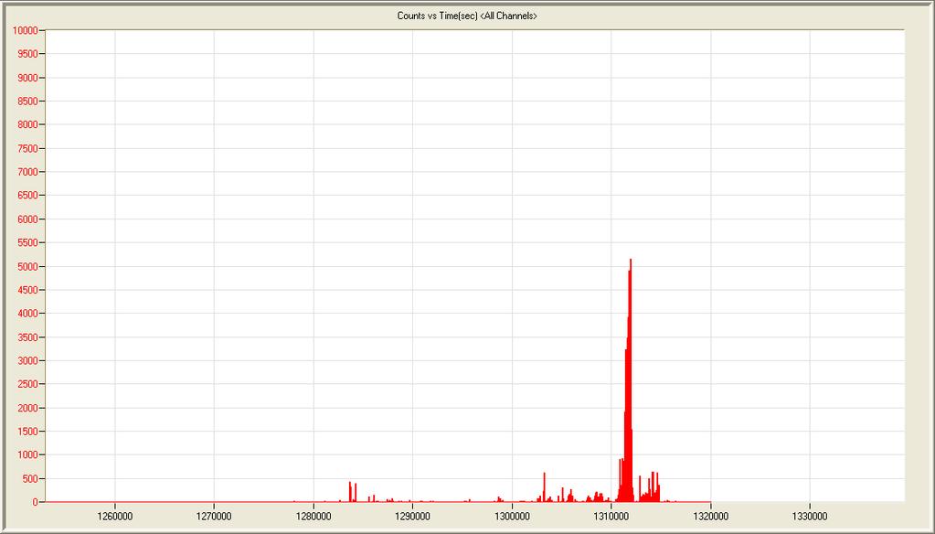
102 (a) (b) 89

103 (c) Figure 9.13: Count rate versus time for third data set in north system (a) Low activity day; (b) High activity day; (c) Anomalous day (a) (b) Figure 9.14: Count rate versus time for third data set in south system (a) Low activity day; (b) High activity day 90

104 The fourth relationship analyzed with the third fracture criterion set and using the third data set is duration versus amplitude as seen in Figures 9.9 and The fracture criterion associated with this plot is that a hit must exceed 90dB in amplitude and have duration of at least 30ms. This fracture criterion is similar to one in the first and second fracture criterion sets; however, the duration threshold was dropped from 50ms to 30ms in order for the criterion to be satisfied by the data for fracture beam tests BTN2 and BTS2. The fifth relationship analyzed with the third fracture criterion set is the correlation of the time for an event versus the location of the event. The events are filtered so that those with source amplitudes greater than 80dB are shown. The fracture criterion considered here is that two events must occur within 1.5 inches and 1.3 seconds of each other. Examples of this plot can be seen in Figures 9.15 and For these plots, the automated software scans for clusters where two events occur within the 1.5 inches and 1.3 seconds and indicates its findings by identifying the cluster. In these plots the vertical axis is the time (seconds) from the beginning of the data record, and the horizontal axis is the distance along the direction of the bridge girder (inches) from the southernmost sensor. (a) 91

105 (b) (c) Figure 9.15: Time versus event location for third data set using the third fracture criterion set in the north system showing source amplitudes greater than 80dB (a) Low activity day; (b) High activity day; (c) Anomalous day 92

106 (a) (b) Figure 9.16: Time versus event location for the third data set using the third fracture criterion set in the south system showing source amplitudes greater than 80dB (a) Low activity day; (b) High activity day The final relationship analyzed with the third fracture criterion set and using the third data set is time versus the position of the events. For this plot, all events are plotted regardless of their amplitude. The criterion associated with this plot is that 11 events must occur within 22 inches and 2.7 seconds of each other. For these plots, the automated software scans for clusters where 11 events occur within the 22 inches and 2.7 seconds 93

107 and indicates its findings by identifying the cluster. In these plots the vertical axis is the time (seconds) from the beginning of the data record, and the horizontal axis is the distance along the direction of the bridge girder (inches) from the southernmost sensor. (a) (b) 94

108 (c) Figure 9.17: Time versus event location for the third data set in the north system showing all events (a) Low activity day; (b) High activity day; (c) Anomalous day (a) 95

109 (b) Figure 9.18: Time versus event location for the third data set in the south system showing all events (a) Low activity day; (b) High activity day Tables 9.7 and 9.8 show the number of times each criterion was exceeded in each month. Criterion one and six are the most commonly exceeded because they rely solely on a high number of hits, and that condition is often created by AE noise. Criteria such as two and four are exceeded much less often, thus they play a more important role in identifying AE data from fracture. Tables 9.9 and 9.10 show the number days that a given number of criteria are exceeded. The number of criteria exceeded varies each day; however during no single day are all criteria exceeded, thus the criterion set lead to the conclusion that no fracture events were recorded in the third data set. 96

110 Table 9.7: Frequency of Exceedance for Individual Criteria using the Third Fracture Criterion Set and the Third Data Set in the North System Fracture Criteria Counts [number of days criterion is exceeded] Sample Size [days] Jun Jul Aug Total Table 9.8: Frequency of Exceedance for Individual Criteria using the Third Fracture Criterion Set and the Third Data Set in the South System Fracture Criteria Counts [number of days criterion is exceeded] Sample Size [days] Jun Jul Aug Total Table 9.9: Number of Days a Given Number of Criteria were Exceeded using the Third Fracture Criterion Set and the Third Data Set in the North System No. of Criteria Exceeded No. of Days % of Days

111 Table 9.10: Number of Days a Given Number of Criteria were Exceeded using the Third Fracture Criterion Set and the Third Data Set in the South System No. of Criteria Exceeded No. of Days % of Days

112 CHAPTER 10 EFFECTIVENESS OF FRACTURE CRITERIA 10.1 Definition of Effectiveness In the following chapter the effectiveness of each fracture criterion set will be demonstrated using a tabular format to easily compare the three sets. Two types of effectiveness measures are calculated in this chapter: (1) the effectiveness of the criterion set ( f ) to identify a fracture, and (2) the effectiveness of the criterion set ( r ) to reject non-fracture AE signals. The effectiveness to identify fracture, f, is determined by using the criterion sets in situations where fracture was known to occur, namely the fracture beam tests. The effectiveness to reject non-fracture AE data, r, is determined by using the criterion sets in situations where fracture is known not to have occurred, namely the AE data collected in the bridge when fracture tests were not being conducted. These metrics are appropriate for the evaluation of the fracture criterion sets because accurate fracture criteria must be able to effectively identify fracture when it occurs (fracture beam tests) and to reject non-fracture AE signals when fracture does not occur (i.e. bridge data). The effectiveness to identify fracture, f, is defined from AE data recorded during the fracture beam tests as x f j ( ) = N T,i N T,t 100% [4] where j is the minimum number of criteria from the fracture criterion set that are met in N T,i fracture beam tests, and N T,t is the total number of fracture beam tests. As proposed here, f (j) should be equal to 100% when j = J = the maximum number of criteria in a given set (5 for set 1, and 6 for sets 2 and 3), because the notion is that all fracture criteria in a given set are triggered during a fracture event. Thus, to compare fracture criterion sets, only f (J) is needed. However, it is useful to evaluate f (j) when j < J and compare it among sets of criteria in order to see the rate (with respect to minimum number of criteria) at which the fracture criterion sets approach 100% effectiveness. 99

113 The effectiveness to reject non-fracture AE data, r, is defined from data collected in the bridge as x r ( j) = N - N D,t D,i 100% N D,t [5] where j is the minimum number of criteria from the fracture criterion set that are met during N D,i days and N D,i is the total number of days in the data set. As proposed here, r (j) should be equal to 100% when j = J = the maximum number of criteria in a given set (5 for set 1, and 6 for sets 2 and 3), because the notion is that none of the fracture criteria in a given set are triggered by AE data from non-fracture events recorded on the bridge. Thus, to compare fracture criterion sets, only r (J) is needed. However, it is useful to evaluate r (j) when j < J and compare it among sets of criteria in order to see the rate (with respect to minimum number of criteria) at which the fracture criterion sets approach 100% effectiveness. The effectiveness metrics f and r are loosely correlated. Assume that the parameters N T,i and N D,i are interchangeable, that is, N T,i = N D,i. That would correspond to a case in which exactly one fracture event occurs every day in a bridge. From Equations [5] and [6] it can be shown that r = 100 f. Of course, this idealized case is highly unrealistic for the Cedar Avenue Bridge, thus the two effectiveness metrics must be determined by independent means, fracture beam tests for f and data collected in the bridge for r Effectiveness of Fracture Criterion Sets in Identifying Fracture Each of the fully successful fracture beam tests (LT1, LT2, LT3, BTN2, and BTS2) is used to define the effectiveness to identify fracture, f, for the three fracture criterion sets. The evaluation is achieved using Equation [4] and is summarized in Tables In the tables, the effectiveness to identify fracture is calculated for a minimum number of criteria being used. The effectiveness value is calculated as the percentage of the tests where at least the minimum number of criteria is exceeded. For example, the use of only one or two criteria can indicate fracture in all fracture tests. Using a small number of 100

114 criteria (one or two) will result in a large number of false positives when applied to bridge data as shown in section 11.3, which is why numerous criteria are required (5 for set 1, and or 6 for sets 2 and 3). As more criteria are used, the effectiveness, r, of the first and second criteria sets decrease. This means that some of the criteria in these sets are not triggered even though fracture did occur in the test. For example the first criterion set, using all five criteria, can only successfully indicate fracture in 3 of the 5 of the tests ( r = 60%). This is possible because the BTN2 and BTS2 tests do not exceed all of the criteria for the first two criterion sets. Only the third criterion set can identify fracture with all 6 criteria in all of the fracture beam tests as seen in Table Showing the effectiveness for each number of criteria in Tables helps to illustrate how each additional criterion may decrease the probability of identifying fracture. Figure 10.1 provides a more striking illustration of the rate at which the various fracture criterion sets lose accuracy when a larger number of fracture criteria are required to be exceeded (i.e. increasing j). Clearly, fracture criterion set three does not lose accuracy to identify fracture over the entire range of j, even when j = J. Table 10.1: First Criterion Set Effectiveness to Identify Fracture Min. No. of Criteria Exceeded No. of Tests Effectiveness (%)

115 Table 10.2: Second Criterion Set Effectiveness to Identify Fracture Min. No. of Criteria Exceeded No. of Tests Effectiveness (%) Table 10.3: Third Criterion Set Effectiveness to Identify Fracture Min. No. of Criteria Exceeded No. of Tests Effectiveness (%) Figure 10.1: Fracture Effectiveness During Fracture Beam Tests 102

116 10.3 Effectiveness of Fracture Criterion Sets in Rejecting Non-Fracture AE Data The data from the data sets described in Chapter 9 where used to determine the effectiveness of the three criterion sets to reject non-fracture AE data obtained form the Cedar Avenue Bridge. Each criterion set was evaluated with its corresponding data set as described in Chapter 9 (i.e. first data set with first criterion set etc.). The effectiveness to reject non-fracture AE data, r. is defined using Equation [5]. For example in Table 11.4 at least one criterion is exceeded 109 days of the total 193 days during the data set. This means that using only one criterion a false positive would be produced 56 percent (109/193) of the time (i.e. using one criterion is 44 percent effective). Tables show the effectiveness of using a given minimum number of criteria to analyze bridge AE data. Note that the use of all criteria in each set is 100% effective, but calculating the effectiveness of using less than all criteria can help indicate the evolution of accuracy for each data set as the minimum number of fracture criteria increases. Figure 10.2 provides a more striking illustration of the rate at which the various fracture criterion sets gain accuracy when a larger number of fracture criteria are required to be exceeded (i.e. increasing j). Clearly, fracture criterion set three gains accuracy at a faster rate with j, especially when the AE data recorded with the South system is considered. Table 10.4: Non-Fracture AE Signal Rejection Effectiveness for First Criterion Set in South System Min. No. of Criteria Exceeded No. of Days Effectiveness (%)

117 Table 10.5: Non-Fracture AE Signal Rejection Effectiveness for Second Criterion Set in North System Min. No. of Criteria Exceeded No. of Days Effectiveness (%) Table 10.6: Non-Fracture AE Signal Rejection Effectiveness for Second Criterion Set in South System Min. No. of Criteria Exceeded No. of Days Effectiveness (%) Table 10.7: Non-Fracture AE Signal Rejection Effectiveness for Third Criterion Set in North System Min. No. of Criteria Exceeded No. of Days Effectiveness (%)

118 Table 10.8: Non-Fracture AE Signal Rejection Effectiveness for Third Criterion Set in South System No. of Criteria Exceeded No. of Days Effectiveness (%) Figure 10.2: Non-Fracture AE Signal Rejection Effectiveness from Bridge Data Sets 10.4 Discussion Upon analyzing the effectiveness of a fracture criterion set to identify AE signals that contain fracture events, the fewer the criteria in a set, the more likely it will be to identify a fracture event. However, this is so only because fewer criteria mean a more lenient threshold has to be overcome and instances of fracture event identification are, in reality, cases of false positives. On the other hand, when analyzing the effectiveness of a fracture criterion set to reject non-fracture AE events, the opposite is true. That is, the more fracture criteria are being used, the less likely a false positive will be identified. Thus, an optimal fracture criterion set must have near perfect effectiveness for both identifying 105

119 fracture ( f ~ 100%) and rejecting non-fracture AE events ( r ~ 100%). Based on the study reported in this document, a large number of relevant fracture criteria are needed (at least 5) for the sparse sensor application investigated here. For the fracture criterion sets developed here, Tables show that the third fracture criterion set is the most effective in identifying fracture: It does not lose fracture identification effectiveness for as many as six simultaneous fracture criteria being exceeded. Fracture criterion sets one and two were not able to identify fracture in the bridge fracture tests using all of their criteria. The third criterion set, in contrast, was able to identify the fracture events in all the fracture tests even with the maximum number of fracture criteria being used (xf(j) = 100%). Similarly, Tables of Section show that all fracture criterion sets are 100% effective in rejecting non-fracture AE signals ( r (J) = 100%) when all criteria are used (j = J). However, the third criterion set appears to be the most effective when fewer than the maximum number of criteria is used (j < J). For example, if one criterion is taken from each set, the third criterion set will still be nearly perfect, that is r (J - 1) = 99% and 100%, respectively, for the North and South Systems. The second fracture criterion set will be a little slightly less effective with r (J - 1) = 95% and 97%, respectively, for the North and South Systems. The first fracture criterion set is the worst performer with r (J - 1) = 93%. The superior performance of the third fracture criterion set is evaluated in Tables and illustrated in Figures 10.1 and The enhanced performance of this fracture criterion set is driven by increased utilization of the parameters that are available for calculation using Mistras AEwin software, as well as the more in-depth analysis of the collected AE data by checking individual sensors instead of sensor groups. 106

120 CHAPTER 11 - SUMMARY, CONCLUSIONS, AND RECOMMENDATIONS 11.1 Summary The goal of the project discussed in this report was to determine if acoustic emission (AE) technology can be used for sparse monitoring of fracture-critical steel bridges. This project followed two earlier phases that included system design in Phase I (Schultz & Thompson, 2010) and implementation of one 16-sensor system and preliminary data collection and processing in Phase II (Schultz et al., 2014). For this third phase of the overall program, a second AE system, which was nominally identical to the first one, was added and the two systems were used to collect AE data from one of the tie girders spanning the Minnesota River in the Cedar Avenue Bridge. AE data was collected from November 1 st, 2013 until October 31 st, The data collected by the two AE systems was then evaluated to assess the efficiency of data processing protocols relying on fracture criterion sets developed in this project and defined in Chapter 8 (Tables 8.1, 8.3 and 8.5). To quantify the characteristics of AE fracture data, several tests were performed in the laboratory, and other ones tested in the bridge, to determine threshold values for a series of parameters that were used to define fracture criteria for AE signals. In these tests (Chapter 6), notched steel beams were fractured and the AE signals were collected with the AE monitoring equipment. The AE data collected during the fracture tests were used to develop data processing protocols and evaluation criteria in the form of criteria that rely on AE parameters computed by software provided by the equipment manufacturer (Mistras AEWin TM ). The protocols and criteria were designed to discriminate between (1) true AE signals associated with steel fracture and (2) non-fracture AE signals recorded on the Cedar Avenue Bridge and generated by non-ae sources. Each data file containing non-fracture AE data recorded on the bridge was evaluated by counting the number of fracture criteria were exceeded. No AE data file recorded on the bridge, at times other than those for the fracture beam tests, exceeded all of the criteria in any of the three 107

121 fracture criteria sets. This observation is in agreement with the Cedar Avenue Bridge s history of excellent performance as determined by periodic visual inspections Conclusions The monitoring of the Cedar Avenue Bridge using AE technology demonstrated that, although AE processing protocols may be complex, AE technology holds promise for identifying fracture in steel bridges, particularly those bridges that are fracture-critical. To properly use AE to detect fracture, tests must be performed to simulate a fracture occurring in the bridge structure. In complicated geometries, such as the Cedar Avenue Bridge, AE waveforms from fracture are likely to become distorted and scattered before ever being detected by a sensor. This latter observation is especially important for sparse AE monitoring. Because of this wave distortion, no single trademark characteristic exists for an AE wave propagating from a fracture. However, all AE waves associated with fracture of beam tests in the laboratory and the bridge featured multiple characteristics that can and should be exploited to discriminate between fracture AE waves from nonfracture AE waves. Thus, multiple indications of fracture must be considered in order to determine the occurrence of fracture within a reasonable degree of accuracy. Examples of non-fracture AE waves include (1) high numbers of transient waveforms traveling though the medium, (2) large amounts of excitation in piezoelectric vibrating crystals, and (3) waveforms propagating from a localized region. After conducting this project the following conclusions can be made: 1. Despite inherent challenges, sparse AE sensor systems (i.e. with sensors placed at maximum spacing) can detect the occurrence of fracture even in a noisy environment such as a bridge given proper fracture criteria and the protocols to enforce them. 2. A sensor spacing of 10ft along the tie girder, determined from pencil break tests, proved to be adequate as verified by notched beam fracture tests conducted in the Cedar Avenue Bridge. 108

122 3. The fracture tests performed in the bridge produced AE data that does not match the AE data produced by the bridge under the range of conditions experienced during the monitoring periods. This feature was used to advantage by defining characteristics of the AE data from the fracture beam tests that was not present in the bridge data when fracture beams were not being tested at the bridge. 4. The final pair of bridge notched beam fracture tests provided strong evidence that a small amount of fracture can be detected by sensors spaced at 10ft along the bridge girder. 5. Continuous monitoring has a low probability of being achieved when the sole power source is an array of solar panels. Using the sensors to monitor a large area of the bridge structure proved to be a challenging task. Without the ability to filter AE noise from outside the monitoring region, the AE sensors where at the mercy of complex combinations of sound waves from a multitude of sources. Non-fracture sources were observed to produce very high hit rates at times and strong intensities at others. The key to discarding false positives from non-fracture sources is having multiple fracture criteria that target various characteristics of AE signals from fracture events, including location of the source of the AE activity. Despite the anomalous and high activity data sets discussed in Chapter 9, the AE system with far-spaced AE sensors and the proposed fracture criteria, particularly fracture criterion set three, holds promise for differentiating fracture and non-fracture AE events in steel bridges. It may be necessary to perform some fracture tests, using the notched beam test developed as part of this study, when implementing far-spaced AE sensor systems in other bridges Recommendations The following recommendations are offered in regards to future use or research concerning the use AE sensor systems in fracture-critical steel bridges, especially if a sparse sensor network is being considered. 109

123 The fracture tests used in this project to determine AE fracture characteristics have used a test specimen that is acoustically connected to the bridge. This test setup is an efficient means to simulate a fracture in the bridge when fracture is sudden and stress concentration factors are high. These tests, however, may produce AE data with different characteristics if the beam is loaded in cycles to fatigue failure. Further experimentation should be conducted on fatigue fracture in both a laboratory setting and on an in-service bridge to help determine if the protocols and criteria developed in this project are applicable to fracture from fatigue, or if different fracture criteria and data processing protocols are needed for fatigue crack detection. Experiments have been conducted by others to monitor the local behavior of flexural members that develop fatigue cracking, but an experiment implementing sparse AE sensor systems have not been used yet for monitoring fatigue cracking. Solar power is not recommended under most, if not all, circumstances to be the sole source of power for an AE monitoring system. Problems will occur if large arrays of solar panels are installed adjacent to heavily traveled roads because, as was experienced in this project, ice, snow, de-icing salts and other road debris, as well as vandalism, are believed to have caused damage on multiple occasions to the solar panels. Moreover, protective wire meshes, installed to avoid most of the observed damage to the solar panels, reduced the amount of incident sunlight on the panels. Even when the solar panels were not damaged, they were unable to continuously power the AE systems in this experiment because of the lack of sun and snow/ice cover in the winter, reduced incident sunlight from the wire meshes, and shadowing from the bridge members and nearby trees. For these reasons, a power supply that can support continuous monitoring is essential to assure that the monitoring system is operational if fracture occurs. It is recommended that the system be powered with a standard 120V, 60Hz alternating current from a reliable source such as the local electrical utility network. A land-based internet connection is recommended to insure that the monitoring system is always accessible for a remote login and/or data upload. Wireless connection are less reliable that land-based internet connections and often suffer communication 110

124 interruptions. Furthermore, wireless modem antennas are susceptible to factors such as vandalism, damage during bridge maintenance and equipment failure. If continuous monitoring is desired, the SH-II will need to upload files for replay to a website at specified time intervals. In order to detect fracture, bridge AE data should be analyzed daily. The AEwin software has commands and options that can be used to facilitate this activity: the auto file-close criteria of AEwin should be set to close and reopen after an elapsed time of 24 hours, and the use continued files box should be unchecked to avoid redefining time domain boundaries for every analysis. The AEwin software proved to be a powerful tool for analyzing data that had already been collected. However, the graphical interface of the software is designed with a bias toward analyzing data from a test rather than monitoring a structure over a long period of time. Suggestions are provided below to facilitate the use of the graphical interface in the AEWin TM software. First, normalization of the duration of time steps is recommended in order to have results comparable from one data file to another. Second, for continuous monitoring, the software must be set to create a new data file with a new timer for each day. 111

125 REFERENCES MISTRAS Products and Systems Division. (2010). R15l-AST Sensor Integral Preamplifier Acoustic Emission Sensor. Princeton Junction, NJ: MISTRAS. Barsoum, F. F., Suleman, J., Karcak, A., & Hill, E. V. (2009). Acoustic Emission Monitoirng and Fatigue Life Prediction in Axially Loaded Notched Steel Specimens. Acoustic Emission Group, Beattie, A. G. (2013). Acoustic Emission Non-Destructive Testing of Structures using Source Location Techniques. Albuquerque, NM and Livermore, CA: Sandia National Laboratories. Bohse, J. (2013). Acoustic Emission. In H. Czichos, Handbook of Technical Diagnostics (pp ). Springer Berlin Heidelberg. Colombo, I. S., Main, I. G., & Forde, M. C. (2003). Assessing Damage of Reinforced Concrete Beam Using "b-value" Analysis of Acoustic Emission Signals. Journal of Materials in Civil Engineering, Hellier, C. J. (2012). Chapter 10: Acoustic Emission Testing. In C. J. Hellier, & M. Shakinovsky, Handbook of Nondestructive Evaluation (pp ). The McGraw-Hill Companies. Higgins, C. M., Senturk, E. A., & Turan, T. O. (2010). Comparison of Block-Shear and Whitmore Section Methods for Load Rating Existing Steel Truss Gusset Plate Connections. Journal of Bridge Engineering, Hopwood II, T., & Prine, D. W. (1987). Acoustic Emission Monitoring of In-Service Bridges. Frankfort, KY: Kentucky Transportation Cabinet. Hopwood, II, T., & Prine, D. W. (1987). Acoustic Emission Monitoring of In-Service Bridges. Frankfort, KY: Kentucky Transportation Cabinet. Kaiser, J. (1950). Untersuchung über das Auftreten von Geräuschen beim Zugversuch. München : Fakultät für Maschinenwesen und Elektrotechnik der Technischen Universität München. Kosnik, D. E. (2009). Acoustic Emission Testing of a Difficult-to-Reach Steel Bridge Detail. Journal of Acoustic Emisison, Maji, A. K., Satpathi, D., & Kratochvil, T. (1997). Acoustic Emission Source Location Using Lamb Wave Modes. Journal of Engineering Mechanics,

126 McKeefry, J., & Shield, C. (1999). Acoustic Emission Monitoring of Fatigue Cracks in Steel Bridge Girders. St. Paul: Minnesota Department of Transportation. Miller, R. K., & McIntire, P. (1987). Nondestructive Testing Handbook, Volume 5: Acoustic Emission Testing. American Society for Nondestructive Testing. Nair, A., & Cai, C. S. (2010). Acoustic Emission Monitoring of Bridges: Review and Case Studies. Engineering Structures, Physical Acoustics Corporation. (2010). Solar Powered Sensor Highway System User's Manual Rev 1. Princeton Junction, NJ: Physical Acoustics Corporation. Pollock, A. A. (2003). Acoustic Emission Inspection. Princeton Jct, NJ: MISTRAS Holdings Group. Schultz, A. E., Morton, D. L., Tillmann, A. S., Campos, J. E., Thompson, D. J., Lee- Norris, A. J., & Ballard, R. M. (2014). Acoustic Emission Monitoring of a Fracture-Critical Bridge. St. Paul: Minnesota Department of Transportation. Schultz, A., & Thompson, D. (2010). Development of an Advanced Structural Monitoring System. St. Paul, MN: Minnesota Department of Transportation. Scruby, C. B. (1987). An Introduction to Acoustic Emission. Instrument Science and Technology, Sinclair, A. C., Connors, D. C., & Formby, C. L. (1977). Acoustic Emission Analysis during Fatigue Crack Growth in Steel. Materials Science and Engineering, 28, Yilmaz, A. (2011). The Portevin Le Chatelier effect:. Science and Technology of Advanced Materials, Yu, Z., Ziehl, P., Zarate, B., & Caicedo, J. (2011). Prediction of fatigue crack growth in steel bridge components using acoustic emission. Journal of Constructional Steel Research,

127 APPENDIX A: FRACTURE BEAM TEST RESULTS 114

128 This appendix documents the results of all of the notched beam fracture tests performed for this project. LT1, LT2, and LT3 are the names of the tests performed in the Theodore V. Galambos Structures Laboratory in the Department of Civil, Environmental and Geo- Engineering at the University of Minnesota. BTN1, BTN2, BTS1, and BTS2 are the names of the fracture beam tests performed within the Cedar Avenue Bridge. For each parameter only certain sensor results are applicable in determining characteristics of bridge fracture data. Tables A-1 through A-4 along with Figure A.1 must be referred to in order to understand the relevance of each sensor in each of the plots. Only the sensors that realistically simulate bridge fracture are used in creating the fracture criteria, but this section includes additional sensor data for completeness. Value eligible for determining criteria Value not eligible for determining criteria Value irrelevent due to fracture notched beam debonding Figure A.1: Fracture Test Results Key Table A.1: Laboratory Fracture Test Results Hit Rate [hits/s] Energy Rate [pj/s] Count Rate [counts/s] Sensor LT1 LT2 LT3 LT1 LT2 LT3 LT1 LT2 LT

129 Table A.2: North System Bridge Fracture Test Results Hit Rate [hits/s] Energy Rate [pj/s] Count Rate [counts/s] Sensor BTN1 BTN2 BTN1 BTN2 BTN1 BTN Table A.3: South System Bridge Fracture Test Results Hit Rate [hits/s] Energy Rate [pj/s] Count Rate [counts/s] Sensor BTS1 BTS2 BTS1 BTS2 BTS1 BTS Table A.4: Number of hits with duration > 30ms and amplitude > 90dB for each test Test LT1 LT2 LT3 BTN1 BTN2 BTS1 BTS2 Sensor(s) 8 7,8 7, Hits>30ms &>90dB

130 A.1 Laboratory Test Number 1 (LT1) Figure A.2: Cumulative Hits versus Time [s] (sensors 6,7,8) Figure A.3: Cumulative Hits versus Time [s] (individual sensors) 117

131 Figure A.4: Cumulative Hits versus Frequency Centroid [khz] (all sensors) Figure A.5: Duration [μs] versus Amplitude [db] (sensor 8) 118

132 Figure A.6: Maximum Absolute Energy [aj] versus Amplitude [db] (sensor 8) Figure A.7: Absolute Energy Rate [aj/s] during 86 second period including fracture (sensor 6,7,8) 119

133 Figure A.8: Absolute Energy Rate [aj/s] during 86 second period including fracture (individual sensors) Figure A.9: Count Rate [counts/s] during 86 second period including fracture (individual sensors) 120

134 Figure A.10: Time [s] versus x-position [in] on notched beam x = 0 at crack tip Figure A.11: Time [s] versus x-position [in] on notched beam; x = 0 at crack tip; events with source amplitude greater than 80dB only 121

135 A.2 Laboratory Test Number 2 (LT2) Figure A.12:Cumulative Hits versus Time [s] (sensors 4,5,6,7,8) Figure A.13:Cumulative Hits versus Time [sec] (individual sensors) 122

136 Figure A.14:Hits versus Frequency Centroid [khz] (all sensors, during fracture) Figure A.15:Duration [μs] versus Amplitdue [db] (sensors 7,8) 123

137 Figure A.16: Maximum Absolute Energy [aj] versus Amplitude [db] (sensors 7,8) Figure A.17: Absolute Energy Rate [aj/s] during 86 second period including fracture (sensors 7,8) 124

138 Figure A.18: Absolute Energy Rate [aj/s] during 86 second period including fracture (individual sensors) Figure A.19: Count Rate [counts/s] during 86 second period including fracture (individual sensors) 125

139 Figure A.20: Time [s] versus x-position [in] on girder; x = 0 at fracture beam Figure A.21: Time [s] versus x-position [in] on girder; x = 0 at fracture beam; events with source amplitude greater than 80dB only 126

140 A.3 Laboratory Test Number 3 (LT3) Figure A.22: Cumulative Hits versus Time [s] (sensors 4,5,6,7,8) Figure A.23: Cumulative Hits versus Time [s] (individual sensors) 127

141 Figure A.24: Hits versus Frequency Centroid [khz] (all sensors, during fracture) Figure A.25: Duration [μs] versus Amplitude [db] (sensors 7,8) 128

142 Figure A.26: Maximum Absolute Energy [aj] versus Amplitude [db] (sensors 7,8) Figure A.27: Absolute Energy Rate [aj/s] during 86 second period including fracture (sensors 7,8) 129

143 Figure A.28: Absolute Energy Rate [aj/s] during 86 second period including fracture (individual sensors) Figure A.29: Count Rate [counts/s] during 86 second period including fracture (individual sensors) 130

144 Figure A.30: Time [s] versus x-position [in] on notched beam; x = 0 at crack tip; events with source amplitude greater than 80dB only Figure A.31: Time [s] versus x-position [in] on notched beam; x = 0 at crack tip 131

145 A.4 Bridge Test North System Number 1 (BTN1) Figure A.32: Cumulative Hits versus Time [s] (sensors 8,9,10,11) Figure A.33: Cumulative Hits versus Time [s] (individual sensors) 132

146 Figure A.34: Hits versus Frequency Centroid [khz] (all sensors, during fracture) Figure A.35: Duration [μs] versus Amplitude [db] (sensors 8,9,10,11) 133

147 Figure A.36: Maximum Absolute Energy [aj] versus Amplitude [db] (sensors 8,9,10,11) Figure A.37: Absolute Energy Rate [aj/s] during 86 second period including fracture (sensors 8,9,10,11) 134

148 Figure A.38: Absolute Energy Rate [aj/s] during 86 second period including fracture (individual sensors) Figure A.39: Count Rate [counts/s] during 86 second period including fracture (individual sensors) 135

149 A.5 Bridge Test South System Number 1 (BTS1) Figure A.40: Cumulative Hits versus Time [s] (sensors 6,7,8,9) Figure A.41: Cumulative Hits versus Time [s] (individual sensors) 136

150 Figure A.42: Hits versus Frequency Centroid [khz] (all sensors, during fracture) Figure A.43: Duration [μs] versus Amplitude [db] (sensors 6,7,8,9) 137

151 Figure A.44: Maximum Absolute Energy [aj] versus Amplitude [db] (sensors 6,7,8,9) Figure A.45: Absolute Energy Rate [aj/s] during 86 second period including fracture (sensors 6,7,8,9) 138

152 Figure A.46: Absolute Energy Rate [aj/s] during 86 second period including fracture (individual sensors) Figure A.47: Count Rate [counts/s] during 86 second period including fracture (individual sensors) 139

153 A.6 Bridge Test North System Number 2 (BTN2) Figure A.48: Cumulative Hits versus Time [s] (sensors 8,9,10,11) Figure A.49: Cumulative Hits versus Time [s] (individual sensors) 140

154 Figure A.50: Hits versus Frequency Centroid [khz] (all sensors, during fracture) Figure A.51: Duration [μs] versus Amplitude [db] (sensors 8,9,10,11) 141

155 Figure A.52: Maximum Absolute Energy [aj] versus Amplitude [db] (sensors 8,9,10,11) Figure A.53: Absolute Energy Rate [aj/s] during 86 second period including fracture (sensors 8,9,10,11) 142

156 Figure A.54: Absolute Energy Rate [aj/s] during 86 second period including fracture (individual sensors) Figure A.55: Count Rate [counts/s] during 86 second period including fracture (individual sensors) 143

157 Figure A.56: Time [s] versus Event Position [in] (only events with source amplitude > 80dB shown) Figure A.57: Time [s] versus Event Position [in] (all events) 144

158 A.7 Bridge Test South System Number 2 (BTS2) Figure A.58: Cumulative Hits versus Time [s] (sensors 6,7,8,9) Figure A.59: Cumulative Hits versus Time [s] (individual sensors) 145

159 Figure A.60: Hits versus Frequency Centroid [khz] (all sensors, during fracture) Figure A.61: Duration [μs] versus Amplitude [db] (sensors 6,7,8,9) 146

160 Figure A.62: Maximum Absolute Energy [aj] versus Amplitude [db] (sensors 6,7,8,9) Figure A.63: Absolute Energy Rate [aj/s] during 86 second period including fracture (sensors 6,7,8,9) 147

161 Figure A.64: Absolute Energy Rate [aj/s] during 86 second period including fracture (individual sensors) Figure A.65: Count Rate [counts/s] during 86 second period including fracture (individual sensors) 148

162 Figure A.66: Time [s] versus Event Position [in] (only events with source amplitude > 80dB shown) Figure A.67: Time [s] versus Event Position [in] (all events) 149