Solar Photovoltaic System Modeling and Control

Transcription

1 University of Denver Digital DU Electronic Theses and Dissertations Graduate Studies Solar Photovoltaic System Modeling and Control Qing Xia University of Denver Follow this and additional works at: Recommended Citation Xia, Qing, "Solar Photovoltaic System Modeling and Control" (2012). Electronic Theses and Dissertations This Thesis is brought to you for free and open access by the Graduate Studies at Digital DU. It has been accepted for inclusion in Electronic Theses and Dissertations by an authorized administrator of Digital DU. For more information, please contact jennifer.cox@du.edu.

2 SOLAR PHOTOVOLTAIC SYSTEM MODELING AND CONTROL A Thesis Presented to The Faculty of Engineering and Computer Science University of Denver In Partial Fulfillment of the Requirements for the Degree Master of Science by Qing Xia November 2012 Advisor: David Wenzhong Gao

3 Author: Qing Xia Title: SOLAR PHOTOVOLTAIC SYSTEM MODELING AND CONTROL Advisor: David Wenzhong Gao Degree Date: November 2012 ABSTRACT To realize the benefits of grid-connected photovoltaic system, it is extremely important to reduce energy losses and improve reliability of grid-connected PV systems with high PV penetration. In this thesis, three different Maximum Power Point Tracking (MPPT) strategies named as Perturbation & Observation MPPT, Incremental Conductance MPPT and Fuzzy Logic Control MPPT have been analyzed, simulated and compared with each other to improve the efficiency of power conversion. A general discussion to counteract partial shading effect in several aspects is also provided in this thesis. In order to improve reliability of the system, an optimum current control loop with suitable control parameters are achieved by comparing three different PI controller parameter design methods, including self-tuning method, trial and error method and mathematical analysis method. Considering the complexity brought by modulation and demodulation process between abc stationary frame and dq0 synchronous frame of PI control loop, P+ Resonant controller, with simple control loop structure and zero steadystate error is also designed in this thesis. At last, LCL filter is analyzed and modeled under both steady state and disturbing condition. The effects of LCL filter for improving disturbance rejection capability and dynamic performance of the system is verified. ii

4 TABLE OF CONTENTS ABSTRACT... ii LIST OF FIGURES...v LIST OF TABLES... ix ACKNOWLEDGEMENTS...x CHAPTER 1: INTRODUCTION Introduction Organization of Thesis:...4 CHAPTER 2: PV ARRAY ANALYSIS AND MODELING PV Array Output Characteristics PV Array Modeling in PSCAD/EMTDC PV Array Output Results CHAPTER 3: MPPT ANALYSIS & MODELING Introduction of Maximum Power Point Tracking Perturbation and Observation MPPT strategy Fuzzy Logic Control MPPT Strategy Conclusion CHAPTER 4: SHADING EFFECTS AND APPLICATION OF POWER ELECTRONICS Introduction of Shading Effects [4-1] Study and Analysis to reduce Shading Effects Modeling of Partially Shaded PV array Introduction of DC-DC Converter [4-4] CHAPTER 5: CONTROL LOOP DESIGN FOR GRID CONNECTED VOLTAGE SOURCE INVERTER WITH LCL FILTER Basic Analysis of Grid-Connected VSI (Voltage Source Inverter) Control Strategy Design for Three-Phase Grid Connected VSI Analysis and Design of PI Controller s parameters Introduction of P+ Resonant Controller Control Strategy Design for Three Phase P+ Resonant Controller Analysis of the LCL Filter CHAPTER 6: CONCLUSTION AND FUTURE WORK Conclusion iii

5 6.2 Future work REFERENCES APPENDIX Appendix 2.1 PV Array System Modeling in PSCAD Appendix 3.1 P&O MPPT Strategy Model in Constant Condition Appendix 3.1 P&O MPPT Strategy Model in Constant Condition (.m) Appendix 3.2 P&O MPPT Strategy Model in Temperature Varying Condition Appendix 3.2 P&O MPPT Strategy Model in Temperature Varying Condition (.m) Appendix 3.2 P&O MPPT Strategy Model in Irradiation Varying Condition Appendix 3.2 P&O MPPT Strategy Model in Irradiation Varying Condition (m.). 136 Appendix 3.3 FIS Design of Fuzzy Logic Control MPPT Strategy Appendix 3.4 Comparison Model of P&O MPPT Strategy, IncCond MPPT Strategy and FLC MPPT Strategy Appendix 3.5 Responding Results of Comparison between P&O MPPT Strategy, IncCond MPPT Strategy and FLC MPPT Strategy in Constant Condition (.m) Appendix 3.6 Re-regulation of FIS Appendix 3.7 The Output Curve of Comparison between P&O MPPT Strategy, IncCond MPPT Strategy and FLC MPPT Strategy in Both Temperature and Irradiation Varying Condition Appendix 4.1 Shading Main Program: PVprog [4-2] Appendix 4.2 Processing Time Varying Data from MATLAB M.file to SIMULINK Appendix 5.1Tuning Results of PID Controller Appendix 5.2 System synchronous frame control with PI controller in PSCAD Appendix 5.3 Analysis of Each Control Parameter Appendix 5.4 Relationship Between Damping Ratio ζ and Natural Frequency ω Appendix 5.5 Calculation of Controller Parameters Appendix 5.6 PI Parameter Design and System Analysis Process Appendix 5.7 P+ Resonant Controller Parameter Test and System Analysis Process Appendix 5.8 Bode Plot Diagram of Both PI Controller and P+ Resonant Controller at Fundamental Frequency Appendix 5.9 Comparison Between PI Controller and P+ Resonant Controller under Disturbing Condition Appendix 5.10 LCL Filter Parameter Analysis iv

6 LIST OF FIGURES Fig. 2.1 A simple equivalent circuit for a photovoltaic cell...7 Fig. 2.2 I-V curve of a single PV cell Fig. 2.3 P-V curve of a single PV cell Fig. 2.4 Output I-V curve of PV array at S=1000, T1=233.0, T2=293.0, T3=353.0 (Modeled in PSCAD) Fig. 2.5 Output P-V curve of PV array at S=1000, T1=233.0, T2=293.0, T3=353.0 (Modeled in PSCAD Fig. 2.6 Output I-V curve of PV array at T=293; S1=300, S2=600, S3=1000 (Modeled in PSCAD) Fig. 2.7 Output P-V curve of PV array at T=293; S1=300, S2=600, S3=1000 (Modeled in PSCAD) Fig.3.1 the principle of P&O MPPT strategy Figure.3.2 flowchart of P&O MPPT strategy Fig.3.3 control model of P&O MPPT strategy Fig.3.4(a) output I-V curve of P&O MPPT strategy in constant condition T=290K, G= Fig. 3.4(b) output P-V curve of P&O MPPT strategy in constant condition T=290K, G= Fig.3.5(a) output I-V curve of P&O MPPT strategy in varying temperature condition Fig.3.5(b) output P-V curve of P&O MPPT strategy in temperature varying condition.. 19 Fig.3.5(c) zoomed in figure of output P-V curve of P&O MPPT strategy in temperature varying condition (first group) Fig.3.6(a) output I-V curve of P&O MPPT strategy in varying irradiation condition Fig.3.6(b) output P-V curve of P&O MPPT strategy in irradiation varying condition Figure. 3.7(a) Output I-V curve for analysis of MPPT when. Fig. 3.7(b) Output P-V curve for analysis of MPPT when Fig.3.8 flow chart of IncCond MPPT strategy Fig.3.9 control model of IncCond MPPT strategy Fig.3.10(a) output I-V curve of IncCond MPPT strategy under constant condition T=290K, G= Fig.3.10(b) output P-V curve of IncCond MPPT strategy under constant condition T=290K, G= Fig.3.11(a) output I-V curve of IncCond MPPT strategy under constant condition with large reference value Fig.3.11(b) output P-V curve of IncCond MPPT strategy under constant condition with large reference value Fig.3.12(a) output I-V curve of IncCond MPPT strategy under varying temperature condition Fig.3.12(b) output P-V curve of IncCond MPPT strategy under varying temperature condition v

7 Fig.3.13(a) output I-V curve of IncCond MPPT strategy under varying irradiation condition Fig.3.13(b) output P-V curve of IncCond MPPT strategy under varying irradiation condition Fig.3.14 principle of fuzzy logic control (FLC) MPPT strategy Fig FIS surface of fuzzy logic control MPPT strategy Fig control model of FLC MPPT strategy Fig. 3.17(a) output I-V curve of FLC MPPT strategy under constant condition T=290K, G= Fig. 3.17(b) output P-V curve of FLC MPPT strategy under constant condition T=290K, G= Fig.3.18(a) output I-V curve of FLC MPPT strategy under varying temperature condition Fig.3.18(b) output P-V curve of FLC MPPT strategy under varying temperature condition Fig.3.19(a) output I-V curve of FLC MPPT strategy under varying irradiation condition Fig.3.19(b) output P-V curve of FLC MPPT strategy under varying irradiation condition Fig. 3.20(a) output I-V curve of FLC MPPT strategy under small range varying irradiation condition Fig. 3.20(b) output V-P curve of FLC MPPT strategy in small range varying irradiation condition Fig actual power variation in decreasing irradiation condition v.s. designed grades of power variation Fig. 3.22(a) output I-V curve of comparison between P&O MPPT strategy, IncCond MPPT strategy and FLC MPPT strategy in constant condition Fig. 3.22(b) output P-V curve of comparison between P&O MPPT strategy, IncCond MPPT strategy and FLC MPPT strategy in constant condition Fig.3.23 responding results of comparison between P&O MPPT strategy, IncCond MPPT strategy and FLC MPPT strategy in constant condition Fig new responding results of comparison between P&O MPPT strategy, IncCond MPPT strategy and FLC MPPT strategy in constant condition Fig. 3.25(a) = Fig. 3.25(b) = Fig. 3.26(a) output curve of comparison between P&O MPPT strategy, IncCond MPPT strategy and FLC MPPT strategy under varying temperature condition Fig. 3.26(b) output curve of comparison between P&O MPPT strategy, IncCond MPPT strategy and FLC MPPT strategy under varying irradiation condition Fig.4.1 comparison of voltage current characteristics of PV string operating in uniform condition and non-uniform condition [4-1] Fig.4.2 bypass diode across the PV cells when one cell is shaded vi

8 Fig.4.3 PV array configuration for alleviating the power loss under partial shading condition (a) SP, (b) TCT, (c) BL Fig.4.4 Decomposition of Reconfigurable PV array Fig. 4.5 PV system architecture (a) Centralized, (b) Series-Connected Micro-converter, (c) Parallel-Connected Micro-converter, (d) Micro-inverter Fig. 4.6 unique global power maximum strategy Fig. 4.7 Load-Line Maximum Power Point Tracking Algorithm Fig. 4.8 Power Increment Technique Fig. 4.9 Partially Shaded PV array Configuration for test Fig. 4.10(a) I-V characteristics for subassemblies of Group Fig. 4.10(b) P-V characteristics of subassemblies of Group Fig. 4.11(a) I-V characteristics for subassemblies of Group Fig. 4.11(b) P-V characteristics for subassemblies of Group Fig. 4.12(a) I-V characteristics for subassemblies of Group Fig. 4.12(b) P-V characteristics for subassemblies of Group Fig. 4.13(a) I-V characteristics of series assemblies Fig. 4.13(b) P-V characteristics of series assemblies Fig. 4.14(a) I-V characteristics of group Fig. 4.14(b) P-V characteristics of group Fig. 4.15(a) I-V characteristics of PV array Fig. 4.15(b) P-V characteristics of PV array Fig Boost converter schematic [4-5] Fig Regulation result of the DC-DC converter in PSCAD Fig. 5.1 Overall VSI structure in relation to LCL filter Fig. 5.2 Equivalent circuit of grid connected VSI with LCL filter in the system Fig. 5.3 abc to dq0 transformation [5-2] Fig.5.4 control strategy of a three-phase synchronous frame PI controlled VSI Fig. 5.5 Self-tuning method of three-phase grid connected VSI PI controller parameter design Fig. 5.6 Detected Maximum Power Point Voltage under Constant Environmental Condition Fig. 5.7 DC side Voltage under constant environmental condition Fig.5.8 Grid-connected Three-phase Current and Voltage Curves under constant environmental condition Fig. 5.9 Grid-connected Real Power under constant environmental condition Fig Grid-connected Reactive under constant environmental condition Fig MPPT Process under Randomly Changing Illumination Level Fig MPPT Results under Randomly Changing Illumination Level Fig DC Side Voltage when Illumination Level is changing Fig Gird-connected Three-phase Current and Voltage Curves when Illumination Level is changing Fig Grid-connected Real Power When Illumination Level in Changing Fig Grid-connected Reactive Power when Illumination Level is changing vii

9 Fig Single-phase control loop of grid connected VSI with LCL filter [5-4] Fig Zero-pole figure of control loop with variation of in overall view Fig Zero-pole figure of control loop with variation of in zoomed in view Fig step response of control loop with variation of Fig Zero-pole figure of control loop with variation of Fig step response figure of control loop with variation of Fig Zero-pole figure of control loop with variation of Fig step response figure of control loop with variation of Fig Relationship between damping ratio ζ and natural frequency ω Fig Zero-pole figure of control loop with designed parameters Fig step response figure of control loop with designed parameters Fig Root locus figure of control loop with designed parameters Fig Bode Diagram of the system with designed parameters Fig demodulating single-phase integral block [5-11] Fig Two current feedback control strategy for single phase system Fig zero-pole figure of control loop with P+ Resonant Controller Fig root locus figure of control loop with P+ Resonant Controller Fig Step response figure of control loop with P+ Resonant controller Fig Bode Diagram of control loop with P+ Resonant controller Fig Bode diagram of PI and P+ Resonant Controller Fig Performance of PI controller v.s. P+ Resonant Controller under fundamental frequency Fig P+ Resonant controller performance of dynamic tracking Fig FFT analysis of grid current Fig zero-pole loop of varying L Fig Step response of varying L Fig Bode plot of varying L Fig zero-pole figure of varying L Fig Step response figure of varying L Fig Bode plot of varying L Fig Zero-pole figure of varying Cf Fig Step response figure of varying Cf Fig Bode plot figure of varying Cf Fig.5.49 Bode plot of Harmonic Impedance Fig FFT analysis of initial LCL filter reflection to the disturbance of 122 Fig FFT analysis of compared LCL filter reflection to the disturbance of viii

10 LIST OF TABLES Table 2.1 Data of PV module parameters [2-2]...8 Table 2.2 Data of PV array structure...9 Table 3.1 test parameters of varying temperature condition Table 3.2 test parameters of varying irradiation condition Table 3.3 Fuzzy logic control rule table Table 4.1 Partially Shaded PV array data analysis Table 5.1 Control Parameters of Trial and error method in PSCAD Table 5.2 Location of zeros and poles with variation of Table 5.3 Location of zeros and poles with variation of Table 5.4 Location of zeros and poles with variation of Table 5.5 Data summary of Varying L Table 5.6 Data summary of Varying L Table 5.7 data table summary of Varying Cf Table 5.8 Data summary of Harmonic Impedance ix

11 ACKNOWLEDGEMENTS I am grateful to my advisor, Dr. David Wenzhong Gao for his priceless insight into research and providing invaluable guidance, support and advice without which this thesis research project would have been almost impossible to complete. I must thank my colleagues for their support and help with my modeling. My gratitude is also extended to the staff of ECE department for their assistance. Finally, I am grateful to my parents for their support and inspiration. x

12 CHAPTER 1: INTRODUCTION 1.1 Introduction Today, PV systems are widely applied to off-grid generation applications [1-1] such as traffic warning lights, telecommunications, security systems and so on. Normally, when the electricity demand exceeds the supply of PV system, wind system or conventional electric generator can be added with PV system to create a hybrid system. In this case, PV system could be developed to provide power for remote area without or with poor supply from power grid. PV system has many benefits including portability, low operating costs, environmental benefits, stand-alone capability, modularity, safety and reliability, etc. While the basic expected application of PV system in worldwide is to achieve the stand-alone PV system, some highly industrialized countries such as the US, the European countries and Japan have already realized the grid-connected photovoltaic systems [1-2]. However, comparing with other renewable energy resources, photovoltaic generated electricity is still more expensive. In this case, it is extremely important to reduce energy losses and improve reliability of PV systems. This thesis studies and 1

13 analyzes the grid-connected PV system and attempts to find more reasonable solutions to solve those problems. Starting from PV array analysis and modeling, chapter 2 simulates the relationship between PV array s output characteristics and environmental conditions, which is considered as a fundamental knowledge for the subsequent MPPT algorithm study and partial shading effect study. When photovoltaic panels work under different temperature and illumination level, each photovoltaic panel will generate unique characteristic curve since the output power of photovoltaic panel varies as a function of the output voltage. Each photovoltaic panel has a unique maximum power point. At the maximum power point, the corresponding voltage changes as environmental temperature or irradiation level changes. Thus, it is necessary to track the maximum power point of the PV array in order to maintain a high output power efficiency of the PV generation system. Considering the high installation cost of PV array, the process of tracking Maximum Power Point maximizes the efficiency of photovoltaic energy system in photovoltaic conversion process. All in all, the MPPT process helps reduce the system cost and in the meantime enhance conversion efficiency. Three different MPPT algorithms have been carefully studied and analyzed in chapter 3 which includes the Perturbation and Observation (P&O) MPPT strategy, Incremental Conductance (IncCond) MPPT strategy and Fuzzy Logic Control (FLC) MPPT strategy [3-5] [3-6]. these MPPT strategies are analyzed and compared with each other in MATLAB SIMULINK under different environmental conditions, such as 2

14 varying temperature, varying irradiation level and varying both temperature and irradiation level. In the same chapter, a comparison on reliability as well as algorithm speed has been carried out between those three methods. Shading effects is another serious problem for the photovoltaic array distributed generation system, especially for large scale installation of PV array. Generally speaking, the total efficiency of photovoltaic generation conversion will be reduced due to partial shading. This kind of energy waste could bring very serious economic problems considering the high cost of PV investment. When parts of the PV array are shaded which is defined as partial shading, it could lead to hot spot problem which poses a severe damage to the PV array. If excessive heating problem exists for a certain period of time, the PV cell would be burned out and an open circuit in the shaded string would result. Chapter 4 mainly studies on shading effects and corresponding MPPT strategies. A MATLAB model is presented to illustrate the relationship between the multiple maximum power points and partially shading conditions for an entire PV array system. Power converter is an important technology that enables the efficient and flexible interconnection of PV array and power grid. The grid converter design is introduced in chapter 5. The conventional grid connected VSI (Voltage Source Inverter) is a threephase bridge circuit controlled by IGBTs, which operate according to the control signal generated by control system. Each IGBT works as a controllable switch to be turned on and off and thus controls both magnitude and phase angle of the output voltage. PI controller, which has a wide range of application, is conventionally used to complete the control loop of the grid connected VSI. In this thesis, three design methods for selecting 3

15 PI controller parameters are provided. These are self-tuning method, trial and error method and mathematical analysis method. Additionally, in chapter 5, P+ Resonant controller is compared with PI controller for grid connected VSI. P+ Resonant controller eliminates steady-state error for most stationary reference frame linear current regulation systems. Avoiding the complexity of modulation and demodulation process between abc stationary frame and dq0 synchronous frame, P+ Resonant controller transforms the dc control network into an equivalent ac controller, which could directly achieve zero steady-state error in stationary reference frame. The corresponding test completed in MATLAB is provided in chapter 5 to verify the advantages and performance of P+ Resonant controller. Low-pass LCL filter analysis is also discussed in chapter 5. On one hand, grid connected PWM converter generates low harmonic current distortion at PWM frequency. On the other hand, low frequency harmonic could be produced due to grid voltage background distortion and grid current harmonic distortion. In this case, the low pass filter is necessary to provide high disturbance rejection capability and dynamic performance as well as high power quality. 1.2 Organization of Thesis: Chapter 1: Introduction Chapter 2: PV array analysis and modeling Chapter 3: MPPT analysis & modeling Chapter 4: Shading effects and application of power electronics 4

16 LCL filter Chapter 5: Control loop design for grid connected voltage source inverter with Chapter 6: Conclusion and future work 5

17 CHAPTER 2: PV ARRAY ANALYSIS AND MODELING 2.1 PV Array Output Characteristics PV array s output current-voltage curve reflects PV array s dependence on environmental conditions such as ambient temperature and illumination level. Typically, the illumination level ranges from 0 to 1100 and the temperature range is between 233 and 353. Normally, we select 1100 and 298 as the reference values for illumination level and temperature respectively. The relationship between PV array s output characteristics and environmental conditions could be illustrated from general simulation results of PV array. PV array s output power is increased as illumination level increases, while PV array s output power is improved with the decrease of the ambient temperature. 2.2 PV Array Modeling in PSCAD/EMTDC 6

18 Fig. 2.1 A simple equivalent circuit for a photovoltaic cell Figure 2.1 reflects a simple equivalent circuit of a photovoltaic cell [2-1]. The current source which is driven by sunlight is connected with a real diode in parallel. In this case, PV cell presents a p-n junction characteristic of the real diode. The forward current could flow through the diode from p-side to n-side with little loss. However, if the current flows in reverse direction, only little reverse saturation current could get through. All the equations for modeling the PV array are analyzed based on this equivalent circuit. [ ( ) ] [( ) ] [ ] where is band-energy gap, whose unit is. 7

19 ( ) Inserting (2.5) and (2.6) into (2.3) to get A: where is the thermal potential of a module, whose unit is The output Current-Voltage function for a PV array with a string of modules connected in series and a total of strings connected in parallel is shown in equation (2.9): ( [ ] ) The data of PV array parameters used in PSCAD/EMTDC model are shown in table 2.1 and table 2.2. The model in PSCAD/EMTDC is presented in appendix 2.1 Table 2.1 Data of PV module parameters [2-2] Parameter Definition Value& Reference cell temperature Reference irradiance Unit 8

20 Open-circuit voltage at and Short-circuit current at and Maximum power at and Voltage at Current at Temperature coefficient at short circuit current Number of cells in a PV module Temperature dependency coefficient Ideal constant Coulomb constant Boltzman s Constant Table 2.2 Data of PV array structure Parameter Definition Value Number of modulus in parallel Number of modulus in series 9

21 2.3 PV Array Output Results For a single PV cell, the output characteristic of current-voltage curve and powervoltage curve are presented separately as follows. These are the modeling result of single PV cell in MATLAB. The M-file code is illustrated in appendix 2.2. Fig. 2.2 I-V curve of a single PV cell Fig. 2.3 P-V curve of a single PV cell follows: For PV array analysis, the PSCAD/EMTDC modeling results are shown as Fig. 2.4 Output I-V curve of PV array at S=1000, T1=233.0, T2=293.0, T3=353.0 (Modeled in PSCAD) Fig. 2.5 Output P-V curve of PV array at S=1000, T1=233.0, T2=293.0, T3=353.0 (Modeled in PSCAD 10

22 As they are shown in figure 2.4 and figure 2.5, the output power of photovoltaic array decreases with the increase of temperature, while the illumination level maintains at 1000 Watt per square meters. Fig. 2.6 Output I-V curve of PV array at T=293; S1=300, S2=600, S3=1000 (Modeled in PSCAD) Fig. 2.7 Output P-V curve of PV array at T=293; S1=300, S2=600, S3=1000 (Modeled in PSCAD) As they are presented in figure 2.6 and figure 2.7, when temperature remains at 293K, the maximum power increases as the illumination level increases. 11

23 CHAPTER 3: MPPT ANALYSIS & MODELING 3.1 Introduction of Maximum Power Point Tracking When photovoltaic panels work under different temperature and illumination level, each photovoltaic panel will generate the unique characteristic curve reflecting the fact that the output power of photovoltaic panel varies as a function of the output voltage. Each photovoltaic panel has a unique maximum power point. The maximum power point and its corresponding voltage change as environmental temperature or irradiation level changes. Thus, it is necessary to track the maximum power point of the PV array in order to maintain a high output power of the PV generation system. Considering the high installation cost of PV array, the process of tracking Maximum Power Point maximizes the efficiency of photovoltaic energy system in photovoltaic conversion process. All in all, the MPPT process helps to reduce the system cost and in the meanwhile enhance conversion efficiency. Several MPPT algorithms have been carefully studied and well developed nowadays, the most common algorithms are Perturbation and Observation (P&O) MPPT strategy and Incremental Conductance (IncCond) MPPT strategy. The P&O MPPT strategy has comparatively simpler principle and is thus easier to be implemented. But limited by the fixed step size, the tracking speed of P&O MPPT is insensitive to different 12

24 condition. Another drawback of P&O MPPT strategy is the large oscillation around the operating point at steady state, which is due to the large step size. Comparing with P&O MPPT strategy, IncCond MPPT strategy is more complex. IncCond MPPT strategy could make a flexible decision of the next step size based on current judge, a large step size promises fast responding speed while small step size satisfies accurate tracking result. For this reason, it usually leads to a higher cost. The complexity of IncCond MPPT strategy is caused by the design of a reference value ε which determines both the tracking speed and the accuracy of the tracking result. Usually it would take a long time to select a suitable ε, for example in my research ε is between and If ε equals the previous value, the step size is not large enough to distinguish the tracking speed of IncCond MPPT strategy from the one of P&O MPPT strategy. However, if ε equals the later value the tracking result turns to unstable and misses the goal in several seconds. The results will be presented in the following section. Another MPPT is Fuzzy Logic Control (FLC) MPPT strategy [3-5] [3-6], which uses linguistic rules to describe next step s direction and size, and in this case makes the tracking process flexible. Instead of finding out a tedious long reference value such as IncCond MPPT strategy does, FLC MPPT strategy expresses all the possible conditions and judgmental rules in Fuzzy Control rule table which is modeled in FIS block of MATLAB SIMULINK. By modifying the definition of all the conditions the tracking speed could be changed, the detailed analysis of FLC MPPT strategy and MATLAB SIMULINK results will be illustrated in section

25 In addition to previously introduced MPPT strategies, some other strategies have also been studied such as Maximum Power Voltage (MPV) based method [3-7], which build a direct connection between the duty cycle of DC-DC converter and the output power of PV array. The advantage of this method is to avoid PI controller design and for this reason the PV generation system got simplified and the cost got reduced. Nonlinear MPPT control strategy [3-8] [3-9] has also been studied in some papers, this strategy could be applied to more complex conditions and still achieve accurate results. In this thesis, the last two MPPT strategies (MPV and nonlinear MPPT) are not studied in details. 3.2 Perturbation and Observation MPPT strategy Fig.3.1 the principle of P&O MPPT strategy The principle of P&O MPPT strategy is to periodically vary next step direction by a fixed factor, which is considered as the perturbation cycle. As shown in figure 3.1, regardless of where the tracking point firstly starts, the final goal is to arrive at the steady state operation region around the maximum power point. By comparing the 14

26 current PV array output power with that of the previous perturbation cycle, the decision of the subsequent perturbation direction can be made as follows: If the PV array output power increases, the subsequent voltage perturbation should continuously increase in the same direction, otherwise the voltage perturbation direction should be reversed in the next perturbation cycle. In this case, the operating point of the system gradually moves towards the maximum power point and finally oscillates around it in steady state region. Two parameters need to be designed carefully to achieve faster tracking of maximum power point with smaller P&O MPPT strategy voltage step size. One of them is the time interval between iterations while another one is the step size of each voltage perturbation. Large step size leads to fast tracking of the maximum power point under varying atmospheric conditions yet results in reduced overall average power conversion in steady state due to large oscillations around the maximum power point. Likewise, the design of time interval between iterations should leave enough operating time for computer calculation, but if the time interval is designed too long, the MPPT algorithm will lose the fast response capability to a varying environmental condition. 15

27 The flowchart of P&O algorithm is shown as below: Figure.3.2 flowchart of P&O MPPT strategy Based on the flowchart of P&O MPPT strategy, the algorithm model has been completed in MATLAB SIMULINK, which is shown in figure 3.3. The detail model will be expressed in appendix

28 Fig.3.3 control model of P&O MPPT strategy The P&O MPPT strategy results in constant environmental condition are shown as figure 3.4(a) and figure 3.4(b). The test temperature maintains at 290K and the irradiation level maintains at Fig.3.4(a) output I-V curve of P&O MPPT strategy in constant condition T=290K, G=1100 Fig. 3.4(b) output P-V curve of P&O MPPT strategy in constant condition T=290K, G=

29 From figure 3.4(a) and 3.4(b), the operating point starts from 0V and tracks the maximum power point along PV module characteristic curve, it stops around 0.8V which based on the figure indicates the maximum power point. Based on previous results, P&O MPPT strategy achieves the goal of tracking maximum power point in a constant condition. In real life, where both temperature and irradiation level changes unpredictably, the previous test could not demonstrate the adaptability of P&O MPPT strategy. In this case, varying conditions test need to be provided as well. The first test is under varying temperature and constant irradiation level, the test parameters has been listed in table 3.1. The additional part model is given in appendix 3.2. Table 3.1 test parameters of varying temperature condition First group: temperature increases Jump time (s) Temperature (K) T1=240 T2=290(initial) T3=340 Irradiation level ( ) G1=1100 G2=1100 G3=1100 Second group: temperature decreases Jump time (s) Temperature (K) T1=340 T2=290(initial) T3=240 Irradiation level ( ) G1=1100 G2=1100 G3=

30 First group Second group Fig.3.5(a) output I-V curve of P&O MPPT strategy in varying temperature condition First group Second group Fig.3.5(b) output P-V curve of P&O MPPT strategy in temperature varying condition 19

31 Fig.3.5(c) zoomed in figure of output P-V curve of P&O MPPT strategy in temperature varying condition (first group) As shown in figure 3.5(a) and 3.5(b), from time 0~0.3s, the first group operating point starts from 0V and tracks the maximum power point along the first PV module characteristic curve under T1=240K. At 0.3s when temperature increases to T2=290K, the operating point jumps to the corresponding second PV characteristic curve which clearly shown in the zoomed in figure 3.5(c). Again, at 0.6s the operating point jumps to the third curve and in the last oscillates around the maximum power point. The second group operating point starts from 0V and tracks along the PV module characteristic curve under initial temperature of T2=290K until the first jump time comes, then it jumps to the next curve corresponding to T1=340K. After this, the operating point jumps towards lower temperature curve two times. For each of them, the operating point could achieve the maximum power point as shown in above figures. 20

32 The second test is under varying irradiation level and a constant temperature, the test parameters as listed as table 3.2. The additional part model will be shown in appendix 3.3. Table 3.2 test parameters of varying irradiation condition First group: irradiation increases Simulation time (s) Temperature (K) T1=290 T2=290 T3=290 Irradiation level ( ) G1=100 G2=600(initial) G3=1100 Second group: irradiation decreases Simulation time (s) Temperature (K) T1=290 T2=290 T3=290 Irradiation level ( ) G1=1100 G2=600(initial) G3=100 First group Second group Fig.3.6(a) output I-V curve of P&O MPPT strategy in varying irradiation condition 21

33 First group Second group Fig.3.6(b) output P-V curve of P&O MPPT strategy in irradiation varying condition As shown in figure 3.6(a) and 3.6(b), from time 0~0.3s, the operating point of first group starts from 0V and tracks the maximum power point along the first PV module characteristic curve under G1=100. At 0.3s when temperature changes to G2=600, the operating point jumps to the corresponding second PV characteristic curve. At 0.6s the operating point jumps to the third curve and in the last oscillates around the maximum power point. Based on previous analysis, P&O MPPT strategy could achieve the goal of tracking maximum power point under both constant and varying conditions. 3.3 Incremental Conductance MPPT Strategy Incremental Conductance MPPT method is one of the most widely used MPPT strategies which has the advantage of fast Maximum Power Point Tracking. Compared with Perturb & Observe (P&O) MPPT strategy, Incremental Conductance MPPT method combines and utilizes the unique characteristics of both the output P-V curve and I-V 22

34 curve of the PV array, and thus tracks the maximum power point faster and more accurately. The characteristics of PV array s output curve for MPPT study is shown in figure 3.7(a) and 3.7(b), which uses the result of PV array model operating under the reference environmental conditions. When step size is larger than a certain value ( ), it has distinct difference between the red region and the blue one as shown in figure 3.7(a), both of which are not close enough to the maximum power point region. The obviously opposite characteristics are present between red and blue region: In the red region: when the operation point is moving towards to the Maximum Power Point, it has, the next step should on the same direction. When the operation point is moving opposite to the Maximum Power Point, it has the next step should on the opposite direction. In the blue region: when the operation point is moving toward to the Maximum Power Point, since the next step should move in the same direction. When the operation point is moving opposite to the Maximum Power Point, since, the next step should move in the opposite direction. Comparing with P&O method which demands fine judgment and thus more iteration steps for every operating point, the first advantage of Incremental Conductance method is that iteration time at above regions can be reduced. 23

35 Figure. 3.7(a) Output I-V curve for analysis of MPPT when Output P-V curve for analysis of MPPT when. Fig. 3.7(b) As the operating point moves close enough to the maximum power point, the previous detection method would be problematic. This is because of the lack of accuracy of the detected Maximum Power Point caused by large step size. In this case, the step size will be regulated smaller where as it was shown in figure 3.7(b). There is distinct difference of slope polarity between the right side and the left side of the Maximum Power Point. In this case, it is necessary to take advantage of P&O strategy at the close region of maximum power point. The judgmental methods of selecting suitable size and direction of next step could be concluded as follows: On the left hand side: When the operating point is moving toward the Maximum Power Point, we have, and thus the next step should move along the same direction. When the operating point is moving opposite to the Maximum Power Point, we have, and thus the next step should move along the opposite direction. 24

36 On the right hand side: When the operating point is moving opposite to the Maximum Power Point, we have, and thus the next step should move along the opposite direction. When the operating point is moving toward the Maximum Power Point, we have, and thus the next step should move along the same direction. In order to reflect the P&O strategy in the Incremental Conductance method, the equation of need to be transformed to another form as. Since is always positive the polarity of would not change. In this case, the flow chart of IncCond MPPT strategy is shown as figure

37 Fig.3.8 flow chart of IncCond MPPT strategy Based on figure 3.8 the IncCond MPPT strategy control model is completed in MATLAB SIMULINK which is presented in figure 3.9. The IncCond MPPT strategy results under both constant condition and varying environmental conditions are included in the following part. 26

38 Fig.3.9 control model of IncCond MPPT strategy First of all, the test begins under the constant condition where temperature maintains at 290K and irradiation level maintains at The MPPT tracking results are shown in figure 3.10(a) and 3.10(b). 27

39 Fig.3.10(a) output I-V curve of IncCond MPPT strategy under constant condition T=290K, G=1100 Fig.3.10(b) output P-V curve of IncCond MPPT strategy under constant condition T=290K, G=1100 From figure 3.10(a) and 3.10(b), the operating point starts from 0V and the maximum power point is tracked along PV module characteristic curve. The algorithm stops around 0.8V. The algorithm performs just like the previous P&O MPPT strategy. For IncCond MPPT strategy design, the reference parameter is very sensitive. If is too small the tracking speed is reduced. However if is set too large, the tracking goal may be missed and the algorithm may become unstable. The example is shown in figure 3.11(a) and 3.11(b) in which is changed from previous value of to

40 Fig.3.11(a) output I-V curve of IncCond MPPT strategy under constant condition with large reference value Fig.3.11(b) output P-V curve of IncCond MPPT strategy under constant condition with large reference value The test parameters for varying temperature condition are the same as those in Table 3.1. The test results are shown in figure 3.12(a) and 3.12 (b) First group Second group Fig.3.12(a) output I-V curve of IncCond MPPT strategy under varying temperature condition 29

41 First group Second group Fig.3.12(b) output P-V curve of IncCond MPPT strategy under varying temperature condition The parameters for testing varying irradiation condition are the same as those in Table 3.2. The test results are shown in figure 3.13(a) and 3.13 (b) Fig.3.13(a) output I-V curve of IncCond MPPT strategy under varying irradiation condition Fig.3.13(b) output P-V curve of IncCond MPPT strategy under varying irradiation condition Based on previous results, IncCond MPPT strategy could achieve the goal of tracking maximum power point under both constant and varying conditions. However, 30

42 since the reference value is too small, the advantage of fast response of IncCond MPPT strategy could not be well reflected based on previous tests. In this case, the IncCond MPPT strategy results looks similar to the P&O MPPT strategy results. The detail analysis of reference value selection will be given in section Fuzzy Logic Control MPPT Strategy Fuzzy logic is a form of many-valued logic which deals with reasoning that is approximate rather than fixed and exact. In contrast with traditional logic which usually sets two-value logic as true or false, fuzzy logic can have varying values. Fuzzy logic variables may have a truth or false value that ranges in different degrees and be expressed by linguistic variables. In these cases, fuzzy logic control could provide both fast process speed and the needed accuracy to some extent. Fig.3.14 principle of fuzzy logic control (FLC) MPPT strategy 31

43 Based on figure 3.14, the concept of applying fuzzy logic control to maximum power point tracking strategy is to measure PV array characteristics including the voltage variation and power variation to get an optimal voltage increase. According to different degree of power variation in the positive direction or in the negative one, the reference photovoltaic voltage variation is increased or decreased respectively in a direction which makes it possible to increase the power. In figure 3.14, when operating voltage changes from A to B, the voltage variation is small and in positive direction, while the power variation direction, then the reference photovoltaic voltage variation is big and in positive should continue on the positive direction and the step size is medium. By considering and comparing a total of 49 possible conditions, the fuzzy control rule could be set in table 3.3 and the rule should not change if a different environmental condition appears at time as shown in figure The optimal voltage increase is obtained from equation (3.2) to (3.4) where and are the power and voltage of the photovoltaic generator at sampled times (k) and, is the instant of reference voltage. The control rules are illustrated in table 3.3 with voltage variation and power variation as inputs and reference photovoltaic voltage variation as 32

44 the output. The degrees to separate variables are expressed in terms of linguistic variables such as BN for representing big negative, MN medium negative, SN small negative, Z zero, SP small positive, MP medium positive, and BP big positive. Table 3.3 Fuzzy logic control rule table BN MN SN Z SP MP BP BN BP BP MP Z MN BN BN MN BP MP SP Z SN MN BN SN MP SP SP Z SN SN MN Z BN MN SN Z SP MP BP SP MN SN SN Z SP SP MP MP BN MN SN Z SP MP BP BP BN BN MN Z MP BP BP The fuzzy control rule has been completed in MATLAB FIS, the detailed design will be presented in appendix 3.3 and the surface of the designed fuzzy control rule is shown in figure

45 Fig FIS surface of fuzzy logic control MPPT strategy The FLC MPPT control strategy is implemented in MATLAB SIMULINK and the control model is illustrated in figure Fig control model of FLC MPPT strategy 34

46 First of all, similar to analysis of both P&O MPPT strategy and IncCond MPPT strategy, the test of FLC MPPT strategy begins under the constant condition where temperature maintains at 290K and irradiation level maintains at The MPPT tracking results are shown as figure 3.17(a) and 3.17(b). Fig. 3.17(a) output I-V curve of FLC MPPT strategy under constant condition T=290K, G=1100 Fig. 3.17(b) output P-V curve of FLC MPPT strategy under constant condition T=290K, G=1100 As it is shown in figure 3.17(a) and 3.17(b), the operating voltage stops at the maximum power point voltage, which shows FLC MPPT strategy achieves the goal under constant condition. In contract with constant condition, the following test will be processed under varying conditions. The first test is taken under varying temperature condition, the variation parameters are the same as those in table 3.1 which considered both condition of temperature increase and decrease. The results are illustrated in figure 3.18(a) and 3.18(b) 35

47 First group Second group Fig.3.18(a) output I-V curve of FLC MPPT strategy under varying temperature condition First group Second group Fig.3.18(b) output P-V curve of FLC MPPT strategy under varying temperature condition As it shows in figure 3.18(a) and 3.18(b), when temperature changes the FLC MPPT strategy could track along the PV array characteristic curves to detect the maximum power point. However, instead of jumps from current curve to new at exact jump time which has already been defined in table 3.1, the operating point usually jumps 36

48 about 0.14s earlier which is because of FLC s characteristic of approximation and ability of prediction. Taking irradiation variation into consideration, the variation parameters are the same as those in table 3.2. The results are illustrated in figure 3.19(a) and 3.19(b). First group Second group Fig.3.19(a) output I-V curve of FLC MPPT strategy under varying irradiation condition First group Second group Fig.3.19(b) output P-V curve of FLC MPPT strategy under varying irradiation condition As shown in figure 3.19(a) and 3.19(b), the tracking result of FLC MPPT strategy under varying irradiation condition is not satisfactory. The reason is that PV array power 37

49 variation grade defined in MATLAB FIS is set too small to judge the large variation such as this test shows, however if the power grade has been set largely enough to match this test, it will reduce the accuracy of final result. Another solution is to add more grades to define the large jump brought by sharply change of irradiation which leads to the difficulty of designing of fuzzy rules. When the irradiation variation is changed into a smaller range such as from 1050 to 1100 and lastly to 1150, the results are shown in figure 3.20(a) and 3.20(b). First group Second group Fig. 3.20(a) output I-V curve of FLC MPPT strategy under small range varying irradiation condition 38

50 First group Second group Fig. 3.20(b) output V-P curve of FLC MPPT strategy in small range varying irradiation condition Fig actual power variation in decreasing irradiation condition v.s. designed grades of power variation As it is shown in figure 3.20(a) and 3.20(b), when the range of irradiation variation is set smaller the first group clearly performs better than the previous one. However, for the second group, the current range is still not smaller enough to meet the goal. For example, as shown in figure 3.21, when irradiation firstly changes from G3 to G2, the actual power variation is about negative 0.06 (BN) with voltage variation of 39

51 positive (SP). Based on table 3.3, the next reference photovoltaic voltage variation is means negative (MN), which means that the operating point returns to G3 curve. When the operating point takes a new step to move forward and need to jump from G3 curve to G2 curve, it will go through same process again and again, that s the reason why the operating point stops around the first jump time. Based on previous analysis, FLC MPPT strategy could achieve the goal of tracking maximum power point under constant condition. But when it comes to the varying condition the large variation of temperature and in most cases of irradiation level could lead to excessive power variation grade ranges set in MATLAB FIS, and cause the tracking result unable to achieve the goal. 3.5 Comparison between P&O MPPT Strategy, IncCond MPPT Strategy and FLC MPPT Strategy The comparison model is completed in MATLAB SIMULINK which will be presented in Appendix 3.4. The comparison results of P&O MPPT strategy, IncCond MPPT strategy and FLC MPPT strategy under constant condition are shown in figure 3.22(a) and 3.22(b). 40

52 Overall view View around actual MPPT Fig. 3.22(a) output I-V curve of comparison between P&O MPPT strategy, IncCond MPPT strategy and FLC MPPT strategy in constant condition Overall view View around actual MPPT Fig. 3.22(b) output P-V curve of comparison between P&O MPPT strategy, IncCond MPPT strategy and FLC MPPT strategy in constant condition As it is shown in figure 3.22(a) and 3.22(b), the effect of tracking results are the same between P&O MPPT strategy and IncCond MPPT strategy when the reference value of IncCond MPPT strategy is set too large (0.001 in this case). All strategies could achieve the goal of tracking maximum power point. However, the FLC MPPT 41

53 strategy has less iteration in steady state. This advantage could also be shown in figure The code will be provided in appendix 3.5 Overall view Responding speed of different MPPT Iteration view in steady state of different strategies MPPT strategies Fig.3.23 responding results of comparison between P&O MPPT strategy, IncCond MPPT strategy and FLC MPPT strategy in constant condition As shown in figure 3.23, the responding speed of FLC MPPT strategy to achieve the steady state is about 0.05s slower than both P&O MPPT strategy and IncCond MPPT strategy. However, the FLC MPPT strategy could eliminate iteration at steady state which could not be achieved by P&O MPPT strategy or IncCond MPPT strategy. 42

54 Another benefit of FLC MPPT strategy is the flexibility. By re-regulating the FIS rule which will be presented in appendix 3.6, the new responding speed of comparison between P&O MPPT strategy, IncCond MPPT strategy and FLC MPPT strategy in constant condition is shown in figure 3.24, which provides that FLC MPPT strategy could largely speed up the tracking process, however with the increase of responding speed, the stability of FLC MPPT strategy in steady state will also be reduced. Fig new responding results of comparison between P&O MPPT strategy, IncCond MPPT strategy and FLC MPPT strategy in constant condition Comparing IncCond MPPT strategy with P&O MPPT strategy, IncCond MPPT strategy should have a faster responding speed as long as the reference parameter has been set suitably. In this test the reference parameter should between and

55 Fig. 3.25(a) = Fig. 3.25(b) = As shown in figure 3.25(a), the reference value is still too large to distinguish the responding speed between IncCond MPPT strategy and P&O MPPT strategy. While in figure 3.25(b), the reference value is too small that after all leads to an unstable result even though it presents a faster response than P&O MPPT strategy at very beginning. V-I curve P-V curve Fig. 3.26(a) output curve of comparison between P&O MPPT strategy, IncCond MPPT strategy and FLC MPPT strategy under varying temperature condition 44

56 V-I curve P-V curve Fig. 3.26(b) output curve of comparison between P&O MPPT strategy, IncCond MPPT strategy and FLC MPPT strategy under varying irradiation condition Figure 3.26(a) and 3.26(b) shows the output curve of comparison between P&O MPPT strategy, IncCond MPPT strategy and FLC MPPT strategy in both varying temperature and varying irradiation condition, the corresponding code will be included in appendix 3.7. As analyzed in previous sections, the FLC MPPT strategy cannot perform as well as P&O MPPT strategy and IncCond MPPT strategy. 3.6 Conclusion In this chapter, three MPPT strategies have been carefully studied, analyzed and compared including P&O MPPT strategy, IncCond MPPT strategy and FLC MPPT strategy. All three strategies have been modeled in MATLAB SIMULINK to get tested and compared. Based on the results, conclusion can be drawn that each of three strategies has their own advantage as well as drawbacks. First of all, P&O MPPT strategy could achieve the goal of tracking maximum power point under both constant and varying conditions. The advantage of P&O MPPT 45

57 strategy is the simple concept which makes it the easiest one to design. In this case, P&O MPPT strategy has lower cost. However, the fixed perturbation step makes it harder for P&O MPPT strategy to promise both faster responding speed and more accurate result, that is why P&O MPPT strategy always has a large iteration around the maximum power point and thus oscillates in steady state. Compared with P&O MPPT strategy, IncCond MPPT strategy is more flexible. IncCond MPPT strategy could easily achieve MPPT under both constant and varying condition. The complexity of IncCond MPPT strategy design is caused by an unknown reference value. Because the fast responding speed would not result if the reference value is set too large, nor could the accuracy be promised if is too small. The range of a suitable reference value is usually less than 1. In the last, FLC MPPT method could also achieve the tracking goal in constant condition. The design of FLC MPPT strategy is easier than IncCond MPPT method for the reason that it eliminates the reference value design. Moreover, FLC MPPT strategy has the highest flexibility with little iteration around maximum power point in steady state. However, the FLC MPPT method is not suitable under a varying condition especially when the variation of environmental condition is in a large range. Because PV array power variation grade defined in MATLAB FIS will be too small to judge these large variation and will finally lead to a failure of tracking. 46

58 CHAPTER 4: SHADING EFFECTS AND APPLICATION OF POWER ELECTRONICS 4.1 Introduction of Shading Effects [4-1] Shading effects is a serious problem for the photovoltaic array distributed generation system, especially for large scale installation of PV array. This phenomenon can be caused by the shadow of buildings and trees, passing cloud or sometimes dust or aging. In those cases partial shading usually occurs, which means that parts of the PV array are shaded. Partial shading could lead to hot spot problem. If excessive heating problem exists for a certain time, the PV cell would be burned out and causes the open circuit in the shaded string. This is a severe damage to the PV array. With application of bypass diode, the hot spot problem could be avoided. Functioned by bypass diode, partially shaded PV array usually has several local maximum power points with a single global maximum power point which is the actual MPP that need to be tracked. Generally speaking, the total efficiency of photovoltaic generation conversion will be reduced due to partial shading. This kind of energy waste could bring very serious economic problems considering the high cost of PV investment. 47

59 Fig.4.1 comparison of voltage current characteristics of PV string operating in uniform condition and non-uniform condition [4-1] As it is shown in figure 4.1, when a PV string operates in non-uniform condition, in order to support the common string current, the shaded cells must operate at the reversed voltage. The polarity of is negative, meaning that the shaded cells consume energy and thus the maximum extractable power from the shaded PV array would be decreased. In the meantime, high bias voltage may lead to an avalanche break down of the p-n junction diode which causes thermal break-down of the cell. This is the reason for the so called hot spot. The conventional method to avoid hot spot problem is by applying bypass diodes, which are connected in parallel to the PV cells to limit reverse voltage and power loss as shown in figure

60 Fig.4.2 bypass diode across the PV cells when one cell is shaded From figure 4.2, the bypass diode begins to conduct when is satisfied, where is the forward voltage drop of the diode. Based on previous analysis, the bypass diode provides an alternative current path, when partial shading occurs, the un-shaded cells on longer carry the same current as they used do. In this case, applying bypass diode could help increase utility efficiency of the photovoltaic conversion. That is the reason why comparing with shaded PV array without bypass diode which has a single maximum power point, the one with bypass diode has several local maximum power point and a global one. 4.2 Study and Analysis to reduce Shading Effects In order to improve efficiency of PV array and avoid damage, there are basically four topics to study and analyze on partial shading problem: (1) PV array configurations, (2) System architectures, (3) MPPT strategies, (4) Converter circuit topologies PV Array Configuration The goal to develop different PV array configuration is to alleviate the power loss under partial shading condition. As it is shown in figure 4.3, there are three conventional PV array configurations. 49

61 Series-Parallel (SP) Total-Cross-Tie (TCT) Bridge-Linked (BL) Fig.4.3 PV array configuration for alleviating the power loss under partial shading condition (a) SP, (b) TCT, (c) BL Compared with traditional series-parallel (SP) configuration, total-cross-tie (TCT) configuration and bridge-linked (BL) configuration have interconnections between PV strings, which enable different current flowing through the PV strings. That is how TCT and BL configurations decrease current which flows through shaded cells and keep those cells in forward bias region. With same function of the bypass diode, TCT and BL configurations could improve the maximum power point efficiency under partial shading condition. Another solution to compensate power loss due to partial shading is reconfiguration, as it is shown in figure

62 Fig.4.4 Decomposition of Reconfigurable PV array In figure 4.4, the adaptive bank of PV modules is used for energy compensation, when shading has been detected, the switching matrix will reconfigure the PV modules so that the shaded modules in the fixed part are compensated by the modules in the adaptive bank. In this case, the PV array system could be able to produce constant output power even being shaded. However, reconfiguration methods have several drawbacks: if most of the PV modules are under shading condition, reconfiguration method cannot compensate for all shaded cells with low number of modules in adaptive bank. On the other hand, with high number of modules in adaptive bank, the project investment will be increased and a complicated control algorithm will be required System Architectures 51

63 Centralized Parallel-Connected Micro-converter Series-Connected Micro-converter Micro-inverter Fig. 4.5 PV system architecture (a) Centralized, (b) Series-Connected Micro-converter, (c) Parallel-Connected Micro-converter, (d) Micro-inverter As it presented in figure 4.5, there are four basic grid-connected PV system architectures [4-1] which includes centralized architecture, series-connected Microconverter, parallel-connected Micro-converter and Micro-inverter. The centralized architecture cannot achieve global MPPT for each individual module, therefore would cause mismatching loss. To avoid the shortage of the centralized architecture, both seriesconnected micro-converter and parallel-connected micro-converter apply DC-DC converter to track global MPP of each module, and then fed the resulting power to a central inverter. These two methods increase the cost to some extent for the reason of the cost brought by application of large amount of power electronics. Alternatively, the 52

64 micro-inverter architecture eliminates the central inverter and permits global MPPT for individual modules MPPT Strategies In this thesis, three conventional MPPT strategies for shaded photovoltaic array will be introduced. The first method is unique global power maximum algorithm [4-1]. Fig. 4.6 unique global power maximum strategy As it is shown in figure 4.6, the unique global power maximum strategy starts performing on vicinity of the previously-stored maximum power point which was found under the uniform insolation and temperature condition. Then it begins search from both right and left side. During this process it may detect several local maximum power points: if the slope s polarity of the power-voltage curve changes from positive to negative, it means the existence of a local maximum power point on the left side. In contrast, if the polarity goes from negative to positive, it indicates that an existence of a maximum on the right side. After a local maximum power point is found, it will be compared with the previously-stored maximum power point. If the newly detected point is larger than the 53

65 stored one, the new point will be updated to be the global maximum power point and is stored in the memory. Otherwise, the stored global maximum power point will not be changed and the search on the previous direction is immediately terminated. The major drawback of the unique global power maximum algorithm is the possibility of missing actual global maximum power point. When the operating point tracks from current-stored global MPP to the actual global MPP, if there is a small local MPP in between, the tracking process will miss the actual MPP. Also, this algorithm s responding speed is not fast enough, especially under rapidly changing condition of partial shading. The second method is called Load-line maximum power point tracking strategy [4-1]. Fig. 4.7 Load-Line Maximum Power Point Tracking Algorithm As presented in figure 4.7, the process of load-line maximum power point tracking algorithm is as follows. Firstly, open circuit voltage and short circuit current of the PV array under uniform situation are measured, then the approximate maximum power point voltage and current are calculated based on equations and. Then a load line is generated by connecting the 54

66 original point with the calculated maximum power point. When partial shading occurs, the voltage-current curve changes to the curve with shading which was shown in figure 4.7. There exists an intersection of the new voltage-current curve with the load curve which is in vicinity of actual global maximum power point. The last step is to apply conventional MPPT strategy in this vicinity to detect global maximum power point. The application of load-line maximum power point tracking algorithm is limited by partial shading condition. Even though the load-line maximum power point tracking algorithm could help land the estimated operating point in vicinity of the global maximum power point, the partial shading could result in more complex multimodal voltage-current curves. Therefore, this method can only track the global maximum power point under certain shading conditions, in which the range of partial shading is small and simple, the number of local maximum should be no more than 2. The third method is power increment technique [4-2] as illustrated in figure 4.8. Fig. 4.8 Power Increment Technique 55

67 The strategy of power increment technique is to draw a constant PV load line in successive manner by control of power converter. Power converter, in this case, operates as an adjustable constant input-power load. The PV load line begins at zero with open circuit voltage as the intersection of it and P-V curve, with increase of PV load line, new intersection should be updated and stored as global maximum power point. If there is no intersection part between power-voltage curve and PV load line such as shown in figure 4.8, the last updated value is used as the operating point ( ), which is in vicinity of global maximum power point. Then conventional MPPT strategy is applied to detect the global MPP Converter Circuit Topologies The corresponding DC-DC converter technology in a PV system will be introduced in the following sections. 4.3 Modeling of Partially Shaded PV array The shading model can be used to test the performances of different group under different partial shading conditions and their effects to the output of entire PV array. 56

68 Fig. 4.9 Partially Shaded PV array Configuration for test In figure 4.9, the test PV array consists of 1000 (10*100) modules and receives insolation and temperature at several different levels. We separate the PV array into three different groups based on the different partial shading conditions. For example, there are 40 strings (assemblies in other words) connected in parallel, which could be classified as a group because all of them operate under same partial shading condition: every assembly has 5 modules operate under uniform insolation where and of temperature, while other 5 modules under partial shading condition where and temperature. Based on above introduction, same analysis could be developed for the entire PV array. The analysis results are illustrated in table 4.1 as follows. 57

69 Table 4.1 Partially Shaded PV array data analysis Number of groups 3 Data of group NO.1 Data of group NO.2 Data of group NO.3 Number of subassemblies in an assembly Number of modules in Subassembly Temperature in Subassembly Insolation in Subassembly [5,5] [3,4,3] [8,2] [45,40] [45,40,35] [45,35] [1,0.75] [1,0.75,0.5] [1,0.5] Number of such assemblies in a group Based on previous analysis, the MATLAB result are shown as follows, the M.file is presented in Appendix 4.1 Fig. 4.10(a) I-V characteristics for subassemblies of Group1 Fig. 4.10(b) P-V characteristics of subassemblies of Group1 58

70 Fig. 4.11(a) I-V characteristics for subassemblies of Group2 Fig. 4.11(b) P-V characteristics for subassemblies of Group2 Fig. 4.12(a) I-V characteristics for subassemblies of Group3 Fig. 4.12(b) P-V characteristics for subassemblies of Group3 From figure 4.10 to figure 4.12, taking assembly into consideration, it s obvious to see that the characteristic of subassemblies under different partial shading condition performs differently even in a same assembly. 59

71 Fig. 4.13(a) I-V characteristics of series assemblies Fig. 4.13(b) P-V characteristics of series assemblies As shown in figure 4.13, taking assembly performance into consideration, the different assembly performs differently under different partial shading conditions; it shows the multi-maximum power point characteristics. Fig. 4.14(a) I-V characteristics of group Fig. 4.14(b) P-V characteristics of group As shown in figure 4.14, taking group performance into consideration, the different group performs differently under different partial shading conditions; it shows the multi-maximum power point characteristics. 60

72 Fig. 4.15(a) I-V characteristics of PV array Fig. 4.15(b) P-V characteristics of PV array As it shown in figure 4.15, taking the PV array as consideration, there are several local maximum power point and only one global maximum power point exist in PV array output caused by partial shading. For data saved using MAT file versions prior to 7.3, the SIMULINK does not support loading the import data in structure with time. In this case, corresponding MPPT strategies for partial shaded PV array could not be analyzed in MATLAB SIMULINK. The data processing method is illustrated in Appendix Introduction of DC-DC Converter [4-4] The effect of DC-DC converter is to control the PV array s output voltage following the MPPT voltage in order to achieve the optimum power efficiency for the system. 61

73 Fig Boost converter schematic [4-5] Assume that the boost converter is operating on continuous mode, while the current flows through the inductor never falls to zero. The boost converter s transfer function can be obtained by considering its steady-state operation. The inductor average voltage is: mode is: The relationship between output and input voltage under continuous conduction where D represents the duty cycle. If the duty cycle equals zero the output voltage of boost converter has the minimum value and goes to infinity as the duty cycle goes to one. Considering the lossless converter, for which and in this case: The ripple at the inductor current can be obtained from the following equation, where stands for the voltage across the inductor during switch S is closed. 62

74 Assume increasing linearly then we have: where is the inductor current ripple of the boost converter where The output voltage ripple of the boost converter is caused by the charge and discharge process of the shunt capacitor over a switching cycle. When the switch is closing, the inductor begins to store energy and the capacitor supplies the load current, while during the switch is opening, the energy stored in the inductor will transfer to the capacitor and the load. The calculation of the output voltage ripple of the boost inverter is: Then: The maximum and minimum inductor currents are determined using the average value and the change in current: 63

75 As long as the inductor current to be positive, the boost converter operate in the continuous mode. Hence, the boundary between continuous and discontinuous inductor current is determined by: In this case, The capacitor should be large enough to limit the output voltage ripple, the calculation of filter capacitor is: Thus: The regulation result of DC-DC converter is presented in figure Fig Regulation result of the DC-DC converter in PSCAD 64

76 As it is shown in figure 4.17, the red line represents the reference value of DC-DC converter output voltage, the DC-DC converter regulates the output voltage to work around the reference one. The horizontal axis stands for simulation time which in this figure ranges from 0s to 100s. 65

77 CHAPTER 5: CONTROL LOOP DESIGN FOR GRID CONNECTED VOLTAGE SOURCE INVERTER WITH LCL FILTER 5.1 Basic Analysis of Grid-Connected VSI (Voltage Source Inverter) Power converter is the technology that enables the efficient and flexible interconnection of different components such as renewable energy generation and grid or controllable loads. The grid converter requires advanced semiconductor technology and signal processing techniques [5-1]. In conventional grid connected VSI (Voltage Source Inverter), a three-phase bridge circuit consisting of IGBTs, operates according to the control signal generated by control algorithm. Each IGBT works as a controllable switch to be turned on or off and thus controls the magnitude and the phase angle of the output waveform. In this case, the regulated output voltage or current curve according to gridside s requirements will be generated by the grid-connected VSI. The three phase grid connected VSI provides suitable three-phase voltage with the right frequency and phase angle for interconnection to the grid. The overall VSI structure in relation to LCL filter is illustrated in figure

78 Fig. 5.1 Overall VSI structure in relation to LCL filter The equivalent circuit of grid connected VSI with LCL filter in the PV array system is presented as below: below: Fig. 5.2 Equivalent circuit of grid connected VSI with LCL filter in the system Based on the DC link circuit analysis, the equivalent circuit equation is given 67

79 For the grid connected side, the circuit analysis of the three-phase LCL filter is presented as follows [5-9]: 5.2 Control Strategy Design for Three-Phase Grid Connected VSI For the reason that PI controller cannot eliminate steady-state error for the alternative current (AC) control as in three-phase AC grid connected PV system. To solve this problem, a mathematical transformation between three-phase abc stationary frame system and dq0 synchronous frame system has been universally applied to three-phase grid-connected system analysis and will be introduced in this section. Dq0 transformation is short for Direct quadrature zero transformation which is usually applied to the three-phase AC circuit analysis. The main reason to apply such a mathematical transformation method is for simplification of analysis. In the case of a balanced three-phase system, the dq0 transformation reduces three alternative current quantities to two directive current quantities. Simplified calculations can then be carried out on these imaginary DC quantities. The results can also be inversely transformed back to original three-phase abc quantities and be feedback to the real system. In this case, the application of dq0 transformation not only reduces the complexity of system analysis but also provides an available DC operation condition for PI controller. 68

80 The principle of abc to dq0 transformation is shown in figure 5.3: Fig. 5.3 abc to dq0 transformation [5-2] As it is shown in figure 5.3, after dq0 transformation, the three separate sinusoidal phase quantities are projected onto two rotating axes with the same angular speed as the three-phase sinusoidal quantities. The two axes are called the d-axis and the q-axis, with the q-axis leading d-axis at an angle of 90 degrees. The transformations can be described in the following equations: [ ] [ ] [ ] [ ] 69

81 In this case, [ ( ) ( )] [ ( ) ( )] Taking derivative of and, we get (5.8) and (5.11): [ ( ) ( )] [ ( ) ( )] Insert (5.2) and (5.7) into equation (5.8), we will have equation (5.9): Insert (5.3) and (5.7) into equation (5.8), we will have equation (5.10): [ ( ) ( )] [ ( ) ( )] Insert (5.2) and (5.6) into equation (5.11), we will have equation (5.12): ( ) Insert (5.3) and (5.6) into equation (5.11), we will have equation (5.13): 70

82 ( ) From above analysis, there exists coupling between the model equations in d-axis and q-axis. The coupling part need to be decoupled in controller design. { Equation (5.14) and (5.15) are equivalent transformation from equation (5.9) and (5.10). By adding equation (5.14) and (5.15) together, Equation (5.16) is obtained with all controllable quantities in d-axis presented on the right hand side. { ( ) ( ) Equation (5.17) and (5.18) are equivalent transformation from equation (5.12) and (5.13). By adding equation (5.17) and (5.18) together, Equation (5.19) is obtained with all controllable quantities in q-axis presented on the right hand side. Equation (5.16) and (5.19) provide the relationship between each circuit element and the corresponding current flow through or voltage drop in d-q frame. They also reflect how d-axis and q-axis parameter are coupled with each other. In order to simplify the relationship we write it as follows: 71

83 { where { For the reason that R is very small, it could be ignored in the following analysis Based on above analysis, the design for control strategy of a three phase synchronous frame PI controlled VSI is presented as figure 5.4. Fig.5.4 control strategy of a three-phase synchronous frame PI controlled VSI As it is shown in figure 5.4, the control loop including decoupled loops design is achieved based on equation (5.20) and (5.21). The references of and are dependent on the desired outputs of the PV system. In this case, the expected power factor equals to 72

84 1, which means that reactive power should be controlled to zero. The outputs of PI controller which helps achieving this goal will be considered as, while is the PI controller outputs for regulating PV array working at maximum power point. 5.3 Analysis and Design of PI Controller s parameters The difficulty of designing the PI controller s parameters is that only two current feedback loops cannot provide complete information of a third-order LCL filter. In this section three different methods will be applied to design the PI controller s parameters, which includes (1) self-tuning method by MATLAB SIMULINK, (2) trial and error method [5-3] by PSCAD and (3) mathematical analysis method [5-4] by MATLAB m- file Self-tuning method by MATLAB SIMULINK The ideal way to select PI controller s parameters is applying MATLAB selftuning program. The decoupled system control loop for tuning PI controller is shown in figure 5.5, which consists of control loop and plant loop. 73

85 Fig. 5.5 Self-tuning method of three-phase grid connected VSI PI controller parameter design However, for the reason of MATLAB tuning program s limitation, self-tuning method cannot be used in PID controller design of this non-linear system. Based on the explanation of error message block in MATLAB: the loops containing PID controller 1 and PID controller 3 shown in above figure are not physically closed, and the plant model in the PID loop linearizes to zero. For PID controller 2, the tuning result is shown in Appendix 5.1, from which the closed loop system with controller gains defined in PID block is unstable. In this case, the assumption to apply self-tuning program in MATLAB to get the PI parameters is not applicable. Considering the complication to analyze state function for a non-linear system such as the grid-connected VSI with LCL filter system, the trial and error method is widely used in designing PI controller s parameters. 74

86 5.3.2 Trial and error method by PSCAD The system modeling is shown in Appendix 5.2, the control parameters and results are listed in Table 5.1: Table 5.1 Control Parameters of Trial and error method in PSCAD PWM Switching Frequency 2000Hz Maximum/minimum Value of triangle curve 25/-25 PI Parameters for Reactive Power Control PI Parameters for Inner Loop Current Control The first condition is when the environmental condition is constant which means both environmental temperature and irradiation level doesn t change, the results are shown as follows: Fig. 5.6 Detected Maximum Power Point Voltage under Constant Environmental Condition As it is shown in figure 5.6, the detected Maximum Power Point Voltage maintains at the constant value of 354V after 5s for the reason that the temperature and illumination level is constant thus the maximum power point wouldn t change with time 75

87 variation. Before 5s, it shows the tracking process of PV array s maximum power point from a lower operating voltage which is randomly set in PSCAD before simulation. Fig. 5.7 DC side Voltage under constant environmental condition As it is shown in figure 5.7, the DC link voltage of the PV array has been controlled to a constant level by DC to DC converter. The decrease from MPPT voltage is caused by the energy consumption of the DC link capacitor. 76

88 Fig.5.8 Grid-connected Three-phase Current and Voltage Curves under constant environmental condition Figure 5.8 shows that the grid-connected three-phase voltage and current are controlled to operate in same phase which would also be verified in figure 5.10, the result of grid-connected reactive power. For the reason that if the grid-connected three-phase voltage and current are in same phase, the reactive power equals to zero. 77

89 Fig. 5.9 Grid-connected Real Power under constant environmental condition Fig Grid-connected Reactive under constant environmental condition Figure 5.9 and figure 5.10 shows that the grid-connected reactive power control strategy has achieved the goal, which control the reactive power to be zero and thus keep the output of real power at a high level. The second condition is to consider the system working under the non-uniform environmental condition, as this condition has already been studied in detail and analyzed in chapter 3. The test in this part will only consider the situation of varying illumination level, a system model is illustrated in appendix 5.2 with the same PI control strategy discussed above. 78

90 The results are shown as follows. Fig MPPT Process under Randomly Changing Illumination Level Figure 5.11 shows that under randomly changing illumination level, the I-V curve and the P-V curve are changing correspondingly which is reflected by the blue points. The MPPT algorithm can still detects the actual MPPT points of different characteristic curves under varying environmental condition, which is reflected as the red points in this figure. 79

91 Fig MPPT Results under Randomly Changing Illumination Level As we can see from figure 5.12, the detected maximum real power and the maximum power point voltage is changing corresponding to the variation of illumination level. The PWM generator sends on and off pulses to the random number generation device which generates random values from 0 to 1200 to represent a changing illumination level and these values is applied as the input of the PV array, and it also results in a corresponding large variation of detected maximum power points. 80

92 Fig DC Side Voltage when Illumination Level is changing As it is shown in figure 5.13, being affected by variable illumination level the dcside voltage changes according to the variation of detected MPPT voltage. Fig Gird-connected Three-phase Current and Voltage Curves when Illumination Level is changing 81

93 For the same reason, the grid-connected three-phase current and voltage curve tend to reflect the random variation of illumination level yet still maintain the characteristics of three-phase sinusoidal waveform as it is shown in figure Fig Grid-connected Real Power When Illumination Level in Changing Fig Grid-connected Reactive Power when Illumination Level is changing Figure 5.15 and 5.16 shows that the output real power is affected by the variation of illumination level which also brings some influence to the reactive power control. 82

94 However the influence could not change the control result and the reactive power is regulated to zero which proves the practical of previously designed control strategy. Based on previous tests, it takes long time for trial and error method to get a suitable set of control parameters. However, the selection is random and in most cases depends on the experience of the researcher. For this reason, a new PI controller parameter design method which is developed based on the automatic control theory will be introduced as follows Mathematical Analysis Method [5-4] by MATLAB Fig Single-phase control loop of grid connected VSI with LCL filter [5-4] As it is shown in figure 5.17, the single-phase control loop of grid connected VSI with LCL filter is used to analyze the transfer function of single-phase grid connected system. The right sides represents LCL filter and the left side stands for controller which in this case consists of PI controller and system control gain., the output of controller part is used as the signal waveform for PWM generator control. By applying Mason function to the control loop analysis, the open loop and closed loop transfer function could be achieved as follows. 83

95 where The following parameters [5-4] are assumed:, the grid-side inductance, filter capacitance and the equivalent resistors in both inverter-side and grid-side are same control parameters including. In the following, appropriate are designed mathematically based on the predefined system parameters including,,,,. First of all, the effect of is analyzed while which are selected based on experience. The results are shown as follows. 84

96 Fig Zero-pole figure of control loop with variation of in overall view The location of zeros and poles of the closed-loop system for different are listed in table 5.2 as follows: Table 5.2 Location of zeros and poles with variation of Zero Pole Pole j j j j6831 Pole j j j j6831 Pole

97 As it is shown in figure 5.18 and table 5.2, the grid connected VSI system with LCL filter has one zero and four poles, which are all located on the left side of the s- domain. With the increase of, pole 1 will move towards the imaginary axis, yet the distance between pole 1 and imaginary axis is still more than 5 times the distance between pole 2 or pole 3 to imaginary axis, which promises pole 2 and pole 3 the dominant poles. The dominant poles also move closer to the imaginary axis, which will make it harder for the system to remain stable as verified in figure 5.20, in the meanwhile, the fourth pole will get closer to the zero as illustrated in figure 5.19 Fig Zero-pole figure of control loop with variation of in zoomed in view 86

98 Fig step response of control loop with variation of Second, the effect of is analyzed while. The results are shown as follows. 87

99 Fig Zero-pole figure of control loop with variation of Table 5.3 Location of zeros and poles with variation of Zero Pole Pole j j j Pole j j j j1495 Pole j1495 As it is shown in figure 5.21 and table 5.3, one zero and four poles are all located on the left side of the s-domain. With the increase of, pole 1 will move towards the 88

100 imaginary axis in a very small range, it wouldn t effects the performance of dominant poles. The dominant poles also move closer to the imaginary axis, which will make it harder for the system to remain stable. The zero and the rest pole will get far away from each other. Fig step response figure of control loop with variation of As it is shown in figure 5.22, larger leads to longer settling time. However, smaller causes lower overshoot. Thus, should be chosen to be a medium value between 1 and 10. Lastly, the effect of is analyzed while. The results are shown as follows. 89

101 Fig Zero-pole figure of control loop with variation of Table 5.4 Location of zeros and poles with variation of Zero Pole j j j Pole j j j j1645 Pole3-2.3+j j j j1645 Pole4-2.3-j j j As it is shown in figure 5.23 and table 5.4, the variation of dominant poles. Figure 5.24 illustrates that with the increase of will affects the, the responding speed 90

102 will be improved which means the system will be able to achieve the steady-state faster. The m file code is presented in Appendix 5.3. Fig step response figure of control loop with variation of Based on previous analysis, if we want to get a system with stable and fast response, a large, a medium and a small is needed. In this case, the system usually has one zero with pole 4 near to it, a pair of dominated poles which includes pole 2 and pole 3, and after all pole 1 on the negative real axis which is located far away from imaginary axis. In such situation, an ideal method is to assign pole 4 and the zero to the same location to weaken their influence and to achieve pole-zero cancellation for pole 4. The following equation should be established: ( ) where 91

103 obtained as After pole-zero cancellation, the open loop and closed loop transfer functions are ( ) In order to include damping ratio ζ and natural frequency ω into the system analysis, the characteristic equation is derived as where is the position of pole 1. Comparing equation (5.28) and (5.29), we can get the following equations: Considering equation (5.26), (5.30), (5.31) and (5.32) together, we can get. For the reason that, the previous equation could be rearranged as ( ). The final equivalent equation is expressed in (5.33) 92

104 is assigned to make sure pole 1 to be a non-dominated pole. The relationship between ζ and ω is shown in figure 5.25 which is plotted according to equation (5.33). The M-code is included in appendix 5.4 Fig Relationship between damping ratio ζ and natural frequency ω In order to select suitable damping ratio, natural frequency and controller parameters, the relationship between damping ration ζ and natural frequency ω will be inserted back into equation (5.26), (5.30), (5.31) and (5.32) to find corresponding control parameters:. The calculation process is presented in Appendix 5.5. ( ) 93

105 Select damping ratio ζ=0.6, the natural frequency, the controller parameters are calculated as: { The designed parameters have been tested and the results are listed as follows: Fig Zero-pole figure of control loop with designed parameters As it is shown in figure 5.26, with the designed parameters, pole 4 and zero are assigned in the same position which is in real axis. Pole 1 is located far away from imaginary axis to make pole 2 and pole 3 dominated poles, and all poles and zero are located in the left side of S-domain, which satisfies the system stability requirement. 94

106 Fig step response figure of control loop with designed parameters In figure 5.27 the system achieves steady-state at about 0.002s, which is fast. The fast responding speed is dependent on a comparatively large value of. 95

107 Fig Root locus figure of control loop with designed parameters Fig Bode Diagram of the system with designed parameters 96

108 As it shown in figure 5.29, the designed system has a large phase margin of 110 and gain margin of. The parameter design and system analysis process in m file code are presented in Appendix Introduction of P+ Resonant Controller The reason to apply P+ Resonant controller [5-11] in PV inverter design is to offset the inability to eliminate steady-state error for most stationary frame based linear current regulation systems. As introduced previously, the traditional PI controller in synchronous dq0 frame is the common solution to solve this problem. However the complexity of shifting the ac frame back to dc where the PI controller can be used is also brought into the control system design. In this case, a transformed regulator known as P+ Resonant controller is preferred considering the advantage of avoiding modulation and demodulation process between abc stationary frame and dq0 synchronous frame. That is because P+ Resonant controller is to transform the dc type regulator network into an equivalent ac regulator, which could directly achieve zero steady-state error in stationary frame. The principle of stationary frame ac regulator (P+ Resonant controller) is to transform a dc system into an equivalent ac system, while still maintain the same frequency response characteristic. Before applying P+ Resonant controller to the system, an analysis of a conventional hybrid compensation system is introduced as follows to illustrate how to make the transformation from dc system to ac system achievable. 97

109 The product demodulation method [5-5] is applied by multiplying a signal by reference sinusoidal and co-sinusoidal waveforms. This method could shift any harmonic content at reference frequency to dc and to the double-frequency. { After the Fourier transformation, these equations change to { If the signals go through a low-pass filter, the output signals become { Fig demodulating single-phase integral block [5-11] 98

110 Figure 5.30 is realized based on the previous analysis. It could be considered as a replacement block for the integral term of PI block working under a single phase synchronous frame. The corresponding mathematical expression of this figure is shown as below: { } { } where is fundamental frequency and denotes convolution product. The goal is to find out the transfer function of, which maintains the same frequency responses as equation (5.43), but in the meantime avoid the modulation and demodulation processes. With the application of the system s expression could be changed to where represents the transfer function of AC system. Equation (5.44) can be expressed in time domain as below: In order to simplify the analysis, the following two functions are included: { After Laplace transformation, equation (5.46) and (5.47) are converted to: { } { } {( )} 99

111 { } { } {( )} Equation (5.43) is extended into two functions and Laplace transformation is taken for each of them separately: { } { } { } { ( ) ( )} { } { } { } { ( ) ( )} Therefore, equation (5.43) could be transferred into the following function: { } Insert equation (5.44) into (5.52), we can get: 100

112 In equation (5.53), the DC component and double frequency error component which generated by demodulation process are both avoided. In this case, equation (5.53) achieves the corresponding frequency response of AC transfer function for any DC controller s transfer function has been given. In the meanwhile, it avoids the effect of demodulation. When the reference signal bandwidth is small in comparison to the reference frequency, an alternative could be made to equation (5.53): ( ) The transfer function of PI controller is: Insert equation (5.55) into equation (5.54), an equivalent ac compensator could be achieved as the following function, which could be viewed as a stationary frame controller having the same frequency response as the PI controller. Equation (5.56) is considered as the transfer function of P+ Resonance controller. 5.5 Control Strategy Design for Three Phase P+ Resonant Controller Based on above analysis, P+ Resonance controller could be directly applied to the stationary frame current control system. A double current control loop has been introduced as follows in figure 5.31: 101

113 Fig Two current feedback control strategy for single phase system Figure 5.31 shows the single phase equivalent control loop of grid-connected VSI system with LCL filter. The inner current regulation loop is completed by the feedback of the capacitor current, which determines the output voltage of the LCL filter. This part of regulation maintains the system s inner loop stability. The outer current control loop achieves the goal of regulating grid side current to a reference current, whose magnitude and phase angle are determined by the regulation of reactive power flow. By maintaining reactive power to be zero which means that the grid side current should be regulated in the same phase as the grid side voltage, the control goal would be achieved. As it was calculated previously, the transfer function of the P+R controller is, where represents the fundamental frequency; is defined as the proportional gain and as integral gain. The test of the P+R controller s parameters will be introduced in the following part. The open loop and closed loop transfer function of the system with P+ Resonant controller are illustrated as follows [5-4]. 102

114 where Fundamental frequency is assumed at Previous designed controller parameters are applied: and, and the results are presented as follows: Fig zero-pole figure of control loop with P+ Resonant Controller 103

115 Comparing with figure 5.26, the above figure shows that P+ Resonant Control provides an additional pair of zero and pole. With the appropriate selection of controller parameters such as, two zeros and two poles brought by P+ Resonant controller could be canceled, the rest of poles positions are as the same as those generated by PI controller. In this case, system performs almost the same as it does under PI control, which could also be verified by following result shown in figure 5.33, figure 5.34 and figure The corresponding test code in MATLAB is presented in appendix 5.7. Fig root locus figure of control loop with P+ Resonant Controller Fig Step response figure of control loop with P+ Resonant controller 104

116 Fig Bode Diagram of control loop with P+ Resonant controller Fig Bode diagram of PI and P+ Resonant Controller 105

117 As it shown in figure 5.36, comparing with PI controller, P+ Resonant Controller has bigger magnitude and phase gain at the fundamental frequency. This quality ensures P+ Resonant controller to track without steady-state error. The corresponding M-code is included in appendix 5.8 Based on above analysis, an experience to test the performance of PI controller and P+ Resonant controller under fundamental frequency is taken, a sudden disturbance of grid voltage was applied beginning at 0.2s, the testing results are shown as follows: Overall view Zoomed in view Fig Performance of PI controller v.s. P+ Resonant Controller under fundamental frequency As it is shown in figure 5.37, when PI controller and P+ Resonant Controller working under the fundamental frequency, PI controller is more sensitive to the disturbance which means that it is easier to lose the stability, while P+ Resonant controller has a good performance of closely tracking the reference current all the time. 106

118 Overall view Zoomed in view Fig P+ Resonant controller performance of dynamic tracking The P+ Resonant controller s performance of dynamic tracking is shown in figure The reference current is changed form to at 0.3s, in such situation P+ Resonant controller could still achieve the goal of tracking reference current. 5.6 Analysis of the LCL Filter The connected filter in a grid inverter has a crucial role to play in transient behavior. On one hand, grid connected PWM converter generates low harmonic current distortion at PWM frequency. On the other hand, low frequency harmonic could be produced due to grid voltage background distortion and grid current harmonic distortion. In this case, the low pass filter needs to have high disturbance rejection capability and dynamic performance. Three commonly used low-pass filters including L filter, LC filter and LCL filter are introduced as follows: 107

119 The advantage of L filter is easy to apply because of the single inductor structure. Universally, L filter maintains a high inductance value and thus has low attenuation. The disadvantage of L filter is to cause a poor system dynamics and in this case makes the system response for a long time. According to the properties of L filter, the design of inverter switching frequency requires a high value to reduce current harmonics. In order to compensate the disadvantage of L filter, the shunt capacitor is applied to the filter to further attenuate the current harmonics caused by inverter switching frequency. Compare with L filter, LC filter has low reactance and high magnitude impedance. Normally, LC filter is applied to the system where load has high impedance. The disadvantage of LC filter is the resonance frequency varies over time as the inductance value of the grid varies. The advantages to apply LCL filter are: it has better performance to attenuate current harmonics at switching frequency since a lower ripple current distortion is achievable across the grid-side inductor while the current ripple has already been reduced by the capacitor. For this reason, LCL filter can attenuate the ripple current harmonic with small inductance and capacitance value. In this case, LCL filters are conventionally applied to the grid-connected power electronic systems. Some studies focus on the filter optimization design based on power loss and efficiency [5-7]; some focus on developing new control loops to suppress the current distortion arising from the grid voltage harmonics [5-8]; while some others apply pole placement approach [5-7], almost the same strategy as previous PI controller parameter design, to get suitable system parameters. In this thesis, system plant has 108

120 already been fixed with well-developed control loop. Instead of developing new strategy of LCL filter design, the study will only focus on the effects brought by LCL filter to the system based on existing modeling and analysis. First of all, with previously assumed LCL filter parameters and calculated controller parameters, the system is stable and the tracking goal is achieved. The FFT analysis is provided in figure Fig FFT analysis of grid current As it is shown in figure 5.39, the harmonics current distortion ( ) meets the requirement stated in IEC standard [5-9], which clarifies that the total harmonics current should below 5%, and odds harmonics below 4%, odds harmonics below 2%, harmonics upwards below 0.3% is acceptable. Under steady state condition, when and are varied respectively, the influence on the system performance is shown as follows: 109

121 5.6.1 L1 Changing Fig zero-pole loop of varying L1 As it is shown in figure 5.40, when L1 changes from to, pole 4 and zero are always assigned in the same location; the pair of dominated poles (pole 2 and pole 3) move far away from imaginary axis, while pole 1 will move towards to the imaginary axis which may weaken the effect of dominant poles. All the poles and zero are located in the left side of S-domain, meaning that this variation of L1 will not change the system stability. 110

122 Fig Step response of varying L1 As it is shown in figure 5.41, with the increase of L1, system will become stable faster while the overshoot is reduced. 111

123 Fig Bode plot of varying L1 The detail data analysis of figure 5.42 is presented in table 5.5 Table 5.5 Data summary of Varying L1 50% 60% 70% 80% 90% L1 L1 L1 L1 L1 Gm Pm Wcg Wcp % 110% 120% 130% 140% 150% L1 L1 L1 L1 L1 L1 112

124 where the Gm stands for gain margin, Pm represents the phase margin, Wcg and Wcp are the corresponding crossover frequencies respectively. As it is shown in figure 5.42 and table 5.5, when L1 changes from to, the magnitude gain changes from 118.1% to 93.7% of the initial one, while the phase gain changes from to L2 changing 113

125 Fig zero-pole figure of varying L2 As it is shown in figure 5.43, when L2 is varied from to, pole 4 and zero are always assigned in the same location; the pair of dominated poles (pole 2 and pole 3) move toward to imaginary axis, while pole 1 will move far away from the imaginary axis which strengthen the effect of dominant poles. All the poles and zero are located in the left side of S-domain, indicating that the variation of L2 will not change the system stability. 114

126 Fig Step response figure of varying L2 As it is shown in figure 5.44, with the increase of L2, system will get stable slower while the overshoot is increased. 115

127 Fig Bode plot of varying L2 The detailed data analysis of figure 5.45 is presented in table 5.6 Table 5.6 Data summary of Varying L2 50% 60% 70% 80% 90% L2 L2 L2 L2 L2 Gm Pm Wcg Wcp % 110% 120% 130% 140% 150% L2 L2 L2 L2 L2 L2 116

128 As it is shown in figure 5.45 and table 5.6, when L2 changes from to, the magnitude gain changes from 91.13% to % of the initial one, while the phase gain changes from to Cf changing Fig Zero-pole figure of varying Cf 117

129 As it is shown in figure 5.46, when Cf is varied from to, pole 4 and zero are always assigned in the same location; the pair of dominated poles (pole 2 and pole 3) move toward to imaginary axis, while pole 1 will move far away from the imaginary axis which strengthen the effect of dominant poles. All the poles and zero are located in the left side of S-domain, meaning that the variation of Cf will not change the system stability. Fig Step response figure of varying Cf As it is shown in figure 5.47, with the increase of Cf, system will get stable slower while the overshoot is increased. 118

130 Fig Bode plot figure of varying Cf The detailed data analysis of figure 5.48 is presented in table 5.7 Table 5.7 data table summary of Varying Cf 50% 60% 70% 80% 90% Cf Cf Cf Cf Cf Gm Pm Wcg Wcp % 110% 120% 130% 140% 150% 119

131 Cf Cf Cf Cf Cf Cf As it is shown in figure 5.48 and table 5.7, when Cf is varied from to, the magnitude gain changes from % to 99.97% of the initial one, while the phase gain changes from to Based on above analysis, the results manifests that the design method is practical. In the meantime, a little smaller L1, and larger L2 and Cf may be preferred. In this case,, and are selected as the base case for the following analysis. The corresponding m file code is included as appendix Under disturbing condition which is caused by grid connected voltage, the harmonic impedance of the system is shown in equation (5.59). Two sets of LCL filter parameters are used to analyzed the LCL filter effects for the harmonic impedance, one of them is the initial value and another is the previously selected base case value. The results are shown as follows: 120

132 Fig.5.49 Bode plot of Harmonic Impedance Table 5.8 Data summary of Harmonic Impedance Gm Pm Wcg Wcp Initial LCL Inf NaN Compared LCL Inf NaN As it is shown in figure 5.49 and table 5.8, the compared LCL increases the harmonic impedance system s stability. The test results are shown in follows: 121

133 Fig FFT analysis of initial LCL filter reflection to the disturbance of Fig FFT analysis of compared LCL filter reflection to the disturbance of As it is shown in figure 5.50 and 5.51 the compared LCL could help reducing THD, which proves that the previous analysis is practical. 122

134 CHAPTER 6: CONCLUSTION AND FUTURE WORK 6.1 Conclusion As it has been proposed in chapter 1, reducing energy losses and improving reliability of the grid connected PV system is the major goal of this thesis during the study of solar photovoltaic system modeling and control. Chapter 3 and chapter 4 are focused on reducing energy losses by taking maximum power point tracking strategy and partial shading effect into consideration. Based on the analysis in chapter 3, three different MPPT strategies have been analyzed, simulated and compared. All three MPPT strategies could achieve the tracking goal with different characteristics of each. P&O MPPT strategy is very simple which makes it the easiest one to design. However, the fixed perturbation step makes it hard to guarantee both faster responding speed and more accurate result at the same time. Compared with P&O MPPT strategy, IncCond MPPT strategy is more flexible. But the complexity of IncCond MPPT strategy design is brought by an unknown reference value. The design of FLC MPPT strategy is easier than IncCond MPPT. Moreover, FLC MPPT strategy has the highest flexibility with little oscillation around maximum power point in steady state. However, the FLC MPPT method is not applicable under a varying condition especially when environmental conditions vary in a large range. Chapter 4 provides a overview of 123

135 counteracting partial shading effect from several aspects including PV array configuration, MPPT strategies and converter topologies. Chapter 5 is focused on the improving reliability of the grid-connected PV system. In order to design an optimum current control loop with suitable control parameters, three different methods are applied for PI controller parameter design, which include selftuning method, trial and error method and mathematical analysis method. Because of the limitation of software, self-tuning method could not be achieved for a non-linear system. While trial and error method is commonly applied in industry, it usually takes a long time and a lot of experience to get the right controller parameters for a new researcher. The complexity will be increased with increased number of PI controllers and the order of the plant s transfer function. Mathematical analysis method is based on zero-pole cancellation and pole replacement. By defining damping ratio and natural frequency, unknown controller parameters could be calculated and applicable for the predefined control loop. Considering the complexity brought by modulation and demodulation process between abc reference stationary frame and dq0 reference synchronous frame of PI control loop, P+ Resonant controller, with simple control loop structure is studied in chapter 5. Testing results show that P+ Resonant controller apparently eliminates steadystate error under fundamental frequency, which could not be achieved by PI controller. At last, LCL filter is analyzed and modeled under both steady state and disturbance condition. The effects of LCL filter with improved disturbance rejection capability and dynamic performance is verified by simulation case study. 6.2 Future work 124

136 Conventional MPPT methods may not work well under shading conditions, so further research of MPPT algorithms should be conducted to accommodate shading in PV array system. In aspect of power electronics, a further development and improvement of power electronics converters including DC to DC and DC to AC can be pursued to improve system efficiency and reduce. Also, more advanced topics related to power system analysis. First, the islanding issue should be studied. Islanding, can cause a safety hazard to utility service person and damage to equipment. So, anti-islanding protection application of PV system should be further studied based on the existing model. Second, the control strategy design for hybrid wind and solar generation system could also be considered as a study topic, for the reason that the photovoltaic generation and wind power generation can complement each other. In this case, the hybrid solar and wind system may perform better in week grids than wind or PV generation system alone. Applying the current PV system modeling for smart grid study can also be a potential topic. 125

137 REFERENCES [1-1] Renewable Energy Technology for Federal Facilities, U.S. Department of Energy. [1-2] Terge, V.U Hoffmann, K Kiefer, The German experience with grid-connected PVsystems, Fraunhofer Institute for Solar Energy Systems ISE, Oltmannsstr. 5, D Freiburg, Germany. [2-1] Gilbert M, Renewable and Efficient Electric Power Systems, ISBN [2-2] Seul-Ki Kim*, Jin-Hong Jeon, Chang-Hee Cho, Eung-Sang Kim, Jong-Bo Ahn, Modeling and simulation of a grid-connected PV generation System for electromagnetic transient analysis, Science Direct, Solar Energy 83(2009) [3-1] Trishan Esram and Patrick L. Chapman, Comparison of Photovoltaic Array MaximumPower Point Tracking Techniques, IEEE Transactions On Energy Conversion, Vol. 22, No. 2, June [3-2] V. Salas*, E.Olias, A. Barrado, A. Lazaro, Review of the maximum power point tracking algorithms for stand-alone photovoltaic systems, Solar Energy Materials & Solar Cells 90 (2006) [3-3] Ziyad Salamen and Daniel Taylor, Step-up Maximum Power Point Tracker for Photovoltaic Arrays, Solar Energy Vol.44, No.1, pp , [3-4] K. H. Hussein, I. Muta, T. Hoshino and M. Osakada, Maximum Photovoltaic Power Tracking: an Algorithm for Rapidly Changing Atmospheric conditions, IEE Proc.-Gener. Transac. Distrib, Vol. 142, No. 1, January [3-5] I. H. Altas, A.M.Sharaf, A Novel Maximum Power Fuzzy Logic Controller for Photovoltaic Solar Energy Systems, Renewable Energy 33(2008) [3-6] S.Lalouni, D.Rekioua, T.Rekioua, E.Matagne, Fuzzy Logic Control of Stand-alone Photovoltaic System with Battery Storage, Journal of Power Sources. [3-7] Eftichios Koutroulis, Kostas Kalaitzakis, and Nicholas C. Voulgaris, Development of a Microcontroller-Based, Photovoltaic Maximum Power Point Tracking Control System, IEEE Transactions on Power Electronics, Vol. 16, No. 1, January [3-8] N. Patcharaprakiti and S. Premrudeepreechacharn, Maximum Power Point Tracking Using Adaptive Fuzzy Logic Control for Grid-Connected Photovoltaic System, Power Engineering Society Winter Meeting, IEEE, Vol

138 [3-9] Eugene V. Solodovnid, Shengyi Liu, and Roger A. Dougal, Power Controller Design for Maximum Power Tracking in Solar Installations IEEE Transactions On Power Electronics, Vol. 19, No. 5, September [4-1] Ali Bidram, Ali Davoudi, and Robert S. Balog, Control and circuit Techniques to Mitigate Partial Shading Effects in Photovoltaic Arrays, IEEE Journal of Photovoltaics, Vol. 2, No. 4, October [4-2] Hirren Patel and Vivek Agarwal, MATLAB-Based Modeling to Study the Effects of Partial Shading on PV Array Characteristics, IEEE Transactions on Energy Conversion, Vol. 23, No. 1, March [4-3] Eftichios Koutroulis, and Frede Blaabjerg, A New Technique for Tracking the Global Maximum Power Point of PV Arrays Operating Under Partial-Shading Conditions, IEEE Journal of Photovoltaic, Vol. 2, No. 2, April, [4-4] Mohan, Undeland, Robbins, Power Electronics Converters, Applications, and Control, IEEE WILEY. [4-5] [5-1] Remus Teodorescu, Marco Liserre, Pedro Rodriguez, Grid Converters for photovoltaic and Wind Power Systems, IEEE WILEY. [5-2] [5-3] S.Samerchur, S.Premrudeepreechacharn, and Y.Kumsuwun, and K.Higuchi, Power Control of Single-Phase Voltage Source Inverter for Grid-Connected Photovoltaic Systems, Power Systems Conference and Exposition (PSCE), 2011 IEEE/PES, March [5-4] Fei Liu, Yan Zhou, Shanxu Duan, Jinjun Yin, Bangyin Liu, and Fangrui Liu, Parameter Design of a Two-Current-Loop Controller Used in a Grid-Connected Inverter System With LCL Filter, IEEE Transactions on Industrial Electronics, Vol. 56, No. 11, Nov [5-5] Daniel Nahum Zmood and Donald Grahame Holmes, Stationary Frame Current Regulation of PWM Inverters With Zero Steady-State Error IEEE Transactions On Power Electronics, Vol.18, No.3, May [5-6] Joerg Dannehl, Friedrich Wilhelm Fuchs, and Paul Thogersen, PI State Space Current Control of Grid-Connected PWM Converters With LCL Filters IEEE Transactions On Power Electronics, Vol. 25, No. 9, September

139 [5-7] Parikshith Channegowda and Vinod John, Filter Optimization for Grid Interactive Voltage Source Inverters, IEEE Transaction On Industrial Electronics, Vol. 57, No.12, December [5-8] Xuehua Wang, Xinbo Ruan, Shangwei Liu, and Chi K. Tse, Full Feedforward of Grid Voltage for Grid-Connected Inverter With LCL Filter to Suppress Current Distortion Due to Grid Voltage Harmonics, IEEE Transactions on Power Electronics, Vol. 25, No. 12, Dec [5-9] Bo Liu, Xu Yang, Yan Zhang, Haizhong Ye, Fanlin Kong, A New Control Strategy combing PI and Quasi-PR Control under Rotate Frame for Three Phase Grid- Connected Photovoltaic Inverter, 8 th International Conference on Power Electronics- ECCE Asia May 30-June 3, [5-10] Seul-Ki Kim*, Hin-Hong Jeon, Chang-Hee Cho, Eung-Sang Kim, Jong-Bo Ahn, Modeling and simulation of a grid-connected PV generation system for electromagnetic transient analysis, Solar Energy 83(2009) [5-11] Daniel Nahum Zmood, and Donald Grahame Holmes, Stationary Frame Current Reglulation of PWM Inverters With Zero Steady-State Error, IEEE Transaction On Power Electronics, Vol. 18, No. 3, May

140 APPENDIX Appendix 2.1 PV Array System Modeling in PSCAD 129

141 PV cell modeling in M-file %T0=298 %T=301 %T1=T-T0 %Is=0.3 %assumed% %Isc=Is*(1+5*1e-4*T1) Isc=3; T=298; I0=6*1e-6; Rs=0.9*1e-3; Rp=1000; q=6*1e-19; k=1.38*1e-23; A=1.08; Ud=(2.7E-3:0.001:0.0971); I=Isc-I0*(exp(q*Ud/(A*k*T))-1)-Ud/Rp; U=Ud-I*Rs; figure(1) plot(u,i) xlabel ('Value (V)') ylabel ('Value (I)') title('i-v curve') P=U.*I; figure(2) plot(u,p) grid xlabel('value (V)') ylabel('value (P)') title('p-v curve') 130

142 Appendix 3.1 P&O MPPT Strategy Model in Constant Condition Subsystem 131

143 Subsystem 2 Pv module 132

144 P&O MPPT strategy model in constant condition Appendix 3.1 P&O MPPT Strategy Model in Constant Condition (.m) clc I=evalin('base','I') V=evalin('base','V') P=evalin('base','P') Ipv=evalin('base','Ipv') Vpv=evalin('base','Vpv') Ppv=evalin('base','Ppv') 133

145 figure (1) plot(v,i) hold on plot(vpv,ipv,'r*') title('mppt V-I Curve') xlabel('voltage unit: V') ylabel('current unit: I') grid on figure (2) plot(v,p) hold on plot(vpv,ppv,'r*') title('mppt V-P Curve') xlabel('voltage unit: V') ylabel('power unit: W') grid on Appendix 3.2 P&O MPPT Strategy Model in Temperature Varying Condition 134

146 Appendix 3.2 P&O MPPT Strategy Model in Temperature Varying Condition (.m) clc I1=evalin('base','I1'); I2=evalin('base','I2'); I3=evalin('base','I3'); V1=evalin('base','V1'); V2=evalin('base','V2'); V3=evalin('base','V3'); P1=evalin('base','P1'); P2=evalin('base','P2'); P3=evalin('base','P3'); Ipv=evalin('base','Ipv'); Vpv=evalin('base','Vpv'); Ppv=evalin('base','Ppv'); figure (1) plot(v1,i1,'g-') hold on plot(v2,i2,'c-') hold on plot(v3,i3,'m-') hold on plot(vpv,ipv,'r.') legend('t1=240k','t2=290k','t3=340k','p&o MPPT') title('mppt V-I Curve') xlabel('voltage unit: V') ylabel('current unit: I') grid on figure (2) plot(v1,p1,'g-') hold on plot(v2,p2,'c-') hold on plot(v3,p3,'m-') hold on plot(vpv,ppv,'r.') legend('t1=240k','t2=290k','t3=340k','p&o MPPT') title('mppt V-P Curve') xlabel('voltage unit: V') 135

147 ylabel('power unit: W') grid on Appendix 3.2 P&O MPPT Strategy Model in Irradiation Varying Condition Appendix 3.2 P&O MPPT Strategy Model in Irradiation Varying Condition (m.) clc I1=evalin('base','I1'); I2=evalin('base','I2'); I3=evalin('base','I3'); V1=evalin('base','V1'); V2=evalin('base','V2'); V3=evalin('base','V3'); P1=evalin('base','P1'); P2=evalin('base','P2'); P3=evalin('base','P3'); Ipv=evalin('base','Ipv'); 136

148 Vpv=evalin('base','Vpv'); Ppv=evalin('base','Ppv'); figure (1) plot(v1,i1,'g-') hold on plot(v2,i2,'c-') hold on plot(v3,i3,'m-') hold on plot(vpv,ipv,'r.') legend('g1=100w/m^2','g2=600w/m^2','g3=1100w/m^2','p&o MPPT') title('mppt V-I Curve') xlabel('voltage unit: V') ylabel('current unit: I') grid on figure (2) plot(v1,p1,'g-') hold on plot(v2,p2,'c-') hold on plot(v3,p3,'m-') hold on plot(vpv,ppv,'r.') legend('g1=100w/m^2','g2=600w/m^2','g3=1100w/m^2','p&o MPPT') title('mppt V-P Curve') xlabel('voltage unit: V') ylabel('power unit: W') grid on Appendix 3.3 FIS Design of Fuzzy Logic Control MPPT Strategy 137

149 138

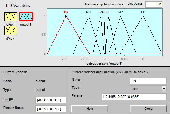
150 139

151 Appendix 3.4 Comparison Model of P&O MPPT Strategy, IncCond MPPT Strategy and FLC MPPT Strategy 140

152 141

153 Appendix 3.5 Responding Results of Comparison between P&O MPPT Strategy, IncCond MPPT Strategy and FLC MPPT Strategy in Constant Condition (.m) clc I=evalin('base','I') V=evalin('base','V') P=evalin('base','P') T=evalin('base','t') Ipv_f=evalin('base','Ipv_f') Vpv_f=evalin('base','Vpv_f') Ppv_f=evalin('base','Ppv_f') Ipv_po=evalin('base','Ipv_po') Vpv_po=evalin('base','Vpv_po') Ppv_po=evalin('base','Ppv_po') Ipv_inc=evalin('base','Ipv_inc') Vpv_inc=evalin('base','Vpv_inc') Ppv_inc=evalin('base','Ppv_inc') figure (1) plot(v,i) hold on plot(vpv_f,ipv_f,'r*') hold on plot(vpv_po,ipv_po,'bo') hold on plot(vpv_inc,ipv_inc,'k.') legend('v-i curve','fuzzy mppt','p&o mppt','inccond mppt') title('mppt V-I Curve') xlabel('voltage unit: V') ylabel('current unit: I') grid on figure (2) plot(v,p) hold on plot(vpv_f,ppv_f,'r*') hold on plot(vpv_po,ppv_po,'bo') hold on plot(vpv_inc,ppv_inc,'k.') 142

154 legend('p-v curve','fuzzy mppt','p&o mppt','inccond mppt') title('mppt V-P Curve') xlabel('voltage unit: V') ylabel('power unit: W') grid on figure (3) plot(t,ppv_f,'r-') hold on plot(t,ppv_po,'b-') hold on plot(t,ppv_inc,'k.') legend('fuzzy mppt','p&o mppt','inccond mppt') title('responding Speed of different MPPT Algorithms') xlabel('time (s)') ylabel('power (W)') grid on Appendix 3.6 Re-regulation of FIS 143

155 144

156 Appendix 3.7 The Output Curve of Comparison between P&O MPPT Strategy, IncCond MPPT Strategy and FLC MPPT Strategy in Both Temperature and Irradiation Varying Condition clc I=evalin('base','I') V=evalin('base','V') P=evalin('base','P') T=evalin('base','t') Ipv_f=evalin('base','Ipv_f') Vpv_f=evalin('base','Vpv_f') Ppv_f=evalin('base','Ppv_f') Ipv_po=evalin('base','Ipv_po') Vpv_po=evalin('base','Vpv_po') 145

157 Ppv_po=evalin('base','Ppv_po') Ipv_inc=evalin('base','Ipv_inc') Vpv_inc=evalin('base','Vpv_inc') Ppv_inc=evalin('base','Ppv_inc') figure (1) plot(v,i) hold on plot(vpv_f,ipv_f,'r.') hold on plot(vpv_po,ipv_po,'b.') hold on plot(vpv_inc,ipv_inc,'k.') legend('v-i curve','fuzzy mppt','p&o mppt','inccond mppt') title('mppt V-I Curve') xlabel('voltage unit: V') ylabel('current unit: I') grid on figure (2) plot(v,p) hold on plot(vpv_f,ppv_f,'r.') hold on plot(vpv_po,ppv_po,'b.') hold on plot(vpv_inc,ppv_inc,'k.') legend('p-v curve','fuzzy mppt','p&o mppt','inccond mppt') title('mppt V-P Curve') xlabel('voltage unit: V') ylabel('power unit: W') grid on figure (3) plot(t,ppv_f,'r-') hold on plot(t,ppv_po,'b-') hold on plot(t,ppv_inc,'k-') legend('fuzzy mppt','p&o mppt','inccond mppt') title('responding Speed of different MPPT Algorithms') xlabel('time (s)') ylabel('power (W)') 146

158 grid on Appendix 4.1 Shading Main Program: PVprog [4-2] clc % This is the main program which calls programs PVprog2 and PVprog3. Therefore % you will be required to download all these three programs. % Input should be provided in such a way that the group with lowest % insolation should be entered first and then the data should be entered % into the ascending order with respect to the insolation. i.e. the final % entry should be of the group with uniform full or maxiimum insolation. no_parallel_config=input('number of groups :'); col_plot=['b' 'g' 'r' 'c' 'm' 'y' 'k']; for j=1:no_parallel_config fprintf('\n'); fprintf('data OF GROUP NUMBER NO. %d \n',j); S{j,1}=input('Number of subassemblies in an assembly : '); S{j,2}=input('Modules in subassembly; Temp; Insolation : '); S{j,3}=input('Number of such assemblies in a group : '); end for i=1:no_parallel_config N(i)=S{i,3}(1,1); assemblies in a group Sub_assemblies(i)=S{i,1}(1,1); subassemblies end % Number of % Number of for k=1:no_parallel_config for i=1:sub_assemblies(k) n(k,i)=s{k,2}(1,i); % Number of modules in subassemblies g(k,i)=s{k,2}(3,i); % Insolation on the modules on subassemblies Temp(k,i)=S{k,2}(2,i); % Temp on the modules on subassemblies PVprog2(g(k,i),Temp(k,i),n(k,i),i,k); end 147

159 end del=0.5; for k=1:no_parallel_config j=0; cont=1; I=0; x=0; V=0.001; flg1(k)=1; while(v>0) I=I+0.001; x=x+1; for(j=1:1:sub_assemblies(k)) % No. of modules in subassembly* voltage of module volt_subassembly(j)=n(k,j)* PVprog3(I,g(k,j),Temp(k,j)); end V=sum(volt_subassembly); % Sum of the voltage of subassemblies in a series if (x>2) dev_v=vsum_last-v; if (dev_v>4) I=I ; for(j=1:1:sub_assemblies(k)) % No. of modules in subassembly* voltage of module volt_subassembly(j)=n(k,j)* PVprog3(I,g(k,j),Temp(k,j)); end V=sum(volt_subassembly); end end Vsum_last=V; volt(1,x)=v; % voltage of a group curr(1,x)=i*n(k); % total current from similar series assemblies i.e from group power(1,x)=volt(1,x)*curr(1,x); % power from group volt1(k,x)=volt(1,x); curr1(k,x)=curr(1,x); power1(k,x)=power(1,x); 148

160 end curradj(k)=curr(1,x); curr_seriesassembly(1,:)=curr(1,:)/n(k); power_seriesassembly(1,:)=power(1,:)/n(k); figure(2*no_parallel_config+1); hold on; legend('g1','g2','g3') %FOR FIXED 3 GROUPS title('i-v characteristics of series assemblies'); plot(volt(1,:),curr_seriesassembly(1,:),col_plot(k)); figure (no_parallel_config*2+2); hold on; legend('g1','g2','g3') title('p-v characteristics of series assemblies'); plot(volt(1,:),power_seriesassembly(1,:),col_plot(k)); figure (no_parallel_config*2+3); hold on; legend('g1','g2','g3') title('i-v characteristics of Groups'); plot(volt(1,:),curr(1,:),col_plot(k)) figure (no_parallel_config*2+4); hold on; legend('g1','g2','g3') title('p-v characteristics of Groups'); plot(volt(1,:),power(1,:),col_plot(k)) VIP=[volt;curr;power]; clear curr clear power; clear curr_seriesassembly; clear power_seriesassembly; len(k)=length(volt); %Store the lengths of the voltage vectors related to each curve clear volt; % Minimising the number of points on final output curves for i=1:length(vip) VIP(1,i)=round(VIP(1,i)); end for i=1:(length(vip)-1) if(vip(1,i)==vip(1,i+1)) VIP(2,i+1)=VIP(2,i); VIP(3,i+1)=VIP(3,i); end 149

161 end len_count=length(vip); for i=1:len_count; VIP(1,i)=round(VIP(1,i)); end for i=1:len_count-1 if(vip(1,i)==vip(1,i+1)) VIP(2,i+1)=VIP(2,i); VIP(3,i+1)=VIP(3,i); end end p=1; z(1,p)=vip(1,1); z(2,p)=vip(2,1); z(3,p)=vip(3,1); for i=1:len_count-1 if ((i~=1)& ((VIP(1,i))~=VIP(1,i+1))) p=1+p; z(1,p)=vip(1,i+1); z(2,p)=vip(2,i+1); z(3,p)=vip(3,i+1); end end; clear VIP; for i=1:length(z) Vs(k,i)=z(1,i); Is(k,i)=z(2,i); Ps(k,i)=z(3,i); end clear z; end for k=1:no_parallel_config toglflg=0; indx=length(vs); for i=1:length(vs) if (Vs(k,i)==0 && toglflg==0) toglflg=1; indx=i; init=vs(k,indx-1); inc=length(vs)-indx; delinc=0; end if (i>=indx && i<length(vs)) 150

162 delinc=delinc+1; Vs(k,i)=(init)*(inc-delinc+1)/(inc+1); end end end for k=1:no_parallel_config for i=1:length(vs) if (i>=1 && Is(k,i)==0 ) Is(k,i)=Is(k,i-1); Ps(k,i)=Is(k,i)*Vs(k,i); end end end for i=1:length(vs) Parray(i)=0; Varray(i)=0; Iarray(i)=0; end for i=1:length(vs) Vt(i)=Vs(no_parallel_config,i); for k=1:(no_parallel_config) Vtemp=Vs(k,:); Ptemp=Ps(k,:); Itemp=Is(k,:); Pgr(k,i)=interp1(Vtemp,Ptemp,Vt(i),'linear','extrap'); Igr(k,i)=interp1(Vtemp,Itemp,Vt(i),'linear','extrap'); if Igr(k,i)<=0 Igr(k,i)=0; Pgr(k,i)=0; end Parray(i)=Pgr(k,i)+Parray(i); Iarray(i)=Igr(k,i)+Iarray(i); end if (i>1) if (Iarray(i)<Iarray(i-1)) Iarray(i)=Iarray(i-1); end end end Varray=Vt; figure; 151

163 hold on; title('i-v characteristics of an array'); plot(varray,iarray); figure; hold on; title('p-v characteristics of an array'); plot(varray,parray); VIP=[Varray;Iarray;Parray]; save VIP; clear all; clc; return Shading sub-program: PVprog2 function temp=pvprog2(sun,t,no_of_modules,subass_no,gr_no) %PVprog2.m model for the MAX-^0 solar array returns %current, voltage and power for the given illumination and temperature % %I,V are array current and voltage %Sun=num of suns where 1 Sun =1000W/m^2 col=['b' 'g' 'r' 'c' 'm' 'y' 'k']; k= 1.38e-23; %Boltzman's constant q=1.6e-19; %charge of an electron V=1; %Initialisation of the array voltage I=0; % and array current so that one enters into while loop atleast once x=0; %initialisation while (V>0); I=I+.001; x=x+1; % enter the following constants here, and the model will be % calculated based on these for 1000 W/m^2 A=1.2; % 'diode quality' factor = 2for crystalline and <2 for amorphous Vg=1.12; % band gap voltage, 1.12eV for xtal Si, 1.75 for amorphous Si Ns=36; % number of series connected cells (diodes) T1=273+25; Voc_T1=21.06/Ns; % open ckt voltage per cell at temp T1 Isc_T1=3.8; % short ckt current per cell at temp T1 T2=273+75; Voc_T2=17.05/Ns; % open ckt voltage per cell at temp T2 152

164 Isc_T2=3.92; % short ckt current per cell at temp T2 Tak = T; %array working temp Trk = ; %reference temp %when V=0 light generated current Iph_T1= array short circuit current %constant 'a' can be determined from Iac vs T Iph_T1=Isc_T1*Sun; a=(isc_t2-isc_t1)/isc_t1*1/(t2-t1); Iph=Iph_T1*(1+a*(Tak-T1)); Vt_T1=k*T1/q; % =A*kT/q Ir_T1=Isc_T1/(exp(Voc_T1/(A*Vt_T1))-1); Ir_T2=Isc_T2/(exp(Voc_T2/(A*Vt_T1))-1); b=vg*q/(a*k); Ir=Ir_T1*(Tak/T1).^(3/A).*exp(-b.*(1./Tak-1/T1)); X2v=Ir_T1/(A*Vt_T1)*exp(Voc_T1/(A*Vt_T1)); dvdi_voc=-1.15/ns/2; %dv/di at Voc per cell from manufacturer graph Rs=-dVdI_Voc-1/X2v; %series resistance per cell Vt_T=A*1.38e-23*Tak/1.6e-19; % =A*kT/q bracket=(log((iph-i)/ir+1)); flg=(isreal(bracket)& (bracket>0)); if (flg) Vtemp=Vt_T*bracket-I*Rs; if (Vtemp>0)V=Vtemp; end else V=V-0.001; I=I ; end if (V<0) V=0; end; volt(x)=36*v*no_of_modules; curr(x)=i; power(x)=volt(x)*curr(x); end figure(2*gr_no-1); Grid on; hold on; plot(volt,curr,col(subass_no)); char GR_NO=Gr_no; 153

165 titl1 = 'IV characteristics for subassemblies of Group-'; GR_NO=num2str(Gr_no); tit = strcat(titl1,gr_no); Title(tit); Xlabel('Voltage (V)'); Ylabel('Current (A)'); figure(2*gr_no); Grid on; hold on; plot(volt,power,col(subass_no)); titl1 = 'PV characteristics for subassemblies of Group-'; tit = strcat(titl1,gr_no); Title(tit); Xlabel('Voltage (V)') Ylabel('Power (W)'); temp=[curr;volt;power]; return Shading sub-program: PVprog3 function V=PVprog3(I,Sun,T) %PVprog3.m model for the solar array %takes input as illumination, sun and temperature %V=PVprog3(G,T)returns the array voltage %I,V are array current and voltage %Sun=num of suns where 1 Sun =1000W/m^2 k= 1.38e-23; %Boltzman's constant q=1.6e-19; %charge of an electron Vc=0.01; % enter the following constants here, and the model will be % calculated based on these for 1000 W/m^2 A=1.2; % 'diode quality' factor = 2for crystalline and <2 for amorphous Vg=1.12; % band gap voltage, 1.12eV for xtal Si, 1.75 for amorphous Si Ns=36; % number of series connected cells (diodes) Voc_T1=21.06/Ns; Isc_T1=3.8; T1=273+25; % open ckt voltage per cell at temp T1 % short ckt current per cell at temp T1 154

166 Voc_T2=17.05/Ns; Isc_T2=3.92; T2=273+75; % open ckt voltage per cell at temp T2 % short ckt current per cell at temp T2 Tak =273+T; Trk =273+25; %array working temp %reference temp %when V=0 light generated current Iph_T1= array short circuit current %constant 'a' can be determined from Iac vs T Iph_T1=Isc_T1*Sun; a=(isc_t2-isc_t1)/isc_t1*1/(t2-t1); Iph=Iph_T1*(1+a*(Tak-T1)); Vt_T1=k*T1/q; % =A*kT/q Ir_T1=Isc_T1/(exp(Voc_T1/(A*Vt_T1))-1); Ir_T2=Isc_T2/(exp(Voc_T2/(A*Vt_T1))-1); b=vg*q/(a*k); Ir=Ir_T1*(Tak/T1).^(3/A).*exp(-b.*(1./Tak-1/T1)); X2v=Ir_T1/(A*Vt_T1)*exp(Voc_T1/(A*Vt_T1)); dvdi_voc=-1.15/ns/2; %dv/di at Voc per cell from manufacturer graph Rs=-dVdI_Voc-1/X2v; %series resistance per cell Vt_T=A*1.38e-23*Tak/1.6e-19; % =A*kT/q %%%%Cheaking The Condition That log((iph-i+ir)/ir) Is Real Or Not%%%%%%% po=log((iph-i+ir)/ir); if(isreal(po) & (po>0)) Vc=(Vt_T*po)-I*Rs; if (Vc>0) Vc=Vc; end else Vc=Vc-0.01; end if(vc<0) Vc=0; end 155

167 V=Vc*Ns; Appendix 4.2 Processing Time Varying Data from MATLAB M.file to SIMULINK In Time Series Tools design: 156

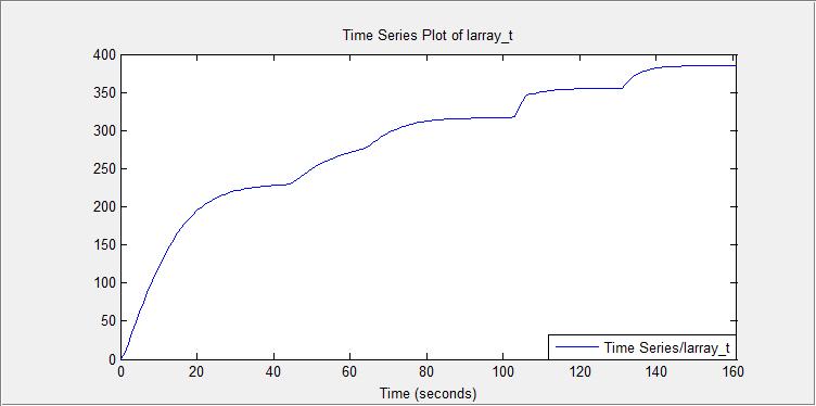
168 157

169 When importing the previous data to SIMULINK for future analysis and design, the goal could not be achieved for the version problem. Appendix 5.1Tuning Results of PID Controller 2 158

170 Appendix 5.2 System synchronous frame control with PI controller in PSCAD System modeling for constant illumination level 159