Single Image Blind Deconvolution with Higher-Order Texture Statistics

Transcription

1 Single Image Blind Deconvolution with Higher-Order Texture Statistics Manuel Martinello and Paolo Favaro Heriot-Watt University School of EPS, Edinburgh EH14 4AS, UK Abstract. We present a novel method for solving blind deconvolution, i.e., the task of recovering a sharp image given a blurry one. We focus on blurry images obtained from a coded aperture camera, where both the camera and the scene are static, and allow blur to vary across the image domain. As most methods for blind deconvolution, we solve the problem in two steps: First, we estimate the coded blur scale at each pixel; second, we deconvolve the blurry image given the estimated blur. Our approach is to use linear high-order priors for texture and second-order priors for the blur scale map, i.e., constraints involving two pixels at a time. We show that by incorporating the texture priors in a least-squares energy minimization we can transform the initial blind deconvolution task in a simpler optimization problem. One of the striking features of the simplified optimization problem is that the parameters that define the functional can be learned offline directly from natural images via singular value decomposition. We also show a geometrical interpretation of image blurring and explain our method from this viewpoint. In doing so we devise a novel technique to design optimally coded apertures. Finally, our coded blur identification results in computing convolutions, rather than deconvolutions, which are stable operations. We will demonstrate in several experiments that this additional stability allows the method to deal with large blur. We also compare our method to existing algorithms in the literature and show that we achieve state-of-the-art performance with both synthetic and real data. Keywords: coded aperture, single image, image deblurring, depth estimation. 1 Introduction Recently there has been enormous progress in image deblurring from a single image. Perhaps one of the most remarkable results is to have shown that it is possible to extend the depth of field of a camera by modifying the camera optical response [1 7]. Moreover, techniques based on applying a mask at the lens aperture have demonstrated the ability to recover a coarse depth of the This research was partly supported by SELEX Galileo grant SELEX/HWU/ 2010/SOW3.

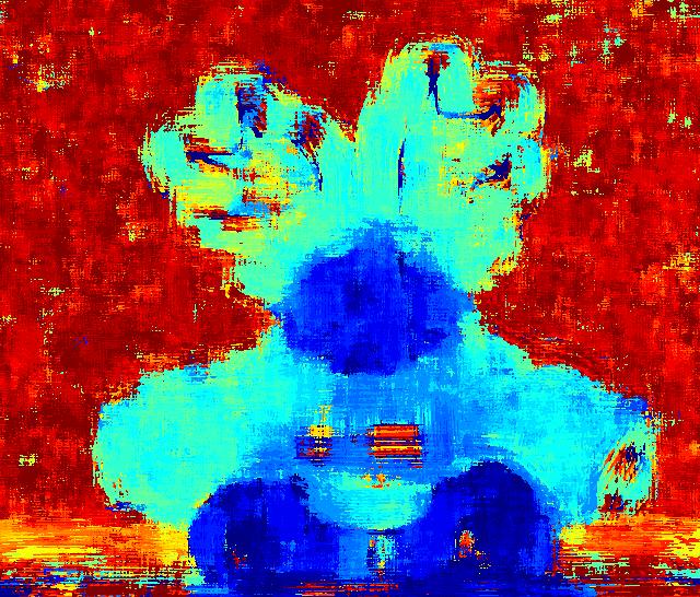
2 2 Manuel Martinello, Paolo Favaro (a) (b) Fig. 1. Results on an outdoor scene [exposure time 1/200s]. (a) Blurry coded image captured with mask b (see Fig. 4). (b) Sharp image reconstructed with our method. scene [4, 5, 8]. Depth has then been used for digital refocusing [9] and advanced image editing. In this paper we present a novel method for image deblurring and demonstrate it on blurred images obtained from a coded aperture camera. Our algorithm uses as input a single blurred image (see Fig. 1 (a)) and automatically returns the corresponding sharp one (see Fig. 1 (b)). Our main contribution is to provide a computationally efficient method that achieves state-of-the-art performance in terms of depth and image reconstruction with coded aperture cameras. We demonstrate experimentally that our algorithm can deal with larger amounts of blur than previous coded aperture methods. One of the leading approaches in the literature [5] recovers a sharp image by sequentially testing a deconvolution method for several given hypotheses for the blur scale. Then, the blur scale that yields a sharp image that is consistent with both the model and the texture priors is chosen. In contrast, in our approach we show that one can identify the blur scale by computing convolutions, rather than deconvolutions, of the blurry image with a finite set of filters. As a consequence, our method is numerically stable especially when dealing with large blur scales. In the next sections, we present all the steps needed to define our algorithm for image deblurring. The task is split in two steps: First the blur scale is identified and second, the coded image is deblurred with the estimated blur scale. We present an algorithm for blur scale identification in section 3.1. Image deblurring is then solved iteratively in section 3.2. A discussion on mask selection is then presented in section 4.1. Comparisons to existing methods are shown in section Prior Work This work relates to several fields ranging from computer vision to image and signal processing, and from optics to astronomy and computer graphics. For simplicity, we group past work based on the technique being employed.

3 Single Image Blind Deconvolution with Higher-Order Texture Statistics 3 Coded Imaging: Early work in coded imaging appears in the field of astronomy. One of the most interesting pattern designs is the Modified Uniformly Redundant Arrays (MURA) [10] for which a simple coding and decoding procedure was devised (see one such pattern in Fig. 4). In our tests the MURA pattern seems very well behaved, but too sensitive to noise (see Fig. 5). Coded patterns have also been used to design lensless systems, but these systems require either long exposures or are sensitive to noise [11]. More recently, coding of the exposure [12] or of the aperture [4] has been used to preserve high spatial frequencies in blurred images so that deblurring is well-posed. We test the mask proposed in [4] and find that it works well for image deblurring, but not for blur scale identification. A mask that we have tested and has yielded good performance is the four-holes mask of Hiura and Matsuyama [13]. In [13] however, the authors used multiple images. A study on good apertures for deblurring multiple coded images via Wiener filtering has instead led to two novel designs [14, 15]. Although the masks were designed to be used together, we have tested each of them independently for comparisons purposes. We found, as predicted by the authors, that the masks are quite robust to noise and quite well designed for image deblurring. Image deblurring and depth estimation with a coded aperture camera has also been demonstrated by Levin et al. [5]. One of their main contributions is the design of an optimal mask. We indeed find this mask quite effective both on synthetic data and real data. However, as already noticed in [16], we have found that the coded aperture technique, if approached as in [5], fails when dealing with large blur amounts. The method we propose in this paper, instead, overtakes this limitation, especially when using the four-hole mask. Finally, a design based on annular masks has also been proposed in [17] and has been exploited for depth estimation in [3]. We also tested this mask in our experiments, but, contrary to our expectations, we did not find its performance superior to the other masks. 3D Point Spread Functions: While there are several techniques to extract depth from images, we briefly mention some recent work by Greengard et al. [18] because their optical design included and exploited diffraction effects. They investigated 3D point spread functions (PSF) whose transverse cross sections rotate as a result of diffraction, and showed that such PSFs yield an order of magnitude increase in the sensitivity with respect to depth variations. The main drawback however, is that the depth range and resolution is limited due to the angular resolution of the reconstructed PSF. Depth-Invariant Blur: An alternative approach to coded imaging is wavefront coding. The key idea is to use aspheric lenses to render the lens point spread function (PSF) depth-invariant. Then, shift-invariant deblurring with a fixed known blur can be applied to sharpen the image [19, 20]. However, while the results are quite promising, the PSF is not fully depth-invariant and artifacts are still present in the reconstructed image. Other techniques based on depthinvariant PSFs exploit the chromatic aberrations of lenses [7] or use diffusion [21]. However, in the first case, as the focal sweep is across the spectrum, the method is mostly designed for grayscale imaging. While the results shown in

4 4 Manuel Martinello, Paolo Favaro these recent works are stunning, there are two inherent limitations: 1) Depth is lost in the imaging process; 2) In general, as method based on focal sweep are not exactly depth-invariant, the deblurring performance decays for objects that are too close or too far away from the camera. Multiple viewpoint: The extension of the depth of field can also be achieved by using multiple images and/or multiple viewpoints. One technique is to obtain multiple viewpoints by capturing multiple coded images [8, 13, 22] or by capturing a single image by using a plenoptic camera [9, 6, 23, 24]. These methods however, exploit multiple images or require a more costly optical design (e.g., a calibrated microlens array). Motion Deblurring and Blind Deconvolution: This work also relates to work in blind deconvolution, and in particular on motion deblurring. There has been a quite steady progress in uniform motion deblurring [25 29] thanks to the modeling and exploitation of texture statistics. Although these methods deal with an unknown and general blur pattern, they assume that blur is not changing across the image domain. More recently, the space-varying case has been studied [30 32] albeit with some restrictions on the type of motion or the scene depth structure. Blurred face recognition: Work in the recognition of blurred faces [33] is also related to our method. Their approach extracts features from motionblurred images of faces and then uses the subspace distance to identify the blur. In contrast, our method can be applied to space-varying blur and our analysis provides a novel method to evaluate (and design) masks. 2 Single Image Blind Deconvolution Blind deconvolution from a single image is a very challenging problem: We need to recover more unknowns than the available observations. This challenge will be illustrated in the next section, where we present the image formation model of a blurred image obtained from a coded aperture camera. To make the problem feasible and well-behaved, one can introduce additional constraints on the solution. In particular, we constrain the higher-order statistics of sharp texture (sec. 2.2) and impose that the blur scale be piecewise smooth across the image pixels (sec. 2.3). 2.1 Image Model In the simplest instance, a blurred image of a plane facing the camera can be described via the convolution of a sharp image with the blur kernel. However, the convolutional model breaks down with more general surfaces and, in particular, at occlusion boundaries. In this case, one can describe a blurred image with a linear model. For the sake of notational simplicity, we write images as column vectors, where all pixels are sorted in lexicographical order. Thus, a blurred image with N pixels is a column vector g R N. Similarly, a sharp image with

5 Single Image Blind Deconvolution with Higher-Order Texture Statistics 5 M pixels is a column vector f R M. Then, g satisfies g = H d f, (1) where the N M matrix H d represents the coded blur. d is a column vector with M pixels and collects the blur scale corresponding to each pixel of f. The i-th column of H d is an image, rearranged as a vector, of the coded blur with scale d i generated by the i-th pixel of f. Notice that this model is indeed a generalization of the convolutional case. In the convolutional model, H d reduces to a Toeplitz matrix. Our task is to recover the unknown sharp image f given the blurred image g. To achieve this goal it is necessary to recover the blur scale at each pixel d. The theory of linear algebra tells us that: If N = M and the equations in eq. (1) are not linearly dependent, and we are given both g and H d, then we can recover the sharp image f. However, in our case we are not given the matrix H d and the blurred image g is affected by noise. This introduces two challenges: First, to obtain H d we need to retrieve the blur scale d; second, because of noise in g and of the ill-conditioning of the linear system in eq. (1), the estimation of f might be unstable. The first challenge implies that we do not have a unique solution. The second challenge implies that even if the solution were unique, its estimation would not be reliable. However, not all is lost. It is possible to add more equations to eq. (1) until a unique reliable solution can be obtained. This technique is based on observing that, typically, one expects the unknown sharp image and blur scale map to have some regularity. For instance, both sharp textures and blur scale maps are not likely to look like noise. In the next two sections we will present and illustrate our sharp image and blur scale priors. 2.2 Sharp Image Prior Images of the real world exhibit statistical regularities that have been studied intensively in the past 20 years and have been linked to the human visual system and its evolution [34]. For the purpose of image deblurring, the most important aspect of this study is that natural images form a much smaller subset of all possible images. In general, the characterization of the statistical properties of natural images is done by applying a given transform, typically related to a component of human vision. Among the most common statistics used in image processing are the second order statistics, i.e., relations between pairs of pixels. For instance, this category includes the distributions of image gradients [35, 36]. However, a more accurate account of the image structure can be captured with high-order statistics, i.e., relations between several pixels. In this work, we consider this general case, but restrict the relations to linear ones of the form Σf 0 (2) where Σ is a rectangular matrix. Eq. (2) implies that all sharp images live approximately on a subspace. Despite their crude simplicity, these linear constraints allow for some flexibility. For example, the case of second-order statistics

6 6 Manuel Martinello, Paolo Favaro results in rows of Σ with only two nonzero values. Also, by designing Σ one can selectively apply the constraints only on some of the pixels. Another example is to choose each row of Σ as a Haar feature applied to some pixels. Notice that in our approach we do not make any of these choices. Rather, we estimate Σ directly from natural images. Natural image statistics, such as gradients, typically exhibit a peaked distribution. However, performing inference on such distributions results in minimizations of non convex functionals for which we do not have probably optimal algorithms. Furthermore, we are interested in simplifying the optimization task as much as possible to gain in computational efficiency. This has led us to enforce the linear relation above by minimizing the convex cost Σf 2 2. (3) As we do not have an analytical expression for Σ that satisfies eq. (2), we need to learn it directly from the data. We will see later that this step is necessary only when performing the deconvolution step given the estimated blur. Instead, when estimating the blur scale our method allows us to use Σ implicitly, i.e., without ever recovering it. 2.3 Blur Scale Prior The statistics of range images can be characterized with an approach similar to that for optical images [37]. The study in [37] verified the random collage model, i.e., that a scene is a collection of piecewise constant surfaces. This has been observed in the distributions of Haar filter responses on the logarithm of the range data, which showed strong cusps in the isoprobability contours. Unfortunately, a prior following these distributions faithfully would result in non convex energy minimization. A practical convex solution to enforce the piecewise constant model, is to use total variation [38]. Common choices are the isotropic and anisotropic total variation. In our algorithm we have implemented the latter. We minimize d 1, i.e., the sum of the absolute value of the components of the gradient of d. 3 Blur Scale Identification and Image Deblurring We can combine the image model introduced in sec. 2.1 with the priors in sec. 2.2 and 2.3 and formulate the following energy minimization problem: ˆd, ˆf = argmin g H d f α Σf β d 1, (4) d,f where the parameters α, β > 0 determine the amount of regularization for texture and blur scale respectively. Notice that the formulation above is common to many approaches including, in particular, [5]. Our approach, however, in addition to using a more accurate blur matrix H d, considers different priors and a different depth identification procedure.

7 Single Image Blind Deconvolution with Higher-Order Texture Statistics 7 Our next step is to notice that, given d, the proposed cost is simply a leastsquares problem in the unknown sharp texture f. Hence, it is possible to compute f in closed-form and plug it back in the cost functional. The result is a much simpler problem to solve. We summarize all the steps in the following Theorem: Theorem 1. The set of extrema of the minimization (4) coincides with the set of extrema of the minimization ˆd = argmin Hd g β d 1 ( d ) 1 (5) ˆf = ασ T Σ + H Ṱ H d ˆd H Ṱ g d where H d. = I H d ( ασ T Σ + H T d H d) 1 H T d, and I is the identity matrix. Proof. See Appendix. Notice that the new formulation requires the definition of a square and symmetric matrix Hd. This matrix depends on the parameter α and the prior matrix Σ, both of which are unknown. However, for the purpose of estimating the unknown blur scale map d, it is possible to bypass the estimation of α and Σ by learning directly the matrix Hd from data. 3.1 Learning Procedure and Blur Scale Identification We break down the complexity of solving eq. (5) by using local blur uniformity, i.e., by assuming that blur is constant within a small region of pixels. Then, we further simplify the problem by considering only a finite set of L blur sizes d 1,..., d L. In practice, we find that both assumptions work well. The local blur uniformity holds reasonably well except at occluding boundaries, which form a small subset of the image domain. At occluding boundaries the solution tends to favor small blur estimates. We also found experimentally that the discretization is not a limiting factor in our method. The number of blur sizes L can be set to a value that matches the level of accuracy of the method without reaching a prohibitive computational load. Now, by combining the assumptions we find that eq. (5) at one pixel x can be approximated by ˆd(x) = argmin Hd (x)g β d(x) 1 (6) d(x) ˆd(x) = argmin Hd(x) g x 2 2 (7) d(x) where g x is a column vector of δ 2 pixels extracted from a δ δ patch centered at the pixel x of g. Experimentally, we find that the size δ of the patch should not be smaller than the maximum scale of the coded blur in the captured image g. H d(x) is a δ2 δ 2 matrix that depends on the blur size d(x) {d 1,..., d L }.

8 8 Manuel Martinello, Paolo Favaro So we assume that Hd (x, y) 0 for y such that y x 1 > δ/2. Notice that the term β d 1 drops because of the local blur uniformity assumption. The next step is to explicitly compute Hd(x). Since the blur size d(x) is one of L values, we only need to compute Hd 1,..., Hd L matrices. As each Hd i depends on α and the local Σ, we propose to learn each Hd i directly from data. Suppose that we are given a set of T column vectors g x1,..., g xt extracted from blurry images of a plane parallel to the camera image plane. The column vectors will all share the same blur scale d i. Hence, we can rewrite the cost functional in eq. (7) for all x as Hd i G i 2 2 (8). where G i = [gx1 g xt ]. By definition of G i, Hd i G i 2 2 = 0. Hence, we find that Hd i can be computed via the singular value decomposition of G i = U i S i Vi T. If U i = [U di Q di ] where Q di corresponds to the singular values of S i that are zero (or negligible), then Hd i = Q di Q T d i. The procedure is then repeated for each blur scale d i with i = 1,..., L. Next, we can use the estimated matrices Hd 1,..., Hd L on a new image g and optimize with respect to d: ˆd = argmin Hd(x) g x β d(x) 1. (9) d x The first term represents unitary terms, i.e., terms that are defined on single pixels; the second term represents binary terms, i.e., terms that are defined on pairs of pixels. The minimization problem (9) can then be solved efficiently via graph cuts [39]. Notice that the procedure above can be applied to other surfaces as well, so that instead of a collection of parallel planes, one can consider, for example, a collection of quadratic surfaces. Also, notice that there are no restrictions on the size of a patch. In particular, the same procedure can be applied to a patch of the size of the input image. In our experiments for depth estimation, however, we consider only small patches and parallel planes as local surfaces. 3.2 Image Deblurring In the previous section we have devised a procedure to compute the blur scale at each pixel d. In this section we assume that d is given and devise a procedure to compute the image f. In principle, one could use the closed-form solution ( ) 1 f = ασ T Σ + H Ṱ H d ˆd H Ṱ g. (10) However, notice that computing this equation entails solving a large matrix inversion, which is not practical for moderate image dimensions. A simpler approach is to solve the least squares problem (4) in f via an iterative method. Therefore, we consider solving the problem ˆf = argmin g H ˆdf α Σf 2 2 (11) f d

9 Single Image Blind Deconvolution with Higher-Order Texture Statistics 9 by using a least-squares conjugate gradient descent algorithm in f [40]. The main component for the iteration in f is the gradient E f of the cost (11) with respect to f ( ) E f = ασ T Σ + H Ṱ H d ˆd f H Ṱ g. (12) d The descent algorithm iterates until E f 0. Because of the convexity of the cost functional with respect to f, the solution is also a global minimum. To compute Σ we use a database of sharp images F = [f 1 f T ] where {f i } i=1,...,t are sharp images rearranged as column vectors, and compute the singular value decomposition F = U F Σ F V T F. Then, we partition U F = [U F,1 U F,2 ] such that U F,2 corresponds to the smallest singular values of Σ F. The high-order prior is defined as Σ. = U F,2 U T F,2, such that we have Σf i 0. The regularization parameter α is instead manually tuned. The matrix H ˆd is computed as described in Section A Geometric Viewpoint on Blur Scale Identification In the previous sections we have seen that the blur scale at each pixel can be obtained by minimizing eq. (9). We search among matrices Hd 1,..., Hd L the one that yields the minimum l 2 norm when applied to the vector g x. We show that this has a geometrical interpretation: Each matrix Hd i defines a subspace and Hd i g x 2 2 is the distance of each vector g x from that subspace. Recall that Hd i = Q di Q T d i and that U i = [U di Q di ] is an orthonormal matrix. Then, we obtain that Hd i g x 2 2 = Q di Q T d i g x 2 2 = Q T d i g x 2 2 = g x 2 2 Ud T i g x 2 2. If we now divide by the scalar number g x 2 2, we obtain exactly the square of the subspace distance [41] M(g, U di ) = K ( ) 2 1 Ud T g i,j (13) g where K is the rank of the subspace U di, U di = [U di,1... U di,k], and U di,j, j = 1,, K are orthonormal vectors. The geometrical interpretation brings a fresh look to image blurring and deblurring. Consider the image model (1). Let us take the singular value decomposition of the blur matrix H d j=1 H d = U d S d V T d (14) where S d is a diagonal matrix with positive entries, and both U d and V d are orthonormal matrices. Formally, the vector f undergoes a rotation (Vd T ), then a scaling (S d ), and then again another rotation (U d ). This means that if f lives in a subspace, the initial subspace is mapped to another rotated subspace, possibly of smaller dimension (see Fig. 2, middle). Notice that as we change the blur scale, the rotations and scaling are also changing and may result in yet a different subspace (see Fig. 2, right).

10 10 Manuel Martinello, Paolo Favaro f 2 f 3 f 1 (a) H d1 g 1 g 2 g 3 (b) H d2 g 1 g 2 (c) g 3 Fig. 2. Coded images subspaces. (a) Image patches on a subspace. (b) Subspace containing images blurred with H d1 ; blurring has the effect of rotating and possibly reducing the dimensionality of the original subspace. (c) Subspace containing images blurred with H d2. It is important to understand that rotations of the vector f can result in blurring. To clarify this, consider blurred and sharp images with only 3 pixels (we cannot visualize the case of more than 3 pixels), i.e., g 1 = [g 1,x g 1,y g 1,z ] T and f 1 = [f 1,x f 1,y f 1,z ] T. Then, we can plot the vectors g 1 and f 1 as 3D points (see Fig. 2). Let g 1 = 1 and f 1 = 1. Then, we can rotate f 1 about the origin and overlap it exactly on g 1. In this case rotation corresponded to blurring. The opposite is also true. We can rotate the vector g 1 onto the vector f 1 and thus perform deblurring. Furthermore, notice that in this simple example the most blurred images are vectors with identical entries. Such blurred images lie along the diagonal direction [1 1 1] T. In general, blurry images tend to have entries with similar values and hence tend to cluster around the diagonal direction. Our ability to discriminate between different blur scales in a blurry image boils down to being able to determine the subspaces where the patches of such blurry image live. If sharp images do not live on a subspace, but uniformly in the entire space, our only way to distinguish the blur size is that the blurring H d scales some dimensions of f to zero and that the scaling varies with blur size. This case has links to the zero-sheet approach in the Fourier domain [42]. However, if the sharp images live on a subspace, the blurring H d may preserve

11 Single Image Blind Deconvolution with Higher-Order Texture Statistics 11 Input: A single coded image g and a collection of coded images of L planar scenes. Output: The blur scale map d of the scene. Preprocessing (offline) Pick an image patch size larger than twice the maximum blur scale; for i = 1,..., L do Compute the singular value decomposition U is ivi T of a collection of image patches coded with blur scale d i ; Calculate the subspace U di as the columns of U i corresponding to nonzero singular values of S i; end Blur identification (online) Solve ˆd = arg min d {d1,,d L } Px M2 (g x, U d ) + β d(x) g x Algorithm 1: Blur scale identification from a single coded image via the subspace distance method. all the directions and blur scale identification is still possible by determining the rotation of the sharp images subspace. This is the principle that we exploit. Notice that the evaluation of the subspace distance M involves the calculation of the inner product between a patch and a column of U di. Hence, this calculation can be done exactly as the convolution of a column of U di, rearranged as an image patch, with the whole image g. We can conclude that the algorithm requires computing a set of L K convolutions with the coded image, which is a stable operation of polynomial computational complexity. As we have shown that minimizing eq. (13) is equivalent to minimizing H d i g x 2 2 up to a scalar value, we summarize the blur scale identification procedure in Algorithm Coded Aperture Selection In this section we discuss how to obtain an optimal pattern for the purpose of image deblurring. As pointed out in [19] we identify two main challenges: The first one is that accurate deblurring requires accurate identification of the blur scale; the second one is that accurate deblurring requires little texture loss due to blurring. A first step towards addressing these challenges is to define a metric for blur scale identification and a metric for texture loss. Our metric for blur scale identification can be defined directly from section 4. Indeed, the ability to determine which subspace a coded image patch belongs to can be measured via the distance between the subspaces associated to each blur scale M(U d1, U d2 ) = K ( 2. Ud T U 1,i d 2,j) (15) i,j Clearly, the wider apart all the subspaces are, and the less prone to noise the subspace association is. We find that a good visual summary of the spacing

12 12 Manuel Martinello, Paolo Favaro d20 d25 d d20 d25 d d10 M( (Ud10, Ud20) =!K d10 d25 M( (Ud25, Ud25) = 0 d25 d (a) Ideal distance matrix d (b) Circular aperture Fig. 3. Distance matrix computation. The top-left corner of each matrix is the distance between subspaces corresponding to small blur scales, and, vice versa, the Tuesday, 15 February 2011 Tuesday, 15 February 2011 bottom-right corner is the distance between subspaces corresponding to large blur scales. Notice that large subspace distances are bright and small subspace distances are dark. The maximum distance ( K) is achievable when two subspaces are orthogonal to each other. between all the subspaces is a (symmetric) matrix with distances between any two subspaces. We compute such matrix for a conventional camera and show the results in Fig. 3, together with the ideal distance matrix. In each distance matrix, subspaces associated to blur scales ranging from the smallest to the largest ones are arranged along the rows from left to right and along the columns from top to bottom. Along the diagonal the distance is necessarily 0 as we compare identical subspaces. Also, by definition the metric cannot exceed K, where K is the minimum rank among the subspaces. In Fig. 5 we report the distance matrices computed for each of the apertures we consider in this work (see Fig. 4). Notice that the subspace distance map for a conventional camera (Fig. 3(b)) is overall darker than the matrices for coded aperture cameras (Fig. 5). This shows the poor blur scale identifiability of the circular aperture and the improvement that can be achieved when using a more elaborate pattern. The rank K can be used to address the second challenge, i.e., the definition of a metric for texture loss. So far we have seen that blurring can be interpreted as a combination of rotations and scaling. Deblurring can then be interpreted as a combination of rotations and scaling in the opposite direction. However, when blurring scales some directions to 0, part of the texture content has been lost. This suggests that a simple measure for texture loss is the dimension of the coded subspace: The higher the dimension and the more texture content we can restore. As the (coded images) subspace dimension is K, we can immediately conclude that the subspace distance matrix that most closely resembles the ideal distance matrix (see Fig. 3(a)) is the one that simultaneously achieves the best depth identification and the least texture loss. Finally, we propose to use the average L 1 fitting of any distance matrix to the ideal distance matrix scaled of K, i.e., K(11 T I) M. The fitting yields the values in Table 1. We can

13 Single Image Blind Deconvolution with Higher-Order Texture Statistics 13 (a) (b) (c) (d) (e) (f) (g) (h) Fig. 4. Coded aperture patterns and PSFs. All the aperture patterns we consider in this work (top row) and their calibrated PSFs for two different blur scales (second and bottom row). (a) and (b) aperture masks used in both [13] and [43]; (c) annular mask used in [17]; (d) pattern proposed by [5]; (e) pattern proposed by [4]; (f) and (g) aperture masks used in [15]; (h) MURA pattern used in [10]. (a) Mask 4(a) (b) Mask 4(b) (c) Mask 4(c) (d) Mask 4(d) (e) Mask 4(e) (f) Mask 4(f) (g) Mask 4(g) (h) Mask 4(h) Fig. 5. Subspace distances for the eight masks in Fig. 4. Notice that the subspace rank K determines the maximum distance achievable, and therefore, coded apertures with overall darker subspace distance maps have poor blur scale identifiability (i.e., sensitive to noise). Masks 4(a) 4(b) 4(c) 4(d) 4(e) 4(f) 4(g) 4(h) L 1 fitting Table 1. L 1 fitting of any distance matrix to the ideal distance matrix scaled of K.

14 14 Manuel Martinello, Paolo Favaro also see visually in Fig. 5 that mask 4(b) and mask 4(d) are the coded apertures that we can expect to achieve the best results in texture deblurring. The quest for the optimal mask is, however, still an open problem. Even if we look for the optimal mask via brute-force search, a single aperture pattern requires the evaluation of eq. (15) and the computation of all the subspaces associated to each blur scale. In particular, the latter process requires about 15 minutes on a QuadCore 2.8GHz with Matlab 7, which makes the evaluation of a large number of masks unfeasible. Devising a fast procedure to determine the optimal mask will be subject of future work. 5 Experiments In this section we demonstrate the effectiveness of our approach on both synthetic and real data. We show that the proposed algorithm performs better than previous methods on different coded apertures and different datasets. We also show that the masks proposed in the literature do not always yield the best performance. 5.1 Performance Comparison Before proceeding with tests on real images, we perform extensive simulations to compare accuracy and robustness of our algorithm with 4 competing methods including the current state-of-the-art approach. The methods are all based on the hypothesis plane deconvolution used by [5] as explained in the Introduction. The main difference among the competing methods is that the deconvolution step is performed either using the Lucy-Richardson method [44], or regularized filtering (i.e., with image gradient smoothness), or Wiener filtering [45], or Levin s procedure [5]. We use the 8 masks shown in Fig. 4. All the patterns have been proposed and used by other researchers [4, 5, 10, 13, 15, 17]. For each mask and a given blur scale map d, we simulate a coded image by using eq. (1), where f is an image of 4, pixels with either random texture or a set of patches from natural images (examples of these patches are shown in Fig. 6). Then, for each algorithm we obtain a blur scale map estimate ˆd and compute its discrepancy with the ground-truth. The ground-truth blur scale map d that we use is shown in pseudo-colors at the top-left of both Fig. 7 and Fig. 8 and it represents a stair composed of 39 steps at different distances (and thus different blur scales) from the camera. We assume that the focal plane is set to be between the camera and the first object of interest in the scene. With this setting, the bottom part of the blur scale map (small blur sizes) corresponds to points close to the camera, and the top part (large blur sizes) to points far from the camera. Each step of the stair is a square of pixels, we have squeezed the actual illustration along the vertical axis to fit in the paper. The size of the blur ranges from 7 to 30 pixels. Notice that in measuring the errors we consider all pixels, including those at the blur scale discontinuities, given by the difference of blur scale between neighboring steps. In Fig. 7 we show, for each mask in Fig. 4,

15 Single Image Blind Deconvolution with Higher-Order Texture Statistics 15 image noise level σ= 0 image noise level σ= Fig. 6. Real texture. Some of the patches extracted from real images that have been used in our tests. The same patches are shown with no noise (top part) and when a Gaussian noise is added to them (bottom part). the results of the proposed method (right) together with the results obtained by the current state-of-the-art algorithm (left) on random texture. The same procedure, but with texture from natural images, is reported in Fig. 8. For the three best performing masks (mask 4(a), mask 4(b), and mask 4(d)), we report the results with the same graphical layout in Fig. 9, in order to better appreciate the improvement of our method over previous ones, especially for large blur scales. Every plot shows, for each of the 39 steps we consider, the mean and 3 times the standard deviation of the estimated blur scale values (ordinate axis) against the true blur scale level (abscissa axis). The ideal estimate is the diagonal line where each estimated level corresponds to the correct true blur scale level. If there is no bias in the estimation of the blur scale map, the ideal estimate should lie between 3 times the standard deviation about the mean with probability close to 1. Our method performs consistently well with all the masks and at different blur scale levels. In particular, the best performances are observed for mask 4b (Fig. 9(b)) and d (Fig. 9(c)), while the performance of competing methods rapidly degenerates with increasing pattern scales. This demonstrates that our method has potential for restoring objects at a wider range of blur scales and with higher accuracy than in previous algorithms. A quantitative comparison among all the methods and masks is given in Table 2 and Table 4 (for random texture) and in Table 3 and Table 5 (for real texture). In each table, the left half reports the average error of the blur scale estimate (measured as d ˆd 1, where d and ˆd are the ground-truth and the estimated blur scale map respectively); the right half reports the error on the reconstructed sharp image ˆf, measured as f ˆf f ˆf 2 2, where f is the ground-truth image. The gradient term is added to improve sensitivity to artifacts in the reconstruction. As one can see from Tables 2-5, several levels of noise have been considered in the performance comparison: σ = 0 (Table 2 and

16 16 Manuel Martinello, Paolo Favaro Far Close GT (a) Mask 4(a) (b) Mask 4(b) (c) Mask 4(c) (d) Mask 4(d) (e) Mask 4(e) (f) Mask 4(f ) (g) Mask 4(g) (h) Mask 4(h) Tuesday, 15 February 2011 Fig. 7. Blur scale estimation - random texture. GT: Ground-truth blur scale map. (a-h) Estimated blur scale maps for all the eight masks we consider in the paper. For each mask, the figure reports the blur scale map estimated with both Levin et al. s method (left) and our method (right). Table 3), σ = 0.001, σ = 0.002, and σ = (Table 4 and Table 5). The noise level is however adjusted to accommodate the difference in overall incoming light between the masks, i.e., if the mask i has an incoming light of li 1, the noise level for that mask is given by: 1 σi = σ. (16) li Thus, masks such as 4(f), 4(g) and 4(h) are subject to lower noise levels than masks such as 4(a) and 4(b). Our method produces more consistent and accurate blur scale maps than previous methods for both random texture and natural images, and across the 8 masks that it has been tested with. 5.2 Results on Real Data We now apply the proposed blur scale estimation algorithm to coded aperture images captured by inserting the selected mask into a Canon 50mm f /1.4 lens 1 The value of li represents the quantity of lens aperture that is open: when the lens aperture is totally open, li = 1; instead, when the mask completely blocks the light, li = 0.

17 Single Image Blind Deconvolution with Higher-Order Texture Statistics 17 Far Close GT (a) Mask 4(a) (b) Mask 4(b) (c) Mask 4(c) (d) Mask 4(d) Tuesday, 15 February 2011 (e) Mask 4(e) (f) Mask 4(f) (g) Mask 4(g) (h) Mask 4(h) Fig. 8. Blur scale estimation - real texture. GT: Ground-truth blur scale map. (a-h) Estimated blur scale maps for all the eight masks we consider in the paper. For each mask, the figure reports the blur scale map estimated with both Levin et al. s method (left) and our method (right). mounted on a Canon EOS-5D DSLR as described in [5, 15]. Based on the analysis in section 4.1 we choose mask 4(b) and mask 4(b). Each of the 4 holes in the first mask is 3.5mm large, which corresponds to the same overall section of a conventional (circular) aperture with diameter 7.9mm (f/6.3 in a 50mm lens). All indoor images have been captured by setting the shutter speed to 30ms (ISO ) while outdoors the exposure has been set to 2ms or lower (ISO 100). Firstly, we need to collect (or synthesize) a sequence of L coded images, where L is the number of blur scale levels we want to distinguish. There are two techniques to acquire these coded images: (1) If the aim is just to estimate the depth map (or blur scale map), one can capture real coded images of a planar surface with sharp natural texture (e.g., a newspaper) at different blur scale levels. (2) If the goal is to reconstruct both depth map and all-in-focus image, one has to capture the PSF of the camera at each depth level, by projecting a grid of bright dots on a plane and using a long exposure; then, coded images are simulated by applying the measured PSFs on sharp natural images collected from the web. In the experiments presented in this paper, we use the latter approach since we estimate both the blur scale map and the all-in-focus image. The PSFs have been captured on a plane at 40 different depths between 60cm and 140cm from the camera. The focal plane of the camera was set at 150cm.

18 18 Manuel Martinello, Paolo Favaro Lucy Richardson Levin Our method Lucy Richardson Levin Our method Lucy Richardson Levin Our method Estimated blur scale Estimated blur scale Estimated blur scale True blur scale True blur scale True blur scale Lucy Richardson Levin Our method Lucy Richardson Levin Our method Lucy Richardson Levin Our method Estimated blur scale Estimated blur scale Estimated blur scale True blur scale (a) Mask 4(a) True blur scale (b) Mask 4(b) True blur scale (c) Mask 4(d) Fig. 9. Comparison of the estimated blur scale levels obtained from the 3 best methods using both random (top) and real (bottom) texture. Each graph reports the performance of the algorithms with (a) masks 4(a), (b) masks 4(b), and (c) mask 4(d). Both mean and standard deviation (in the graphs, we show three times the computed standard deviation) of the estimated blur scale are shown in an errorbar with the algorithms performances (solid lines) over the ideal characteristic curve (diagonal dashed line) for 39 blur sizes. Notice how the performance dramatically changes based on the nature of texture (top row vs bottom row). Moreover, in the case of real images the standard deviation of the estimates obtained with our method are more uniform for mask 4(b) than for mask 4(d). In the case of mask 4(d) the performance is reasonably accurate only with small blur scales. In the first experiments, we show the advantage of our approach over Levin et al. s method on a scene with blur sizes similar to the ones used in the performance test. The same dataset has been captured by using mask 4(b) (see Fig. 11) and mask 4(d) (see Fig. 12). The size of the blur, especially at the background, is very large; This can be appreciated in Fig. 10(a), which shows the same scenario captured with the same camera setting, but without mask on the lens. For a fair comparison, we do not use any regularization or user intervention to the estimated blur scale maps. As already seen in the Section 5.1 (especially in Fig. 9), Levin et al. s method yields an accurate blur scale estimate with mask 4(d) when the size of the blur is small, but it fails with large amounts of blur. The proposed approach overcomes this limitation and yields to a deblurred image that in both cases, Fig. 11(e) and Fig. 12(e), is closer to the ground-truth (Fig. 10(b)). Notice also that our method gives an accurate reconstruction of the blur scale, even without using regularization (β = 0 in eq. (9)). Some artefacts are still present in the reconstructed all-in-focus images. These are mainly due to the very large size of the

19 Single Image Blind Deconvolution with Higher-Order Texture Statistics 19 Masks - (image noise level σ = 0) Methods Blur scale estimation Image deblurring a b c d e f g h a b c d e f g h Lucy-Richardson Regularized filtering Wiener filtering Levin et al.[5] Our method Table 2. Random texture. Performance (mean error) of 5 algorithms in blur scale estimation and image deblurring for the apertures in Fig. 4, assuming there is not noise. Masks - (image noise level σ = 0) Methods Blur scale estimation Image deblurring a b c d e f g h a b c d e f g h Lucy-Richardson Regularized filtering Wiener filtering Levin et al.[5] Our method Table 3. Real texture. Performance (mean error) of 5 algorithms in blur scale estimation and image deblurring for the apertures in Fig. 4, assuming there is not noise. blur and to the raw blur-scale map: When adding regularization to the blur-scale map (β > 0), the deblurring algorithm yields to better results, as one can see in the next examples. In Fig. 13 we have the same indoor scenario, but now the items are slightly closer to the focal plane of the camera; then the maximum amount of blur is reduced. Although the background is still very blur in the coded image (Fig. 13(a)), our accurate blur-scale estimation yields to a deblurred image (Fig. 13(b)), where the text of the magazine becomes readable. Since the reconstructed blur-scale map corresponds to the depth map (relative depth) of the scene, we can use it together with the all-in-focus image to generate a 3D image 2. This image, when watched with red-cyan glasses, allows one to perceive the depth information extracted with our approach. All the regularized blur-scale maps in this work are estimated from eq. (9) by setting β = 0.5; the raw maps, instead, are obtained without regularization term (β = 0). We have tested our approach on different outdoor scenes: Fig. 15 and Fig. 14. In these scenarios we apply the subspaces we have learned within 150cm from the camera to a very large range of depths. Several challenges are present in these scenes, such as occlusions, shadows, and lack of texture. Our method demonstrates robustness to all of them. Notice again that the raw blur-scale maps shown in Fig. 15(c) and Fig. 14(c) are already very close to the maps that include regularization (Fig. 15(d) and Fig. 14(d) respectively). For each dataset, a 2 In this work, a 3D image corresponds to an image captured with a stereo camera, where one lens has a red filter and the second lens has a cyan filter. When one watches this type of images with red-cyan glasses, each eye will see only one view: The shift between the two views gives the perception of depth.

20 20 Manuel Martinello, Paolo Favaro Masks - (image noise level σ = 0.001) Methods Blur scale estimation Image deblurring a b c d e f g h a b c d e f g h Lucy-Richardson Regularized filtering Wiener filtering Levin et al Our method Methods Masks - (image noise level σ = 0.002) Blur scale estimation Image deblurring a b c d e f g h a b c d e f g h Lucy-Richardson Regularized filtering Wiener filtering Levin et al Our method Methods Masks - (image noise level σ = 0.005) Blur scale estimation Image deblurring a b c d e f g h a b c d e f g h Lucy-Richardson Regularized filtering Wiener filtering Levin et al Our method Table 4. Random texture. Performance (mean error) of 5 algorithms in blur scale estimation and image deblurring for the apertures in Fig. 4, under different levels of noise. Methods Masks - (image noise level σ = 0.001) Blur scale estimation Image deblurring a b c d e f g h a b c d e f g h Lucy-Richardson Regularized filtering Wiener filtering Levin et al.[5] Our method Methods Masks - (image noise level σ = 0.002) Blur scale estimation Image deblurring a b c d e f g h a b c d e f g h Lucy-Richardson Regularized filtering Wiener filtering Levin et al Our method Methods Masks - (image noise level σ = 0.005) Blur scale estimation Image deblurring a b c d e f g h a b c d e f g h Lucy-Richardson Regularized filtering Wiener filtering Levin et al Our method Table 5. Real texture. Performance (mean error) of 5 algorithms in blur scale estimation and image deblurring for the apertures in Fig. 4, under different levels of noise.

21 Single Image Blind Deconvolution with Higher-Order Texture Statistics 21 (a) Conventional aperture (b) Ground-truth (pinhole camera) Fig. 10. (a) Picture taken with the conventional camera without placing the mask on the lens. (b)image captured by simulating a pinhole camera (f/22.0), which can be used as ground-truth for the image texture. 3D image (Fig. 14(e) and Fig. 15(e)) has been generated by using just the output of our method: the deblurred images (b) and the blur-scale maps (d). The ground-truth images have been taken by simulating a pinhole camera (f/22.0). 5.3 Computational Cost We downsample 4 times the input images from an original resolution of 12,8 megapixel (4, 368 2, 912) and use sub-pixel accuracy, in order to keep the algorithm efficient. We have seen from experiments on real data that the raw blur-scale map is already very close to the regularized map. This means that we can obtain a reasonable blur scale map very efficiently: When β = 0 the value of the blur scale at one pixel is independent of the other pixels and the calculations can be carried out in parallel. Since the algorithm takes about 5ms for processing 40 blur scale levels at each pixel, it is suitable for real-time applications. We have run the algorithm on a QuadCore 2.8GHz with 16GB memory. The code has been written mainly in Matlab 7. The deblurring procedure, instead, takes about 100s to process the whole image for 40 blur scale levels. 6 Conclusions We have presented a novel method to recover the all-in-focus image from a single blurred image captured with a coded aperture camera. The method is split in two steps: A subspace-based blur scale identification approach and an image deblurring algorithm based on conjugate gradient descent. The method is simple, general, and computationally efficient. We have compared our method to existing algorithms in the literature and showed that we achieve state of the art

22 22 Manuel Martinello, Paolo Favaro (a) Input image (b) Raw blur-scale map (c) Deblurred image (d) Raw blur-scale map (e) Deblurred image Fig. 11. Comparison on real data - mask 4(b). (a) Input image captured by using mask 4(b). (b-c) Blur-scale map and all-in-focus image reconstructed with Levins et al. s method [5]; (d-e) Results obtained from our method. (a) Input image (b) Raw blur-scale map (c) Deblurred image (d) Raw blur-scale map (e) Deblurred image Fig. 12. Comparison on real data - mask 4(d). (a) Input image captured by using mask 4(d). (b-c) Blur-scale map and all-in-focus image reconstructed with Levins et al. s method [5]; (d-e) Results obtained from our method.

23 Single Image Blind Deconvolution with Higher-Order Texture Statistics 23 (a) Input (b) All-in-focus image (c) Blur-scale map (d) 3D image Fig. 13. Close-range indoor scene [exposure time: 1/30s]. (a) coded image captured with mask 4(b); (b) estimated all-in-focus image; (c) estimated blur-scale map; (d) 3D image (to be watched with red-cyan glasses). performance in blur scale identification and image deblurring with both synthetic and real data while retaining polynomial time complexity. Appendix Proof of Theorem 1 To prove the theorem we rewrite the least squares problem in f as H d f g α Σf 2 2 = [ Hd ασ ] f [ ] g 2 = 0 H d f ḡ 2 2 (17) 2

24 24 Manuel Martinello, Paolo Favaro (a) Input image (b) Deblurred image (c) Raw blur-size map (d) Estimated blur-size map (e) 3D image (f) Ground-truth image Fig. 14. Long-range outdoor scene [exposure time: 1/200s]. (a) coded image captured with mask 4(b); (b) estimated all-in-focus image; (c) raw blur-scale map (without regularization); (d) regularized blur-scale map; (e) 3D image (to be watched with red-cyan glasses); (f) ground-truth image.

25 Single Image Blind Deconvolution with Higher-Order Texture Statistics 25 (a) Input image (b) Deblurred image (c) Raw blur-size map (d) Estimated blur-size map (e) 3D image (f) Ground-truth image Fig. 15. Mid-range outdoor scene [exposure time: 1/200s]. (a) coded image captured with mask 4(b); (b) estimated all-in-focus image; (c) raw blur-scale map (without regularization); (d) regularized blur-scale map; (e) 3D image (to be watched with red-cyan glasses); (f) ground-truth image.